ii

© Copyright by John Thomas Herbon 2004

All Rights Reserved

iii

Abstract

The reaction of methyl radicals (CH3) with molecular oxygen (O2), a rate-

controlling process in the ignition of natural gas under radical-poor conditions, has been

investigated in high-temperature shock tube experiments. The overall rate coefficient, k1

= k1a + k1b, and individual rate coefficients for the two high-temperature product

channels, (1a) producing CH3O+O and (1b) producing CH2O+OH, were determined

using ultra-lean mixtures of CH3I and O2 in Ar/He. Narrow-linewidth UV laser

absorption at 306.7 nm was used to measure OH concentrations, for which the

normalized rise time is sensitive to the overall rate coefficient k1 but relatively insensitive

to the branching ratio of the individual channels and to secondary reactions. Atomic

resonance absorption spectroscopy measurements of O-atoms were used for a direct

measurement of channel (1a). Through the combination of measurements using the two

different diagnostics, rate coefficient expressions for both channels were determined.

Over the temperature range 1590 to 2430K, k1a = 6.08x107T1.54exp(-14005/T) cm3mol-1s-1

and k1b = 68.6 T2.86exp(-4916/T) cm3mol-1s-1. The overall rate coefficient is in close

agreement with a recent ab initio calculation and one other shock tube study, while

comparison of k1a and k1b to these and other experimental studies yields mixed results. In

contrast to one recent experimental study, reaction (1b) is found to be the dominant

channel over the entire experimental temperature range.

The standard heat of formation of the hydroxyl radical (OH) at 298 K,

∆fH°298(OH), a fundamental thermochemical parameter influencing the equilibrium

constants of many combustion and atmospheric chemical reactions, has been determined

from shock tube measurements spanning the temperature range 1964 to 2718 K and at

pressures of 1 to 2.4 atm. Low-concentration, lean and stoichiometric mixtures of H2 and

O2 in Ar produce well-controlled levels of OH in a “partial equilibrium” state, with little

or no sensitivity to the reaction kinetics. The partial equilibrium OH concentrations are

iv

dependent only on the thermochemical parameters of the reacting species, with the heat

of formation of OH being the most significant and uncertain parameter. Narrow-

linewidth UV laser absorption at 306.7nm is used to measure OH concentrations with

sufficient accuracy (2-4%) to clearly determine the value of the heat of formation. Over

the entire range of experimental conditions, the average determination is ∆fH°298(OH) =

8.92 ± 0.16 kcal/mol (37.3 ± 0.67 kJ/mol) with a standard deviation of σ = 0.04 kcal/mol

(0.17 kJ/mol). This value is 0.40 to 0.48 kcal/mol (1.7 to 2.0 kJ/mol) below the

previously accepted values, and agrees with recent theoretical calculations, experimental

studies using the positive-ion cycle, and calculations using thermochemical cycles.

v

Acknowledgements

This work would not have been successful without the people and organizations

that have made my time at Stanford both possible and enjoyable.

It has been an honor to work with Prof. Ronald Hanson, who has energetically

instructed and motivated me in the methodologies for performing careful and precise

research. I am grateful to him for his willingness to take me on as a student, and his

efforts to mentor me throughout my program. I have had the unique opportunity to be

co-advised by two other very talented people, Prof. Tom Bowman and Prof. David

Golden. I have learned a tremendous amount from all three of these advisors, and it has

been a privilege to work for them.

My studies have been enhanced by my fellow graduate students who served to

both guide and encourage me. The invaluable relationships I have fostered at Stanford

are too many to enumerate. I am particularly thankful for the graduate and post-doctoral

students who were senior to me, as they provided not only stimulation and

encouragement but also instruction on numerous topics. They constantly inspired me

with their understanding of challenging research subject matter and their general know-it-

all-ness of every other conceivable random topic.

I am grateful to Ron Bates who took me under his wing as a new student and gave

me a foothold in shock tube chemical kinetics research. I am also indebted to Matthew

Oehlschlaeger, who built a new shock tube facility and then allowed me to utilize it to

finish my research. It has been a great pleasure to work along side him for the past four

years.

As the leader of the shock tube group, Dr. David Davidson has been a tremendous

man to work with, and I could not have asked for a more talented and generous person to

provide leadership for our group. His willingness to teach and advise are wonderful

assets, and I will be ever thankful for the opportunity to do research with him.

vi

I have been blessed with an incredibly supportive and loving family, who have

given me unwavering encouragement during this period of life. I have also been blessed

by our “California family” – they will make graduation and moving on a bittersweet

experience.

Most importantly, I am indebted to my loving and lovely wife, Robin, for

sacrificing so much and supporting me tirelessly for so many years. She, along with our

son, Caleb, bring ceaseless joy and contentment to my life.

This research was sponsored by the Chemical Sciences Division, Office of Basic

Energy Sciences, U.S. Department of Energy.

vii

Contents

Abstract .............................................................................................................................iii

Acknowledgements............................................................................................................ v

Contents............................................................................................................................vii

List of Tables.....................................................................................................................xi

List of Figures .................................................................................................................xiii

Chapter 1: Introduction ............................................................................................... 1

1.1 Motivation........................................................................................................ 1

1.2 Background ...................................................................................................... 2

1.2.1 CH3+O2→products.............................................................................. 2

1.2.2 The heat of formation of OH............................................................... 4

1.3 Scope and organization of thesis...................................................................... 6

Chapter 2: Experimental apparatus and diagnostics.............................................. 13

2.1 Experimental facilities ................................................................................... 13

2.1.1 Shock tube ......................................................................................... 13

2.1.2 Gas mixing facility ............................................................................ 15

2.1.3 Mixture preparation........................................................................... 16

2.2 OH laser absorption diagnostic ...................................................................... 18

2.2.1 Experimental setup............................................................................ 18

2.2.2 OH diagnostic improvements............................................................ 21

2.3 O-atom ARAS diagnostic .............................................................................. 22

2.3.1 Experimental setup............................................................................ 23

2.3.2 Calibration......................................................................................... 24

2.3.3 Absorption by other species .............................................................. 25

Chapter 3: CH3 + O2 → products.............................................................................. 29

3.1 Introduction.................................................................................................... 29

viii

3.2 Experimental apparatus.................................................................................. 30

3.3 Experimental details....................................................................................... 30

3.3.1 OH laser absorption measurements to determine k1 ......................... 30

3.3.2 O-atom ARAS measurements to determine k1a ................................ 32

3.3.3 Impurity issues .................................................................................. 33

3.3.4 Experiments....................................................................................... 36

3.4 Data and results .............................................................................................. 37

3.4.1 Experimental data.............................................................................. 37

3.4.2 Rate coefficient expressions and fit to the data................................. 38

3.5 Discussion ...................................................................................................... 39

3.5.1 Comparison to other studies.............................................................. 39

3.5.2 Constrained vs. unconstrained rate expression fits ........................... 41

3.5.3 Uncertainty analysis .......................................................................... 42

3.5.4 Secondary chemistry and OH peak sensitivity.................................. 45

3.6 Conclusions.................................................................................................... 47

Chapter 4: The heat of formation of OH.................................................................. 59

4.1 Introduction.................................................................................................... 59

4.2 Experimental apparatus.................................................................................. 59

4.3 Review of OH spectral absorption coefficients ............................................. 60

4.4 Experimental conditions ................................................................................ 61

4.5 Data and results .............................................................................................. 62

4.5.1 Experiments....................................................................................... 62

4.5.2 Fitting the data................................................................................... 63

4.5.3 Uncertainty analysis .......................................................................... 63

4.5.4 Results ............................................................................................... 64

4.6 Discussion ...................................................................................................... 66

4.6.1 Verification of the sensible enthalpy................................................. 66

4.6.2 The OH absorption oscillator strength .............................................. 66

4.6.3 Comparison to previous work ........................................................... 67

4.6.4 Implications....................................................................................... 68

4.7 Conclusions.................................................................................................... 68

ix

Chapter 5: Conclusions .............................................................................................. 75

5.1 Summary of results ........................................................................................ 75

5.1.1 CH3 + O2 → products........................................................................ 75

5.1.2 Heat of formation of OH ................................................................... 76

5.1.3 Publications ....................................................................................... 77

5.2 Recommendations for future work: Facilities and diagnostics ..................... 77

5.2.1 Facilities improvement and impurity reduction ................................ 77

5.2.2 Diagnostics improvements ................................................................ 80

5.3 Recommendations for future work: Kinetics ................................................ 84

Appendix A: Calculation of OH spectral absorption coefficients ......................... 87

A.1 Introduction.................................................................................................... 87

A.2 Spectroscopic data.......................................................................................... 88

A.3 Partition functions .......................................................................................... 90

A.4 Conclusions.................................................................................................... 95

Appendix B: Measurements of collision shift in the OH A-X(0,0) band............... 97

B.1 Introduction.................................................................................................... 97

B.1.1 Motivation ......................................................................................... 97

B.1.2 Background ....................................................................................... 98

B.2 Experimental details....................................................................................... 99

B.3 Data Reduction............................................................................................. 102

B.3.1 Preparation of the signal traces ....................................................... 102

B.3.2 Lineshape fits and collision shift measurement .............................. 105

B.3.3 Uncertainty calculations.................................................................. 106

B.4 Results and discussion ................................................................................. 107

B.4.1 Temperature dependence of collision shift ..................................... 107

B.4.2 Collision-partner dependence of collision shift .............................. 109

B.4.3 Rotational quantum number dependence of collision shift ............. 110

B.4.4 Collision-broadening measurements ............................................... 110

B.4.5 Motional narrowing and Galatry lineshapes ................................... 112

B.5 Conclusions.................................................................................................. 113

Appendix C: Shock velocity and T5, P5 uncertainty analysis............................... 129

x

C.1 Motivation.................................................................................................... 129

C.2 Shock velocity measurement and uncertainty calculation ........................... 130

C.3 Calculation of uncertainties in T5, P5 ........................................................... 133

C.4 Discussion .................................................................................................... 134

Appendix D: ARAS system design, optimization and theory .............................. 137

D.1 Atomic resonance absorption spectroscopy................................................. 137

D.2 Design and optimization considerations ...................................................... 140

D.2.1 ARAS diagnostics: monochromator vs. atomic filter .................... 140

D.2.2 Optimization of the lamp design and optics.................................... 143

D.3 Calibration and the two-layer model for the lamp ....................................... 147

Appendix E: The partial equilibrium of H2/O2 mixtures ..................................... 155

E.1 The partial equilibrium hypothesis .............................................................. 155

E.2 Solution and testing of the partial equilibrium hypothesis .......................... 157

References ...................................................................................................................... 161

xi

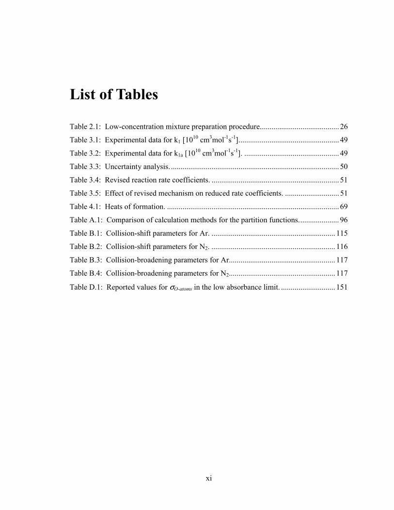
List of Tables

Table 2.1: Low-concentration mixture preparation procedure......................................... 26

Table 3.1: Experimental data for k1 [1010 cm3mol-1s-1].................................................... 49

Table 3.2: Experimental data for k1a [1010 cm3mol-1s-1]. ................................................. 49

Table 3.3: Uncertainty analysis. ....................................................................................... 50

Table 3.4: Revised reaction rate coefficients. .................................................................. 51

Table 3.5: Effect of revised mechanism on reduced rate coefficients. ............................ 51

Table 4.1: Heats of formation. ......................................................................................... 69

Table A.1: Comparison of calculation methods for the partition functions..................... 96

Table B.1: Collision-shift parameters for Ar. ................................................................ 115

Table B.2: Collision-shift parameters for N2. ................................................................ 116

Table B.3: Collision-broadening parameters for Ar....................................................... 117

Table B.4: Collision-broadening parameters for N2....................................................... 117

Table D.1: Reported values for σO-atoms in the low absorbance limit. ............................ 151

xiii

List of Figures

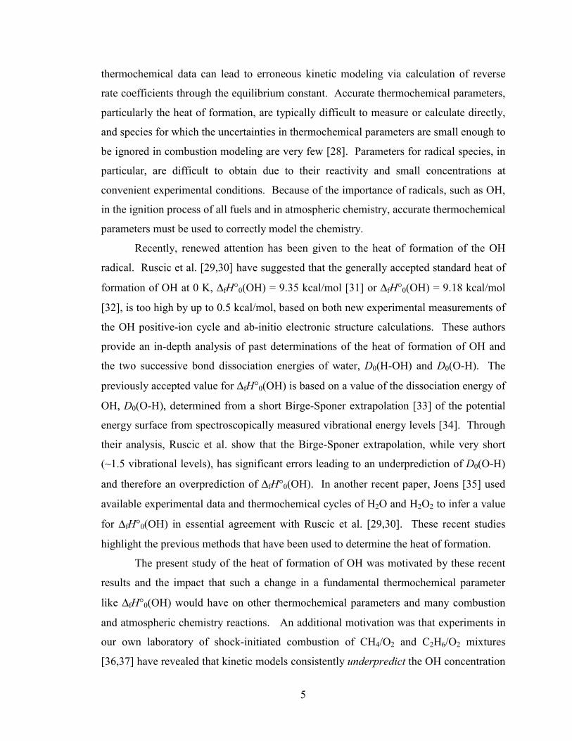
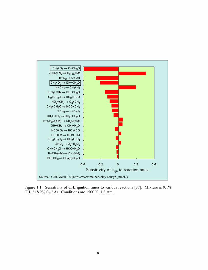
Figure 1.1: Sensitivity of CH4 ignition times to various reactions [37]. Mixture is

9.1% CH4 / 18.2% O2 / Ar. Conditions are 1500 K, 1.8 atm. ......................... 8

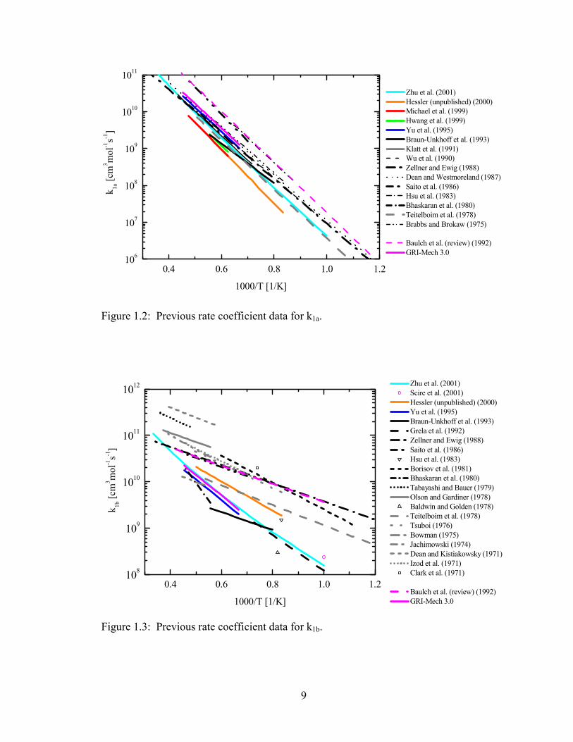
Figure 1.2: Previous rate coefficient data for k1a. .............................................................. 9

Figure 1.3: Previous rate coefficient data for k1b. .............................................................. 9

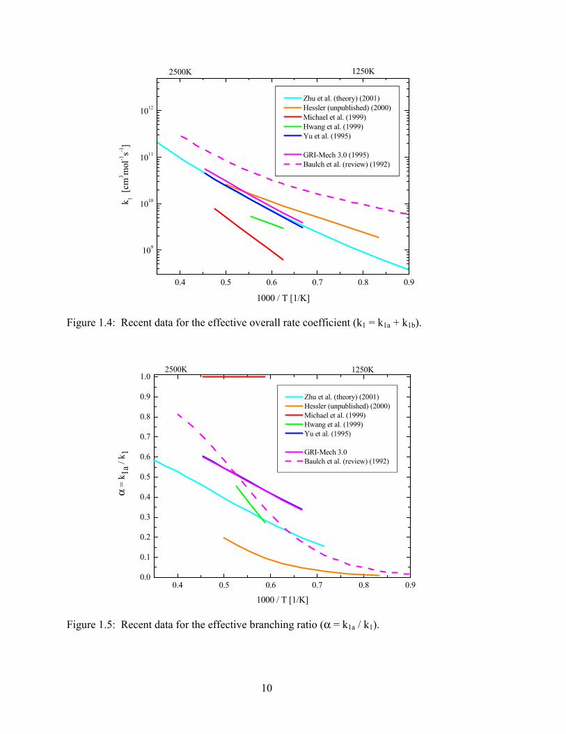
Figure 1.4: Recent data for the effective overall rate coefficient (k1 = k1a + k1b). ........... 10

Figure 1.5: Recent data for the effective branching ratio (α = k1a / k1). .......................... 10

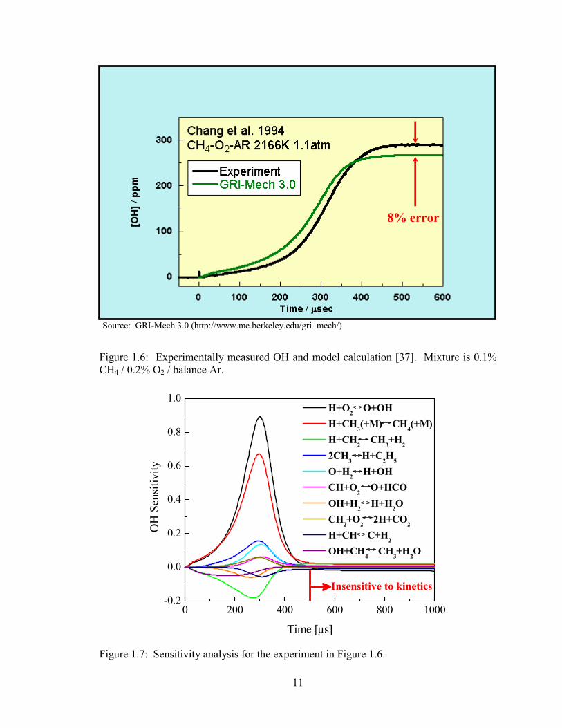
Figure 1.6: Experimentally measured OH and model calculation [37]. Mixture is

0.1% CH4 / 0.2% O2 / balance Ar. ................................................................. 11

Figure 1.7: Sensitivity analysis for the experiment in Figure 1.6. ................................... 11

Figure 2.1: Layout of the OH laser absorption diagnostic. Labeled optics are: (f),

UG-5 Schott glass filter; (l), lens; (i), iris; (NDf), neutral-density filter;

(b1), UV fused silica beam splitter; (b2), 27% beamsplitter; (p), thin-film

polarizer. ........................................................................................................ 27

Figure 2.2: OH absorption reference cell. ........................................................................ 27

Figure 2.3: O-atom ARAS diagnostic layout. .................................................................. 28

Figure 2.4: O-atom ARAS calibration curve. Only a fraction of the complete data

traces are shown here as symbols. Solid line is a zero-constrained 5th-

order polynomial fit to all data....................................................................... 28

Figure 3.1: Brute force sensitivity analysis for OH experiments at T = 1800 K, P =

1.4 atm using GRI-Mech 3.0 with the new values for k1a and k1b.

Mixture is 16 ppm CH3I / 6.25% O2 / 10% He / Ar....................................... 52

Figure 3.2: O-atom sensitivity analysis at T = 1800 K, P = 1.4 atm using GRI-Mech

3.0 with the new values for k1a and k1b. Mixture is 5 ppm CH3I / 1.5%

O2 / 10% He / Ar. The six most sensitive reactions are shown..................... 52

xiv

Figure 3.3: A typical pressure trace from a shock tube measurement. Calculated

conditions are T5 = 1811 K, P5 = 1.42 atm. ................................................... 53

Figure 3.4: Raw data for an OH absorption experiment, showing the reference (Io)

and transmitted (Itrans) signals. The reference signal has been offset for

the purpose of clarity...................................................................................... 53

Figure 3.5: OH absorbance trace resulting from the raw signals in Fig. 3.4.................... 54

Figure 3.6: An example OH experiment at T = 1806 K, P = 1.41 atm, derived from

the traces in Figs. 3.4 and 3.5. Mixture is 16.1 ppm CH3I / 6.28% O2 /

10.2% He / Ar. Calculated lines: bold solid line, k1 = 1.05x1010

cm3mol-1s-1 and k1a = 2.35x109 cm3mol-1s-1 (α = 0.225) to fit both the

OH rise time and subsequent O-atom measurements; bold dashed lines,

k1 ± 25%......................................................................................................... 54

Figure 3.7: PMT output signal from an ARAS measurement. The absorption by O2

is evident immediately behind the incident and reflected shock waves. ....... 55

Figure 3.8: The raw signal from Fig. 3.7 converted into absorbance. Absorption by

O2 at the initial conditions has been accounted for through adjustment of

the baseline..................................................................................................... 55

Figure 3.9: An example O-atom experiment at T = 1846 K, P = 1.34 atm, derived

from the traces in Figs. 3.7 and 3.8. Mixture is 5.14 ppm CH3I / 1.51%

O2 / 10.0% He / Ar. Calculated lines: bold solid line, k1 = 1.35x1010

cm3mol-1s-1 and k1a = 3.45x109 cm3mol-1s-1 (α = 0.255) to fit both the O-

atom experiment and earlier OH rise time measurements; bold dashed

lines, k1a ± 25%. ............................................................................................. 56

Figure 3.10: The experiment from Fig. 3.9, extended out to 1 ms of test time. The

model captures the shifts in the curvature of the O-atom mole fraction

growth, even as sensitivity to secondary chemistry causes slight

deviations in the traces at long test times....................................................... 56

Figure 3.11: Comparison of the present overall rate coefficient k1, open squares and

solid line, to other recent determinations. ...................................................... 57

Figure 3.12: Comparison of the present rate coefficient k1a, open squares and solid

line, to other recent determinations................................................................ 57

xv

Figure 3.13: Comparison of measured OH peak concentrations to model

calculations..................................................................................................... 58

Figure 3.14: Secondary reaction sensitivities at the OH peak concentration................... 58

Figure 4.1: Experimentally measured and modeled OH mole fraction time-histories.

Conditions are T5 = 2590 K, P5 = 1.075 atm, and the mixture is 4002

ppm H2 / 3999 ppm O2 / balance Ar. The OH concentration is modeled

using GRI-Mech 3.0 and the GRI-Mech 3.0 thermodynamics database,

with 0.5ppm additional H-atoms to match the induction time. The fit

required a change in ∆fH°298(OH) from 9.403 to 8.887 kcal/mol. ................. 69

Figure 4.2: Uncertainty analysis for the experiment in Fig. 4.1. Individual error

sources were applied one at a time, and their effect on ΧOH(model) vs.

ΧOH(measured) was noted. The total combined uncertainty in ΧOH was

then used to determine an uncertainty in ∆fH°298(OH) for this

experiment. All other kinetic rate coefficients (not shown here) gave

uncertainties in ∆fH°298(OH) of less than ± 0.0012 kcal/mol. The

combined uncertainties in ΧOH,peak are +2.40% / -2.55%, which translates

into ∆fH°298(OH) = 8.89 +0.15 / -0.14 [kcal/mol].......................................... 70

Figure 4.3: Uncertainty analysis for a low temperature experiment. Conditions are

T5 = 1999 K, P5 = 1.272 atm, and the mixture is 4026 ppm H2 / 4024

ppm O2 / balance Ar. The combined uncertainties in ΧOH,peak are +2.98%

/ -3.06%, which translates into ∆fH°298(OH) = 8.92 +0.14 / -0.13

[kcal/mol]. ...................................................................................................... 71

Figure 4.4: Uncertainty in the measurement of ∆fH°298(OH) due to kinetic rate

coefficient uncertainties. The five most significant reactions are shown.

The increase in OH plateau sensitivity to several reactions effectively

places a low-temperature limit on the current measurement scheme. ........... 72

Figure 4.5: Experimentally derived values for ∆fH°298(OH). (�): Current data;

Solid line: Mean of current data, ∆fH°298(OH)=8.92 [kcal/mol].

Standard deviation from the mean is σ = 0.04. Previous values are given

for reference. .................................................................................................. 73

xvi

Figure 4.6: Change in the measured ∆fH°298(OH) values when the data is reduced

using two additional thermodynamic databases. Data in Fig. 4.5 was

reduced using the GRI-Mech 3.0 thermodynamic database [37]. (�):

Chemkin thermodynamics database [82]; (�): Burcat database [83]. ......... 73

Figure B.1: Effects of collision shift on the line-center absorption coefficient. ............ 118

Figure B.2: Condition space for existing measurements of OH collision shift. Solid

line: P1(2) line in the (0,0) band, Ar and N2 as well as other collision

partners [104]; (�): (0,0) band head [106]; (� and dotted line): (1,0)

band, H2O and N2 collision partners [104]. ................................................. 118

Figure B.3: Experimental setup for collision shift measurements, including the

shock tube and scanning laser diagnostic. ................................................... 119

Figure B.4: Example experimental data for the R1(5) and R21(5) absorption

transitions. Conditions are T5 = 2525 K, P5 = 2.07 atm.............................. 120

Figure B.5: Fit of etalon transmission peaks to transfer measured spectral

information from time-basis to frequency-basis. Successive transmission

peaks have 2 GHz spacing (4 GHz in the UV). Sinusoidal (previous

work) and polynomial (present work) functions have been used to fit the

data. .............................................................................................................. 121

Figure B.6: Example experiment for the R1(5) transition. Conditions are T5 = 2525

K, P5 = 2.07 atm. Only a fraction of the data points are shown for

clarity. The residuals show clear evidence of motional narrowing. In

addition, the asymmetric behavior in the wings of the shock tube

lineshape residual can be observed. ............................................................. 122

Figure B.7: Collision shift data for the R1(5) transition of OH. (�): P5 = 1.5-2.7

atm; (�): P5 = 4 atm; (�): P5 = 7.5 atm. Linear fit of all data yields δAr

= -0.0085* exp(2500/T)0.76 cm-1atm-1 for this transition.............................. 123

Figure B.8: Collision shift data for the R21(5) transition of OH. (�): P5 = 1.5-2.7

atm; (�): P5 = 4 atm; (�): P5 = 7.5 atm. Linear fit of all data yields δAr

= -0.0081* exp(2500/T)0.84 cm-1atm-1 for this transition.............................. 123

Figure B.9: Collision shift data for the P1(1) and P1(2) transitions of OH in Ar. (�):

P1(1) data of current study; (�): estimated P1(2) data of current study;

xvii

(▲): room temperature P1(2) data from [104]. Linear fit of all P1(2)

data (dashed line) yields δAr = -0.0054*exp(2500/T)0.81 cm-1atm-1 for

this transition................................................................................................ 124

Figure B.10: Collision shift data for the P1(1) and P1(2) transitions of OH in N2.

(�): P1(1) data of current study; (�): estimated P1(2) data of current

study; (▲): room temperature P1(2) data from [104]. Linear fit of all

P1(2) data yields δN2 = -0.0045* exp(2500/T)0.55 cm-1atm-1 for this

transition....................................................................................................... 124

Figure B.11: Collision shift coefficients for OH in Ar bath gas, normalized to 2500

K. Symbols for different rotational branches are: (�): R1; (�): R21;

(�): R2; (▲): Q1; (�): Q21. Excluding the Q1 branch, the average

change in collision shift with increasing J” is 4x10-4 ± 4x10-5

[cm-1atm-1/J”]. ............................................................................................. 125

Figure B.12: Collision shift coefficients for OH in N2 bath gas, normalized to 2500

K. Symbols for different rotational branches are: (�): R1; (�): R21;

(▲): Q1; (�): Q21. Excluding the R21 branch, the average change in

collision shift with increasing J” is 3x10-4 ± 1x10-4 [cm-1atm-1/J”]. .......... 125

Figure B.13: Collision-broadening data for the R1(5) transition in Ar. (�): P5 = 1.5-

2.7 atm; (�): P5 = 4 atm; (�): P5 = 7.5 atm; (▲): room-temperature

data from [104]. Solid line is a fit to present data only; dashed line

includes data from [104]. ............................................................................. 126

Figure B.14: Progressive lineshape fits for the R2(7) line in Ar at 2530 K, 2.08 atm.

In this example, assumption of the Voigt profile underestimates the

actual normalized collision shift parameter (s) and Voigt broadening

parameter (y) by 11.6% each........................................................................ 127

Figure C.1: A shock tube experiment to determine the variation in PZT rise times at

the interval timer trigger-threshold voltage. All five transducers are

located in the same plane perpendicular to the axis of the shock tube.

The inset shows the pressure rise from initial to incident shock pressures.

The trigger threshold is typically set to ~10% of the incident pressure

rise. ............................................................................................................... 136

xviii

Figure C.2: An example shock velocity measurement and calculated uncertainties. .... 136

Figure D.1: Emission spectrum of the O-atom ARAS lamp configuration. Operation

parameters were: gas mixture, 1% O2 / He; microwave power, ~70 W;

pressure, 6 torr. Monochromator slits were set to 100 µm for this scan..... 152

Figure D.2: Close-up of the O-atom multiplet from Fig. D.1. ....................................... 152

Figure D.3: Experimental ARAS calibration curve compared to calculations using

the two-layer model. Solid line and symbols: experimental data and

polynomial fit; dashed line: model fit at 2000K; dotted lines: model

calculations for 1600 K and 2400 K using the same assumed lamp

parameters. ................................................................................................... 153

Figure D.4: Effects of lamp self-absorption and line reversal on the emission

lineshape....................................................................................................... 153

Figure E.1: Chemkin calculation for comparison to the partial equilibrium model.

Conditions are 2500 K, 1 atm with a mixture of 0.4% H2 / 0.4% O2 / Ar.

Mechanism is from Masten [130] and thermodynamic data from Kee et

al. [82]. ......................................................................................................... 159

Figure E.2: Sensitivity calculations for the conditions of Fig. E.1. ............................... 159

1

Chapter 1: Introduction

1.1 Motivation Modern combustion systems are ideally designed to achieve high thermal

efficiency and low pollutant emissions, while the end users of these systems are

additionally interested in high reliability and the lowest obtainable cycle cost necessary to

produce the desired propulsive force, mechanical motion, electricity, or heat. The

development of combustion systems is greatly enhanced by accurate detailed models and

computational methods which can predict, with high confidence, how a proposed design

will function and how perturbations to the design can lead to an optimization of its

performance. Models for combustion systems typically incorporate information about

combustion chemistry, fluid dynamics, and heat transfer. Because of the complex

physical nature of combusting matter, particularly in turbulent flows, combustion

chemical kinetic mechanisms assembled for computational purposes are often simplified

or “reduced” to improve computational efficiency while still reproducing the most critical

features of the fully detailed model – features such as autoignition time, flame speed, or

pollutant formation characteristics. These reduced mechanisms, however, can only be as

accurate as the fully detailed mechanisms or experimental data on which they are based,

and they are somewhat limited in application to the specific combustion environment or

combustion parameters for which they are optimized.

Accurate, predictive detailed combustion chemistry mechanisms require 3 major

components: 1) a complete set of reactions, 2) reaction rate coefficients for every

reaction (with accurate rate expressions for the most important reactions), and 3)

thermodynamic and thermochemical data for each species, along with the complete

temperature and pressure dependence for (2) and (3). The mechanisms’ success in

recreating real combustion phenomena is largely dependent on careful experimental

determinations of rate coefficient and thermochemical parameters of the reactions and

2

species in the model. In addition, theoretical calculations are increasingly a vital part of

this process. As theoretical methods are validated by prudent experimental

measurements, confidence is gained in the theory, which can then be pushed farther and

faster to explore model parameters which are difficult or impossible to determine

experimentally. Until the time that theoretical methods are unwaveringly accurate,

however, well-thought-out experimental determination of critical combustion parameters

will be an essential means by which to improve the accuracy of combustion chemical

kinetic mechanisms.

In this thesis work, a shock tube has been used to perform carefully designed

measurements of combustion chemical kinetic and thermochemical parameters. Two

specific projects are highlighted here: a measurement of the reaction rate of CH3+O2→

products, an important reaction in the combustion of natural gas and other hydrocarbon

fuels; and a high-temperature determination of the standard heat of formation of the

hydroxyl radical (OH) at 298 K, ∆fH°298(OH). Supporting work has also been performed

which enhances the reliability of the spectroscopic diagnostics and experimental methods

used in this investigation.

1.2 Background

1.2.1 CH3+O2→products

The reaction of methyl radicals with molecular oxygen plays a role in the

oxidation of many alkanes, and is often the rate-controlling reaction during the methane

(CH4) ignition process under radical-lean combustion conditions. The three well-known

product channels are:

CH3 + O2 → CH3O + O (1a)

→ CH2O + OH (1b)

(+M) → CH3O2 (+M) (1c)

Channels (1a) and (1b) are the dominant reaction pathways at combustion temperatures,

and channel (1c) is thought to become important below 1500 K as well as at higher

pressures [1]. Figure 1.1 shows the sensitivity of CH4 ignition times to these and other

reactions.

3

Due to the importance of the CH3 + O2 reaction in hydrocarbon oxidation, it has

been the focus of numerous experimental [2-24] and theoretical [1,11,24-27]

investigations. The published rate coefficient values are plotted in Figs. 1.2 and 1.3.

Shock tube experimental studies have ranged from CH4 oxidation [4-

6,9,12,14,17,18,21,22,24] to ultra-lean experiments using CH3 precursors such as methyl

iodide (CH3I) [16,19], azomethane ((CH3)2N2) [7,8,11,13,15,23], and ethane (C2H6)

[3,13,19]. The diagnostics utilized include optical absorption of OH [4,5,7,12,19,24],

CH3 [12], CO [11,23,24], H2O [23], N2O [4], CH4 [18], and H- [3,15,17,19] and O-atoms

[3,15-17,19]; optical emission of OH [4], CO [9,13], and CO2 [9,13]; CO flame band

emission [5,6,14]; post-shock density gradients [21]; pressure [4]; and time-of-flight mass

spectrometry [8]. Other experimental work includes flow reactor studies [10,20] and

Knudsen cell experiments [2] utilizing mass spectrometry. In spite of the effort devoted

to studying this reaction, there remains disagreement regarding the overall rate

coefficient, k1 = k1a + k1b, and the individual rate coefficients of the two major product

channels at combustion temperatures.

As discussed in Hwang et al. [12], early studies suffered from the lack of accurate

knowledge of, and sometimes exclusion of, important secondary chemistry. Experiments

were performed with the expectation of chemical isolation, when in fact the measured

results were influenced by chemistry in addition to reaction (1). Aside from secondary

chemistry, Yu et al. [24] point out that the a priori assumption of dominance of either

channel (1a) or (1b) influenced the rate coefficients reported for these reactions. Michael

et al. [16] note that the yields of some species, such as OH and CO, in CH4 ignition

experiments are somewhat insensitive to whether the initial reaction pathway proceeds

through channel (1a) or (1b). Consequently, investigations purporting to measure one or

the other could not always discern which reaction they were in fact measuring, and most

likely they were observing the combined effects of both channels. For these reasons, and

due to the complexity of the subsequent secondary chemistry, previous experimental

studies have resulted in reaction rate coefficients for channels (1a) and (1b) which span

more than a factor of four and over an order of magnitude, respectively.

Even the most recent high-temperature studies, including three experimental

studies and one theoretical calculation, have not provided consensus values for the

4

overall rate and branching ratio, α = k1a/k1. Figures 1.4 and 1.5 display the effective

overall rate and branching ratio from high-temperature studies in only the last 10 years.

The study of Yu et al. [24] utilized measurements of OH and CO rise times in lean CH4

ignition experiments. Starting with a theoretical calculation for k1b (which was fit, in

part, to data from two earlier studies [2,10]), these workers fit their experimental data by

fixing k1b to the calculated value and adjusting k1a. The final experimental expression for

k1a was found to compare favorably to their theoretical calculation of that channel.

Michael et al. [16] measured O-atom concentrations in ultra-lean CH3I / O2 experiments

and reported that, for temperatures between 1600 and 2100K, reaction (1a) is the only

significant channel and that the rate of this reaction is substantially lower than that

reported by Yu et al. In addition, Michael et al. were unable to fit their O-atom data if

channel (1b) was included in the model. Hwang et al. [12] measured OH and CH3 in lean

CH4 ignition experiments similar to those of Yu et al. They reported a rate coefficient for

channel (1a) that is in close agreement with Michael et al., but they found that the rate of

channel (1b) could not be reduced to zero. Recent ab initio calculations of Zhu et al. [1]

agree with the overall rate of Yu et al. to within 10% in their overlapping temperature

range, but the calculated branching ratio α is approximately 25% to 45% lower. Among

these most recent studies, k1a has a spread of a factor of ~3 and k1b ranges from being

dominant to being negligible.

Given the lack of agreement among recent studies, a shock tube study of the

reaction CH3+O2 → products was undertaken using cw laser absorption spectroscopy of

OH and O-atom atomic resonance absorption spectroscopy (ARAS) measurements. This

study was designed to overcome many of the obstacles which have previously prevented

actual experimental determination of both high-temperature channels within one study,

and it provides a self-consistent basis for comparison to measurements from other

laboratories.

1.2.2 The heat of formation of OH

Detailed chemical kinetics models for combustion and atmospheric chemistry

require not only chemical reactions and their rate coefficients, but also accurate

thermochemical and thermodynamic parameters for all species involved. Incorrect

5

thermochemical data can lead to erroneous kinetic modeling via calculation of reverse

rate coefficients through the equilibrium constant. Accurate thermochemical parameters,

particularly the heat of formation, are typically difficult to measure or calculate directly,

and species for which the uncertainties in thermochemical parameters are small enough to

be ignored in combustion modeling are very few [28]. Parameters for radical species, in

particular, are difficult to obtain due to their reactivity and small concentrations at

convenient experimental conditions. Because of the importance of radicals, such as OH,

in the ignition process of all fuels and in atmospheric chemistry, accurate thermochemical

parameters must be used to correctly model the chemistry.

Recently, renewed attention has been given to the heat of formation of the OH

radical. Ruscic et al. [29,30] have suggested that the generally accepted standard heat of

formation of OH at 0 K, ∆fH°0(OH) = 9.35 kcal/mol [31] or ∆fH°0(OH) = 9.18 kcal/mol

[32], is too high by up to 0.5 kcal/mol, based on both new experimental measurements of

the OH positive-ion cycle and ab-initio electronic structure calculations. These authors

provide an in-depth analysis of past determinations of the heat of formation of OH and

the two successive bond dissociation energies of water, D0(H-OH) and D0(O-H). The

previously accepted value for ∆fH°0(OH) is based on a value of the dissociation energy of

OH, D0(O-H), determined from a short Birge-Sponer extrapolation [33] of the potential

energy surface from spectroscopically measured vibrational energy levels [34]. Through

their analysis, Ruscic et al. show that the Birge-Sponer extrapolation, while very short

(~1.5 vibrational levels), has significant errors leading to an underprediction of D0(O-H)

and therefore an overprediction of ∆fH°0(OH). In another recent paper, Joens [35] used

available experimental data and thermochemical cycles of H2O and H2O2 to infer a value

for ∆fH°0(OH) in essential agreement with Ruscic et al. [29,30]. These recent studies

highlight the previous methods that have been used to determine the heat of formation.

The present study of the heat of formation of OH was motivated by these recent

results and the impact that such a change in a fundamental thermochemical parameter

like ∆fH°0(OH) would have on other thermochemical parameters and many combustion

and atmospheric chemistry reactions. An additional motivation was that experiments in

our own laboratory of shock-initiated combustion of CH4/O2 and C2H6/O2 mixtures

[36,37] have revealed that kinetic models consistently underpredict the OH concentration

6

in the post-ignition plateau region by as much as 10-15%. An example of such an

experiment is shown in Fig. 1.6. This amount of discrepancy for an OH laser absorption

measurement is alarming, as the diagnostic is highly quantitative and OH measurements

are considered to be better than ±3% accurate at these conditions. The discrepancy

indicates that either 1) the diagnostic has significant unforeseen errors or 2) the plateau is

sensitive to an erroneous thermochemical parameter which controls the plateau

concentration of OH.

Hypothesis (1) has been investigated here through a careful evaluation and review

of the spectroscopic information used in the calculation of absorption coefficients, as well

as further measurements of OH lineshape collision broadening and collision shift

parameters. Through these investigations, the methods and parameters for calculation of

OH spectral absorption coefficients have been updated and improved. However, these

improvements do not go far enough to explain the OH plateau discrepancy.

Hypothesis (2) draws from the fact that the sensitivity of OH plateaus to kinetic

rate parameters is very small compared to the sensitivity to thermochemical parameters,

particularly the heat of formation of OH. Figure 1.7 is a kinetic sensitivity analysis for

the experiment in Fig. 1.6. In the plateau region, the sensitivity to all reaction rates is

essentially zero, and the plateau concentrations are wholly controlled by the

thermochemical parameters of the species involved in the partial equilibrium plateau. Of

these species, the thermochemistry of OH is the most in question. The discrepancy in the

plateau OH concentration thus represents an opportunity to perform measurements of the

heat of formation of OH. This work details the experimental planning and results of an

independent determination of ∆fH°298(OH) using shock-heated mixtures of H2 and O2.

1.3 Scope and organization of thesis The objectives of this research were: 1) to design and perform high-precision,

low-uncertainty measurements of the overall reaction rate of CH3+O2→products and to

determine the rates for the individual product channels, 2) to perform unique high-

temperature measurements of the heat of formation of OH, and 3) to enhance the

reliability of the diagnostics and shock tube techniques utilized for these and future

combustion chemistry measurements.

7

Chapter 2 describes the experimental apparatus and diagnostic techniques used in

this work. Information is presented regarding the shock tube facility, equipment, and

design changes implemented to improve the facility and enable sensitive measurements

using low concentration mixtures. The OH laser absorption diagnostic is discussed. An

apparatus for O-atom measurement using the ARAS technique was built, characterized,

and calibrated for use in kinetics experiments and is described here.

Chapters 3 and 4 contain the primary experimental work in this thesis. The

investigation of the reaction CH3+O2→products is presented in Chapter 3. This chapter

describes the unique approach developed to experimentally determine the individual

product channels. The design of experiments, results, and uncertainty analysis are given.

Chapter 4 details the high-temperature measurement of the heat of formation of OH. The

results, their comparison to other recent determinations, and a detailed uncertainty

analysis are provided. Chapter 5 concludes with suggestions for ongoing work in related

topic areas.

An important review of OH spectroscopy and the calculation of spectral

absorption coefficients is given in Appendix A. Measurements of OH lineshape

collision-shift and collision-broadening parameters are presented in Appendix B.

Appendix C details an uncertainty analysis for the calculation of the temperature and

pressure behind the reflected shock wave, based on uncertainties in the incident shock

velocity and initial conditions. Appendix D gives further details on the ARAS technique.

Appendix E is a discussion of the partial equilibrium state in H2/O2 mixtures which is

used to determine the heat of formation of OH.

8

Figure 1.1: Sensitivity of CH4 ignition times to various reactions [37]. Mixture is 9.1% CH4 / 18.2% O2 / Ar. Conditions are 1500 K, 1.8 atm.

Sensitivity of τign to reaction rates Source: GRI-Mech 3.0 (http://www.me.berkeley.edu/gri_mech/)

9

0.4 0.6 0.8 1.0 1.2106

107

108

109

1010

1011

Zhu et al. (2001) Hessler (unpublished) (2000) Michael et al. (1999) Hwang et al. (1999) Yu et al. (1995) Braun-Unkhoff et al. (1993) Klatt et al. (1991) Wu et al. (1990) Zellner and Ewig (1988) Dean and Westmoreland (1987) Saito et al. (1986) Hsu et al. (1983) Bhaskaran et al. (1980) Teitelboim et al. (1978) Brabbs and Brokaw (1975)

Baulch et al. (review) (1992) GRI-Mech 3.0

k 1a [c

m3 m

ol-1

s-1]

1000/T [1/K]

Figure 1.2: Previous rate coefficient data for k1a.

0.4 0.6 0.8 1.0 1.2108

109

1010

1011

1012 Zhu et al. (2001) Scire et al. (2001) Hessler (unpublished) (2000) Yu et al. (1995) Braun-Unkhoff et al. (1993) Grela et al. (1992) Zellner and Ewig (1988) Saito et al. (1986) Hsu et al. (1983) Borisov et al. (1981) Bhaskaran et al. (1980) Tabayashi and Bauer (1979) Olson and Gardiner (1978) Baldwin and Golden (1978) Teitelboim et al. (1978) Tsuboi (1976) Bowman (1975) Jachimowski (1974) Dean and Kistiakowsky (1971) Izod et al. (1971) Clark et al. (1971)

Baulch et al. (review) (1992) GRI-Mech 3.0

k 1b [c

m3 m

ol-1s-1

]

1000/T [1/K]

Figure 1.3: Previous rate coefficient data for k1b.

10

0.4 0.5 0.6 0.7 0.8 0.9

109

1010

1011

1012

Zhu et al. (theory) (2001) Hessler (unpublished) (2000) Michael et al. (1999) Hwang et al. (1999) Yu et al. (1995)

GRI-Mech 3.0 (1995) Baulch et al. (review) (1992)

1250K

k 1 [cm

3 mol

-1s-1

]

1000 / T [1/K]

2500K

Figure 1.4: Recent data for the effective overall rate coefficient (k1 = k1a + k1b).

0.4 0.5 0.6 0.7 0.8 0.90.0

0.1

0.2

0.3

0.4

0.5

0.6

0.7

0.8

0.9

1.0

Zhu et al. (theory) (2001) Hessler (unpublished) (2000) Michael et al. (1999) Hwang et al. (1999) Yu et al. (1995)

GRI-Mech 3.0 Baulch et al. (review) (1992)

1250K

α =

k 1a /

k 1

1000 / T [1/K]

2500K

Figure 1.5: Recent data for the effective branching ratio (α = k1a / k1).

11

Figure 1.6: Experimentally measured OH and model calculatioCH4 / 0.2% O2 / balance Ar.

0 200 400 600 8-0.2

0.0

0.2

0.4

0.6

0.8

1.0

OH

Sen

sitiv

ity

Time [µs]

H+O2 O+O H+CH3(+M) H+CH2 CH 2CH3 H+C O+H2 H+O CH+O2 O+ OH+H2 H+ CH2+O2 2H H+CH C+H OH+CH4 C

Insensitive

Figure 1.7: Sensitivity analysis for the experiment in Figure 1.6

Source: GRI-Mech 3.0 (http://www.me.berkeley.edu/gri_mech/)
8% error
n [37]. Mixture is 0.1%

00 1000

H CH4(+M)

3+H2

2H5

HHCOH2O+CO2

2

H3+H2O

to kinetics

.

13

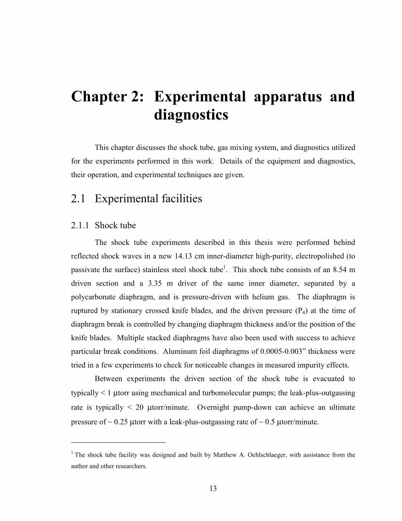
Chapter 2: Experimental apparatus and diagnostics

This chapter discusses the shock tube, gas mixing system, and diagnostics utilized

for the experiments performed in this work. Details of the equipment and diagnostics,

their operation, and experimental techniques are given.

2.1 Experimental facilities

2.1.1 Shock tube

The shock tube experiments described in this thesis were performed behind

reflected shock waves in a new 14.13 cm inner-diameter high-purity, electropolished (to

passivate the surface) stainless steel shock tube1. This shock tube consists of an 8.54 m

driven section and a 3.35 m driver of the same inner diameter, separated by a

polycarbonate diaphragm, and is pressure-driven with helium gas. The diaphragm is

ruptured by stationary crossed knife blades, and the driven pressure (P4) at the time of

diaphragm break is controlled by changing diaphragm thickness and/or the position of the

knife blades. Multiple stacked diaphragms have also been used with success to achieve

particular break conditions. Aluminum foil diaphragms of 0.0005-0.003” thickness were

tried in a few experiments to check for noticeable changes in measured impurity effects.

Between experiments the driven section of the shock tube is evacuated to

typically < 1 µtorr using mechanical and turbomolecular pumps; the leak-plus-outgassing

rate is typically < 20 µtorr/minute. Overnight pump-down can achieve an ultimate

pressure of ~ 0.25 µtorr with a leak-plus-outgassing rate of ~ 0.5 µtorr/minute.

1 The shock tube facility was designed and built by Matthew A. Oehlschlaeger, with assistance from the

author and other researchers.

14

Shock velocity is measured using five axially spaced PCB Piezotronics 113A26

piezoelectric transducers (PZT’s) and a 6-channel amplifier (PCB 483B08) connected to

four Philips PM6666 interval timers with a resolution of 0.1 µs. The shock trajectory is

fit to the velocity data using a linear attenuation profile and extrapolated to the endwall;

the typical incident-shock attenuation rate for Ar bath gas is 1-1.5 %/m. Post-shock

conditions are calculated from the extrapolated endwall shock velocity, initial pressure,

and initial temperature using standard shock wave relations and assuming chemically

frozen and vibrationally equilibrated gases. For some of the work in this dissertation,

vibrational equilibration cannot necessarily be assumed without careful consideration of

the characteristic vibrational relaxation times of the mixture. Uncertainty in the

calculation of the initial reflected-shock temperature and pressure (T5 and P5) is typically

on the order of 0.7% and 1%, respectively. An uncertainty analysis for T5 and P5 is

provided in Appendix C.

The post-shock gases are optically accessed through 0.75” diameter windows

centered 2 cm from the endwall and mounted flush to the inner radius of the shock tube.

For OH laser absorption experiments, the window material was typically sapphire, UV

fused silica, or CaF2 with a nominal thickness of 0.125”. A fifth PZT, Kistler model

603B1 with model 5010B amplifier, is mounted at this same axial location and is used to

measure the pressure-time history of the experiment. All PZT’s are recessed ≈ 1 mm

from the inner diameter surface and coated with 1 mm of red silicone RTV to protect

them from thermal shock and temperature-induced changes in their sensitivity.

The shock tube’s driven section was occasionally cleaned using clean cloth rags

and methanol. During the kinetics work discussed in Chapter 3, ultra-high-purity gases

and very low reactant concentrations were used in the gas mixtures; therefore cleaning

was performed sparingly and usually not until the presence of diaphragm particles in the

test section began to disturb the measurements. Following a cleaning the shock tube

must be evacuated to high vacuum overnight to remove residual solvent and water vapor

from the shock tube walls. Typically the first three to five shocks were run with pure Ar

or pure O2 at very high temperatures to assist in driving the remaining solvent off of the

walls and removing it during the pump-down cycle.

15

2.1.2 Gas mixing facility

Gas mixtures were prepared manometrically in a 12-liter stainless steel and

aluminum mixing cylinder and mechanically mixed with a magnetically driven stirrer.

Gases were connected to the mixing cylinder, vacuum system, and shock tube via a

stainless steel welded-tubing manifold with stainless steel bellows-sealed valves. Gas

pressures were measured using high-accuracy MKS Baratron 690A capacitance

manometers with MKS 270D signal conditioner / display readouts. Two transducers,

with useful ranges of 100 torr and 10,000 torr, are connected to the manifold and permit

accurate and precise measurement of the minor constituents as well as the final mixture

pressure. The same transducers are also utilized for measurement of the pre-shock

pressure in the driven section, P1. A Varian ionization pressure gauge is mounted to the

vacuum manifold for measurement of high vacuum during pump-down of the mixing

system. A Setra 280E capacitance pressure transducer is mounted directly to the mixing

cylinder in order to provide full-time measurement of the tank pressure. During mixture

preparation, even with slow filling rates, the gases in the cylinder become slightly heated.

Typically the final pressure of the mixture will drop 0.3-0.5% over the first hour or two

of mixing as the gases cool down. This sensor enables monitoring of the cool-down

process and the final equilibrated mixture pressure, and is a constant measure of the

remaining gas mixture pressure during sets of shock tube experiments.

The gas manifold, mixing cylinder, and all gas lines are evacuated using

mechanical and turbomolecular pumps connected directly to the manifold and cylinder

via 1”-diameter fittings. Previous to the current work, a direct-drive mechanical pump

alone was used to evacuate the mixing cylinder, with an ultimate vacuum pressure limit

of > 1 mtorr. Addition of the turbomolecular pump, along with design changes that

shortened the length and increased the diameter of all vacuum lines, both increased

effective pumping speed and decreased the ultimate pressure. Shock wave experiments

performed before and after the mechanical changes confirmed a significant improvement

in residual impurities and, therefore, the ability to make accurate low-concentration gas

mixtures. The mixing cylinder can be evacuated to ~ 2 µtorr overnight, with leak-plus-

outgassing rates of ~ 100 µtorr/minute. Less than 1 µtorr can be achieved after 2-3 days,

with the lowest recorded pressure of 0.63 µtorr and leak-plus-outgassing rate of 8.6

16

µtorr/minute after more than one week of pumping. The manifold alone, without the

mixing cylinder, is routinely pumped down to < 1 µtorr between experiments.

2.1.3 Mixture preparation

One goal in designing the mixture preparation procedure is to minimize

uncertainties stemming from the measurement of gas pressures. The combination of 100-

torr and 10,000-torr capacitance manometers was chosen in large part due to the

requirements of this work. The ultra-low-concentration mixtures used for the chemical

kinetics experiments in Chapter 3 were prepared using a double dilution process, whereas

higher-concentration mixtures in Chapter 4 were prepared in a single dilution. Mixture

preparation procedures were kept as consistent as possible from mixture to mixture.

The methyl precursor used in these experiments, methyl iodide (CH3I), was

99.5% pure and is commonly available from chemical suppliers. It has a vapor pressure

of ~ 400 torr at room temperature. Methyl iodide is a toxic substance, so caution must be

observed in its handling.

Samples of CH3I were prepared inside a fume hood by pouring the desired

amount of liquid into a glass flask with a sealing valve, such as the Airfree® type made

by Chemglass, Inc. The valve is closed, and liquid remaining above the valve is removed

by pumping it out with a vacuum line. The flask is then taken from the fume hood and

connected to the shock tube mixing manifold. Before making a mixture, the air and any

other high-volatility compounds must be removed from the flask through a freeze-pump-

thaw cycle. A bath of liquid nitrogen (LN2) is used during this process to cool down the

flask and the liquid inside. Once it starts to cool, the flask is opened up to the mixing

manifold and the mechanical pump is used to evacuate the gases while further cooling the

liquid to the frozen state. Typically some amount of cavitation is visible as air and other

gases come out of solution in the liquid, until eventually the liquid is frozen solid. At this

point the turbomolecular pump can be activated and the pressure in the system decreases

to < 10 µtorr. After reaching a stable vacuum, the LN2 is removed and the liquid is

allowed to slowly warm up. The flask valve can be shut once the pressure reaches a few

hundred µtorr. As the frozen CH3I becomes liquid, if bubbles are seen escaping the

liquid, this is an indication that some high-volatility gases were still trapped in the solid

17

phase, and the freeze-pump-thaw cycle should be repeated until no such bubbles are seen

upon thawing of the solid. Following preparation of the sample, the liquid should be

shielded from all light sources to slow down the photolytic decomposition of CH3I. After

a few days, if the sample has a yellow tint, this is an indication that some amount of

decomposition has occurred. The sample should be disposed of, the flask rinsed out, and

a new sample should be prepared.

A new gas mixture is prepared once the mixing manifold and tank have been

evacuated to a satisfactory vacuum, usually after a minimum of 12 hours of

turbopumping. The steps for making a 5ppm CH3I / 1.5% O2 / 10% He / balance Ar

mixture are shown in Table 2.1. During the entire process, the mechanical stirrer is

constantly moving to enhance mixing and reduce stratification of the different component

gases. The primary source of uncertainty in preparing gas mixtures is the accuracy of the

pressure gages. Based on company literature and assuming a room-temperature deviation

of ±2oC, calculated uncertainties in a calibrated Baratron range from 0.13%, 0.16%,

0.43%, and 3.22% of the reading for measurements at full scale (F.S.), 10% F.S., 1%

F.S., and 0.1% F.S., respectively. To minimize uncertainties, the goal is to keep the

smallest pressure measurement as large as possible within the range of the available

gages. To this end, the pressures in steps 1 and 4 are kept fairly close to one another.

Otherwise, one of them will be smaller and incur an increased potential for error. As

mentioned in the previous section, while the high-pressure mixture cools down the

pressure will drop slightly. The tank is closed-off at this point, so the Setra pressure

reading before and after mixing should be noted as an indication of the relative change in

the final pressure reading from steps 2 and 7.

Initially, a short mixing time, ~1-2 hours, was used in step 8. However,

incomplete mixing was suspected due to the initial low OH yields which slowly increased

over the first few shocks of the mixture. Experiments run with mixtures containing C2H6

rather than CH3I gave consistent results, lending confidence that loss of CH3I to wall

adsorption was not a significant problem. Therefore, the conclusion was that the

stratification of the gases during filling and the short mixing time precluded complete

mixing of the gases. The procedure in Table 2.1 was therefore adopted for all low-

concentration experiments in Chapter 3.

18

2.2 OH laser absorption diagnostic Concentration time-histories of OH were measured using cw laser absorption of

transitions in the A-X(0,0) system near 306.7nm. The laser absorption technique for OH

was initially developed in our laboratory [38] and has been steadily improved upon,

including studies of line shape owing to collision broadening [39] and collision shift (see

Appendix B). The R1(5) transition is most commonly used due to its isolated lineshape

and high linestrength over a range of temperatures at typical shock tube conditions,

although other nearby transitions have also been used in this work as a check of the

spectroscopic database and experimental procedures.

2.2.1 Experimental setup

The diagnostic layout is shown in Fig. 2.1. A diode-pumped solid-state laser

(Coherent Verdi or Spectra Physics Millenia at 5W of cw 532nm radiation) is used to

pump a frequency-doubled Spectra Physics 380 dye laser operating on Rhodamine 6G

dye, producing several mW of UV light. Typically 4-6 mW of UV was available,

although anywhere from 7 to more than 10 mW has been achieved. The UV power

output is highly dependent on the age of the dye, condition/cleanliness of the doubling

crystal and other cavity optics, and the configuration, alignment, and focus adjustments

of the cavity optics. While the UV power is sufficient, the laser cavities in use in our

laboratory are nearing 15 to 25 years in age and they are no long capable of producing the

same power levels as when they were new, probably due to aging and obsolete

intracavity optics and cavity mirrors. The laser cavity has been modified by previous

workers to permit rapid-tuning of the laser frequency [40], a feature used in the collision-

shift and -broadening measurements described in Appendix B. Portions of the visible

light output from the cavity are used to monitor laser wavelength, mode quality, and

power. The fundamental laser wavelength is measured with a Burleigh Instruments WA-

1000 Wavemeter®, and the mode quality is visualized using a 2 GHz free spectral range

(FSR) Burleigh Instruments confocal scanning interferometer (spectrum analyzer) and

RC-46 spectrum analyzer controller.

The detection layout at the shock tube is similar to a setup suggested by Petersen

[41] in his high pressure work. Before entering the shock tube, the UV laser output is

19

split into two beams using a beamsplitter with a coating that gives 27% reflection. Each

beam is focused onto a fast-response Silicon photodiode/amplifier package, and the

intensities in the two beams are balanced by adjusting the angle of a neutral density filter

placed in one beam’s path. The balanced signals provide common-mode noise reduction,

typically yielding at least a factor of 10 improvement in RMS baseline noise. Previous

laser absorption designs used uncoated UV fused silica beamsplitters to split off ~5% of

the laser beam before and after the shock tube. The angle of the beamsplitters (and

therefore the collection lens and detector position) were adjusted to balance the detector

signals. The new design has the advantage of decreasing the number of polarization-

sensitive optics on the exit side of the shock tube (much more important in very high

pressure experiments than in the current work), and increasing the laser power on the

detectors. In general, higher laser power on the detectors is always beneficial (up to the

point of damaging the detectors), as it lifts the signal above the noise floor of the

detector/amplifier electronics and permits lower gain/higher bandwidth settings.

Balancing is also made much easier by the angle-adjustment of the neutral density filter,

enabling fine tuning of its fractional transmission. An iris in each beam path blocks

secondary reflections of the laser beam from entering the lens and detector, and Brewster-

angled UG-5 Schott glass filters placed in front of the detector faces reduce noise from

background light sources and shock tube emission. The detector signals are then

digitized and stored for analysis in an 8-channel, 12-bit, 10 MHz sample rate (20 MHz

maximum in single-channel mode) Gagescope data acquisition system and computer.

A low-pressure (~ 25 torr) microwave discharge in a flowing cell of He and water

vapor produces low concentrations of OH and is used as a spectrally unshifted reference

for the line-center absorption wavelength of the desired OH transition. This cell, shown

in detail in Fig. 2.2, was built primarily for use in collision-shift measurements where the

laser wavelength was rapidly tuned over the entire absorption lineshape. It was also

utilized for some fixed-frequency measurements and to check the Wavemeter calibration,

as described below.

The flowing cell is constructed from 0.5” O.D. Pyrex tubing, with O-ring-sealed

“T” fittings at either end. The fittings are machined to Brewster’s angle and U.V. fused

silica windows are epoxied to the fittings to form the ends of the cell. Helium gas at ~1

20

atm flows through a glass saturator (a “bubbler”) containing liquid water and then into

one end of the cell. A vacuum pump constantly evacuates the cell through the other end,

and a needle valve between the saturator and cell controls the pressure in the cell as

measured with an MKS Baratron 100-torr capacitance manometer, model 122AA-

00100AB, and displayed on an MKS PDR-D-1 readout. A ball-type shut-off valve

isolates the cell from the vacuum pump when not in use. The UV beam is sampled

before and after this reference cell and the light is detected by matched UV-enhanced Si

photodiode/amplifier packages.

The reference cell was used in the following manner. In a fixed-frequency

experiment the Wavemeter enables rough tuning of the laser wavelength, while prior to

each experiment the laser is finely tuned (within a laser cavity mode spacing of 0.016

cm-1 in the UV) to the peak absorption in the reference cell. This method provides an

absolute calibration of the laser wavelength at the time of the shock to the (near) vacuum

line-center wavelength of the desired OH transition, νo. The benefit of using the

reference cell is that it eliminates any absolute errors in the Wavemeter reading due to

slight misalignment or poor resolution. If the absorption transition’s line-center

wavelength at shock tube conditions is significantly different than at vacuum, based on

knowledge of the collision shift (see Appendix B), the Wavemeter can be used to make

relative adjustments in the laser wavelength.

The Wavemeter has an estimated uncertainty of ±0.017 cm-1, dominated by the

uncertainty in the reference laser’s wavelength of ±500 MHz [42]. The precision of the

Wavemeter’s readout is 0.01 cm-1. Over several experiments, comparison of the

Wavemeter reading to the known vacuum line-center wavelength (as determined by peak

absorption in the OH reference cell) was typically quite consistent within the Wavemeter

readout precision of ±0.01 cm-1; and after some time the Wavemeter was trusted as the

primary reference. However, caution must be observed during the alignment of the laser

beam into the Wavemeter. Observations confirmed that, for accurate readings, the

incoming beam should be aligned with the output HeNe laser beam over a distance of at

least 1 m before entering the Wavemeter. Slight misalignment, while still enabling the

Wavemeter to produce a reading, can cause errors on the order of 0.01-0.02 cm-1. This

translates into errors of 0.02-0.04 cm-1 in the frequency-doubled laser beam, resulting in

21

potential absorption coefficient errors of up to ~ 6% (at 1800 K, 1.4 atm) if the error is

not accounted for.

2.2.2 OH diagnostic improvements

A few improvements to the laser absorption diagnostic have been implemented

during this work, including a new pump laser, large area detectors, a careful review of the

calculation of spectral absorption coefficients (given in Chapter 3 and Appendix A), and

the diagnostic layout described above. The Coherent Verdi solid-state pump laser has

considerably lower noise, better power stability and pointing stability, and easier day-to-

day operation than the previous Ar+ pump lasers. The improved power stability and

pointing stability, in particular, greatly improve dye laser operation because the incoming

pump beam is stable over time and between activity cycles on different days. The lower

noise spectrum amplitude of the solid-state laser and the absence of the low-frequency

intensity noise often seen on the older Ar+ lasers both translate into lower noise on the

dye laser output beam. This, in turn, results in quieter absorption signals. Measurements

of the two pump laser sources indicated 0.63% RMS noise for the Ar+ laser compared to

0.068% RMS noise for the Coherent Verdi laser. The frequency-doubled dye laser

output, when pumped by each of the lasers and carefully balanced to achieve common-

mode noise rejection, yielded an improvement of more than a factor of 5 in RMS noise in

the pre-shock regime, from 0.38% absorption noise with the Ar+ laser to 0.063% noise

with the new solid-state laser. This RMS noise level represents the detection limit for

OH at a signal/noise ratio of 1. A large portion of this improvement is due to the higher

available laser power from the new solid-state pump laser compared to the aging Ar+

laser.

The change in pump laser sources also affects the performance of the dye. Due to

the higher absorption coefficient of Rhodamine 6G dye (R6G or Rhodamine 590) at 532

nm compared to the multiple wavelengths in the Ar+ pump lasers, the standard dye

concentration should be decreased in order to maintain the desired 80-90% absorption of

the pump beam by the dye jet. This change in dye concentration vs. absorption for the

two pump lasers was verified experimentally by measuring the laser power transmitted

through the dye jet. Pure ethylene glycol was circulated in the laser, and concentrated

22

dye solution was added in steps while the transmitted laser power was observed. The

optimal dye concentrations for 88% absorption in the dye jet were found to be 0.33 g/L

and 0.97 g/L for the 532 nm laser and the multi-line output of the Ar+ laser, respectively.

It should be noted that other dyes and concentrations may be used with success.

For example, increasing the dye concentration will typically red-shift the wavelength

peak of the fluorescence curve. The benefit of shifting the peak must be weighed against

the possibility of decreases in performance and stability as we move away from the

optimum concentration for a given dye/solvent/pump power and wavelength

combination. The best dye selection for a specific application is one which balances high

fluorescence yield at the desired laser wavelength with dye lifetime and cost. While both

Rhodamine B (RB or Rhodamine 610) and R6G were considered for this work, R6G was

typically used to take advantage of its long lifetime and relatively high fluorescence

yield. Because R6G has a peak fluorescence yield near 590 nm, red-shifting the dye or

using a combination of R6G and RB may actually give improved dye laser output power.

This combination was not attempted here.

The detectors used for the reference and transmitted beams have also been

updated to specially built large area detectors. The photodiodes are Hamamatsu S1722-

02 UV-enhanced Si with a 4.1-mm-diameter active area, and were mounted in PDA-55

amplifier packages by ThorLabs, Inc. The photodiode’s window surface was not

sandblasted to reduce etalon effects in the detector window during scanned-wavelength

experiments, as some previous detectors have been. Rather, the detectors were placed at

a slight angle to the oncoming beam to destroy any potential etalon effects. The large

diode area reduces sensitivity to beam steering caused by the passing shock wave and

flow disturbances. The amplifiers include integrated adjustable gain and, simultaneously,

frequency bandwidth, permitting rough optimization of the signal-to-noise for a given

laser input power and time-response requirement. The detector/amplifier combination

yielded a maximum bandwidth of 10 MHz at the lowest gain setting.

2.3 O-atom ARAS diagnostic Atomic resonance absorption spectroscopy (ARAS) measurements in shock tube

chemical kinetics research are well established and have been recently reviewed [43,44].

23

The discussion in the following sections will pertain only to the present diagnostic setup.

Design, optimization, and modeling of the ARAS diagnostic and its comparison to

previous ARAS work are given in Appendix D.

2.3.1 Experimental setup

Oxygen atom concentrations were measured using an ARAS setup similar to that

used earlier in our laboratory [45-47]. The layout of the diagnostic is shown in Fig. 2.3.

The ARAS lamp is constructed of a 0.5” outer-diameter medium-wall Pyrex tube,

inserted into the shock tube port with a trapped O-ring creating the vacuum seal on the

tube’s outside diameter. A gas mixture of 1% O2 / He flows into the port through a

drilled hole, enters the Pyrex tube near the shock tube window, and flows out away from

the shock tube. The gas pressure is measured by a 100-torr MKS Baratron 122AA-

00100AB capacitance manometer mounted at the end of the Pyrex tube with an O-ring

“T”-fitting, and the lamp is continuously pumped by a CENCO Hyvac 7 mechanical

pump through 0.5” diameter gas lines and a molecular sieve foreline trap. A shut-off ball

valve between the lamp and the vacuum pump provides isolation when the pump is not

running. The lamp was run at a pressure of 6 torr for all experiments in this work,

although other lamp pressure/gas mixture combinations were investigated. Lamp

pressure is controlled by throttling the flow with a needle valve located between the gas

cylinder and the lamp. The high gas flow rate through the lamp is limited only by the

pumping speed.

An Opthos Instruments McCarroll-type microwave discharge cavity [48] and

model MPG-4-260 microwave power supply are used to create the discharge in the gas at

an input power of 70W. The discharge cavity is cooled by a strong flow of compressed

air: a regulator pressure of ~ 53 psig (when flowing) connected to ~ 30’ of 1/4” diameter

tubing and unrestricted flow into the discharge cavity. A 0.7-meter SPEX 1500SP

vacuum UV monochromator is used to isolate the resonant radiation from the atomic

oxygen triplet 3So→3P transitions at 130.22, 130.49, and 130.60 nm, rejecting emitted

radiation from minor lamp gas impurities and other O-atom emission lines. The inlet

and outlet slits were set to 3 mm (the maximum adjustable width) to maximize light

collection, giving a spectral acceptance bandwidth of 3 nm. High-resolution (smaller slit

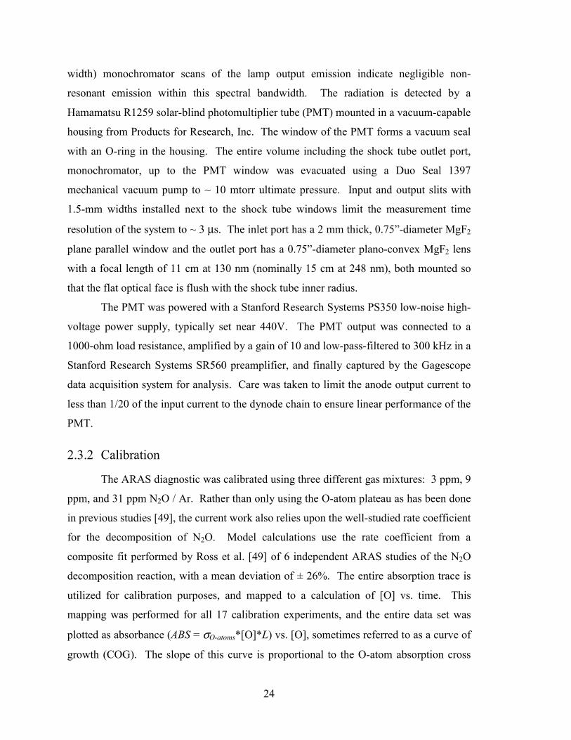
24

width) monochromator scans of the lamp output emission indicate negligible non-

resonant emission within this spectral bandwidth. The radiation is detected by a

Hamamatsu R1259 solar-blind photomultiplier tube (PMT) mounted in a vacuum-capable

housing from Products for Research, Inc. The window of the PMT forms a vacuum seal

with an O-ring in the housing. The entire volume including the shock tube outlet port,

monochromator, up to the PMT window was evacuated using a Duo Seal 1397

mechanical vacuum pump to ~ 10 mtorr ultimate pressure. Input and output slits with

1.5-mm widths installed next to the shock tube windows limit the measurement time

resolution of the system to ~ 3 µs. The inlet port has a 2 mm thick, 0.75”-diameter MgF2

plane parallel window and the outlet port has a 0.75”-diameter plano-convex MgF2 lens

with a focal length of 11 cm at 130 nm (nominally 15 cm at 248 nm), both mounted so

that the flat optical face is flush with the shock tube inner radius.

The PMT was powered with a Stanford Research Systems PS350 low-noise high-

voltage power supply, typically set near 440V. The PMT output was connected to a

1000-ohm load resistance, amplified by a gain of 10 and low-pass-filtered to 300 kHz in a

Stanford Research Systems SR560 preamplifier, and finally captured by the Gagescope

data acquisition system for analysis. Care was taken to limit the anode output current to

less than 1/20 of the input current to the dynode chain to ensure linear performance of the

PMT.

2.3.2 Calibration

The ARAS diagnostic was calibrated using three different gas mixtures: 3 ppm, 9

ppm, and 31 ppm N2O / Ar. Rather than only using the O-atom plateau as has been done

in previous studies [49], the current work also relies upon the well-studied rate coefficient

for the decomposition of N2O. Model calculations use the rate coefficient from a

composite fit performed by Ross et al. [49] of 6 independent ARAS studies of the N2O

decomposition reaction, with a mean deviation of ± 26%. The entire absorption trace is

utilized for calibration purposes, and mapped to a calculation of [O] vs. time. This

mapping was performed for all 17 calibration experiments, and the entire data set was

plotted as absorbance (ABS = σO-atoms*[O]*L) vs. [O], sometimes referred to as a curve of

growth (COG). The slope of this curve is proportional to the O-atom absorption cross

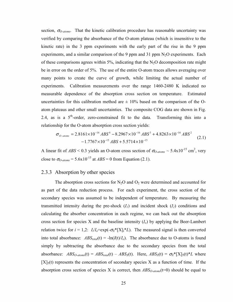
25

section, σO-atoms. That the kinetic calibration procedure has reasonable uncertainty was

verified by comparing the absorbance of the O-atom plateau (which is insensitive to the

kinetic rate) in the 3 ppm experiments with the early part of the rise in the 9 ppm

experiments, and a similar comparison of the 9 ppm and 31 ppm N2O experiments. Each

of these comparisons agrees within 5%, indicating that the N2O decomposition rate might

be in error on the order of 5%. The use of the entire O-atom traces allows averaging over

many points to create the curve of growth, while limiting the actual number of

experiments. Calibration measurements over the range 1460-2480 K indicated no

measurable dependence of the absorption cross section on temperature. Estimated

uncertainties for this calibration method are ± 10% based on the comparison of the O-

atom plateaus and other small uncertainties. The composite COG data are shown in Fig.

2.4, as is a 5th-order, zero-constrained fit to the data. Transforming this into a

relationship for the O-atom absorption cross section yields:

1515

216316416

105714.5107767.1

108263.4102967.8108161.2−−

−−−−

×+×−

×+×−×=

ABSABSABSABSatomsOσ

(2.1)

A linear fit of ABS < 0.3 yields an O-atom cross section of σO-atoms ~ 5.4x10-15 cm2, very

close to σO-atoms = 5.6x10-15 at ABS = 0 from Equation (2.1).

2.3.3 Absorption by other species

The absorption cross sections for N2O and O2 were determined and accounted for

as part of the data reduction process. For each experiment, the cross section of the

secondary species was assumed to be independent of temperature. By measuring the

transmitted intensity during the pre-shock (I1) and incident shock (I2) conditions and

calculating the absorber concentration in each regime, we can back out the absorption

cross section for species X and the baseline intensity (Io) by applying the Beer-Lambert

relation twice for i = 1,2: Ii/Io=exp(-σX*[X]i*L). The measured signal is then converted

into total absorbance: ABStotal(t) = -ln(I(t)/Io). The absorbance due to O-atoms is found

simply by subtracting the absorbance due to the secondary species from the total

absorbance: ABSO-atoms(t) = ABStotal(t) – ABSX(t). Here, ABSX(t) = σX*[X]5(t)*L where

[X]5(t) represents the concentration of secondary species X as a function of time. If the

absorption cross section of species X is correct, then ABSO-atoms(t=0) should be equal to

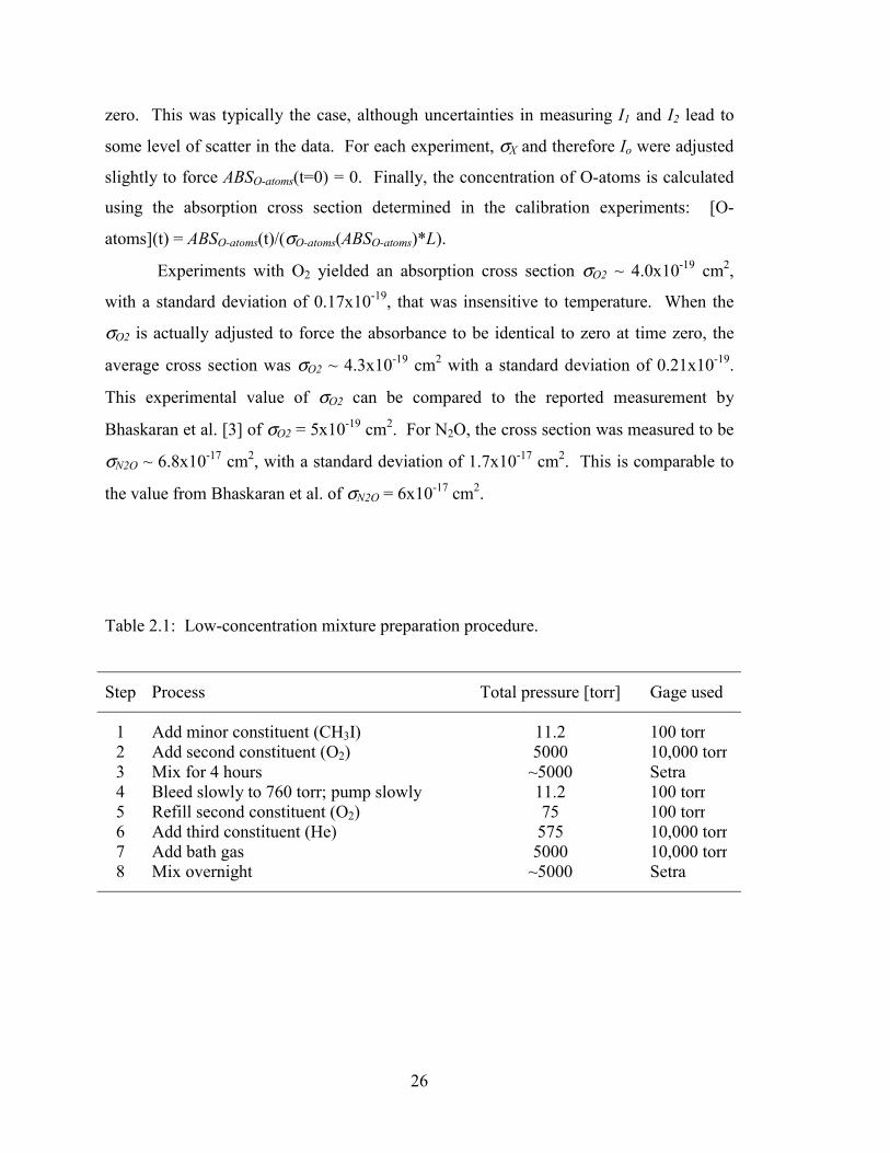
26

zero. This was typically the case, although uncertainties in measuring I1 and I2 lead to

some level of scatter in the data. For each experiment, σX and therefore Io were adjusted

slightly to force ABSO-atoms(t=0) = 0. Finally, the concentration of O-atoms is calculated

using the absorption cross section determined in the calibration experiments: [O-

atoms](t) = ABSO-atoms(t)/(σO-atoms(ABSO-atoms)*L).

Experiments with O2 yielded an absorption cross section σO2 ~ 4.0x10-19 cm2,

with a standard deviation of 0.17x10-19, that was insensitive to temperature. When the

σO2 is actually adjusted to force the absorbance to be identical to zero at time zero, the

average cross section was σO2 ~ 4.3x10-19 cm2 with a standard deviation of 0.21x10-19.

This experimental value of σO2 can be compared to the reported measurement by

Bhaskaran et al. [3] of σO2 = 5x10-19 cm2. For N2O, the cross section was measured to be

σN2O ~ 6.8x10-17 cm2, with a standard deviation of 1.7x10-17 cm2. This is comparable to

the value from Bhaskaran et al. of σN2O = 6x10-17 cm2.

Table 2.1: Low-concentration mixture preparation procedure.

Step Process Total pressure [torr] Gage used

1 Add minor constituent (CH3I) 11.2 100 torr 2 Add second constituent (O2) 5000 10,000 torr3 Mix for 4 hours ~5000 Setra 4 Bleed slowly to 760 torr; pump slowly 11.2 100 torr 5 Refill second constituent (O2) 75 100 torr 6 Add third constituent (He) 575 10,000 torr7 Add bath gas 5000 10,000 torr8 Mix overnight ~5000 Setra

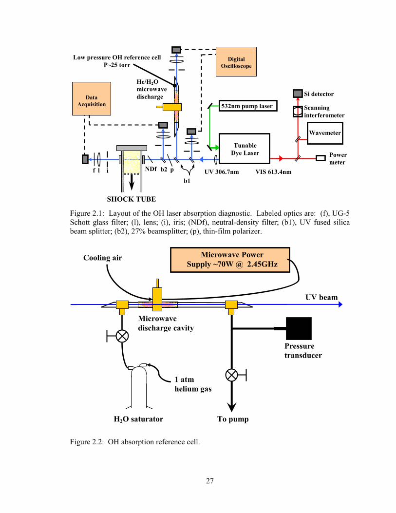
27

Figure 2.1: Layout of the OH laser absorption diagnostic. Labeled optics are: (f), UG-5 Schott glass filter; (l), lens; (i), iris; (NDf), neutral-density filter; (b1), UV fused silica beam splitter; (b2), 27% beamsplitter; (p), thin-film polarizer.

Figure 2.2: OH absorption reference cell.

Powermeter

532nm pump laser

Tunable Dye Laser

Scanning interferometer

Si detector

Wavemeter

He/H2O microwavedischarge

Low pressure OH reference cellP~25 torr

Data Acquisition

SHOCK TUBE

Digital

Oscilloscope

VIS 613.4nm UV 306.7nml f i pb2 NDf

b1

Microwave Power Supply ~70W @ 2.45GHz

To pump

Cooling air

1 atm helium gas

H2O saturator

Pressure transducer

UV beam

Microwave discharge cavity

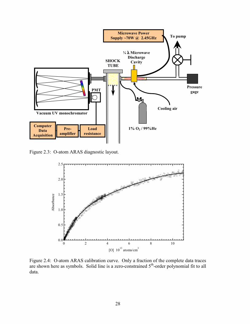
28

Figure 2.3: O-atom ARAS diagnostic layout.

2.5

2.0

1.5

1.0

0.5

0.0

Abs

orba

nce

1086420

[O] 1013 atoms/cm3

Figure 2.4: O-atom ARAS calibration curve. Only a fraction of the complete data traces are shown here as symbols. Solid line is a zero-constrained 5th-order polynomial fit to all data.

SHOCK TUBE

Microwave Power Supply ~70W @ 2.45GHz

Vacuum UV monochromator

PMT

1% O2 / 99%He

Cooling air

¼ λλλλ Microwave Discharge

Cavity

Pressure gage

Computer Data

Acquisition

To pump

Load resistance

Pre- amplifier

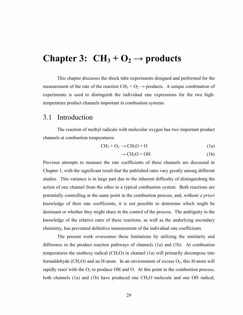
29

Chapter 3: CH3 + O2 → products

This chapter discusses the shock tube experiments designed and performed for the

measurement of the rate of the reaction CH3 + O2 → products. A unique combination of

experiments is used to distinguish the individual rate expressions for the two high-

temperature product channels important in combustion systems.

3.1 Introduction The reaction of methyl radicals with molecular oxygen has two important product

channels at combustion temperatures:

CH3 + O2 → CH3O + O (1a)

→ CH2O + OH (1b)

Previous attempts to measure the rate coefficients of these channels are discussed in

Chapter 1, with the significant result that the published rates vary greatly among different

studies. This variance is in large part due to the inherent difficulty of distinguishing the

action of one channel from the other in a typical combustion system. Both reactions are

potentially controlling at the same point in the combustion process, and, without a priori

knowledge of their rate coefficients, it is not possible to determine which might be

dominant or whether they might share in the control of the process. The ambiguity in the

knowledge of the relative rates of these reactions, as well as the underlying secondary

chemistry, has prevented definitive measurement of the individual rate coefficients.

The present work overcomes these limitations by utilizing the similarity and

difference in the product reaction pathways of channels (1a) and (1b). At combustion

temperatures the methoxy radical (CH3O) in channel (1a) will primarily decompose into

formaldehyde (CH2O) and an H-atom. In an environment of excess O2, this H-atom will

rapidly react with the O2 to produce OH and O. At this point in the combustion process,

both channels (1a) and (1b) have produced one CH2O molecule and one OH radical,

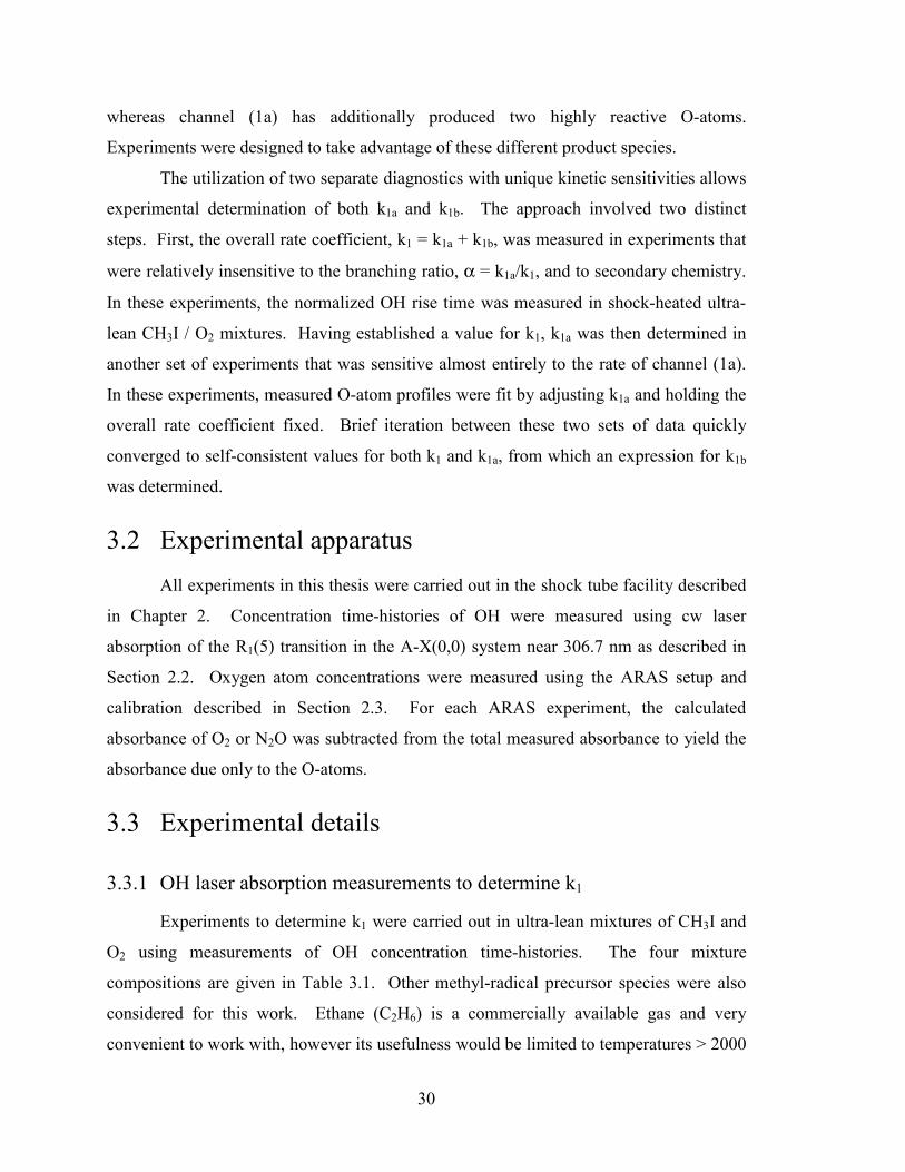
30

whereas channel (1a) has additionally produced two highly reactive O-atoms.

Experiments were designed to take advantage of these different product species.

The utilization of two separate diagnostics with unique kinetic sensitivities allows

experimental determination of both k1a and k1b. The approach involved two distinct

steps. First, the overall rate coefficient, k1 = k1a + k1b, was measured in experiments that

were relatively insensitive to the branching ratio, α = k1a/k1, and to secondary chemistry.

In these experiments, the normalized OH rise time was measured in shock-heated ultra-

lean CH3I / O2 mixtures. Having established a value for k1, k1a was then determined in

another set of experiments that was sensitive almost entirely to the rate of channel (1a).

In these experiments, measured O-atom profiles were fit by adjusting k1a and holding the

overall rate coefficient fixed. Brief iteration between these two sets of data quickly

converged to self-consistent values for both k1 and k1a, from which an expression for k1b

was determined.

3.2 Experimental apparatus All experiments in this thesis were carried out in the shock tube facility described

in Chapter 2. Concentration time-histories of OH were measured using cw laser

absorption of the R1(5) transition in the A-X(0,0) system near 306.7 nm as described in

Section 2.2. Oxygen atom concentrations were measured using the ARAS setup and

calibration described in Section 2.3. For each ARAS experiment, the calculated

absorbance of O2 or N2O was subtracted from the total measured absorbance to yield the

absorbance due only to the O-atoms.

3.3 Experimental details

3.3.1 OH laser absorption measurements to determine k1

Experiments to determine k1 were carried out in ultra-lean mixtures of CH3I and

O2 using measurements of OH concentration time-histories. The four mixture

compositions are given in Table 3.1. Other methyl-radical precursor species were also

considered for this work. Ethane (C2H6) is a commercially available gas and very

convenient to work with, however its usefulness would be limited to temperatures > 2000

31

K due to its slow decomposition rate. Azomethane ((CH3)2N2) decomposes easily at low

temperatures, but caution must be used as it may decompose and react behind the

incident shock wave at higher temperatures. It is also inconvenient, in that azomethane

cannot be purchased and must be synthesized in the laboratory. CH3I was chosen for the

entire set of experiments because it is easy to work with and its decomposition is well

characterized at the conditions of interest for this study.

Mixtures were optimized to achieve good signal/noise, short OH rise times (< 100

µs) to minimize effects of boundary layer-induced changes in the reflected shock

temperature and pressure, optimum sensitivity to and isolation of the overall reaction rate

coefficient, and minimum sensitivity to the branching ratio as well as secondary

reactions. Effects of O2 vibrational relaxation were minimized by the addition of helium.

Sensitivity analysis indicates that the initial rate of increase of the OH concentration is

sensitive primarily to reactions (1a) and (1b). Specifically, the normalized rise time from

10-50% of the peak OH concentration, ∆t(10-50%), yields high sensitivity to the overall

rate coefficient k1 and low sensitivity to the branching ratio α and secondary reactions.

Therefore, the overall rate coefficient could be determined independent of an a priori

assumption of dominance by either channel. Use of the 10-50% rise time gives almost

identical sensitivities as does the half rise time, τ1/2, used in other recent investigations

[12,24], with the added benefit that it is insensitive to small errors in the determination of

time zero. Although several secondary reactions become important at the OH peak,

normalizing the rise time by the peak mole fraction deemphasizes this sensitivity and

allows reaction (1) to be well isolated.

An example brute-force sensitivity analysis calculated using the GRI-Mech 3.0

mechanism [37], updated with the new values for k1a and k1b and the heat of formation of

OH given in Chapter 4, is shown in Fig. 3.1. Sensitivity of ∆t(10-50%) for each reaction

i was calculated by individually perturbing rate coefficients and using the following

equation:

( ) ( )( )( ) ( )i

i

ii

iii kt

kkk

ktktS∆−

∆−∆= *5.02

5.02 (3.1)

For the sensitivity to α, ki was replaced by α and the factors 2 and 0.5 were replaced by

the multiplicative factors which made α = 1 or 0. As can be seen in Fig. 3.1, sensitivity

32

of ∆t(10-50%) is dominated by the overall reaction rate k1, and the sensitivity to the

branching ratio α is approximately 1/10 the k1 sensitivity. The secondary reaction

uncertainties and their effect on the final reduced reaction rate coefficient are taken into

account in the uncertainty analysis.

3.3.2 O-atom ARAS measurements to determine k1a

To determine k1a, experiments were performed using the mixture compositions

given in Table 3.2. The experimental mixtures and conditions were chosen to optimize

the sensitivity to reaction (1a), deemphasize reaction (1b) and other secondary chemistry,

achieve good signal/noise (maximize O-atom absorption and minimize O2 absorption),

and reduce effects of vibrational relaxation of O2. An example sensitivity calculation

performed with the SENKIN program [50] is shown in Fig. 3.2. The O-atom

concentration is strongly sensitive to the O-atom product channel, (1a), and only weakly

sensitive to the OH product channel (1b) and secondary reactions.

The present O-atom experiments differ slightly from those in Michael et al. [16].

Whereas they used ~ 1.6-2.5 ppm CH3I / 6-11% O2, the present mixtures use lower O2

and higher CH3I concentrations. While this mixture choice gives slightly poorer kinetic

isolation, there are several reasons for this selection of reaction mixtures. First, the larger

diameter of our shock tube increases the absorption path length of all absorbers, including

O2. Because molecular oxygen has a very large absorption cross section at 130 nm, even

with only 1.5% O2 up to 38% of the lamp emission is absorbed by the O2. Higher O2

concentrations therefore decrease signal levels and thus the signal/noise ratio. Second,

high O2 concentrations result in increased vibrational relaxation effects on the

temperature and pressure and degrade shock tube performance. The goal was to

minimize both the temperature and pressure gradients as the O2 relaxed vibrationally, as

well as the relaxation time itself.

In the present study, by keeping O2 concentrations low and adding 10% helium

(He), these relaxation issues were minimized, and good confidence was maintained in the

calculated temperature and pressure. The addition of helium reduces the vibrational

relaxation time of a mixture of 1.5% O2 / Ar at 1800 K, 1.4 atm from 32 µs to 4 µs,

calculated for the mixture using coefficients from Millikan [51]. The addition of helium

33

also results in higher confidence in the temperature and pressure calculated from the

normal shock equations, in that the post-incident shock gases are fully relaxed by the

time the reflected shock returns, and the post-reflected shock gases quickly equilibrate

before significant chemistry takes place. In addition, potential effects that vibrational

non-equilibrium may have on the chemistry itself are avoided.

Higher CH3I concentrations than in Michael et al. [16] were used due to the lower

absorption cross section of our lamp configuration and also to minimize the relative

effects of residual impurities in the gas handling system (see the next section).

3.3.3 Impurity issues

Ultra-lean, ultra-low concentration gas mixtures were required in this work in

order to achieve high chemical isolation of and sensitivity to the title reactions. This

means creating mixtures with ppm-level hydrocarbon concentrations and %-level oxygen

concentrations. The obvious concerns with this situation are 1) the ability to make well-

controlled accurate mixtures and 2) the potential effects of residual impurities in the gas

handling system and shock tube. The mixture-making process was discussed in Section

2.1.3. The amount of residual impurities, their reduction and control, and their effect on

the chemical kinetic measurements are discussed here.

Prior to the work on CH3+O2, experiments had been performed in this shock tube

using a variety of large hydrocarbon fuels. In addition, hydrocarbon solvents,

specifically acetone and methanol, are typically used to clean the shock tube walls.

Because of the concern of hydrocarbon impurities, experiments for this work were

initially performed with a mixture of 10% O2 / Ar (no added hydrocarbon). In these

experiments, a finite level of OH was measured using the OH laser absorption diagnostic.

After a few more shocks, this level decreased somewhat as residual cleaning solvents

were removed from the shock tube walls by the action of the shock waves and vacuum

system; however, the level seemed to bottom out near 10 ppm OH at shock temperatures

near 1800 K. In an effort to try to characterize the OH behavior and its source, model

calculations with ~ 8 ppm CH3 added to the mixture gave a reasonable match to the

measured temporal behavior and plateau OH concentrations. This level of effective

34

“impurity” was clearly unacceptable for this work, and a plan was developed to find and

fix the impurity source.

Impurities can only come from a limited number of sources in a shock tube

system: the gas bottles, surfaces and semi-trapped volumes in the gas handling system

(valves, piping, mixing tank, and connections of these components), the vacuum system

(primarily backstreaming pump oil), and crevices and surfaces in the shock tube itself.

To track down the general area of the impurity source, experiments were performed with

pure O2 while different parts of the system were bypassed. First, O2 was flowed into the

shock tube through the mixing manifold but without using the mixing tank. This resulted

in a drop of the measured OH from 10.5 to 6.4 ppm. Next, the O2 was connected directly

to a port in the middle of the shock tube (bypassing the manifold), and the level dropped

to near 1 ppm at 1700 K. When the oxygen cylinder was moved so that the gas flowed

from the endwall back towards the diaphragm, no change was observed. This removed

the possibility that the fill gases were sweeping residual impurity vapors from the whole

tube length down to the endwall and amplifying their effect. This set of experiments

quickly identified the mixing manifold and mixing tank as the most likely major sources

of impurities. Supporting this conclusion was the observation that impurities seemed to

increase over a few days’ time as a particular mixture remained in the mixing tank.

The gas mixing system was originally evacuated with only a two-stage direct-

drive mechanical pump. This pump had an ultimate vacuum no lower than 1 mtorr

(1x10-3 torr) at the pump and typically much higher vacuum at the farthest reaches of the

system. This was now deemed to be unsatisfactory, and a new vacuum system was

designed incorporating a turbomolecular pump. The new setup is described in Section

2.1.2. An effort was made to keep all vacuum lines as large in diameter and short in

length as possible to improve system pumping speed, and the previous 100”-long ¼”-

diameter fill line from the mixing manifold to the shock tube was replaced by a 40”-long

3/8”-diameter line. New vented stem inserts were installed in all of the bellows-sealed

valves to reduce the possibility of slow-leakage of trapped gasses within the valve

mechanism.

Vacuum performance of the rebuilt gas mixing system was greatly improved, with

ultimate vacuum pressures of ~ 1 µtorr. New experiments with a 100% O2 “mixture” in

35

the tank produced OH plateaus of ~ 2 ppm near 1750 K. A 10% O2 / Ar mixture (similar

to potential chemical kinetics experiments) yielded 0.8 ppm and 2 ppm OH near 1850 K

and 2150 K, respectively. Mixtures with 0.32 ppm CH3 and 0.8 ppm CH3 “impurity”

were sufficient to model the OH production. These impurity levels were now at or below

previous experiments where the mixing system was bypassed – indicating that the major

issues in the mixing system had been rectified.

Attempts were made to further reduce the impurity level. All shock tube ports

were removed, cleaned, and replaced with the absolute minimum amount of vacuum

grease required to maintain vacuum integrity. Both the shock tube and mixing tank were

baked at high vacuum in an attempt to drive adsorbed impurity species from the walls

and crevices of these vessels. These actions yielded negligible improvement, and in fact

the impurity was typically temporarily worse until the baked-off species had been

sufficiently eliminated from the system and everything settled back down to levels

achieved before baking. Aluminum foil diaphragms 0.001” and 0.003” thickness were

tried in place of the polycarbonate diaphragms, as the plastic has been known to shed

measurable levels of H-atoms during the diaphragm burst process. This, again, produced

little change in the effective impurity. Finally, gases with higher stated purity were used,

including 99.9999% purity Ar (in place of the original 99.999%) and 99.999% pure O2

(in place of the original 99.993%). Neither of these had a significant effect.

While the experimentally measured effects of the “impurities” were not

completely negligible, they were significantly smaller and well-characterized with

discrete but small levels of CH3 (or H-atoms at the highest temperatures) added to the

mixture. With a realistic assessment of our resources, the decision was made to accept

the current performance of the system, characterize the impurity, and include it in the

analysis for all future kinetics experiments. The issue would be revisited if it became a

limiting uncertainty in this work.

Impurity effects were characterized independently for each gas mixture, using

experiments with no added CH3I. Both in OH and O-atom experiments, measurable

radical concentrations were modeled with CH3 radicals added to the nominal O2 / Ar

mixture. At the highest temperatures of this study (> 2400 K), the impurity behavior was

modeled more closely with H-atoms as the surrogate (or real) impurity species. The

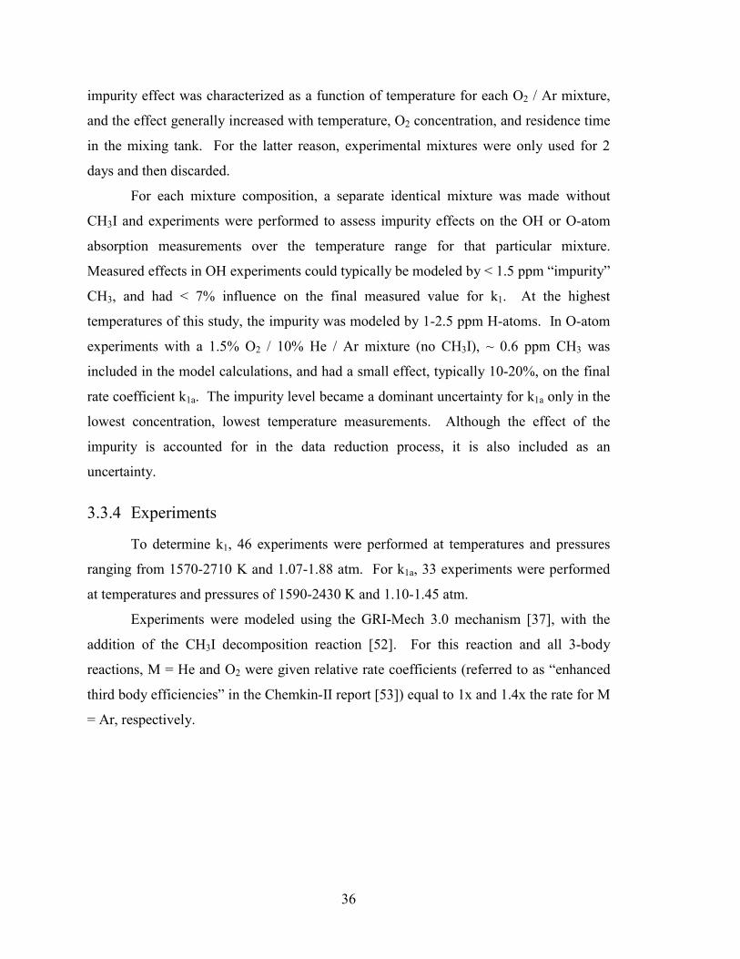
36

impurity effect was characterized as a function of temperature for each O2 / Ar mixture,

and the effect generally increased with temperature, O2 concentration, and residence time

in the mixing tank. For the latter reason, experimental mixtures were only used for 2

days and then discarded.

For each mixture composition, a separate identical mixture was made without

CH3I and experiments were performed to assess impurity effects on the OH or O-atom

absorption measurements over the temperature range for that particular mixture.

Measured effects in OH experiments could typically be modeled by < 1.5 ppm “impurity”

CH3, and had < 7% influence on the final measured value for k1. At the highest

temperatures of this study, the impurity was modeled by 1-2.5 ppm H-atoms. In O-atom

experiments with a 1.5% O2 / 10% He / Ar mixture (no CH3I), ~ 0.6 ppm CH3 was

included in the model calculations, and had a small effect, typically 10-20%, on the final

rate coefficient k1a. The impurity level became a dominant uncertainty for k1a only in the

lowest concentration, lowest temperature measurements. Although the effect of the

impurity is accounted for in the data reduction process, it is also included as an

uncertainty.

3.3.4 Experiments

To determine k1, 46 experiments were performed at temperatures and pressures

ranging from 1570-2710 K and 1.07-1.88 atm. For k1a, 33 experiments were performed

at temperatures and pressures of 1590-2430 K and 1.10-1.45 atm.

Experiments were modeled using the GRI-Mech 3.0 mechanism [37], with the

addition of the CH3I decomposition reaction [52]. For this reaction and all 3-body

reactions, M = He and O2 were given relative rate coefficients (referred to as “enhanced

third body efficiencies” in the Chemkin-II report [53]) equal to 1x and 1.4x the rate for M

= Ar, respectively.

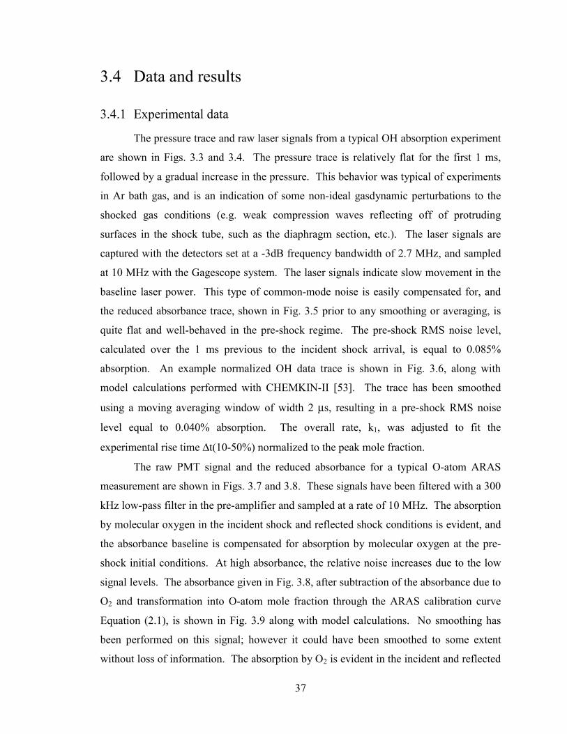
37

3.4 Data and results

3.4.1 Experimental data

The pressure trace and raw laser signals from a typical OH absorption experiment

are shown in Figs. 3.3 and 3.4. The pressure trace is relatively flat for the first 1 ms,

followed by a gradual increase in the pressure. This behavior was typical of experiments

in Ar bath gas, and is an indication of some non-ideal gasdynamic perturbations to the

shocked gas conditions (e.g. weak compression waves reflecting off of protruding

surfaces in the shock tube, such as the diaphragm section, etc.). The laser signals are

captured with the detectors set at a -3dB frequency bandwidth of 2.7 MHz, and sampled

at 10 MHz with the Gagescope system. The laser signals indicate slow movement in the

baseline laser power. This type of common-mode noise is easily compensated for, and

the reduced absorbance trace, shown in Fig. 3.5 prior to any smoothing or averaging, is

quite flat and well-behaved in the pre-shock regime. The pre-shock RMS noise level,

calculated over the 1 ms previous to the incident shock arrival, is equal to 0.085%

absorption. An example normalized OH data trace is shown in Fig. 3.6, along with

model calculations performed with CHEMKIN-II [53]. The trace has been smoothed

using a moving averaging window of width 2 µs, resulting in a pre-shock RMS noise

level equal to 0.040% absorption. The overall rate, k1, was adjusted to fit the

experimental rise time ∆t(10-50%) normalized to the peak mole fraction.

The raw PMT signal and the reduced absorbance for a typical O-atom ARAS

measurement are shown in Figs. 3.7 and 3.8. These signals have been filtered with a 300

kHz low-pass filter in the pre-amplifier and sampled at a rate of 10 MHz. The absorption

by molecular oxygen in the incident shock and reflected shock conditions is evident, and

the absorbance baseline is compensated for absorption by molecular oxygen at the pre-

shock initial conditions. At high absorbance, the relative noise increases due to the low

signal levels. The absorbance given in Fig. 3.8, after subtraction of the absorbance due to

O2 and transformation into O-atom mole fraction through the ARAS calibration curve

Equation (2.1), is shown in Fig. 3.9 along with model calculations. No smoothing has

been performed on this signal; however it could have been smoothed to some extent

without loss of information. The absorption by O2 is evident in the incident and reflected

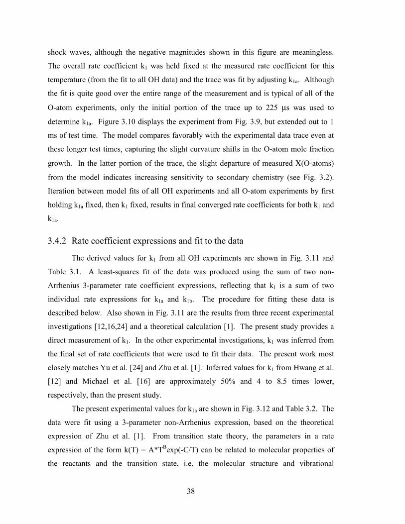
38

shock waves, although the negative magnitudes shown in this figure are meaningless.

The overall rate coefficient k1 was held fixed at the measured rate coefficient for this

temperature (from the fit to all OH data) and the trace was fit by adjusting k1a. Although

the fit is quite good over the entire range of the measurement and is typical of all of the

O-atom experiments, only the initial portion of the trace up to 225 µs was used to

determine k1a. Figure 3.10 displays the experiment from Fig. 3.9, but extended out to 1

ms of test time. The model compares favorably with the experimental data trace even at

these longer test times, capturing the slight curvature shifts in the O-atom mole fraction

growth. In the latter portion of the trace, the slight departure of measured Χ(O-atoms)

from the model indicates increasing sensitivity to secondary chemistry (see Fig. 3.2).

Iteration between model fits of all OH experiments and all O-atom experiments by first

holding k1a fixed, then k1 fixed, results in final converged rate coefficients for both k1 and

k1a.

3.4.2 Rate coefficient expressions and fit to the data

The derived values for k1 from all OH experiments are shown in Fig. 3.11 and

Table 3.1. A least-squares fit of the data was produced using the sum of two non-

Arrhenius 3-parameter rate coefficient expressions, reflecting that k1 is a sum of two

individual rate expressions for k1a and k1b. The procedure for fitting these data is

described below. Also shown in Fig. 3.11 are the results from three recent experimental

investigations [12,16,24] and a theoretical calculation [1]. The present study provides a

direct measurement of k1. In the other experimental investigations, k1 was inferred from

the final set of rate coefficients that were used to fit their data. The present work most

closely matches Yu et al. [24] and Zhu et al. [1]. Inferred values for k1 from Hwang et al.

[12] and Michael et al. [16] are approximately 50% and 4 to 8.5 times lower,

respectively, than the present study.

The present experimental values for k1a are shown in Fig. 3.12 and Table 3.2. The

data were fit using a 3-parameter non-Arrhenius expression, based on the theoretical

expression of Zhu et al. [1]. From transition state theory, the parameters in a rate

expression of the form k(T) = A*TBexp(-C/T) can be related to molecular properties of

the reactants and the transition state, i.e. the molecular structure and vibrational

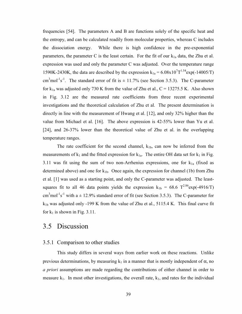
39

frequencies [54]. The parameters A and B are functions solely of the specific heat and

the entropy, and can be calculated readily from molecular properties, whereas C includes

the dissociation energy. While there is high confidence in the pre-exponential

parameters, the parameter C is the least certain. For the fit of our k1a data, the Zhu et al.

expression was used and only the parameter C was adjusted. Over the temperature range

1590K-2430K, the data are described by the expression k1a = 6.08x107T1.54exp(-14005/T)

cm3mol-1s-1. The standard error of fit is ± 11.7% (see Section 3.5.3). The C-parameter

for k1a was adjusted only 730 K from the value of Zhu et al., C = 13275.5 K. Also shown

in Fig. 3.12 are the measured rate coefficients from three recent experimental

investigations and the theoretical calculation of Zhu et al. The present determination is

directly in line with the measurement of Hwang et al. [12], and only 32% higher than the

value from Michael et al. [16]. The above expression is 42-55% lower than Yu et al.

[24], and 26-37% lower than the theoretical value of Zhu et al. in the overlapping

temperature ranges.

The rate coefficient for the second channel, k1b, can now be inferred from the

measurements of k1 and the fitted expression for k1a. The entire OH data set for k1 in Fig.

3.11 was fit using the sum of two non-Arrhenius expressions, one for k1a (fixed as

determined above) and one for k1b. Once again, the expression for channel (1b) from Zhu

et al. [1] was used as a starting point, and only the C-parameter was adjusted. The least-

squares fit to all 46 data points yields the expression k1b = 68.6 T2.86exp(-4916/T)

cm3mol-1s-1 with a ± 12.9% standard error of fit (see Section 3.5.3). The C-parameter for

k1b was adjusted only -199 K from the value of Zhu et al., 5115.4 K. This final curve fit

for k1 is shown in Fig. 3.11.

3.5 Discussion

3.5.1 Comparison to other studies

This study differs in several ways from earlier work on these reactions. Unlike

previous determinations, by measuring k1 in a manner that is mostly independent of α, no

a priori assumptions are made regarding the contributions of either channel in order to

measure k1. In most other investigations, the overall rate, k1, and rates for the individual

40

product channels often depended, sometimes strongly, on the accuracy of the assumed

rate coefficient for one of the channels. In addition, the use of very low CH3I / O2 ratios

has enabled sensitive measurement of the overall reaction rate without significant

sensitivity to secondary chemistry.

While the present expression for k1a is in agreement with Michael et al. [16] and

Hwang et al. [12], the measurement of the overall rate k1 and the inference of k1b

represent a significant departure from these two studies. The present experimental rate

expression for k1b is 2-3x higher than the rate used by Hwang et al. in the modeling of

their data, and the dominance of channel (1b) in our study clearly disagrees with the

conclusion of Michael et al. that this channel is unimportant.

A recent literature debate [55-57] centers on boundary layer-induced temperature

effects in shock tube experiments, and the correction that has been systematically applied

by some investigators [12,16] and not by others [24]. In CH4 ignition experiments

identical to Yu et al. [24], Hwang et al. [12] measure comparable characteristic OH

induction times yet their published rate for k1a is a factor of 2.5x lower than Yu et al. In

that study, the authors make the observation that the average applied temperature

correction of 24 K, based on boundary layer interaction with the reflected shock wave, is

the primary cause for the difference in their final rate coefficient for k1a compared to Yu

et al. They further suggest that if the appropriate correction were applied to the

experiments of [24], excellent agreement between the two studies is obtained. In the

ensuing literature debate, the justification and reliability of a standard boundary layer-

induced temperature correction was both refuted [55] and supported [56,57].

The very nature of the high sensitivity to temperature of the CH4 ignition time

studies (+24 K → 2.5x uncertainty in k1a) calls into question their desirability as sensitive

measurement of the title reactions. As pointed out by Michael et al. [56], experiments in

ultra-low concentration CH3I mixtures are much less sensitive to slight temperature

changes than are CH4 ignition experiments. Therefore, the use or non-use of boundary

layer corrections had little effect on their final reduced chemistry. The same argument

applies to the present study. In addition, the larger diameter of our shock tube (14.13 cm

compared to 8.26 cm [24], 9.74 cm [16], and a rolled-square shock tube with diameter

6.35 cm [12]) results in smaller temperature effects due to the growth of the boundary

41

layer, as the perturbation is a surface-to-volume ratio effect [58,59]. Finally, all kinetic

measurements in the present study were performed at experimental test times well under

200-300 µs, and thus any potential gas dynamic changes in temperature and pressure due

to boundary layer growth are only in their early stages of development. For these

reasons, systematic temperature corrections were not applied in this study and are

believed to be of little consequence to the final rate coefficient expressions.

3.5.2 Constrained vs. unconstrained rate expression fits

The present fits to the experimental data, constrained by the pre-exponential

coefficients of Zhu et al. [1], can be compared to similar curve fits without any

constraints on the parameters. Performing an unconstrained 3-parameter fit of the k1a

data in Fig. 3.12 results in a standard error of fit similar to that for the constrained fit. An

unconstrained 6-parameter fit of the k1 data in Fig. 3.11 (fixing the expression for k1a

from the unconstrained fit) results in standard error of fit of 8.2%, compared to 12.9% in

the final constrained fit using the Zhu et al. pre-exponential coefficients. The slight

deviation of the k1 fit from the data at high temperatures in Fig. 3.11 is due to the

simultaneous constraint of the k1a expression determined from the O-atom experiments

and the Zhu et al. pre-exponential coefficients for k1b. The differences in the fitting

parameters between the unconstrained and constrained fits are small, as evidenced by the

almost imperceptible changes in the quality of the fits, and are well within the uncertainty

bounds of the present measurements. Therefore, the pre-exponential coefficients from

the theoretically-determined expressions of Zhu et al. have been retained, and the data is

fit by adjusting only the C-parameter. Basing the fits on the theoretical calculations of

Zhu et al. gives higher confidence in extrapolating the present rate expressions outside of

the present experimental temperature range. The change in the C-parameter for k1a

represents an adjustment in the heat of formation of CH3O of ≈ +6.1 kJ/mol. This

modification is on the order of previous uncertainties in the heat of formation [60]. The

C-parameter for k1b changed slightly from the value of Zhu et al., representing an

adjustment in the barrier height of ≈ -1.7 kJ/mol.

42

3.5.3 Uncertainty analysis

The confidence limits in the new rate expressions are evaluated from the scatter in

the experimental measurements and an assessment of systematic uncertainties. The

scatter in the data is characterized by the standard error of fit, Syx, a measure of the

precision with which a function y(x) describes the behavior of the set [61]. Because the

rate coefficient data span more than an order of magnitude, the deviation of an individual

data point from the curve fit is considered as a percent deviation rather than an absolute

number. The standard error of fit is calculated using Equation (3.2):

ν

∑=

−

=

N

i ci

cii

yx

yyy

S 1

2

(3.2)

In this equation, N is the number of data points; yi and yci are the measured and curve fit

values (rate coefficients) at a given value of the dependent variable (temperature); and ν

is the degrees of freedom of the fit and is equal to N – (m+1), where m is the order of the

polynomial used to fit the data. For our fit we have one free variable, similar to a 0th

order polynomial, so m = 0. As previously mentioned, the curve fits of the data in Figs.

3.11 and 3.12 yield standard errors of fit of 12.9% and 11.7% for k1 and k1a, respectively.

Detailed assessments of the possible systematic errors for k1 and k1a were

performed for individual experiments at the high- and low-temperature limits of this

study. These points typically represent the expected maximum-uncertainty conditions, as

anticipated error sources limited the expansion of the experimental set to a wider range of

temperatures. The error sources considered for this analysis are shown in Table 3.3.

Potential errors are propagated through to their effect on k1 or k1a through the technique

of sequential perturbation [61]. In this technique, each independent variable’s

uncertainty limits are individually applied to the data reduction process or chemical

kinetic model (or both, in the case of temperature and pressure), and the fit parameter (k1

or k1a) is adjusted to refit the experiment in view of the perturbed conditions. The

adjustment required in the fit parameter is therefore the uncertainty in k1 or k1a from that

perturbation of the independent variable. The absolute uncertainty contributions in the

positive and negative direction for each variable are averaged to give the approximate

total uncertainty contribution from that variable. Shown in Table 3.3 is an example

43

analysis for a k1a experiment at 2428 K. The individual contributions are combined using

the root-sum-squares method, a calculation which is valid for uncorrelated errors which

have all been estimated to similar probabilities (e.g. 95% probability that the true value

falls within the ± error limits). For the specific example in Table 3.3, the total estimated

uncertainty in k1a is ± 35%.

In Table 3.3, uncertainty limits in important secondary rate coefficients have been

assessed based on a recent literature review and evaluation [62], the most current and

accepted study of a particular reaction, and/or a comparison of the GRI-Mech 3.0 rate to

the currently accepted rate coefficient. The reactions were each considered individually

in the analysis.

An alternative method for estimating the uncertainties due to secondary reaction

rate coefficients is to update all relevant reaction rate coefficients at once and refit the

data using the revised mechanism. The base mechanism used in this work, GRI-Mech

3.0, is a set of reactions, rate coefficient expressions, and thermodynamic data based on a

particular starting mechanism and modified through a constrained optimization process to

fit a specific set of experimental targets [37]. The most recent optimization round was

finished in 1998, and therefore does not consider new reaction rate data, thermochemical

data, or experimental targets which have been published during the past six years. The

proper method for updating the GRI-Mech mechanism is through another round of

optimization, including a newly evaluated starting mechanism and potentially an

expanded and updated set of experimental targets. This is a very time-intensive process,

however, and beyond the scope of this thesis. Rather, a revised mechanism was created

simply by updating rate coefficients for the secondary reactions important to this work.

To this end, an extensive literature review was performed for the most sensitive

secondary reactions (based on sensitivity analyses performed in Sections 3.3.1 and 3.3.2),

and out of this set 13 reactions were chosen to be revised. Information regarding the

updated reactions is given in Table 3.4. For most reactions the recent review and

evaluation by Baulch et al. [62] was accepted, except for the pressure-dependent CH2O

decomposition reaction rates which were taken from Friedrichs et al. [63]. Also, while

the rate for CH3 decomposition from [62] was accepted here, their evaluation did not

consider the theoretical work on which the rate in [37] is based and does not include

44

pressure dependence. Changing this particular pair of rate coefficients appears to have a

strong effect, so the new mechanism was applied both with and without a revision in the

rate for CH3 decomposition.

Evaluation of 5 experiments using the updated mechanism did not make a

significant difference in the resulting rate coefficients, as shown in Table 3.5. While this

exercise is one way to estimate about how differently an updated mechanism might

behave, it is not a proper assessment of uncertainties for several reasons. First, it assumes

that a correlated “uncertainty” is applied when making the unidirectional adjustment in

all of the reaction rates to their new values. While new studies of these rates may, in fact,

be closely connected to one another, the entire set of revised rates is not necessarily

correlated. The new rates come from many different sources, some of which will be

more accurate than others and more or less consistent with other experimental work.

Second, this assessment does not take into account the true uncertainty limits applicable

to each of the updated rate coefficients. Finally, GRI-Mech is a mechanism derived

through optimization and is constrained to fit a large set of experimental data targets.

Simply updating individual reaction rates to create a new mechanism ignores the desired

result that the mechanism should best-fit a global set of data. For these reasons, the

treatment of individual reaction uncertainties, as exemplified in Table 3.3, is accepted as

the true contribution of secondary chemistry to the total uncertainties in k1 and k1a.

For the temperature range 1600 K to 2400 K, a conservative estimate of the

uncertainty in k1 is, on average, ± 22%, with little variation in this estimate at the lowest

and highest temperatures. Similar analysis for k1a yields ± 33%. Systematic propagation

of these uncertainties to k1b gives ± 27% at 1600 K and ± 41% at 2400 K, although this is

considered to be somewhat conservative given the scatter in the experimental data. At

the lowest temperatures, the uncertainty estimate is dominated by the reactions of

formaldehyde with O-atoms and OH+HO2↔O2+H2O, impurity effects, and calibration of

the ARAS system. At higher temperatures, uncertainty in reflected shock temperature

and pressure and the ARAS calibration are dominant.

45

3.5.4 Secondary chemistry and OH peak sensitivity

The rate measurements of k1 in this work are relatively insensitive to secondary

chemistry, as discussed in the previous section. This chemical isolation is due, in part, to

the normalization of the traces to the peak OH mole fraction. The normalization process

sensitizes the rise time to the reactions of interest and deemphasizes the secondary

reactions which control the peak OH mole fraction. However, the OH measurements in

this study are, in fact, quantitative, and the comparison of the measured and modeled OH

concentration time-histories may be able to reveal something about the most important

secondary reactions. Several reactions have high sensitivities at the OH peak, with

varying dependence on temperature, and together they control the peak OH mole fraction

and the subsequent decay towards equilibrium.

Figure 3.13 depicts the deviation of the measured OH peak from the model

calculations, expressed as a percentage of the modeled OH peak. The deviation ranges

from -10% to +25%, and a clear non-monotonic temperature dependence is evident over

five different reaction mixtures (including a 10 ppm CH3I / 10% O2 mixture not used in

the k1 determination). Sensitivity analyses were performed for the various mixtures over

their respective ranges of shock tube conditions; the composite analysis in Fig. 3.14

displays the temperature-dependent peak OH sensitivity for the most important secondary

reactions. As is evident in Fig. 3.14, multiple reactions have coincident, high sensitivities

at the OH concentration peak. Many of these reactions also suffer from large

uncertainties at these temperatures.

The information presented in Figs. 3.13 and 3.14 merits a closer examination in

order to determine which reactions are most likely causing errors in the OH peak

concentration. Some reactions can be immediately deemed unlikely culprits due to the

temperature-dependence of their sensitivities, the magnitude or direction of their

uncertainties, or both. The reaction 2OH→O+H2O has an estimated uncertainty of ±25%

[62], so although it displays the highest sensitivity in Fig. 3.14, it is unlikely that it is

producing the size of errors plotted in Fig. 3.13. In addition, the highest sensitivities for

this reaction are found above 1800 K where the OH peak error is decreasing towards

zero. The two CH2O decomposition channels also become sensitive only above 1900 K,

where the OH peak error is small. Thus their uncertainties, while larger than those for

46

2OH→O+H2O, will not compensate for the highest OH peak errors located between 1650

K and 2050 K. The rate coefficients for the pair of HCO reactions, HCO+M→H+CO+M

and HCO+O2→HO2+CO, are expected to change from the current GRI-Mech 3.0

expressions, but in equal proportions. The HCO decomposition reaction has been

reported to be a factor of 2 slower than the GRI-Mech 3.0 rate [62,64], and the rate

coefficient of the reaction HCO+O2→HO2+CO was also recommended to be a factor of 2

slower than the value used in GRI-Mech 3.0 [62]. Thus, updating these two reaction

rates together will have little net effect.

The reaction H+O2+Ar→HO2+Ar has been recently measured by Bates et al. [65],

and its new rate expression is 50% of the GRI-Mech 3.0 rate expression. Updating this

reaction, therefore, will make the OH peak error somewhat worse. On the other hand, the

reaction OH+CH2O→HCO+H2O has recently been measured in our laboratory [66], and

the new measurements confirm the evaluation by Baulch et al. [62] that the rate should be

lowered by 50% from the GRI-Mech 3.0 value. This change will decrease the OH peak

deviation.

The three remaining reactions in Fig. 3.14 are the most probable cause of the OH

peak deviations shown in Fig. 3.13. This suggestion is due, in part, to their large

uncertainties but especially because the temperature-dependence of their sensitivities

closely matches the temperature-dependence of the OH peak deviation. The reaction

OH+HO2→O2+H2O has large uncertainties stemming from limited high-temperature

measurements and complex temperature dependence. At low temperatures, the reaction

rate decreases with temperature, but this appears to change dramatically near 1250K to

strong positive temperature dependence. Hippler et al. [67] observed this swing in

temperature dependence, and while they do not provide an uncertainty for their

measurements, the evaluation of Baulch et al. [62] suggests a factor of 3 uncertainty at

these high temperatures. The rate of the reaction O+CH2O→OH+HCO is based on a fit

of the relatively well-established low-temperature data with one or more of the sparse

high temperature data points – most of which come from flame or shock tube

measurements fit using some type of chemical mechanism. There appears to be a lack of

direct measurements; nevertheless, Baulch et al. [62] assign an uncertainty to this

reaction of only a factor of 2. Finally, the reaction CH2O+O2→HO2+HCO has very

47

limited data of questionable reliability at the shock tube conditions of the present study.

The existing shock tube measurements [16,68] indicate a higher activation energy than

the limited low temperature measurements [69] and theoretical calculations [16,70]

support. The evaluation of Baulch et al. [62] estimates the uncertainty to be a factor of 2

at 600K rising to a factor of 3 at 2500K.

These three reactions, along with some smaller potential contributions from the

other reactions in Fig. 3.14, are most likely responsible for the OH peak deviation

displayed in Fig. 3.13. However, their contributions as a function of temperature (i.e.,

their sensitivities multiplied by their errors) will not necessarily follow the same

temperature dependence shown in Fig. 3.14, and several reactions will need to be

adjusted.

Trial fits were performed by adjusting a specific secondary reaction or set of

reactions to fit the OH peak, while readjusting k1 to retain the fit to the normalized OH

rise time. In general, these adjustments to fit the peak had less than ± 15% effect on the

measurement of k1, but a consistent solution to the peak mismatch problem over a range

of temperatures and mixtures could not be simply determined. To resolve the true

adjustments required for the correct reactions, improved direct determinations for the

rates of these secondary reactions, an optimization scheme, or both, could be undertaken.

Potential directions for this work are discussed in Section 5.3.

3.6 Conclusions The present work provides a direct measurement of the high-temperature channels

of the reaction of CH3 and O2. Through choice of experimental conditions and use of

dilute reactant mixtures and a sensitive OH diagnostic, the experiments are sensitive

primarily to the sum of the two channels, (1a) and (1b), and relatively insensitive to the

branching ratio. Having established values for k1 that are independent of the individual

channel rate coefficients, measurements of O-atoms provide a determination of k1a and,

consequently, k1b.

The results of the current investigation can be compared to recent work in other

laboratories. The values for k1 presented here are within 10% of the k1 values from Yu et

al. [24] and calculations of Zhu et al. [1] over the entire experimental temperature range.

48

The expression for k1a is within 27% of both Michael et al. [16] and Hwang et al. [12].

However, the combination of our k1 measurement and our k1a measurement is not

consistent with the conclusion of Michael et al. that reaction (1b) is unimportant. Rather,

our work suggests that over the entire range of temperatures studied, 1570-2700 K,

channel (1b) is the dominant product channel. This conclusion is supported by Yu et al.,

Hwang et al., and Zhu et al., for whom channel (1b) is dominant up to 1870 K, 1800 K,

and 2380 K, respectively.

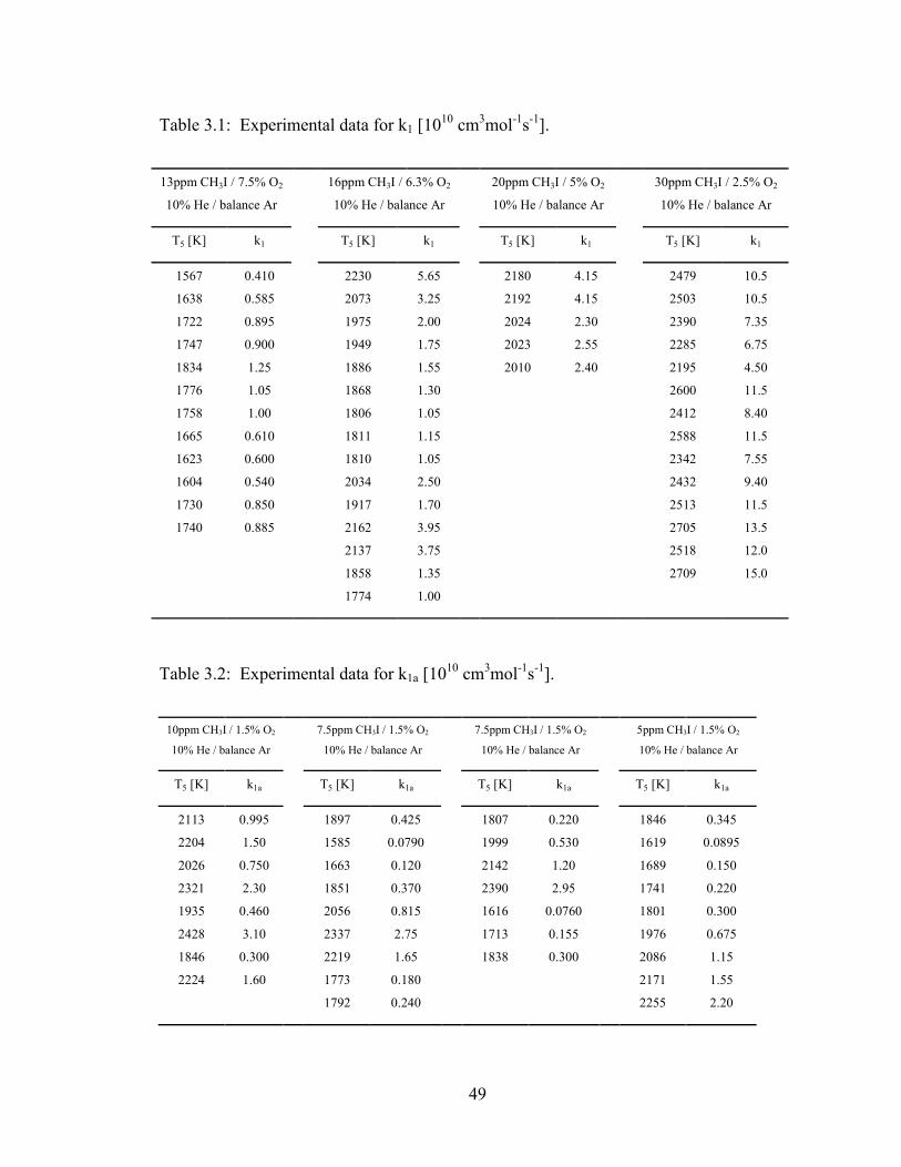
49

Table 3.1: Experimental data for k1 [1010 cm3mol-1s-1].

13ppm CH3I / 7.5% O2 16ppm CH3I / 6.3% O2 20ppm CH3I / 5% O2 30ppm CH3I / 2.5% O2

10% He / balance Ar 10% He / balance Ar 10% He / balance Ar 10% He / balance Ar

T5 [K] k1 T5 [K] k1 T5 [K] k1 T5 [K] k1

1567 0.410 2230 5.65 2180 4.15 2479 10.5

1638 0.585 2073 3.25 2192 4.15 2503 10.5

1722 0.895 1975 2.00 2024 2.30 2390 7.35

1747 0.900 1949 1.75 2023 2.55 2285 6.75

1834 1.25 1886 1.55 2010 2.40 2195 4.50

1776 1.05 1868 1.30 2600 11.5

1758 1.00 1806 1.05 2412 8.40

1665 0.610 1811 1.15 2588 11.5

1623 0.600 1810 1.05 2342 7.55

1604 0.540 2034 2.50 2432 9.40

1730 0.850 1917 1.70 2513 11.5

1740 0.885 2162 3.95 2705 13.5

2137 3.75 2518 12.0

1858 1.35 2709 15.0

1774 1.00

Table 3.2: Experimental data for k1a [1010 cm3mol-1s-1].

10ppm CH3I / 1.5% O2 7.5ppm CH3I / 1.5% O2 7.5ppm CH3I / 1.5% O2 5ppm CH3I / 1.5% O2

10% He / balance Ar 10% He / balance Ar 10% He / balance Ar 10% He / balance Ar

T5 [K] k1a T5 [K] k1a T5 [K] k1a T5 [K] k1a

2113 0.995 1897 0.425 1807 0.220 1846 0.345

2204 1.50 1585 0.0790 1999 0.530 1619 0.0895

2026 0.750 1663 0.120 2142 1.20 1689 0.150

2321 2.30 1851 0.370 2390 2.95 1741 0.220

1935 0.460 2056 0.815 1616 0.0760 1801 0.300

2428 3.10 2337 2.75 1713 0.155 1976 0.675

1846 0.300 2219 1.65 1838 0.300 2086 1.15

2224 1.60 1773 0.180 2171 1.55

1792 0.240 2255 2.20

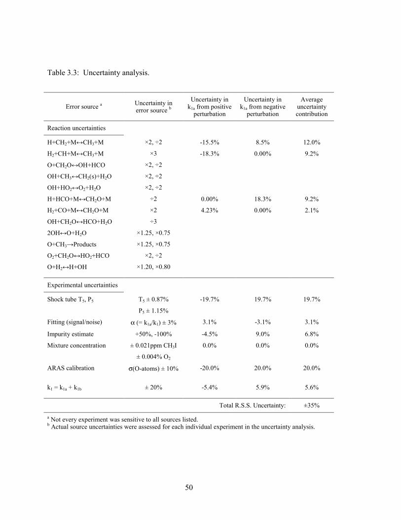
50

Table 3.3: Uncertainty analysis.

Error source a Uncertainty in error source b

Uncertainty in k1a from positive

perturbation

Uncertainty in k1a from negative

perturbation

Average uncertainty contribution

Reaction uncertainties H+CH2+M↔CH3+M ×2, ÷2 -15.5% 8.5% 12.0%

H2+CH+M↔CH3+M ×3 -18.3% 0.00% 9.2%

O+CH2O↔OH+HCO ×2, ÷2

OH+CH3↔CH2(s)+H2O ×2, ÷2

OH+HO2↔O2+H2O ×2, ÷2

H+HCO+M↔CH2O+M ÷2 0.00% 18.3% 9.2%

H2+CO+M↔CH2O+M ×2 4.23% 0.00% 2.1%

OH+CH2O↔HCO+H2O ÷3

2OH↔O+H2O ×1.25, ×0.75

O+CH3→Products ×1.25, ×0.75

O2+CH2O↔HO2+HCO ×2, ÷2

O+H2↔H+OH ×1.20, ×0.80 Experimental uncertainties Shock tube T5, P5 T5 ± 0.87%

P5 ± 1.15%

-19.7% 19.7% 19.7%

Fitting (signal/noise) α (= k1a/k1) ± 3%

3.1% -3.1% 3.1%

Impurity estimate +50%, -100% -4.5% 9.0% 6.8%

Mixture concentration ± 0.021ppm CH3I

± 0.004% O2

0.0% 0.0% 0.0%

ARAS calibration σ(O-atoms) ± 10% -20.0% 20.0% 20.0%

k1 = k1a + k1b ± 20% -5.4% 5.9% 5.6% Total R.S.S. Uncertainty: ±35% a Not every experiment was sensitive to all sources listed. b Actual source uncertainties were assessed for each individual experiment in the uncertainty analysis.

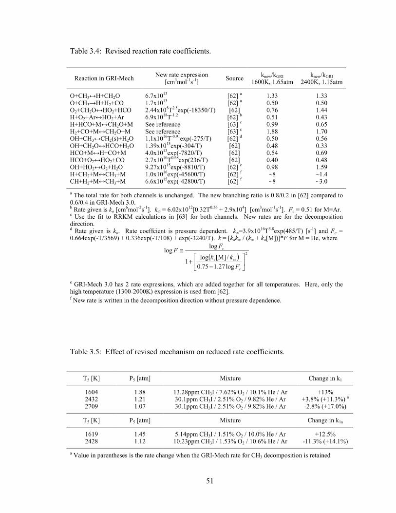
51

Table 3.4: Revised reaction rate coefficients.

knew/kGRI knew/kGRI Reaction in GRI-Mech New rate expression

[cm3mol-1s-1] Source 1600K, 1.65atm 2400K, 1.15atm O+CH3↔H+CH2O 6.7x1013 [62] a 1.33 1.33 O+CH3→H+H2+CO 1.7x1013 [62] a 0.50 0.50 O2+CH2O↔HO2+HCO 2.44x105T2.5exp(-18350/T) [62] 0.76 1.44 H+O2+Ar↔HO2+Ar 6.9x1018T-1.2 [62] b 0.51 0.43 H+HCO+M↔CH2O+M See reference [63] c 0.99 0.65 H2+CO+M↔CH2O+M See reference [63] c 1.88 1.70 OH+CH3↔CH2(s)+H2O 1.1x1016T-0.91exp(-275/T) [62] d 0.50 0.56 OH+CH2O↔HCO+H2O 1.39x1013exp(-304/T) [62] 0.48 0.33 HCO+M↔H+CO+M 4.0x1013exp(-7820/T) [62] 0.54 0.69 HCO+O2↔HO2+CO 2.7x1010T0.68exp(236/T) [62] 0.40 0.48 OH+HO2↔O2+H2O 9.27x1015exp(-8810/T) [62] e 0.98 1.59 H+CH2+M↔CH3+M 1.0x1016exp(-45600/T) [62] f ~8 ~1.4 CH+H2+M↔CH3+M 6.6x1015exp(-42800/T) [62] f ~8 ~3.0 a The total rate for both channels is unchanged. The new branching ratio is 0.8/0.2 in [62] compared to 0.6/0.4 in GRI-Mech 3.0. b Rate given is ko [cm6mol-2s-1]. k∞ = 6.02x1012[0.32T0.56 + 2.9x104] [cm3mol-1s-1]. Fc = 0.51 for M=Ar. c Use the fit to RRKM calculations in [63] for both channels. New rates are for the decomposition direction. d Rate given is ko. Rate coeffcient is pressure dependent. k∞=3.9x1016T5.8exp(485/T) [s-1] and Fc = 0.664exp(-T/3569) + 0.336exp(-T/108) + exp(-3240/T). k = [kok∞ / (k∞ + ko[M])]*F for M = He, where

( ) 2

log27.175.0/]M[log

1

loglog

−+

≅∞

c

c

Fkk

FF�

e GRI-Mech 3.0 has 2 rate expressions, which are added together for all temperatures. Here, only the high temperature (1300-2000K) expression is used from [62]. f New rate is written in the decomposition direction without pressure dependence.

Table 3.5: Effect of revised mechanism on reduced rate coefficients.

T5 [K] P5 [atm] Mixture Change in k1 1604 1.88 13.28ppm CH3I / 7.62% O2 / 10.1% He / Ar +13% 2432 1.21 30.1ppm CH3I / 2.51% O2 / 9.82% He / Ar +3.8% (+11.3%) a

2709 1.07 30.1ppm CH3I / 2.51% O2 / 9.82% He / Ar -2.8% (+17.0%) T5 [K] P5 [atm] Mixture Change in k1a 1619 1.45 5.14ppm CH3I / 1.51% O2 / 10.0% He / Ar +12.5% 2428 1.12 10.23ppm CH3I / 1.53% O2 / 10.6% He / Ar -11.3% (+14.1%)

a Value in parentheses is the rate change when the GRI-Mech rate for CH3 decomposition is retained

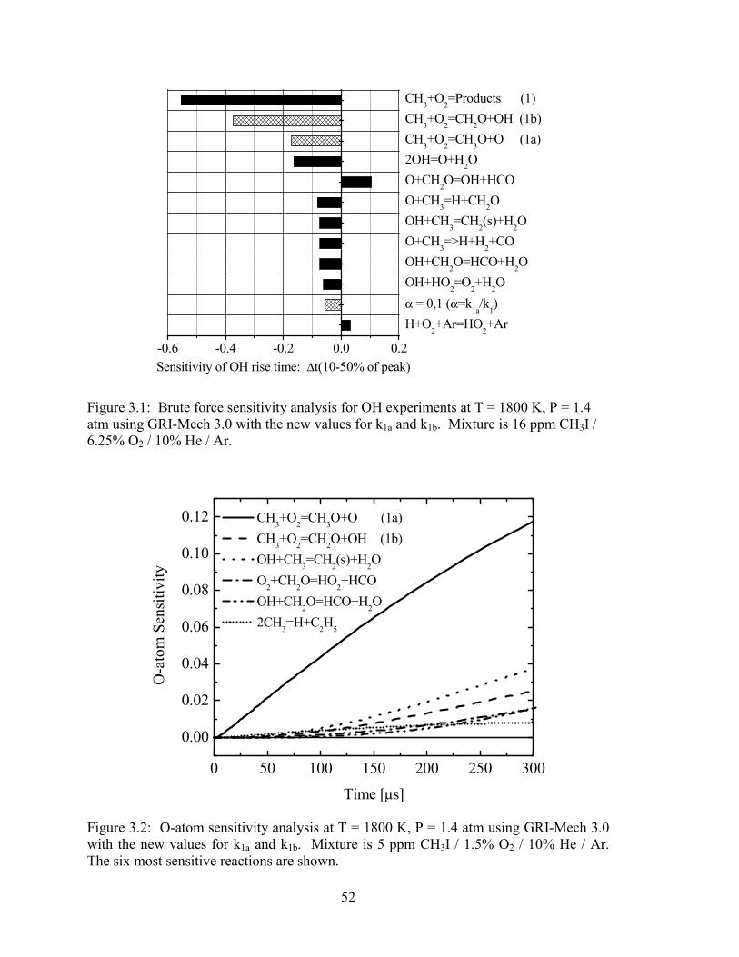
52

-0.6 -0.4 -0.2 0.0 0.2

Sensitivity of OH rise time: ∆t(10-50% of peak)

CH3+O2=Products (1)CH3+O2=CH2O+OH (1b) CH3+O2=CH3O+O (1a) 2OH=O+H2O O+CH2O=OH+HCO O+CH3=H+CH2O OH+CH3=CH2(s)+H2O O+CH3=>H+H2+CO OH+CH2O=HCO+H2O OH+HO2=O2+H2O α = 0,1 (α=k1a/k1)H+O2+Ar=HO2+Ar

Figure 3.1: Brute force sensitivity analysis for OH experiments at T = 1800 K, P = 1.4 atm using GRI-Mech 3.0 with the new values for k1a and k1b. Mixture is 16 ppm CH3I / 6.25% O2 / 10% He / Ar.

0 50 100 150 200 250 300

0.00

0.02

0.04

0.06

0.08

0.10

0.12 CH3+O2=CH3O+O (1a) CH3+O2=CH2O+OH (1b) OH+CH3=CH2(s)+H2O O2+CH2O=HO2+HCO OH+CH2O=HCO+H2O 2CH3=H+C2H5

O-a

tom

Sen

sitiv

ity

Time [µs]

Figure 3.2: O-atom sensitivity analysis at T = 1800 K, P = 1.4 atm using GRI-Mech 3.0 with the new values for k1a and k1b. Mixture is 5 ppm CH3I / 1.5% O2 / 10% He / Ar. The six most sensitive reactions are shown.

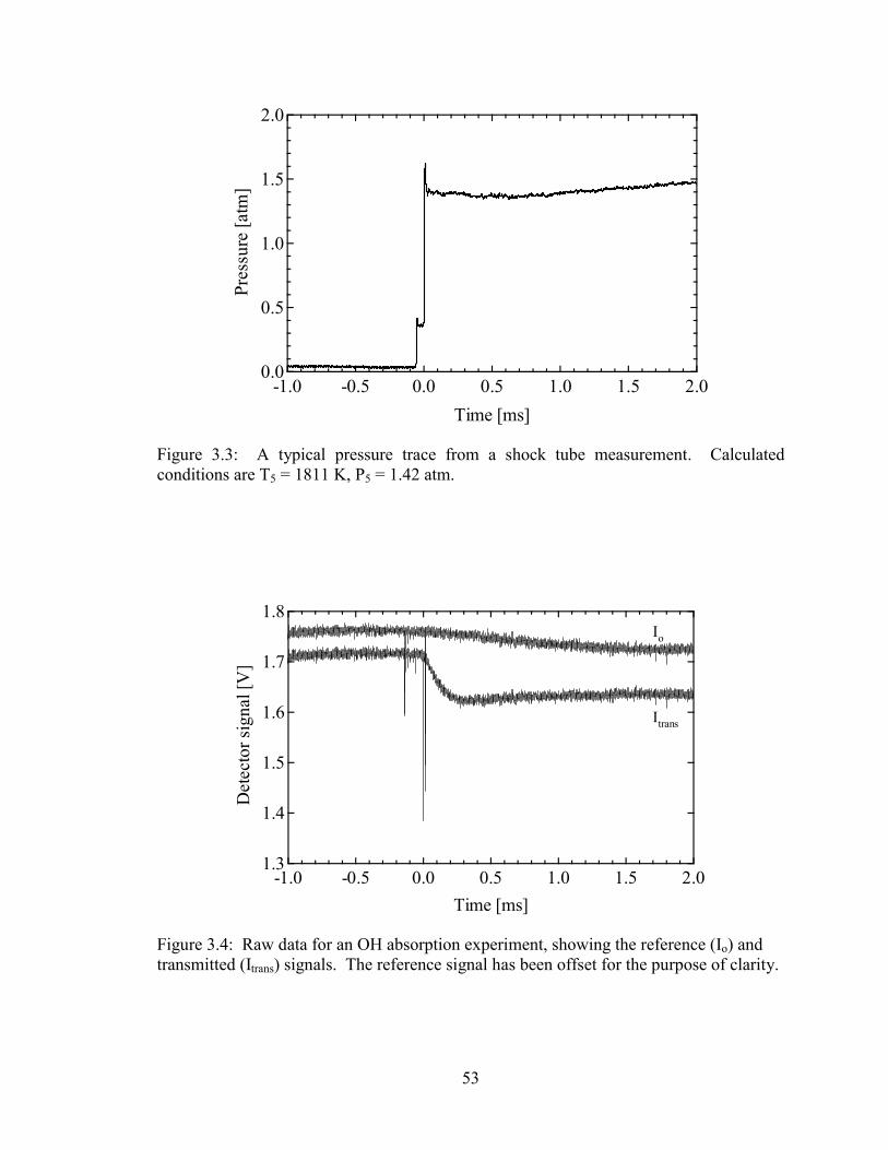
53

2.0

1.5

1.0

0.5

0.0

Pres

sure

[atm

]

2.01.51.00.50.0-0.5-1.0Time [ms]

Figure 3.3: A typical pressure trace from a shock tube measurement. Calculated conditions are T5 = 1811 K, P5 = 1.42 atm.

1.8

1.7

1.6

1.5

1.4

1.3

Det

ecto

r sig

nal [

V]

2.01.51.00.50.0-0.5-1.0Time [ms]

Io

Itrans

Figure 3.4: Raw data for an OH absorption experiment, showing the reference (Io) and transmitted (Itrans) signals. The reference signal has been offset for the purpose of clarity.

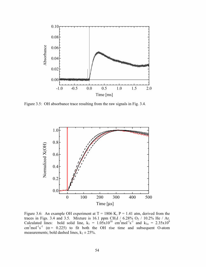
54

0.10

0.08

0.06

0.04

0.02

0.00

Abs

orba

nce

2.01.51.00.50.0-0.5-1.0Time [ms]

Figure 3.5: OH absorbance trace resulting from the raw signals in Fig. 3.4.

1.0

0.8

0.6

0.4

0.2

0.0

Nor

mal

ized

Χ(O

H)

5004003002001000Time [µs]

Figure 3.6: An example OH experiment at T = 1806 K, P = 1.41 atm, derived from the traces in Figs. 3.4 and 3.5. Mixture is 16.1 ppm CH3I / 6.28% O2 / 10.2% He / Ar. Calculated lines: bold solid line, k1 = 1.05x1010 cm3mol-1s-1 and k1a = 2.35x109 cm3mol-1s-1 (α = 0.225) to fit both the OH rise time and subsequent O-atom measurements; bold dashed lines, k1 ± 25%.

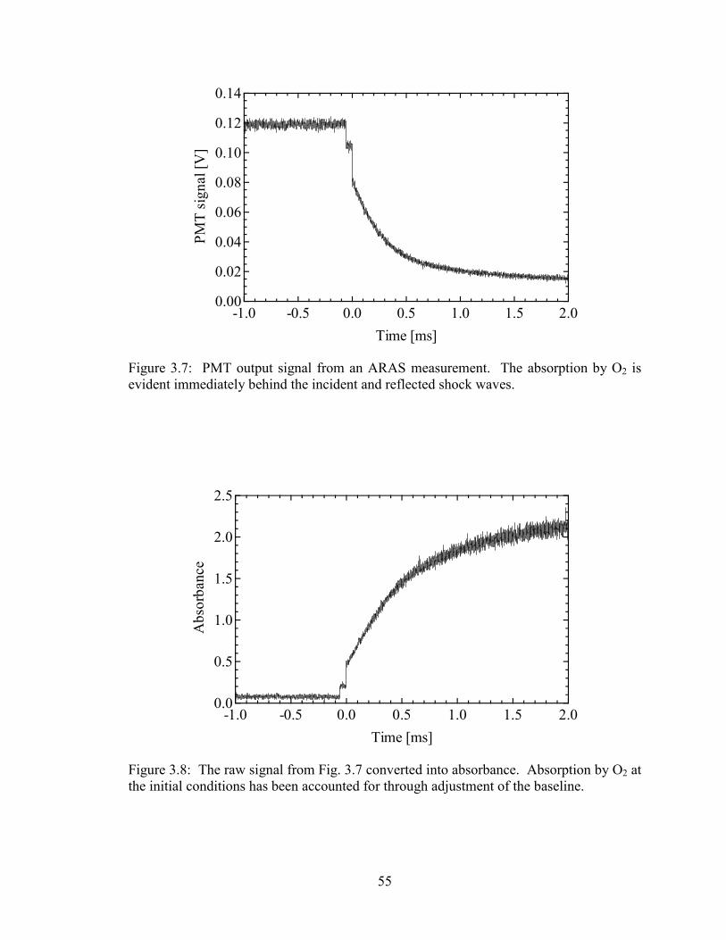
55

0.14

0.12

0.10

0.08

0.06

0.04

0.02

0.00

PMT

sign

al [V

]

2.01.51.00.50.0-0.5-1.0Time [ms]

Figure 3.7: PMT output signal from an ARAS measurement. The absorption by O2 is evident immediately behind the incident and reflected shock waves.

2.5

2.0

1.5

1.0

0.5

0.0

Abs

orba

nce

2.01.51.00.50.0-0.5-1.0Time [ms]

Figure 3.8: The raw signal from Fig. 3.7 converted into absorbance. Absorption by O2 at the initial conditions has been accounted for through adjustment of the baseline.

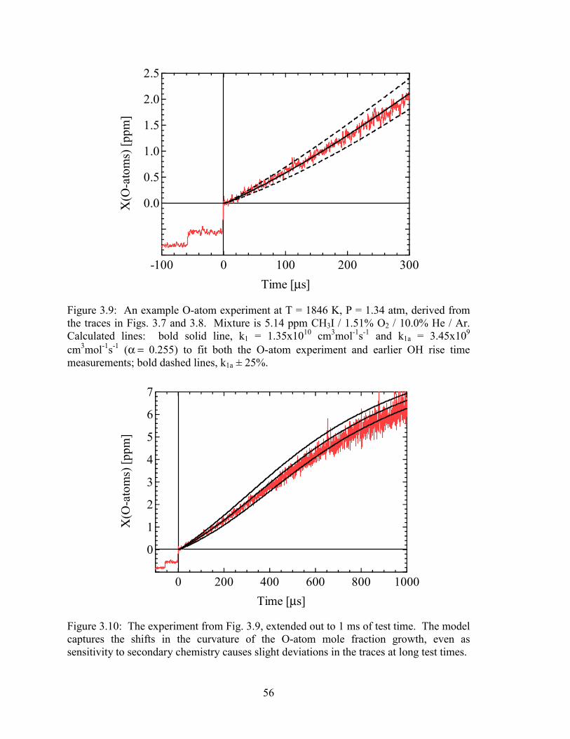
56

2.5

2.0

1.5

1.0

0.5

0.0

-0.5

-1.0

Χ(O

-ato

ms)

[ppm

]

3002001000-100Time [µs]

Figure 3.9: An example O-atom experiment at T = 1846 K, P = 1.34 atm, derived from the traces in Figs. 3.7 and 3.8. Mixture is 5.14 ppm CH3I / 1.51% O2 / 10.0% He / Ar. Calculated lines: bold solid line, k1 = 1.35x1010 cm3mol-1s-1 and k1a = 3.45x109 cm3mol-1s-1 (α = 0.255) to fit both the O-atom experiment and earlier OH rise time measurements; bold dashed lines, k1a ± 25%.

7

6

5

4

3

2

1

0

-1

Χ(O

-ato

ms)

[ppm

]

10008006004002000Time [µs]

Figure 3.10: The experiment from Fig. 3.9, extended out to 1 ms of test time. The model captures the shifts in the curvature of the O-atom mole fraction growth, even as sensitivity to secondary chemistry causes slight deviations in the traces at long test times.

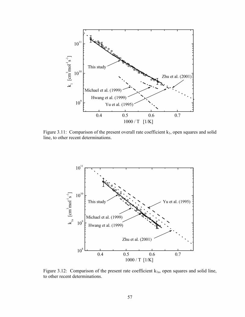
57

0.4 0.5 0.6 0.7

109

1010

1011

This study

Yu et al. (1995) Hwang et al. (1999)

Zhu et al. (2001)

k 1 [cm

3 mol

-1s-1

]

1000 / T [1/K]

Michael et al. (1999)

Figure 3.11: Comparison of the present overall rate coefficient k1, open squares and solid line, to other recent determinations.

0.4 0.5 0.6 0.7108

109

1010

1011

Zhu et al. (2001)

Yu et al. (1995)

Hwang et al. (1999)

Michael et al. (1999)

This study

k 1a [

cm3 m

ol-1

s-1]

1000 / T [1/K]

Figure 3.12: Comparison of the present rate coefficient k1a, open squares and solid line, to other recent determinations.

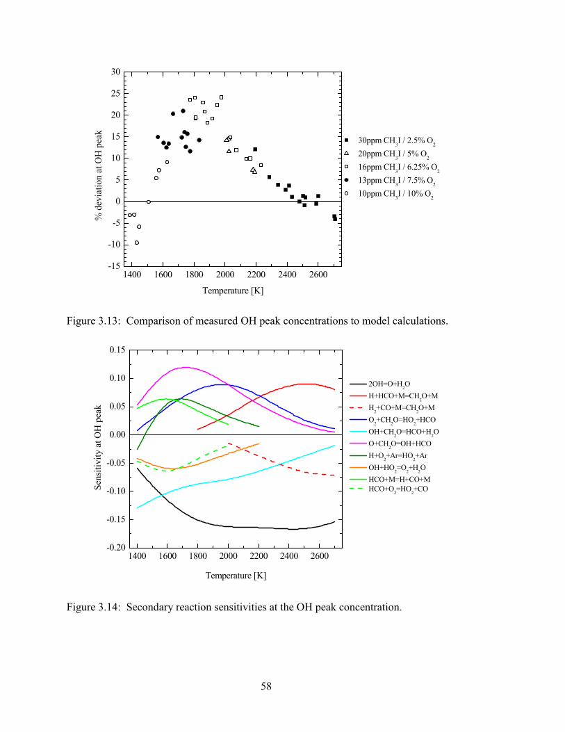
58

1400 1600 1800 2000 2200 2400 2600-15

-10

-5

0

5

10

15

20

25

30

% d

evia

tion

at O

H p

eak

Temperature [K]

30ppm CH3I / 2.5% O2

20ppm CH3I / 5% O2

16ppm CH3I / 6.25% O2

13ppm CH3I / 7.5% O2

10ppm CH3I / 10% O2

Figure 3.13: Comparison of measured OH peak concentrations to model calculations.

1400 1600 1800 2000 2200 2400 2600-0.20

-0.15

-0.10

-0.05

0.00

0.05

0.10

0.15

Sens

itivi

ty a

t OH

pea

k

Temperature [K]

2OH=O+H2O H+HCO+M=CH2O+M H2+CO+M=CH2O+M O2+CH2O=HO2+HCO OH+CH2O=HCO+H2O O+CH2O=OH+HCO H+O2+Ar=HO2+Ar OH+HO2=O2+H2O HCO+M=H+CO+M HCO+O2=HO2+CO

Figure 3.14: Secondary reaction sensitivities at the OH peak concentration.

59

Chapter 4: The heat of formation of OH

This chapter details a high-temperature measurement of the standard heat of

formation of OH, ∆fH°298(OH), using a shock tube. The unique experimental approach is

presented, and the results are discussed and compared to previous values of the heat of

formation.

4.1 Introduction Various methods have been utilized to determine the heat of formation of OH and

are briefly discussed in Chapter 1. In contrast to experimental studies at room

temperature, the present work makes use of the partial equilibrium of reactions involving

the OH radical behind reflected shock waves in H2/O2/Ar mixtures. In the partial

equilibrium state, calculated OH concentrations are sensitive primarily to thermodynamic

parameters and not reaction rates. Details on the partial equilibrium model can be found

in Appendix E.

Six major species participate in the partial equilibrium state in H2 / O2 mixtures.

Table 4.1 shows the heats of formation for these six species and an evaluation of their

uncertainties [28]. Of the thermochemical parameters for these six species, ∆fH°298(OH)

has by far the largest uncertainty. The heat of formation of OH may therefore serve as a

fitting parameter in comparisons of measured OH profiles to those calculated with either

a kinetic mechanism or using the partial equilibrium model, with very little error due to

uncertainties in other thermochemical parameters.

4.2 Experimental apparatus All experiments in this thesis were carried out in the shock tube facility described

in Chapter 2. Concentration time-histories of OH were measured using cw laser

60

absorption of the R1(5) transition in the A-X(0,0) system near 306.7 nm as described in

Section 2.2.

4.3 Review of OH spectral absorption coefficients In the initial phase of the current work, a review of recent OH spectroscopic and

molecular data was undertaken, and the method for calculating absolute absorption

coefficients was carefully scrutinized. The absorption of spectrally narrow laser radiation

as it passes through a uniform volume containing an absorbing species is related to the

concentration of the species through the Beer-Lambert relation:

( )LΧPkIIT OHtotνo

ν −== exp (4.1)

Here Tν is the fractional transmission at frequency ν, Io is the incident power, I is the

transmitted power, kν is the spectral absorption coefficient, Ptot the total pressure, L the

path length, and ΧOH the mole fraction of OH. The absorption coefficient is the product

of the integrated line strength, Slu, and the line shape function φ(ν): kν = Slu*φ(ν). The

line strength of a given transition is dependent on temperature and molecular properties

alone, whereas the line shape function is dependent on temperature, pressure, and

collision partner species, with the functional dependencies changing for different

transitions [71]. The integrated line strength can be most easily calculated in the form

given by Goldman and Gillis [72]:

( ) ( ) ( ) ( )[ ]/T .--J'AQ

/TE .-PN

πcνTS ul

totOHlu ν43881exp11243881exp

81

2 +′′

= (4.2)

Here J’ is the upper-state rotational quantum number. In this equation, parameters that

must come from measured or calculated values found in the literature are the transition

frequency, ν, the lower-state rotational energy term value, E”, the Einstein A-coefficient,

Aul, and the total internal partition function, Qtot. The most precise measurements of

transition frequencies in the (0,0) band of the A-X system of OH have been performed by

Stark et al. [73], which, at least for the R1(5) transition, have not changed significantly

from the earlier values given in Goldman and Gillis [72]. The values for E” and Aul (up

to v” = 2) have been recently tabulated [74], the values for Aul coming from calculations

61

of relative transition probabilities [75] which are set on an absolute scale through an

earlier radiative lifetime measurement [76] and tabulated in a software program [77].

The values for E” are for the present purposes indistinguishable from those calculated

and tabulated earlier in [72] and [73].

The total internal partition function, Qtot, requires careful attention. Various

levels of approximation are often invoked when calculating the partition function or its

components, particularly if the different components are calculated separately

(Qtot=QelecQrotQvib) without proper regard for anharmonicity, vibration-rotation

interaction, spin-splitting, and lambda-doubling. In the current work, only full

summations over all relevant energy states or accurate polynomial representations of such

summations were used in the calculation of the total internal partition function. The

vibrational and electronic/rotational energies are calculated separately and added together

for the final partition function summation. For the vibrational term values, fitted and

tabulated Dunham coefficients [75] are used to calculate the vibrational term values up to

v” = 13. For the electronic/rotational component, the energy term values are calculated

up to J” = 40.5, using the appropriate formulas for the inverted, spin-split, lambda-

doubled X2Π ground state [78] and molecular constants [75,79], including vibration-

rotation interaction. The vibrational and electronic/rotational energy term values are

added together, and a partition function summation is performed over all energy levels,

up to J” = 40.5 and v” = 8, or enough to converge for the given experimental conditions.

A Voigt line shape profile is used for calculating the absorption coefficient at a

given wavelength, utilizing the measured collision broadening [39] and collision shift

coefficients (see Appendix B) for Ar. The collision width was verified in new

experiments using Rea’s rapid-tuning technique [40] and found to lie within the

combined error limits (see Appendix B). Uncertainty in the collision width is taken as

the limits of the uncertainty bars in [39], ~ ± 12%. Uncertainty in the collision shift has a

negligible effect on the measured OH mole fraction at the conditions of this study.

4.4 Experimental conditions The experiments were designed to be sensitive primarily to thermochemical

parameters, rather than reaction rate coefficients, by taking advantage of the partial

62

equilibrium state occurring at the end of the ignition process. Gas mixtures were

prepared manometrically in a stainless steel mixing cylinder and mechanically mixed

with a magnetically driven stirrer. Component gases were high-purity H2 (99.999%), O2

(99.993%), and Ar (99.998%). Reactant mixture composition was chosen on the basis of

several factors. For good signal-to-noise and resolution, experiments ideally involved

40-80% peak absorption. To maintain confidence in the post-shock conditions, OH

induction times were kept below 200 µs, and typically were much shorter. Mixtures were

restricted to low concentrations to reduce effects of energy release. Finally,

stoichiometries of Φ=0.5 (4000 ppm H2 / 4000 ppm O2 / balance Ar) and Φ=1.0 (8000

ppm H2 / 4000 ppm O2 / balance Ar) were used for the above reasons as well as their low

sensitivities to reaction rate coefficients. Very rich or very lean mixtures display

significantly increased sensitivity of the plateau ΧOH to various rate coefficients, even at

conditions producing a fairly flat “plateau”. The chosen stoichiometries provided a

reasonably flat or slowly decaying OH profile over a somewhat broad range of

temperatures.

4.5 Data and results

4.5.1 Experiments

In the present work, reflected-shock temperatures ranged from 1964 to 2718 K.

Pressures typically ranged from 1 to 1.4 atm; however, one set of experiments was

performed at higher pressures up to 2.4 atm to ensure insensitivity of the evaluated

∆fH°298(OH) to pressure. One additional experiment was also conducted using the R1(6)

absorption transition to check consistency of the spectroscopic database. Finally, a series

of experiments was performed in which the laser frequency was rapidly tuned over the

full lineshape. These data allowed us to verify the broadening coefficients, and the peak

absorption of the lineshape provided an additional measurement of the OH plateau for

comparison to fixed-frequency experiments.

Results of a typical fixed-frequency shock tube experiment are shown in Fig. 4.1.

After a brief induction period the OH concentration rapidly increases and achieves a

plateau value. At the conditions of Fig. 4.1, only a very slight decay of the OH is visible

63

during the test time. The measured OH mole fraction, ΧOH, is compared to a model

calculation at constant T, P conditions. For the purposes of modeling the OH traces, the

mechanism used was the H2-O2 subset of GRI-Mech 3.0 [2], along with its

thermodynamic database. Other thermodynamics databases also were used in data

reduction for comparison purposes. Calculations were performed using the Chemkin-II

chemical kinetics simulation package [53].

4.5.2 Fitting the data

Each experiment was individually fit by adjusting the heat of formation of OH in

the model thermodynamics until the calculated OH plateau matched the measured OH

peak/plateau. In the NASA polynomial representation of Cp(T) [80], a sixth term (a6) is

introduced as the integration constant for the calculation of H(T):

TaTaTaTaTaa

RTH o

64

5

3

4

2

321 5432+++++= (4.3)

This term is independent of temperature and therefore represents a constant offset in the

enthalpy H(T) for all temperatures. Fitting the model to the data involved adjustment of

a6 in the high temperature polynomial. The overall goodness of the fit is evident in Fig.

4.1. The effective change in a6 (from its original value) was applied to the a6 term in the

low temperature polynomial. This adjusted low temperature polynomial was then used to

calculate H(298) = ∆fH°298(OH). For the experiment of Fig. 4.1, ∆fH°298(OH) changed

from the GRI-Mech 3.0 value of 9.403 kcal/mol to 8.887 kcal/mol.

4.5.3 Uncertainty analysis

A thorough uncertainty analysis was carried out for each of four experiments

representing the full range of experimental conditions: high temperature, lower

temperature, and higher pressure (all at Φ = 0.5), and one experiment for Φ = 1. For a

given source of error, the uncertainty is applied to the data reduction and carried through

to a change in the ΧOH(measured) vs. ΧOH(model). The various sources of error affected

either the reduction of the raw absorption data to ΧOH, the calculation of ΧOH, or both.

The difference in the offset of each of the measured and calculated peak OH mole

fractions then represents the uncertainty in fitting the measured OH mole fraction due to

64

this source of error. The uncertainty in mole fraction from each source was combined

with the uncertainty from all other sources of error in the peak mole fraction, assuming

uncorrelated uncertainties. Finally, the combined total uncertainty in ΧOH is used to

define an uncertainty in ∆fH°298(OH) for the given experiment.

The major sources of uncertainty and their effect on ∆fH°298(OH) are displayed in

Figs. 4.2 and 4.3 for conditions near the experimental high- and low-temperature limits.

For the nominal conditions (the conditions of Figs. 4.1 and 4.2) the dominant source of

uncertainty is the absolute absorption linestrength (± 2σ error = ± 2%). However, at

lower temperatures and higher pressures, uncertainty in the collision-broadened linewidth

becomes more important and contributes almost half of the total uncertainty. For

linestrength, collision broadening, and collision shift, the uncertainty is taken directly

from that reported in the literature and Appendix B. Uncertainty in the measured shock

velocity was based on the measured variations in pressure transducer response and the

quality of the shock trajectory fit, and was propagated through to uncertainties in T5 and

P5 and on to an uncertainty in ∆fH°298(OH) (see Appendix C).

Uncertainty due to (or rather sensitivity to) reaction rate coefficients was

determined by adjusting each individual rate coefficient in turn and determining its effect

on the OH peak, with error limits taken from Baulch et al. [81] or more recent

measurements/literature reviews. These calculations are plotted as a function of

temperature in Fig. 4.4. It is clear from Figs. 4.2 and 4.3 that kinetics play no significant

role in the determination of the peak mole fraction at these conditions. At the lower-

temperature conditions of Fig. 4.3, the OH decays slightly faster and therefore the peak

OH shows some increased sensitivity to the kinetics; however, the kinetic sensitivity is

still negligible compared to the absorption linestrength and collision-broadening

uncertainties. Below 1950K, sensitivity to kinetic rate coefficients rises significantly,

thus setting the low-temperature limit for this experimental measurement strategy.

4.5.4 Results

Values of the heat of formation derived using the above methods are shown for all

experiments in Fig. 4.5. Representative error bars are given for the two experiments of

Figs. 4.2 and 4.3. Also displayed are lines representing the older and most recently used

65

values for ∆fH°298(OH) found in several databases. The Sandia database [82]

incorporates ∆fH°298(OH) = 9.32 kcal/mol taken directly from the NIST-JANAF tables

[32]. GRI-Mech 3.0 [37] uses ∆fH°298(OH) = 9.40 kcal/mol, which is the same as in the

tables of Gurvich et al. [31]. The database by Burcat [83] uses ∆fH°298(OH) = 8.97

kcal/mol, which is calculated based on ∆fH°0(OH) = 8.83 kcal/mol [29] but uses a NASA

polynomials and coefficients code (PAC) for the enthalpy increments [83,84]. The mean

value over all our experiments is ∆fH°298(OH) = 8.92 kcal/mol (37.3 kJ/mol). This

number is in close agreement with the value of Ruscic et al. [30], ∆fH°298(OH) = 8.91 ±

0.07 kcal/mol (37.3 ± 0.29 kJ/mol). Over the four experiments where detailed

uncertainty analysis has been performed, the uncertainty assigned to our value is, on

average, ± 0.16 kcal/mol (± 0.67 kJ/mol). Standard deviation from the mean (taken over

all experiments) is 0.04 kcal/mol (0.17 kJ/mol).

To check for sensitivity to thermodynamic parameters other than ∆fH°298(OH),

two other chemical kinetics thermodynamics databases were used to reduce all

experiments. The change in the reduced ∆fH°298(OH) using these different databases is

shown in Fig. 4.6. The average value of ∆fH°298(OH) obtained using the Sandia database

[82] was 0.01 kcal/mol higher, where the value inferred using the Burcat database [83]

was 0.003 kcal/mol lower. Over the temperature range of the present measurements, the

difference among these three databases increases monotonically with temperature so that

the difference in the value of ∆fH°298(OH) derived using Sandia vs GRI-Mech 3.0

thermodynamics actually ranges from 0.003 to 0.018 kcal/mol over 1964-2718K. The

difference using the Burcat vs. GRI-Mech 3.0 database ranges from -0.002 to -0.007

kcal/mol. This systematic variation in the reduced ∆fH°298(OH) with temperature is

suggestive of differences in thermodynamic parameters due to varying levels of

approximations used in their calculation. The similarities between the reduced values

using the three databases indicate relatively good agreement for the thermodynamics and

thermochemistry of the other species involved (H2, O2, H, O, and H2O) as well as the

sensible enthalpy and entropy calculations for OH.

66

4.6 Discussion

4.6.1 Verification of the sensible enthalpy

Because the experiments are fit at high temperatures, care must be taken to ensure

the accuracy of the integration of the specific heat, Cp, from 298 K to the experimental

temperature. An error in the sensible enthalpy, H(T)-H(298), would lead directly to an

error in the reduced ∆fH°298(OH). To examine the magnitude of this error, the total

internal partition function, calculated previously, was used in the following formula to

calculate H(T):

( )RT

dTQdRTTH

25ln

)( int2 +

= (4.4)

This calculation provided two interesting results. First, as asserted by Ruscic et al.

[29,30] and given in tables by Gurvich et al. [31], the present calculation confirmed that

the difference between ∆fH°0 and ∆fH°298 should be 0.06 kcal/mol, rather than the 0.14

kcal/mol in the NIST-JANAF table [32]. The NIST-JANAF table points out this

discrepancy in the discussion, indicating that H(0 K) – H(298 K) should be –2.107

kcal/mol (- 8.816 kJ/mol), not -2.192 kcal/mol (-9.172 kJ/mol) as given in the actual

tables. Second, the current calculation of H(T)-H(298) up to high temperatures (at least

3000K) yields excellent agreement with the careful calculations and tabulations of

Gurvich et al. [31] and the polynomial fit expressions in the GRI-Mech 3.0

thermodynamics. At the highest temperature of the present study (2700K), the other

three databases [32,82,83], agree with each other but are 0.03 kcal/mol lower than the

present calculation. One might expect, therefore, that fitting the experimental OH data

using these other databases may result in a maximum deviation of ∆fH°298(OH) on the

order of 0.03 kcal/mol.

4.6.2 The OH absorption oscillator strength

The dominant uncertainty at the nominal conditions (see Fig. 4.2) is the

absorption oscillator strength. While relative transition probabilities can now be

calculated with high accuracy [75], the limitation on the oscillator strength is the

measurement of the radiative lifetime of OH. Many measurements of this parameter have

67

been made; however, the value most often quoted is that by German [76], τrad = 688 ± 14

ns, where the uncertainty limits are ± 2σ = ± 2%. This uncertainty transfers directly to a

± 2% uncertainty in the absolute oscillator strength. An independent study by Dimpfl

and Kinsey [85] has confirmed this lifetime measurement, yielding a published value of

686 ± 14 ns. The present work has retained the ± 2% error bounds of German [76] in

our own uncertainty analysis for ∆fH°298(OH).

It can be shown that any source of error which has a constant temperature-

independent fractional effect on the measured OH concentration, such as an error in Slu or

the absorption pathlength, when applied across the whole temperature range of

experiments would impact the data reduction of ∆fH°298(OH) in such a way as to create a

temperature-varying value for ∆fH°298(OH). This is unphysical, and is a primary reason

why data were taken over a range of temperatures. As no temperature dependence is

evident in Fig. 4.5, the data provide relative assurance that any error in the integrated line

strength is small enough to be hidden within the data scatter and other uncertainty

sources.

4.6.3 Comparison to previous work

From Fig. 4.5, it is clear that the current work agrees with the most recent value of

∆fH°(OH) from Ruscic et al. [30]. Their recommendation is ∆fH°0(OH) = 8.85 ± 0.07

kcal/mol (37.0 ± 0.29 kJ/mol), yielding a value at 298K of ∆fH°298(OH) = 8.91 ± 0.07

kcal/mol (37.3 ± 0.29 kJ/mol). Another recent study utilizes thermochemical cycle

analysis alone to arrive at a similar value of ∆fH°0(OH) = 8.88 ± 0.03 kcal/mol (37.14 ±

0.12 kJ/mol), yielding a value at 298K of ∆fH°298(OH) = 8.94 ± 0.03 kcal/mol (37.4 ±

0.12 kJ/mol) [35]. The present study, using a method quite different from that of either

[30] or [35], has found agreement with the new lower value for ∆fH°298(OH) given by

both [30] and [35]. As in both other studies, the uncertainty in the present study is less

than half of the difference between the old and new values, clearly differentiating it from

the previous high values. Taking the average of all three studies, weighted by their

uncertainties, yields a recommended value of ∆fH°298(OH) = 8.93 kcal/mol, with an

uncertainty of ~±0.07 kcal/mol.

68

4.6.4 Implications

The reported change in ∆fH°(OH) translates to a factor of exp[-δ(∆Hof)/RT]

change in rate parameters deduced from equilibrium constants and, of course, to

equilibrium constants themselves. In addition, if the value for OH is used to deduce

thermochemical parameters of other species, those parameters will also be affected.

Some of these effects have been discussed by others [30,35].

4.7 Conclusions The standard heat of formation of OH, ∆fH°298(OH), has been determined from

high temperature shock tube experiments. Measurements over the temperature range

1964 to 2718 K yielded an average determination of ∆fH°298(OH) = 8.92 ± 0.16 kcal/mol

(37.3 ± 0.67 kJ/mol), with a standard deviation in the measurement of σ = 0.04 kcal/mol

(0.17 kJ/mol). The current study agrees very well with two other recent determinations

of ∆fH°0(OH) and corroborates the suggestion that the previously accepted values,

∆fH°298(OH) = 9.32-9.4 kcal/mol, are in error.

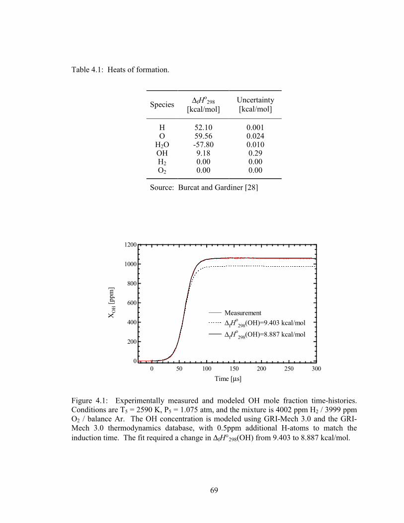
69

Table 4.1: Heats of formation.

Species ∆fHo298

[kcal/mol] Uncertainty [kcal/mol]

H 52.10 0.001O 59.56 0.024

H2O -57.80 0.010OH 9.18 0.29H2 0.00 0.00O2 0.00 0.00

Source: Burcat and Gardiner [28]

1200

1000

800

600

400

200

0

ΧO

H [p

pm]

300250200150100500 Time [µs]

Measurement ∆fH

o298(OH)=9.403 kcal/mol

∆fHo298(OH)=8.887 kcal/mol

Figure 4.1: Experimentally measured and modeled OH mole fraction time-histories. Conditions are T5 = 2590 K, P5 = 1.075 atm, and the mixture is 4002 ppm H2 / 3999 ppm O2 / balance Ar. The OH concentration is modeled using GRI-Mech 3.0 and the GRI-Mech 3.0 thermodynamics database, with 0.5ppm additional H-atoms to match the induction time. The fit required a change in ∆fH°298(OH) from 9.403 to 8.887 kcal/mol.

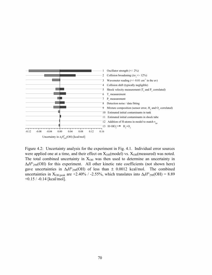
70

-0.12 -0.08 -0.04 0.00 0.04 0.08 0.12 0.16

1 Oscillator strength (+/- 2%)

2 Collision broadening (∆νc+/- 12%)

3 Wavemeter reading (+/- 0.01 cm-1 in the uv)

4 Collision shift (typically negligible)

5 Shock velocity measurement (T5 and P

5 correlated)

6 T1 measurement

7 P1 measurement

8 Detection noise / data fitting

9 Mixture composition (sensor error, H2 and O

2 correlated)

10 Estimated initial contaminants in tank

11 Estimated initial contaminants in shock tube

12 Addition of H-atoms in model to match τign

13 H+HO2 H

2+O

2

Uncertainty in ∆fHo298(OH) [kcal/mol]

Figure 4.2: Uncertainty analysis for the experiment in Fig. 4.1. Individual error sources were applied one at a time, and their effect on ΧOH(model) vs. ΧOH(measured) was noted. The total combined uncertainty in ΧOH was then used to determine an uncertainty in ∆fH°298(OH) for this experiment. All other kinetic rate coefficients (not shown here) gave uncertainties in ∆fH°298(OH) of less than ± 0.0012 kcal/mol. The combined uncertainties in ΧOH,peak are +2.40% / -2.55%, which translates into ∆fH°298(OH) = 8.89 +0.15 / -0.14 [kcal/mol].

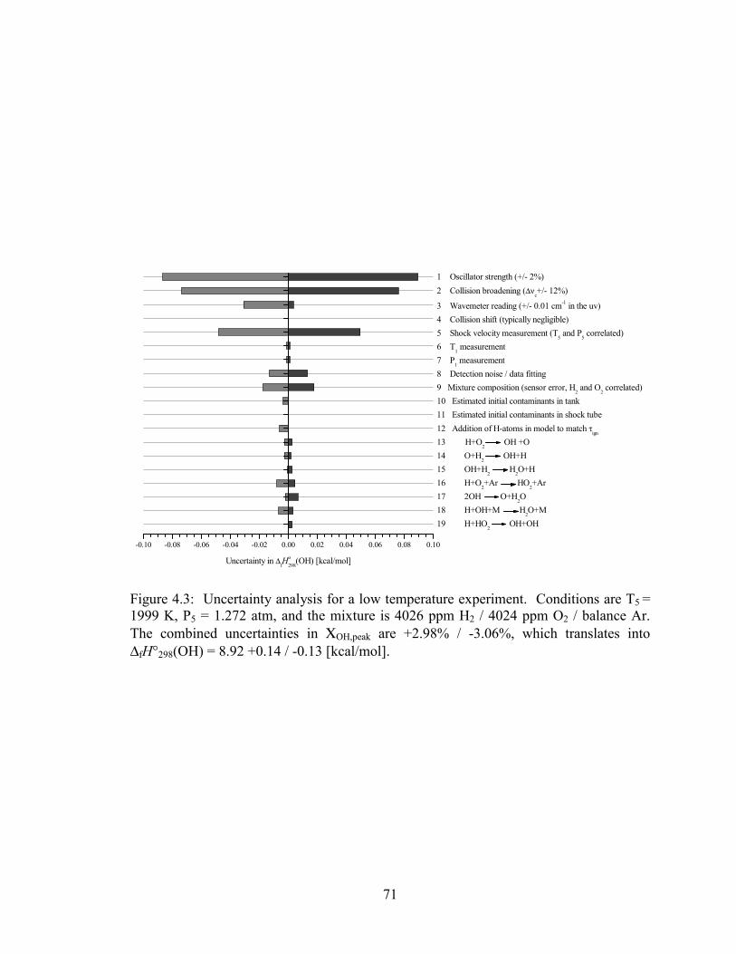
71

-0.10 -0.08 -0.06 -0.04 -0.02 0.00 0.02 0.04 0.06 0.08 0.10

1 Oscillator strength (+/- 2%)

2 Collision broadening (∆νc+/- 12%)

3 Wavemeter reading (+/- 0.01 cm-1 in the uv)

4 Collision shift (typically negligible)

5 Shock velocity measurement (T5 and P

5 correlated)

6 T1 measurement

7 P1 measurement

8 Detection noise / data fitting

9 Mixture composition (sensor error, H2 and O

2 correlated)

10 Estimated initial contaminants in tank

11 Estimated initial contaminants in shock tube

12 Addition of H-atoms in model to match τign

13 H+O2 OH +O

14 O+H2 OH+H

15 OH+H2 H

2O+H

16 H+O2+Ar HO

2+Ar

17 2OH O+H2O

18 H+OH+M H2O+M

19 H+HO2 OH+OH

Uncertainty in ∆fHo

298(OH) [kcal/mol]

Figure 4.3: Uncertainty analysis for a low temperature experiment. Conditions are T5 = 1999 K, P5 = 1.272 atm, and the mixture is 4026 ppm H2 / 4024 ppm O2 / balance Ar. The combined uncertainties in ΧOH,peak are +2.98% / -3.06%, which translates into ∆fH°298(OH) = 8.92 +0.14 / -0.13 [kcal/mol].

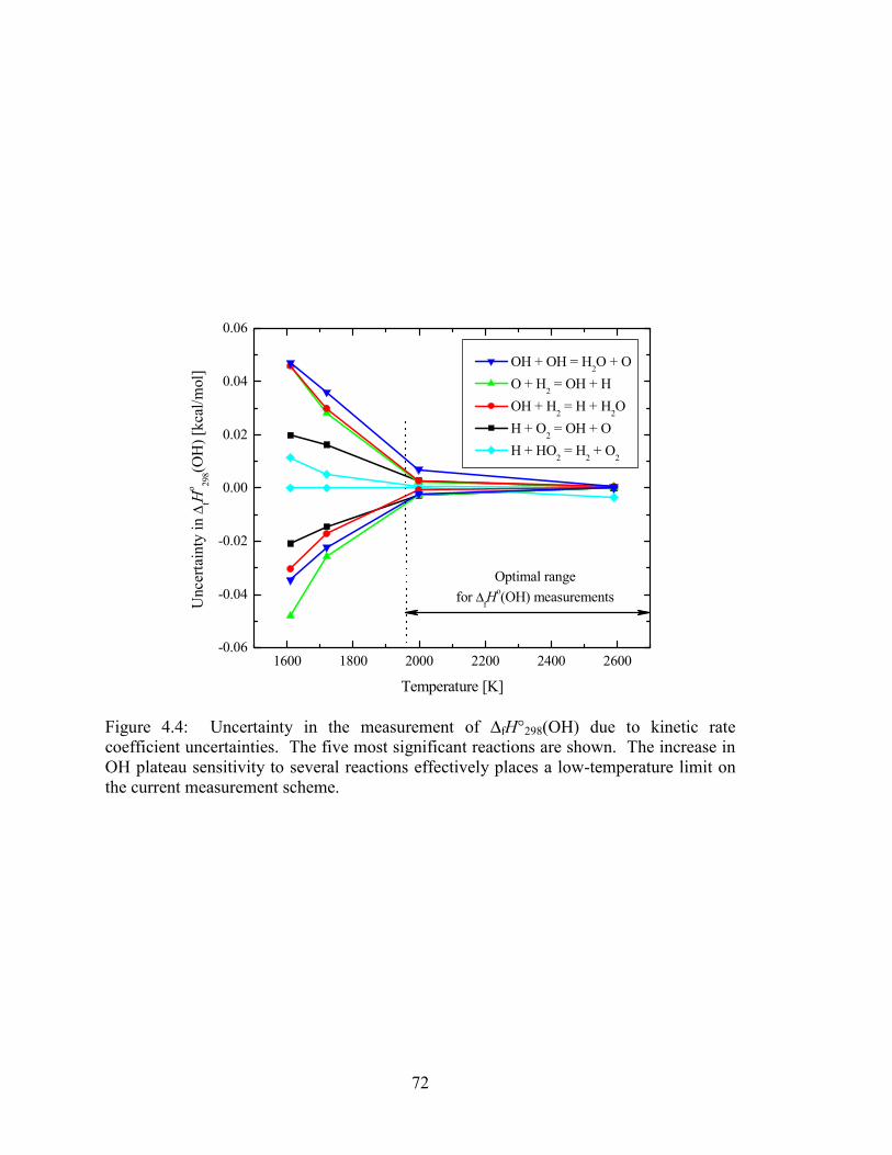
72

1600 1800 2000 2200 2400 2600-0.06

-0.04

-0.02

0.00

0.02

0.04

0.06

Unc

erta

inty

in ∆

fHo 29

8(OH

) [kc

al/m

ol]

Temperature [K]

OH + OH = H2O + O O + H2 = OH + H OH + H2 = H + H2O H + O2 = OH + O H + HO2 = H2 + O2

Optimal rangefor ∆fH

o(OH) measurements

Figure 4.4: Uncertainty in the measurement of ∆fH°298(OH) due to kinetic rate coefficient uncertainties. The five most significant reactions are shown. The increase in OH plateau sensitivity to several reactions effectively places a low-temperature limit on the current measurement scheme.

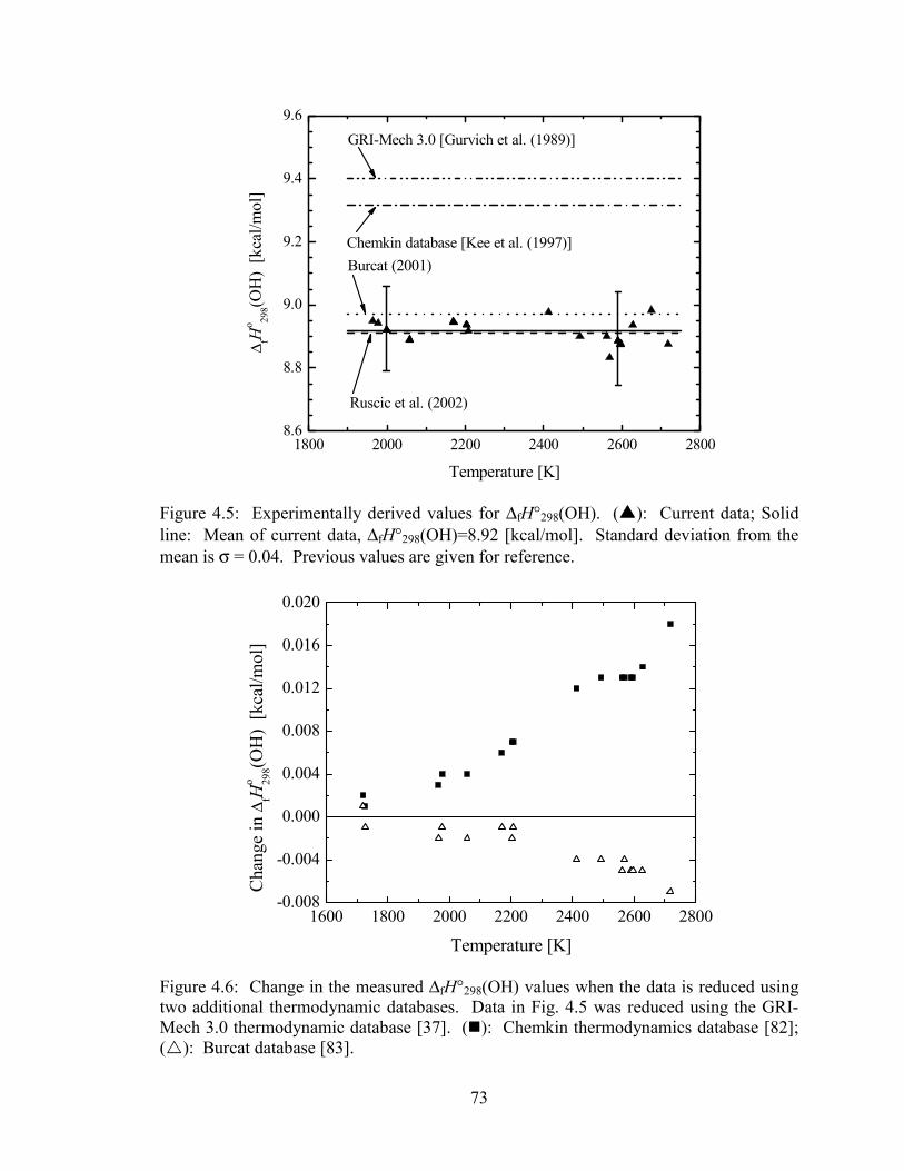
73

1800 2000 2200 2400 2600 28008.6

8.8

9.0

9.2

9.4

9.6

∆ fHo 29

8(OH

) [k

cal/m

ol]

Temperature [K]

GRI-Mech 3.0 [Gurvich et al. (1989)]

Chemkin database [Kee et al. (1997)]Burcat (2001)

Ruscic et al. (2002)

Figure 4.5: Experimentally derived values for ∆fH°298(OH). (�): Current data; Solid line: Mean of current data, ∆fH°298(OH)=8.92 [kcal/mol]. Standard deviation from the mean is σ = 0.04. Previous values are given for reference.

1600 1800 2000 2200 2400 2600 2800-0.008

-0.004

0.000

0.004

0.008

0.012

0.016

0.020

Cha

nge

in ∆

fHo 29

8(OH

) [k

cal/m

ol]

Temperature [K]

Figure 4.6: Change in the measured ∆fH°298(OH) values when the data is reduced using two additional thermodynamic databases. Data in Fig. 4.5 was reduced using the GRI-Mech 3.0 thermodynamic database [37]. (�): Chemkin thermodynamics database [82]; (�): Burcat database [83].

75

Chapter 5: Conclusions

5.1 Summary of results

5.1.1 CH3 + O2 → products

The work presented in this thesis represents a unique experimental determination

of the rate coefficient for the reaction CH3+O2→products and its individual high-

temperature product channels:

CH3+O2→CH3O+O (1a)

CH3+O2→CH2O+OH (1b)

Through a combination of diagnostics which take advantage of the commonality and

difference in the product channels and their subsequent reaction pathways, temperature-

dependent reaction rate coefficient expressions for each individual reaction could be

determined. This determination was completely experimental, with no a priori

assumptions required or imposed in order to resolve the product channel contributions.

The overall rate coefficient, k1, was first determined in a series of experiments

designed to be sensitive to k1 but insensitive to the branching ratio, α, and secondary

reactions. With k1 established, a series of experiments was conducted with almost

exclusive sensitivity to k1a. Brief iteration between the two series of experiments resulted

in the following rate coefficient expressions for the temperature range 1590 to 2430 K:

k1a = 6.08x107 T1.54exp(-14005/T) cm3mol-1s-1

k1b = 68.6 T2.86exp(-4916/T) cm3mol-1s-1

For the measurement of k1a, the average estimated uncertainty over this temperature

range is ± 33%, with a standard error of fit of 11.7%. The k1 measurements have an

average estimated uncertainty of ± 22% with a standard error of fit of 12.9%.

Propagation of these uncertainties through to k1b results in a fairly conservative estimate

of ± 27% at low temperatures and ± 41% at high temperatures for that channel.

76

The present measurements of k1 compare well with one other recent shock tube

measurement [24] and an ab initio theoretical calculation [1]. In particular, the

conclusions of this work lend support to the theoretical calculations with only small

changes recommended in the energetics of the potential energy surface. While the rate

for k1a agrees with two other recent shock tube studies [12,16], the final rate expressions

presented here clearly disagree with the recent conclusions of Michael et al. [16] which

suggest that k1b is unimportant. Rather, as has been concluded by most investigations and

was presumed by the earliest studies of methane oxidation, channel (1b) is found to be

the dominant channel up to high temperatures - in this study at least to 2700 K.

5.1.2 Heat of formation of OH

A unique, high-temperature measurement of the standard heat of formation of the

OH radical, ∆fH°298(OH), has been performed using a shock tube. Equimolar mixtures of

H2 and O2 in an Ar bath gas produced controlled concentrations of OH in the post-

ignition partial equilibrium state behind the reflected shock wave. The OH plateau

concentrations were sensitive primarily to thermochemical parameters, of which the heat

of formation of OH was both the most sensitive and most uncertain parameter. By

design, the OH plateau was very insensitive to kinetic rate coefficients.

High-accuracy measurements of OH using laser absorption were performed. The

spectroscopy and calculation of OH absorption coefficients were carefully reviewed and

updated in an effort to minimize uncertainties. Measurements were compared to and fit

by model predictions both from the analytical solution of the partial equilibrium state and

from full kinetic models.

A series of experiments over the temperature range 1964 K to 2718 K yielded a

temperature-independent average value of the heat of formation of ∆fH°298(OH) = 8.92 ±

0.16 kcal/mol, with a standard deviation in the measurement of σ = 0.04 kcal/mol. The

temperature independence of the measured values is a validation of the spectroscopic

parameters and experimental methods used in this work. The current study agrees very

well with the extensive theoretical and experimental room-temperature study of Ruscic et

al. [30] and the thermochemical cycle calculations of Joens [35], and corroborates the

77

suggestion that the previously accepted values, ∆fH°298(OH) = 9.32-9.4 kcal/mol, are in

error.

5.1.3 Publications

The work detailed in this thesis has been published in the following papers:

J.T. Herbon, R.K. Hanson, C.T. Bowman, and D.M. Golden, “The reaction of CH3 + O2:

Experimental determination of the rate coefficients for the product channels at

high temperatures,” accepted for presentation at the 30th International Symposium

on Combustion and publication in the Proceedings of the Combustion Institute 30

(2004).

J.T. Herbon, R.K. Hanson, D.M. Golden, and C.T. Bowman, “A Shock Tube Study of the

Enthalpy of Formation of OH,” Proceedings of the Combustion Institute 29,

1201-1208 (2002).

J. T. Herbon and R. K. Hanson, “Measurements of Collision-Shift in Absorption Transi-

tions of the OH A-X (0,0) Band Using a Shock Tube,” submitted to JQSRT

(2004).

5.2 Recommendations for future work: Facilities and

diagnostics Future ultra-low concentration, ultra-lean experiments are limited by two primary

issues: the presence of low-concentration impurity species in the gas handling system

and/or shock tube, and the lower limit of OH detection caused by the presence of beam

steering and other shock tube- and flow-related perturbations on the diagnostic laser

beam.

5.2.1 Facilities improvement and impurity reduction

The presence and effects of impurities in the measurements of CH3+O2→products

was an unfortunate but characterizable problem. The significance of the impurities was

78

particularly enhanced in these experiments due to the combination of 1) the desired ultra-

low concentrations of CH3I, meaning that any detectible level of impurity immediately

became a significant fraction of the reactant concentration, and 2) the high mole fractions

of O2, which reacted very readily with the minute levels of impurity species. The

existence of the impurities had several consequences. The effects could be fairly well-

characterized through the measurements of OH and O-atoms in mixtures without CH3I;

however, because the exact identity and character of the impurity species was unknown,

their presence must necessarily increase the uncertainty in the true mixture composition

and therefore the final rate coefficients. Consequently, CH3I concentrations in the

reaction mixtures were kept high enough such that the assumed impurity species

surrogate, typically CH3, was a small fraction of the known reactant concentrations. As

improved isolation of the title reactions could have been achieved with lower CH3I

concentrations and lower CH3I/O2 ratios, the relatively high lower-limit of CH3I

prevented ideal experimental design.

The impurity effect created extra work in that each new mixture concentration

(with different levels of O2) was characterized in a separate sense of experiments,

essentially doubling the number of mixtures, experiments, and the amount of data

reduction required for each data set.

The impurities also affected the calibration of the O-atom ARAS diagnostic.

Most previous investigators have calibrated ARAS diagnostics using the plateau O-atom

concentrations produced from completely dissociated N2O in very low concentration (~1-

5ppm) experiments. In the current work, low-concentration O-atom measurements were

quite obviously affected, as the O-atom concentration never reached the plateau but

rather peaked prematurely and decayed as the O-atoms reacted with the impurity. This

issue forced a new calibration method, whereby higher concentrations were utilized and

the well-studied N2O decomposition rate was used to model the O-atom time-history for

comparison to the experiments. While the new calibration method enabled a large range

of concentrations to be modeled in relatively few experiments, sensitivity to uncertainty

in the kinetic decomposition rate increased the uncertainty in the final O-atom calibration.

Further improvement to the gas handling, mixing, and shock tube facilities is

recommended. The most likely remaining source of much of the impurities is the mixing

79

cylinder itself, based on the observation that impurity effects tend to increase with

mixture residence time in the cylinder. The present mixing cylinder is constructed of an

electrolyzed stainless steel body with a machined aluminum base, sealed by a large O-

ring, and the mixing vanes which appear to be formed of brass. There are many crevices

and some rough surfaces in which low-volatility species may be trapped or adsorbed,

only to slowly diffuse into the gas mixture as it resides in the cylinder. An improved

mixing cylinder might be constructed of a seamless stainless steel cylinder, with or

without mixing vanes. Diffusive mixing or creative gas porting to enhance turbulent

mixing during the fill might replace the extra surface area and complexity of the mixing

vanes. Another option used in many shock tube laboratories is large glass bulbs,

typically several in order to have sufficient volume for a set of experiments.

Improvement of the vacuum capabilities of the mixing cylinder and gas handling

system should also reduce impurity effects, as evidenced by the significant improvements

gained with the redesign and assembly of the existing turbomolecular vacuum pump

system (see Section 3.3.3). Vacuum capability will automatically be enhanced with a

superior leak-free mixing cylinder, and additional effort may find other sources of leaks

in the gas handling system. Calculations should be performed to determine the limiting

orifices in the vacuum system, as the valves and connections, not the pump itself, are the

limiting factor in the pumping-speed capabilities.

Impurity effects, although smaller, were also observed independent of the gas

mixing system in pure O2 experiments with the source gas connected directly to a shock

tube port. These impurities have several potential sources, including crevices between

shock tube sections, O-ring seals, and adsorbed species on the shock tube walls. Once

again, a lower ultimate vacuum pressure is recommended as a means to help reduce

effects of the impurities. Vacuum pressure can be enhanced by further leak detection and

removal, addition of another pump or relocation of the pumping system nearer to the

endwall and test ports (it is currently located in the center of the driven section), and

improvement of effective pumping speeds through redesign of vacuum pathways and

larger pumps if dictated. Previous researchers have also attained improvement in

impurity levels through the use of non-hydrocarbon cleaning solvents, greaseless or metal

seals for ports and shock tube sections, aluminum diaphragms, and bake-out processes.

80

The latter two were tested in this work with little improvement, although the bake-out

was limited to lower temperatures than have been used by other researchers.

5.2.2 Diagnostics improvements

Improved kinetic isolation of reactions of interest can sometimes be obtained by

using very low-concentration reactant mixtures. With that benefit, however, comes the

challenge of measuring ever-decreasing absorption signals. After the aforementioned

impurity issues are resolved, or in cases where they are not important, low reactant-

concentration experimental schemes are eventually limited by the signal-to-noise or

detection limitations of the diagnostics. Several potential improvements to the OH laser

absorption diagnostic are discussed here.

The first, easiest, and most certain variation which would improve OH absorption

signals would be to use a stronger absorption transition within the A-X(0-0) band. In the

current laser setup, a temperature-tuned AD*A crystal is utilized for the intracavity

frequency doubling process. The range of attainable phasematched frequencies is limited

by the temperature-tuning range of the crystal, in this case 25 to 100 C. Within this

tuning range, the strongest absorption transition at shock tube temperatures is the Q1(3)

transition at 308.24nm. The Q1(3) Einstein A-factor is 2x larger than that for the R1(5)

transition, and the line center absorption coefficient is 2x higher at 1500K and 70%

higher at 2500K. It is a fairly well-isolated line and thus has only minor influence from

adjacent lineshapes (although the Q21(3) lineshape is nearby and a full spectral

calculation should always be performed). The collision-broadening and collision-shift

coefficients have been characterized for this transition in Appendix B, with relatively

high precision and accuracy due to its high intensity and reasonable isolation from

adjacent transitions. For reference, the broadening parameter is almost identical to that

for R1(5), while the shift parameter is somewhat smaller. Even higher absorption

coefficients could be attained with other transitions in the Q1 and Q2 rotational branches;

however this would require a different frequency doubling crystal (potentially angle-

tuned rather than temperature-tuned phasematching) and lineshape parameter

characterization experiments for these new transitions. The relative benefit of these

slightly stronger transitions in the Q1 and Q2 branches is most likely not worth the

81

increased difficulty of angle-tuning an intracavity doubling crystal (adjustments to

optimize the phasematching angle simultaneously affect the cavity alignment, which does

not happen in temperature-tuned crystals).

Another avenue to improved signal-to-noise measurements may be through the

use of multiple passes of the laser beam. Multi-passing a laser beam in shock tube

experiments has been attempted in the past with success [86], as have multi-pass lamp

absorption diagnostics [87,88]. Multiple passes of the laser beam have the obvious

benefit of enhancing the absorbance by increasing the path length, but questions remain

as to its real potential for improving signal-to-noise. The primary question pertains to the

location of origin of the perturbations to the beam intensity and/or direction of

propagation which are causing the noise in the first place. For example, if the beam is

being deflected in a random manner by gasdynamic effects in the post-shock region, that

deflection may cause one or more consequences. The beam may encounter locations of

poorer transmission in the shock tube windows or any downstream optic (e.g. dust

specks, scratches, etc.). Alternatively, the beam may be moving off of the uniform

sensitive area of the photodiode. Another type of beam perturbation can occur in very

high pressure shock tube experiments, where photoelastic effects in the shock tube

windows have caused polarization scrambling and subsequent attenuation of the beam by

downstream optical surfaces [41].

Depending on the origin and character of the perturbation of the beam, a multiple-

passing scheme may or may not yield improved detection limits. If each successive pass

of the beam through the post-shock gases and/or windows yields an additive intensity

perturbation on the beam, no additional beam passes will yield any improvement and

may, in fact, prove to be detrimental to the signal. If the additive perturbation is in the

propagation direction of the beam, the multi-passing beam alignment must be relatively

tolerant of beam steering and adequate collection optics and sufficient optical apertures

must be capable of channeling the roving output beam into the detection system.

Initial attempts at multi-pass absorption were performed in the present work, with

somewhat limited improvement in signal-to-noise. Here, the beam was passed 3 or 5

times in a vertical zig-zag pattern between two external mirrors. In these trials, signal-to-

noise improved by ~2x with either 3 or 5 passes. The limited improvement may have

82

been an artifact of the increasing beam diameter combined with the limited exit aperture

required to achieve the multiple reflections. (It should also be noted that at the time of

these trials, the detectors had suffered as-yet-undetected damage from high intensity UV

beams, creating a very non-uniform sensitive area.)

Two potential multi-pass schemes may yield drastically improved signal-to-noise,

depending, of course, on their specific design and the characteristics and origin of the

beam perturbations. One scheme involves a multi-pass cell utilizing curved mirrors

either external to the shock tube windows or in place of the shock tube windows

themselves. This type of system, developed by Baer et al. [89] for static cell

measurements, yields extremely long path lengths and, depending on its tolerance to

beam steering, may or may not yield strong improvements in signal-to-noise. Other

designs with fewer passes are certainly possible. A potential limitation of this type of cell

is the spatial requirements of the beam pattern, which would necessarily limit the time

resolution of the system due to the shock transit time across the multiple beams. The

beam pattern may be able to be manipulated, however, such that it is not much wider than

one beam diameter in the direction of the shock tube axis. This multi-pass detection

scheme, called integrated cavity output spectroscopy (ICOS) [89], is currently being

investigated in our laboratory.

A second potential scheme is similar to the ICOS design, except that the beam

would be propagated perpendicularly through the center of the windows/mirrors in a

single overlapping path. If the mirrors were placed external to the shock tube windows

(which would most likely be the case), the windows would be given an anti-reflection

coating to reduce losses. The benefits to this scheme over the ICOS design is the better

time resolution capability due to the spatially-narrow absorption beam path, and perhaps

less sensitivity to beam steering due to the non-prescribed beam path. It is unclear at this

time whether such a scheme will be more or less tolerable to beam deflections during the

multiple passes. The dangers in this scheme are that any potential optical resonance

between the perpendicular surfaces in the cavity, particularly the high-reflectivity cavity

mirrors, must be destroyed or otherwise overcome, as the window-flexing, vibrations, or

other optical path perturbations will potentially create moments of resonant behavior and

spurious high optical transmission through the cavity. One method to overcome the

83

resonance effects may be to install a constantly vibrating cavity optic, like a mirror

mounted to a piezoelectric transducer with a white-noise or constant high-frequency

driver signal, which would result in a consistent level of on-and off-resonance output that

would blur out any spurious resonance effects

A third technique for drastically improving signal-to-noise in shock tube

experiments is UV frequency modulation (FM) absorption spectroscopy. This technique

has already proven highly successful in shock tube research for the species 1CH2 [90],

NH2 [91,92], and HCO [64], all of which have absorption transitions in the visible

wavelengths. These examples of FM spectroscopy have typically resulted in detectivity

improvements of factors of 10-20. Frequency modulation spectroscopy has the distinct

advantage of canceling out flow- and shock tube-related perturbation effects on the beam,

as the system is only sensitive to differential absorption and not common-mode effects on

the frequency sidebands. Development of a UV FM technique for OH was initially

considered for the work on CH3+O2→products, but was set aside in favor of other more

pressing projects. In the end, its potential enhanced sensitivity was deemed unnecessary

and in fact would have been even less important in light of the impurity limitations on the

low-concentration mixtures. Although its sensitivity was not required, advantage could

have been gained from lower noise and smoother data traces.

The equipment has been acquired and an initial design and troubleshooting of the

setup was accomplished. For this work, a specially made 1GHz phase modulator was

built by Quantum Technologies, Inc. using (5) 1x1x18 mm β-barium-borate (BBO)

crystals. In the initial work with this setup some phase modulation was evident, but there

was also evidence of non-ideal polarization behavior in the phase modulator resulting in

an elliptically-polarized output beam being created from a linearly polarized input beam.

This issue must be resolved in order for the system to function properly.

Initial characterization and calibration of the FM system will be aided by the use

of the OH reference cell, described in Chapter 2, which can create steady OH

concentrations for long periods of time. An additional benefit in our laboratory is the

ability to rapidly-scan the UV laser wavelength across the whole transition lineshape and

well into the wings, and to do so multiple times in a given shock tube experiment. This

capability would enable facile evaluation of the FM lineshape at shock tube conditions,

84

rather than multiple experiments to map out the lineshape as has been done in previous

work [92]. Well-known OH concentrations are easy to produce using the partial

equilibrium plateaus in H2/O2 mixtures, and detailed lineshape information for previously

characterized and isolated lines like the R1(5) and Q1(3) transitions will provide further

understanding of the system calibration and expected FM absorption coefficient.

5.3 Recommendations for future work: Kinetics One primary goal of the present work on CH3+O2→products was to design and

execute experiments which were as insensitive as possible to secondary reaction rates.

This goal was achieved in part through the use of ultra-lean, ultra-low-concentration

mixtures. For the measurement of k1, fitting the normalized OH rise time desensitized

the k1 measurement to any uncertainties in the secondary reactions that control the OH

peak concentration. In the O-atom measurements, the data fit was limited to the initial

portion of the species concentration time-histories where kinetic isolation was

maintained.

While only the normalized traces were used for the determination of k1, these

measurements did produce quantitative OH peak concentrations which can be compared

to model calculations. In general, the measured and calculated OH peaks did not agree

with one another, and the mismatch exhibited smooth and non-monotonic temperature

dependence as given in Fig. 3.13. Several reactions display high sensitivities at the OH

peak, as given in Fig. 3.14, and the next challenge is to deconvolve which secondary

reaction rates are in error, by what magnitude, and the temperature dependence of their

error.

Of the sensitive reactions which control the OH peak, some have relatively well-

known rate coefficients, while others have very sparse or highly uncertain data at shock

tube temperatures and therefore should be studied further. Table 3.3 provides a list of

reactions and their estimated uncertainties, some of which also feature strongly in Fig.

3.14. These uncertainties were assessed based on the most recent evaluation of Baulch et

al. [62], in comparison with the actual rates used in GRI-Mech 3.0.

85

Similarly, the long-time O-atom concentrations are sensitive to secondary

reactions with relatively high uncertainties. The most important secondary reactions in

the O-atom measurements have been included in Table 3.3.

The improvement in secondary reaction rate coefficients can be approached on

two fronts. First, dedicated high-sensitivity well-isolated kinetics experiments might be

designed to accurately measure some secondary rates and decrease their estimated

uncertainties. Reactions with outstanding uncertainties and limited measurements at

shock tube temperatures include OH+HO2 →H2O+O2, CH2O+O2 →HO2+HCO, and

O+CH2O→OH+HCO. The state of knowledge on these reactions was discussed in

Section 3.5.4.

A second and perhaps less pragmatic approach to investigating the secondary

chemistry is to use the quantitative data from the present OH and O-atom measurements

in a constrained optimization scheme. This type of mechanism optimization has been

discussed in detail by Frenklach et al. [93], and has been used extensively in the

optimization of the GRI-Mech series of natural gas combustion mechanisms [37].

Optimization is an ideal procedure for fitting several sets of data with several variable

reaction rates. In the present circumstances, the combination of both quantitative OH and

O-atom data, with their distinct reaction sensitivities over a range of mixtures and shock

conditions, will lend extra information to the optimization, in addition to the normalized

OH rise time.

One last recommendation pertains to the development and evolution of optimized

mechanisms such as GRI-Mech 3.0. In the present work on CH3+O2→products, the rates

for k1a and k1b were adjusted to fit the present set of measurements alone, while ignoring

the larger set of target data to which the original mechanism was optimized. This is

somewhat antithetical to the true intention of the optimization process, which is to build a

mechanism that takes into account a wide variety of data and is optimized to best-fit the

whole collection of evaluated experimental targets. While the author believes that the

present experiments were well-designed and carefully executed, the resulting rate

coefficients, where different from the starting mechanism, will impact the quality of the

mechanism’s agreement with the specific GRI-Mech targets which are also sensitive to

the adjusted rate coefficients (e.g. CH4 ignition time targets similar to Fig. 1.1). The

86

proper procedure for improving the whole chemical mechanism would be to perform a

full re-optimization after making the following changes. First, the mechanism should

include the present OH rise time data, O-atom concentration data, and OH peak

concentration data as new targets. The new rates for k1a and k1b should be retained in the

starting mechanism. Appropriate uncertainty limits, as determined in Chapter 3, should

be enforced as the constraints on k1a and k1 (and therefore k1b). Finally, reactions for

which new experimental data has been published should be re-evaluated and updated in

the new starting mechanism. Some of these reactions are listed in Table 3.4.

A new, full optimization of the GRI-Mech mechanism is a large undertaking and

is beyond the scope of this thesis. Such an optimization run, including the new starting

rates, targets, and constraints, will most likely result in changes to other reactions

sensitive to the new targets and some original targets which share sensitivities with

reactions (1a) and (1b). This is the expected and desired outcome. As this is a

constrained optimization, provided that the constraints on all reaction rate coefficients are

appropriately assigned, the optimization should only result in a superior overall

combustion mechanism. Such an improved combustion mechanism, finally, is the true

and anticipated goal of the experimental work presented in this thesis.

87

Appendix A: Calculation of OH spectral absorption coefficients

A.1 Introduction Chemical kinetics research often involves measurements of species concentration

or mole fraction as a function of time. Whether one is interested in sensitive

measurements of individual fundamental reaction rate coefficients, or species profiles for

use in evaluating a chemical reaction mechanism, accuracy and precision in the species

concentration data is typically a requirement. Uncertainties enter into measurements in

several forms, including both random and systematic experimental errors and noise, and

uncertainties in calculated parameters such as spectroscopic line strengths and line

shapes. In the case of absorption, an experiment involves measuring the fractional

absorption and is described (for a uniform path length L) by the Beer-Lambert law:

( )PXLk I

I transν−=== exp n)(Absorptio -1 ion)(Transmiss

0

(A.1)

Data reduction of measured absorption to obtain mole fraction, Χ, is therefore dependent

on pressure, pathlength, and the spectral absorption coefficient kν – which is itself a

function of temperature, pressure, absorption frequency, and collision partners.

Estimation of measurement uncertainties must take into account the individual

uncertainties in each of these parameters.

This appendix will discuss calculation of the absorption coefficient, kν.

Calculation of kν includes two parts: the integrated absorption intensity, Slu, and the line

shape factor φ(ν):

( )νφluν Sk = (A.2)

While different forms exist for Slu, the following equation described by Goldman and

Gillis [72] is most frequently and most easily used for narrow-linewidth laser absorption:

88

( ) ( ) ( ) ( )[ ]T-JAQ

TEPN

πcνTS ul

totOHlu /4388.1exp112/4388.1exp

81

2 ν−+′′′−

= (A.3)

Calculation of Slu requires values for the lower-state energy, E”, the Einstein A-

coefficient, Aul (which is related to the oscillator strength of a transition), the transition

frequency, ν, and the total partition function, Qtot. Researchers requiring quantitative

measurements are interested in the accuracies of each of these parameters in Equations

(A.2-A.3), and how they relate either directly or indirectly to an absorption coefficient

uncertainty and therefore potential errors in the measured species concentration.

Experimental prudence demands that such parameters are calculated or controlled to the

highest possible precision and accuracy, so that measurements are dominated only by

random or otherwise uncontrollable uncertainties. A survey of recent spectroscopic data

is given here, and the calculation of the total partition function is described.

A.2 Spectroscopic data Over 40 years have passed since the first extensive publication on the UV bands

of OH by Dieke and Crosswhite [94]. In this time period, numerous researchers have

undertaken studies of the UV, IR, and microwave absorption and emission spectra of OH.

The spectroscopy of OH and a survey of literature on the UV bands of OH up to 1990

have been described previously by Rea [95].

Until 1998, the most complete tabulation of OH line parameters for the A-X(0,0)

band was by Goldman and Gillis [72], who listed transition frequencies, A-coefficients,

lower-state energy levels, and values or formulas for use in calculating the partition

function. Using their methods and data, along with appropriate line shape factors, the

absorption coefficient can be easily calculated for lines with J” up to 40.5. This is the

database on which Rea and other researchers in our laboratory have based OH

concentration measurements in the past. However, over the last 10 years, researchers

have extended the spectroscopic database to include measurements of more spectral lines

in the UV, IR, and microwave regions and, in particular, improved accuracy of spectral

line positions for the (0,0) band. These data permit improved fitting of spectroscopic

constants, yielding increasingly accurate values for energy levels and providing more

precise input parameters for the calculation of rotational transition probabilities.

89

The most recent measurements of the OH A-X(0,0) transition frequencies have

been performed by Stark et al. [73]. Rotational lines up to J” = 30.5 were measured

from Fourier-transform spectra of a hollow-cathode source, with absolute line position

accuracies of ~0.001 cm-1 for the strongest lines. Sets of molecular parameters and

rotational term values (lower-state energy values, E”) were derived from these measured

line positions. These measured transition frequencies are still the most precise data

available today, and should be used as the vacuum line-center frequencies when

calculating and modeling the spectral absorption coefficient.

Luque and Crosley have performed the most recent calculations [75] and

tabulation [77] of absolute transition probabilities for the OH A-X system. These

supercede earlier calculations by Chidsey and Crosley [96] and others. Improvements

and extensions to measured band transition probabilities, as well as new spectral data at

high vibrational levels, have together enabled better calculation of the potential curves

and a more accurate form for the electronic transition moment. This, in turn, has lead to

higher accuracy in the relative, rotational level-dependent transition probabilities.

Relative probabilities are put on an absolute scale using the experimentally-determined

radiation lifetime [76]. Values of Aul in this new work can vary significantly from the

older tabulation of Goldman and Gillis, with differences of 0.5-5% for J ≤ 25 in main

transitions and 5-20% in satellite transitions. For satellite transitions at higher J,

differences can be up to a factor of 2 [74].

Finally, Gillis et al. [74] repeated the tabulation of Goldman and Gillis [72], now

utilizing the line position measurements of Stark et al. [73] and the updated transition

probabilities of Luque and Crosley [77]. They also extended the tabulation beyond the

(0,0) band to include the six strongest bands of the OH A-X system. Once again, their

tabulation includes the Einstein A-coefficients (which are taken exactly from Luque and

Crosley [77]), transition frequencies, and lower-state energy values E”. The frequencies

and E” values were calculated using the molecular constants of Stark et al. [73]. For the

strong, low J”, R1-branch lines of the (0,0) band these calculations agree with the

measurements of Stark et al. to 0.001 cm-1 for ν and better than 2 parts per million for the

E” values. For v” > 0, the E” of Gillis et al. [74] include a vibrational contribution

using the constants of Coxon [97]. It is not clear why they choose to use the constants of

90

Coxon rather than those of Luque and Crosley [75], which are determined from a fit

including higher vibrational levels than that of Coxon. However, for v” = 0,1,2 the

differences between using these two sets of constants is negligible.

In the attempt to calculate accurate integrated linestrengths, Slu, the most recent

parameter values should be used. These would include A-coefficients from Luque and

Crosley [77], E” values from Gillis et al. [74], and the measured transition frequencies of

Stark et al. [73]. Of these parameters, the largest uncertainty arises from the

experimental radiative lifetime of German [76]. This value is required to transform the

calculated relative transition probabilities, which themselves have quite good accuracy,

into absolute values. The reported 3σ uncertainty by German is ± 3% and translates

directly into an uncertainty in the integrated line strength.

A.3 Partition functions The total internal partition function, Qtot, describes the number of ways that the

thermal energy in a group of molecules is divided up among the allowed quantized

energy levels. It enters the calculation of Slu as a part of the Boltzmann fraction,

describing the percentage of all absorbing molecules which exist in a given energy state

at thermal equilibrium. Thus, the partition function directly influences the absorption

coefficient of a particular transition and should be calculated as accurately as possible.

The true partition function, Q(T), is found by summing over all possible energy

levels of a molecule:

( ) ( )/kT-hcEgTQ ii

i exp∑= (A.4)

where Ei is the total energy of the molecule in a given level i, and gi is the degeneracy of

the energy level (i.e., the number of possible states of the molecule which have the same

quantum number assignments and thus the same energy). The total partition function,

Qtot, can be factored into an individual partition function for each type of independent

energy mode. Except at very low temperatures, it is quite accurate to separate the total

energy into electronic energy and a combined vibrational-rotational energy. With

somewhat reduced accuracy, this vibrational-rotational energy can be separated into

vibration and rotation components. The loss of exactness in this separation is due to the

91

centrifugal effects of the rotation on the vibrational modes, and the influence of the

vibrational motion on the rotational moment of inertia [98]. Higher-order terms can be

utilized to compensate both the rotational and vibrational term energy formulas for these

intermodal effects. Therefore, it is reasonable to separate the energies and thus factor the

partition function – requiring one to simply calculate the partition function contributions:

Qtot=QelecQvibQrot.

Various simplifying approximations have been invoked in the past for use in

calculating the different components of the partition function, most likely for ease of

computation and lack of data on high-lying energy states or higher order constants for the

term energy equations. While these approximations allow an estimated value for Qtot to

be quickly calculated, they are often grossly incorrect at one or both ends of the

temperature spectrum. However, with computers and simple programs it is easy to

calculate the full summations for the partition function, using the improved spectral and

energy level information made available over the past 2 decades. It is only sensible to

perform this full calculation to obtain the most accurate value for Qtot.

To understand the improvement in Qtot when a full summation is calculated, the

approximations others have used in the past can be examined. The simplest model for a

diatomic molecule is called the rigid rotor / simple harmonic oscillator (SHO). In this

model, valid only at high temperatures or for small rotational constants (Bv) (i.e., for

many closely-spaced rotational energy states), the rotational partition function Qrot

summation can be approximated by an integral [78], yielding simply:

vhcBkT Qrot = (A.5)

where Bv is the rotational constant of the molecule. Here Bv = B0 = 18.536, using the

rotational constants given by Luque and Crosley [75]. In the rigid rotor approximation,

this rotational constant would apply to all vibrational levels of the molecule.

The vibrational partition function of a simple harmonic oscillator is derived by

assuming that the energy difference between adjacent vibrational levels is constant. In

this case, the full sum in Equation (A.4) can be reduced to the form:

( ) ( )( )( )[ ]/kT-hcω-

/kT-hcGTQe

vib exp10exp= (A.6)

92

If the energy is referenced to the v = 0 state, this form is:

( ) ( )[ ]/kT-hcω-TQ

evib exp1

1=′ (A.7)

The simple harmonic oscillator approximation works fine at low temperatures, where

only the first couple of vibrational states have considerable population. However, at

higher temperatures the upper vibrational states begin to be populated. As these states

are closer together than are the lower states, the large assumed spacing of the harmonic

oscillator will give an erroneously low partition sum.

The electronic partition function component can be accounted for in a couple of

different ways. An approximate method involves calculating the electronic partition

function and rotational partition function separately. In the X2Π state of OH, each set of

energy levels with the same quantum number N is actually made up of four spin-split,

lambda-doubled energy states. Because it is an intermediate Hund’s case (a) and (b), the

spin-splitting starts off quite large at low N values (~100 cm-1), but approaches zero at

higher N. An approximation to a full summation can be made by assuming that these

four spin-split, lambda-doubled states represent a simple degeneracy in the electronic

partition function. The electronic partition function Qelec is then typically written as:

( )( )∑ −=n

eeelec /kTnhcTg Q exp (A.8)

The degeneracy, ge, would be 4.0. Due to the first excited state of OH having Te =

32,684 cm-1, all the exponential terms except for the ground state (Te = 0) drop out at

typical combustion temperatures, leaving Qelec = 4.0. The rotational partition function

would then ignore this four-way splitting, either by using the rigid rotor approximation or

summing the energy states over all quantum numbers N – assuming one state for each N

at the average energy of all states with that same quantum number. At higher

temperatures, where many upper rotational states are populated, this approximation of

Qelec = 4.0 is fairly accurate. Because the spin-splitting of the upper rotational states is

approaching zero, the assumption that all states with quantum number N have the same

energy is a decent approximation. However, at low temperatures, the difference in

energy between states having the same N is significant. When only relatively few states

93

are populated, their correct energy values must be used to obtain an accurate partition

sum.

As long as correct energy level information is available, the most accurate

calculation of the combined electronic/rotation partition function is a full summation over

sufficient energy states such that further addition of more terms adds negligibly to the

partition function. In this case, each of the four spin-split, lambda-doubled states is an

individual term in the summation, and the only degeneracy is the (2J+1) associated with

the number of possible directions of the angular momentum vector. This is the procedure

adopted by Goldman and Gillis [72] for their table of QR ≡ QelecQrot, and it is the preferred

method for obtaining the correct partition function at any temperature. One must always

be cautious that the summation is carried out far enough for the given temperature – i.e.

the summation should converge and additional terms should add effectively nothing. The

table in [72] is based on a summation up to J” = 40.5, and values are given for

temperatures up to 6000 K. Researchers in our laboratory have used these data, fit

appropriate portions of it to a polynomial, and used this fit as a means to interpolate QR to

other temperatures not given in the table with errors of less than 0.1%. For example, a fit

by Rea of the values from 1000-4000 K yielded the following polynomial fit [95] (note

that his thesis contains a sign error, and the last term should be negative): 31126 102404210545491148670109885 T.-T.T..-Q --

R ××++= (A.9)

The most recent tabulations of energy levels [99], based on molecular constants from fits

to the spectral measurements of Stark et al., are also listed up to J” = 40.5. The new

level tabulations yield QR values which agree with Goldman and Gillis to within 0.01%

up to 6000 K. As noted earlier, the summation must be carried out far enough that

further terms add negligibly to the partition function. This can be checked by adding

terms for J” = 41.5-50.5 from a paper by Melen et al. [100]. Adding these terms changes

QR by only +0.1% at 6000 K; and we can conclude that the tables in Goldman and Gillis

are sufficient for temperatures up to 6000 K. However, as the temperature increases

beyond 6000 K these additional energy terms must be included in the sum for the sake of

accuracy. Comparing QR from Equation (A.9) to the full summation from J” = 0.5-50.5,

the polynomial equation agrees with the full summation to within 0.01% from 1000-4000

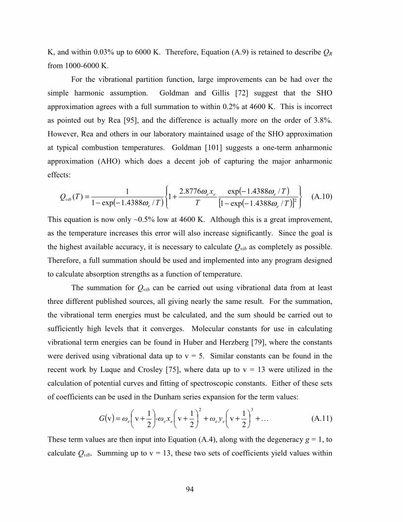
94

K, and within 0.03% up to 6000 K. Therefore, Equation (A.9) is retained to describe QR

from 1000-6000 K.

For the vibrational partition function, large improvements can be had over the

simple harmonic assumption. Goldman and Gillis [72] suggest that the SHO

approximation agrees with a full summation to within 0.2% at 4600 K. This is incorrect

as pointed out by Rea [95], and the difference is actually more on the order of 3.8%.

However, Rea and others in our laboratory maintained usage of the SHO approximation

at typical combustion temperatures. Goldman [101] suggests a one-term anharmonic

approximation (AHO) which does a decent job of capturing the major anharmonic

effects:

( )( )( )[ ]

−−−

+−−

= 2/4388.1exp1/4388.1exp8776.2

1/4388.1exp1

1)(T

TT

xT

TQe

eee

evib ω

ωωω

(A.10)

This equation is now only ~0.5% low at 4600 K. Although this is a great improvement,

as the temperature increases this error will also increase significantly. Since the goal is

the highest available accuracy, it is necessary to calculate Qvib as completely as possible.

Therefore, a full summation should be used and implemented into any program designed

to calculate absorption strengths as a function of temperature.

The summation for Qvib can be carried out using vibrational data from at least

three different published sources, all giving nearly the same result. For the summation,

the vibrational term energies must be calculated, and the sum should be carried out to

sufficiently high levels that it converges. Molecular constants for use in calculating

vibrational term energies can be found in Huber and Herzberg [79], where the constants

were derived using vibrational data up to v = 5. Similar constants can be found in the

recent work by Luque and Crosley [75], where data up to v = 13 were utilized in the

calculation of potential curves and fitting of spectroscopic constants. Either of these sets

of coefficients can be used in the Dunham series expansion for the term values:

( ) l+

++

+

+=32

21v

21v

21vv eeeee yωx-ωωG (A.11)

These term values are then input into Equation (A.4), along with the degeneracy g = 1, to

calculate Qvib. Summing up to v = 13, these two sets of coefficients yield values within

95

0.02% of one another at 6000 K. In addition, it should be noted that the terms for v = 12

and v = 13 contribute 0.06% and 0.04%, respectively, to the vibrational partition sum.

A third set of vibrational data is the tabulated term values of Coxon and Foster

[102]. These are given up to v = 10, and a partition sum using these values yields

agreement with the previous calculations to better than 0.1% up to 6000 K.

A.4 Conclusions Table A.1 has been constructed to compare these approximate and full summation

methods for calculating components of the total internal partition function as a function

of temperature. Error in the total partition function, Qtot, from using simple

approximations can be calculated from consideration of the error in the individual

components and remembering that Qtot=QRQvib. Total errors assumed by using the rigid

rotor, simple harmonic oscillator approximations are 3% at 3000K, increasing at both

higher temperatures and up to 10.5% at room temperature. These errors are large and

unnecessary, and only full summations of the partition functions, or mathematical fits to

the full summations, should be used in future calculations of spectral absorption

coefficients.

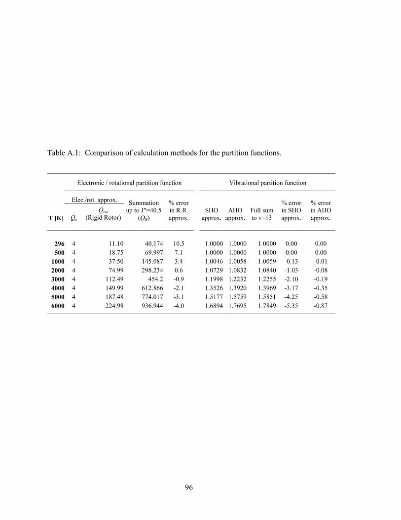
96

Table A.1: Comparison of calculation methods for the partition functions.

Electronic / rotational partition function Vibrational partition function

Elec./rot. approx.

T [K] Qe Qrot

(Rigid Rotor)

Summation up to J"=40.5

(QR)

% error in R.R. approx.

SHO approx.

AHO approx.

Full sum to v=13

% error in SHO approx.

% error in AHO approx.

296 4 11.10 40.174 10.5 1.0000 1.0000 1.0000 0.00 0.00 500 4 18.75 69.997 7.1 1.0000 1.0000 1.0000 0.00 0.00

1000 4 37.50 145.087 3.4 1.0046 1.0058 1.0059 -0.13 -0.01 2000 4 74.99 298.234 0.6 1.0729 1.0832 1.0840 -1.03 -0.08 3000 4 112.49 454.2 -0.9 1.1998 1.2232 1.2255 -2.10 -0.19 4000 4 149.99 612.866 -2.1 1.3526 1.3920 1.3969 -3.17 -0.35 5000 4 187.48 774.017 -3.1 1.5177 1.5759 1.5851 -4.25 -0.58 6000 4 224.98 936.944 -4.0 1.6894 1.7695 1.7849 -5.35 -0.87

97

Appendix B: Measurements of collision shift in the OH A-X(0,0) band

B.1 Introduction

B.1.1 Motivation

Narrow-linewidth lasers have been employed as a diagnostic tool in shock tube

chemical kinetics research for over 20 years. The high signal/noise ratio, species

selectivity, and improved detectivity compared to broadband optical techniques (such as

lamp absorption or emission) make laser absorption and fluorescence attractive for use in

complex reacting flows, where many species are present and often the molecule of

interest exists in concentrations on the order of parts-per-million. Quantitative absorption

measurements using a narrow-linewidth light source require accurate knowledge of the

spectral absorption coefficient, which is simply the product of the integrated line intensity

and the lineshape function: kν = Slu*φ(ν). Calculation of integrated absorption intensities

for OH has been reviewed in Appendix A. The lineshape function, φ(ν), for an individual

spectral line is a function of temperature, pressure, and the species with which the

molecule of interest is interacting. In this appendix, the absorption lineshape of OH will

be explored.

An understanding of the lineshape parameters is critical to accurate laser

measurements, particularly for more advanced diagnostics. Recently workers in our

laboratory and other institutions have developed and applied frequency modulation (FM)

absorption techniques in shock tube research, increasing the sensitivity (decreasing the

lower detection limit) of certain species by over a factor of 10 [64,90-92]. Such

improvements enable significantly lower concentrations to be used in chemical kinetics

98

experiments, thereby providing better isolation of the chemistry of interest and reducing

the influence of secondary reactions. Compared to simple absorption experiments, where

the laser wavelength is often tuned to the peak of a strong transition to attain maximum

absorption signal, FM absorption is performed by tuning the laser wavelength to a

location on the lineshape which has the greatest slope. The frequency modulation

process creates frequency sidebands centered about the carrier frequency. Only the

differential absorption of the sidebands is detected, and any common-mode signal

disturbances such as flow turbulence and beam steering, window effects, vibration, or

laser power fluctuations are cancelled out.

The use and calibration of such an FM technique for OH would especially benefit

from accurate lineshape information, as the FM absorption coefficient (with the laser

tuned to the side of the lineshape) is much more sensitive to the broadening and shift of

the line than is the more commonly used peak absorption coefficient [90]. Figure B.1

illustrates the magnitude of shift expected for OH lineshapes. At these conditions (1500

K, 4 atm), absorption at the lineshape peak may be affected by ~ 7% if the shift is

unaccounted for. On the other hand, initial calculations suggest that the FM absorption

signal could be affected by as much as 25% based on the same magnitude of collision

shift. The need to correctly model the OH lineshape to achieve highly accurate

measurements, both for conventional absorption techniques and especially for FM

techniques, is evident.

B.1.2 Background

The most commonly used lineshape for modeling the absorption transitions of

many molecules is a shifted Voigt profile. This symmetric profile is constructed from a

convolution of the Gaussian lineshape (an effect due to the molecular velocity

distribution), and a Lorentzian lineshape (due to state-perturbing collisions with other

molecules). The shift of the line-center frequency is simply described by ∆νs = ΣδiPi,

where Pi is the partial pressure of the collision partner; and the collision shift coefficient

has the form δi(T) = δi(Tref)*[Tref/T]n cm-1atm-1. Simple kinetic theory of hard-sphere

collisions predicts a value of n = 0.5 for the temperature exponent, while in practice n

typically ranges between 0.5 and 1.

99

The spectroscopic lineshape parameters of the OH radical have been

experimentally researched by several authors. Numerous studies of the collision

broadening over a wide range of transitions and conditions have been undertaken in our

lab and elsewhere [39,103-107]. The collision shift, on the other hand, has not been as

thoroughly examined, and the limited condition space which has been studied is shown in

Fig. B.2. The first measurement by Shirinzadeh et al. [104] was performed for a single

transition, P1(2), in the A-X(0,0) band at room temperature for a variety of collision

partner species. Their work verified the linear pressure-dependence of the shift and

collision width up to one atmosphere. Previous investigators in our laboratory [106]

explored the collision shift and width of the A-X(0,0) R-branch bandhead at high

pressures and determined coefficients appropriate to a single high-temperature point for

this composite absorption spectrum. Finally, Kessler et al. [107] studied broadening and

shift of the A-X(1,0) band of OH in a hydrogen-air flame. Their measurements of

collision shift were limited to 3 transitions and were necessarily performed in a mixture

of collision-partner species in the post-flame gases. These three studies provide a starting

point for estimating collision-shift parameters, but are limited in their information

regarding the dependences on temperature, rotational state, rotational branch, and

collision partner at the high-temperature conditions typical of shock tube kinetics

experiments. Because of the interest in quantitative, high sensitivity measurements of

OH in our laboratory, more complete information regarding the collision shift of the OH

molecule is needed.

The present work includes collision-shift measurements for several transitions in

the A-X(0,0) band for the most common shock tube bath gases, Ar and N2. Particular

focus is on the R1(5) transition, due to its frequent usage in shock tube experiments, and

the P1(1) and P1(2) transitions for the purpose of comparison with the room-temperature

data of Shirinzadeh et al. Trends are observed in the collision shift dependence on

temperature, rotational quantum number (J"), and collision-partner species.

B.2 Experimental details Experiments in this work were performed using the shock tube facility and OH

laser diagnostic described in Chapter 2. Partial equilibrium plateau levels of OH (see

100

Chapter 4 and Appendix E) were produced using equimolar mixtures (0.2% or 0.3%

each) of H2 and O2 in a bath of either Ar or a 50/50 mixture of Ar and N2 gas. All

mixtures were > 99% bath gas.

Post-reflected-shock temperature and pressure are calculated using the initial

conditions and the measured shock velocity. For experiments in Ar, the temperature and

pressure behind the reflected shock wave are calculated assuming chemically frozen and

vibrationally equilibrated gases in both the incident and reflected shock regimes.

However, for experiments in N2/Ar the post-shock gases are initially vibrationally frozen,

and the relatively slow vibrational relaxation is predicted to cause an exponential decay

in the pressure and translational temperature of the gases. To complicate the situation

slightly, in the actual experiments with N2 the pressure at the test section was observed to

increase slowly after passage of the shock wave, most likely due to minor gasdynamic

non-idealities. Therefore, the actual temperature and pressure at the time of the lineshape

measurements were evaluated using the following approximations.

First, the vibrationally frozen and fully vibrationally equilibrated reflected shock

conditions were each calculated using the ideal shock equations and assuming

vibrationally frozen incident conditions in each case. The characteristic vibrational

relaxation time at the reflected shock conditions was calculated for the mixture using the

expressions of Millikan and White [51]. This relaxation time was used to estimate the

expected temperature and pressure change with time as the gases relax from the frozen to

fully equilibrated states. A slight increase in pressure was observed; however this

increase is not due to relaxation, but rather other gasdynamic effects are producing a

(likely) isentropic increase in pressure which is larger than the pressure decay due to

vibrational relaxation. The actual measured relative pressure increase with time is

therefore used to determine the pressure increase from the initial vibrationally frozen

conditions.

The translational temperature at the test times of interest is approximated in two

steps. First, the temperature decay due to vibrational relaxation (in the absence of other

gasdynamic effects) is estimated as a function of time. Next, the measured pressure

increase (above the calculated ideal pressure) is used to estimate the temperature increase

due to the (likely) isentropic gasdynamic effects through the following relationship:

101

T5/T5o = (P5/P5o)[(γ-1)/γ]. In the end, the pressure at the test time of interest is found to be

slightly above the initial shock conditions, whereas the temperature is somewhat lower

than the initial conditions due to the combined effects of vibrational relaxation and other

gasdynamic effects.

The test conditions ranged from 1550-3080 K and 1.5-7.6 atm, with the standard

conditions being 2500 K and 2 atm. Between each experiment, the shock tube driven

section was evacuated to less than 25 µtorr using mechanical and turbomolecular pumps.

The range of transitions that were studied was limited by the population of the lower state

in the low temperature reference cell (the population must be high enough to get a

meaningful unshifted reference lineshape), the tuning range of our frequency doubling

crystal, and the exclusion of significantly overlapping transitions. Separate fixed-

wavelength absorption experiments were conducted to ensure that OH concentration

levels remained approximately constant during the time interval required for a collision-

shift measurement.

The experimental setup is shown again for reference in Fig. B.3. The main

component of the optical diagnostic is a rapid-tuning frequency-doubled dye laser

previously developed in our laboratory [40,95]. The fast sweep rate (3 kHz) enables at

least 2 full scans over the shifted and broadened OH lineshape during the experimental

test time, and the wide tuning range (over 4 cm-1) ensures that the scan extends well into

the wings of the lineshape. The laser remains in single-mode operation throughout the

entire tuning range. The instantaneous spectral linewidth of this laser is on the order of <

1 MHz and is therefore not a significant source of instrument broadening when compared

to the Doppler-broadened OH linewidth in the shock tube of > 8 GHz. Further

experimental details are similar to those found in [39,40,95,105].

The UV output of the rapid-tuning dye laser is directed through both the shock

tube and the flowing, low-pressure (25 torr) He/H2O microwave discharge cell described

in detail in Section 2.2.1. The microwave discharge serves as a source of OH which has

relatively small spectral collision shift. It is therefore an effective reference for

measuring the shift at the higher-pressure shock tube conditions. The UV beam is

sampled before and after this reference cell using reflections from two UV fused silica

beam splitters, and the light is detected by matched UV-enhanced Si

102

photodiode/amplifier packages. The front surfaces of the Si photodiodes have been

sandblasted to diffuse the light and prevent etaloning effects. The shock tube optical

setup is similar to that of the reference cell, except that only one optically coated beam

splitter is used. The detectors are placed at an angle to prevent etaloning in the

photodiode window surfaces.

With the laser beam blocked, the detector outputs (or inputs to the digital

oscilloscope) are set to zero. The beam is then unblocked and the transmitted (I) and

reference (Io) signals are carefully balanced by adjusting the incidence angle, and

therefore the transmissivity, of a neutral density filter placed in one beam path. This

balancing is very important to achieving the best possible common-mode noise rejection

and, additionally, removing any artifacts from the strongly oscillating laser intensity

during a scan cycle. Signals from the reference cell, shock tube, etalon, and pressure

transducer were all digitized and sampled at a rate of 10 MHz using a digital

oscilloscope.

B.3 Data Reduction

B.3.1 Preparation of the signal traces

The collision shift was determined from independent lineshape fits of the

simultaneous absorption in the reference cell and shock tube. For each absorption signal,

the stored I and Io signals were reduced to an absorbance using the Beer-Lambert

relationship for the spectral transmission, Tν: Tν = (I/Io)ν = exp(-kνPOHL) where POH is the

partial pressure of OH and L is the path length. Assuming that POH and the effective path

length are unchanging with time, the absorbance, ABSν = -ln(I/Io)ν = kνPOHL, is therefore

directly proportional to the spectral absorption coefficient, kν.

The raw signals for an example experiment are given in Fig. B.4. Suitable

segments of the shock tube and reference cell absorbance traces were converted from

time-basis to frequency-basis spectral absorbance using the etalon transmission peaks

[40]. Because the dual-rhomb tuner inside the laser cavity is driven by a sinusoidal

voltage and results in a nominally sinusoidal modulation of laser frequency vs. time, Rea

et al. [40] used a sine wave function to transfer the data from time-basis to frequency-

103

basis. An example of this fitting process is shown in Fig. B.5. Close examination of the

fitting residuals during the present work has indicated that the tuning function is not a

perfect sine wave, and that assumption of a sine wave results in rather structured and

systematic fitting residuals (errors in the fit) on the order of ± 0.4 GHz (in this example).

This residual could not be rationalized as an artifact of limited electronic system time-

response, as such an effect would produce asymmetrical rather than the observed

symmetrical residuals (centered about the mid-point of the sinusoidal scan). Therefore,

in this work a 7th-order polynomial fit was used for each individual half-cycle of the laser

sweep. A higher-order polynomial did not further improve the fit. The polynomial fit

consistently gave lower residuals (~ ± 0.04 GHz) with no apparent structure. For this

particular example, the two different fits of the etalon trace result in an effective ~ 1%

difference in the deduced collision shift parameter.

In the data reduction process, special care must be taken in balancing the I and Io

signals and assigning the unabsorbed baseline, as uncertainty in the baseline can cause

erroneous fits particularly in more complex lineshapes [108]. The broad scan range of

the laser results in a strong oscillation in the laser intensity as the wavelength is scanned

over the optimal phasematching frequency for a specific doubling crystal temperature

(see Fig. B.4). If the beams are not carefully balanced to provide a flat zero-absorbance

baseline, any residual modulation in the absorbance signal will confuse the fitting routine

and will have an impact on the reduced collision shift and broadening parameters. In the

absence of absorption or other one-beam-only effects, two types of perturbations can

create a situation in which the two signals are not perfectly balanced or a flat baseline is

not achieved: 1) a gain difference or 2) a DC offset in the two beams and their electrical

detection and amplification systems. Balancing of the I and Io signals during data

reduction was accomplished by examining both the (I/Io) and (I - Io) traces in the pre-

shock time period. In the case of a differential gain in the reference and transmitted

signals (but no DC offset), the (I/Io) signal will exhibit a constant offset error (i.e. it will

be close to, but not identically equal to, 1.00). On the other hand, the difference signal

will exhibit a modulation at the same frequency as the driving frequency for the dual-

rhomb tuner. This modulation occurs because of the oscillation on the laser intensity

during the scan. The baseline error can be simply eliminated by scaling one of the traces

104

by a constant C1 to achieve a flat absorbance equal to zero in the pre-shock regime: ABS

= -ln[(I / C1) / Io] = 0.00. For most experiments, C1 = 1 ± 0.01 (i.e., balancing was better

than 1%). In the case of a DC offset between the I and Io signals (such as might be

caused by a constant external background light signal on one detector, a bumped optic, a

shift in the electrical ground, etc.), just the opposite occurs. The (I/Io) trace will exhibit a

modulation and the (I - Io) trace will exhibit a constant offset error (i.e., it will be close

but not identically equal to 0). This type of baseline error is eliminated by subtracting a

constant voltage, C2, from one signal, until DIFF = (I – C2) – Io = 0.00. The two

constants are iteratively adjusted until both signals are flat, and ABS = -ln[(I – C2) / C1 /

Io] = 0.00 and DIFF = [(I – C2) / C1] – Io = 0.00.

Occasionally a slight polynomial baseline adjustment was permitted if it was

obviously needed for a particular experiment. This was used sparingly, however, as a

non-flat baseline has implications for the measured collision shift. It was most often used

for the reference cell absorption signals, where physical adjustment and optimization of

the balancing prior to an experiment was not as convenient as for the shock tube

absorption signals. Fitting of the reference cell lineshapes, having much narrower

linewidths than the shock tube lineshapes, suffered fewer negative ramifications from a

slight baseline adjustment.

Other perturbations on the signals, in addition to those mentioned above, can also

have an effect on the quality of the baseline. These perturbations cannot be cancelled out

through balancing the transmission and reference signals, and are visible on both the

absorbance and difference signals. Of most concern are etalon resonance effects created

in plane-parallel transmissive optics. Weak etalon effects on the laser beams produce

repetitive intensity modulations on one or both of the laser signals as the laser frequency

is scanned – modulations which may or may not be cancelled out through common-mode

rejection depending on their location of origin in the optical train. Careful attention was

paid to the use of angled optical surfaces, with Schott glass filters and the reference cell

windows mounted at Brewster’s angle to minimize reflective losses. The shock tube

windows had a 30’ wedge angle. The Si photodiode window surfaces were either

sandblasted (to diffuse the light and prevent etaloning) in the case of the reference cell

105

detectors, or placed at an angle to the oncoming beam (to destroy resonance effects) in

the case of the shock tube detectors.

In addition to etalon effects, the laser diagnostic system also exhibited sensitivity

to what appeared to be subtle polarization modulation in the UV beam. Even when all

possible optical surfaces were removed, a distinct modulation was present on both the

(I/Io) and (I - Io) traces that could not be removed through the baseline adjustments

discussed above. The only remaining optic which could not be physically removed was

the beamsplitter itself. The reflectivity of the coated beamsplitter is polarization

sensitive; which is to say that a small polarization modulation would manifest itself as a

modulation in the transmitted and reflected signal fractions and thus a modulation on the

absorbance trace. Placement of a thin-film polarizer in the beam path prior to the

beamsplitter was required in order to eliminate the modulation in the absorbance signal,

as it transformed any weak polarization modulation in the incoming beam into a weak

amplitude modulation which is easily handled through common-mode rejection. The

resulting peak-to-peak modulation in the absorbance trace was typically lower than

0.0005 (0.05% of the laser intensity).

B.3.2 Lineshape fits and collision shift measurement

The reference cell and shock tube traces were individually fit to Voigt lineshape

profiles. In the shock tube trace, the Doppler width was held to that appropriate for the

calculated temperature at the reflected shock conditions. The collision-broadening

coefficient was allowed to move freely during the fit. For comparison, fits were also

performed with the collision width held to previously measured values [39]. For

transitions in rotational branches for which there has been no measurement, the collision

width appropriate to a given J" value for the R1 branch was used as a starting estimate. In

general, it was found that allowing the collision-broadening parameter to adjust freely

had a minor effect, less than 1% in most cases, on the derived collision-shift value. The

experiments in which the collision-broadening parameter had a larger effect were

situations in which 2 or 3 lines were partially overlapping. In these cases, the fitting

uncertainty for finding νo (the line-center frequency) was typically larger than for isolated

transitions and added significantly to the uncertainty due to the assumed collision

106

parameter. The fitted line-center positions of the reference cell lineshapes, being much

less influenced by collisions, were not sensitive to the choice of collision-broadening

parameter.

Shown in Fig. B.6 are the reduced absorbances, Voigt fits, and fitting residuals for

a typical collision shift measurement for the R1(5) transition. The residual indicates that

there is 1-2% difference at the peak absorbance between the best-fit Voigt lineshape and

the measured lineshape in the shock tube. The shape of this residual is characteristic of

that found when a Voigt profile is used to fit more complex profiles which include

motional narrowing [109]. Because of the clear evidence of asymmetry and narrowing,

use of a Voigt profile will slightly underpredict the actual line-center shift which would

be found if a more realistic (and complex) profile model were used [95]. This situation is

discussed further in Section B.4.5.

The derived collision-shift measurements from two consecutive sweeps of the

lineshape (forward and reverse) were averaged to cancel the difference in electronic

phase lag between the reference cell and shock tube detector/amplifier packages. This

phase lag was consistently on the order of 770 ns (with the older reference cell detectors

lagging the newer shock tube detectors) and was dependent on the gain/bandwidth setting

of the shock tube detectors. The effect of the phase lag is evident from the difference in

the measured shift for two consecutive sweeps, and is similar to effects seen by previous

researchers.

B.3.3 Uncertainty calculations

Uncertainty limits for individual collision shift measurements include estimated

uncertainty contributions from the following sources: the 95% confidence bands for

determination of the line center frequency νo, uncertainties in shock pressure and

temperature, any uncertainty due to the application of a non-flat baseline adjustment,

uncertainty due to the assumed collision broadening coefficient (typically only important

for overlapping transitions), and the estimated collision shift at the reference cell

conditions. The reference cell collision shift was assumed to be zero throughout the data

reduction process; however the room temperature shift value from Shirinzadeh et al.

[104] (helium collision partner at T = Tcell, P = 25 torr) was used as an upper limit to the

107

potential reference cell collision shift and was considered as an uncertainty. For

experiments in a 50/50 mixture of Ar and N2, the collision shift derived for N2 has an

additional uncertainty contribution from the previously measured Ar collision shift

parameter, as the shift coefficient in N2 is simply the total measured shift minus the

contribution from Ar. Individual uncertainty sources were combined using the root-sum-

squares method for errors in the positive and negative direction. Uncertainties are

generally quite higher for transitions which have overlapping lineshapes with other

nearby transitions, due to the challenge of accurately determining the line-center

frequency νο independently for each transition. Often the weakest of the overlapping

transitions has the largest uncertainty. This is true for the following combinations of

lines: R1(11) (weak) / R1(7) (strong); Q21(3) (weak) / P1(1) (strong) / Q1(3) (strongest,

but spectrally farther from the other 2 transitions); Q21(1) (weak) / Q1(1) (strong); and

R1(1) (weak) / R21(1) (strong).

The uncertainty limits in the fitted temperature exponent n are estimated either

from the standard error in the parameter fit or from a combination of the positive and

negative estimated uncertainties in the individual experiments. In the case of the P1(2)

transition, for example, the lower limit of [104] is combined with the upper limit of the

present high-temperature measurements and the n-parameter is refit. As the uncertainties

for individual experiments have essentially been estimated at the 95% confidence level,

this estimated uncertainty in n is representative of ±2 standard deviations.

B.4 Results and discussion

B.4.1 Temperature dependence of collision shift

Previous to this work, the only existing collision partner-specific measurements of

OH collision shift were Shirinzadeh et al. [104] at room temperature and Davidson et al.

[106] at 1735 K. Davidson et al. determined a temperature exponent of nAr = 0.45 by

fitting their single data point for the (0,0) bandhead at 60 atm, 1735 K with the 1 atm, 298

K data for the P1(2) transition of Shirinzadeh et al. This fit is not entirely appropriate, as

collision shift is expected to be a function of the lower-state rotational quantum number

J”. The goal of the present work was to characterize the temperature dependence of the

108

collision shift for specific individual transitions. The focus is on the R1(5) and R21(5)

lines, as well as the P1(1)/P1(2) lines. Measurements have also been made for additional

transitions in the R1, R21, R2, Q1, and Q21 branches.

A set of 20 collision shift experiments for R1(5) were performed over the

temperature range 1555-3080 K. The nominal pressure was 2 atm. Experiments near 4

atm and 7.5 atm indicate that the collision shift is linear with pressure. The broad

scanning range of the ring dye laser permitted the simultaneous measurement of the

weaker R21(5) transition and its collision shift in this set of experiments. These two lines

are sufficiently spectrally separated that they have no influence on each other’s lineshape

or the reduced shift parameter.

Collision-shift data for R1(5) and R21(5) are shown on log-log plots in Figs. B.7

and B.8. Representative error bars, calculated as discussed in Section B.3.3, are shown

for a few points and are typically on the order of +2.3%/-1.7% for the R1(5) transition and

+5%/-4.5% for R21(5). Fitting each data set to a line yields the shift coefficient

expressions δAr= -0.0085*(2500/T)0.76 cm-1atm-1 and δAr= -0.0081*(2500/T)0.84 cm-1atm-1

for R1(5) and R21(5), respectively. The 2x standard error for the fit of n is ± 0.047 for

R1(5) and ± 0.11 for R21(5). The overall standard errors of fit (2x standard deviation) for

R1(5) and R21(5) are 4% and 9%, respectively. The scatter is somewhat larger than the

estimated 2σ uncertainties, indicating that there are some small random errors that are not

completely accounted for in the uncertainty analysis. Note that the direction of the shift

is negative, towards lower frequencies, as expected. The direction of shift was easily

observed by comparing the shift direction to the known relative position of the R21(5) and

R1(5) transitions.

A set of 4 measurements of collision shift for the P1(1) transition in Ar were

performed over the temperature range 1560-3070 K and pressure range 1.55-2.7 atm. A

linear fit to the data yields δAr = -0.0050*(2500/T)0.73 cm-1atm-1. Due to the upper-limit

of the temperature tuning range of our crystal, it was not possible to sweep the laser over

the P1(2) transition. However, the P1(1) transition can be used to estimate the P1(2) shift

value. From the trend of shift vs. J" (discussed in the next section), the shift for P1(2)

will be roughly 8% greater than the value measured for P1(1). The temperature

dependence for P1(2) can be then be determined from the present estimated P1(2) data

109

alone or with the addition of the room temperature point of Shirinzadeh et al. [104]. Both

of these fits are shown in Fig. B.9, along with the P1(1) data. The temperature exponent

is only slightly different for the two fits, n = 0.73 ± 0.08 for the present data alone

compared to n = 0.81 ± 0.03 including the data point of [104] (uncertainty given is 2x the

standard error for the fitted n parameter). Uncertainty limits for the n-values of the P1(2)

shift can also be found by combining the upper error limit of [104] and the lower error

limit of the present high temperature points to get the upper limit of n, and vice-versa for

the lower limit. Using such a fit, the nAr was found to be 0.81 +0.025 / -0.03 (essentially

the two-standard-deviation uncertainty).

The results of all measurements for these and other transitions in Ar are given in

Table B.1. In some cases, only one data point was captured for a given transition. In

these situations and for transitions in which the error bars or scatter in the data resulted in

a meaningless temperature dependence, a simple value for the shift at 2500 K, 1 atm is

provided. Over all transitions in Ar bath gas for which a temperature dependence could

be determined, the average temperature coefficient was nAr = 0.79 ± 0.08 (one standard

deviation).

In the study by Davidson et al. [106], a temperature coefficient nAr = 0.45±0.08

was derived by fitting the high-J” bandhead data at 1735 K with the room temperature

P1(2) data of Shirinzadeh et al. [104]. This is now shown to be incorrect, as shift is

highly dependent on the specific transition. However, a comparison can be made

between the derived bandhead collision shift parameter of [106] and the present data for

the R1(7) and R1(11) transitions, as these two transitions are prominent in the bandhead

spectrum. Using the parameters for R1(7) and R1(11) from Table B.1 and assuming n ≈

0.92 for both transitions, the present measurements for R1(7) and R1(11) overlap with

[106] just barely within the combined uncertainty bounds. As the measurements of [106]

are a convolution of several transitions, more specific comparisons in an attempt to

generate new shift parameters are not meaningful.

B.4.2 Collision-partner dependence of collision shift

A limited number of experiments were performed in mixtures with a bath gas of

50% N2 / 50% Ar to explore the relative collision shift induced by N2. The temperature

110

dependence is best estimated by fitting the present high temperature data for the P1(1)

transition (again slightly adjusted to estimate the shift for the P1(2) transition) along with

the room temperature value of [104]. This data and fit are given in Fig. B.10. The fitted

expression is δN2 = -0.0045*(2500/T)0.55 cm-1atm-1, indicating a somewhat lower n for N2

compared to Ar and an overall lower shift coefficient. The 2x standard error for fitting n

is ± 0.10, whereas taking the estimated uncertainty limits in the individual measurements

also yields n ± 0.10 (2 std. deviations). The relative collision shift induced by N2 compared to Ar can be seen from

examination of the data in Table B.2. Comparing the collision shift in N2 and Ar for each

individual transition (normalized to 2500 K), the N2-induced collision shift is consistently

lower than that for Ar. Over all transitions, δN2/δAr = 0.77 with a standard deviation of

0.09.

B.4.3 Rotational quantum number dependence of collision shift

A distinct relationship between the collision shift and rotational quantum number

was observed for almost every rotational branch of the OH A-X(0,0) band studied here.

In general, the collision shift increases in magnitude with increasing J” up to at least J”

= 7.5. The R1(7)/R1(11) lines deviate from this trend and were not included, but are

deemed to have somewhat higher uncertainty due to their closely overlapping lineshape

profiles. Figure B.11 gives the comparison of the shift coefficient at 2500 K for all

transitions in Ar, and Fig. B.12 gives the same for N2. In the case of Ar, exclusive of the

Q1 branch the average trend is an increase of 4.0x10-4 ± 4x10-5 [cm-1atm-1/J”]. For N2

the trends indicate an increase of 3x10-4 ± 1x10-4 [cm-1atm-1/J”] (excluding the R21

branch data).

B.4.4 Collision-broadening measurements

Collision-broadening parameters for transitions in the R1 branch in bath gases of

both Ar and N2 have been previously studied in shock tube experiments by Rea et al.

[39]. Similar parameters can also be determined from the present experiments with the

same methods, providing a means for comparison and validation of the two studies.

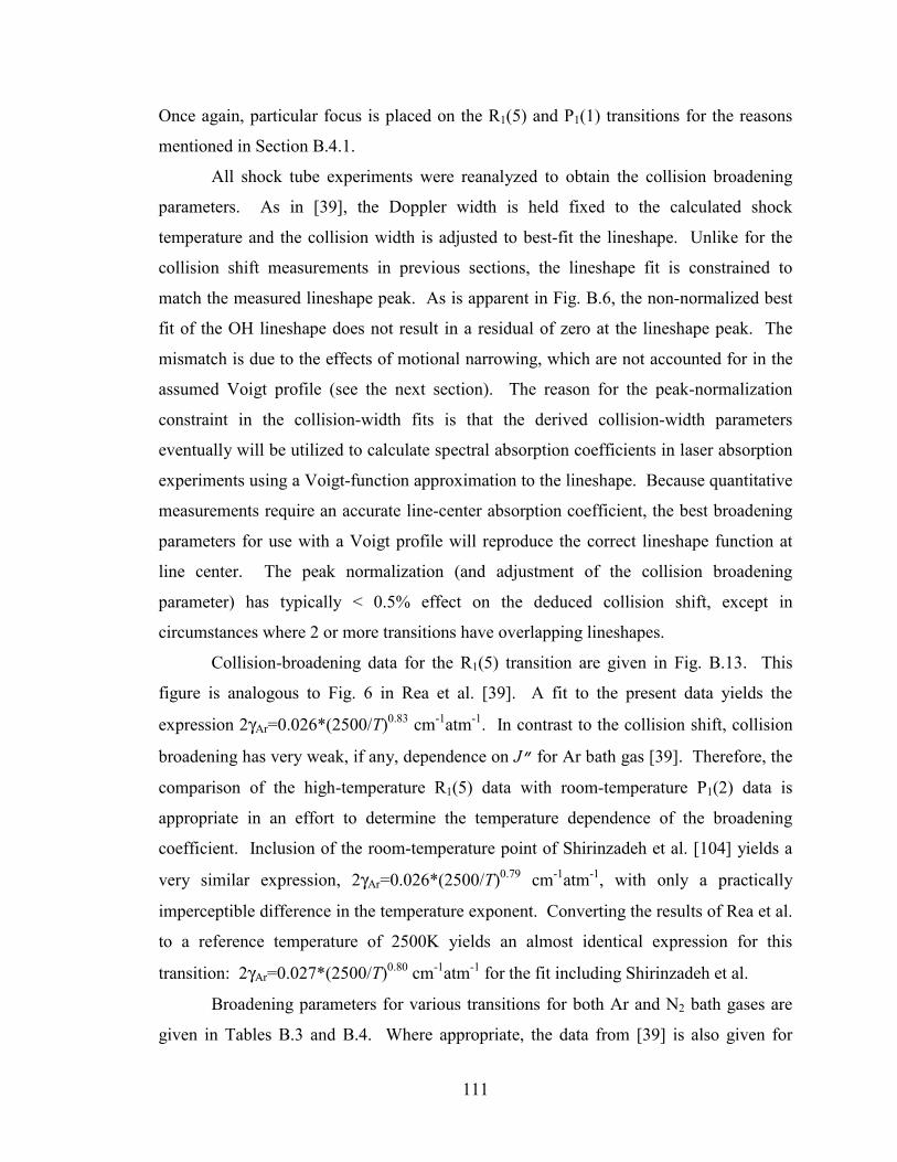
111

Once again, particular focus is placed on the R1(5) and P1(1) transitions for the reasons

mentioned in Section B.4.1.

All shock tube experiments were reanalyzed to obtain the collision broadening

parameters. As in [39], the Doppler width is held fixed to the calculated shock

temperature and the collision width is adjusted to best-fit the lineshape. Unlike for the

collision shift measurements in previous sections, the lineshape fit is constrained to

match the measured lineshape peak. As is apparent in Fig. B.6, the non-normalized best

fit of the OH lineshape does not result in a residual of zero at the lineshape peak. The

mismatch is due to the effects of motional narrowing, which are not accounted for in the

assumed Voigt profile (see the next section). The reason for the peak-normalization

constraint in the collision-width fits is that the derived collision-width parameters

eventually will be utilized to calculate spectral absorption coefficients in laser absorption

experiments using a Voigt-function approximation to the lineshape. Because quantitative

measurements require an accurate line-center absorption coefficient, the best broadening

parameters for use with a Voigt profile will reproduce the correct lineshape function at

line center. The peak normalization (and adjustment of the collision broadening

parameter) has typically < 0.5% effect on the deduced collision shift, except in

circumstances where 2 or more transitions have overlapping lineshapes.

Collision-broadening data for the R1(5) transition are given in Fig. B.13. This

figure is analogous to Fig. 6 in Rea et al. [39]. A fit to the present data yields the

expression 2γAr=0.026*(2500/T)0.83 cm-1atm-1. In contrast to the collision shift, collision

broadening has very weak, if any, dependence on J” for Ar bath gas [39]. Therefore, the

comparison of the high-temperature R1(5) data with room-temperature P1(2) data is

appropriate in an effort to determine the temperature dependence of the broadening

coefficient. Inclusion of the room-temperature point of Shirinzadeh et al. [104] yields a

very similar expression, 2γAr=0.026*(2500/T)0.79 cm-1atm-1, with only a practically

imperceptible difference in the temperature exponent. Converting the results of Rea et al.

to a reference temperature of 2500K yields an almost identical expression for this

transition: 2γAr=0.027*(2500/T)0.80 cm-1atm-1 for the fit including Shirinzadeh et al.

Broadening parameters for various transitions for both Ar and N2 bath gases are

given in Tables B.3 and B.4. Where appropriate, the data from [39] is also given for

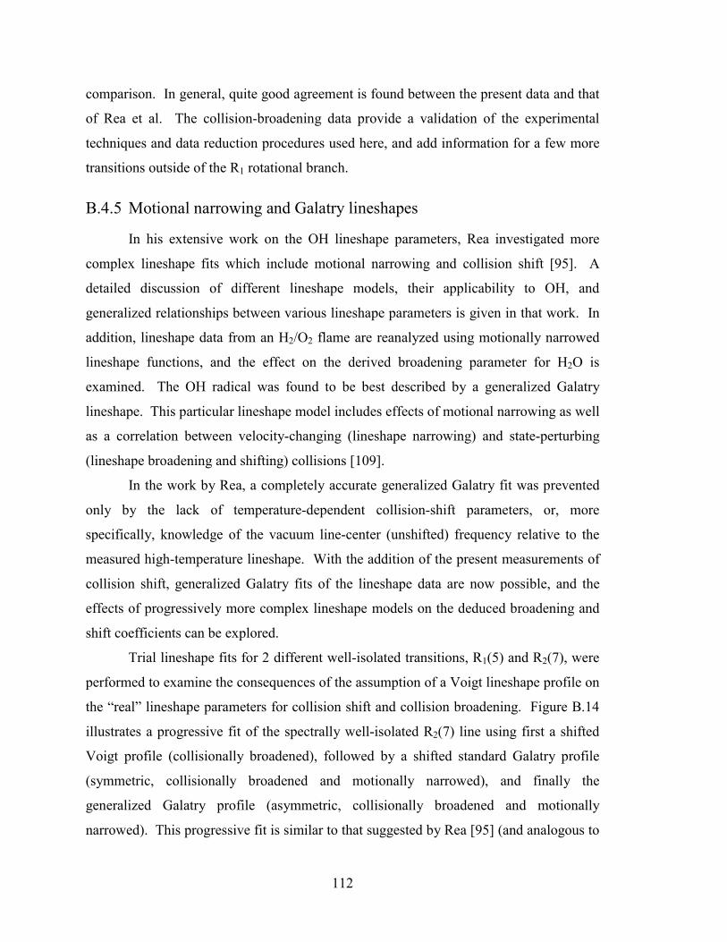
112

comparison. In general, quite good agreement is found between the present data and that

of Rea et al. The collision-broadening data provide a validation of the experimental

techniques and data reduction procedures used here, and add information for a few more

transitions outside of the R1 rotational branch.

B.4.5 Motional narrowing and Galatry lineshapes

In his extensive work on the OH lineshape parameters, Rea investigated more

complex lineshape fits which include motional narrowing and collision shift [95]. A

detailed discussion of different lineshape models, their applicability to OH, and

generalized relationships between various lineshape parameters is given in that work. In

addition, lineshape data from an H2/O2 flame are reanalyzed using motionally narrowed

lineshape functions, and the effect on the derived broadening parameter for H2O is

examined. The OH radical was found to be best described by a generalized Galatry

lineshape. This particular lineshape model includes effects of motional narrowing as well

as a correlation between velocity-changing (lineshape narrowing) and state-perturbing

(lineshape broadening and shifting) collisions [109].

In the work by Rea, a completely accurate generalized Galatry fit was prevented

only by the lack of temperature-dependent collision-shift parameters, or, more

specifically, knowledge of the vacuum line-center (unshifted) frequency relative to the

measured high-temperature lineshape. With the addition of the present measurements of

collision shift, generalized Galatry fits of the lineshape data are now possible, and the

effects of progressively more complex lineshape models on the deduced broadening and

shift coefficients can be explored.

Trial lineshape fits for 2 different well-isolated transitions, R1(5) and R2(7), were

performed to examine the consequences of the assumption of a Voigt lineshape profile on

the “real” lineshape parameters for collision shift and collision broadening. Figure B.14

illustrates a progressive fit of the spectrally well-isolated R2(7) line using first a shifted

Voigt profile (collisionally broadened), followed by a shifted standard Galatry profile

(symmetric, collisionally broadened and motionally narrowed), and finally the

generalized Galatry profile (asymmetric, collisionally broadened and motionally

narrowed). This progressive fit is similar to that suggested by Rea [95] (and analogous to

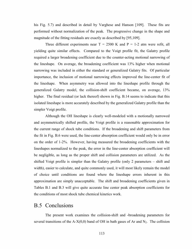
113

his Fig. 5.7) and described in detail by Varghese and Hanson [109]. These fits are

performed without normalization of the peak. The progressive change in the shape and

magnitude of the fitting residuals are exactly as described by [95,109].

Three different experiments near T = 2500 K and P = 1-2 atm were refit, all

yielding quite similar effects. Compared to the Voigt profile fit, the Galatry profile

required a larger broadening coefficient due to the counter-acting motional narrowing of

the lineshape. On average, the broadening coefficient was 13% higher when motional

narrowing was included in either the standard or generalized Galatry fits. Of particular

importance, the inclusion of motional narrowing effects improved the line-center fit of

the lineshape. When asymmetry was allowed into the lineshape profile through the

generalized Galatry model, the collision-shift coefficient became, on average, 13%

higher. The final residual (or lack thereof) shown in Fig. B.14 seems to indicate that this

isolated lineshape is more accurately described by the generalized Galatry profile than the

simpler Voigt profile.

Although the OH lineshape is clearly well-modeled with a motionally narrowed

and asymmetrically shifted profile, the Voigt profile is a reasonable approximation for

the current range of shock tube conditions. If the broadening and shift parameters from

the fit in Fig. B.6 were used, the line-center absorption coefficient would only be in error

on the order of 1-2%. However, having measured the broadening coefficients with the

lineshapes normalized to the peak, the error in the line-center absorption coefficient will

be negligible, as long as the proper shift and collision parameters are utilized. As the

shifted Voigt profile is simpler than the Galatry profile (only 2 parameters – shift and

width), easier to calculate, and quite commonly used, it will most likely remain the model

of choice until conditions are found where the lineshape errors inherent in this

approximation are simply unacceptable. The shift and broadening coefficients given in

Tables B.1 and B.3 will give quite accurate line center peak absorption coefficients for

the conditions of most shock tube chemical kinetics work.

B.5 Conclusions The present work examines the collision-shift and -broadening parameters for

several transitions of the A-X(0,0) band of OH in bath gases of Ar and N2. The collision

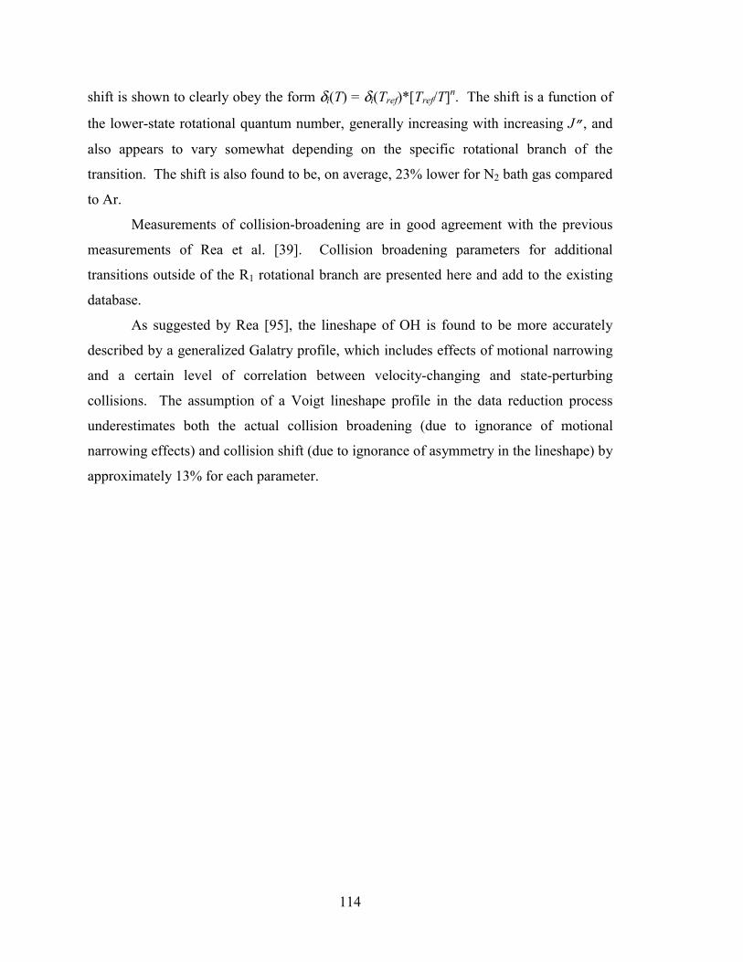
114

shift is shown to clearly obey the form δi(T) = δi(Tref)*[Tref/T]n. The shift is a function of

the lower-state rotational quantum number, generally increasing with increasing J”, and

also appears to vary somewhat depending on the specific rotational branch of the

transition. The shift is also found to be, on average, 23% lower for N2 bath gas compared

to Ar.

Measurements of collision-broadening are in good agreement with the previous

measurements of Rea et al. [39]. Collision broadening parameters for additional

transitions outside of the R1 rotational branch are presented here and add to the existing

database.

As suggested by Rea [95], the lineshape of OH is found to be more accurately

described by a generalized Galatry profile, which includes effects of motional narrowing

and a certain level of correlation between velocity-changing and state-perturbing

collisions. The assumption of a Voigt lineshape profile in the data reduction process

underestimates both the actual collision broadening (due to ignorance of motional

narrowing effects) and collision shift (due to ignorance of asymmetry in the lineshape) by

approximately 13% for each parameter.

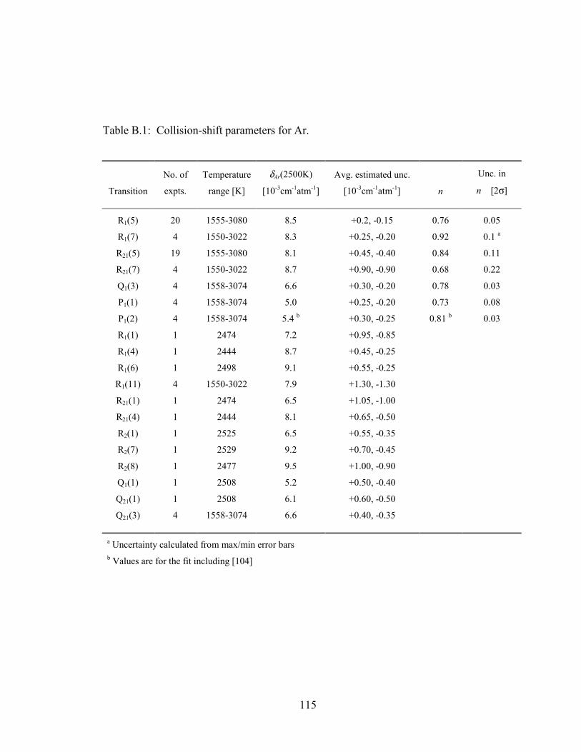
115

Table B.1: Collision-shift parameters for Ar.

Transition

No. of

expts.

Temperature

range [K]

δAr(2500K)

[10-3cm-1atm-1]

Avg. estimated unc.

[10-3cm-1atm-1] n

Unc. in

n [2σ]

R1(5) 20 1555-3080 8.5 +0.2, -0.15 0.76 0.05

R1(7) 4 1550-3022 8.3 +0.25, -0.20 0.92 0.1 a

R21(5) 19 1555-3080 8.1 +0.45, -0.40 0.84 0.11

R21(7) 4 1550-3022 8.7 +0.90, -0.90 0.68 0.22

Q1(3) 4 1558-3074 6.6 +0.30, -0.20 0.78 0.03

P1(1) 4 1558-3074 5.0 +0.25, -0.20 0.73 0.08

P1(2) 4 1558-3074 5.4 b +0.30, -0.25 0.81 b 0.03

R1(1) 1 2474 7.2 +0.95, -0.85

R1(4) 1 2444 8.7 +0.45, -0.25

R1(6) 1 2498 9.1 +0.55, -0.25

R1(11) 4 1550-3022 7.9 +1.30, -1.30

R21(1) 1 2474 6.5 +1.05, -1.00

R21(4) 1 2444 8.1 +0.65, -0.50

R2(1) 1 2525 6.5 +0.55, -0.35

R2(7) 1 2529 9.2 +0.70, -0.45

R2(8) 1 2477 9.5 +1.00, -0.90

Q1(1) 1 2508 5.2 +0.50, -0.40

Q21(1) 1 2508 6.1 +0.60, -0.50

Q21(3) 4 1558-3074 6.6 +0.40, -0.35

a Uncertainty calculated from max/min error bars b Values are for the fit including [104]

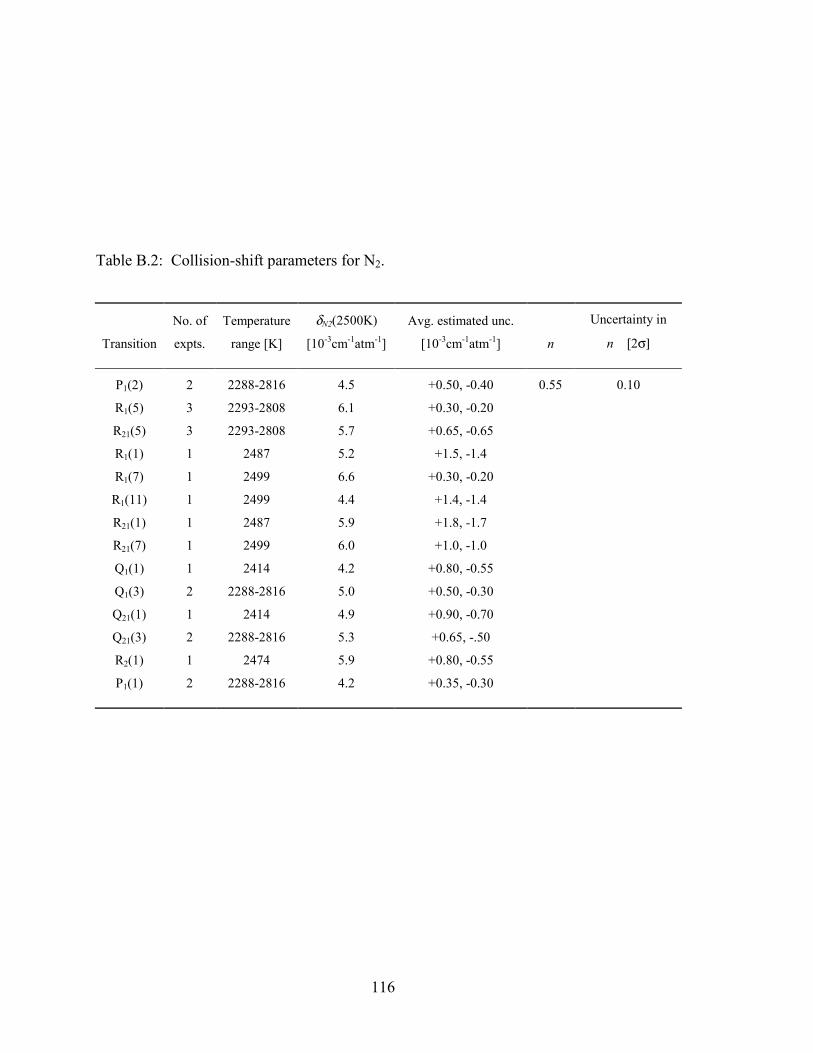
116

Table B.2: Collision-shift parameters for N2.

Transition

No. of

expts.

Temperature

range [K]

δN2(2500K)

[10-3cm-1atm-1]

Avg. estimated unc.

[10-3cm-1atm-1] n

Uncertainty in

n [2σ]

P1(2) 2 2288-2816 4.5 +0.50, -0.40 0.55 0.10

R1(5) 3 2293-2808 6.1 +0.30, -0.20

R21(5) 3 2293-2808 5.7 +0.65, -0.65

R1(1) 1 2487 5.2 +1.5, -1.4

R1(7) 1 2499 6.6 +0.30, -0.20

R1(11) 1 2499 4.4 +1.4, -1.4

R21(1) 1 2487 5.9 +1.8, -1.7

R21(7) 1 2499 6.0 +1.0, -1.0

Q1(1) 1 2414 4.2 +0.80, -0.55

Q1(3) 2 2288-2816 5.0 +0.50, -0.30

Q21(1) 1 2414 4.9 +0.90, -0.70

Q21(3) 2 2288-2816 5.3 +0.65, -.50

R2(1) 1 2474 5.9 +0.80, -0.55

P1(1) 2 2288-2816 4.2 +0.35, -0.30

117

Table B.3: Collision-broadening parameters for Ar.

This study only Rea et al. [39]

Transition

No. of

expts.

Temperature

range [K]

2γAr(2500K)

[cm-1atm-1] n

With

[104]

n 2γAr(2500K) n

With

[104]

n

R1(5) 20 1555-3080 0.026 0.83 0.79 0.027 0.92 0.8

R1(7) 4 1550-3022 0.023 1.01 0.86 0.028 1.13 0.8

R1(11) 4 1550-3022 0.030 0.83 0.73 0.028 1.1 0.8

P1(1) 4 1558-3074 0.027 0.90 0.78

R21(5) 19 1555-3080 0.027 0.88 0.78

Q1(3) 4 1558-3074 0.026 0.78 0.79

Q21(3) 4 1558-3074 0.025 0.90 0.80

Table B.4: Collision-broadening parameters for N2.

This study only Rea et al. [39] only

Transition

No. of

expts.

Temperature

range [K]

2γN2(2500K)

[cm-1atm-1] n

With [104]

n 2γN2(2500K) n

With

[104]

n

R1(5) 4 2051-2808 0.033 0.58 0.88 0.038 0.54 0.83

R1(7) 1 2499 0.029 0.034 0.72 0.89

R1(11) 1 2499 0.029 0.029 0.74 0.97

R21(5) 4 2051-2808 0.033 0.71 0.88

P1(1) 2 2288-2816 0.035 0.86

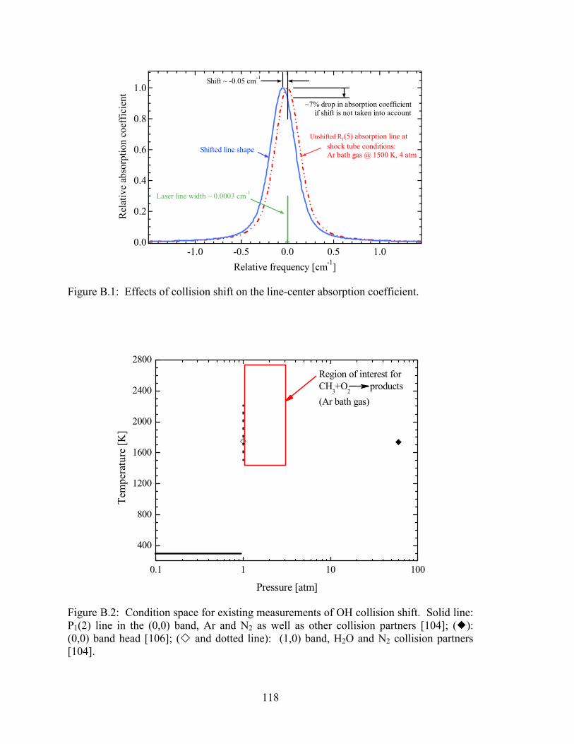
118

1.0

0.8

0.6

0.4

0.2

0.0

Rel

ativ

e ab

sorp

tion

coef

ficie

nt

-1.0 -0.5 0.0 0.5 1.0Relative frequency [cm-1]

Shift ~ -0.05 cm-1

~7% drop in absorption coefficient if shift is not taken into account

Unshifted R1(5) absorption line at shock tube conditions: Ar bath gas @ 1500 K, 4 atm

Shifted line shape

Laser line width ~ 0.0003 cm-1

Figure B.1: Effects of collision shift on the line-center absorption coefficient.

0.1 1 10 100

400

800

1200

1600

2000

2400

2800Region of interest for CH

3+O

2 products

(Ar bath gas)

Tem

pera

ture

[K]

Pressure [atm]

Figure B.2: Condition space for existing measurements of OH collision shift. Solid line: P1(2) line in the (0,0) band, Ar and N2 as well as other collision partners [104]; (�): (0,0) band head [106]; (� and dotted line): (1,0) band, H2O and N2 collision partners [104].

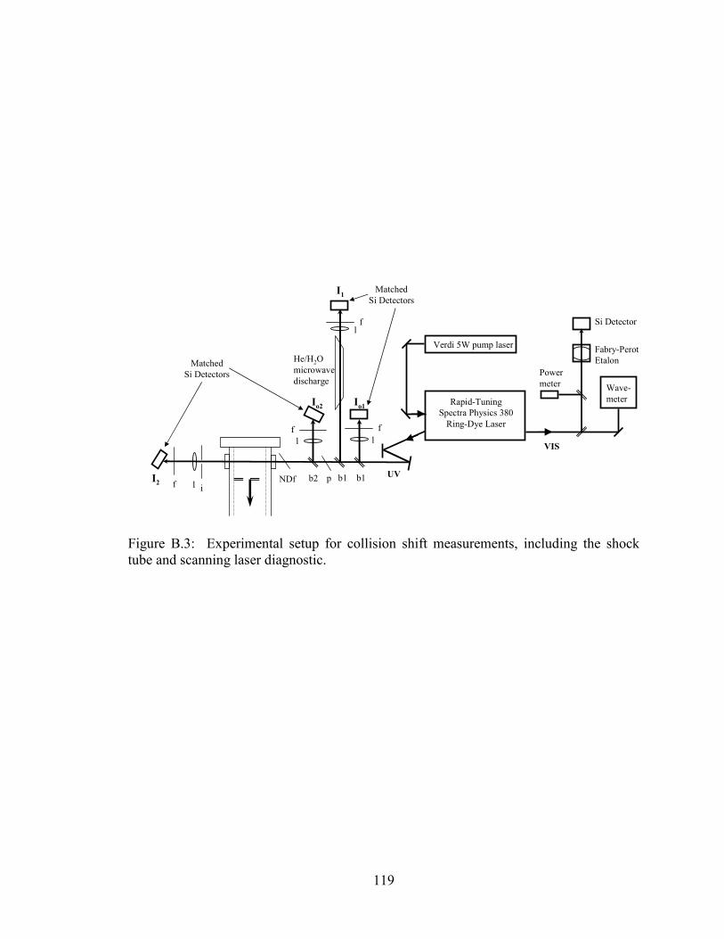
119

Verdi 5W pump laser

Rapid-TuningSpectra Physics 380

Ring-Dye Laser

Powermeter

Fabry-PerotEtalon

Si Detector

VIS

UV

Wave-meter

MatchedSi Detectors

He/H2O microwavedischarge

f l

f

f

lf

MatchedSi Detectors

Io1

I1

Io2

I2 NDf

l

l

pi

b1 b1b2

Figure B.3: Experimental setup for collision shift measurements, including the shock tube and scanning laser diagnostic.

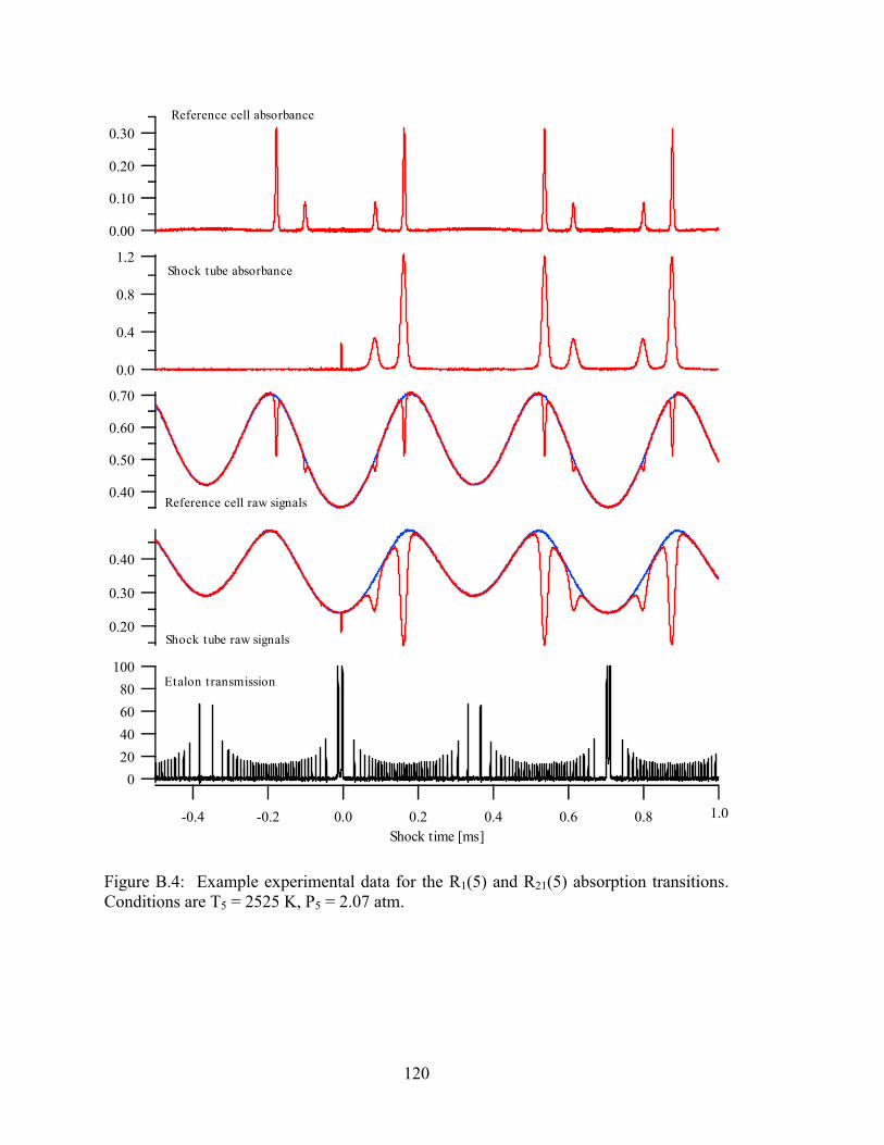
120

100806040200

1.0x100.80.60.40.20.0-0.2-0.4Shock time [ms]

0.40

0.30

0.20

0.70

0.60

0.50

0.40

1.2

0.8

0.4

0.0

0.30

0.20

0.10

0.00

Shock tube raw signals

Reference cell raw signals

Shock tube absorbance

Reference cell absorbance

1.0

Etalon t ransmission

Figure B.4: Example experimental data for the R1(5) and R21(5) absorption transitions. Conditions are T5 = 2525 K, P5 = 2.07 atm.

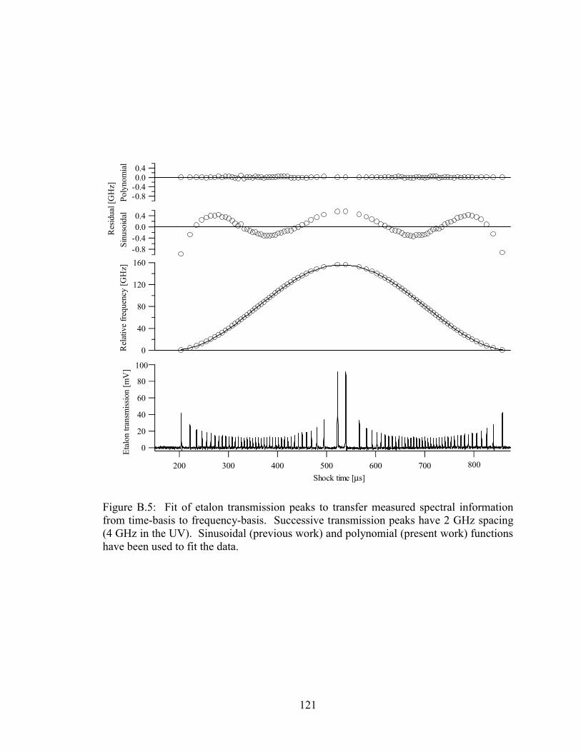
121

160

120

80

40

0Rel

ativ

e fre

quen

cy [G

Hz]

800x10-6 700600500400300200Shock time [µs]

100x10-3

80

60

40

20

0Etal

on tr

ansm

issio

n [m

V]

-0.8-0.40.00.4

Res

idua

l [G

Hz]

-0.8-0.40.00.4

800

100

Sinu

soid

al

Pol

ynom

ial

Figure B.5: Fit of etalon transmission peaks to transfer measured spectral information from time-basis to frequency-basis. Successive transmission peaks have 2 GHz spacing (4 GHz in the UV). Sinusoidal (previous work) and polynomial (present work) functions have been used to fit the data.

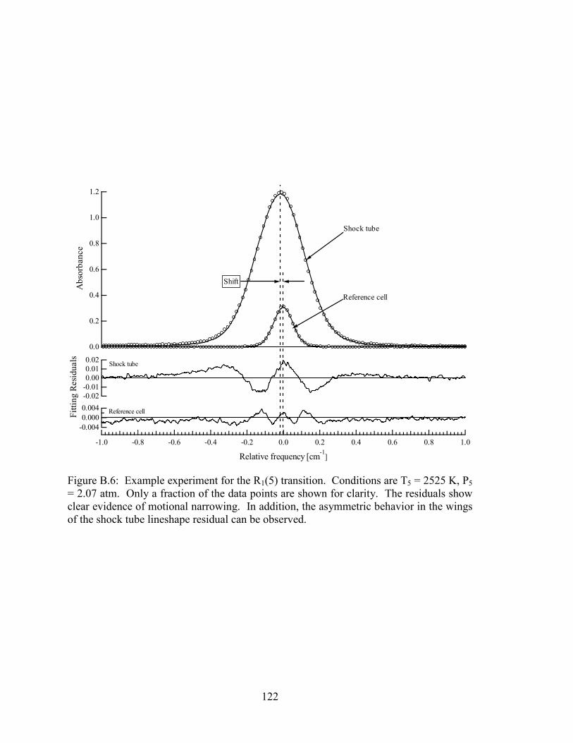
122

1.2

1.0

0.8

0.6

0.4

0.2

0.0

Abs

orba

nce

-1.0 -0.8 -0.6 -0.4 -0.2 0.0 0.2 0.4 0.6 0.8 1.0

Relative frequency [cm-1]

-0.0040.0000.004-0.02-0.010.000.010.02

Fitti

ng R

esid

uals Shock tube

Reference cell

Shock tube

Reference cell

Shift

Figure B.6: Example experiment for the R1(5) transition. Conditions are T5 = 2525 K, P5 = 2.07 atm. Only a fraction of the data points are shown for clarity. The residuals show clear evidence of motional narrowing. In addition, the asymmetric behavior in the wings of the shock tube lineshape residual can be observed.

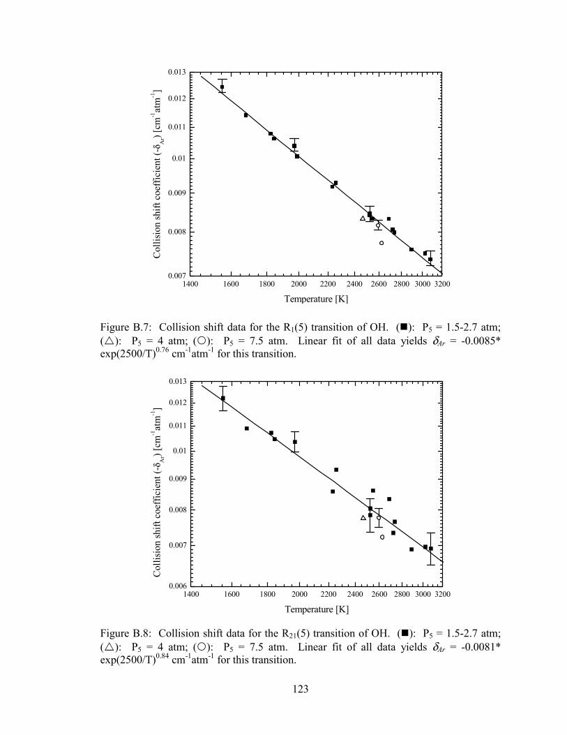
123

1400 1600 1800 2000 2200 2400 2600 2800 3000 32000.007

0.008

0.009

0.01

0.011

0.012

0.013

Col

lisio

n sh

ift c

oeff

icie

nt (-

δ Ar) [

cm-1at

m-1]

Temperature [K]

Figure B.7: Collision shift data for the R1(5) transition of OH. (�): P5 = 1.5-2.7 atm; (�): P5 = 4 atm; (�): P5 = 7.5 atm. Linear fit of all data yields δAr = -0.0085* exp(2500/T)0.76 cm-1atm-1 for this transition.

1400 1600 1800 2000 2200 2400 2600 2800 3000 32000.006

0.007

0.008

0.009

0.01

0.011

0.012

0.013

Col

lisio

n sh

ift c

oeff

icie

nt (-

δ Ar) [

cm-1at

m-1]

Temperature [K]

Figure B.8: Collision shift data for the R21(5) transition of OH. (�): P5 = 1.5-2.7 atm; (�): P5 = 4 atm; (�): P5 = 7.5 atm. Linear fit of all data yields δAr = -0.0081* exp(2500/T)0.84 cm-1atm-1 for this transition.

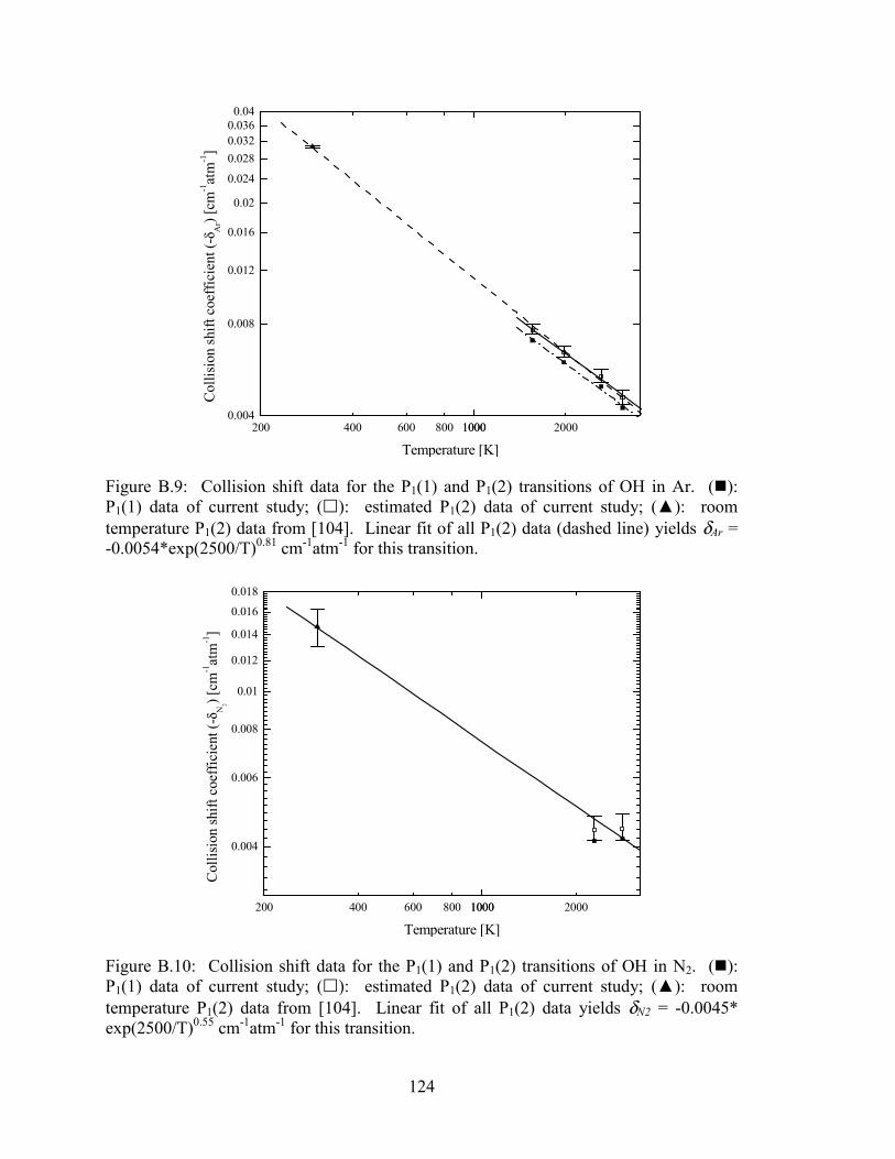
124

200 400 600 800 10001000 20000.004

0.008

0.012

0.016

0.02

0.024

0.0280.0320.0360.04

Col

lisio

n sh

ift c

oeff

icie

nt (-

δ Ar) [

cm-1at

m-1]

Temperature [K]

Figure B.9: Collision shift data for the P1(1) and P1(2) transitions of OH in Ar. (�): P1(1) data of current study; (�): estimated P1(2) data of current study; (▲): room temperature P1(2) data from [104]. Linear fit of all P1(2) data (dashed line) yields δAr = -0.0054*exp(2500/T)0.81 cm-1atm-1 for this transition.

200 400 600 800 10001000 2000

0.004

0.006

0.008

0.01

0.012

0.014

0.016

0.018

Col

lisio

n sh

ift c

oeff

icie

nt (-

δ N2) [

cm-1at

m-1]

Temperature [K]

Figure B.10: Collision shift data for the P1(1) and P1(2) transitions of OH in N2. (�): P1(1) data of current study; (�): estimated P1(2) data of current study; (▲): room temperature P1(2) data from [104]. Linear fit of all P1(2) data yields δN2 = -0.0045* exp(2500/T)0.55 cm-1atm-1 for this transition.

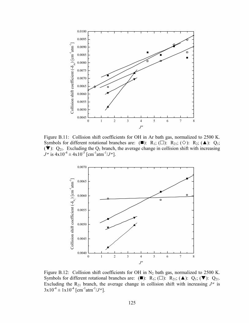
125

0 1 2 3 4 5 6 7 80.0045

0.0050

0.0055

0.0060

0.0065

0.0070

0.0075

0.0080

0.0085

0.0090

0.0095

0.0100

Col

lisio

n sh

ift c

oeff

icie

nt (-

δ Ar) [

cm-1at

m-1]

J"

Figure B.11: Collision shift coefficients for OH in Ar bath gas, normalized to 2500 K. Symbols for different rotational branches are: (�): R1; (�): R21; (�): R2; (▲): Q1; (�): Q21. Excluding the Q1 branch, the average change in collision shift with increasing J” is 4x10-4 ± 4x10-5 [cm-1atm-1/J”].

0 1 2 3 4 5 6 7 80.0040

0.0045

0.0050

0.0055

0.0060

0.0065

0.0070

Col

lisio

n sh

ift c

oeff

icie

nt (-

δ N2) [

cm-1at

m-1]

J"

Figure B.12: Collision shift coefficients for OH in N2 bath gas, normalized to 2500 K. Symbols for different rotational branches are: (�): R1; (�): R21; (▲): Q1; (�): Q21. Excluding the R21 branch, the average change in collision shift with increasing J” is 3x10-4 ± 1x10-4 [cm-1atm-1/J”].

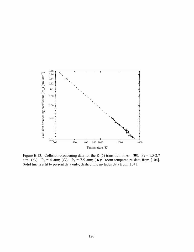
126

200 400 600 800 1000 2000 40000.02

0.04

0.06

0.08

0.1

0.12

0.140.160.18

Col

lisio

n br

oade

ning

coe

ffici

ent (

2γA

r) [cm

-1at

m-1]

Temperature [K]

Figure B.13: Collision-broadening data for the R1(5) transition in Ar. (�): P5 = 1.5-2.7 atm; (�): P5 = 4 atm; (�): P5 = 7.5 atm; (▲): room-temperature data from [104]. Solid line is a fit to present data only; dashed line includes data from [104].

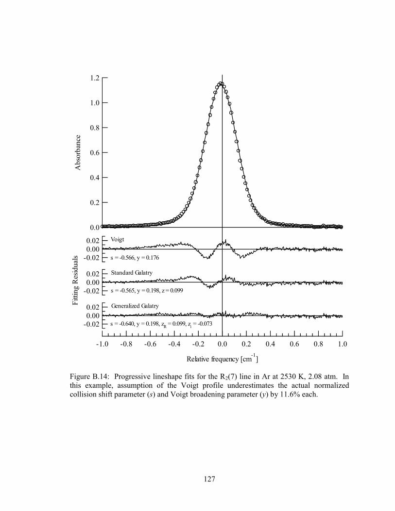
127

1.2

1.0

0.8

0.6

0.4

0.2

0.0

Abs

orba

nce

-1.0 -0.8 -0.6 -0.4 -0.2 0.0 0.2 0.4 0.6 0.8 1.0

Relative frequency [cm-1]

-0.020.000.02

-0.020.000.02

Fitti

ng R

esid

uals

-0.020.000.02

Voigt

Standard Galatry

Generalized Galatry

s = -0.566, y = 0.176

s = -0.565, y = 0.198, z = 0.099

s = -0.640, y = 0.198, zR = 0.099, zi = -0.073

Figure B.14: Progressive lineshape fits for the R2(7) line in Ar at 2530 K, 2.08 atm. In this example, assumption of the Voigt profile underestimates the actual normalized collision shift parameter (s) and Voigt broadening parameter (y) by 11.6% each.

129

Appendix C: Shock velocity and T5, P5 uncertainty analysis

This appendix describes an analysis for estimating the uncertainty in the

calculated ideal shock conditions immediately behind the reflected shock wave, based on

estimated uncertainties in various measured parameters as well as the quality of the shock

velocity measurement.

C.1 Motivation The accurate knowledge of post-shock temperatures and pressures in shock tube

chemical kinetics experiments is critical to successful measurements of rate coefficient

parameters. This issue was clearly demonstrated in Section 3.5.1, where a difference of

25 K (~1.5 %) was found to be the primary cause of a factor of three discrepancy in the

reported results for k1a from two previous investigations.

The determination of the correct temperature and pressure is typically separated

into two parts. The first concern is the calculation of the ideal shock conditions

immediately behind the shock wave at the test location (optical diagnostic ports), based

on an accurate determination of the incident shock wave velocity and the initial

conditions. Any non-ideal effects must subsequently be taken into account, including

temperature and pressure changes with time due to chemical heat release, boundary layer

growth behind the incident shock wave, and vibrational relaxation of the shocked gases.

For the work in this thesis, chemical heat release was not an issue due to the very low

concentration mixtures utilized. However, in other experimental situations the heat

release is typically accounted for during the chemical modeling of the experiment by

assuming that constant U,V conditions apply. Boundary layer effects were assumed to be

negligible in the post-shock regime (due to the large shock tube diameter – see Section

3.5.1). The attenuation of the incident shock wave is accounted for in the shock velocity

130

linear regression analysis (see below). Finally, vibrational relaxation effects, typically

affecting mixtures with large concentrations of diatomic species, can be minimized by

decreasing the mole fraction of diatomics and adding helium or other light gases to speed

up the relaxation process. When these options are not suitable, published relaxation-time

relationships for various relaxing-gas/bath-gas combinations can be used to estimate the

relaxation rate from vibrationally frozen to vibrationally equilibrated temperature and

pressure conditions [51].

This appendix will focus only on the calculation of the ideal shock conditions

immediately behind the reflected shock wave and the estimated uncertainties in that

calculation.

C.2 Shock velocity measurement and uncertainty

calculation The conditions immediately behind the reflected shock wave are calculated using

the well-known ideal shock relations [110]:

( ) ( )( )

( ) ( )[ ]12131

312 222

2

15 −−−

+−+−= γγ

γγγ M

MMTT (C.1)

( ) ( ) ( )( )

+−−−−

+−−=

211213

112

2

22

15 MMMPP

γγγ

γγγ (C.2)

where M = incident shock Mach number ≡ V/a1, and a1 = the speed of sound at the initial

conditions ≡ (γRT1)1/2. Input parameters in these equations which must be measured for

each experiment include the shock velocity at the endwall, Vendwall, the initial temperature,

T1, and the initial pressure, P1. The ratio of specific heats, γ, is determined from the

thermodynamic data of the mixture species.

The initial conditions T1 and P1 are measured before each experiment, and the

instrument uncertainties can be estimated for each of these quantities. The specific heat

ratio, γ, is assumed to have negligible uncertainty. The shock velocity is the most critical

parameter, and an analysis is developed here to understand the uncertainty in its

measurement.

131

The shock velocity is measured using five PCB Piezotronics piezoelectric

pressure transducers (PZT’s) connected to four interval timers with 0.1 µs time-

resolution. The pressure rise in the incident shock wave at successive PZT’s triggers the

start and end for each interval timer. The four velocity measurements are fit to a linear

regression and extrapolated to the endwall to determine the velocity at the endwall. The

gas volume at the optical test ports, located only 2 cm from the endwall, is assumed to

obtain conditions very similar those at the endwall. Uncertain quantities in the

determination of Vendwall are therefore the interval distances, dxi, the interval times, dti,

and the location of the endwall, xendwall. The dxi uncertainty was estimated at δx ≈ ±0.25

mm, based on a ±0.12 mm tolerance in the location dimensions for each PZT port. The

dti uncertainty was assessed by performing experiments in which all five transducers

were mounted at the same plane along the shock tube axis. The variation in the time at

which each PZT reached the trigger-threshold voltage gives an indication of the potential

error due to individual PZT time response. Results of one of these experiments are

shown in Fig. C.1. Based on a few shocks at various conditions, the spread between the

earliest and latest PZT time response at the trigger threshold appeared to be near δt ≈ 0.7

µs . While a specific PZT may tend to be consistently later or earlier than others, in

general it was observed that relative positions of the PZT’s did not necessarily remain

constant from shock to shock. Therefore, the maximum spread was retained as the

estimated uncertainty in the measured time intervals due to the potential time response

difference of two consecutive PZT’s.

A spreadsheet was developed to perform a weighted linear regression analysis of

the incident shock velocity measurements and to analyze the uncertainty in the

determination of the endwall shock velocity. The equations used here follow the linear

regression analysis discussion in Bevington and Robinson [111]. The incident shock

wave velocity at each measurement point i (mid-way between successive PZT’s) is

determined quite simply by:

i

iii dt

dxyV == (C.3)

Estimated uncertainties for each velocity point, σi, can be calculated based on assumed

uncertainties in dti and dxi :

132

21

22

+

=

iiii dt

tdx

xV δδσ (C.4)

Using the estimated uncertainties as weighting factors and assuming initial guesses for

the linear fit parameters a and b, a goodness-of-fit parameter, χ2, can be calculated:

( )( )∑

−−=

iii

i

bxay2

2 1σ

χ (C.5)

The optimum fit is determined by the parameters a and b that minimize the weighted sum

of the squares of the deviations, χ2 (i.e., a “least-squares” fit). The parameters a and b

can be found by setting to zero the partial derivatives of χ2 with respect to each of the

parameters. Rearranging them into a pair of linear simultaneous equations in a and b, the

solution can be found using the method of determinants. The problem is reduced to

directly solving the following equations:

−

∆= ∑ ∑ ∑∑ 2222

21

i

ii

i

i

i

i

i

i yxxyxa

σσσσ (C.6)

−

∆= ∑ ∑ ∑ ∑ 2222

11

i

i

i

i

i

ii

i

yxyxb

σσσσ (C.7)

∑ ∑ ∑

−=∆

2

22

2

2

1

i

i

i

i

i

xxσσσ

(C.8)

The standard deviation for the fit, σ, can be calculated based on the scatter in the linear

regression:

( )∑ −−−

= 22

21

ii bxayN

σ (C.9)

where N is the number of data points. If the uncertainties used to calculate σi have been

appropriately estimated, and if σi is approximately the same for all points, σ should be

approximately equal to σi. Substituting σ from Equation (C.9) into Equation (C.5) yields

χ2 ≈ (N – 2). So, if in Equation (C.5) χ2 < (N – 2), the uncertainty in one or more

parameters has been overestimated; conversely if χ2 > (N – 2), the scatter in the velocity

data indicates the presence of higher random uncertainties than the estimated uncertainty

suggests. The error in the time interval measurement dti is the dominant uncertainty.

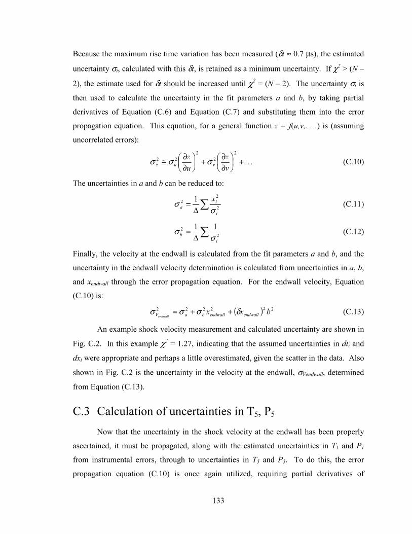
133

Because the maximum rise time variation has been measured (δt ≈ 0.7 µs), the estimated

uncertainty σi, calculated with this δt, is retained as a minimum uncertainty. If χ2 > (N –

2), the estimate used for δt should be increased until χ2 = (N – 2). The uncertainty σi is

then used to calculate the uncertainty in the fit parameters a and b, by taking partial

derivatives of Equation (C.6) and Equation (C.7) and substituting them into the error

propagation equation. This equation, for a general function z = f(u,v,. . .) is (assuming

uncorrelated errors):

l+

∂∂+

∂∂≅

22

222

vz

uz

vuz σσσ (C.10)

The uncertainties in a and b can be reduced to:

∑∆= 2

22 1

i

ia

xσ

σ (C.11)

∑∆= 2

2 11

ib σ

σ (C.12)

Finally, the velocity at the endwall is calculated from the fit parameters a and b, and the

uncertainty in the endwall velocity determination is calculated from uncertainties in a, b,

and xendwall through the error propagation equation. For the endwall velocity, Equation

(C.10) is:

( ) 222222 bxx endwallendwallbaVendwallδσσσ ++= (C.13)

An example shock velocity measurement and calculated uncertainty are shown in

Fig. C.2. In this example χ2 = 1.27, indicating that the assumed uncertainties in dti and

dxi were appropriate and perhaps a little overestimated, given the scatter in the data. Also

shown in Fig. C.2 is the uncertainty in the velocity at the endwall, σVendwall, determined

from Equation (C.13).

C.3 Calculation of uncertainties in T5, P5 Now that the uncertainty in the shock velocity at the endwall has been properly

ascertained, it must be propagated, along with the estimated uncertainties in T1 and P1

from instrumental errors, through to uncertainties in T5 and P5. To do this, the error

propagation equation (C.10) is once again utilized, requiring partial derivatives of

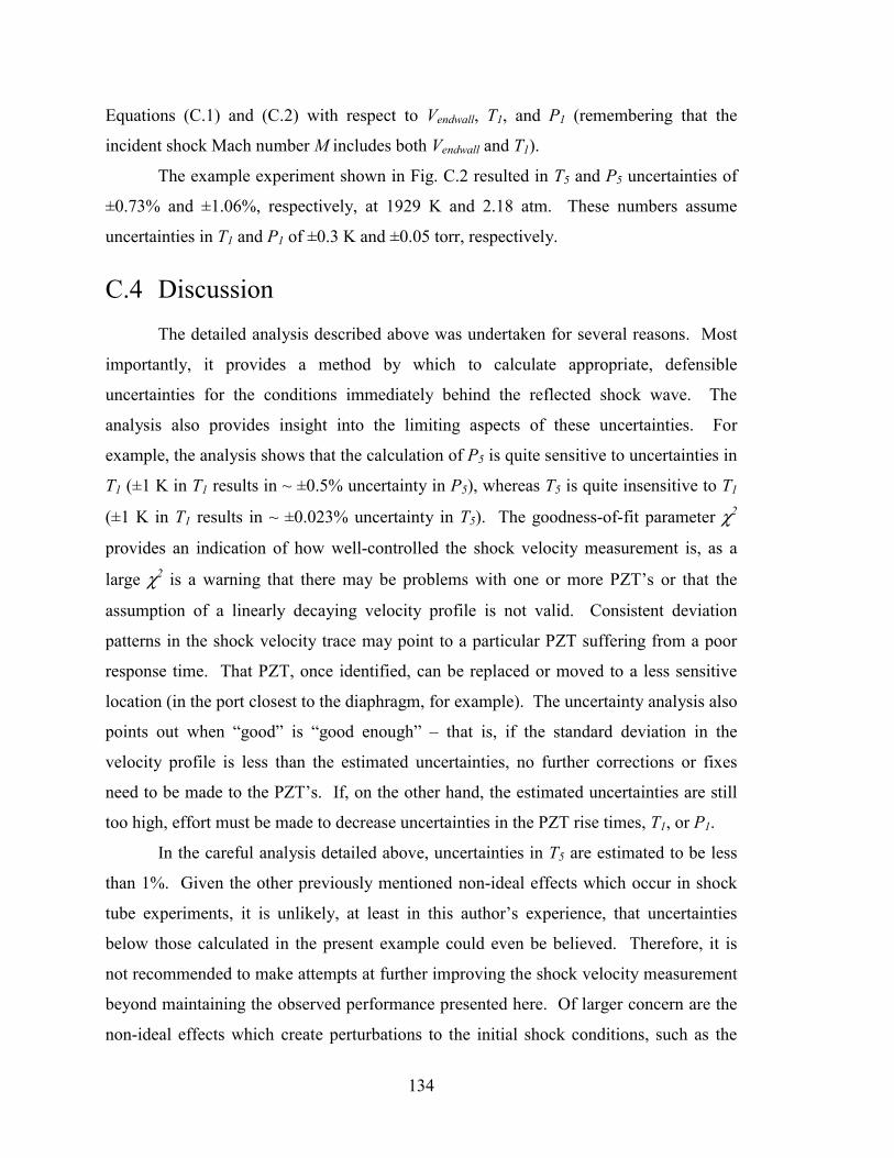
134

Equations (C.1) and (C.2) with respect to Vendwall, T1, and P1 (remembering that the

incident shock Mach number M includes both Vendwall and T1).

The example experiment shown in Fig. C.2 resulted in T5 and P5 uncertainties of

±0.73% and ±1.06%, respectively, at 1929 K and 2.18 atm. These numbers assume

uncertainties in T1 and P1 of ±0.3 K and ±0.05 torr, respectively.

C.4 Discussion The detailed analysis described above was undertaken for several reasons. Most

importantly, it provides a method by which to calculate appropriate, defensible

uncertainties for the conditions immediately behind the reflected shock wave. The

analysis also provides insight into the limiting aspects of these uncertainties. For

example, the analysis shows that the calculation of P5 is quite sensitive to uncertainties in

T1 (±1 K in T1 results in ~ ±0.5% uncertainty in P5), whereas T5 is quite insensitive to T1

(±1 K in T1 results in ~ ±0.023% uncertainty in T5). The goodness-of-fit parameter χ2

provides an indication of how well-controlled the shock velocity measurement is, as a

large χ2 is a warning that there may be problems with one or more PZT’s or that the

assumption of a linearly decaying velocity profile is not valid. Consistent deviation

patterns in the shock velocity trace may point to a particular PZT suffering from a poor

response time. That PZT, once identified, can be replaced or moved to a less sensitive

location (in the port closest to the diaphragm, for example). The uncertainty analysis also

points out when “good” is “good enough” – that is, if the standard deviation in the

velocity profile is less than the estimated uncertainties, no further corrections or fixes

need to be made to the PZT’s. If, on the other hand, the estimated uncertainties are still

too high, effort must be made to decrease uncertainties in the PZT rise times, T1, or P1.

In the careful analysis detailed above, uncertainties in T5 are estimated to be less

than 1%. Given the other previously mentioned non-ideal effects which occur in shock

tube experiments, it is unlikely, at least in this author’s experience, that uncertainties

below those calculated in the present example could even be believed. Therefore, it is

not recommended to make attempts at further improving the shock velocity measurement

beyond maintaining the observed performance presented here. Of larger concern are the

non-ideal effects which create perturbations to the initial shock conditions, such as the

135

gradual increase in the pressure observed after ~ 1 ms of test time in the example of Fig.

3.3.

136

-10 -8 -6 -4 -2 0 2

0.0

0.2

0.4

0.6

0.8

1.0

-40 -20 0 20 40 60 80 1000

1

2

3

4

PZT

signa

l [V

]

Time [µs]

PZT #1 PZT #2 PZT #3 PZT #4 PZT #5

Rise time variation +/-0.35 µs

Trigger threshold = 0.32V

PZT

sign

al [V

]

Time [µs]

Figure C.1: A shock tube experiment to determine the variation in PZT rise times at the interval timer trigger-threshold voltage. All five transducers are located in the same plane perpendicular to the axis of the shock tube. The inset shows the pressure rise from initial to incident shock pressures. The trigger threshold is typically set to ~10% of the incident pressure rise.

-200 0 200 400 600 800 1000 12000.904

0.906

0.908

0.910

0.912

0.914

0.916

0.918

0.920

0.922

0.924

0.926

Inci

dent

shoc

k ve

loci

ty [m

m/µ

s]

Distance [mm]

Endwall

Figure C.2: An example shock velocity measurement and calculated uncertainties.

137

Appendix D: ARAS system design, optimization and theory

This appendix includes discussion on a few topics related to atomic resonance

absorption spectroscopy (ARAS) and further describes the design and optimization of the

ARAS diagnostic utilized for the measurements of the rate coefficient of CH3+O2→

products. First, the two-layer model for microwave discharge atomic emission lineshapes

is described in brief. Some specific design considerations for the present experimental

apparatus are discussed. Finally, the results of the calibration experiments are roughly fit

to a three-layer model by assuming reasonable lamp parameters.

D.1 Atomic resonance absorption spectroscopy Atomic resonance absorption spectroscopy (ARAS) diagnostics have been used

for several decades as a means to measure the concentrations of various atomic species,

including (but not exclusively) O, N, H, and C as well as I, Cl, and Br. The application

of ARAS techniques in shock tube research is also well-established and has been recently

reviewed [43,44]. The ARAS diagnostic apparatus used in the present work is detailed in

Section 2.3. ARAS is different from narrow-linewidth techniques such as cw laser

absorption, in that the source of the radiation is the resonant emission from electronically

excited atomic species rather than from a laser. The excited atomic species are produced

by dissociation of molecular precursor species inside of a flowing microwave discharge

“lamp.” The resulting resonant emission lineshape has a spectral profile with a line width

on the same order of magnitude as the absorption lineshape of the atomic species at shock

tube conditions of interest. The emission lineshape is further complicated in lamp

configurations with relatively high atomic concentrations, as the radiation emitted by the

excited atoms is simultaneously absorbed by ground-state atoms both inside the discharge

and also in the cooler “reversal” region just outside of the discharge.

138

Relationships which describe the emission and absorption processes in ARAS

systems are provided in a number of references. The two-layer model for a resonance

line emission source (three layers including the absorbing medium of interest) was first

detailed by Braun and Carrington [112]. The three layers include: an optically thick

emitter, a reversing layer, and a separate absorbing layer. While the separation into

layers is an approximation to the true nature of the concentration gradients within a

flowing gas discharge, the model has been widely accepted – and validated – with only

some changes to assumptions about temperature conditions within the lamp itself. The

three layers represent, in order: the discharge region which contains both emitting and

absorbing atoms; the region between the end of the hot discharge and the window of the

lamp, in which a lower concentration of ground state absorbing atoms may exist (but no

upper-state emitting atoms); and the gas volume being interrogated – for the present

work, a shock tube.

Summarizing the arguments of Braun and Carrington, the optical depth at line

center for layer n, Dn, is simply described by Dn = σonNnLn; where σon is the absorption

cross section at line center for the conditions in layer n, Nn is the concentration of

absorbing species, and Ln is the optical path length of the layer. Assuming a Doppler-

broadened lineshape function (negligible Lorentzian, or pressure, broadening), the line-

center absorption cross section is related to the oscillator strength, fosc, by the following

expression:

cmef

en

oscon

221

πδ

σ

= (D.1)

where δn is the 1/e half-width of the Doppler lineshape at the temperature Tn:

21

2

=mRT

cno

nνδ (D.2)

In Equation (D.1), e = 4.803x10-10 cm3/2g1/2s-1 and me is the mass of an electron,

0.91095x10-30 kg. In Equation (D.2), m is the mass of the atom, νo is the line-center

frequency, c is the speed of light, and R is the gas constant. Assuming Doppler-

broadened lineshapes for both emission and absorption, the frequency-dependent

139

intensity emitted from the discharge region (layer 1) is given by an expression derived in

Mitchell and Zemansky [113]2:

( )

−−−−∝

2

111 expexp1

δννν oDI (D.3)

Layer 2, the reversal layer, is defined simply as an absorbing layer, with the emanating

intensity given by:

( ) ( )

−−−∝

2

2212 expexp

δνννν oDII (D.4)

Finally, the intensity transmitted through layer 3 (the shock tube) is given by:

( ) ( )

−−−∝

2

3323 expexp

δνννν oDII (D.5)

The integrated absorbance in the shock tube, defined in Chapter 3 as ABS = σO-atoms*

[O]*L = -ln(I / Io) is defined by the model as:

( )

( )

−==

∫

∫∞

∞−

∞

∞−

νν

ννσ

dI

dILNABS eff

2

3

33 ln (D.6)

Here, σeff is the effective absorption cross section in the shock tube. The calibration

curve determined by Equation (2.1) is only an effective cross section and is not related to

the line-center absorption cross section defined in Equation (D.1), except perhaps in

isolated cases of very low self-absorption and reversal in the lamp combined with very

large Doppler absorption line widths in layer 3. In this situation the σeff, typically smaller

than σo3, will approach σo3 in the limit of small absorption.

The two-layer model description of resonance lamps has been investigated and

experimentally validated by several researchers, including high-resolution emission

2 The expression is rigorously true for an emitting layer of vanishingly small cross section (a thin element

of finite length in the emission direction), but gives satisfactory description for resonance lamps in which

gas pressure is low enough to render secondary and tertiary resonance radiation small compared to primary

resonance radiation.

140

lineshape measurements [114-116] and empirical measurements of the calibration curves

[116-120]. Of particular interest is the study of Maki et al. [119], in which the authors

endeavored to measure not only the effective cross section, but also the concentration of

H-atoms and the temperature profile of the discharge region. The calibration curve could

thus be calculated from the theory and measured parameters alone, requiring no

adjustable parameters. These authors achieved quite good agreement between the

theoretically and empirically determined calibration curves.

D.2 Design and optimization considerations In the planning and design phase of this work, several observations and decisions

were made which affect the final quality and performance of the ARAS diagnostic.

Some design choices were made based on a literature review, some for experimental

convenience, and some from empirical investigation. This section highlights

observations made during this process.

D.2.1 ARAS diagnostics: monochromator vs. atomic filter

In resonance lamps such as the microwave discharge system described in Section

2.3, the presence of non-resonant emission at wavelengths other than the O-atom

transitions near 130.5 nm requires a procedure for determining the fraction of the total

emission that is, in fact, resonant with the absorption transitions of ground-state O-atoms

in the shock tube gases. Figure D.1 shows the output spectrum of the ARAS lamp at the

conditions used for the work in Chapter 3, namely a mixture 1% O2 / He at 6 torr with

~70 W of microwave power. For the measurement in Fig. D.1, the monochromator input

and output slit widths were set to 100 µm in order to resolve the individual lines from one

another. (Although the monochromator does not have enough resolution to fully resolve

the lineshapes, the O-atom triplet lines are spaced far enough to be observed

individually.) During an actual shock tube experiment, the monochromator slits were

each set to 3 mm to include the whole O-atom triplet and maximize light throughput.

The spectrum as measured by the PMT is, of course, a convolution of the spectral output

of the lamp with the spectral transmission and response functions of the optics, the

monochromator and the PMT. The non-resonant radiation (NR) typically arises from

141

small impurities present in the lamp gases, on the walls of the lamp system, or from leaks

in the system allowing atmospheric air into the flow. In the case of oxygen, there is also

a very weak pair of O-atom lines near 135 nm and a moderately strong emission line at

115 nm.

Two experimental procedures for isolating the resonant radiation fraction have

been discussed in the literature. The first and most straightforward is the use of a

monochromator to spectrally disperse and filter the lamp emission, as described in

Section 2.3 and utilized in this work. This is also the method used previously by other

researchers in our laboratory. The second method relies upon a separate measurement of

the NR fraction, made possible by the complete absorption of the resonant radiation in an

atomic filtering section.

An atomic filter for O-atoms, first described by Lee et al. [121], consists of a

second fast-flowing microwave discharge with very low pressures of 100% O2. The

products of this discharge pass through the optical path between the ARAS lamp and the

shock tube. When the filter is turned on, all resonant lamp emission near 130.5 nm is

removed by the strong absorption by ground-state atoms in the filter section, and only the

NR fraction of the lamp emission remains. Application of this filter in shock tube

kinetics experiments has been described by Sutherland and co-workers

[16,49,58,120,122,123].

The apparent benefit of using the O-atom filter over the VUV monochromator

relates to the lamp emission intensity (i.e., signal-to-noise ratio) vs. the effective

absorption cross section obtainable in these two systems. When using a monochromator,

emission intensity at the PMT is greatly reduced due to poor reflectivity of optical

surfaces inside the monochromator. This loss of signal necessitates higher emission

intensities and therefore higher O-atom concentrations in the lamp (higher pressure, O2

concentration, lamp power, or a combination of all three), typically resulting in a more

self-absorbed and reversed lineshape and a lower effective absorption cross section (see

Section D.3). The advantage of the O-atom filter method is that much lower O-atom

concentrations can be used in the lamp, yielding emission lineshapes which are closer to

the ideal Doppler-broadened profile and thus giving higher effective absorption cross

sections. High absorption cross sections enable experimental work using reduced-

142

concentration reaction mixtures, typically resulting in increased kinetic isolation of the

desired reaction rate coefficient. Researchers applying the O-atom filter technique

typically use resonance lamp mixtures of <0.1% O2 / He at 2 torr or less of pressure.

They also employ a CaF2 window somewhere in the optical train, as it cuts off all

wavelengths below 121 nm. There are additional complications in this method, however,

which must be considered.

The use of the atomic filter is based on the desire to know the NR fraction in the

reflected shock conditions. Most studies have done this by measuring the NR fraction

before each experiment. However, as pointed out by Ross et al. [49], the NR fraction

does not always remain constant throughout the vacuum conditions, initial fill conditions,

and the incident and reflected shock conditions – specifically when another absorber is

present in the mixture. If this secondary absorber has a wavelength-dependent absorption

cross section, the relative absorption of the resonant radiation vs. the NR by the

secondary absorber will change as the mixture is introduced into the shock tube and then

shocked to higher densities. In the case of Ross et al. [49], high N2O concentrations

significantly affected the NR fraction between the vacuum, initial and reflected shock

conditions. In one example in their study, the NR fraction changed from 0.69 in the pre-

shock conditions to 0.38 in the reflected conditions. In most studies the ARAS system

has been calibrated in the absence of large concentrations of secondary absorbers; thus, to

have a meaningful absorption measurement of only the O-atom concentration, the NR

radiation must be carefully characterized throughout the range of experimental conditions

and accounted for in the data reduction process. A detailed description of their method is

given by Ross et al. [49]3.

For the work undertaken in this dissertation, kinetic isolation of the title reactions

required significant mole fractions of O2, a species which has strong wavelength-

3 It should be noted that while Fig. D.1 indicates ~ 10% of the total radiation is at wavelengths other than

the O-atom triplet, it has been observed in our laboratory that using lower O-atom concentrations in the

lamp (lower mole fractions, lower pressure, or lower microwave power) tends to increase the NR fraction.

That is, lower concentrations result in less 130 nm radiation but the impurities remain as strong or stronger

because more energy is available to excite those species. Thus, the problem of NR radiation and properly

accounting for its absorption gets more significant as the lamp concentrations are decreased.

143

dependent absorption features throughout the spectral bandwidth of the PMT. Thus, to

use the atomic filter method, once it was calibrated, would have required at least twice as

many kinetics experiments – the second half being run with the atomic filter turned on in

order to characterize the NR fraction at reflected shock conditions. Rather, the VUV

monochromator method was selected for two primary reasons. First, using the

monochromator simplifies the experimental setup due to the absence of the second

microwave discharge and its associated hardware. As mentioned, it also significantly

reduces the number of experiments required. Second, due to the impurity issues

discussed in Section 3.3.3, higher concentrations of CH3I were used in this work than, for

example, in the work of Michael et al. [16]. In addition, the path length (i.d.) of our

shock tube is greater than in [16]. The increased product of [O]*L suggested that a

slightly desensitized diagnostic was actually preferred so that the absorption was not so

quickly saturated at high O-atom mole fractions.

The effective absorption cross sections measured through the present calibration

experiments can be compared to the cross sections achieved by other researchers in

different lamp configurations. Table D.1 compares the effective cross sections from

several researchers in the limit of very low absorption. If temperature dependence was

reported, the value corresponding to 2000K is reported in the table. The most direct

comparison to the present work is that of Dean [47]. In his thesis, Dean reported a

slightly temperature-dependent cross section, but all measurements were considered to be

within the Beers-Law limiting behavior (i.e., constant cross sections as a function of [O]).

His relation yields σO-atoms = 4.3x10-15 cm2, although this fit seems particularly sensitive

to one mixture at the low end of the temperature range. Considering his data and a

temperature-independent fit of ABS vs. [O] yields σO-atoms = 5.2x10-15 cm2, in excellent

comparison with the results presented in Section 2.3.2.

D.2.2 Optimization of the lamp design and optics

The output characteristics of an ARAS diagnostic, including signal-to-noise ratio

and the effective absorption cross section, are highly dependent on the specific operating

conditions and dimensions of the lamp. As is demonstrated in the next section, the

effective absorption cross section is very sensitive to the species concentrations in the

144

emitting and reversal layers of the lamp. The absorbing species in these two layers act to

reduce the emission intensity at the line-center wavelengths, creating a self-absorbed and

reversed emission lineshape. The strongest emission intensity is located in the wings

rather than the peak of the absorption lineshape, thus reducing the effective absorption

cross section. To achieve high absorption cross sections in the shock tube, the optical

densities in these regimes must be kept as low as possible. In the discharge itself, a

tradeoff must be made between high intensity / good signal-to-noise (high

concentrations) and low self-absorption / high effective absorption cross sections (low

concentrations). The presence of the reversal layer is simply an experimental

convenience, in that typically there is some distance between the end of the plasma

discharge and the window of the lamp. However, Lifshitz and coworkers [115,116,124]

have developed lamps with essentially zero reversal length by placing the lamp window

within the microwave discharge cavity. This lamp yields higher effective absorption

cross sections than the more standard design pioneered by Davis and Braun [125], which

these authors also investigated for comparison.

In the present work, the ARAS diagnostic was very similar to that used previously

in our laboratory [47], with the exception that a commercially built McCarroll-type

microwave discharge cavity was used rather than the homemade 1” diameter cavity. The

McCarroll cavity design [48] has extensions connected to the original Evenson-Broida

1/4-wave cavity design [126] and enables improved power coupling into the flowing

discharge gases. It is desired to have the discharge located as close as possible to the

shock tube (to minimize the reversal length in the lamp), and the Evenson-Broida cavity

had problems with discharge stability and power coupling at high microwave power

settings. The problems were assumed to be caused by the proximity of the shock tube,

which may behave like a large electrical ground and interfere with the electric fields in

the plasma. In the final design, the end of the McCarroll cavity was located less than

0.25” from the shock tube port, resulting in a reversal length of approximately 1.5”

(mostly inside the port itself, between the discharge and the shock tube window).

The present work retained the lamp operating conditions (mixture and pressure)

and the monochromator used by Dean [47], except that higher microwave power was

used here (70 W vs. 50 W). As in Dean, a MgF2 lens was used in place of the exit

145

window in the shock tube. The lens yielded slight improvement in collection efficiency,

mitigated somewhat by the higher thickness (~ 3.4mm at its center) and the resulting

increased absorptive losses. The largest limitation in collection efficiency was the

distance from the lens to the monochromator inlet. In the current shock tube layout,

unlike that used by Dean, the inertial “dead-mass” (to which the driven section is

mounted) prohibited the monochromator and its cart from being placed next to the shock

tube ports. The lens approximately matched the f/7 aperture of the monochromator;

however the magnification in the optical system caused a large portion of the light to be

lost. In this lens system, if the shock tube inlet slit is considered to be the optical “object”

at a distance of ~15 cm, the optical “image” is located at a distance of ~41 cm with an

associated magnification of ~2.8. All of the light emanating from the object slit area

(~0.15 cm x 1 cm) cannot be collected by the monochromator’s inlet aperture of 0.3 cm

(slit width) x 1.2 cm (field stop due to PMT sensitive area height) and the extra light is

lost. Significant improvement could be obtained if the monochromator inlet slit was

located ~15 cm from the lens, and the lens changed to a focal length of 7.5 cm at 130 nm

(nominally 10 cm at 248 nm). A magnification of 1 would result, and all light collected

by the lens and apertured by the shock tube slits would be imaged onto the

monochromator entrance slit. Calculations suggest that an approximate 3x signal

improvement could be obtained.

Several other experimental parameters were adjusted to optimize the diagnostic’s

performance. The gas flow rate in the lamp was maximized through the use of large

diameter (1/2 inch) connections between the lamp and the vacuum pump. As observed

by Davis and Braun [125], in lamps where the atomic species is produced through

dissociation of a molecular species, slow gas flow rates (and long gas residence times)

result in strong emission from the molecular species. In the case of O-atoms, the O2

emission can dominate O-atom emission if the flow rates are not high enough. This was

observed in our laboratory in the initial lamp and gas-handling design, where small-

diameter gas lines were used and the flow was throttled between the lamp and the

vacuum pump rather than between the gas cylinder and the lamp. Increasing the flow

rate such that the discharge is somewhat dull in color results in the best spectral purity

[125], and the in the present setup the flow rate was increased as much as possible given

146

the available vacuum pump and other hardware. In addition, leak-proof connections for

the lamp and supply gas were important, as an air leaks into the system will produce

strong N-atom emission. The leak rates into the lamp can be easily checked by closing

the needle valve at the inlet to the lamp and evacuating the lamp volume.

Given a specific lamp operating condition, a few other details will ensure the

highest possible signal-to-noise of the system. The monochromator must be evacuated

using a vacuum pump, as even low pressures of air will absorb significant amounts of the

light at 130 nm. In this work, monochromator pressures were typically ~ 10 mtorr,

although even lower vacuum could have been achieved by using a turbomolecular pump

(the unit which had previously been mounted to the monochromator was unavailable at

the time). The electrical connections and signal conditioning of the PMT output also play

a role in the signal-to-noise ratio, although the primary limitation is the level of radiant

intensity arriving at the PMT.

Consistent day-to-day operation of the ARAS diagnostic is vital to high-quality

absorption measurements, as the calibration of the diagnostic is sensitive to the lamp

operating conditions. After the diagnostic system was built and characterized, operation

of the lamp was very simple. Once the cavity was properly tuned for a specific flow

condition (pressure, microwave power, and flow rate), as indicated by ~ 0 W power being

reflected, it was very stable and typically did not need to be readjusted. Retuning the

cavity was necessary, however, whenever any of the flow conditions were changed.

Daily operation involved: 1) pumping out the lamp and checking the leak rate, 2)

establishing the discharge gas flow rate and pressure and the cooling air flow, and 3)

turning up the microwave power. Often the discharge would ignite itself when the input

power reaches a certain level, particularly at low operating pressures. Otherwise, a small

piezo-electric sparker or a Tesla coil was used to ignite the discharge. Between shock

tube experiments the microwave power was turned down to zero and the gas flow was

shut off to save gas mixture (the cooling air flow remained on until the cavity had

sufficiently cooled).

147

D.3 Calibration and the two-layer model for the lamp The empirical calibration curve given in Fig. 2.4 indicates that the absorption

cross section, which is proportional to the slope of the curve, decreases as the absorbance

and [O] increase. To further understand the cause of the non-linear behavior of the

effective absorption cross section, an attempt was made to fit the calibration curve using

the simple two-layer lamp model described in Section D.1. This exercise provides

insight into the consequences of the chosen lamp parameters, and the model can be

perturbed to examine how changes to the lamp may roughly affect the diagnostic’s

performance.

The model in Section D.1 can be applied directly to the O-atom ARAS lamp, with

the following additions. First, the O-atom transition near 130 nm is actually a triplet

transition with values for the total electronic angular momentum of J = 0, 1, and 2 for the

transitions at 130.603 nm, 130.486 nm, and 130.217 nm. The degeneracies of these three

transitions are given by gJ = 2J + 1. The transitions are spectrally separated such that

their lineshapes can be considered individually. Thus, Equations D.3-D.5 are evaluated

for each of the three transitions, including the degeneracies for each transition. In

addition, at the shock tube temperatures the relative populations in the three lower energy

states (εJ = 226.977 cm-1, 158.265 cm-1, and 0.0 cm-1, respectively) will be determined by

the Boltzmann distribution. (The next highest energy level, the 1D state, is at 15868 cm-1

and has inconsequential population at shock tube conditions of interest here.) Equations

D.3-D.5, for the individual multiplet transitions with different J are therefore:

( )

−−−−∝

2

111 expexp1

δννν o

JJ DgI (D.7)

( ) ( )

−−−∝

2

2212 expexp

δνννν o

JJJ DgII (D.8)

( ) ( )

−−

−

−∝2

33

3323 exp

44.1exp

expδνν

ε

νν o

JJ

JJ QT

gDII (D.9)

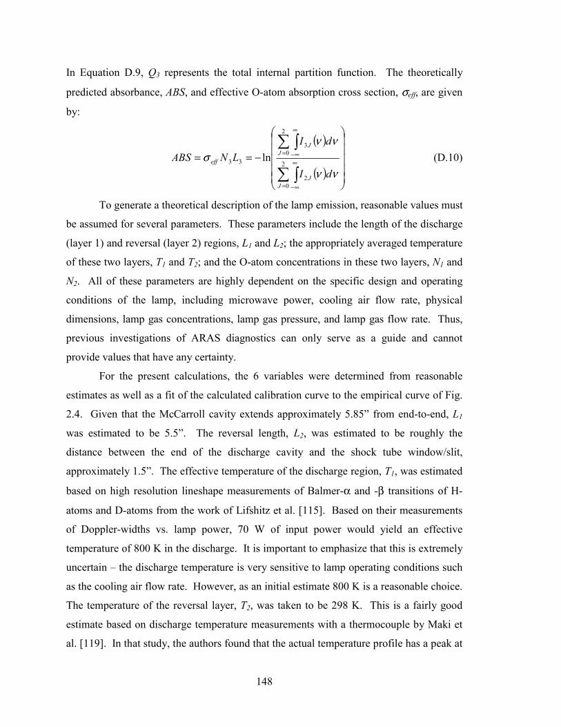
148

In Equation D.9, Q3 represents the total internal partition function. The theoretically

predicted absorbance, ABS, and effective O-atom absorption cross section, σeff, are given

by:

( )

( )

−==

∑ ∫

∑ ∫

=

∞

∞−

=

∞

∞−2

02

2

03

33 ln

JJ

JJ

eff

dI

dILNABS

νν

ννσ (D.10)

To generate a theoretical description of the lamp emission, reasonable values must

be assumed for several parameters. These parameters include the length of the discharge

(layer 1) and reversal (layer 2) regions, L1 and L2; the appropriately averaged temperature

of these two layers, T1 and T2; and the O-atom concentrations in these two layers, N1 and

N2. All of these parameters are highly dependent on the specific design and operating

conditions of the lamp, including microwave power, cooling air flow rate, physical

dimensions, lamp gas concentrations, lamp gas pressure, and lamp gas flow rate. Thus,

previous investigations of ARAS diagnostics can only serve as a guide and cannot

provide values that have any certainty.

For the present calculations, the 6 variables were determined from reasonable

estimates as well as a fit of the calculated calibration curve to the empirical curve of Fig.

2.4. Given that the McCarroll cavity extends approximately 5.85” from end-to-end, L1

was estimated to be 5.5”. The reversal length, L2, was estimated to be roughly the

distance between the end of the discharge cavity and the shock tube window/slit,

approximately 1.5”. The effective temperature of the discharge region, T1, was estimated

based on high resolution lineshape measurements of Balmer-α and -β transitions of H-

atoms and D-atoms from the work of Lifshitz et al. [115]. Based on their measurements

of Doppler-widths vs. lamp power, 70 W of input power would yield an effective

temperature of 800 K in the discharge. It is important to emphasize that this is extremely

uncertain – the discharge temperature is very sensitive to lamp operating conditions such

as the cooling air flow rate. However, as an initial estimate 800 K is a reasonable choice.

The temperature of the reversal layer, T2, was taken to be 298 K. This is a fairly good

estimate based on discharge temperature measurements with a thermocouple by Maki et

al. [119]. In that study, the authors found that the actual temperature profile has a peak at

149

the center of the discharge and decays to near room temperature on either end (Earlier

investigations of the two-layer model had assumed, for lack of better information, that T1

= T2).

Having set the first four parameters, the O-atom concentrations in layers 1 and 2

were adjusted in an attempt to best-fit the calibration curve given in Fig. 2.4. An

additional piece of information for this fitting process was the measurement of relative

intensities of the three multiplet components in Fig. D.1. Figure D.2 shows a close-up

view of the O-atom triplet lines. While the lineshapes cannot be fully resolved by our

monochromator, the relative peak intensities of the three transitions shown in Fig. D.2

will be directly proportional to the integrated intensity of the three transitions (since the

100 µm slits provide a 59 cm-1 bandwidth, and each transition has a linewidth of < 1

cm-1). At these lamp conditions, the three transitions are approximately equal in their

integrated intensities, with the J = 0 transition slightly lower than the other two.

The calibration curve was fit with the two-layer model by assuming shock tube

conditions of 2000 K and 1.2 atm (roughly the mean of the calibration experimental

conditions, ~1600-2400 K). The O-atom mole fractions giving a reasonable fit to the

initial part of the curve were X1 = 0.002 and X2 = 0.0001, indicating that roughly 10% of

the O2 dissociates in the lamp and only 1/20 of the resulting O-atoms diffuse into the

reversal layer. Given that much is unknown about the real lamp parameters, these O-

atom numbers are acceptable for the moment. The fit is shown in Fig. D.3. Comparing

the effective absorption cross sections from the empirical curve and the calculated curve,

the values agree within 2.5% up to ABS = 1.0, and within 10% up to ABS = 1.25. The

fitted O-atom concentrations also provide excellent agreement for the modeled relative

integrated intensities of the multiplet transitions, in the ratio of 1.04:1.025:1 for J = 2,1,0.

Other assumptions, for example higher values of T2, produced relative integrated

intensities which did not match the measured spectrum in Fig. D.2.

Given these starting assumptions, it is possible to ask what the model predicts for

the temperature-dependence of the cross section over the range of conditions of interest.

The calibration curve was calculated again using the conditions 2400 K, 1.1 atm and

1600 K, 1.45 atm, and these curves are shown in Fig. D.3. Clearly, the agreement is poor

and the model prediction is even outside of the scatter of the experimental data. The

150

deviation from the data indicates that the model assumptions are not quite right – which

is not surprising, given the number of unknowns. In addition, highly reversed lamp

emission lineshapes (as certainly this is) will yield effective absorption cross sections

which are particularly sensitive to pressure broadened absorption lineshapes. While

pressure broadening has not been specifically investigated for O-atoms, a pressure-

sensitive absorption cross section has been measured for N-atoms [45]. The lack of

pressure-broadening in the lineshape model may be responsible for the deviation of the

2000 K fit at high ABS in Fig. D.3, but it also may have resulted in incorrect fit

parameters yielding incorrect temperature dependence in the model.

One benefit of the model is the capability to visualize the emission and absorption

lineshapes, in order to understand the cause of the fall-off of the absorption cross section

at high ABS. A diagram of the lamp and shock tube is provided in Fig. D.4, along with

the calculated relative lineshapes using the two-layer model fit parameters at 2000 K.

Specifically, the lineshapes for the J = 1 transition are provided, although the other two

transitions are very similar with slightly different amounts of reversal. It is evident from

Fig. D.4 that the reversal of the emission lineshape has the effect of moving the bulk of

the radiant intensity into the wings of the absorption lineshape, where the absorption

cross section is smaller. As the emission passes through the shock tube, it is again

preferentially absorbed in the center and the intensity peaks are pushed farther and farther

into the wings, where the absorption cross section gets smaller and smaller. Thus, the

integrated effective absorption cross section decreases as the absorbance in the shock

tube increases, producing the calibration curve given in Figs. 2.4 and D.3.

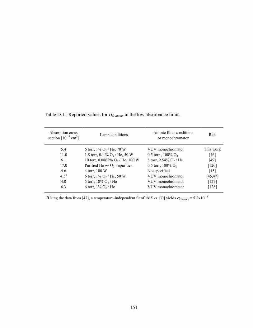
151

Table D.1: Reported values for σO-atoms in the low absorbance limit.

Absorption cross Atomic filter conditions section [10-15 cm2]

Lamp conditions or monochromator

Ref.

5.4 6 torr, 1% O2 / He, 70 W VUV monochromator This work 11.0 1.8 torr, 0.1 % O2 / He, 50 W 0.5 torr , 100% O2 [16] 6.1 10 torr, 0.0862% O2 / He, 100 W 8 torr, 9.54% O2 / He [49]

17.0 Purified He w/ O2 impurities 0.5 torr, 100% O2 [120] 4.6 4 torr, 100 W Not specified [15] 4.3a 6 torr, 1% O2 / He, 50 W VUV monochromator [45,47] 4.0 5 torr, 10% O2 / He VUV monochromator [127] 6.3 6 torr, 1% O2 / He VUV monochromator [128]

aUsing the data from [47], a temperature-independent fit of ABS vs. [O] yields σO-atoms = 5.2x10-15.

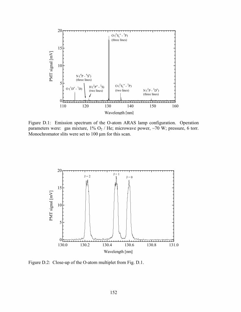
152

20

15

10

5

0

PMT

sign

al [m

V]

160150140130120110Wavelength [nm]

O (3S1o - 3P)

(three lines)

O (1Do - 1D)O (5S1

o - 3P)(two lines) N (2P - 2Do)

(three lines)

H (2Po - 2S)(two lines)

N (4P - 4So)(three lines)

Figure D.1: Emission spectrum of the O-atom ARAS lamp configuration. Operation parameters were: gas mixture, 1% O2 / He; microwave power, ~70 W; pressure, 6 torr. Monochromator slits were set to 100 µm for this scan.

20

15

10

5

0

PMT

sign

al [m

V]

131.0130.8130.6130.4130.2130.0Wavelength [nm]

J = 2J = 1

J = 0

Figure D.2: Close-up of the O-atom multiplet from Fig. D.1.

153

2.5

2.0

1.5

1.0

0.5

0.0

Abs

orba

nce

1086420

[O] 1013 atoms/cm3

Figure D.3: Experimental ARAS calibration curve compared to calculations using the two-layer model. Solid line and symbols: experimental data and polynomial fit; dashed line: model fit at 2000 K; dotted lines: model calculations for 1600 K and 2400 K using the same assumed lamp parameters.

Figure D.4: Effects of lamp self-absorption and line reversal on the emission lineshape.

1.5

0

Egamma1

11 deltanu1 0 1

0

1

1.5

0

Egamma1

11 deltanu1 0 1

0

1

Egamma1

deltanu1 0 1

0

1

Shock

Tube

Reversed lineshape Post-S.T. lineshape

1 10 13.

0

Line1

11 deltanu1 0 1

0

5 10 14

Self-absorbed lineshape

Relative emission

intensity

(ν – νo) [cm-1] (ν – νo) [cm-1] (ν – νo) [cm-1]

Absorption

cross section

(ν – νo) [cm-1]

155

Appendix E: The partial equilibrium of H2/O2 mixtures

E.1 The partial equilibrium hypothesis The partial equilibrium state achieved by H2/O2 mixtures in shock tube

experiments was first hypothesized by Schott [129] to explain the observed super-

equilibrium OH radical concentrations following the induction period and ignition. The

hypothesis is summarized in this appendix.

The overall reaction for hydrogen combustion is given by:

2H2 + O2 → 2H2O (E.1)

There are six major species participating in the combustion process, namely H2, O2, H, O,

OH, and H2O. Thermodynamic equilibrium considerations require two atom balance

relationships for H and O, and four independent reactions including one with a mole-

number change and therefore pressure-dependence. The mechanism associated with the

explosion limits and induction-time chemistry is:

H + O2 → OH + O (E.2)

O + H2 → OH + H (E.3)

OH + H2 → H2O + H (E.4)

As these three reactions are all mole-conserving, they alone cannot complete the

stoichiometry of Reaction (E.1), and recombination reactions must eventually take place.

At experimental conditions above the explosion limits, however, the OH production

through Reactions (E.2-E.4) is much faster than its removal by recombination reactions,

and it overshoots its final equilibrium concentration.

During the induction period, Reactions (E.3) and (E.4) are faster than Reaction

(E.2), and the O and OH radicals achieve a quasi-steady state while the H-atoms are

produced according to the stoichiometry (equal to E.2 + E.3 + 2xE.4):

156

3H2 + O2 = 2H2O + 2H (E.5)

As the initial reactants are depleted and OH, H, O, and H2O are formed in the post-

induction period, recombination reactions and the reverse of Reactions (E.2-E.4) will

become important. However, at high temperatures and low densities the recombination

process is often slow, and the dominant change in the reaction process becomes the

reversal of Reactions (E.2-E.4). Reactions (E.2-E.4) thus achieve equilibrium and the

concentrations of the species involved are related through the equilibrium constants of

these three reactions.

Two more equations can be written from Reactions (E.2-E.4) which, in addition

to Reaction (E.5), represent the stoichiometric formation of H, O, and OH from H2 and

O2:

H2 + O2 = H2O + O (E.6)

H2 + O2 = 2OH (E.7)

The equilibration of Equations (E.5-E.7) (which achieve equilibrium simultaneously with

Reactions (E.2-E.4)) is very rapid, and constantly keeps pace with any changes in

concentrations due to slow recombination processes. That is, these three reactions remain

in equilibrium even if some recombination occurs. However, if we further assume that

this process is so rapid that the bimolecular reactions reach equilibrium before any

recombination has occurred, we have reached a state of partial equilibrium of Reactions

(E.2-E.4) (or (E.5-E.7)) with no change in the mole number, n ≡ moles/total mass. Thus,

a stoichiometric condition can be written which balances the concentrations of the non-

diatomic species with the change in the total mole number:

( ) 0][][][][21

22 =

−−

−=− OHOHOHnn o

oo ρ

ρρ (E.8)

In this expression no, ρo, and [H2O]o are the initial mole number, density, and H2O

concentrations before any reaction occurs. Equations (E.5-E.8), along with the 2 atom

balances for H and O, define the partial equilibrium state. According the hypothesis by

Schott, this partial equilibrium state is a good approximation to the conditions at the OH

peak at high temperatures and low densities.

The benefit of the partial equilibrium hypothesis, if it holds true, is that the OH

peak concentrations at such experimental conditions are solely dependent on the

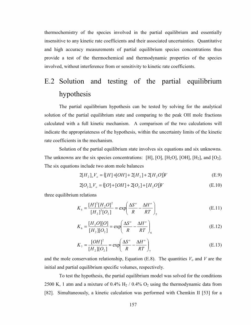
157

thermochemistry of the species involved in the partial equilibrium and essentially

insensitive to any kinetic rate coefficients and their associated uncertainties. Quantitative

and high accuracy measurements of partial equilibrium species concentrations thus

provide a test of the thermochemical and thermodynamic properties of the species

involved, without interference from or sensitivity to kinetic rate coefficients.

E.2 Solution and testing of the partial equilibrium

hypothesis The partial equilibrium hypothesis can be tested by solving for the analytical

solution of the partial equilibrium state and comparing to the peak OH mole fractions

calculated with a full kinetic mechanism. A comparison of the two calculations will

indicate the appropriateness of the hypothesis, within the uncertainty limits of the kinetic

rate coefficients in the mechanism.

Solution of the partial equilibrium state involves six equations and six unknowns.

The unknowns are the six species concentrations: [H], [O], [H2O], [OH], [H2], and [O2].

The six equations include two atom mole balances

( )VOHHOHHVH oo ][2][2][][][2 222 +++= (E.9)

( )VOHOOHOVO oo ][][2][][][2 222 +++= (E.10)

three equilibrium relations

52

32

22

2

5 exp][][][][

∆−∆==RTH

RS

OHOHHK

oo

(E.11)

622

26 exp

]][[]][[

∆−∆==RTH

RS

OHOOHK

oo

(E.12)

722

2

7 exp]][[

][

∆−∆==RTH

RS

OHOHK

oo

(E.13)

and the mole conservation relationship, Equation (E.8). The quantities Vo and V are the

initial and partial equilibrium specific volumes, respectively.

To test the hypothesis, the partial equilibrium model was solved for the conditions

2500 K, 1 atm and a mixture of 0.4% H2 / 0.4% O2 using the thermodynamic data from

[82]. Simultaneously, a kinetic calculation was performed with Chemkin II [53] for a

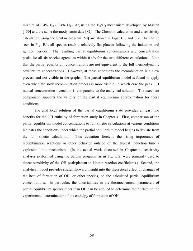
158

mixture of 0.4% H2 / 0.4% O2 / Ar, using the H2/O2 mechanism developed by Masten

[130] and the same thermodynamic data [82]. The Chemkin calculation and a sensitivity

calculation using the Senkin program [50] are shown in Figs. E.1 and E.2. As can be

seen in Fig. E.1, all species reach a relatively flat plateau following the induction and

ignition periods. The resulting partial equilibrium concentrations and concentration

peaks for all six species agreed to within 0.4% for the two different calculations. Note

that the partial equilibrium concentrations are not equivalent to the full thermodynamic

equilibrium concentrations. However, at these conditions the recombination is a slow

process and not visible in the graphs. The partial equilibrium model is found to apply

even when the slow recombination process is more visible, in which case the peak OH

radical concentration overshoot is comparable to the analytical solution. The excellent

comparison supports the validity of the partial equilibrium approximation for these

conditions.

The analytical solution of the partial equilibrium state provides at least two

benefits for the OH enthalpy of formation study in Chapter 4. First, comparison of the

partial equilibrium model concentrations to full kinetic calculations at various conditions

indicates the conditions under which the partial equilibrium model begins to deviate from

the full kinetic calculation. This deviation foretells the rising importance of

recombination reactions or other behavior outside of the typical induction time /

explosion limit mechanism. (In the actual work discussed in Chapter 4, sensitivity

analyses performed using the Senkin program, as in Fig. E.2, were primarily used to

detect sensitivity of the OH peak/plateau to kinetic reaction coefficients.) Second, the

analytical model provides straightforward insight into the theoretical effect of changes of

the heat of formation of OH, or other species, on the calculated partial equilibrium

concentrations. In particular, the uncertainties in the thermochemical parameters of

partial equilibrium species other than OH can be applied to determine their effect on the

experimental determination of the enthalpy of formation of OH.

159

0 50 100 150 200 250 300

0

500

1000

1500

2000

2500

3000

3500

4000

4500

Spec

ies m

ole

frac

tion

[ppm

]

Time [µs]

H2 O2

H H2O O OH

Partial equilibrium

Figure E.1: Chemkin calculation for comparison to the partial equilibrium model. Conditions are 2500 K, 1 atm with a mixture of 0.4% H2 / 0.4% O2 / Ar. Mechanism is from Masten [130] and thermodynamic data from Kee et al. [82].

0 50 100 150 200 250 300-0.2

0.0

0.2

0.4

0.6

0.8

1.0

1.2

1.4

OH

Sen

sitiv

ity

Time [µs]

H + O2 = OH + O

O + H2 = OH + H

OH + H2 = H2O + H H

2 + O

2 = H + HO

2

H2 + M = 2H + M

2OH = O + H2O H + O

2 + M = HO

2 + M

Insensitive to kinetics

Figure E.2: Sensitivity calculations for the conditions of Fig. E.1.

161

References

[1] R. Zhu, C.C. Hsu, and M.C. Lin, "Ab initio study of the CH3+O2 reaction: Kinetics,

mechanism and product branching probabilities," J. Chem. Phys. 115 (1) (2001)

195-203.

[2] A.C. Baldwin and D.M. Golden, "Reactions of methyl radicals of importance in

combustion systems," Chem. Phys. Let. 55 (2) (1978) 350-352.

[3] K.A. Bhaskaran, P. Frank, and T. Just, "High temperature methyl radical reactions

with atomic and molecular oxygen," Shock Tubes and Waves, Proceedings of the

Twelfth International Symposium on Shock Tubes and Waves, Jerusalem, Israel

(1979), Magnes Press, Jerusalem, 1980, p. 503-513.

[4] A.A. Borisov, E.V. Dragalova, V.M. Zamanskii, V.V. Lisyanskii, and G.I. Skachkov,

"Mechanism for the combustion of methane-oxygen mixtures in the presence of

added N2O," Kinet. Katal. 22 (2) (1981) 305-311.

[5] C.T. Bowman, "Non-equilibrium radical concentrations in shock-initiated methane

oxidation," Proc. Combust. Inst. 15 (1975) 869-882.

[6] T.A. Brabbs and R.S. Brokaw, "Shock tube measurements of specific reaction rates in

the branched chain CH4-CO-O2 system," Proc. Combust. Inst. 15 (1975) 893-901.

[7] M. Braun-Unkhoff, C. Naumann, and P. Frank, "A shock tube study of the reaction

CH3+O2," Shock Waves @ Marseille, Proceedings of the 19th International

Symposium on Shock Waves, Marseille, France (1993), Springer-Verlag, Berlin,

1995, p. 203-208.

[8] T.C. Clark, T.P.J. Izod, and S. Matsuda, "Oxidation of methyl radicals studied in

reflected shock waves using the time-of-flight mass spectrometer," J. Chem. Phys.

55 (9) (1971) 4644-4647.

[9] A.M. Dean and G.B. Kistiakowsky, "Oxidation of carbon monoxide/methane

mixtures in shock waves," J. Chem. Phys. 54 (4) (1971) 1718-1725.

162

[10] M.A. Grela, V.T. Amorebieta, and A.J. Colussi, "High-temperature oxidation of

methyl radicals in open systems," J. Phys. Chem. 96 (17) (1992) 7013-7018.

[11] D.S.Y. Hsu, W.M. Shaub, T. Creamer, D. Gutman, and M.C. Lin, "Kinetic modeling

of CO production from the reaction of CH3 with O2 in shock waves," Ber.

Bunsenges. Phys. Chem. 87 (10) (1983) 909-919.

[12] S.M. Hwang, S.O. Ryu, K.J. De Witt, and M.J. Rabinowitz, "Rate coefficient

measurements of the reaction CH3+O2 = CH3O+O," J. Phys. Chem. A 103 (30)

(1999) 5949-5958.

[13] T.P.J. Izod, G.B. Kistiakowsky, and S. Matsuda, "Oxidation of carbon monoxide

mixtures with added ethane or azomethane studied in incident shock waves," J.

Chem. Phys. 55 (9) (1971) 4425-4432.

[14] C.J. Jachimowski, "Kinetics of oxygen atom formation during the oxidation of

methane behind shock waves," Combust. Flame 23 (2) (1974) 233-248.

[15] M. Klatt, M. Rohrig, and H.G. Wagner, "An investigation of the reaction of CH3

radicals with O2 at high temperatures," Ber. Bunsenges. Phys. Chem. 95 (10)

(1991) 1163-1168.

[16] J.V. Michael, S.S. Kumaran, and M.C. Su, "Rate constants for CH3+O2 → CH3O+O

at high temperature and evidence for H2CO+O2 → HCO+HO2," J. Phys. Chem. A

103 (30) (1999) 5942-5948.

[17] K. Ohmori, M. Yoshimura, M. Koshi, and H. Matsui, "A flash photolysis study of

CH4-O2 mixtures behind shock waves: Examination of reaction of CH3+O2," Bull.

Chem. Soc. Japan 65 (5) (1992) 1317-1322.

[18] D.B. Olson and W.C. Gardiner Jr., "Combustion of methane in fuel-rich mixtures,"

Combust. Flame 32 (2) (1978) 151-161.

[19] K. Saito, R. Ito, T. Kakumoto, and A. Imamura, "The initial process of the oxidation

of the methyl radical in reflected shock waves," J. Phys. Chem. 90 (7) (1986)

1422-1427.

[20] J.J. Scire Jr., R.A. Yetter, and F.L. Dryer, "Flow reactor studies of methyl radical

oxidation reactions in methane-perturbed moist carbon monoxide oxidation at

high pressure with model sensitivity analysis," Int. J. Chem. Kinet. 33 (2) (2001)

75-100.

163

[21] K. Tabayashi and S.H. Bauer, "The early stages of pyrolysis and oxidation of

methane," Combust. Flame 34 (1) (1979) 63-83.

[22] T. Tsuboi, "Mechanism for homogeneous thermal oxidation of methane in gas

phase," Japan. J. App. Phys. 15 (1) (1976) 159-168.

[23] C.H. Wu, C.-Y. Lin, and H.-T. Wang, "A shock tube study of the oxidation of the

methyl radical," Current Topics in Shock Waves, 17th International Symposium

on Shock Waves & Shock Tubes, Bethlehem (1989), American Institute of Physics,

New York, 1990, p. 450-455.

[24] C.L. Yu, C. Wang, and M. Frenklach, "Chemical kinetics of methyl oxidation by

molecular oxygen," J. Phys. Chem. 99 (39) (1995) 14377-14387.

[25] A.M. Dean and P.R. Westmoreland, "Bimolecular QRRK analysis of methyl radical

reactions," Int. J. Chem. Kinet. 19 (3) (1987) 207-228.

[26] M.A. Teitelboim, L.B. Romanovich, and V.I. Vedeneev, "RRKM theoretical

calculation of some reaction channels of the methyl radical with oxygen," Kinet.

Katal. 19 (6) (1978) 1399-1404.

[27] R. Zellner and F. Ewig, "Computational study of the CH3 + O2 chain branching

reaction," J. Phys. Chem. 92 (10) (1988) 2971-2974.

[28] A. Burcat and W.C. Gardiner Jr, "Thermochemistry," in: W. Gardiner Jr (Ed.), Gas-

Phase Combustion Chemistry. Springer-Verlag, New York, 1999, p. 497.

[29] B. Ruscic, D. Feller, D.A. Dixon, K.A. Peterson, L.B. Harding, R.L. Asher, and A.F.

Wagner, "Evidence for a lower enthalpy of formation of hydroxyl radical and a

lower gas-phase bond dissociation energy of water," J. Phys. Chem. A 105 (1)

(2001) 1-4.

[30] B. Ruscic, A.F. Wagner, L.B. Harding, R.L. Asher, D. Feller, D.A. Dixon, K.A.

Peterson, Y. Song, X. Qian, C.Y. Ng, J. Liu, W. Chen, and D.W. Schwenke, "On

the enthalpy of formation of hydroxyl radical and gas-phase bond dissociation

energies of water and hydroxyl," J. Phys. Chem. A 106 (11) (2002) 2727-2747.

[31] L.V. Gurvich, I.V. Veyts, and C.B. Alcock (Ed.), Thermodynamic Properties of

Individual Substances (4th ed.) Vol. I, Parts 1 & 2. Hemisphere, New York, 1989.

[32] M.W. Chase Jr., NIST-JANAF Thermochemical Tables. American Chemical Society

and American Physical Society, Washington, 1998.

164

[33] R.T. Birge and H. Sponer, "The heat of dissociation of non-polar molecules," Phys.

Rev. 28 (2) (1926) 259-283.

[34] C. Carlone and F.W. Dalby, "Spectrum of the hydroxyl radical," Can. J. Phys. 47

(18) (1969) 1945-1958.

[35] J.A. Joens, "The dissociation energy of OH(X2Π3/2) and the enthalpy of formation of

OH(X2Π3/2), ClOH, and BrOH from thermochemical cycles," J. Phys. Chem. A

105 (49) (2001) 11041-11044.

[36] E.J. Chang, Shock Tube Experiments for the Development and Validation of Models

of Hydrocarbon Combustion, Mechanical Engineering, Stanford University,

Engineer's Thesis 1995, 101 pages.

[37] G.P. Smith, D.M. Golden, M. Frenklach, N.W. Moriarty, B. Eiteneer, M.

Goldenberg, C.T. Bowman, R.K. Hanson, S. Song, W.C. Gardiner Jr., V.V.

Lissianski, and Z. Qin, GRI-Mech 3.0, www.me.berkeley.edu/gri_mech/, Gas

Research Institute, 2000.

[38] R.K. Hanson, S. Salimian, G. Kychakoff, and R.A. Booman, "Shock-tube absorption

measurements of OH using a remotely located dye laser," Appl. Optics 22 (5)

(1983) 641-643.

[39] E.C. Rea Jr., A.Y. Chang, and R.K. Hanson, "Shock-tube study of pressure

broadening of the A2Σ+-X2Π(0,0) band of OH by Ar and N2," JQSRT 37 (2)

(1987) 117-127.

[40] E.C. Rea Jr., S. Salimian, and R.K. Hanson, "Rapid-tuning frequency-doubled ring

dye-laser for high-resolution absorption-spectroscopy in shock-heated gases,"

Appl. Optics 23 (11) (1984) 1691-1694.

[41] E.L. Petersen, A Shock Tube and Diagnostics for Chemistry Measurements at

Elevated Pressures with Application to Methane Ignition, Mechanical

Engineering, Stanford University, Ph.D. 1998, 364 pages.

[42] WA-1000 and WA-1500 Wavemeter Operating Manual, 06737-M-00, Rev. C,

Burleigh Instruments, Inc., 1995.

[43] D.F. Davidson and R.K. Hanson, "Measurement techniques and diagnostics," in: G.

Ben-Dor, O. Igra T. Elperin (Ed.), Handbook of Shock Waves, Vol. 1: Theoretical,

http://www.me.berkeley.edu/gri_mech/

165

Experimental, and Numerical Techniques. Academic Press, San Diego, 2001, p.

766-770.

[44] J.V. Michael and A. Lifshitz, "Atomic resonance absorption spectroscopy with flash

or laser photolysis in shock wave experiments," in: G. Ben-Dor, O. Igra T.

Elperin (Ed.), Handbook of Shock Waves, Vol. 3: Chemical Reactions in Shock

Waves and Detonations. Academic Press, San Diego, 2001, p. 77-90.

[45] D.F. Davidson and R.K. Hanson, "High-temperature reaction rate coefficients

devired from N-atom ARAS measurements and excimer photolysis," Int. J. Chem.

Kinet. 22 (8) (1990) 843-861.

[46] A.J. Dean, R.K. Hanson, and C.T. Bowman, "A shock tube study of reactions of C

atoms and CH with NO including product channel measurements," J. Phys. Chem.

95 (8) (1991) 3180-3189.

[47] A.J. Dean, A Shock Tube Study of NOx Reactions Involving CH and C-atoms Using

Laser and Atomic Resonance Absorption Diagnostics, Mechanical Engineering,

Stanford University, Ph.D. 1990, 217 pages.

[48] B. McCarroll, "An improved microwave discharge cavity for 2450 MHz," Rev. Sci.

Inst. 41 (2) (1970) 279-280.

[49] S.K. Ross, J.W. Sutherland, S.C. Kuo, and R.B. Klemm, "Rate constants for the

thermal dissociation of N2O and the O(P3)+N2O reaction," J. Phys. Chem. A 101

(6) (1997) 1104-1116.

[50] A.E. Lutz, R.J. Kee, and J.A. Miller, Senkin: A FORTRAN program for predicting

homogeneous gas phase chemical kinetics with sensitivity analysis, Report No.

SAND87-8248, Sandia National Laboratories, 1988.

[51] R.C. Millikan and D.R. White, "Systematics of vibrational relaxation," J. Chem.

Phys. 39 (12) (1963) 3209-3213.

[52] K. Takahashi, A. Inoue, and T. Inomata, "Direct measurements of rate coefficients

for thermal decomposition of methyl halides using shock-tube ARAS technique,"

Proceedings of the 20th International Symposium on Shock Waves, Pasadena

(1995), World Scientific, Singapore, 1996, p. 959-964.

166

[53] R.J. Kee, F.M. Rupley, and J.A. Miller, Chemkin II: A FORTRAN chemical kinetics

package for the analysis of gas-phase chemical kinetics, Report No. SAND-89-

8009, Sandia National Laboratories, 1989.

[54] D.M. Golden and J.A. Manion, "Applications of chemical kinetics," Advances in

Chemical Kinetics and Dynamics 1 (1992) 187-276.

[55] B. Eiteneer and M. Frenklach, "Comment on "Rate constants for CH3+O2 →

CH3O+O at high temperature and evidence for H2CO+O2 → HCO+HO2" and

"Rate coefficient measurements of the reaction CH3+O2 = CH3O+O"," J. Phys.

Chem. A 104 (43) (2000) 9797-9799.

[56] J.V. Michael, S.S. Kumaran, and M.C. Su, "Reply to Comment on "Rate constants

for CH3+O2 → CH3O+O at high temperature and evidence for H2CO+O2 →

HCO+HO2"," J. Phys. Chem. A 104 (43) (2000) 9800-9802.

[57] S.M. Hwang, S.O. Ryu, K.J. Dewitt, and M.J. Rabinowitz, "Reply to the comment

on " Rate coefficient measurements of the reaction CH3+O2 = CH3O+O "," J.

Phys. Chem. A 104 (43) (2000) 9803-9805.

[58] J.V. Michael, "Rate constants for the reaction O+D2→OD+D by the flash

photolysis-shock tube technique over the temperature range 825-2487K: The H2

to D2 isotope effect," J. Chem. Phys. 90 (1) (1989) 189-198.

[59] J.V. Michael, "Measurement of thermal rate constants by flash or laser photolysis in

shock-tubes – oxidations of H2 and D2," Prog. Energy Combust. Sci. 18 (4) (1992)

327-347.

[60] W. Tsang, "Heats of formation of organic free radicals by kinetic methods," in: J.A.

Martinho Simones, A. Greenberg J.F. Liebman (Ed.), Energetics of Organic Free

Radicals. Blackie Academic and Professional, London, 1996, p. 22-58.

[61] R.S. Figliola and D.E. Beasley, Theory and Design for Mechanical Measurements.

John Wiley & Sons, Inc., New York, 1995.

[62] D.L. Baulch et al., "Evaluated kinetic data for combustion modeling," submitted to J.

Phys. Chem. Ref. Data (2004).

[63] G. Friedrichs, D.F. Davidson, and R.K. Hanson, "Validation of a thermal

decomposition mechanism of formaldehyde by detection of CH2O and HCO

behind shock waves," Int. J. Chem. Kinet. 36 (3) (2004) 157-169.

167

[64] G. Friedrichs, J.T. Herbon, D.F. Davidson, and R.K. Hanson, "Quantitative detection

of HCO behind shock waves: The thermal decomposition of HCO," Phys. Chem.

Chem. Phys. 4 (23) (2002) 5778-5788.

[65] R.W. Bates, D.M. Golden, R.K. Hanson, and C.T. Bowman, "Experimental study

and modeling of the reaction H+O2+M→HO2+M (M=Ar, N2, H2O) at elevated

pressures and temperatures between 1050 and 1250 K," Phys. Chem. Chem. Phys.

3 (12) (2001) 2337-2342.

[66] V. Vasudevan, in preparation, (2004)

[67] H. Hippler, H. Neunaber, and J. Troe, "Shock wave studies of the reactions

HO+H2O2→H2O+HO2 and HO+HO2→H2O+O2 between 930 and 1680K," J.

Chem. Phys. 103 (9) (1995) 3510-3516.

[68] T. Hidaka, T. Taniguchi, H. Tanaka, T. Kamesawa, K. Inami, and H. Kawano,

"Shock-tube study of CH2O pyrolysis and oxidation," Combust. Flame 92 (4)

(1993) 365-376.

[69] R.R. Baldwin, A.R. Fuller, D. Longthorn, and R.W. Walker, "Oxidation of

formaldehyde in KCl-coated vessels," Journal of the Chemical Society-Faraday

Transactions I 70 (7) (1974) 1257-1268.

[70] J.V. Michael, M.C. Su, J.W. Sutherland, D.C. Fang, L.B. Harding, and A.F. Wagner,

"Rate constants for H2CO+O2→HCO+HO2 at high temperature,” Abstract 4-B03,

Work in Progress Posters, 28th Symp. (Int.) Combust., Edinburgh, Scotland

(2000), p. 361.

[71] J.T. Herbon and R.K. Hanson, "Measurement of collision-shift in absorption

transitions of the OH A-X(0,0) band using a shock tube," Proceedings of the

Twenty-Third International Symposium on Shock Waves, Fort Worth (2001), p.

557-564.

[72] A. Goldman and J.R. Gillis, "Spectral line parameters for the A2Σ-X2Π(0,0) band of

OH for atmospheric and high-temperatures," JQSRT 25 (2) (1981) 111-135.

[73] G. Stark, J.W. Brault, and M.C. Abrams, "Fourier-transform spectra of the A2Σ+-

X2Π ∆v = 0 bands of OH and OD," J OPT SOC B 11 (1) (1994) 3-32.

[74] J.R. Gillis, A. Goldman, G. Stark, and C.P. Rinsland, "Line parameters for the A2Σ+-

X2Π bands of OH," JQSRT 68 (2) (2001) 225-230.

168

[75] J. Luque and D.R. Crosley, "Transition probabilities in the A2Σ+-X2Πi electronic

system of OH," J. Chem. Phys. 109 (2) (1998) 439-448.

[76] K.R. German, "Direct measurement of the radiative lifetimes of the A2Σ+ (v' = 0)

states of OH and OD," J. Chem. Phys. 62 (7) (1975) 2584-2587.

[77] J. Luque and D.R. Crosley, LIFBASE: Database and spectral simulation program

(Version 1.6), Report No. MP 99-009, SRI International, 1999.

[78] G. Herzberg, Molecular Spectra and Molecular Structure, Vol. I: Spectra of

Diatomic Molecules. Van Nostrand, Princeton, 1950.

[79] K.P. Huber and G. Herzberg, Molecular Spectra and Molecular Structure, Vol. IV:

Constants of Diatomic Molecules. Reinhold, New York, 1979.

[80] A. Burcat, "Thermochemical data for combustion calculations," in: W.C. Gardiner Jr

(Ed.), Combustion Chemistry. Springer-Verlag, New York, 1984, p. 455-504.

[81] D.L. Baulch, C.J. Cobos, R.A. Cox, C. Esser, P. Frank, T. Just, J.A. Kerr, M.J.

Pilling, J. Troe, R.W. Walker, and J. Warnatz, "Evaluated kinetic data for

combustion modeling," J. Phys. Chem. Ref. Data 21 (3) (1992) 411-734.

[82] R.J. Kee, F.M. Rupley, and J.A. Miller, The CHEMKIN thermodynamics data base,

Report No. SAND87-8215B, Sandia National Laboratories, 1987.

[83] A. Burcat, Third millenium ideal gas and condensed phase thermochemical

database for combustion, Report No. TAE 867, Technion, Israel Institute of

Technology, 2001.

[84] A. Burcat, personal communication, October 2001.

[85] W.L. Dimpfl and J.L. Kinsey, "Radiative lifetimes of OH(A2Σ) and Einstein

coefficients for the A-X system of OH and OD," JQSRT 21 (3) (1979) 233-241.

[86] M. Thoma, R. Kaschow, and F. Hindelang, "A multiple-reflection cell suited for

absorption measurements in shock tubes," Shock Waves 4 (1) (1994) 51-53.

[87] M.C. Su, S.S. Kumaran, K.P. Lim, and J.V. Michael, "Multipass optical detection in

reflected shock waves: Application to OH radicals," Rev. Sci. Inst. 66 (9) (1995)

4649-4654.

[88] S.M. Chernin, "Multipass annular mirror system for spectroscopic studies in shock

tubes," J. Modern Opt. 51 (2) (2004) 223-231.

169

[89] D.S. Baer, J.B. Paul, M. Gupta, and A. O'Keefe, "Sensitive absorption measurements

in the near-infrared region using off-axis integrated-cavity-output spectroscopy,"

App. Phys. B 75 (2-3) (2002) 1-6.

[90] G. Friedrichs and H.G. Wagner, "Quantitative fm spectroscopy at high temperatures:

The detection of 1CH2 behind shock waves," Z. Phys. Chem. 214 (12) (2000)

1723-1746.

[91] J. Deppe, G. Friedrichs, H.-J. Romming, A. Ibrahim, and H.G. Wagner, "The

thermal decomposition of NH2 and NH radicals," Ber. Bunsenges. Phys. Chem.

102 (10) (1998) 1474-1485.

[92] M. Votsmeier, S. Song, D.F. Davidson, and R.K. Hanson, "Sensitive detection of

NH2 in shock tube experiments using frequency modulation spectroscopy," Int. J.

Chem. Kinet. 31 (6) (1999) 445-453.

[93] M. Frenklach, H. Wang, and M.J. Rabinowitz, "Optimization and analysis of large

chemical kinetic mechanisms using the solution mapping method – combustion of

methane," Prog. Energy Combust. Sci. 18 (1) (1992) 47-73.

[94] G.H. Dieke and H.M. Crosswhite, "The ultraviolet bands of OH – fundamental

data," JQSRT 2 (2) (1962) 97-199.

[95] E.C. Rea Jr, Rapid-Tuning Laser Wavelength Modulation Spectroscopy with

Applications in Combustion Diagnostics and OH Line Shape Studies, Mechanical

Engineering, Stanford University, Ph.D. 1991, 369 pages.

[96] I.L. Chidsey and D.R. Crosley, Tables of calculated transition probabilities for the

A-X system of OH, Report No. ARBRL-TR-0326, Ballistic Research Laboratory,

1981.

[97] J.A. Coxon, "Optimum molecular constants and term values for the X2Π (v ≤ 5) and

A2Σ+ (v ≤ 3) states of OH," Can. J. Phys. 58 (7) (1980) 933-949.

[98] W.G. Vincenti and C.H. Kruger Jr., Introduction to Gas Dynamics. Krieger, Malabar,

1959.

[99] A. Goldman, personal communication, 2001.

[100] F. Melen, A.J. Sauval, N. Grevesse, C.B. Farmer, C. Servais, L. Delbouille, and G.

Roland, "A new analysis of the OH radical spectrum from solar infrared

observations," J. Molec. Spec. 174 (2) (1995) 490-509.

170

[101] A. Goldman, "Line parameters for the atmospheric band system of OH," Appl.

Optics 21 (12) (1982) 2100-2102.

[102] J.A. Coxon and S.C. Foster, "Rotational analysis of hydroxyl vibration-rotation

emission bands: Molecular constants for OH X2Π, 6 ≤ v ≤ 10," Can. J. Phys. 60

(1) (1982) 41-48.

[103] C.C. Wang, D.K. Killinger, and C.M. Huang, "Rotational dependence in the

linewidth of the ultraviolet transitions of OH," Phys. Rev. A 22 (1) (1980) 188-

191.

[104] B. Shirinzadeh, D.M. Bakalyar, and C.C. Wang, "Measurement of collision-

induced shift and broadening of the ultraviolet transitions of OH," J. Chem. Phys.

82 (7) (1985) 2877-2879.

[105] E.C. Rea Jr, A.Y. Chang, and R.K. Hanson, "Collisional broadening of the A2Σ+-

X2Π (0,0) band of OH by H2O and CO2 in atmospheric-pressure flames," JQSRT

41 (1) (1989) 29-42.

[106] D.F. Davidson, M. Rohrig, E.L. Petersen, M.D. Di Rosa, and R.K. Hanson,

"Measurements of the OH A-X(0,0) 306nm absorption bandhead at 60 atm and

1735 K," JQSRT 55 (6) (1996) 755-762.

[107] W.J. Kessler, M.G. Allen, and S.J. Davis, "Rotational level-dependent collisional

broadening and line shift of the A2Σ+ - X2Π (1,0) band of OH in hydrogen-air

combustion gases," JQSRT 49 (2) (1993) 107-117.

[108] A.Y. Chang, Rapid-Tuning Continuous-Wave Laser Technique Applied to Nitric

Oxide Spectroscopy and Flow Measurements, Mechanical Engineering, Stanford

University, Ph.D. 1991, 232 pages.

[109] P.L. Varghese and R.K. Hanson, "Collisional narrowing effects on spectral ine

shapes measured at high resolution," Appl. Optics 23 (14) (1984) 2376-2385.

[110] A.G. Gaydon and I.R. Hurle, The Shock Tube in High-Temperature Chemical

Physics. Reinhold, New York, 1963.

[111] P.R. Bevington and D.K. Robinson, Data Reduction and Error Analysis for the

Physical Sciences. McGraw-Hill, New York, 1992.

[112] W. Braun and T. Carrington, "Line emission sources for concentration

measurements and photochemistry," JQSRT 9 (8) (1969) 1133-1143.

171

[113] A.C.G. Mitchell and M.W. Zemansky, Resonance Radiation and Excited Atoms.

Cambridge University Press, London, 1934.

[114] W. Braun, A.M. Bass, and D.D. Davis, "Experimental test of a two-layer model

characterizing emission-line profiles," Journal of the Optical Society of America

60 (2) (1970) 166-170.

[115] A. Lifshitz, G.B. Skinner, and D.R. Wood, "Resonance absorption measurements

of atom concentrations in reacting gas mixtures. I. Shapes of H and D Lyman-α

lines from microwave sources," J. Chem. Phys. 70 (12) (1979) 5607-5613.

[116] K.M. Pamidimukkala, A. Lifshitz, G.B. Skinner, and D.R. Wood, "Resonance

absorption measurements of atom concentrations in reacting gas mixtures. VI.

Shapes of the vacuum ultraviolet oxygen (3S-3P) resonance triplet from

microwave sources and empirical calibration in a shock tube," J. Chem. Phys. 75

(3) (1981) 1116-1122.

[117] K.P. Lynch, T.C. Schwab, and J.V. Michael, "Lyman-α absorption photometry at

high pressure and atom density kinetic results for H recombination," Int. J. Chem.

Kinet. 8 (5) (1976) 651-671.

[118] C.-C. Chiang, A. Lifshitz, G.B. Skinner, and D.R. Wood, "Resonance absorption

measurements of atom concentrations in reacting gas mixtures. II. Calibration of

microwave sources over a wide temperature range," J. Chem. Phys. 70 (12)

(1979) 5614-5622.

[119] R.G. Maki, J.V. Michael, and J.W. Sutherland, "Lyman-α photometry: Curve of

growth determination, comparison to theoretical oscillator strength, and line

absorption calculations at high temperature," J. Phys. Chem. 89 (22) (1985) 4815-

4821.

[120] J.V. Michael and K.P. Lim, "Rate constants for the N2O reaction system – thermal

decomposition of N2O, N+NO→N2+O and implications for O+N2→NO+N," J.

Chem. Phys. 97 (5) (1992) 3228-3234.

[121] J.H. Lee, J.V. Michael, W.A. Payne, and L.J. Stief, "Absolute rate of the reaction of

N(4S) with NO from 196-400 K with DF-RF and FP-RF techniques," J. Chem.

Phys. 69 (7) (1978) 3069-3076.

172

[122] J.W. Sutherland, J.V. Michael, and R.B. Klemm, "Rate constant for the O(3P) +

CH4 → OH + CH3 reaction obtained by the flash photolysis-shock tube technique

over the temperature range 763 ≤ T ≤ 1755 K," J. Phys. Chem. 90 (22) (1986)

5941-5945.

[123] P.M. Patterson, J.W. Sutherland, and R.B. Klemm, "High temperature study of the

reaction of O(3P) + NH3," Current Topics in Shock Waves, 17th International

Symposium on Shock Waves & Shock Tubes, Bethlehem (1990), American

Institute of Physics, New York, 1990, p. 444-449.

[124] A. Lifshitz, G.B. Skinner, and D.R. Wood, "Improved high-intensity microwave

discharge lamp for atomic resonance absorption and fluorescence spectroscopy,"

Rev. Sci. Inst. 49 (9) (1978) 1322-1323.

[125] D. Davis and W. Braun, "Intense vacuum ultraviolet atomic line sources," Appl.

Optics 7 (10) (1968) 2071-2074.

[126] F.C. Fehsenfeld, K.M. Evenson, and H.P. Broida, "Microwave discharge cavities

operating at 2450 MHz," Rev. Sci. Inst. 36 (3) (1965) 294-298.

[127] N. Fujii, N.F. Sagawai, T. Sato, Y. Nosaka, and H. Miyama, "Study of the thermal

dissociation of N2O and CO2 using O(3P) atomic resonance absorption

spectroscopy," J. Phys. Chem. 93 (14) (1989) 5474-5478.

[128] K. Thielen and P. Roth, "Resonance absorption measurements of N and O atoms in

high temperature NO dissociation and formation kinetics," Proc. Combust. Inst.

20 (1984) 685-693.

[129] G.L. Schott, "Kinetic studies of hydroxyl radicals in shock waves. III. The OH

concentration maximum in the hydrogen-oxygen reaction," J. Chem. Phys. 32 (3)

(1960) 710-716.

[130] D.A. Masten, A Shock Tube Study of Reactions in the H2/O2 Mechanism, Mechanical Engineering, Stanford University, Ph.D. 1990, 138 pages.

shock tube measurements of ch3+o2 kinetics and the heat …

Documents