:. ...............:_:/.._ ......:_ f%;i:_.........12;............_,:'_,/._ii"S-i:i'_/_"%'_........i i 206 3 59

....... _ ,_

,_7""i L,..s;;,.+'_'_+_"

.<, /

/.l' f:' 11

SIGNAL-PROCESSING ALGORITHM

DEVELOPMENT FOR THE ACLAIM SENSOR

Final Report: Gust Detection

prepared for

NASA Dryden Flight Research Center

ACLAIM program

under

Cooperative Agreement No. NCC4-0014

Alabama A&M University

Office of Research and Development

Normal, Alabama35762-0411

https://ntrs.nasa.gov/search.jsp?R=19980002723 2018-08-27T10:32:59+00:00Z

Table of Contents

Empirical Orthonormal Functions .................... 4

Conclusions 13OOOOOOOOOOOOOOOOOOOOOOOOOOOOOOOOOOOOOOOOOOOOOOOOOOOO

SIGNAL-PROCESSING ALGORITHM

DEVELOPMENT FOR THE ACLAIM SENSOR

Final Report: Gust Detection

Scott yon Laven

Introduction

As described in previous ACLAIM reports 1-2, the ACLAIM program is a demonstration

of the feasibility of using an on-board look-ahead lidar to measure wind velocities.

Indications are that such a lidar has sufficient range to prevent engine unstart in aircraft

such as the High-Speed Civil Transport (HSCT). A change in Mach number of

approximately five per cent is considered sufficient to cause unstart if it occurs on a time

scale of seconds or less, as shown in Fig. 13.

_Z• 0.2

_015 -,E O.I

_005gIP&.Ig

0

, 0.25--

I I I I

0 2 4 6 8

duration of gust (seconds}

Fig. 1. Gust magnitude required to cause unstart.

Our general approach to improving the detection of wind-field disturbances, such as a

sudden change in Mach number, is, first, to attempt to determine characteristic patterns is

the wind field and, second, to use that information to evaluate the probability that partial

events might grow into full events (Fig. 2). Throughout this report wind-field

disturbances may also be referred to as "events", or in some circumstances "gusts".

m

mm

oo-

/

w,

/

/

/

//

s

/

/

\

\

I

i

\

\

\

\

i

\\

\

I I --f - I

time

Fig. 2. An example of a signal (circles), referred to as a partial event or precursor) that

might indicate a significant wind-field event or gust (dashes).

In consultation with other ACLAIM participants, a detailed approach involving empirical

orthonormal functions (EOFs) was pursued and is summarized in the next section. In the

subsequent section we describe wind-field simulations that show how an event-detection

scheme employing partial events (precursors) might be calibrated.

Empirical Orthonormal Functions

EOF's are eigenfimctions (%) obtained from an arbitrary data set by solving the

eigenvalue equation associated with data set's two-point correlation function (K).

Expli citly we solve

n(x)dx - (y)(1)

for the first few On, where the 7,n are the eigenvalues and

K(x, y)- (f (x) f (y)) (2)

and x and y both refer to time (or, equivalently, the axial coordinate). References 4 and 5

discuss EOFs in a context similar to ACLAIM.

The example presented in Figures 3 and 4 illustrates the concept of EOFs.

400 --

300 -

200 "

100-

O-T

-100--- 0_1 CO _ kO ¢.D I_ O0 0") 0 _ 0_1

time

Fig. 3. A data series was generated by allowing the width parameter of the Gaussian

component of the signal to drift from the lower value (green) to the upper value (red) and

adding a small noise component.

0.3

0 2

0 1

0

-0 1

0 2

-0.3

time

Fig. 4. First 3 eigenfimctions extracted from the data shown in Fig. 3. The large

amplitude (i.e., eigenvalue) of the second eigenfunction (red) is a result of the drift in the

width of the Gaussian.

For convenience, we also include a flow diagram from a previous report 2 (Fig. 5). The

diagram indicates the role of the EOFs (also referred to as coherent structures in the earlier

report) in ACLAIM signal processing from a software-engineering point of view.

series of estimates

signal acquisition

signal model

single-pulse estimate

multi-pulse calculations

report gusts

report coherent-structure

data with gust potential

update coherent structures

Fig. 5. Flow of EOF information.

Gust Detection Schemes

This section focuses on the block in Fig. 5 labeled "report data with gust potential". By

having gust potential we mean that the data is somehow associated with a characteristic

pattern in the wind field and that we can establish a probability that a gust meeting

particular criteria will occur within a given time. It will be assumed that characteristic

patterns are available either through the EOF procedure described above or by other

means. We describe first a procedure for reporting the gust potential of data sets. These

potentials are then correlated with the subsequent observation of gusts.

Characterization of data sets

Our simulated wind fields consist of sets of pulses with parameters like those seen at the

output of the front-end receiver, complete with Gaussian noise. Pulses consist usually of

32, 64, or (for algorithm test purposes) 128 samples as in the example of Fig. 6.

. •.............. i.:.............

1oo

6o

60

40

20

o.1 o.5 0.6 o.7

-100

microseconds

Fig. 6 Simulated pulse (without noise) with a frequency (after mixing) of 14.1 MHz.

Sampling rates range from 50 to 500 Mhz, and pulse durations range from 100 to 300

nanoseconds. Sets typically consist of 25 pulses each. Frequency estimation is applied

to individual pulses, and sets are examined for frequency variations that meet specified

criteria. For example, if we wish to report gusts of a certain magnitude, we set the

appropriate threshold for frequency variation within a set and perhaps a maximum pulse

count within which that variation must occur. If a frequency variation with appropriate

parameters is observed, a gust is reported. Multiple sets can be used to generate

statistics. Pulse sets can be repeated with essentially the same parameters except for the

seed of the random number generator responsible for the noise. The ratio of pulse sets

containing a gust to the total number of pulse sets then becomes a gust probability. If we

then want to determine the sensitivity of gust detection probability to parameters such as

gust amplitude, even larger groupings of pulses are necessary.

Gust probability

To demonstrate the concept of gust probability, the signal generator is programmed to

look up the signal frequency for successive pulses from a file, which can be prepared as

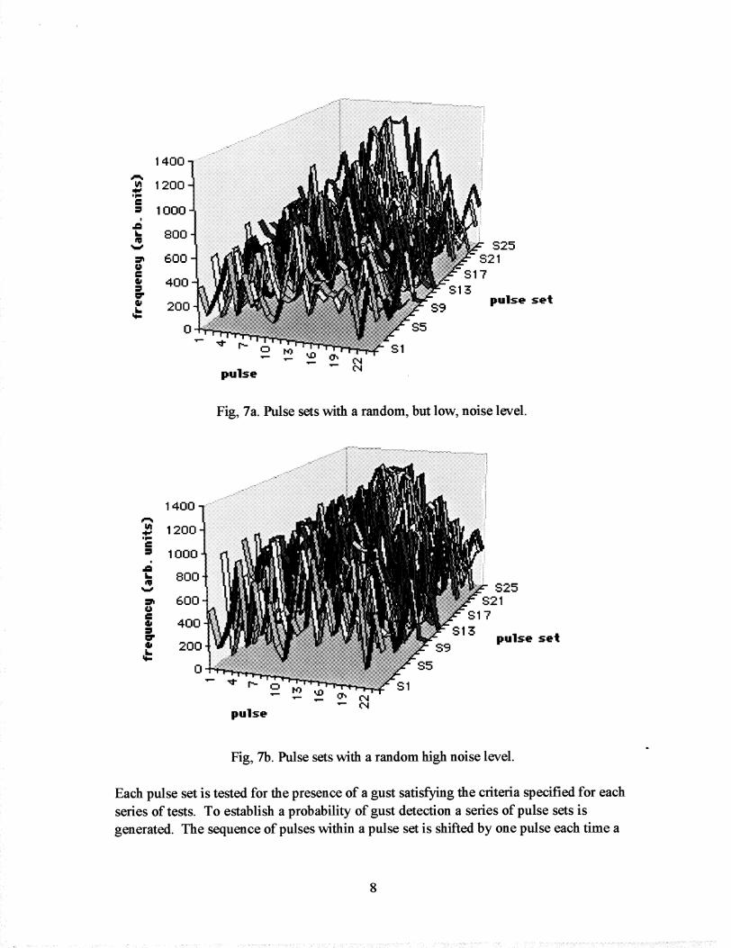
desired to produce gusts of any desired profile. Figures 7a and 7b display the estimator

output for two series of pulse sets, each with different random noise between sets, but

with the overall noise level higher in Fig. 7b.

A

Ak.

g_QC

gr

1400

1200

I000

800

600

400

200

0

pulse

S9

$5

2

$25$21

S17S13

pulse set

Fig, 7a. Pulse sets with a random, but low, noise level.

I//

Ill

g_

1400

1200

1000

800 iS25

600 $21= S1 7

400= S13=r pulse set• 200 S9

pulse

$1

Fig, 7b. Pulse sets with a random high noise level.

Each pulse set is tested for the presence of a gust satisfying the criteria specified for each

series of tests. To establish a probability of gust detection a series of pulse sets is

generated. The sequence of pulses within a pulse set is shifted by one pulse each time a

new set is begun such that each series consists of 25 identical pulse sets, except for the

permuted order and the noise component. For each set the detection of a gust is assigned

a value of 1.0 and non-detection a value of 0.0. These 25 values are averaged over the 25

pulse sets within the series to give a probability of gust detection.

As we examine the sensitivity of gust-detection probability to various gust characteristics

or other external parameters, an entire series of the type described above must be

generated for each set of characteristics. In Fig. 8 the upper surface represents gust-

detection probability, in this case as a function of both gust amplitude and overall noise

level. Each value was obtained through the generation of a series of pulse sets, with the

gust and noise amplitudes held constant within each series. A gust was def'med as a

change in estimated signal of at least 750 (code units) occurring over a pulse separation of

more than 2 pulses and less than 20 pulses.

1

Fig. 8. Gust-detection probability (upper surface and right-hand color legend) and

precursor quality (lower surface and left-hand color legend), both functions of gust

amplitude and overall noise level.

Precursors

As Fig. 2 suggests, the detection of precursors can increase the time available to respond

to gusts. Figure 8 illustrates this concept by allowing us to correlate by eye a measure of

the presence of a precursor with gust-detection probability. The measure we have used,

and referred to as precursor quality, is an overlap integral q

I f(t)g(t)dtq-

f (t) f (t)dt" (3)

where g(t) represents the leading edge of the "known" gust profile and f(t) is the

estimated signal. In the results presented here g(t) is simply the profile of the input to

the signal generator. In practice g(t) would be an EOF or closely related function. Before

the integral q is evaluated, f(t) and g(t) must be temporally aligned. This is currently

accomplished by means of a least-squares fit.

In examining Fig. 8 we see that, for low noise, gust-detection probability seems to

increase slightly (and unevenly) with respect to gust amplitude and seems to be very

roughly correlated with the precursor quality. For high noise, as we might expect, no

such general descriptions, however rough, seem to apply. Incorporating percursor quality

into our detection scheme is simply a matter of applying an additional test to the

frequency estimates. Presumably, after a period of calibration, the other tests could be

dropped, and we would be with a detection scheme capable of operating with fewer

pulses.

Sensitivity to Gust Parameters

Setting precursors aside for now, we examine the performance of our "raw" gust detection

scheme. The data presented in Fig. 9 is the result of testing to determine whether stronger

gusts are more easily detected than weaker gusts. At the same time different levels of

receiver noise are introduced. The noise-level scale is linear, with relative values ranging

from one to ten for all of the data in this section. The signal in all cases has a relative

amplitude (at the receiver) of three, such that the signal-to-noise ratio ranges from 3"1 to

3"10.

Initially, (no-averaging case) no sensitivity to gust amplitude is exhibited over this

parameter range. (We believe the rapid oscillations with respect to gust amplitude to be

an artifact of our method of pulse-set preparation, and that these oscillations could be

eliminated with further refinement.) If we apply gust detection to temporally averaged

frequency estimates of the same input signal, sensitivity to gust amplitude begins to

emerge. The averaging has the effect of reducing sensitivity overall, such that only the

stronger gusts are detected for this set of parameters. Adjusting the pass band of the

analog front end of the receiver so as to maintain the maximum possible dynamic range at

all times would be alternative method of adjusting the sensitivity. With regard to noise

level, very little sensitivity is exhibited over the range of values used in this study.

10

no averaging

three-point averaging

nine-point averaging

Fig. 9. Gust-detection probability vs. gust amplitude and noise level. The gust amplitude

scale represents a series of pulse sets. In this case, pulse set 1 has a relative gust

amplitude of 11; pulse set 2 has a relative gust amplitude of 12, and so on up to pulse set

25 with a relative gust amplitude of 35. The different levels of averaging are applied to

the frequency estimate before any further processing occurs.

Figure 10 looks at detection sensitivity as a function of gust duration (temporal width).

Again, little sensitivity is apparent until averaging is applied. Then we see that shorter

ll

gusts are more easily detected. With respect to noise level, we see, if anything, a higher

probability of detection for higher noise levels, possibly corresponding to false alarms.

no averaging

three-point averaging

'_iiiiiiiiii!i!iiiiiiiiii_

nine-point averaging

Fig. 10. Gust-detection probability vs. gust width and noise level. The gust-width scale

represents a series of pulse sets in manner similar to the gust-amplitude scale of Fig. 9. In

this case the range is relatively narrow, with pulse set 1 corresponding to a gust width of

roughly three pulses and pulse set 25 corresponding to a gust width of roughly five

pulses.

12

Conclusions

Methods for further minimizing the risk of unstart by making use of previous lidar

observations were investigated. EOFs are likely to play an important role in these

methods, and a procedure for extracting EOFs from data has been implemented. The new

processing methods involving EOFs could range from extrapolation, as discussed above,

to more complicated statistical procedures for maintaining low unstart risk.

We have also applied our basic gust-detection scheme to simulated wind-field data and

obtained reasonable performance. The extension of this scheme to include precursors

(EOF-based or otherwise) is straightforward. Exactly the same procedures are followed

up to the point of evaluating a set of frequency estimates against the gust criteria. At this

point, precursor quality is simply added as an additional criterion.

Acknowledgments

Useful comments and assistance were obtained from, Alex Thomson, Dave Soreide, Steve

Harmon, Dave Bowdle, Rod Frehlich, Steve Johnson, Philip Kromis, Rod Bogue, Grettel

von Laven, and Z.T. Deng.

References

° IL Bogue, H. Bagley, D. Soreide, and D. Bowdle, "Coherent lidar solution for the

HSCT supersonic engine inlet unstart problem," SPIE Proceedings, 2464-13, 1995.

2. S. von Laven, "1995 ACLAIM Technical Report", Alabama A&M University, 1995.

3. C. Carlin, Boeing Aerospace Corporation, private communication, 1995.

° P. Moin and R.D. Moser, "Characteristic-eddy decomposition of turbulence in a

channel," Journal of FluidMechamcs, 200, pp. 471-509, 1989.

. N. Aubry, P. Holmes, J.L. Lumley, and E. Stone, "The dynamics of coherent

structures in the wall region of a turbulent boundary layer," Journal of Fluid

Mechanics, 192, pp. 115-173, 1988.

6. M. Lo_we, Probability Theory, D. Van Nostrand, Princeton, NJ, 1963.

. J.L. Lumley, "The structure of inhomogeneous turbulent flows," Atmospheric

Turbulence and Radio Wave Propagation, A.M. Yaglom and V.I. Tatarskii, Eds.

Nauka, Moscow, pp. 166-176, 1967.

8. H.A. Panofsky, and J.A. Dutton, Atmospheric Turbulence, Models and Methods for

Engineering Applications, Wiley, New York, 1984.

13