simulation of indoor radon and energy...
TRANSCRIPT

Mälardalen University Press DissertationsNo. 190
SIMULATION OF INDOOR RADON AND ENERGY RECOVERYVENTILATION SYSTEMS IN RESIDENTIAL BUILDINGS
Keramatollah Akbari
2015
School of Business, Society and Engineering
Mälardalen University Press DissertationsNo. 190
SIMULATION OF INDOOR RADON AND ENERGY RECOVERYVENTILATION SYSTEMS IN RESIDENTIAL BUILDINGS
Keramatollah Akbari
2015
School of Business, Society and Engineering

Mälardalen University Press DissertationsNo. 190
SIMULATION OF INDOOR RADON AND ENERGY RECOVERYVENTILATION SYSTEMS IN RESIDENTIAL BUILDINGS
Keramatollah Akbari
Akademisk avhandling
som för avläggande av teknologie doktorsexamen i energi- och miljöteknik vidAkademin för ekonomi, samhälle och teknik kommer att offentligen försvaras
fredagen den 18 december 2015, 10.00 i Pi, Mälardalens högskola, Västerås.
Fakultetsopponent: Associate Prof. Anestis Kalfas, Aristotle University of Thessaloniki
Akademin för ekonomi, samhälle och teknik
Copyright © Keramatollah Akbari, 2015 ISBN 978-91-7485-236-3ISSN 1651-4238Printed by Arkitektkopia, Västerås, Sweden
Mälardalen University Press DissertationsNo. 190
SIMULATION OF INDOOR RADON AND ENERGY RECOVERYVENTILATION SYSTEMS IN RESIDENTIAL BUILDINGS
Keramatollah Akbari
Akademisk avhandling
som för avläggande av teknologie doktorsexamen i energi- och miljöteknik vidAkademin för ekonomi, samhälle och teknik kommer att offentligen försvaras
fredagen den 18 december 2015, 10.00 i Pi, Mälardalens högskola, Västerås.
Fakultetsopponent: Associate Prof. Anestis Kalfas, Aristotle University of Thessaloniki
Akademin för ekonomi, samhälle och teknik
AbstractThis study aims to investigate the effects of ventilation rate, indoor air temperature, humidity and usinga heat recovery ventilation system on indoor radon concentration and distribution.
Methods employed include energy dynamic and computational fluid dynamics simulation,experimental measurement and analytical investigations. Experimental investigations primarily utilizea continuous radon meter and a detached house equipped with a recovery heat exchanger unit.
The results of the dynamic simulation show that the heat recovery unit is cost-effective for the coldSwedish climate and an energy saving of about 30 kWh per floor area per year is possible, while it canbe also used to lower radon level.
The numerical results showed that ventilation rate and ventilation location have significant impactson both radon content and distribution, whereas indoor air temperature only has a small effect onradon level and distribution and humidity has no impact on radon level but has a small impact on itsdistribution.
ISBN 978-91-7485-236-3ISSN 1651-4238

In the world, there is only one excellence and one sin, the knowledge and the ignorance.
(J.M. Rumi, 1207–1273)


Acknowledgments
This thesis has been carried out at the Future Energy Center at Mälardalen University..I wish to express my gratitude to my previous main supervisor, Prof. Jafar Mahmoudi and my current main supervisor, Associate Prof. Kon-stantinos Kyprianidis for their continued encouragement and valuable sug-gestions during this work, for offering the possibility to do my PhD. studies in this field and for their support. I am also grateful to my co-supervisor Dr Robert Öman who supported me with many informative discussions. I would also like to include my gratitude for friendly cooperation to Prof. Erik Dahlquist, Bengt Arnryd and Adel Karim. Also, I am grateful to Dr David Ribé for the English language corrections, Mikael Gustafsson and Dr Jan Pourian and Dr Hamid Nabati for their valuable advice and assistance.
I would like to thank the Academic Center for Education, Culture and Re-search (ACECR) and the Technology Development Institute (TDI) for finan-cial support of this thesis. Furthermore, I am deeply indebted to cooperation from the environment section of Västerås Municipality, JBS, AB Company and EQUA AB for the use of IDA ICE, the Indoor Air Climate and Energy software program. I would also like to show my appreciation towards Hamid Afshar for providing supports and helping to test radon and obtain measure-ment data in his house for an extended period.
Finally, I want to thank my family – the encouragement and support from my beloved wife and our always positive and joyful sons is a powerful source of inspiration and energy. I would like to dedicate a special thought to my parents for their never-ending support.

Abstract
This study aims to investigate the effect on indoor radon concentration and distribution of ventilation rate, indoor air temperature, and humidity when using a heat recovery ventilation system.
Methods employed include energy dynamic simulations and computa-tional fluid dynamics, experimental measurements and analytical investiga-tions. Experimental investigations primarily utilize a continuous radon meter and a detached house equipped with a recovery heat exchanger unit.
The results of the dynamic simulation show that the heat recovery unit is cost-effective for the cold Swedish climate and an energy saving of about 30 kWh per 𝑚𝑚2 floor area per year is possible, while it can be also used to low-er radon level.
The numerical results showed that ventilation rate and ventilation location have significant impacts on both radon content and distribution, whereas indoor air temperature only has a small effect on radon level and distribution and humidity has no impact on radon level but has a small impact on its dis-tribution.

Summary
The main purpose of this doctoral dissertation is to investigate how the radon level and its distribution in indoor air are influenced by both the ventilation and by different conditions indoors. A heat recovery ventilation system could be a good choice from energy saving and indoor radon mitigation standpoints. The study uses two approaches in parallel. In the first approach, dynamic simulation is used to demonstrate the energy recovery potential. In the second approach, a detailed numerical model is developed and utilised to predict the indoor radon level and distribution with varying levels of ventila-tion rate, indoor air temperature and humidity.
The effect of a heat recovery ventilation system on both energy saving and radon mitigation was investigated in a detached house using IDA, ICE, Indoor Air Climate and Energy software program, analytical investigations and measurements. Then a finite volume method was applied using the com-putational fluid dynamics (CFD) ANSYS FLUENT software.
Although many research studies have been conducted on the effects of ra-don in soil and its properties on indoor radon, information about the influ-ence of indoor air conditions on indoor radon behaviour is rather scarce and merits further investigation. Furthermore, traditional methods of measuring indoor radon can only provide rough average values for the whole of a build-ing or a room for an entire year. This is unsafe and unacceptable from the indoor air quality viewpoint. Health organizations also emphasise that any level of radioactive elements such as radon may be carcinogenic.
Through the CFD simulations carried out in this study, the indoor radon level and distribution is predicted throughout a room and particularly in dead zones with insufficient ventilation rate. The simulations provide a good pic-ture of indoor radon distribution and help investigate the effect of different independent variables on indoor radon.
In this study, indoor radon activity concentrations were measured during the cold season for different ventilation rates using a new radon electronic meter (commercially known as R2) which can measure radon, temperature and relative humidity simultaneously. The measurements complement the theoretical analysis performed on the association between indoor radon level and ventilation rate, the height above the floor and economic analysis of installing a heat recovery unit considering life cycle costs.
The results of the dynamic simulation and theoretical analysis confirmed that the heat recovery unit is cost-effective for cold climates like Sweden and an energy saving of about 3,000 kWh per year or about 30 kWh per m2 floor area per year is possible.

The numerical simulation results show that ventilation rate and ventilation location have significant impacts on both radon content and radon distribu-tion, whereas indoor air temperature has a small effect on radon level and distribution, and humidity has no impact on radon level but has a small im-pact on its distribution. There was good agreement between analytical, measurement and simulation results concerning the association between indoor radon level, the height above the floor and ventilation rate.
It should be emphasised that this work represents the first step in the field with regard to using CFD to study the sensitivity of indoor radon level and its distribution in small residential buildings. The research is supported by a number of publications as well as unpublished results which are shown for the first time in the main body of this thesis. It is hoped that the present study will serve as a stepping stone for further work in the field by the other re-searchers.

Sammanfattning
Huvudsyftet med denna doktorsavhandling är att undersöka hur radonhalt och dess fördelning i inneluft påverkas av både ventilation och av olika för-hållanden inomhus. Ett fläktstyrt ventilationssystem med en värmeväxlare mellan från- och tilluft kan bidra till både mindre värmeförluster och lägre radonhalt i inneluften. I denna studie används två metoder parallellt. Den första metoden är dynamisk simulering av energibalans med fokus på vär-meväxling. Den andra metoden avser en detaljerad numerisk modell som utvecklats och tillämpats för att förutsäga hur radonhalt och fördelning av radonhalt i inneluft påverkas av uteluftsflöde och inneluftens temperatur och luftfuktighet.
Ett fristående småhus med en värmeväxlare mellan från- och tilluft stude-rades avseende både energihushållning och radonbegränsning med datapro-grammet IDA ICE (Indoor Climate and Energy), med analytiska undersök-ningar och med mätningar. För en detaljerad numerisk modell användes sedan en finit volymmetod med CFD (Computational Fluid Dynamics) i dataprogrammet ANSYS FLUENT.
Många studier har gjorts om markradon och dess allmänna påverkan på radonhalten i inneluft. Det finns dock mycket begränsat med information om hur olika förhållanden inomhus kan påverka radon i inneluft och detta moti-verar vidare undersökning. Dessutom brukar traditionella mätmetoder för radon bara ge medelvärden för ett visst rum eller en viss byggnad ofta upp-skattat för ett helt år. Detta kan sägas vara osäkert och oacceptabelt med hänsyn till den stora betydelsen av inneluftens kvalitet. Hälsoorganisationer betonar också att all joniserande strålning från till exempel radon kan vara cancerframkallande.
Simuleringar med CFD användes i denna studie för att förutsäga radon-halten och dess fördelning i rum som även innehåller stagnationszoner med mycket dålig ventilation. Simuleringarna kan ge en bra uppfattning om ra-donhaltens fördelning och kan även visa hur olika variabler inverkar på ra-donhalten.
Samtidiga mätningar av radonhalt, lufttemperatur och relativ luftfuktighet gjordes med olika uteluftsflöde vintertid med en ny elektronisk radonmätare som kommersiellt är känd som R2. Mätningarna kompletterar den teoretiska analysen avseende sambandet mellan radonhalt å ena sidan och uteluftsflöde och höjd över golvet å andra sidan, och även när det gäller en ekonomisk analys med livscykelkostnader avseende värmeväxling.
Resultat från den dynamiska simuleringen och den teoretiska analysen bekräftar att värmeväxlaren i detta fall är kostnadseffektiv för kalla klimat

såsom i Sverige med en möjlig energibesparing om ca 3 000 kWh per år eller ca 30 kWh per m2 golvarea och år.
Resultat från de numeriska simuleringarna visar att uteluftsflöde och ven-tilationsdonens placering har betydande inverkan på både radonhalten och dess fördelning, medan innetemperaturen har en liten inverkan på radonhal-ten och dess fördelning. Vidare framgår att luftfuktigheten inte inverkar på genomsnittlig radonhalt, men har en liten inverkan på radonhaltens fördel-ning. Överensstämmelsen var god mellan resultaten från analys, mätningar och simuleringar avseende sambandet mellan radonhalt å ena sidan och uteluftsflöde och höjd över golvet å andra sidan.
Det bör framhållas att det här arbetet utgör ett första steg inom området avseende CFD-simulering för detaljerade studier av radonhalt och dess för-delning i småhus. Forskningen stöds av ett antal publikationer samt opubli-cerade resultat som visas för första gången i huvuddelen av denna avhand-ling. En förhoppning är att denna studie kommer att fungera som en språng-bräda för fortsatt arbete inom området av andra forskare.
List of Papers included
This thesis is based on the following papers, which are referred to in the text by their Roman numerals.
I. Akbari, K. & Öman, R. (2013). Impacts of heat recovery ventilators on
energy savings and indoor radon level. Management of Environmental Quality Journal, Vol. 24, No. 5, pp. 682–694.
II. Akbari, K., Mahmoudi, J. & Ghanbari, M. (2013). Simulation of Venti-lation Effects on Indoor Radon. Management of Environmental Quality Journal, Vol. 24, No. 3, pp. 394–407.
III. Akbari, K. & Mahmoudi, J. (2012). Effects of Heat Recovery Ventila-tion Systems on Indoor Radon. Proceedings of ECOS 2012 - the 25th in-ternational conference on Efficiency, Cost, Optimization, Simulation and Environmental Impact of Energy Systems, June 26-29, 2012, Perugia, Italy ECOS 2012. Available at: http://www.ecos2012.unipg.it/public/ proceedings/pdf/buces/buces_ecos2012_329.pdf.
IV. Akbari, K. & Mahmoudi, J. (2013). Influence of Indoor Air Conditions on Radon Concentration in a Detached House. Journal of Environmental Radioactivity, No. 116, pp. 166–173.
Reprints were made with permission from the respective publishers.
List of Publications not included
In completion of this thesis and the papers listed above, ideas, data meas-urements, computations, modeling and simulations, and analyses were car-ried out by the author. I have been assisted by my main supervisor, co-supervisor, reviewers and co-authors in adding further improvements to the work. Papers and other publications excluded from this thesis are as follows.
Licentiate thesis I. Akbari, K. (2009). Impact of Radon Ventilation on Indoor Air Quali-
ty and Building Energy Saving. Mälardalen University Press. ISBN 978-91-86135-39-3. Available at http://mdh.diva-portal.org/smash/get/diva2:237857/FULLTEXT01.pdf
Papers II. Akbari, K. & Mahmoudi, J. (2008). Simulation of Radon Mitigation
and Ventilation in Residential Building. Printed in the 49th Scandi-navian conference on Simulation and Modeling (SIMS 2008). ISBN-13-978-82-579-4632-6.
III. Akbari, K., Mahmoudi, J. & Öman, R. Ventilation Strategies and Radon Mitigation in Residential Buildings. Submitted to Indoor Air International Journal of Indoor Environment and Health. ID: INA-09-09-156.
IV. Akbari, K. & Mahmoudi, J. (2009). Influence of Residential Ventila-tion on Radon Mitigation with Energy Saving Emphasis. Scientific Conference on "Energy system with IT" March 2009, Stockholm. ISBN 978-91-977493-4-3.

Table of Contents
1 INTRODUCTION ..................................................................................... 1 Background ...................................................................................... 1 Problem description and motivation ................................................. 3 Aims and objectives ......................................................................... 4 Methods, limitations and research process ....................................... 4 Thesis outline ................................................................................... 5 Summary of included papers ............................................................ 6 Contribution to knowledge ............................................................... 8
2 LITERATURE REVIEW ............................................................................ 9 Indoor radon levels, energy use and heat recovery ventilation
system ............................................................................................... 9 Ventilation effect and Indoor Radon Mitigation ............................. 12 Radon transport mechanisms and environmental conditions effects
........................................................................................................ 12 2.3.1 Radon concentration equation in a ventilated room ................... 14 2.3.2 The effects of temperature and humidity on the pressure field .. 14
Radon modeling methods ............................................................... 15 3 MATERIALS AND METHODOLOGY ...................................................... 17
Materials ......................................................................................... 17 3.1.1 Case study house ........................................................................ 17 3.1.2 Heat recovery unit ...................................................................... 18 3.1.3 Radon detectors .......................................................................... 20
Research methods ........................................................................... 21 3.2.1 Measurement .............................................................................. 21 3.2.2 Analytical analysis ..................................................................... 22 3.2.3 Economic analysis ...................................................................... 23 3.2.4 Heating degree days (HDD) calculations ................................... 23 3.2.5 Ventilation loss ........................................................................... 24 3.2.6 The life cycle cost analysis of heat recovery ventilation system 25
Energy dynamic simulation ............................................................ 26 Computational fluid dynamics (CFD) ............................................ 27
4 NUMERICAL MODELING PROCEDURE ................................................. 29 Discretization methods ................................................................... 29
4.1.1 Finite control volume analysis ................................................... 30

Governing equations used .............................................................. 30 Turbulence model ........................................................................... 34 Boundary conditions and input data ............................................... 35
4.4.1 Inlet Vent .................................................................................... 35 4.4.2 Outlet .......................................................................................... 37 4.4.3 Outer Surfaces ............................................................................ 37 4.4.4 Internal Surfaces ......................................................................... 38 4.4.5 Floor Zone .................................................................................. 38
The House Plan Geometry .............................................................. 39 Parameters Variation Range ........................................................... 40 Materials Properties ........................................................................ 41 Relative Humidity .......................................................................... 42 Defined Functions .......................................................................... 45
Convergence Criteria ...................................................................... 45 Near-wall treatment ........................................................................ 46 Mesh Independence Study .............................................................. 50 Examination of convergence criteria .............................................. 54
5 RESULTS AND DISCUSSION .................................................................. 63 Radon measurement ....................................................................... 63 Analytical analysis of radon level in the case study house ............. 68 Dynamic energy simulation and calculation .................................. 68
5.3.1 Economic analysis of the heat recovery ventilation unit ............ 69 Results and discussion of numerical modelling ............................. 71
5.4.1 Air Change Rate Effects on Indoor Radon Content ................... 71 5.4.2 Temperature Changes Effects on Indoor Radon Concentration . 76 5.4.3 Effects of Relative Humidity Changes on Indoor Radon
Concentration ............................................................................. 79 Model validation and result comparison ........................................ 81
6 CONCLUSIONS AND FUTURE WORK ..................................................... 83 Dynamic simulation and heat recovery analysis ............................ 83 Numerical Simulation ..................................................................... 84 Future work .................................................................................... 85
REFERENCES ................................................................................................... 87 APPENDICES .................................................................................................... 91 APPENDIX A: IDA, BOUNDARY CONDITIONS AND INPUT DATA ................ 93 APPENDIX B: RADON TRANSPORT EQUATIONS AND INDOOR CONDITIONS
97 PAPERS .............................................................................................................. 1
List of Figures
Figure 1. Ground floor plan and zone divisions of the case study house.... 18 Figure 2. Air flows through the rotary heat exchanger ............................... 19 Figure 3. The rotary heat exchanger installed in the building .................... 20 Figure 4. The R2 continuous radon meter .................................................. 21 Figure 5. The house plan geometry............................................................. 39 Figure 6. Room1 geometry ......................................................................... 40 Figure 7. A sample of the meshed model ................................................... 50 Figure 8. Average radon concentration for different mesh sizes ................ 52 Figure 9. Average static temperature for different mesh sizes ................... 52 Figure 10. Radon flow rate in the outlet for different mesh sizes ................. 53 Figure 11. Radon concentration profile along a vertical line in the middle of
the room for different mesh sizes ................................................ 53 Figure 12. Average radon concentration versus iterations for the case N11 54 Figure 13. Average indoor static temperature versus iterations for the case
indicated with N11 ...................................................................... 55 Figure 14. Radon flow rate in the outlet versus iterations for the case indicated
with N11 ...................................................................................... 56 Figure 15. Residuals versus iterations for the case indicated with N11 ....... 57 Figure 16. Radon level measurements versus ventilation rate ...................... 65 Figure 17. Radon level (green curve) and temperature (purple curve). ........ 66 Figure 18. Radon level changes versus measurement height above the room
floor ............................................................................................. 66 Figure 19. Average radon levels versus height (0-200 cm from the floor) ... 67 Figure 20. Average radon levels versus height (0-50 cm from the floor) ..... 67 Figure 21. Average radon content for different air change rates at T = 21°C
and RH = 40% ............................................................................. 72 Figure 22. Radon concentration along a vertical line in the middle of the room
for N3 (Ach = 0.5hr, T = 21°C, RH = 40%) ................................ 72 Figure 23. Radon content along a vertical line in the middle of the room for
N12 (Ach = 0.25 hr-1, T = 21 °C, RH = 40%) ............................. 73 Figure 24. Position of two vertical planes in the middle of room for showing
distribution of different quantities within the room..................... 73 Figure 25. Contours of radon concentration (Bqm-3) in two vertical planes in
the middle of room for N3 (Ach=0.5 hr-1, T=21 °C, RH=40%) .. 74 Figure 26. Contours of air velocity (ms-1) in two vertical planes in the middle
of room for N3 (Ach = 0.5 hr-1, T = 21 °C, RH = 40%) .............. 74

Figure 27. Contours of radon concentration (Bqm-3) in two vertical planes in the middle of room for N12 (Ach = 0.25 hr-1, T = 21 °C, RH = 40%)................................................................................... 75
Figure 28. Contours of air velocity (ms-1) in two vertical planes in the middle of room for N12 (Ach = 0.25 hr-1, T = 21 °C, RH = 40%) .......... 75
Figure 29. Average radon concentration in the room for different temperatures at Ach = 0.5 hr-1 and RH = 40% .................................................. 76
Figure 30. Radon concentration along a vertical line in the middle of room for different temperatures (15 to 23°C) at Ach = 0.5 hr-1 and RH = 40% ..................................................................................................... 77
Figure 31. Contours of radon concentration (Bqm-3) in two vertical planes in the middle of room for N3 (Ach = 0.5 hr-1, T = 21 °C, RH = 40%) ..................................................................................................... 78
Figure 32. Contours of radon concentration (Bqm-3) in two vertical planes in the middle of room for N4 (Ach = 0.5 hr-1, T = 23 °C, RH = 40%) ..................................................................................................... 78
Figure 33. Contours of radon concentration (Bqm-3) in two vertical planes in the middle of room for N4 (Ach = 0.5 hr-1, T = 21 °C, RH = 40%) ..................................................................................................... 80
Figure 34. Contours of radon concentration (Bqm-3) in two vertical planes in the middle of room for N7 (Ach = 0.5 hr-1, T = 21 °C, RH = 50%) ..................................................................................................... 80

List of Tables
Table 1. Physico-chemical characteristics of radon (Keith S, 2012) ........... 2 Table 2. Features of the different numerical simulations in the publications7 Table 3. Annual radon average concentration in Västerås, Sweden .......... 10 Table 4. Radon levels and remediation techniques (Radiological Protection
Institute of Ireland, 2010) ............................................................ 12 Table 5. The operation ratings of the unit ................................................. 20 Table 6. Date and time period of the measurements ................................. 22 Table 7. Velocity and turbulence intensity for different ventilation rates . 37 Table 8. Sizes of the building elements ..................................................... 40 Table 9. Different cases studied in this work ............................................ 41 Table 10. Properties of the fluids (Lide, 2004) ............................................ 42 Table 11. Properties of the solids (Lide, 2004) ........................................... 42 Table 12. Mass fraction of water vapor for different relative humidity and
temperatures ................................................................................ 45 Table 13. Average radon concentration, average static temperature and radon
flow rate in the outlet for different mesh sizes ............................ 51 Table 14. The heat rejection to outdoor environment through each outer
surface, case N11 ......................................................................... 60 Table 15. Measured indoor radon levels (Bqm-3) ........................................ 64 Table 16. Radon level versus ventilation rate by measurement and analytic
methods ....................................................................................... 68 Table 17. Dynamic simulation and energy calculation results .................... 69 Table 18. Values used for life cycle cost analysis ....................................... 70 Table 19. Ventilation system life cycle cost analysis .................................. 70 Table 20. Average radon content for different air change rates at T = 21 °C
and RH = 40% ............................................................................. 71 Table 21. Average radon concentration in the room for different temperatures
at Ach=0.5 hr-1 and RH=40% ...................................................... 76 Table 22. Average radon concentration for different relative humidity at Ach
= 0.5 hr-1 and T = 21 °C ............................................................... 79 Table 23. Indoor radon levels obtained by different methods ..................... 81 Table 24. Indoor radon for different heights above the floor ...................... 82 Table 25. The impacts of parameters on indoor radon level and distribution84

Nomenclature and abbreviations
Symbols
𝑨𝑨 Surface (m2) 𝑨𝑨𝑨𝑨 Radium activity (Bq kg-1) 𝑪𝑪 Radon activity concentration (Bq m-3) Cf Skin friction Cp Specific heat capacity (J kg-1 K-1) D Effective diffusion coefficient (m2s−1) Dh Hydraulic diameter (m) 𝑬𝑬 Radon exhalation rate(Bq𝑚𝑚−2ℎ−1) f Radon emanation coefficient 𝑮𝑮 Radon generation rate (Bq m-3 s-1) hc Heat transfer coefficient (W m-2 K-1) 𝒊𝒊 Interest rate (%) I Turbulence intensity
𝑰𝑰𝒒𝒒 Net present value factor 𝒌𝒌 Thermal conductivity (W m-1 K-1) K Turbulent kinetic energy (m2 s-2)
Mw Molecular weight m Mass flow rate (kg s-1) n Time in year unit P Pressure (Pa) q Annual energy cost escalation rate (%) R Specific gas constant (J mol-1 K-1) T Temperature (K) 𝑽𝑽 Volume (m3) V Flow velocity vector (m s-1)
u, v, w Velocity components in x, y, and z coordinates (m s-1) 𝜼𝜼𝒕𝒕 Temperature efficiency 𝜼𝜼𝒘𝒘 Moisture efficiency 𝝀𝝀𝒗𝒗 Air change rate(h−1) 𝝆𝝆 Density (kg m-3)
𝝀𝝀𝑹𝑹𝑹𝑹 Radon decay constant (s-1 or h-1) 𝛆𝛆 Turbulent dissipation rate (m2 s-3) µ Molecular viscosity (kg s-1 m-1) 𝝁𝝁𝒕𝒕 Turbulent viscosity (kg s-1 m-1) ν Kinematic viscosity (m2 s-1) 𝜺𝜺 Porosity
𝝉𝝉𝒘𝒘 Wall shear stress

Abbreviations
Ach Air change rate ASHRAE American society of heating, refrigerating and
air conditioning engineering ATD Alpha track detector CFD Computational fluid dynamics CHTC Convective heat transfer coefficient CRM Continuous radon monitor DHW Domestic hot water HVAC Heating, ventilation and air conditioning HRV Heat recovery ventilation HDD Heat degree days IAQ Indoor air quality kWh Kilowatt-hour MF Mass fraction
PDE Partial differential equations Re Reynolds number RH Relative humidity Rn Radon-222 SST Shear stress transport TWh Terawatt-hour


1
1 Introduction
Background
People in developed countries regularly spend more than 90 % of their time in confined and enclosed spaces, i.e. in homes, offices and vehicles. More than two thirds of this time is spent in residential buildings. Buildings act as a shelter and protect people from heat, cold, sunshine, noise, pollutants and other inconveniences. However, these shelters are not as safe as they could be, because they contain many indoor pollutants. Pollutants create indoor air quality (IAQ) problems which affect human health, productivity and com-fort. Unfortunately the variety and amount of pollutants are continuously increasing (Zhang Y. , 2004; WHO, 2009).
Radon is one of the major and most harmful indoor pollutants in many countries, such as the Scandinavian countries, the U.S., U.K., etc. Radon is estimated to account for more than 3,000 and 21,000 deaths annually from lung cancer in the UK and US respectively (Nilsson, 2006; EPA, 2008).
Sweden is one of the countries with the highest indoor radon concentra-tions in the world. This radon originates from uranium-rich soils and rocks such as alum-shale and uranium-rich granites (Sundal, Henriksen, Lauritzen, & Soldal, 2004).
Radon in the environment is present as a radioactive ground gas which exists in soil, water, air and in some natural gas. This radioactive gas mixes with air and is quickly diluted in the atmosphere. However, radon which enters enclosed spaces can accumulate and reach relatively high levels in some places, especially in buildings with insufficient ventilation (Malanca, Cassoni, Dallara, & Pessina, 1992).
General methods to control the levels of indoor pollutants are by source control, e.g. removal, replacement by alternative materials, sealing or dilu-tion, or by removal by ventilation and air cleaning. When the radon regulato-ry limit is set in the range of 600 Bq/m3 or less, ventilation becomes a cost-effective and applicable method to dilute radon contamination and maintain IAQ in existing under-ventilated buildings (Radiological Protection Institute of Ireland, 2010), i.e. buildings with ventilation below the typical air ex-change requirement of 0.5 hr-1. Ventilation blows fresh outdoor air into the room and reduces pollutant concentrations by mixing and dilution. However, building ventilation in turn leads to increased energy consumption in the
2
building sector. An optimal ventilation rate is therefore important for both people and governing authorities (in the case of housing associations).
Radon-222 (simply referred to as "radon") is a radioactive and inert gas which decays into alpha particles with a half-life of 3.82 days. This radioac-tive gas is colorless, odorless, tasteless, and is therefore undetectable without the use of specific instruments. It originates from decay chains of uranium and radium and is naturally occurring around the world. Radon in its gaseous form (at normal temperatures) is present throughout the earth's crust at dif-ferent concentrations which vary as a function of the nature of the soil. Some regions may therefore have serious issues with radon, as is the case in Swe-den, while others may have very limited or no concerns at all.
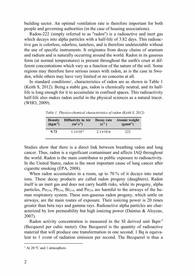
In standard conditions1, characteristics of radon are as shown in Table 1 (Keith S, 2012). Being a stable gas, radon is chemically neutral, and its half-life is long enough for it to accumulate in confined spaces. This radioactivity half-life also makes radon useful in the physical sciences as a natural tracer. (WHO, 2009).
Table 1. Physico-chemical characteristics of radon (Keith S, 2012)
Density (kgm-3)
Diffusivity in Air (m2 s-1)
Decay rate (s-1 )
Atomic weight (gmol-1)
9.73 1.1×10⁻⁵ 2.1×10⁻⁶ 222
Studies show that there is a direct link between breathing radon and lung cancer. Thus, radon is a significant contaminant and affects IAQ throughout the world. Radon is the main contributor to public exposure to radioactivity. In the United States, radon is the most important cause of lung cancer after cigarette smoking (EPA, 2008).
When radon accumulates in a room, up to 70 % of it decays into metal ions. These decay products are called radon progeny (daughters). Radon itself is an inert gas and does not carry health risks, while its progeny, alpha particles, Po214, Pb214, Bi214, and Po218 are harmful to the airways of the hu-man respiratory system. These non-gaseous radon progeny, which settle on airways, are the main routes of exposure. Their ionizing power is 20 times greater than beta rays and gamma rays. Radioactive alpha particles are char-acterized by low permeability but high ionizing power (Dainius & Aloyzas, 2007).
Radon activity concentration is measured in the SI derived unit Bqm-3 (Becquerel per cubic meter). One Becquerel is the quantity of radioactive material that will produce one transformation in one second; 1 Bq is equiva-lent to 1 event of radiation emission per second. The Becquerel is thus a 1 At 20 ºC and 1 atmosphere.

3
measure of the activity rate (and not the energy) of radiation emission from a source.
The building sector accounts for almost 40 % of the world’s energy use, and exceeds the transportation sector in terms of carbon emissions (Zhang & Cooke, 2010). Most of the energy use in the sector is related to heating, ven-tilation and air conditioning, which together account for 55 % of the energy use in residential buildings (Zhang & Cooke, 2010). In Sweden for example, about 61 % of energy used in the building sector is used for space heating and domestic hot water (Swedish Energy Agancy, 2010). It is important from the energy conservation point of view that ventilation rates are not ex-cessive, but at the same time they should be sufficient to ensure good IAQ. Radon reduction strategies should also aim to consider problems related to radon sources and transport processes to be efficient and cost-effective. Strategies can include active and passive soil depressurization, barriers and membranes, sealing entry routes, sealing building material surfaces and ven-tilation of occupied spaces.
Sometimes a combination of all these strategies may be necessary, partic-ularly in buildings with highly elevated radon levels. This thesis focuses on ventilation strategy by using a heat recovery ventilation system and de-scribes how to simultaneously improve the complications related to energy use and indoor radon concentration.
Problem description and motivation
Global energy consumption, particularly in the building sector is growing, and the use of energy-efficient technologies in ventilation systems has an important role to play in energy savings and emissions reduction.
Reducing radon in residential buildings is a significant problem from the viewpoints of IAQ, adverse health effects and energy savings. Reducing radon by means of forced ventilation inevitably leads to higher energy use. Heat recovery ventilation (HRV) systems as an energy-efficient technology can recover energy in exhaust air that would otherwise escape, both reducing energy use and balancing indoor and outdoor pressure to reduce radon con-centration.
Earlier studies (Fournier, Groetz, & Jacob, 2005; Narula, Saini, Goyal, & Chauhan, 2009) in this field have focused on factors affecting radon distribu-tion in soil and its characteristics. Some very recent and concurrent studies (Chauhan, Joshi, & Agarwal, 2014; Kumar, Chauhan, & Sahoo, 2014), are focusing on the comparison of CFD simulation results of radon concentra-tion and exhalation rates with experimental measurements indicating the importance of research on the indoor radon problem.

4
However, these studies do not explain how physical and environmental factors affect indoor radon concentration. The present study considers differ-ent indoor temperature and humidity conditions, ventilation rates, and other possibly important parameters to determine their effects on indoor radon distribution and concentration.
HRV systems are a well-known technology in Europe and are used as en-ergy-efficient systems. A HRV system can provide the required indoor con-ditions in several ways. For instance, it can balance the pressure difference due to supply and exhaust with fans and thus control indoor radon level. This study intends to improve the research community’s understanding of the conditions and the extent to which HRV technology can be applicable and cost-effective for indoor radon control relative to other mitigation methods.
In this study I use computational fluid dynamics (CFD) and measurement techniques to show the influence of several parameters on indoor radon level in a detached house. CFD is used to simulate and estimate indoor radon con-centrations and dynamic simulation is employed to analyze energy use by means of a rotary heat exchanger installed in the house.
Aims and objectives
The main aim of this work is to investigate the influence of ventilation, in-door temperature and humidity on radon mitigation using measurement, dynamics and numerical simulation from the viewpoints of energy savings and indoor air radon quality.
The research questions are:
Is it possible to use CFD to simulate and predict indoor radon distribu-tion in residential buildings with and without HRV?
What is the indoor radon distribution suggested by the CFD results? Under what conditions is a HRV system economically appropriate for reducing indoor radon in residential buildings relative to other mitigation methods?
What is the relationship between indoor temperature, indoor humidity, position of the supply and exhaust air terminal devices, and indoor radon level and distribution?
Methods, limitations and research process
Methods:
In this study, dynamic and CFD simulation, measurement and analytical methods have been used.

5
Limitations:
In the work described in this thesis, several assumptions have been made for simplicity and to comply with computational limitations (a High Perfor-mance Computing facility was not available for this study). These limitations and assumptions have potential to be developed and modified in future stud-ies using other CFD methods and by considering more complicated build-ings or rooms. For instance, the effects of residents and their furnishings, as well as the effect of non-ideal airtightness (leakages) in the building have been ignored in this work. Another assumption used throughout the thesis is that ventilation is provided by mechanical means (and with heat recovery) as opposed to other ventilation solutions. Assumptions have also been made regarding constant radon generation rate and outdoor conditions, as well as simplifications in the numerical modeling and intrinsic limitations of CFD techniques because of discretization and semi-empirical turbulence modeling methods.
Research process:
1. Investigating and gathering data on radon in recent years in the case study house.
2. Collecting new measurements with a continuous radon monitor in dif-ferent situations and under different temperature and relative humidity conditions.
3. Evaluating a heat recovery ventilation system. 4. Dynamic simulation using IDA 4.1 software. 5. CFD simulation using the ANSYS FLUENT 14 package.
Thesis outline
This thesis is broadly organized on two levels. The first level considers the role of a heat recovery ventilation system in energy saving and indoor radon control using life cycle cost to show its cost-effectiveness (Paper I). The second level considers indoor radon and effects of indoor air conditions in-cluding temperature, humidity and ventilation rate (papers II–IV).
The thesis comprises of six chapters and the contents are outlined as fol-lows:
Chapter 1 Introduction: background, problem description, motivation, objectives, thesis scope and outline.
Chapter 2 Literature review: review of heat recovery ventilation system, radon mitigation, radon transport mechanisms and modeling.

6
Chapter 3 Materials and Methodology: case study house, radon detec-tors, dynamics and CFD simulation packages.
Chapter 4 Numerical modeling procedure: discretization of radon transport equation, indoor radon modeling, boundaries, geometry and ma-terials.
Chapter 5 Results and discussion: results and discussion of radon meas-urement, dynamic simulation, economic analysis and numerical model-ing.
Chapter 6 Conclusion and future works: dynamic simulation and heat recovery analysis, numerical simulation and future works.
Summary of included papers
Paper I: Paper I focuses on dynamic simulation and energy recovery calculations. The results confirm that using a heat recovery unit can meet energy saving and radon mitigation needs simultaneously. It is shown how a heat recovery ventilation system means that an increased outdoor air flow rate can be com-bined with a comparatively limited increase in the energy demand for space heating in order to dilute and lower indoor radon levels. Life cycle cost anal-ysis also indicates that a heat recovery ventilation system can be cost-effective.
Paper II: This paper presents the first simple 3-D model to simulate radon generated from soil using CFD and the FLUENT software package. This work investi-gates the effects of ventilation rate, exhaust fan and supply fan on indoor radon. The results show that the effects of supply air terminal device location on radon level and distribution are distinguishable under different supply air flow rates. Compared to an exhaust fan, a supply fan has a greater impact on radon mitigation. Air leakages through doors and windows can have a simi-lar effect on indoor radon behavior to a supply fan. Of course this by no means a general conclusion, but an example from specific calculations on a particular type of residential building.
Paper III: In this paper the effects of ventilation rates, temperature, humidity and pres-sure is investigated on indoor radon. Results of numerical studies indicated that changes of ventilation rate, indoor temperature and moisture by means of ventilation systems have significant effects on indoor radon content. Ven-tilation rate was inversely proportional to indoor radon concentration. Mini-

7
mum radon levels were estimated in the range of thermal comfort, i.e. at 21℃ and relative humidity between 50–70%.
The approach of this paper is similar to Paper II, but the case study house is modeled without soil section and using fine grids.
Paper IV: This study uses an improvement over the model described in paper III. A heat recovery ventilation system unit was used to control the ventilation rate. As well as ventilation rate, this model considers the effects of indoor air temperature and relative humidity. The results from analytical solution, measurements and numerical simulation showed that air change rate had a significant effect on indoor radon concentration but indoor air temperature and moisture had little effect.
Overview: This thesis used the K-ω turbulence model in ANSYS FLUENT 14.0 instead of the K-ε model in FLUENT 6.4 used in papers II–IV with the aim of im-proving the near wall treatment. The dynamic simulations and calculations on heat recovery presented in Paper I are the same as the results presented in the main body of this thesis. Table 2 presents an overview of the different numerical simulations present-ed in papers II–IV and in the main body of this thesis.
Table 2. Features of the different numerical simulations in the publications
Publication Geometry Model Kinds of air conditions
Turbulence and grid cells
Paper II House without partitions
Soil radon, Mixture of air and radon in species model
Exhaust and sup-ply fans separately
Turbulence k-ε model, 200,000 hexahedral cells
Paper III All rooms Indoor radon, Mixture of air, moisture and radon in species model
Temperature, Humidity, Pres-sure difference, Balanced ventila-tion
Turbulence k-ε model 370,000 hexahedral cells
Paper IV All rooms Indoor radon, Mixture of air, moisture and radon in species model
Temperature, Humidity, Bal-anced ventilation
Turbulence k-ε model 700,000 hexahedral cells
Thesis One room Indoor radon, Mixture of air, moisture and radon in species model
Temperature, Humidity, Ba-lanced ventilation
Turbulence k-ω model 2,700,000 hexahedral cells

8
Contribution to knowledge
The literature survey reveals that there is little or no research available in the public domain regarding the analysis of the effect of heat recovery ventila-tion on indoor radon mitigation using advanced CFD simulations. With this in mind, the author’s efforts have focused on the development of models and methods of numerical simulation of indoor radon, as well as on the meas-urement of indoor radon, temperature and relative humidity with advanced equipment.
The author’s contribution to the knowledge in the area can be summarized as follows:
Development of CFD models for analyzing indoor radon concen-tration and distribution in one-family residences.
Analysis of IAQ focusing on indoor radon using the aforemen-tioned models. The application of a HRV system was considered in detail because of its capacity for controlling indoor radon con-centration as well as indoor temperature, pressure, moisture and ventilation rate. Displacement ventilation was assessed as a likely candidate for ventilation with regard to radon mitigation; the sim-ulation results indicate that the performance of such a system is likely to be dependent on the vertical position of its installation within the occupied zone.
It is important to note that the presented work is supported by three peer-reviewed journal publications and one peer-reviewed conference paper.

9
2 Literature review
This chapter provides a review of the literature on previous relevant re-search: energy use and heat recovery ventilation system; ventilation and indoor radon mitigation; radon transport mechanisms and effects of environ-mental conditions; radon modeling methods.
Indoor radon levels, energy use and heat recov-ery ventilation system
The World Health Organization recommends 100 Bqm-3 as a new indoor radon action level (WHO, 2009). This value is currently 200 Bqm-3 in Swe-den. Based on a recent radon survey in Sweden, 35 % of all monitored small houses and 28 % of apartments had radon levels that exceeded 200 Bqm-3 (Hjelte, Ronquist, & Ronnqvist, 2010).
Sweden has the second highest indoor radon levels among Scandinavian countries. Based on the radon risk map of a municipality in Sweden, about 70 % of Swedish surface (ground) has normal risk, with radon content of 10,000–50,000 Bqm-3 due to bedrocks and soil with low normal Uranium content and average permeability (Dubois, 2005).
Around 300,000 buildings in Sweden include uranium-bearing building materials in the form of lightweight (blue) concrete which is used for inter-nal and external walls and sometimes in floor structures. The radon level in houses in which a substantial proportion of the building material consists of this type of concrete is elevated. Radon exhalation rate (E) from building materials in some Swedish buildings built between 1929 and 1975 is in the range 0.01 to 0.07 Bqm−2s−1 (Clavensjö & Åkerblom, 1994).
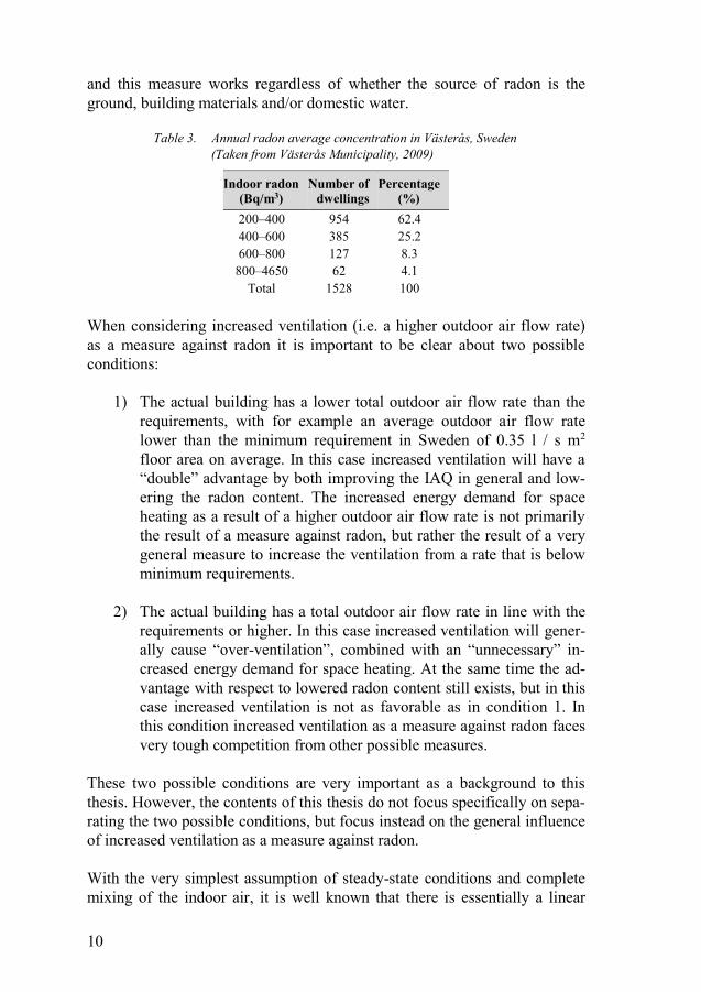
In a survey of radon measurement in 1,528 dwellings by Västerås munic-ipality produced with such material (Table 3), almost all homes were con-taminated with radon levels higher 200 Bqm-3, and more than 87 % had radon levels in the range of 200–600 Bqm-3, in which the radon level can be lowered using a heat recovery ventilation system. The minimum, maximum and average indoor radon levels found in this survey were 201; 4,650 and 405 Bq/m3 respectively.
These dwellings need mitigation measures in to lower the radon content at least to 100 Bqm-3. Increased ventilation is one possible general measure,
10
and this measure works regardless of whether the source of radon is the ground, building materials and/or domestic water.
Table 3. Annual radon average concentration in Västerås, Sweden (Taken from Västerås Municipality, 2009)
Indoor radon (Bq/m3)
Number of dwellings
Percentage (%)
200–400 954 62.4 400–600 385 25.2 600–800 127 8.3
800–4650 62 4.1 Total 1528 100
When considering increased ventilation (i.e. a higher outdoor air flow rate) as a measure against radon it is important to be clear about two possible conditions:
1) The actual building has a lower total outdoor air flow rate than the requirements, with for example an average outdoor air flow rate lower than the minimum requirement in Sweden of 0.35 l / s m2 floor area on average. In this case increased ventilation will have a “double” advantage by both improving the IAQ in general and low-ering the radon content. The increased energy demand for space heating as a result of a higher outdoor air flow rate is not primarily the result of a measure against radon, but rather the result of a very general measure to increase the ventilation from a rate that is below minimum requirements.
2) The actual building has a total outdoor air flow rate in line with the requirements or higher. In this case increased ventilation will gener-ally cause “over-ventilation”, combined with an “unnecessary” in-creased energy demand for space heating. At the same time the ad-vantage with respect to lowered radon content still exists, but in this case increased ventilation is not as favorable as in condition 1. In this condition increased ventilation as a measure against radon faces very tough competition from other possible measures.
These two possible conditions are very important as a background to this thesis. However, the contents of this thesis do not focus specifically on sepa-rating the two possible conditions, but focus instead on the general influence of increased ventilation as a measure against radon.
With the very simplest assumption of steady-state conditions and complete mixing of the indoor air, it is well known that there is essentially a linear

11
relation between outdoor air flow rate and indoor radon concentration. This means that a doubling of outdoor air flow will only reduce indoor radon by about 50 %, e.g. from 600 Bq/m3 to 300 Bq/m3. It is important to be clear about this general limitation regarding radon limitation by increased ventila-tion. This thesis includes simulations of the influence of increased ventila-tion where complete mixing is not assumed, but rather includes complex air flow patterns and radon transport within a building.
In Sweden, electricity use for domestic purposes (including household light-ing, electrical equipment and appliances) increased from about 9.2 to 20.7 TWh over the period of 1970–2010. This is because of the increase in the number of households, domestic appliances and electronic equipment and general increasing industrialization. Residential buildings and commercial premises used a total of 85 TWh for space heating and domestic hot water production in 2010. Of this, 42 % was used in detached houses, 32 % was used in apartment buildings and 26 % was used in commercial premises (Swedish Energy Agancy, 2010). In 2005, average domestic electricity use amounted to about 6,200 kWh per year in detached houses, and about 40 kWh per m² per year in apartment buildings, which for a 66 m² apartment means annual electricity use of 2,640 kWh per year (Swedish Energy Agancy, 2010).
The level of ventilation heat losses for a building relative to the total heat losses including transmission can vary widely between different buildings. In general, the ventilation heat losses as a fraction of the total will increase with the size of the building and with improved thermal insulation. For a large and very well insulated building, ventilation losses can be completely dominant. In low energy and airtight houses, as much as 50 % of the heat demand is often attributed to ventilation. This heat loss can be significantly reduced by using a heat recovery ventilation system, a good option among several other energy-efficient ventilation strategies for sustainable building concepts (Laverge & Janssens, 2012). This thesis focuses on the use of a heat exchanger to minimize ventilation losses. Other ways to utilize the heat in the exhaust air, e.g. with an exhaust air heat pump, are not investigated in this thesis.
Jokisolao (2003) and Lazzarin (1998) have compared various ventilation systems to show the advantages of heat recovery systems in cold climates (Jokisalo, Kurnitska, & Torkki, 2003; Lazzarin & Gasparella, 1998). Ener-gy-efficiency could be improved by up to 67 % compared to a traditional exhaust ventilation system by using a heat recovery system with a nominal temperature efficiency of 80% (Jokisalo, Kurnitska, & Torkki, 2003).

12
Ventilation effect and Indoor Radon Mitigation
The half-life of radon is only 3.82 days. Removing or sealing the radon source therefore greatly reduces the risk within a few weeks. In addition to removing or sealing the source, improving the ventilation rate of residential buildings can significantly reduce the radon level. The full impact of ventila-tion on radon levels is felt within hours. Generally, indoor radon concentra-tions can be diluted and reduced by increasing outdoor ventilation rates. The minimum indoor radon level in a sufficiently ventilated room is the same as the outdoor level (William, 1990; ASHRAE, 2001).
Since indoor radon cannot usually be eliminated by source control, venti-lation is used to dilute radon to an acceptable level.
Unlike a supply or exhaust fan ventilation system, a heat recovery ventila-tion system balances the indoor pressure in relation to the soil and the out-doors.
Because of thermal gradients it is usual to have negative pressure indoors at floor level and positive pressure at roof level. This refers to a standard case with a significant temperature difference between indoors and outdoors (in winter) and a normal mechanical supply and exhaust ventilation system. The average pressure difference between indoors and outdoors can still be zero. Such a ventilation system mitigates indoor radon because of diluting and mixing effects (Handel, 2011).
Generally, the remediation techniques depend on the radon source, radon level and building type. Table 4 summarizes and lists remediation techniques with corresponding radon levels.
Table 4. Radon levels and remediation techniques (Radiological Protection Institute of Ireland, 2010)
Radon levels (Bqm-3)
Remediation techniques
C > 1000 Sub-floor depressurization (Radon sump)
C < 600 Improved indoor ventilation
C = 400–500 Increased under-floor ventilation, sealing of cracks and gaps in the floor using polyethylene sheet and silicon glue (10 % effective)
Radon transport mechanisms and environmen-tal conditions effects
As a gas, radon simply diffuses through the soil and other materials around the foundation of a home. Radon gas transportation from the soil into houses
13
results from physical and meteorological factors. Radon atoms escape through the larger air-filled pores within the soil and building materials, and a fraction reach the building-air interface before decaying and entering in-door air via the air flow. This transport occurs by molecular diffusion and forced flow (pressure induced flow), collectively referred to as diffusion and advection mechanisms. Radon transport into buildings therefore depends on convective flow from the soil pores through cracks in the floor and diffu-sion from building materials and soil. Convective flow depends on pressure differences across the substructure, and diffusion flow is dependent on the radium content, porosity, moisture, permeability and structure of the soil (Keskikuru, Kokotti, Lammi, & Kalliokoski, 2001).
Theoretical and mathematical relations indicate that diffusion and advec-tion mechanisms lead to radon transport. Both of these mechanisms are func-tions of physical and environmental conditions such as air flow, ventilation rate, indoor temperature and relative humidity, and pressure difference be-tween indoors and outdoors. In addition houses tend to operate under nega-tive pressure, meaning that the air pressure inside the home is lower than outside. This negative pressure results from the stack effect, the vacuum effect of exhaust fans, and a downwind effect caused by wind around a home (Loureiro, 1987; Spoel, 1998). The stack or chimney effect is due to the in-creased building temperature, which creates a rising vacuum cleaner effect which sucks out indoor air (Hoffmann, 1997).
Hoffmann (1997) also states that rainfall has negative impact on pressure, and a short time after rainfall indoor radon is increased because of the rising stack effect.
Previous studies have shown that physical and environmental condi-tions such as indoor and outdoor pressure difference, ventilation rate, tem-perature, moisture and meteorological factors have impacts on indoor ra-don. Outdoor temperature variations, storms and rainfalls are the most im-portant factors affecting mean radon levels (Milner, Dimitroulopoulou, & ApSimon, 2004).
Cozmuta (2003) showed that radon surface exhalation rate has a direct correlation with relative humidity in the range 30–70 %. Radon release rates from concrete increase linearly with moisture rates in this range. However, this reaches a maximum at 70 to 80 % humidity, after which transport rates decrease dramatically (Cozmuta, Van der Graff, & de Meiter, 2003).
Properties of radon such as diffusion coefficient, exhalation rate and ema-nation coefficient are affected by indoor air temperature and moisture. These relations are important when the diffusion mechanism is dominant in radon transport, and are explained in Appendix B.

14
2.3.1 Radon concentration equation in a ventilated room In a ventilated room, the radon diffusion coefficient is disregarded and the radon transport equation or radon concentration in a building or room with volume V is described (Petropoulos & Simopoulos, 2001; Clavensjö & Åkerblom, 1994) as the following:
𝐶𝐶𝑖𝑖(𝑡𝑡) = 𝐶𝐶0𝑒𝑒−𝜆𝜆𝜆𝜆 + 𝐸𝐸𝐸𝐸𝑉𝑉𝜆𝜆 (1 − 𝑒𝑒−𝜆𝜆𝜆𝜆) (2.3)
where 𝐶𝐶𝑖𝑖 is the indoor radon concentration (𝐵𝐵𝐵𝐵𝑚𝑚−3) at time t(ℎ), 𝐶𝐶0 is ei-ther the initial radon content at 𝑡𝑡 = 0 h or the outdoor radon concentration, 𝜆𝜆 is the total radon decay rate and ventilation rate (𝜆𝜆 = 𝜆𝜆𝑅𝑅𝑅𝑅+𝜆𝜆𝑉𝑉) in ℎ−1, 𝐸𝐸(𝐵𝐵𝐵𝐵𝑚𝑚−2ℎ−1) is the radon flux or radon exhalation rate from the soil or building material, 𝐴𝐴 is the exhalation surface area (𝑚𝑚2) and 𝑉𝑉 is volume (𝑚𝑚3) of the house or chamber.
At the steady state situation Equation 2.3 is reduced to:
𝐶𝐶𝑖𝑖 = 𝐸𝐸𝐸𝐸𝑉𝑉( 𝜆𝜆𝑅𝑅𝑅𝑅+𝜆𝜆𝑉𝑉) + 𝐶𝐶0 (2.4)
This equation also implies that the minimum value of the indoor radon con-centration is equal to the outdoor radon concentration.
When 𝐶𝐶0 = 0 the indoor radon concentration level can be calculated as (Clavensjö & Åkerblom, 1994):
𝐶𝐶𝑖𝑖 = 𝐸𝐸𝐸𝐸𝑉𝑉(𝜆𝜆𝑅𝑅𝑅𝑅+𝜆𝜆𝑣𝑣) (2.5)
where 𝐶𝐶(Bq𝑚𝑚−3) is the indoor radon at steady state, 𝐸𝐸(Bq𝑚𝑚−2ℎ−1) is the radon exhalation rate, 𝐴𝐴(𝑚𝑚2) is the radon exhalation surface (in this study the house floor), 𝑉𝑉(𝑚𝑚3) is the volume of the room, 𝜆𝜆𝑅𝑅𝑅𝑅 is the radon decay constant, and 𝜆𝜆𝑣𝑣(ℎ−1) is the air change rate in the house.
2.3.2 The effects of temperature and humidity on the pressure field
In radon transport the dominant force is the pressure field, which is depend-ent on the advection mechanism of the indoor radon transport (Wang, F.; Ward, I C., 2002).
The balance between the condensation and the evaporation of water leads to a vapor pressure which depends on the temperature. At high temperatures air can hold more vapor than at low temperature (Sonntag, 1990). The relative humidity of the indoor air changes due to changes in the total pressure, and the pressure field influences the indoor radon concentration as

15
stated in the radon transport Equation 4.5. This effect is described in greater detail in Section 4.8.
Radon modeling methods
Numerical modeling using CFD is a powerful tool that can be used to esti-mate and predict indoor radon. These models can also help to design an improved cost-effective radon mitigation system. Numerical modeling of radon entry into buildings is a valuable and comparatively inexpensive tool for assessing the many factors controlling radon entry (Anderson, 2001).
Zhuo et al. (2000) used CFD to study the concentrations of radon in a ventilated room. They showed that the activity distribution of radon is uni-form except near the supply and exhaust locations. However, as the ventila-tion rate increases, the concentrations of radon fall and its activity distribu-tion becomes more complex due to the effect of turbulent flow. The simula-tion results of radon activity and distribution were comparable with the ex-perimental results in a test room (Zhuo, Iida, Moriizum, & Takahashi, 2001).
In an experimental work, Marley and Philips (Marley & Paul, 2001) claimed that mitigation of radon gas in buildings is mainly based on reduc-ing the pressure difference between the radon source and the indoor air. This study specifies the influence of mechanical ventilation systems in the control of radon level.
In a study by Wang and Ward, FLUENT, a commercial CFD package, was used to develop a model of multiple radon entry into a house. A grid-independency test, convergence behavior analysis and comparison with ana-lytical solutions were used for model verification. They also used an inter-model validation method to validate the strength of the model, i.e. using the model to run a simulated case by an existing model (Wang, F.; Ward, I C., 2002).
Revzan (2008) developed a 3D steady state finite difference model for ra-don simulation. In this study, the simulation results were much lower than the measurement results, likely due to errors in the measurement of soil per-meability and variations in the permeability of the basement slab having a significant influence on the pressure field (Revzan, 2008).
The previous studies in this field have focused solely on factors affecting radon distribution in soil. These studies do not explain how physical and environmental factors affect indoor radon. However, the current study aims to consider different indoor temperature and humidity conditions, ventilation rates and other possibly important parameters to determine their effects on indoor radon distribution and concentration.

16

17
3 Materials and Methodology
This chapter describes materials and methods used in this study. Materials include radon detectors, a heat recovery ventilation system, and the case study house. Employed methods are measurement, analytical analysis, dy-namic and CFD simulation tools.
The structure of this thesis is organized as follows:
Analysis of energy use and an air to air heat recovery ventilation unit using dynamic simulation software, IDA ICE, and analytical calculation.
Economic analysis of using the heat recovery unit. CFD modeling and simulation to investigate the influence of some
indoor air conditions and characteristics on indoor radon level and distribution.
Materials
3.1.1 Case study house The case study house is a detached house in Stockholm that was built in 1970. This house provides suitable conditions for carrying out the objectives of this thesis because of the availability of a heat exchanger unit and radon data for several years, as well as agreement and assistance of the home own-er to test the indoor radon. This house is 2-storey structure and the volume of each storey is about 260 m3. The foundation of the building is located on bedrock. The primary radon level was about 4,000 Bqm-3 on the first (ground floor) storey, originating from the ground. The final radon level decreased to about 600 Bqm-3 after sealing part of the first storey and using a radon sump in this storey (before installing the heat exchanger unit). Figure 1 shows the floor plan of the case study house.

18
Figure 1. Ground floor plan and zone divisions of the case study house
3.1.2 Heat recovery unit Several different types of heat exchanger can be used in order to transfer heat from exhaust to supply air, but this study is limited to an application with a rotary heat exchanger. The rotor unit has a high efficiency and recov-ers up to 80 % of the heat and moisture from the air extracted from the house (Flexit, 2009). For a large majority of buildings, including normal residential buildings, moisture recovery is not needed. Perhaps 80 % of all problems and damage in buildings including sick building symptoms can be related to moisture. Ventilation has a very important function in limiting the accumula-tion of different pollutants and water vapor. The rotor material is an air per-meable and heat conductive material which picks up heat from the exhaust air and transfers it to the supplied air. The heat recovery wheel absorbs and transfers moisture (it is coated with a desiccant), thereby providing both sensible and latent energy recovery. Figure 2 shows the incoming and out-going air streams at the wheel.

19
Figure 2. Air flows through the rotary heat exchanger
The key factors when evaluating the performance of a rotary heat exchanger are temperature and humidity efficiency. These factors are usually specified by the manufacturer.
These factors are defined as:
Temperature efficiency 𝜂𝜂𝑡𝑡: 𝜂𝜂𝑡𝑡 = 𝑡𝑡12−𝑡𝑡11𝑡𝑡21−𝑡𝑡11
(3.1)
Moisture efficiency 𝜂𝜂𝑤𝑤: 𝜂𝜂𝑤𝑤 = 𝑤𝑤12−𝑤𝑤11𝑤𝑤21−𝑤𝑤11
(3.2)
where 𝑡𝑡 = temperature in °C, 𝑤𝑤 = water content of air in g/kg, 11 = fresh air condition before heat exchanger (outdoor), 12 = supply air condition after heat exchanger (indoor), 21 = extracted air condition before heat exchanger (indoor), 22 = exhaust air condition after heat exchanger (outdoor). Using Equation (3.1) and the measured temperatures, 𝑡𝑡11 = −7.4, 𝑡𝑡12 = 14.5 and 𝑡𝑡21 = 22 °C , shows that these values are not always reached, as demon-strated below:
𝜂𝜂𝑡𝑡= (14.5+7.4)/ (22+7.4) = 74.5%
In this study a mechanical ventilation system with an air-to-air heat ex-changer unit provides supply air to the building. This unit is a rotary energy recovery system, which recovers energy as both heat (sensible) and humidity (latent). Figure 3 shows the installed heat exchanger system inside the house.

20
Figure 3. The rotary heat exchanger installed in the building
The operation points of the unit can be determined from the diagram provid-ed by the manufacturer, consisting of a number of curves and axes. Given the ventilation rate, it is possible to find operation ratings of pressure, noise and fan electrical energy consumption (Paper I). These values are shown in Table 5.
Table 5. The operation ratings of the unit
Specifications Operating rating
2 Fans power rating 2×35 W
Efficiency 74.5%
Ventilation rate 0.5 Ach (35 l/s)
Noise 50 dBA
3.1.3 Radon detectors In this thesis both an Alpha Track Detector (ATD) and a Continuous Radon Monitor (CRM) are used to measure radon concentration. Unlike an ATD, which is passive and requires laboratory analysis to obtain the results, users can use CRM to detect radon instantly and anywhere with a personal com-puter.
The R2 CRM is an electronic device which is useful for measuring radon levels in the short and long term. This radon meter is used to identify indoor radon problems and the influence of physical and environmental factors such as ventilation effects and indoor conditions. The device also measures and logs indoor temperature and humidity so that any influence from the measur-ing environment can be determined. The CRM undergoes control irradiation at the Swedish Radiation Safety Authority (SSM) and gives very reliable
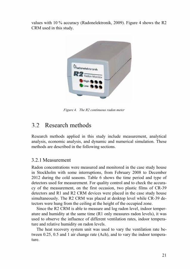
21
values with 10 % accuracy (Radonelektronik, 2009). Figure 4 shows the R2 CRM used in this study.
Figure 4. The R2 continuous radon meter
Research methods
Research methods applied in this study include measurement, analytical analysis, economic analysis, and dynamic and numerical simulation. These methods are described in the following sections.
3.2.1 Measurement Radon concentrations were measured and monitored in the case study house in Stockholm with some interruptions, from February 2008 to December 2012 during the cold seasons. Table 6 shows the time period and type of detectors used for measurement. For quality control and to check the accura-cy of the measurement, on the first occasion, two plastic films of CR-39 detectors and R1 and R2 CRM devices were placed in the case study house simultaneously. The R2 CRM was placed at desktop level while CR-39 de-tectors were hung from the ceiling at the height of the occupied zone.
Since the R2 CRM is able to measure and log radon level, indoor temper-ature and humidity at the same time (R1 only measures radon levels), it was used to observe the influence of different ventilation rates, indoor tempera-ture and relative humidity on radon levels.
The heat recovery system unit was used to vary the ventilation rate be-tween 0.25, 0.5 and 1 air change rate (Ach), and to vary the indoor tempera-ture.

22
Table 6. Date and time period of the measurements
Date Period Type of detectors Ventilation rate (Ach)
Feb, 2008 2 weeks CR-39 0.25 Jan, 2010 3 months CR-39 and R1 0.25 April, 2010 3 weeks CR-39 and R1 0.5 March, 2010 12 days R2 and R1 0.5 March, 2010 12 days R2 0.5 April, 2010 12 days R2 1 Dec, 2011 10 days R2 0.5 Dec, 2012 20 days R2 0.5
3.2.2 Analytical analysis In the case study house, the radon exhalation rate radon considered was E =65 Bqm−2h−1, and from the data regarding the house, Equation 2.5 was used to calculate indoor radon levels for different ventilation rates. This analysis was used for comparison with the results from the measurements and modeling simulation. In Equation 2.5, the factors that affect indoor ra-don are radon exhalation rate (𝐸𝐸), radon decay rate (𝜆𝜆𝑅𝑅𝑅𝑅), ventilation rate (𝜆𝜆𝑣𝑣) and height above the floor (𝐻𝐻). These factors are related according to the following equation:
𝐶𝐶𝑖𝑖 = 𝐸𝐸𝐻𝐻(𝜆𝜆𝑅𝑅𝑅𝑅+𝜆𝜆𝑣𝑣) (3.3)
In a ventilated room since 𝜆𝜆𝑅𝑅𝑅𝑅 ≪ 𝜆𝜆𝑉𝑉 the effect of the radon decay rate can be neglected. Indoor radon concentration at steady state therefore reduces to:
𝐶𝐶𝑖𝑖 = 𝐸𝐸𝐻𝐻 𝜆𝜆𝑉𝑉 (3.4)
where 𝐻𝐻 = 𝑉𝑉𝐴𝐴 = 2.4 𝑚𝑚 is the height of the case study house.
This relation clearly indicates that indoor radon concentration in a given house depends only on the air change rate and the radon exhalation rate. In this thesis this analysis is used to confirm numerical results at four distinct air change rates.
If 𝜆𝜆𝑉𝑉≅0 , equation (3.3) is reduced to:
𝐶𝐶𝑖𝑖 = 𝐸𝐸𝐻𝐻 𝜆𝜆𝑅𝑅𝑅𝑅 = 𝐶𝐶𝑚𝑚𝑚𝑚𝑚𝑚 (3.5)

23
For this case study, radon exhalation rate (𝐸𝐸) can be calculated using the maximum measured indoor radon, 𝐶𝐶𝑚𝑚𝑚𝑚𝑚𝑚 = 3580 ± 380 𝐵𝐵𝐵𝐵𝑚𝑚−3, and given 𝐻𝐻 = 2.4 m and 𝜆𝜆𝑅𝑅𝑅𝑅 =2.1× 10⁻⁶s-1, then 𝐸𝐸 = 65 ± 7 𝐵𝐵𝐵𝐵𝑚𝑚−2ℎ−1 = 18 ±2 𝑚𝑚𝐵𝐵𝐵𝐵𝑚𝑚−2𝑠𝑠−1. These values are accepted as input data in the numerical simulations and used to check sensitivity analysis.
3.2.3 Economic analysis In order to calculate the costs and energy losses imposed by the heat recov-ery unit as a radon mitigation and ventilation system and the utility costs of the residential building, the ventilation loss, operational energy cost, heat degree days, fan(s) energy use, heat energy cost, indoor air temperature and ventilation rate and initial and installation costs of the heat recovery unit must be known. Some of these factors are calculated in section 3.2.5.
3.2.4 Heating degree days (HDD) calculations Degree day values are a common and accepted method for determining the potential impact of regional climate modifications on energy demand for space heating and air conditioning. Typically, a linear relationship is as-sumed between degree days and energy consumption. In industry and aca-demia, heating and cooling degree days are a useful method which has been used for decades (Akander, Alvarez, & Johannesson, 2005). In a cold cli-mate, high heating degree days are very important from the perspective of energy recovery and multipurpose applications such as a radon mitigation ventilation system.
More specifically, heating degree days (degree hours) are a simplified means of calculating the building’s energy demand for space heating, and can be useful for example when estimating the energy saving by a heat ex-changer. The degree days depend on the location (outdoor temperature), the selected indoor temperature and the passive heat.
Consideration must be given to the contributions of passive heating (household electricity, body heat, solar radiation and heat from hot water), and it is very important that the degree days only refer to the demand for space heating, and not to the total amount of heat required to achieve the indoor temperature. This can be done by estimating the average temperature increase due to passive heating; the mean value of passive heating during the heating season divided by the building’s specific ventilation and transmis-sion heat losses per °C temperature difference between indoors and outdoors. For example, if passive heating on average contributes 3 °C of the indoor temperature increase, combined with an assumed indoor temperature of 21 °C, this means that the base temperature (limit temperature) would be 21 - 3 = 18 °C.
24
For a very well insulated building with a lot of passive heat, the low base temperature and the low degree days value will result in a much lower ener-gy saving as a result of using a heat exchanger. If the building is heated by a heat pump, it is also the case that the saving in purchased energy for active heating from using a heat exchanger will be much lower. However, these phenomena are not addressed specifically within this thesis.
Heating degree day calculations in this study were carried out using a base temperature of 18℃. Heat degree days can be calculated as follows (Mourshed, 2012):
𝐻𝐻𝐻𝐻𝐻𝐻 = ∑ ⌊𝐻𝐻𝑚𝑚 ∑ 𝑚𝑚𝑚𝑚𝑚𝑚 {𝑇𝑇𝑏𝑏 − 𝑇𝑇𝑑𝑑, (0.0)}⌋12𝑚𝑚=1 (3.6)
𝐻𝐻𝐻𝐻𝐻𝐻 = 𝑇𝑇𝑏𝑏 − 𝑇𝑇𝑑𝑑 if 𝑇𝑇𝑑𝑑 < 𝑇𝑇𝑏𝑏
𝐻𝐻𝐻𝐻𝐻𝐻 = 0 if 𝑇𝑇𝑑𝑑 ≥ 𝑇𝑇𝑏𝑏
where 𝐻𝐻𝑚𝑚 is the number of days in month 𝑚𝑚, 𝑇𝑇𝑑𝑑 is the daily mean tempera-ture and 𝑇𝑇𝑏𝑏 is the base temperature.
3.2.5 Ventilation loss This section considers the “theoretical” portion of the space heating that compensates for ventilation losses. It is assumed that the fan-driven supply air flow represents 90 % of the fan-driven exhaust air flow (a normal ratio leading to a small negative average indoor pressure, which is an advantage with regards to humidity), temperature efficiency for the heat exchanger is 74.5 %, and air leakage in addition to fan-driven ventilation is equal to 0.05 Ach.
The heat exchanger only affects the fan-driven supply air (90 % of the exhaust air):
0.90𝜆𝜆𝑣𝑣 × 𝑉𝑉 = 0.90 × 0.5 𝐴𝐴𝐴𝐴ℎ × 259 𝑚𝑚3 = 116.55 𝑚𝑚3ℎ−1
where 𝜆𝜆𝑣𝑣 = air change ventilation rate, 𝑉𝑉 = building effective volume (m3). Total infiltration (air leakage) not affected by the heat exchanger is the
sum of the fan-driven infiltration (10 % of the exhaust air flow) and the air leakage (0.05 Ach) corresponding to air leakage both in and out in addition to fan-driven ventilation (Oman, 2011; Mourshed, 2012), i.e. 0.10 ×0.5 𝐴𝐴𝐴𝐴ℎ × 259𝑚𝑚3 + 0.05 𝐴𝐴𝐴𝐴ℎ × 259𝑚𝑚3 = 25.9 𝑚𝑚3ℎ−1
Specific ventilation loss (𝑄𝑄𝑣𝑣) is defined as:
𝑄𝑄𝑣𝑣 = Fan − driven supply air + total infiltration
25
𝑄𝑄𝑣𝑣 = ∑ m𝐶𝐶𝑝𝑝 (3.7)
where 𝐶𝐶𝑝𝑝 = air heat capacity (1,010 J.kg-1°C-1) and m= mass flow 𝑘𝑘𝑘𝑘𝑠𝑠−1.
𝑄𝑄𝑣𝑣 = 0.039 × 1,010 + 0.0086 × 1,010 = 39.39 + 8.69 = 48.09 𝑊𝑊°𝐶𝐶−1
Ventilation losses (𝐸𝐸𝑣𝑣), which is defined as the sum of fan-driven supply air (𝐸𝐸𝑠𝑠) and total infiltration (𝐸𝐸𝑙𝑙) losses, is calculated from the basic equation
𝑄𝑄 = m𝐶𝐶𝑇𝑇:𝐸𝐸𝑣𝑣 = 𝐸𝐸𝑠𝑠 + 𝐸𝐸𝑙𝑙 = 𝑄𝑄𝑣𝑣 × 24 × 𝐻𝐻𝐻𝐻𝐻𝐻 (3.8)
where 𝐸𝐸𝑠𝑠 = the specific portion of the space heating in Wh/year required to compensate for the heat losses caused by the fan-driven supply air, El = the specific portion of the space heating in Wh/year required to compensate for the heat losses caused by the total infiltration (air leakage) not affected by the heat exchanger, and 24 × 𝐻𝐻𝐻𝐻𝐻𝐻 = heat degree hours per year.
Based on monthly long-term mean temperatures in Stockholm, the heat-ing degree days are estimated to be about 4,500 degree days (108,000 heat degree hours per year (Wunderground, 2010).
The heat exchanger reduces the heat demand by a factor (1–t). The ener-gy demand of heating using heat exchanger (EHex ) is:
EHex = Es (1 –𝑡𝑡) (3.9)
Recovered heat loss (𝐸𝐸𝑟𝑟𝑟𝑟𝑟𝑟 in Wh/year) comes directly from the following expression:
𝐸𝐸𝑟𝑟𝑟𝑟𝑟𝑟 = 𝐸𝐸𝑆𝑆 − 𝐸𝐸𝐻𝐻𝑟𝑟𝐻𝐻 = 𝑡𝑡Es (3.10)
If we consider the normal ranges of variation of each variable as
0.5 ≤ 𝜆𝜆𝑣𝑣 ≤ 1; 4,000 ≤ 𝐻𝐻𝐻𝐻𝐻𝐻 ≤ 6,000; and 0.7 ≤ 𝜂𝜂𝑡𝑡 ≤ 0.85,
the annual energy recovery can be determined.
3.2.6 The life cycle cost analysis of heat recovery ventilation system
The net present value (NPV) method is a method used to evaluate the cost-effectiveness of an investment in the future. According to this method, an

26
investment is profitable if the net present value (B0) of all savings is larger than the capital initial cost (A0), as shown in Equation 3.11 (Nilsson, 2006).
B0 > A0 (3.11)
where A0= initial investment and B0 = NPV of all savings, which is defined as:
B0 = Ib (3.12)
where b = Annual savings in monetary unit, and I = NPV factor which is expressed as:
𝐼𝐼 = 1−(1+𝑖𝑖)−𝑛𝑛
𝑖𝑖 (3.13)
where 𝑖𝑖 = interest rate, and n= time in years. Taking into account the annual increases in the energy price, a new NPV
factor 𝐼𝐼𝑞𝑞 can be calculated (Nilsson, 2006):
𝐼𝐼𝑞𝑞 = 1−(1+𝑞𝑞1+𝑖𝑖 )
𝑛𝑛
1+𝑖𝑖1+𝑞𝑞−1
(3.14)
where q = annual energy cost escalation rate = 2 % and I = annual interest rate = 4 % (Nilsson, 2006).
In the present study, NPV analysis is used to show whether the invest-ment to install a heat recovery system is cost-effective or not. This analysis, presented in section 5.4 and Paper I, shows that installing an air handling unit is useful and cost-effective because it both reduces energy costs and mitigates indoor radon levels.
Energy dynamic simulation
For a long term assessment of the heat recovery ventilation efficiency, a complete time series of outdoor temperature and all building losses and gains during the heating period should be considered. The variations of outdoor temperature and ventilation rate may change the heat recovery temperature and humidity efficiencies. All these time dependent effects are taken into account using energy dynamic programs. The IDA Indoor Climate and En-ergy (IDA ICE) energy dynamic program used in this study is a multi-zone dynamic simulation software package used to study thermal indoor climate
27
and predict energy consumption of the whole building, heat recovery of the rotary heat exchanger unit analysis, simulate thermal comfort and IAQ.
The case study house is considered as a building with 8 zones. Energy and heat are provided by a primary source and a balanced heat recovery unit. Weather data is taken from a database of the Stockholm climate. Boundary conditions and input data used in this simulation are listed in Appendix A.
Computational fluid dynamics (CFD)
CFD analysis is used to investigate the effects of indoor air parameters on indoor radon treatment numerically. CFD can be easily used for indoor air flow analysis, and reduces the mathematical limitations. It is also more cost-effective than full-scale laboratory and tracer gas methods. CFD programs are designed to solve the governing equations in the form of partial differen-tial equations (PDE), and are employed to solve equations involving veloci-ty, temperature and species transport numerically. In a room with ventilation, CFD programs are able to describe the processes in the room, including the conservation of mass, energy, momentum and species such as radon. The reasons for using CFD and the finite volume method (FVM) are described in greater detail in the next chapter.

28

29
4 Numerical Modeling Procedure
In order to visualize the progress of the behavior of fluid flow and indoor radon and air conditions effects, the conservation of mass, energy, momen-tum and species transport in the flow field must be defined. The resulting governing equations are PDE which include several independent variables and their partial derivatives.
There are different approaches for solving PDE. One such approach is numerical solution using CFD. CFD code is designed to solve PDE numeri-cally. The CFD codes convert PDE from continuous equations to discrete equations (algebraic equations) based on different discretization methods.
Discretization methods
In fluid dynamics, the major discretization methods are Finite Volume Method (FVM), Finite Difference Method (FDM) and Finite Element Meth-od (FEM).
Unlike the analytical solution, which solves the equations for all points in the domain, the numerical methods support only discrete points (nodes) and values are calculated at discrete locations on a meshed geometry. The crea-tion of the geometry and mesh is the first pre-processing step in numerical modeling. The shape of these cells in 3-D is usually polyhedral (tetrahedral, hexahedral, prism, etc.).
The FDM uses the differential forms of the governing equations and ap-plies the local Taylor series expansion to approximate differential equations, whereas the FVM and FEM use the integral form of the governing equations. The FEM divides complicated equations into small elements that can be solved in relation to each other. Solving the problems with the FEM method typically needs more computer memory compared to the FVM (Motaman, 2013). The main advantage of FVM is that it can be used with unstructured grids. In this method the computational domain is divided into small vol-umes, and variables of a problem such as velocity, temperature, and species, etc. are placed at the centroid of the control volume rather than at nodal points. The values of field variables at vertices are obtained by interpolation. Volume integrals are then converted to surface integrals using the diver-gence theorem. These terms are then calculated as fluxes across volume sur-

30
faces of each finite volume, because the flux entering a given volume is identical to that leaving the adjacent volume. These methods are called con-servative (Abd Alnasser Almate A., 2014).
FLUENT is a powerful commercial CFD code which uses FVM to solve partial differential equations and has been widely used for indoor air flow problems. FLUENT is thus used in this study.
4.1.1 Finite control volume analysis The conservation law is used in FVM to solve numerical equations. The general conservation form of fluid flow for a small control volume of a de-pendent variable (𝐶𝐶) may be written as:
𝜕𝜕(𝜌𝜌𝜌𝜌)𝜕𝜕𝜕𝜕 + 𝑑𝑑𝑑𝑑𝑑𝑑 (𝜌𝜌𝐶𝐶𝑽𝑽) = 𝑑𝑑𝑑𝑑𝑑𝑑 (𝜌𝜌𝜌𝜌 𝑔𝑔𝑔𝑔𝑔𝑔𝑑𝑑𝐶𝐶) + 𝑆𝑆𝜌𝜌 (4.1)
This equation has 4 terms. From the left: the first term states the time rate change of the fluid element of the variable(𝐶𝐶), this is the so-called unsteady effect; the second term is the net rate of flow (𝐶𝐶) out of the fluid element, this is because of the advection (motion) effect; the third term is the change rate of 𝐶𝐶 due to the diffusion effect; and the final term is the source term, which is the change rate of fluid flow due to generation. In this study the governing equations are presented in the form of Equation 4.1.
In the FVM, the conservation law is applied to each finite element at which the computation of the flux across the boundary is required. The fol-lowing steps are undertaken for solving PDE in this method. The first step is conversion of each volume integral of the PDE to a surface integral using the divergence theorem. The second step is integration of the differential form of the PDE over each volume. The conservation equations for each volume may be solved simultaneously. In the third step, surface integrals are con-verted to algebraic equations using mean value theorem. In the final step the algebraic equations are converted to matrices, which can then be solved by the iteration method.
Governing equations used
The governing equations for this study are conservation of mass (continuity), momentum (Navier-Stokes equations), and energy, and concentration of species equations are generally referred to as transport equations. To find all unknown variables (pressure, velocity components, temperature), another equation called the state equation is needed.
Air flow in a room is incompressible due to the low indoor air velocity, which is in the order of less than 1 meter per second. For an incompressible
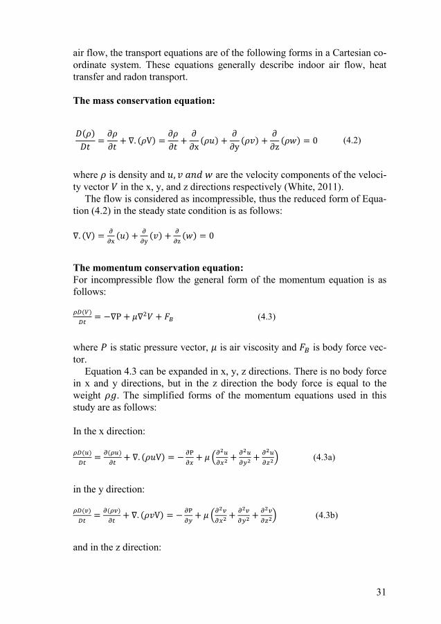
31
air flow, the transport equations are of the following forms in a Cartesian co-ordinate system. These equations generally describe indoor air flow, heat transfer and radon transport.
The mass conservation equation:
𝐷𝐷(𝜌𝜌)𝐷𝐷𝐷𝐷 = 𝜕𝜕𝜌𝜌
𝜕𝜕𝐷𝐷 + ∇. (𝜌𝜌V) = 𝜕𝜕𝜌𝜌𝜕𝜕𝐷𝐷 + ∂
∂x (𝜌𝜌𝜌𝜌) + ∂∂y (𝜌𝜌𝜌𝜌) + ∂
∂z (𝜌𝜌𝜌𝜌) = 0 (4.2)
where 𝜌𝜌 is density and 𝜌𝜌, 𝜌𝜌 𝑎𝑎𝑎𝑎𝑎𝑎 𝜌𝜌 are the velocity components of the veloci-ty vector 𝑉𝑉 in the x, y, and z directions respectively (White, 2011).
The flow is considered as incompressible, thus the reduced form of Equa-tion (4.2) in the steady state condition is as follows:
∇. (V) = ∂∂x (𝜌𝜌) + ∂
∂y (𝜌𝜌) + ∂∂z (𝜌𝜌) = 0
The momentum conservation equation: For incompressible flow the general form of the momentum equation is as follows:
𝜌𝜌𝜌𝜌(𝑉𝑉)𝜌𝜌𝐷𝐷 = −∇P + 𝜇𝜇∇2𝑉𝑉 + 𝐹𝐹𝐵𝐵 (4.3)
where 𝑃𝑃 is static pressure vector, 𝜇𝜇 is air viscosity and 𝐹𝐹𝐵𝐵 is body force vec-tor.
Equation 4.3 can be expanded in x, y, z directions. There is no body force in x and y directions, but in the z direction the body force is equal to the weight 𝜌𝜌𝑔𝑔. The simplified forms of the momentum equations used in this study are as follows:
In the x direction:
𝜌𝜌𝜌𝜌(𝑢𝑢)𝜌𝜌𝐷𝐷 = 𝜕𝜕(𝜌𝜌𝑢𝑢)
𝜕𝜕𝐷𝐷 + ∇. (𝜌𝜌𝜌𝜌V) = − 𝜕𝜕P𝜕𝜕𝜕𝜕 + 𝜇𝜇 (𝜕𝜕2𝑢𝑢
𝜕𝜕𝜕𝜕2 + 𝜕𝜕2𝑢𝑢𝜕𝜕𝑦𝑦2 + 𝜕𝜕2𝑢𝑢
𝜕𝜕𝑧𝑧2) (4.3a)
in the y direction:
𝜌𝜌𝜌𝜌(𝑣𝑣)𝜌𝜌𝐷𝐷 = 𝜕𝜕(𝜌𝜌𝑣𝑣)
𝜕𝜕𝐷𝐷 + ∇. (𝜌𝜌𝜌𝜌V) = − 𝜕𝜕P𝜕𝜕𝑦𝑦 + 𝜇𝜇 (𝜕𝜕2𝑣𝑣
𝜕𝜕𝜕𝜕2 + 𝜕𝜕2𝑣𝑣𝜕𝜕𝑦𝑦2 + 𝜕𝜕2𝑣𝑣
𝜕𝜕𝑧𝑧2) (4.3b)
and in the z direction:

32
𝜌𝜌𝜌𝜌(𝑤𝑤)𝜌𝜌𝐷𝐷 = 𝜕𝜕(𝜌𝜌𝑤𝑤)
𝜕𝜕𝐷𝐷 + ∇. (𝜌𝜌𝜌𝜌V) = − 𝜕𝜕P𝜕𝜕𝜕𝜕 + 𝜇𝜇 (𝜕𝜕2𝑤𝑤
𝜕𝜕𝑥𝑥2 + 𝜕𝜕2𝑤𝑤𝜕𝜕𝑦𝑦2 + 𝜕𝜕2𝑤𝑤
𝜕𝜕𝜕𝜕2 ) + 𝜌𝜌𝑔𝑔 (4.3c)
where 𝑝𝑝 is the static pressure, 𝜇𝜇 is the viscosity of the air, i.e. 1.83×10⁻⁵ kgm-
1s-1 at T = 293 K, and 𝑔𝑔 is acceleration due to gravity (White, 2011).
The energy conservation equation: The general form of the energy conservation equation of indoor incompress-ible air is:
𝜕𝜕(𝜌𝜌𝐶𝐶𝑝𝑝𝑇𝑇)𝜕𝜕𝐷𝐷 + ∇. (𝜌𝜌𝐶𝐶𝑝𝑝𝑇𝑇𝑽𝑽) = ∇. (𝑘𝑘∇𝑇𝑇) + 𝑆𝑆𝑒𝑒 (4.4)
In this study the following reduced form is used:
∇. (𝜌𝜌𝐶𝐶𝑝𝑝𝑇𝑇𝑽𝑽) = ∇. (𝑘𝑘∇𝑇𝑇)
where 𝐶𝐶𝑝𝑝 is the specific heat capacity of the air, 𝑘𝑘 is the thermal conductivi-ty, and 𝑆𝑆𝑒𝑒 is energy source, which is zero in this case (White, 2011).
Radon transport equation: Theoretical and mathematical relations indicate that diffusion and advection mechanisms2 lead to radon transport (Spoel, 1998). Advection mechanisms are more related to physical and environmental conditions such as air flow, ventilation rate, indoor temperature, relative humidity and pressure differ-ences between indoors, the ground and the outdoors.
The general form of the radon mass transfer equation, like Equation (4.1) referred to as the total radon transport equation, integrates radon diffusion transport, advection transport, radon generation and radon decay rate. In steady state and incompressible flow it is written as the following conserva-tion equation (Wang & Ward, 2000):
𝑑𝑑𝐶𝐶𝑑𝑑𝐷𝐷 = 𝛻𝛻. (𝐷𝐷𝛻𝛻𝐶𝐶) + 𝛻𝛻. 𝐶𝐶𝑽𝑽 − 𝜆𝜆𝑅𝑅𝑅𝑅𝐶𝐶 + 𝐺𝐺 = 0 (4.5)
where 𝐷𝐷 = Radon diffusion coefficient in air(𝑚𝑚2𝑠𝑠−1), and 𝐶𝐶 = Radon activi-ty concentration in air(𝐵𝐵𝐵𝐵 𝑚𝑚−3).
𝐺𝐺 = Radon generation rate(𝐵𝐵𝐵𝐵 𝑚𝑚−3𝑠𝑠−1), 𝑽𝑽 is the velocity vector and 𝜆𝜆𝑅𝑅𝑅𝑅 = 2.1 × 10⁻⁶𝑠𝑠−1 .
2 Diffusion is driven by concentration gradient and advection is due to pressure difference caused by mechanical ventilation. Note that advection is fluid motion due to fluid stream, but convection used for heat transfer includes both diffusion and advection.

33
In a room air flow, the dominant driving force is the advection force caused by physical and environmental conditions such as wind, rainfall, stack effect, temperature, relative humidity and mechanical ventilation sys-tems or combinations of these. If the dominant source is diffusion, such as during migration in soil, a different transport equation would apply. This equation and some points related to this issue are explained in Appendix B.
As mentioned for Equation 4.1, the radon transport equation can be writ-ten in a general form as:
𝜕𝜕(𝜌𝜌𝜌𝜌)𝜕𝜕𝜕𝜕 + 𝑑𝑑𝑑𝑑𝑑𝑑(𝜌𝜌𝜌𝜌𝜌𝜌) = 𝑑𝑑𝑑𝑑𝑑𝑑(𝜌𝜌𝜌𝜌 𝑔𝑔𝑔𝑔𝑎𝑎𝑑𝑑(𝜌𝜌)) + 𝑆𝑆𝜌𝜌 (4.6)
In the above expression, 𝑆𝑆𝜌𝜌 is the source term and V is the velocity vector, ρ is the density of the radon and D is the diffusion coefficient. Here, since radon is transported to the air and there is no radon generation and decay in the air, 𝑆𝑆𝜌𝜌 = 0 and the equation reduces to:
𝜕𝜕(𝜌𝜌𝜌𝜌)𝜕𝜕𝜕𝜕 + 𝑑𝑑𝑑𝑑𝑑𝑑(𝜌𝜌𝜌𝜌𝜌𝜌) = 𝑑𝑑𝑑𝑑𝑑𝑑(𝜌𝜌𝜌𝜌 𝑔𝑔𝑔𝑔𝑎𝑎𝑑𝑑(𝜌𝜌)) (4.7)
For steady state conditions and constant radon density, Equation 4.7 reduces to
𝑑𝑑𝑑𝑑𝑑𝑑(𝜌𝜌𝜌𝜌) = 𝑑𝑑𝑑𝑑𝑑𝑑(𝜌𝜌 𝑔𝑔𝑔𝑔𝑎𝑎𝑑𝑑(𝜌𝜌)) (4.8)
In two dimensions, the differential form of this equation becomes
𝜕𝜕(𝜌𝜌𝐶𝐶)𝜕𝜕𝜕𝜕 + 𝜕𝜕(𝜌𝜌𝐶𝐶)
𝜕𝜕𝜕𝜕 = 𝜕𝜕𝜕𝜕𝜕𝜕 (𝜌𝜌 𝜕𝜕𝜌𝜌
𝜕𝜕𝜕𝜕) + 𝜕𝜕𝜕𝜕𝜕𝜕 (𝜌𝜌 𝜕𝜕𝜌𝜌
𝜕𝜕𝜕𝜕) (4.9)
Integration of Equation 4.8 over a three dimensional control volume CV yields
∫ 𝑑𝑑𝑑𝑑𝑑𝑑(𝜌𝜌𝜌𝜌) 𝜌𝜌𝐶𝐶 𝑑𝑑∀= ∫ 𝑑𝑑𝑑𝑑𝑑𝑑(𝜌𝜌 𝑔𝑔𝑔𝑔𝑎𝑎𝑑𝑑(𝜌𝜌))
𝜌𝜌𝐶𝐶 𝑑𝑑∀ (4.10)
The left hand term (the convective term) and the right hand term (the diffu-sion term) are re-written as integrals over the entire bounding surface of the control volume by using divergence theorem (Versteeg & Malalasekera, 2007).
The complete description and discretization form of the indoor radon transport equation lies outside of the scope of this thesis. The interested reader is referred to (Bakker, 2010) for more information on the subject.
In addition to these governing equations, because the turbulence model is used in this study, two additional transport equations of turbulent energy
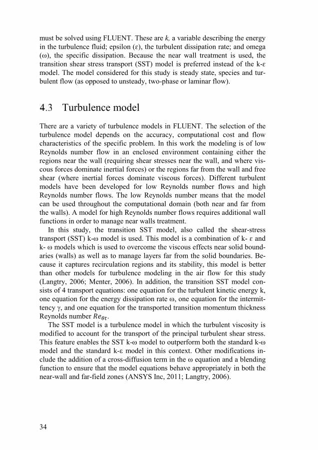
34
must be solved using FLUENT. These are k, a variable describing the energy in the turbulence fluid; epsilon (ɛ), the turbulent dissipation rate; and omega (ω), the specific dissipation. Because the near wall treatment is used, the transition shear stress transport (SST) model is preferred instead of the k-ɛ model. The model considered for this study is steady state, species and tur-bulent flow (as opposed to unsteady, two-phase or laminar flow).
Turbulence model
There are a variety of turbulence models in FLUENT. The selection of the turbulence model depends on the accuracy, computational cost and flow characteristics of the specific problem. In this work the modeling is of low Reynolds number flow in an enclosed environment containing either the regions near the wall (requiring shear stresses near the wall, and where vis-cous forces dominate inertial forces) or the regions far from the wall and free shear (where inertial forces dominate viscous forces). Different turbulent models have been developed for low Reynolds number flows and high Reynolds number flows. The low Reynolds number means that the model can be used throughout the computational domain (both near and far from the walls). A model for high Reynolds number flows requires additional wall functions in order to manage near walls treatment.
In this study, the transition SST model, also called the shear-stress transport (SST) k-ω model is used. This model is a combination of k- ɛ and k- ω models which is used to overcome the viscous effects near solid bound-aries (walls) as well as to manage layers far from the solid boundaries. Be-cause it captures recirculation regions and its stability, this model is better than other models for turbulence modeling in the air flow for this study (Langtry, 2006; Menter, 2006). In addition, the transition SST model con-sists of 4 transport equations: one equation for the turbulent kinetic energy k, one equation for the energy dissipation rate , one equation for the intermit-tency , and one equation for the transported transition momentum thickness Reynolds number 𝑅𝑅𝑅𝑅𝜃𝜃𝜃𝜃.
The SST model is a turbulence model in which the turbulent viscosity is modified to account for the transport of the principal turbulent shear stress. This feature enables the SST k-ω model to outperform both the standard k-ω model and the standard k-ε model in this context. Other modifications in-clude the addition of a cross-diffusion term in the ω equation and a blending function to ensure that the model equations behave appropriately in both the near-wall and far-field zones (ANSYS Inc, 2011; Langtry, 2006).

35
Boundary conditions and input data
Since simulations are performed for Sweden – and specifically for a de-tached house located in Stockholm – values and constants are set specifically for this geographical location. These values vary with the time of year. For example, the maximum radon exhalation rate occurs in July due to the envi-ronmental conditions. Since measurements were taken from December through March, the average radon exhalation rate through these months is used. Some values, such as wind speed and indoor/outdoor temperature, are taken from the data included in IDA ICE.
The radon exhalation rate in the case study house is based on measured data and calculation with Equation (3.5): E = 0.018 Bqm-2s-1.
The following sub-sections explain the boundary conditions and input da-ta which have been used in the model.
4.4.1 Inlet Vent The supply air terminal device in the room is the fresh air supplier. This boundary is defined as “Velocity Inlet” in the model. Specifications which must be defined for this boundary are “Velocity magnitude and hydraulic diameter”, turbulence specifications including “Intermittency”, “Turbulent intensity”, “Static temperature”, and species mass fractions including “Mass fraction of radon” and “Mass fraction of water vapor”.
1. Velocity magnitude and hydraulic diameter: The supply air terminal device size is 20 cm × 30 cm. The hydraulic diam-eter of the supply air terminal device can be calculated as follows
𝐷𝐷ℎ,𝑉𝑉𝑉𝑉𝑉𝑉𝑉𝑉 = 4𝐴𝐴𝑃𝑃 = 4×30×20
2(20+30) = 24 𝑐𝑐𝑐𝑐 𝑜𝑜𝑜𝑜 0.24 𝑐𝑐
In all cases, supply air terminal device size and therefore hydraulic diame-ter is constant.
Calculations are carried out for several air change rates which are listed in Table 9. For each air change rate, the velocity at the supply air terminal device is calculated from the following expression:
𝑉𝑉𝑉𝑉𝑉𝑉𝑉𝑉𝑉𝑉 = 𝐴𝐴𝐴𝐴ℎ×𝑉𝑉𝑉𝑉𝑉𝑉𝑉𝑉𝑉𝑉𝑉𝑉𝑅𝑅𝑅𝑅𝑅𝑅𝑅𝑅𝐴𝐴𝐴𝐴𝑉𝑉𝐴𝐴𝑉𝑉𝑉𝑉𝑉𝑉𝑉𝑉
For example for Ach = 0.5 hr-1, velocity at supply air terminal device (vent) is
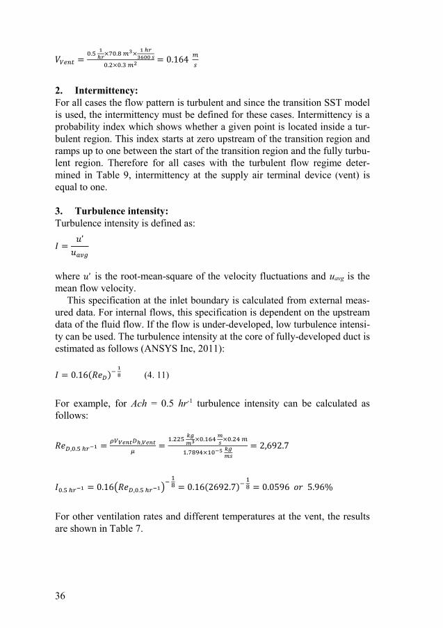
36
𝑉𝑉𝑉𝑉𝑉𝑉𝑉𝑉𝑉𝑉 = 0.5 1ℎ𝑟𝑟×70.8 𝑚𝑚3× 1 ℎ𝑟𝑟
3600 𝑠𝑠0.2×0.3 𝑚𝑚2 = 0.164 𝑚𝑚
𝑠𝑠
2. Intermittency: For all cases the flow pattern is turbulent and since the transition SST model is used, the intermittency must be defined for these cases. Intermittency is a probability index which shows whether a given point is located inside a tur-bulent region. This index starts at zero upstream of the transition region and ramps up to one between the start of the transition region and the fully turbu-lent region. Therefore for all cases with the turbulent flow regime deter-mined in Table 9, intermittency at the supply air terminal device (vent) is equal to one.
3. Turbulence intensity: Turbulence intensity is defined as:
𝐼𝐼 = 𝑢𝑢’𝑢𝑢𝑎𝑎𝑎𝑎𝑎𝑎
where 𝑢𝑢’ is the root-mean-square of the velocity fluctuations and uavg is the mean flow velocity.
This specification at the inlet boundary is calculated from external meas-ured data. For internal flows, this specification is dependent on the upstream data of the fluid flow. If the flow is under-developed, low turbulence intensi-ty can be used. The turbulence intensity at the core of fully-developed duct is estimated as follows (ANSYS Inc, 2011):
𝐼𝐼 = 0.16(𝑅𝑅𝑅𝑅𝐷𝐷)− 18 (4. 11)
For example, for Ach = 0.5 hr-1 turbulence intensity can be calculated as follows:
𝑅𝑅𝑅𝑅𝐷𝐷,0.5 ℎ𝑟𝑟−1 = 𝜌𝜌𝑉𝑉𝑉𝑉𝑉𝑉𝑉𝑉𝑉𝑉𝐷𝐷ℎ,𝑉𝑉𝑉𝑉𝑉𝑉𝑉𝑉𝜇𝜇 =
1.225 𝑘𝑘𝑘𝑘𝑚𝑚3×0.164 𝑚𝑚𝑠𝑠 ×0.24 𝑚𝑚
1.7894×10⁻⁵ 𝑘𝑘𝑘𝑘𝑚𝑚𝑠𝑠
= 2,692.7
𝐼𝐼0.5 ℎ𝑟𝑟−1 = 0.16(𝑅𝑅𝑅𝑅𝐷𝐷,0.5 ℎ𝑟𝑟−1)− 18 = 0.16(2692.7)− 18 = 0.0596 𝑜𝑜𝑜𝑜 5.96%
For other ventilation rates and different temperatures at the vent, the results are shown in Table 7.

37
Table 7. Velocity and turbulence intensity for different ventilation rates
Ach (hr-1) VVent (ms-1) ReD I (%) 0.05 0.017 - - 0.25 0.082 1,346.4 6.50 0.5 0.164 2,692.7 5.96 1.0 0.328 5,385.4 5.46
4. Species mass fractions: Mass fraction of each species must also be determined at this boundary (the inlet vent). Since a supply air terminal device is used as fresh air supplier, the mass fraction of radon at this boundary is zero. The mass fraction of water vapor must be determined according to relative humidity and tempera-ture. Calculations for determining mass fraction of water vapor have been carried out and are presented in section 4.8. These same calculations can be used here. The sum of the mass fractions of all species must be equal to one. Therefore the mass fraction of air is obtained by subtracting the mass frac-tions of radon and water vapor from 1.0.
4.4.2 Outlet All supply air from the rooms leaves the house through the unique outlet. Due to the geometrical conditions (Figure 5), supply air from Room 1 exits this room through the air holes of internal Door 1 (all internal doors are sup-posed to be closed). Therefore, the outlet for Room 1 is located on internal Door 1 (Figure 6).
Since there is one outlet, this boundary is defined as an outflow and con-sequently its flow rate weighting is one. Considering outflow also helps the model achieve quick convergence.
4.4.3 Outer Surfaces Outer surfaces are exposed to the outdoor air conditions. These surfaces include the outer lateral walls, the roof, the window and the main door. The same boundary conditions are used for each of these surfaces (however ac-cording to Section 4.7, the appropriate material and thickness must be used for each component). Wall with convection heat transfer was shown empiri-cally to model these boundaries appropriately. Therefore outdoor air temper-ature and convective heat transfer coefficient (CHTC) must be defined.
According to results from IDA ICE (Appendix A), average outdoor air temperature and wind speed in Stockholm from December to March are -2 °C and 2.5 ms-1 respectively.
Flow around buildings is highly complicated, since it is defined by im-pinging flow, separating flow, reattaching flow, circulating flow, vortexes,

38
etc. It is therefore difficult to calculate CHTC using simple equations. However, several correlations have been presented for calculating CHTC.
In this study the following expression is used for CHTC (Shao, 2010):
𝐶𝐶𝐶𝐶𝐶𝐶𝐶𝐶 ( 𝑊𝑊𝑚𝑚2𝐾𝐾) = 4.2 𝑉𝑉 (𝑚𝑚
𝑠𝑠 ) + 6.01 (4.12)
where V is the wind speed of outdoor air.
Using this equation gives:
𝐶𝐶𝐶𝐶𝐶𝐶𝐶𝐶 = 4.2 × 2.5 + 6.01 = 16.5 ( 𝑊𝑊𝑚𝑚2𝐾𝐾)
4.4.4 Internal Surfaces Internal surfaces include the internal walls and the internal doors (Door 1, Door 2 and Door 3). Since indoor temperature is considered as uniform, heat transfer through these surfaces can be neglected, thus these boundaries are considered as wall with zero heat flux.
4.4.5 Floor Zone This study investigates effective parameters (including ventilation rate, tem-perature and relative humidity) for controlling indoor radon concentration in a specific range. Soil is therefore not modeled, and radon exhalation rate from the measurements from this specific geographical location and time period are used to determine radon entry rate into the room. Radon entry into the room is modeled through generation of radon in the floor. Therefore, the floor is modeled as a porous zone with a specific radon generation rate. Po-rous zone features of the floor do not have any bearing on the results. Radon generation rate (𝐺𝐺𝑅𝑅𝑅𝑅𝑅𝑅𝑅𝑅𝑅𝑅) in the floor for Room 1 can be obtained as follows:
��𝑚𝑅𝑅𝑅𝑅𝑅𝑅𝑅𝑅𝑅𝑅 = 𝐸𝐸 × 𝐴𝐴𝐴𝐴𝐴𝐴𝐴𝐴𝐹𝐹𝐹𝐹𝑅𝑅𝑅𝑅𝑜𝑜 = 0.018 𝐵𝐵𝐵𝐵𝑚𝑚2𝑠𝑠 × 29.5 𝑚𝑚2 = 0.53 𝐵𝐵𝐵𝐵
𝑠𝑠
𝐺𝐺𝑅𝑅𝑅𝑅𝑅𝑅𝑅𝑅𝑅𝑅 = ��𝑚𝑅𝑅𝑅𝑅𝑅𝑅𝑅𝑅𝑅𝑅𝑉𝑉𝑅𝑅𝐹𝐹𝑉𝑉𝑚𝑚𝑉𝑉𝐹𝐹𝐹𝐹𝑅𝑅𝑅𝑅𝐹𝐹
=0.53 𝐵𝐵𝐵𝐵
𝑠𝑠 ×(1.75×10⁻¹⁹ 𝑘𝑘𝑘𝑘𝐵𝐵𝐵𝐵)
0.295 𝑚𝑚3 = 3.2 × 10⁻¹⁹ 𝑘𝑘𝑘𝑘𝑚𝑚3𝑠𝑠
Radon generation rate must be converted to SI units for use in FLUENT. Conversion is done by multiplication based on the following conversion factor (Wang & Ward, 2000):
1 𝐵𝐵𝐵𝐵 = 1.75 × 10⁻¹⁹ 𝑘𝑘𝑘𝑘 (4.13)

39
The House Plan Geometry
The house plan geometry is shown in Figure 5. The house plan consists of 8 rooms. Each room has its own vent. Radon enters the house through the floor. The radon entry rate into the house is determined based on the radon exhalation rate for the geographical location. A heat exchanger unit is placed in Room 4. Here the effect of the heat exchanger is ignored and it is replaced by an outlet vent located in Room 4 to play the role of the heat exchanger. The air change rate in each room corresponds to the volume of that room, and all inlet air from the rooms passes through the unique outlet.
Figure 5. The house plan geometry
Room 1 is the sitting room and is therefore very important from the view point of radon concentration. This room is thus considered for analysis and conclusion. The Geometry of Room 1 is shown in Figure 6. In this geometry all internal doors (Door 1, Door 2 and Door 3) are closed. The Main Door and Window are also closed and are exposed to the outdoor air. The supply air leaves the room through the air holes. Figure 6 show that all supply air from the rooms leaves the house through the unique outlet. Therefore supply air from Room 1 exits from this room through the air holes of internal Door 1. In other words, Room 1 is considered to have one outlet located on inter-nal Door 1 (Figure 6).

40
Radon enters Room 1 through the floor. Radon entry rate into the room is determined from the radon exhalation rate.
Figure 6. Room1 geometry
The Floor area is 29.5 m2 and the supply air terminal device area is 0.06 m2. The height of the room is 2.4 m and the volume 70.8 m3.
The dimensions of the house elements are summarized in Table 8.
Table 8. Sizes of the building elements
Elements Size (m) Thickness (m)
Window 2.5×2.2 0.025
Main Door 1.5×2.2 0.05
Internal Doors
1×2.2 0.02
External walls
- 0.03
Roof - 0.03
Parameters Variation Range
This study considers variations in three parameters, and examines the effects of changes in these parameters on indoor radon content. The parameters are

41
air change rate, temperature and relative humidity. Considered values of air change rate are 0.05, 0.25, 0.5 and 1.0 hr-1; the temperature ranges from 15 °C to 25°C; and relative humidity ranges are between 30 % and 80 % (Paper III, IV). 13 cases within these ranges are defined the studies as shown in Table 9.
Table 9. Different cases studied in this work
Temperature changes Relative humidity changes Ventilation rate changes
Case No.
Parameters Case No.
Parameters Case No.
Parameters
N1 Ach=0.5 hr-1, T=15 °C, RH=40%
N6 Ach=0.5 hr-1, T=21 °C, RH=30%
N11 Ach=1.0 hr-1, T=21 °C, RH=40%
N2 Ach=0.5 hr-1, T=18 °C, RH=40%
N3 Ach=0.5 hr-1, T=21 °C, RH=40%
N3 Ach=0.5 hr-1, T=21 °C, RH=40%
N3 Ach=0.5 hr-1, T=21 °C, RH=40%
N7 Ach=0.5 hr-1, T=21 °C, RH=50%
N12 Ach=0.25 hr-1, T=21 °C, RH=40%
N4 Ach=0.5 hr-1, T=23 °C, RH=40%
N8 Ach=0.5 hr-1, T=21 °C, RH=60%
N13 Ach=0.05 hr-1, T=21 °C, RH=40%
N5 Ach=0.5 hr-1, T=25 °C, RH=40%
N9 Ach=0.5 hr-1, T=21 °C, RH=70%
- -
- - N10 Ach=0.5 hr-1, T=21 °C, RH=80%
- -
Materials Properties
Materials used in the model are air, water vapor and radon as fluids; light concrete for the floor, dense concrete for the walls and the roof, window material, main door material and internal door material as solids. Properties of these materials are shown in Tables 10 and 11 for fluids and solids respec-tively.

42
Table 10. Properties of the fluids (Lide, 2004)
Property Radon Water vapor Air Density (kgm-3) 9.73 0.554 1.225
Heat capacity (Jkg-1K-1)
93.55 2,014 1,006.43
Thermal conductivity (Wm-1K-1)
0.0036 0.026 0.024
Viscosity (kgm-1s-1) 2.445 × 10⁻⁵ 1.34 × 10⁻⁵ 1.789× 10⁻⁵
Molecular weight (kgkmol-1) 222 18.015 28.966
Table 11. Properties of the solids (Lide, 2004)
Material Density (kgm-3)
Heat capacity (Jkg-1K-1)
Thermal Conductivity
(Wm-1K-1) Light concrete, Floor 1,200 1,000 0.4
Dense concrete, Walls and Roof
2,100 840 1.4
Window 2,700 880 0.8
Main door and Internal doors
720 1,250 0.16
Diffusion coefficients are defined for fluid species in the model. Diffusion coefficients of air and radon are 2.88 × 10⁻⁵ m2s-1 and 1.1 × 10⁻⁵ m2s-1 respec-tively and they are approximately constant with temperature changes in the modeled range. The diffusion coefficient of water vapor varies with tempera-ture and is 2.5 × 10⁻⁵ m2s-1 at 22 °C and 2.39 × 10⁻⁵ m2s-1 at 8 °C (Lide, 2004; Cussler, 1997).
The temperature range in this study lies between these two points. The diffusion coefficient of water vapor is therefore estimated by linear interpo-lation between these two points according to the following equation:
𝐷𝐷 (𝑚𝑚2
𝑠𝑠 ) = 7.857 × 10⁻⁸ 𝑇𝑇 (°𝐶𝐶) + 1.821 × 10⁻⁶ (4.14)
Relative Humidity
Relative humidity is one of the parameters whose effects on indoor radon content are examined in this study. The relative humidity range studied ranges from 30 % to 80 %. Relative humidity is defined in the model by

43
determining the mass fraction of water vapor. Mass fraction of water vapor is defined as the ratio of mass of water vapor to the total mass in a specific volume. Any specific volume contains radon, water vapor and air. Therefore the total mass is the sum of the all these species masses.
Relative humidity is defined as the ratio of partial pressure of water vapor to the saturated vapor pressure of water at a given temperature (Sonntag, 1990).
𝑅𝑅𝑅𝑅 = 𝑝𝑝𝐻𝐻2𝑂𝑂𝑝𝑝∗𝐻𝐻2𝑂𝑂
× 100 (4.15)
where RH is the relative humidity of the mixture, pH2O is the partial pressure of water vapor in the mixture, and p*
H2O is the saturation vapor pressure of water at the temperature of the mixture.
Since saturated vapor pressure of water changes with temperature, for a specific value of relative humidity, the partial pressure of water vapor will also vary with temperature changes. This means that the mass fraction of water vapor at a specific relative humidity will vary with temperature.
Saturated vapor pressure of water at a given temperature can be obtained from the Antoine equation (Sonntag, 1990):
𝑝𝑝∗ = 10(𝐴𝐴− 𝐵𝐵
𝐶𝐶+𝑇𝑇) (4.16)
where p* is saturated vapor pressure in mmHg, T is temperature in Celsius and A, B and C are constants.
For water at between 1 °C and 100 °C, A, B and C are 8.071, 1730.63 and 233.426 respectively.
mmHg can be converted to Pascal as follows:
𝑝𝑝 (𝑃𝑃𝑃𝑃) = 𝑝𝑝 (𝑚𝑚𝑚𝑚𝑚𝑚𝑚𝑚)13.595×9.807 =
𝑝𝑝 (𝑚𝑚𝑚𝑚𝑚𝑚𝑚𝑚)133.322
Therefore saturated vapor pressure of water between 1 °C and 100 °C can be obtained from the following expression:
𝑝𝑝∗ (𝑃𝑃𝑃𝑃) = 10(8.071−1730.63
233.43+𝑇𝑇 (°𝐶𝐶))
133.322
The mass fraction of water vapor in the mixture for T = 15 °C and RH = 30 % is calculated using the Antoine equation:
𝑇𝑇 = 15 °𝐶𝐶 𝑦𝑦𝑦𝑦𝑦𝑦𝑦𝑦𝑦𝑦𝑦𝑦→ 𝑝𝑝∗𝑚𝑚2𝑂𝑂 = 10(8.071−
1730.63233.426+15)
133.322 = 1,697.65 𝑃𝑃𝑃𝑃
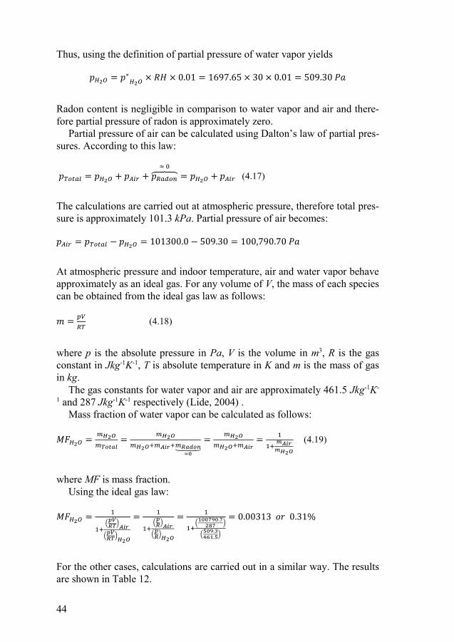
44
Thus, using the definition of partial pressure of water vapor yields
𝑝𝑝𝐻𝐻2𝑂𝑂 = 𝑝𝑝∗𝐻𝐻2𝑂𝑂 × 𝑅𝑅𝑅𝑅 × 0.01 = 1697.65 × 30 × 0.01 = 509.30 𝑃𝑃𝑃𝑃
Radon content is negligible in comparison to water vapor and air and there-fore partial pressure of radon is approximately zero.
Partial pressure of air can be calculated using Dalton’s law of partial pres-sures. According to this law:
𝑝𝑝𝑇𝑇𝑇𝑇𝑇𝑇𝑇𝑇𝑇𝑇 = 𝑝𝑝𝐻𝐻2𝑂𝑂 + 𝑝𝑝𝐴𝐴𝐴𝐴𝐴𝐴 + 𝑝𝑝𝑅𝑅𝑇𝑇𝑎𝑎𝑇𝑇𝑎𝑎⏞ ≈ 0
= 𝑝𝑝𝐻𝐻2𝑂𝑂 + 𝑝𝑝𝐴𝐴𝐴𝐴𝐴𝐴 (4.17)
The calculations are carried out at atmospheric pressure, therefore total pres-sure is approximately 101.3 kPa. Partial pressure of air becomes:
𝑝𝑝𝐴𝐴𝐴𝐴𝐴𝐴 = 𝑝𝑝𝑇𝑇𝑇𝑇𝑇𝑇𝑇𝑇𝑇𝑇 − 𝑝𝑝𝐻𝐻2𝑂𝑂 = 101300.0 − 509.30 = 100,790.70 𝑃𝑃𝑃𝑃
At atmospheric pressure and indoor temperature, air and water vapor behave approximately as an ideal gas. For any volume of V, the mass of each species can be obtained from the ideal gas law as follows:
𝑚𝑚 = 𝑝𝑝𝑝𝑝𝑅𝑅𝑇𝑇 (4.18)
where p is the absolute pressure in Pa, V is the volume in m3, R is the gas constant in Jkg-1K-1, T is absolute temperature in K and m is the mass of gas in kg.
The gas constants for water vapor and air are approximately 461.5 Jkg-1K-
1 and 287 Jkg-1K-1 respectively (Lide, 2004) . Mass fraction of water vapor can be calculated as follows:
𝑀𝑀𝑀𝑀𝐻𝐻2𝑂𝑂 =𝑚𝑚𝐻𝐻2𝑂𝑂𝑚𝑚𝑇𝑇𝑇𝑇𝑇𝑇𝑇𝑇𝑇𝑇
= 𝑚𝑚𝐻𝐻2𝑂𝑂𝑚𝑚𝐻𝐻2𝑂𝑂+𝑚𝑚𝐴𝐴𝐴𝐴𝐴𝐴+𝑚𝑚𝑅𝑅𝑇𝑇𝑅𝑅𝑇𝑇𝑅𝑅⏟
≈0
= 𝑚𝑚𝐻𝐻2𝑂𝑂𝑚𝑚𝐻𝐻2𝑂𝑂+𝑚𝑚𝐴𝐴𝐴𝐴𝐴𝐴
= 11+ 𝑚𝑚𝐴𝐴𝐴𝐴𝐴𝐴𝑚𝑚𝐻𝐻2𝑂𝑂
(4.19)
where MF is mass fraction. Using the ideal gas law:
𝑀𝑀𝑀𝑀𝐻𝐻2𝑂𝑂 =1
1+(𝑝𝑝𝑝𝑝𝑅𝑅𝑇𝑇)𝐴𝐴𝐴𝐴𝐴𝐴(𝑝𝑝𝑝𝑝𝑅𝑅𝑇𝑇)𝐻𝐻2𝑂𝑂
= 1
1+(𝑝𝑝𝑅𝑅)𝐴𝐴𝐴𝐴𝐴𝐴(𝑝𝑝𝑅𝑅)𝐻𝐻2𝑂𝑂
= 1
1+(100790.7287 )
(509.3461.5)
= 0.00313 𝑜𝑜𝑜𝑜 0.31%
For the other cases, calculations are carried out in a similar way. The results are shown in Table 12.
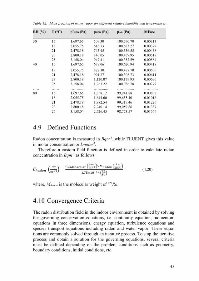
45
Table 12. Mass fraction of water vapor for different relative humidity and temperatures
RH (%) T (°C) p*H2O (Pa) pH2O (Pa) pAir (Pa) MFH2O
30 15 1,697.65 509.30 100,790.70 0.00313 18 2,055.75 616.73 100,683.27 0.00379 21 2,478.18 743.45 100,556.55 0.00458 23 2,800.18 840.05 100,459.95 0.00517 25 3,158.04 947.41 100,352.59 0.00584
40 15 1,697.65 679.06 100,620.94 0.00418 18 2,055.75 822.30 100,477.70 0.00506 21 2,478.18 991.27 100,308.73 0.00611 23 2,800.18 1,120.07 100,179.93 0.00690 25 3,158.04 1,263.22 100,036.78 0.00779 …… …… ……....... ……....... …….......... ……....... 80 15 1,697.65 1,358.12 99,941.88 0.00838
18 2,055.75 1,644.60 99,655.40 0.01016 21 2,478.18 1,982.54 99,317.46 0.01226 23 2,800.18 2,240.14 99,059.86 0.01387 25 3,158.04 2,526.43 98,773.57 0.01566
Defined Functions
Radon concentration is measured in Bqm-3, while FLUENT gives this value in molar concentration or kmolm-3.
Therefore a custom field function is defined in order to calculate radon concentration in Bqm-3 as follows:
𝐶𝐶𝑅𝑅𝑅𝑅𝑅𝑅𝑅𝑅𝑅𝑅 ( 𝐵𝐵𝐵𝐵𝑚𝑚−3) =
𝐶𝐶𝑅𝑅𝑅𝑅𝑅𝑅𝑅𝑅𝑅𝑅,𝑀𝑀𝑅𝑅𝑀𝑀𝑅𝑅𝑀𝑀 (𝑘𝑘𝑘𝑘𝑅𝑅𝑀𝑀𝑘𝑘−3 )×𝑀𝑀𝑅𝑅𝑅𝑅𝑅𝑅𝑅𝑅𝑅𝑅 ( 𝑘𝑘𝑘𝑘
𝑘𝑘𝑘𝑘𝑅𝑅𝑀𝑀)
1.75×10⁻¹⁹ (𝑘𝑘𝑘𝑘𝐵𝐵𝐵𝐵)
(4.20)
where, MRadon is the molecular weight of 222Rn.
Convergence Criteria
The radon distribution field in the indoor environment is obtained by solving the governing conservation equations, i.e. continuity equation, momentum equations in three dimensions, energy equation, turbulence equations and species transport equations including radon and water vapor. These equa-tions are commonly solved through an iterative process. To stop the iterative process and obtain a solution for the governing equations, several criteria must be defined depending on the problem conditions such as geometry, boundary conditions, initial conditions, etc.

46
In this work, six convergence criteria are considered for stopping the iter-ative process, and these must be met simultaneously. It should be noted that convergence is in principle achieved by minimizing the numerical residuals that represent the physical condition that is sought to be attained. Residuals in the order of 10-3 or better are considered as sufficient, and the respective convergence criterion represented by the residual in question is then consid-ered to have been met.
The first convergence criterion is that the radon concentration at the outlet is equal to the average radon concentration generated in the room. Second, the average static temperature must also no longer vary at the moment of convergence. Third, since the model is solved as steady-state and there is a unique outlet, at the convergence situation the radon flow rate in outlet must exactly be equal to the radon entry rate into the room, namely 0.53 Bqs-1, and it must not vary over time. Fourth, residuals must also be considered through the iterative process. Residuals are a measure of imbalances in each conser-vation equation. These must not change drastically (i.e., the rate of change of the residuals) through the iterative process, yet residuals alone cannot imply the convergence of an iterative process. Fifth, mass balance must be met in the model. Mass enters through the supply air terminal device (input mass through the radon generation in the floor can be neglected and is considered as a separate criterion) and leaves the model through the outlet. Both must be equal in the convergence situation since the model is solved in the steady state. Sixth, energy balance must also be met. In other words, since the mod-el is solved as steady-state, incoming energy flows must be equal to outgoing energy flows. Incoming energy flows include the energy which enters through the supply air terminal device (input energy through the generated radon in the floor can be neglected). Outgoing energy flows include the en-ergy which leaves the model through the outlet in addition to energy loss to the outdoor environment.
Near-wall treatment
The shear stress transport (SST) k-ω turbulence model used in this study requires meshing of the model environment.
Flow near the wall can be divided into regions designated viscous, buffer and fully turbulent sub-layers.
In the laminar (viscous) sub-layer region (y+ < 5, y+ refers to the dimen-sionless distance of the first node from the wall) inertial forces are less dom-inant and the flow exhibits laminar characteristics. This is known as the low-Re region. The SST turbulent model is a low-Re turbulent model which aims to resolve this area, and therefore requires an appropriate mesh resolution to do this accurately. In the log law (fully turbulent) region, convective forces

47
dominate over viscous forces and create high turbulent stresses; this is known as the high-Re composite region. In the SST turbulent model the entire turbulent boundary layer is resolved, including the log law region. However, it is possible to use semi-empirical expressions known as wall functions to bridge the viscosity-affected region between the wall and the fully turbulent region.
When using low-Re models such as the SST turbulent model, the average y+ value (the first node dimensionless distance from the wall) should be in the order of ~1 to ensure that the laminar sub-layer is being captured (Gerasimov, 2006). High quality numerical results for the boundary layer will only be obtained if the overall resolution of the boundary layer is suffi-cient. The minimum number of cells to cover a boundary layer accurately is around 10, but values of 20 are desirable. The total thickness should be im-plemented such that around 15 or more nodes cover the boundary layer (ANSYS Inc, 2011).
Going by the above, since in this study the SST turbulent model is used, y+=1 is chosen for calculation of the distance of the first node from the wall, and the resolution of the boundary layer is set to 12 with a specific growth factor between the nodes to accurately capture the boundary layer.
Calculations to obtain the first node distance from the wall and the ratio between the cells (growth factor) are shown below for Ach = 0.5 hr1.
Wall shear stress, according to the definition, can be calculated from the following expression:
𝜏𝜏𝑊𝑊 = 12 𝐶𝐶𝑓𝑓𝜌𝜌𝑉𝑉𝑉𝑉𝑉𝑉𝑉𝑉𝑉𝑉
2 (4.21)
where, Cf is the skin friction, VVent is the flow velocity at the supply air ter-minal device and ρ is the density of air. Cf is obtained from the following approximation formula:
𝐶𝐶𝑓𝑓 = [2𝐿𝐿𝐿𝐿𝐿𝐿10(𝑅𝑅𝑅𝑅𝑅𝑅𝑅𝑅𝑅𝑅𝑅𝑅) − 0.65]−2.3 𝑓𝑓𝐿𝐿𝑓𝑓 𝑅𝑅𝑅𝑅𝑅𝑅𝑅𝑅𝑅𝑅𝑅𝑅 < 109
In this case (Ach=0.5 hr-1), thus
𝐶𝐶𝑓𝑓 = [2𝐿𝐿𝐿𝐿𝐿𝐿10(2692.7) − 0.65]−2.3 = 0.015
𝜏𝜏𝑊𝑊 = 12 × 0.015 × 1.225 × (0.164)2 = 2.47 × 10⁻⁴ 𝑘𝑘𝑘𝑘
𝑅𝑅𝑠𝑠2
According to the definition, first node distance (𝑦𝑦) from the wall can be obtained from the following expression:

48
𝑦𝑦 = 𝑦𝑦+𝜇𝜇𝜌𝜌𝑢𝑢𝜏𝜏
(4.22)
where ρ and μ are the density and the dynamic viscosity of air respectively and 𝑢𝑢𝜏𝜏 is the friction velocity. Dimensional analysis shows that friction ve-locity (which is a characteristic velocity at the wall) can be defined in the following way:
𝑢𝑢𝜏𝜏 = √𝜏𝜏𝑊𝑊𝜌𝜌 (4.23)
where ρ is the density of air and 𝜏𝜏𝑊𝑊 is wall shear stress. In this case (Ach=0.5 hr-1), and thus for 𝑦𝑦+ = 𝑢𝑢+ =1 this gives:
𝑢𝑢𝜏𝜏 = √2.466 × 10⁻⁴
1.225 = 0.014 𝑚𝑚𝑠𝑠
The first node distance (𝑦𝑦) can be calculated from Equation 4.22 as follows:
𝑦𝑦 = 1 × 1.7894 × 10−5
1.225 × 0.014 = 1.04 𝑚𝑚𝑚𝑚
12 cells in the boundary layer with a specific ratio between the cells are used in order to accurately capture the boundary layer. In order to determine this ratio, the boundary layer thickness must be provided. At the boundary layer edge, the velocity is equal to the free stream velocity. Dimensionless veloci-ty for a wall-bounded flow is defined as follows:
𝑢𝑢+ = 𝑉𝑉𝑢𝑢𝜏𝜏
(4.24)
where 𝑉𝑉 is the local velocity and 𝑢𝑢𝜏𝜏 is the friction velocity. According to the law of the wall, u+ and y+ are correlated in the log-layer
region as follows:
𝑢𝑢+ = 10.41 𝐿𝐿𝐿𝐿(𝑦𝑦+) + 5.1 (4.25)
And in the laminar sub-layer region (y+<15):
𝑢𝑢+ = 𝑦𝑦+

49
In this case (Ach=0.5 hr-1) the maximum u+ (at the boundary layer edge) can be calculated as follows:
𝑢𝑢𝐸𝐸𝐸𝐸𝐸𝐸𝐸𝐸+ = 𝑉𝑉𝑉𝑉𝐸𝐸𝑉𝑉𝑉𝑉
𝑢𝑢𝑉𝑉=
0.164 𝑚𝑚𝑠𝑠
0.014 𝑚𝑚𝑠𝑠
= 11.7
By using the law of the wall in the log-layer region (see Equation 4.25), the corresponding y+ for the above u+ can be calculated as the following:
𝑦𝑦𝐸𝐸𝐸𝐸𝐸𝐸𝐸𝐸+ = 𝑒𝑒(0.41𝑢𝑢+−5.1) = 𝑒𝑒(0.41×11.55−5.1) = 14.08
and therefore boundary layer thickness, which is the corresponding 𝑦𝑦 for the 𝑦𝑦𝐸𝐸𝐸𝐸𝐸𝐸𝐸𝐸
+ , can be calculated as follows:
𝛿𝛿 ≡ 𝑦𝑦𝐸𝐸𝐸𝐸𝐸𝐸𝐸𝐸 =𝑦𝑦𝐸𝐸𝐸𝐸𝐸𝐸𝐸𝐸
+ 𝜇𝜇𝜌𝜌𝑢𝑢𝑉𝑉
= 14.08 × 1.7894 × 10−5
1.225 × 0.014 = 14.7 𝑚𝑚𝑚𝑚
where δ is the boundary layer thickness. The nodes are placed within the boundary layer with a specific growth
factor. Therefore, boundary layer thickness can also be obtained from the following expression as the sum of the geometric series of cells sizes within the boundary layer:
𝛿𝛿 = 𝑦𝑦(𝑟𝑟𝑛𝑛−1)𝑟𝑟−1 (4.26)
where y is the first node distance from the wall, r is the ratio between the cells (growth factor) and n is the number of cells within the boundary layer.
For the calculated values of y and δ for this case (Ach = 0.5 hr-1) and con-sidering 12 cells within the boundary layer (n=12), 𝑟𝑟 = 1.03. For other venti-lation rates, calculations can be carried out in a similar way.
A sample of the meshed model from the isometric view is shown in Fig-ure 7. In the figure, boundary layer cells can be easily seen.
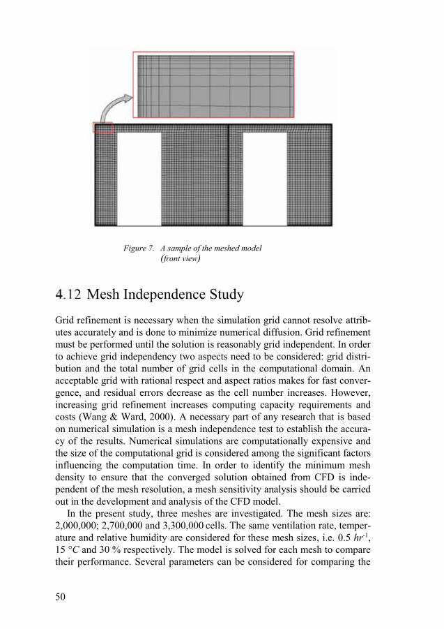
50
Figure 7. A sample of the meshed model (front view)
Mesh Independence Study
Grid refinement is necessary when the simulation grid cannot resolve attrib-utes accurately and is done to minimize numerical diffusion. Grid refinement must be performed until the solution is reasonably grid independent. In order to achieve grid independency two aspects need to be considered: grid distri-bution and the total number of grid cells in the computational domain. An acceptable grid with rational respect and aspect ratios makes for fast conver-gence, and residual errors decrease as the cell number increases. However, increasing grid refinement increases computing capacity requirements and costs (Wang & Ward, 2000). A necessary part of any research that is based on numerical simulation is a mesh independence test to establish the accura-cy of the results. Numerical simulations are computationally expensive and the size of the computational grid is considered among the significant factors influencing the computation time. In order to identify the minimum mesh density to ensure that the converged solution obtained from CFD is inde-pendent of the mesh resolution, a mesh sensitivity analysis should be carried out in the development and analysis of the CFD model.
In the present study, three meshes are investigated. The mesh sizes are: 2,000,000; 2,700,000 and 3,300,000 cells. The same ventilation rate, temper-ature and relative humidity are considered for these mesh sizes, i.e. 0.5 hr-1, 15 °C and 30 % respectively. The model is solved for each mesh to compare their performance. Several parameters can be considered for comparing the

51
performance of different mesh sizes. In this work, four parameters are con-sidered for this purpose, average radon concentration, average static temper-ature, radon flow rate in the outlet and radon concentration along a vertical line in the middle of the room.
The results after convergence for each mesh for the first three parameters are presented in Table 13. Table 13. Average radon concentration, average static temperature and radon flow rate in
the outlet for different mesh sizes
Mesh size (Cells)
Average radon concentration Radon flow rate in the outlet
C Radon (Bqm-3)
Error (%) ṁ Radon (Bqs-1)
Error (%)
2,000,000 37.004 - 0.5473 - 2,700,000 37.124 0.33 0.5766 3.40 3,300,000 37.188 0.17 0.5842 1.30
Percentage errors in each row in Table 13 have been calculated relative to the preceding row. Therefore, the first row does not have a percentage error.
Table 13 clearly shows that between the results of 2,000,000 cells and 2,700,000 cells there is a jump in the values of interest, especially in the average radon concentration, which is very important to this work. However, between the results of 2,700,000 cells and 3,300,000 cells, differences are negligible, especially the difference between the values of average radon concentration, which is less than 0.2%.
For better visualization, average radon concentration, average static tem-perature and radon flow rate in the outlet for different meshes sizes have been plotted in Figures 8 to 10. These figures clearly show that the differ-ences between the results from 2,700,000 cells and 3,300,000 cells are negli-gible, and that there is a larger difference between the results with 2,000,000 cells and other mesh densities, especially in average radon concentration.

52
Figure 8. Average radon concentration for different mesh sizes
Figure 9. Average static temperature for different mesh sizes
36
38
40
42
44
800,000 1,300,000 1,800,000 2,300,000 2,800,000 3,300,000
Rad
on le
vel (
Bq/
m3)
Number of cells
272
272.2
272.4
272.6
272.8
273
800,000 1,300,000 1,800,000 2,300,000 2,800,000 3,300,000
T (K
)
Number of cells

53
Figure 10. Radon flow rate in the outlet for different mesh sizes
The fourth parameter which is considered in this study for comparing per-formance of different mesh sizes is the radon concentration profile along a vertical line in the middle of the room. Figure 11 shows this parameter for the different mesh sizes.
Figure 11. Radon concentration profile along a vertical line in the middle of the room for different mesh sizes
Figure 11 shows that the radon concentration profile also has the same shape for all the different mesh densities tested. It is evident that as the number of
0.8
0.82
0.84
0.86
0.88
0.9
800000 1300000 1800000 2300000 2800000 3300000
Rad
on fl
ow ra
te in
out
let (
Bq/
s)
Number of cells

54
cells in the mesh is increased, the variation in the radon concentration profile decreases. Thus the change in radon concentration profile between meshes with 2,700,000 and 3,300,000 cells is negligible.
Based on the above, we can be confident that a mesh with 2,700,000 cells is sufficient to carry out the simulations, as it gives a mesh-independent re-sult at the minimum possible computational cost. Therefore this number of cells is selected for the simulations in this study.
Examination of convergence criteria
Simulations were carried out for the different cases indicated in Table 9. Within each simulation, all convergence criteria must be met to obtain a solution for the case. In this section, convergence criteria are examined for the case designated N11 in Table 9 (Ach = 1.0 hr-1, T = 23 °C, RH = 40%). A similar procedure is used for the other cases.
As mentioned before, six convergence criteria are considered for deter-mining the convergence of the iterative process to obtain a solution.
The first convergence criterion is the average radon concentration in the room. At convergence, average radon concentration must no longer change. Figure 12 shows plot average radon concentration against iterations, show-ing that average radon concentration approaches a specific value after which it does not change with increasing iterations. The first convergence criterion is therefore satisfied.
Figure 12. Average radon concentration versus iterations for the case N11
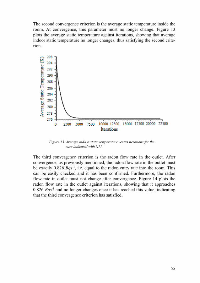
55
The second convergence criterion is the average static temperature inside the room. At convergence, this parameter must no longer change. Figure 13 plots the average static temperature against iterations, showing that average indoor static temperature no longer changes, thus satisfying the second crite-rion.
Figure 13. Average indoor static temperature versus iterations for the case indicated with N11
The third convergence criterion is the radon flow rate in the outlet. After convergence, as previously mentioned, the radon flow rate in the outlet must be exactly 0.826 Bqs-1, i.e. equal to the radon entry rate into the room. This can be easily checked and it has been confirmed. Furthermore, the radon flow rate in outlet must not change after convergence. Figure 14 plots the radon flow rate in the outlet against iterations, showing that it approaches 0.826 Bqs-1 and no longer changes once it has reached this value, indicating that the third convergence criterion has satisfied.

56
Figure 14. Radon flow rate in the outlet versus iterations for the case indicated with N11
The fourth convergence criterion concerns the residuals. Figure 15 plots the residuals versus iterations. The residuals do not change drastically and their variations are moderate with increasing iterations. Therefore, the fourth con-vergence criterion has also been satisfied.

57
Figure 15. Residuals versus iterations for the case indicated with N11
The fifth convergence criterion is the mass balance. In order to calculate the mass balance, the input mass flow rate at the vent is first calculated as fol-lows. Input flow contains three species; radon, water vapor and air. Mass fraction of radon at the vent is zero. Mass fraction of water vapor for case N11 is obtained from Table 12, and from this the mass fraction of air can be determined.
𝑀𝑀𝑀𝑀𝐻𝐻2𝑂𝑂 = 0.0069
Mass flow rate can be calculated from the following equation:
��𝑚 = 𝜌𝜌𝑉𝑉𝑉𝑉𝑉𝑉𝑉𝑉𝑉𝑉𝐴𝐴𝑉𝑉𝑉𝑉𝑉𝑉𝑉𝑉
where AVent is the area of the vent which is 0.06 m2. VVent is the velocity at the vent, and according to Table 7 for case N11 it is 0.328 ms-1. ρ is the density of the mixture, which can be calculated from the ideal gas law as follows:
𝑃𝑃𝑉𝑉 = 𝑚𝑚𝑀𝑀𝑀𝑀𝑀𝑀𝑀𝑀𝑀𝑀𝑀𝑀𝑀𝑀𝑀𝑀
��𝑅𝑇𝑇 (4.27)

58
where m is the mass of the mixture and MMixture is the molar mass of the mix-ture. P is the absolute pressure (101,300.0 Pa), V is the volume of the mix-ture, n is the number of moles in the mixture and the universal gas constant ��𝑅 is 8.31446 Jmol-1K-1 (Lide, 2004). T is the absolute temperature, in this case (N11) it is 23 + 273 = 296 K.
Density of the mixture 𝜌𝜌 = 𝑚𝑚𝑉𝑉 , which using the ideal gas law, gives
𝜌𝜌 = 𝑃𝑃𝑀𝑀𝑀𝑀𝑀𝑀𝑀𝑀𝑀𝑀𝑀𝑀𝑀𝑀𝑀𝑀��𝑅𝑇𝑇
Therefore, for the density of mixture calculation, the molar mass of the mix-ture should be calculated. The molar mass of the mixture is calculated as follows:
𝑀𝑀𝑀𝑀𝑀𝑀𝑀𝑀𝑀𝑀𝑀𝑀𝑀𝑀𝑀𝑀 =𝑚𝑚
𝑛𝑛𝑇𝑇𝑇𝑇𝑀𝑀𝑇𝑇𝑇𝑇 (4.28)
where m is the total mass of the mixture and nTotal is the total number of moles within the mixture.
As mentioned before, there is no radon at the inlet (vent). Therefore, the total number of moles at the inlet only includes the number of moles of wa-ter vapor and air.
𝑀𝑀𝑀𝑀𝑀𝑀𝑀𝑀𝑀𝑀𝑀𝑀𝑀𝑀𝑀𝑀 =𝑚𝑚
𝑛𝑛𝐻𝐻2𝑂𝑂+𝑛𝑛𝐴𝐴𝑀𝑀𝑀𝑀
Number of moles of water vapor and air can be calculated as follows:
𝑛𝑛𝐻𝐻2𝑂𝑂 =𝑚𝑚𝐻𝐻2𝑂𝑂𝑀𝑀𝐻𝐻2𝑂𝑂
𝑛𝑛𝐴𝐴𝑀𝑀𝑀𝑀 =𝑚𝑚𝐴𝐴𝑀𝑀𝑀𝑀𝑀𝑀𝐴𝐴𝑀𝑀𝑀𝑀
where 𝑀𝑀𝐻𝐻2𝑂𝑂 and 𝑀𝑀𝐴𝐴𝑀𝑀𝑀𝑀 are the molar mass of water vapor and air respective-ly. Using the mass fraction of water vapor, gives
𝑛𝑛𝐻𝐻2𝑂𝑂 =𝑚𝑚𝐻𝐻2𝑂𝑂𝑀𝑀𝐻𝐻2𝑂𝑂
= 𝑚𝑚×𝑀𝑀𝑀𝑀𝐻𝐻2𝑂𝑂𝑀𝑀𝐻𝐻2𝑂𝑂
Since the mass fraction of radon at the supply air terminal device (vent) is zero, the mass fraction of air can be obtained from the following expression:
𝑀𝑀𝑀𝑀𝐴𝐴𝑀𝑀𝑀𝑀 = 1 − 𝑀𝑀𝑀𝑀𝐻𝐻2𝑂𝑂

59
Therefore, the number of moles of air is:
𝑛𝑛𝐴𝐴𝐴𝐴𝐴𝐴 = 𝑚𝑚𝐴𝐴𝐴𝐴𝐴𝐴𝑀𝑀𝐴𝐴𝐴𝐴𝐴𝐴
= 𝑚𝑚×𝑀𝑀𝑀𝑀𝐴𝐴𝐴𝐴𝐴𝐴𝑀𝑀𝐴𝐴𝐴𝐴𝐴𝐴
= 𝑚𝑚×(1−𝑀𝑀𝑀𝑀𝐻𝐻2𝑂𝑂)𝑀𝑀𝐴𝐴𝐴𝐴𝐴𝐴
Substituting the expressions for the number of moles of water vapor and air in the molar mass expression for the mixture gives
𝑀𝑀𝑀𝑀𝐴𝐴𝑀𝑀𝑀𝑀𝑀𝑀𝐴𝐴𝑀𝑀 = 𝑚𝑚𝑛𝑛𝐻𝐻2𝑂𝑂+𝑛𝑛𝐴𝐴𝐴𝐴𝐴𝐴
= 𝑚𝑚𝑚𝑚×𝑀𝑀𝑀𝑀𝐻𝐻2𝑂𝑂
𝑀𝑀𝐻𝐻2𝑂𝑂+
𝑚𝑚×(1−𝑀𝑀𝑀𝑀𝐻𝐻2𝑂𝑂)𝑀𝑀𝐴𝐴𝐴𝐴𝐴𝐴
= 1𝑀𝑀𝑀𝑀𝐻𝐻2𝑂𝑂𝑀𝑀𝐻𝐻2𝑂𝑂
+(1−𝑀𝑀𝑀𝑀𝐻𝐻2𝑂𝑂)
𝑀𝑀𝐴𝐴𝐴𝐴𝐴𝐴
Using the value of 𝑀𝑀𝑀𝑀𝐻𝐻2𝑂𝑂 for case N11 and the data in Table 9, the molar mass of the mixture can be calculated as follows:
𝑀𝑀𝑀𝑀𝐴𝐴𝑀𝑀𝑀𝑀𝑀𝑀𝐴𝐴𝑀𝑀 = 1𝑀𝑀𝑀𝑀𝐻𝐻2𝑂𝑂𝑀𝑀𝐻𝐻2𝑂𝑂
+(1−𝑀𝑀𝑀𝑀𝐻𝐻2𝑂𝑂)
𝑀𝑀𝐴𝐴𝐴𝐴𝐴𝐴
= 10.0069
18.015 ( 𝑘𝑘𝑘𝑘𝑘𝑘𝑚𝑚𝑘𝑘𝑘𝑘)
+ (1−0.0069)28.966 ( 𝑘𝑘𝑘𝑘
𝑘𝑘𝑚𝑚𝑘𝑘𝑘𝑘)
= 28.845 𝑘𝑘𝑘𝑘𝑘𝑘𝑚𝑚𝑘𝑘𝑘𝑘
Therefore, density of the mixture can be calculated as follows:
𝜌𝜌 = 𝑃𝑃𝑀𝑀𝑀𝑀𝐴𝐴𝑀𝑀𝑀𝑀𝑀𝑀𝐴𝐴𝑀𝑀��𝑅𝑇𝑇 = 101300.0 𝑃𝑃𝑃𝑃×28.845 𝑘𝑘𝑘𝑘
𝑘𝑘𝑚𝑚𝑘𝑘𝑘𝑘× 1 𝑘𝑘𝑚𝑚𝑘𝑘𝑘𝑘1000 𝑚𝑚𝑘𝑘𝑘𝑘
8.31446 𝐽𝐽𝑚𝑚𝑘𝑘𝑘𝑘𝑚𝑚×296 𝐾𝐾
= 1.187 𝑘𝑘𝑘𝑘𝑚𝑚3
and the mass flow rate at the supply air terminal device (input mass) is:
��𝑚 = 𝜌𝜌𝑉𝑉𝑉𝑉𝑀𝑀𝑛𝑛𝑀𝑀𝐴𝐴𝑉𝑉𝑀𝑀𝑛𝑛𝑀𝑀 = 1.187 𝑘𝑘𝑘𝑘𝑚𝑚3 × 0.328 𝑚𝑚
𝑠𝑠 × 0.06 𝑚𝑚2 = 0.023 𝑘𝑘𝑘𝑘𝑠𝑠
In order to verify the mass balance we must also examine the mass flow rate at the outlet. There is only one outlet in the model. FLUENT gives a value of 0.023 (kgs-1) for the radon flow rate at the outlet. Therefore the mass balance is met and thus the fifth convergence criterion has also been satisfied.
The sixth convergence criterion is the energy balance. Input energies in-clude the input energy through the vent and the input energy from radon. The radon flow rate through the floor is negligible in comparison with the flow rate at the supply air terminal device. The input energy from radon can therefore be ignored. There is thus only one source of input energy, namely the supply air terminal device (inlet). Output energies include the output energy through the outlet and heat rejection to the outdoor environment through the outer surfaces (including outside walls, roof, window and main door). First, the difference between the input energy through the supply air terminal device and the output energy through the outlet is calculated. The

60
obtained value must be equal to the heat rejection to the outdoor environ-ment through the outer surfaces to achieve energy balance.
The difference between the input energy through the supply air terminal device and the output energy through the outlet can be calculated as fol-lows3:
𝑄𝑄1 = 𝑄𝑄𝐴𝐴𝐴𝐴𝐴𝐴 + 𝑄𝑄𝑊𝑊𝑊𝑊𝑊𝑊𝑊𝑊𝐴𝐴 = ��𝑚𝐴𝐴𝐴𝐴𝐴𝐴𝑐𝑐𝑝𝑝,𝐴𝐴𝐴𝐴𝐴𝐴(𝑇𝑇𝑉𝑉𝑊𝑊𝑉𝑉𝑊𝑊 − 𝑇𝑇𝑂𝑂𝑂𝑂𝑊𝑊𝑂𝑂𝑊𝑊𝑊𝑊) + ��𝑚𝐻𝐻2𝑂𝑂𝑐𝑐𝑝𝑝,𝐻𝐻2𝑂𝑂(𝑇𝑇𝑉𝑉𝑊𝑊𝑉𝑉𝑊𝑊 − 𝑇𝑇𝑂𝑂𝑂𝑂𝑊𝑊𝑂𝑂𝑊𝑊𝑊𝑊)
where Q1 is the difference between the input energy through the supply air terminal device and the output energy through the outlet, ��𝑚𝐴𝐴𝐴𝐴𝐴𝐴 and ��𝑚𝐻𝐻2𝑂𝑂 are the mass flow rate of air and water vapor respectively in the model, 𝑐𝑐𝑝𝑝,𝐴𝐴𝐴𝐴𝐴𝐴 and 𝑐𝑐𝑝𝑝,𝐻𝐻2𝑂𝑂 are the heat capacity of air and water vapor respectively and can be obtained from Table 11, TVent and TOutlet are the average static temperature of the mixture at the supply air terminal device and at the outlet respectively. TVent in the case under consideration (N11) is 23 °C and TOutlet is obtained using FLUENT, and is 1.357 °C.
Using the mass fraction of water vapor, the above equation can be rewrit-ten as follows:
𝑄𝑄1 = [��𝑚(1 − 𝑀𝑀𝑀𝑀𝐻𝐻2𝑂𝑂)𝑐𝑐𝑝𝑝,𝐴𝐴𝐴𝐴𝐴𝐴 + ��𝑚𝑀𝑀𝑀𝑀𝐻𝐻2𝑂𝑂𝑐𝑐𝑝𝑝,𝐻𝐻2𝑂𝑂](𝑇𝑇𝑉𝑉𝑊𝑊𝑉𝑉𝑊𝑊 − 𝑇𝑇𝑂𝑂𝑂𝑂𝑊𝑊𝑂𝑂𝑊𝑊𝑊𝑊) or
𝑄𝑄1 = ��𝑚(𝑇𝑇𝑉𝑉𝑊𝑊𝑉𝑉𝑊𝑊 − 𝑇𝑇𝑂𝑂𝑂𝑂𝑊𝑊𝑂𝑂𝑊𝑊𝑊𝑊)[(1 − 𝑀𝑀𝑀𝑀𝐻𝐻2𝑂𝑂)𝑐𝑐𝑝𝑝,𝐴𝐴𝐴𝐴𝐴𝐴 + 𝑀𝑀𝑀𝑀𝐻𝐻2𝑂𝑂𝑐𝑐𝑝𝑝,𝐻𝐻2𝑂𝑂]
where ��𝑚 is the total mass flow rate in the model and 𝑀𝑀𝑀𝑀𝐻𝐻2𝑂𝑂 is the mass frac-tion of water vapor.
For case N11, Q1 is
𝑄𝑄1 = 0.023(23 − 1.357)[(1 − 0.007)1006.43 + 0.007 × 2014.0] = 504.50 𝐽𝐽
The heat rejection to the outdoor environment through each outer surface is obtained from FLUENT and presented in Table 14.
Table 14. The heat rejection to outdoor environment through each outer surface, case N11
Outer surface Heat rejection (J) Outside walls 125.99 Roof 302.30 Main door 18.65 Window 58.60
3 There is no internal source in Room 1.

61
From the data in Table 14, the total heat rejection to outdoor environment, Q2, can be calculated as follows:
𝑄𝑄2 = 125.99 + 302.30 + 18.65 + 58.6 = 505.54 𝐽𝐽
Comparison between Q1 and Q2 implies that the sixth convergence criterion has been satisfied.
Thus all convergence criteria for the considered case (N11) have been sat-isfied, implying that the model has been converged and the solution has been obtained.

62

63
5 Results and discussion
Results and discussion are presented as the following: radon measurements, energy dynamics simulation and economic analysis, and numerical simula-tion.
Radon measurement
As previously mentioned, radon concentrations were measured through ATDs and CRMs. Radon levels are measured by ATD which are sent to a nuclear laboratory for processing. Data measured by the continuous radon meter are directly accessible by a computer.
Measurements of the indoor radon content in this one-family house were recorded between 2008 and 2010. During this period the building had an exhaust air ventilation system. In 2010 a heat recovery ventilation system was installed alongside some remediation actions such as floor sealing and creation of a radon sump. These actions significantly improved IAQ and reduced the indoor radon level. Indoor radon concentration in this house at the normal ventilation rate, 0.5 Ach, is currently below 100 Bqm-3. Air leak-age is not included in the air change rate in these measurements. Table 15 shows the results of indoor radon measurements in the case study house.
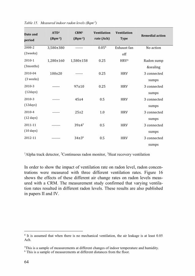
64
Table 15. Measured indoor radon levels (Bqm-3)
Date and
period
ATD1 (Bqm-3)
CRM2 (Bqm-3)
Ventilation
rate (Ach) Ventilation
Type Remedial action
2008-2 (2weeks)
3,580±380 ------ 0.054 Exhaust fan off
No action
2010-1 (3months)
1,280±160 1,580±158 0.25 HRV3 Radon sump &sealing
2010-04 (3 weeks)
100±20 ------ 0.25 HRV 3 connected sumps
2010-3 (12days)
------ 97±10 0.25 HRV 3 connected sumps
2010-3 (12days)
------ 45±4 0.5 HRV 3 connected sumps
2010-4 (12 days)
------ 25±2 1.0 HRV 3 connected sumps
2011-11 (10 days)
------- 39±45 0.5 HRV 3 connected sumps
2012-11 ------- 34±36 0.5 HRV 3 connected sumps
1Alpha track detector, 2Continuous radon monitor, 3Heat recovery ventilation
In order to show the impact of ventilation rate on radon level, radon concen-trations were measured with three different ventilation rates. Figure 16 shows the effects of these different air change rates on radon levels meas-ured with a CRM. The measurement study confirmed that varying ventila-tion rates resulted in different radon levels. These results are also published in papers II and IV.
4 It is assumed that when there is no mechanical ventilation, the air leakage is at least 0.05 Ach. 5This is a sample of measurements at different changes of indoor temperature and humidity. 6 This is a sample of measurements at different distances from the floor.

65
Figure 16. Radon level measurements versus ventilation rate
In order to show the influence of indoor temperature and relative humidity on indoor radon level, several measurements were carried out. Continuous radon measuring results do not show strong correlations between indoor radon levels and indoor RH and temperature in the tested ranges.
Figure 17 shows a sample result from the R2 CRM. Radon and tempera-ture were monitored simultaneously. Green and purple curves show fluctua-tions of radon and temperature levels in the case study house respectively. These curves indicate instantaneous changes of indoor radon and tempera-ture.
In the case of temperature it was observed that indoor radon fluctuations correlate with indoor temperature (see Figure 17). Since indoor radon level is dependent on many factors such as outdoor conditions, this relation is not strong. One possible physical interpretation could be that a higher indoor temperature increases the influence of thermals (stack effect), given its ten-dency to increase the magnitude of the negative indoor pressure at floor lev-el. This increased negative pressure would increase the infiltration of air, including radon gas, from the ground (advection effect), and for this reason we would expect to see a correlation between higher indoor temperature and higher radon content. However, this relation should be relatively weak, un-less the indoor temperature is varied more dramatically.

66
Figure 17. Radon level (green curve) and temperature (purple curve). Radon is on the red axis (Bq/m3), temperature is on the green axis, and the horizontal axis represents time in hours from 21-24 December.
Several measurements were carried out to investigate the relationship be-tween indoor radon level and the height above the floor. To measure radon level, a R2 CRM device was placed at different heights (0, 50, 90 and 200 cm) from the floor at 0.5 Ach. Figure 18 shows this relationship between the average radon level and height, which reflects the theoretical relation Equa-tion 3.3.
Figure 18. Radon level changes versus measurement height above the room floor
The horizontal axis indicates the measurement time periods for the different height set ups. The results indicate an inverse relationship between radon level and height (H).

67
To further verify the relation between indoor radon level and height above
the floor several measurements were taken at different locations. These measurements, shown in Figures 19 and 20 supported the relationship be-tween radon level and height above the floor.
Figure 19. Average radon levels versus height (0-200 cm from the floor)
Figure 20. Average radon levels versus height (0-50 cm from the floor)
28
36
44
52
60
68
76
0.04 0.34 0.64 0.94 1.24 1.54 1.84 2.14
Rad
on le
vel (
Bq/
m3)
Distance from the floor (m)
28
36
44
52
60
68
76
0.04 0.09 0.14 0.19 0.24 0.29 0.34 0.39 0.44 0.49 0.54
Rad
on le
vel (
Bq/m
3)
Distance from the floor (m)

68
Analytical analysis of radon level in the case study house
Analytic calculations from Equations (3.3) and (3.5) give indoor radon levels for different ventilation rates (0.0 to 1.0 Ach) and 𝐸𝐸 = 0.018 𝐵𝐵𝐵𝐵𝑚𝑚−2𝑠𝑠−1. The calculation results are as follows: 𝐶𝐶0.0 = 3,582 , 𝐶𝐶0.25 = 108, 𝐶𝐶0.5 = 54, and 𝐶𝐶1 = 22 Bq𝑚𝑚−3.
These results from analytic calculations were compared with the measured data listed in Table 15. The comparison is shown in Table 16.
Table 16. Radon level versus ventilation rate by measurement and analytic methods
Air change rate (Ach)
Measurement(𝐁𝐁𝐁𝐁𝒎𝒎−𝟑𝟑) Analytic(𝐁𝐁𝐁𝐁𝒎𝒎−𝟑𝟑)
≅0.0 3,580±380 3,582 0.25 97±10 108 0.5 45±4 54 1.0 25±2 22
The comparison in Table 16 shows that indoor radon levels resulting from analytical calculations corresponded closely with the measured data, with a maximum difference of 14%.
Dynamic energy simulation and calculation
The annual recoverable energy with constant room temperature can be easily determined by energy calculation and dynamic energy with IDA ICE. The annual energy saving is generally varied by changing the ventilation rate and heating degree days (HDD). Several dynamic simulations were carried out for different ventilation rates and heat exchanger unit efficiencies. IDA ICE uses its own database to estimate HDD. The Stockholm, Bromma climate profile in the database was selected for this study. The energy data is based on available data for the heat exchanger unit produced by the FLEXIT Com-pany, and the energy calculation for the case study house is based on Equa-tion 3.11. The results of the dynamic simulation are shown in Table 17.

69
Table 17. Dynamic simulation and energy calculation results
Ventilation rate (Ach)
Heat recovery (kWh) simulation
Heat recovery (kWh) calculation
0.5 3,380 3,200
1.0 6,759 6,400
Comparison of these simulation and calculation results shows good agree-ment between the data with an error of about 6 % at 0.5 Ach. This discrep-ancy results from the different values of the heat recovery unit efficiency and heating degree days used in these methods.
The normal range of the ventilation rate and HDD in similar cold climates is typically 0.5–1 Ach and 4,000–6,000 degree days respectively. The annual heat recovery through this type of ventilation system would be in the range of 20 to 90 kWh per 𝑚𝑚2 per floor area. For this case study the annual heat recovery is about 30 kWh per 𝑚𝑚2 per floor area.
5.3.1 Economic analysis of the heat recovery ventilation unit The net present value (NPV) method was used to evaluate the cost-effectiveness of a future investment as discussed in Paper I.
The initial capital investment and installation cost of the rotary heat ex-changer unit is about 25,000 SEK, with 25 years lifetime. The energy con-sumption of the 2 DC fans is 350 kWh per year and the cost of replacing the 2 filters is 500 SEK per year. Energy costs in Sweden are roughly 1 SEK/kWh including tax and VAT. It should be noted that the 25,000 SEK only covers the heat exchanger unit itself. If the assessment included instal-lation of an exhaust air ventilation system with a supply air and exhaust air system, the total (higher) cost for the supply air system with ducting etc. should be included. In this case the assumption is that the supply air system is already in place, and thus only the additional investment for the heat ex-changer unit is considered.
A comparison against all possible exhaust air ventilation systems has been deemed to lie outside the scope of this thesis. It is worth mentioning that exhaust air heat pumps are very commonly used in Swedish one-family houses. The economic study in this thesis does not include any comparison with heat pumps. This choice is not expected to affect the overall conclu-sions drawn from the research.
NPV can be calculated based on Equations 3.14–3.17. Annual savings: b = Costs of recovered energy per year - Annual mainte-
nance cost (3,168-350-500 = 2,318 SEK), and therefore B0= 36,207 SEK and A0 = 25,000 SEK, which means that B0 > A0. Table 18 shows the details of these values.
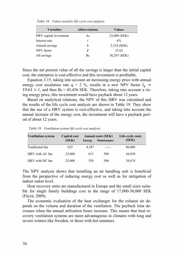
70
Table 18. Values used for life cycle cost analysis
Variables Abbreviations Values
HRV capital investment A0 25,000 (SEK) Interest rate 𝑖𝑖 4% Annual savings b 2,318 (SEK) NPV factor 𝑰𝑰 15.62 All savings B0 36,207 (SEK)
Since the net present value of all the savings is larger than the initial capital cost, the enterprise is cost-effective and this investment is profitable.
Equation 3.15, taking into account an increasing energy price with annual energy cost escalation rate q = 2 %, results in a new NPV factor 𝐼𝐼𝑞𝑞 =19.61 > 𝐼𝐼, and then B0 = 45,456 SEK. Therefore, taking into account a ris-ing energy price, this investment would have payback about 12 years.
Based on analytical relations, the NPV of this HRV was calculated and the results of the life cycle cost analysis are shown in Table 19. They show that the use of a HRV system is cost-effective, and taking into account the annual increase of the energy cost, the investment will have a payback peri-od of about 12 years.
Table 19. Ventilation system life cycle cost analysis
Ventilation system Capital cost (SEK)
Annual costs (SEK) Energy Maintenance
Life-cycle costs (SEK)
Traditional fan 625 4,387 ----- 86,000
HRV with AC fan 25,000 613 500 44,830
HRV with DC fan 25,000 350 500 39,674
The NPV analysis shows that installing an air handling unit is beneficial from the perspective of reducing energy cost as well as for mitigation of indoor radon level.
Heat recovery units are manufactured in Europe and the small sizes suita-ble for single family buildings cost in the range of 17,000-30,000 SEK (Flexit, 2009).
The economic evaluation of the heat exchanger for the exhaust air de-pends on the volume and duration of the ventilation. The payback time de-creases when the annual utilization hours increase. This means that heat re-covery ventilation systems are more advantageous in climates with long and severe winters like Sweden, or those with hot summers.
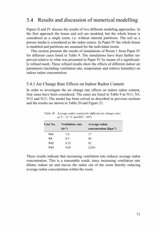
71
Results and discussion of numerical modelling
Papers II and IV discuss the results of two different modeling approaches. In the first approach the house and soil are modeled, but the whole house is considered as a single room, i.e. without internal partitions. The soil as a porous media is considered as the radon source. In Paper IV the whole house is modeled and partitions are assumed for the individual rooms
This section presents the results of simulations of Room 1 from Paper IV for different cases listed in Table 9. The simulations have been further im-proved relative to what was presented in Paper IV by means of a significant-ly refined mesh. These refined results show the effects of different indoor air parameters (including ventilation rate, temperature and relative humidity) on indoor radon concentration.
5.4.1 Air Change Rate Effects on Indoor Radon Content In order to investigate the air change rate effects on indoor radon content, four cases have been considered. The cases are listed in Table 9 as N11, N3, N12 and N13. The model has been solved as described in previous sections and the results are shown in Table 20 and Figure 21.
Table 20. Average radon content for different air change rates
at T = 21 °C and RH = 40%
Case No. Ventilation rate (hr-1)
Average radon concentration (Bqm-3)
N11 1.0 17 N3 0.5 40 N12 0.25 82 N13 0.05 2,828
These results indicate that increasing ventilation rate reduces average radon concentration. This is a reasonable result, since increasing ventilation rate dilutes indoor air and moves the radon out of the room thereby reducing average radon concentration within the room.

72
Figure 21. Average radon content for different air change rates at T = 21°C
and RH = 40%
Radon concentrations along a vertical line in the middle of room are plotted in Figures 22 and 23. They indicate that the radon concentration profile is changed by ventilation rate changes. In other words, ventilation rate affects both radon concentration and radon distribution.
Figure 22. Radon concentration along a vertical line in the middle of the room for N3 (Ach = 0.5hr, T = 21°C, RH = 40%)
These results show that indoor radon concentration decreases as the distance from the floor is increased.
34
40
46
52
58
64
70
0.04 0.34 0.64 0.94 1.24 1.54 1.84 2.14 2.44
Rad
on le
vel (
Bq/m
3)
Distance from the floor (m)

73
Figure 23. Radon content along a vertical line in the middle of the room for N12
(Ach = 0.25 hr-1, T = 21 °C, RH = 40%)
Contours of radon concentration and air velocity for different ventilation rates in two vertical planes in the middle of room (Figure 24) are shown in Figures 25 to 30.
Figure 24. Position of two vertical planes in the middle of room for showing distribution of different quantities within the room
69788796
105114123132141150159
0.04 0.34 0.64 0.94 1.24 1.54 1.84 2.14 2.44
Rad
on le
vel (
Bq/
m3)
Distance from the floor (m)

74
Figure 25. Contours of radon concentration (Bqm-3) in two vertical planes in the middle of room for N3 (Ach=0.5 hr-1, T=21 °C, RH=40%)
Figure 25 visualizes radon concentration in the room. It shows that radon is at a maximum at floor level and at a minimum near the air terminal device and ceiling. Due to its distance from the vent, the occupied zone has a rela-tively high radon concentration.
Figure 26 shows contours of air velocity in the room. Air velocity is high-est near the supply air terminal device. These areas have better air mixing and therefore lower radon concentration.
Figure 26. Contours of air velocity (ms-1) in two vertical planes in the middle of room for N3 (Ach = 0.5 hr-1, T = 21 °C, RH = 40%)

75
Figure 27 shows radon concentration with 0.25 Ach. Comparison with Fig-ure 25 shows that the maximum level is nearly doubled with the lower venti-lation rate.
Figure 27. Contours of radon concentration (Bqm-3) in two vertical planes in the middle of room for N12 (Ach = 0.25 hr-1, T = 21 °C, RH = 40%)
Figure 28 shows that air velocity is stagnated in most parts of the room with the lower ventilation rate, including in the occupied zone.
Figure 28. Contours of air velocity (ms-1) in two vertical planes in the middle of room for N12 (Ach = 0.25 hr-1, T = 21 °C, RH = 40%)

76
5.4.2 Temperature Changes Effects on Indoor Radon Concentration
Five cases have been considered in order to investigate the effects of tem-perature changes on indoor radon content. In these cases, ventilation rate and relative humidity have been fixed at 0.5 hr-1 and 40 % respectively. Temper-ature is varied from 15 °C to 25 °C. These cases correspond to N1, N2, N3, N4 and N5 in Table 9. The model has been solved for these cases as de-scribed in previous sections and the results are shown in Table 21 and plot-ted in Figure 30.
Table 21. Average radon concentration in the room for different temperatures at Ach=0.5 hr-1 and RH=40%
Case No. Temperature (°C)
Average radon concentration (Bqm-3)
N1 15 32.84 N2 18 36.04 N3 21 38.29 N4 23 39.22 N5 25 40.20
Figure 29. Average radon concentration in the room for different temperatures at Ach = 0.5 hr-1 and RH = 40%
This behavior may be due to the increase in diffusion coefficient with in-creasing temperature (as discussed in Paper III) and the resulting increase in movement of air molecules. However the effect is not very strong.
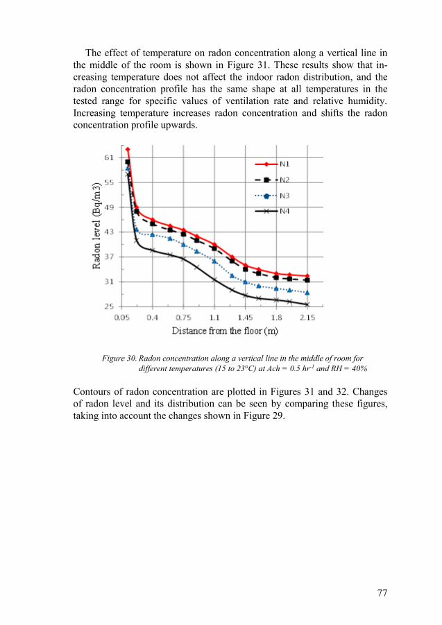
77
The effect of temperature on radon concentration along a vertical line in the middle of the room is shown in Figure 31. These results show that in-creasing temperature does not affect the indoor radon distribution, and the radon concentration profile has the same shape at all temperatures in the tested range for specific values of ventilation rate and relative humidity. Increasing temperature increases radon concentration and shifts the radon concentration profile upwards.
Figure 30. Radon concentration along a vertical line in the middle of room for different temperatures (15 to 23°C) at Ach = 0.5 hr-1 and RH = 40%
Contours of radon concentration are plotted in Figures 31 and 32. Changes of radon level and its distribution can be seen by comparing these figures, taking into account the changes shown in Figure 29.

78
Figure 31. Contours of radon concentration (Bqm-3) in two vertical planes in the middle of room for N3 (Ach = 0.5 hr-1, T = 21 °C, RH = 40%)
Figure 32. Contours of radon concentration (Bqm-3) in two vertical planes in the middle of room for N4 (Ach = 0.5 hr-1, T = 23 °C, RH = 40%)

79
5.4.3 Effects of Relative Humidity Changes on Indoor Radon Concentration
In order to investigate the effects of relative humidity changes on indoor radon concentration, six cases have been considered: N6, N4, N7, N8, N9 and N10, as listed in Table 9. Ventilation rate and temperature are fixed at 0.5 hr-1 and 21 °C respectively. Relative humidity is varied between 30 % and 80%. The model is solved for these cases as described in previous sec-tions and the results are shown in Table 22.
Table 22. Average radon concentration for different relative humidity at Ach = 0.5 hr-1 and T = 21 °C
Case No. Relative humidi-ty (%)
Average radon concentration (Bqm-3)
N6 30 39.17 N4 40 39.22 N7 50 39.25 N8 60 39.08 N9 70 39.82 N10 80 39.07
Table 22 shows that relative humidity does not have a large effect on aver-age indoor radon concentration. The negligible differences observed are due to numerical approximations and rounding.
This simulation is more accurate than the previous simulation presented for Ach = 0.25 hr-1 and T = 18 °C in Paper III because of the increase in mesh size (number of cells).
Contours of radon concentration at different relative humidity are plotted in Figures 33 and 34. These figures indicate that relative humidity changes between 30 % and 80 % have considerable impacts on indoor distribution. Even though the overall average radon level does not change with RH, these figures indicate that a change in relative humidity from 40% to 50% has an effect on indoor radon distribution, i.e. humidity variations can affect radon distribution in the occupied zone.

80
Figure 33. Contours of radon concentration (Bqm-3) in two vertical planes in the middle of room for N4 (Ach = 0.5 hr-1, T = 21 °C, RH = 40%)
Figure 34. Contours of radon concentration (Bqm-3) in two vertical planes in the middle of room for N7 (Ach = 0.5 hr-1, T = 21 °C, RH = 50%)

81
Model validation and result comparison
Model validation is performed by inter-model validation (Paper II) and com-parison with analytical solutions and measurements.
In a ventilated room, the radon diffusion coefficient is disregarded and radon concentration in a chamber (room) with volume V is described as per Equations (3.3) to (3.5).
In this study, the average radon concentration in Room 1 is calculated for the four considered air change rates using the analytical solution. For in-stance, at 0.5 Ach Equation (3.4) gives:
𝐶𝐶0.5 ℎ𝑟𝑟−1 =0.018 𝐵𝐵𝐵𝐵
𝑚𝑚2𝑠𝑠2.4 𝑚𝑚 × 0.5 1
ℎ𝑟𝑟 × 1 ℎ𝑟𝑟3600 𝑠𝑠
= 54 𝐵𝐵𝐵𝐵𝑚𝑚3
Table 23 shows a comparison of average concentrations in Room 1 at differ-ent air change rates using measurements, analytical calculation and numeri-cal simulation techniques. The measurement data are not sufficiently accu-rate for these comparisons, because the measuring time was too short to ob-tain an acceptable average radon level and the measurement devices have at least 10 percent uncertainty.
For quantitative comparisons, the percentage difference between the FLUENT estimation results and the analytical calculations was computed at each ventilation rate. The maximum difference was found to be less than 10%.
In spite of the errors in each technique, such as the 10 % uncertainty in the measurements by the CRM, the results show good agreement, thus veri-fying the model.
Table 23. Indoor radon levels obtained by different methods
Ventilation rate (hr-1)
Measurement (𝐁𝐁𝐁𝐁𝐦𝐦−𝟑𝟑)
Analytic (𝐁𝐁𝐁𝐁𝐦𝐦−𝟑𝟑)
Numeric (Bqm-3)
1.0 25±2 22 20.57 0.5 45±4 54 40.06
0.25 97±10 108 82.08 0.05 3,580±380 3,378 2,828.55
Measurements and numerical methods were both used to examine radon variation with height (Figures 19 and 22). These results can also be used to validate the CFD model.
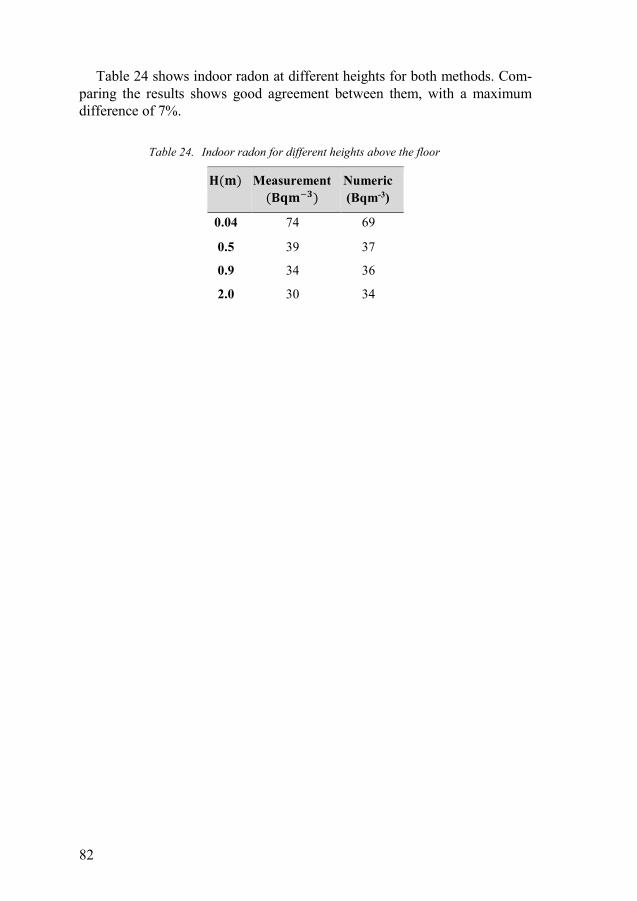
82
Table 24 shows indoor radon at different heights for both methods. Com-paring the results shows good agreement between them, with a maximum difference of 7%.
Table 24. Indoor radon for different heights above the floor
𝐇𝐇(𝐦𝐦) Measurement (𝐁𝐁𝐁𝐁𝐦𝐦−𝟑𝟑)
Numeric (Bqm-3)
0.04 74 69
0.5 39 37
0.9 34 36
2.0 30 34

83
6 Conclusions and future work
This thesis describes an investigation of two important topics. The first topic considers the effect of heat energy recovery ventilation systems on radon distribution and energy savings. The second topic includes quantifying the influence of indoor air conditions and ventilation parameters on radon con-centration by means of numerical methods.
Based on the main objective of this study, it is concluded that a heat re-covery ventilation system can influence indoor radon level by controlling air ventilation rate, the pressure difference between indoors and outdoors, in-door temperature and relative humidity. In response to the research question, most of the investigated factors affect indoor radon concentration and distri-bution and there is a strong correlation between these factors and indoor radon distribution. It is worth noting that indoor radon level can be influ-enced by concurrent outdoor conditions such as wind, rainfall, pressure and geological conditions as well as the examined indoor factors. For this reason CFD is a useful and applicable tool for investigating these factors individual-ly, and in this study it is used as a standalone and available tool to simulate and predict radon level and distribution in residential buildings. The conclu-sions of this study are described below.
Dynamic simulation and heat recovery analysis
The first set of conclusions considers the use of a balanced HRV system and its effect on IAQ with respect to radon concentration. Providing a balance between supply air and exhaust air and maintaining indoor air temperature and relative humidity by means of a HRV unit helps to control indoor radon. The dynamic simulations and theoretical analysis carried out here confirms that the use of a heat exchanger enhances the energy performance of a resi-dential ventilation system.
From an IAQ point of view, increased ventilation is one possible action to mitigate high radon levels. HRV systems can recover energy that would otherwise be lost through increased ventilation and reduce investment pay-back time. Nevertheless, increased ventilation is not recommended as the primary cost-effective mitigation measure, but rather as a complementary

84
one. Remediation actions such as floor sealing and creation of a radon sump deliver superior performance, as shown in the main body of this thesis.
Numerical Simulation
Numerical simulation is a valuable, powerful and inexpensive tool for as-sessing the behavior of harmful contaminants like radon, and for predicting indoor air flow at low cost and relatively quickly in comparison with other methods such as gas tracer and full-scale laboratory methods.
Three dimensional models developed in FLUENT were used to simulate radon entry and exit in a one-family house. The verification of the model and its performance reinforce the idea that radon transport in the house and ven-tilation effects have been well defined physically and numerically. The per-formance and sensitivity of the model were confirmed by varying some of the internal and boundary conditions. The results indicate that the considered conditions and assumptions provide a reliable illustration of the actual condi-tions. This model is therefore likely to be useful and applicable for other similar indoor radon problems with a similar range of conditions.
This study demonstrates that indoor radon level and distribution can gen-erally be affected by indoor air conditions such as temperature, relative hu-midity, ventilation rate and location. The impacts of these parameters on indoor radon level and distribution are summarized in Table 25.
Table 25. The impacts of parameters on indoor radon level and distribution
Parameters Indoor radon level Indoor radon distribution
Ventilation rate High impact, the more ventilation rate the lower the radon level
High impact
Supply air terminal device location
High impact, the closer to vent the lower the radon level
High impact
Room height High impact, the closer to the floor, the higher the radon level
High impact
Indoor temperature
Low impact, with direct correlation Low impact, considerable for occupied zone
Indoor relative humidity
No impact Low impact, considerable for occupied zone

85
Overall, the results indicate that indoor radon concentrations and dispersion are dependent on radon production rate, ventilation specifications and indoor temperature and humidity conditions. In addition, height above the floor, air infiltration through the main door and windows as well as location of the supply air terminal devices all impact indoor radon level.
Locating supply air terminal devices near the occupied zone in a new building could be a good means of controlling radon level.
Numerical results show that outdoor ventilation rate is the most influen-tial, indoor temperature is less influential and humidity is the least influential factor on indoor radon.
It should be emphasized that this work represents the first step in the field with regard to using CFD to study the sensitivity of indoor radon level and its distribution in small residential buildings. It is hoped that the present study will serve as a stepping stone for further work in the field by other researchers.
Future work
This thesis focuses on the study of ventilation effects of indoor temperature and humidity on indoor radon mitigation in a residential building, with em-phases on IAQ and energy saving approaches. The work could be extended in the future with more detailed three dimensional modeling of the building, which may increase the accuracy of the results.
Some further suggestions for future work include:
1. Modeling of novel energy recovery ventilation systems. 2. External coupling between CFD and BES (Building Energy Simulation)
software is likely to be a suitable approach for improving both the simu-lation results and the calculation of energy balance.
3. Considering outdoor air conditions such as pressure, temperature, and precipitation on indoor radon.
4. Consideration of air leakage from the building, internal heat sources, furniture and residents in models of indoor radon.
5. Investigation of the effectiveness of alternative supply air locations from a radon mitigation viewpoint.
6. Further comprehensive and systematic radon measurements in residen-tial buildings including tight control (where possible) of all factors that affect the measurement results. Such measurements are paramount for validating detailed CFD simulations and confirming new engineering findings.
7. There is a strong demand for comprehensive and systematic radon measurements in buildings including detailed control of all factors re-garding the building, etc. that also represent important input data for cal-

86
culations. CFD with its many possibilities can be useful for finding the best and most economical measure against radon in specific cases, i.e. optimization. However, there is a fundamental limitation when the cal-culation results cannot be compared with, and thus confirmed by de-tailed measurement results.
8. Derivation of simplified/analytical correlations or models for indoor temperature and relative humidity using CFD results.
87
References
Abd Alnasser Almate, A. A. (2014). Use of Computational Fluid Dynamics. American Journal of Engineering and Applied Sciences,7, pp. 171–184.
Akander, J., Alvarez, S., & Johannesson, G. (2005). Energy Normalization Techniques in Energy Performance of residential buildings: a practical guide for energy rating and efficiency. London ; Sterling, VA : Earthscan.
Anderson, C. E. (2001). Numerical modeling of radon-222 entry into houses: an outline of techniques and results. The science of total environment, 272, pp. 33–42.
ANSYS Inc. (2011). ANSYS FLUENT 14.0 Theory Guide. Canonsburg: ANSYS Inc. ASHRAE. (2001). Ventilation for Acceptable Indoor Air Quality. Atalanta:
ASHRAE. Bakker, A. (2010). Computational Fluid Dynamics. Retrieved 25.2.2012, from
Bakker: www.bakker.org/dartmouth06/engs150/05-solv.pdf Chauhan, N., Joshi, M., & Agarwal, T. (2014). Study of indoor radon distribution
using measurements and CFD modeling. Journal of Environmental Radioactivity,136, pp. 105–111.
Clavensjö, B., & Åkerblom, G. (1994). The Radon Book. Stockholm: The Swedish Council for Building Research.
Cozmuta, I., Van der Graff, E., & de Meiter, R. (2003). Moisture dependence of radon transport in concrete: Measurements and modeling. Health Physics, 85 (4), pp. 438–56.
Cussler, E. (1997). Diffusion: Mass Transfer in Fluid System. New York: Cam-bridge University Press.
Dainius, J., & Aloyzas, K. (2007). Hourly Measurement Method For Radon Progeny. Journal of Environmental Engineering, 15 (3), pp. 158–165.
Dubois, G. (2005). An overview of radon servey in Europe. Luxembourg: European Communitis. Retrieved 10.4.2013, from http://www.academia.edu
EPA. (2008). citizensguide. Retrieved 28.6.2011, from epa: www.epa.gov/radon/pdfs/citizensguide.pdf
Flexit. (2009). products/air-handling-units/. Retrieved 5.7.2013, from Flexit: http://www.flexit.no/en/products/air-handling-units/Old-models/
Fournier, F., Groetz, J., & Jacob, F. (2005). Simulation of Radon Transport through Building Materials. Trans Porous Med (59), pp. 197–214.
Gerasimov, A. (2006). Modeling Turbulent Flows with FLUENT. London: Europe, ANSYS Inc.
Handel, C. (2011). Ventilation with heat recovery is a necessity in “nearly zero” energy buildings. REHVA European HVAC Journal(3), pp. 18–22.
Hjelte, I., Ronquist, B., & Ronnqvist, T. (2010). The radon situation in Swedish dwellings based on recent measurements. Helsinki: European IRPA Congress.
Jokisalo, J., Kurnitska, J., & Torkki, A. (2003). Performance of balanced ventilation with heat recovery in residential buildings in cold climate. International Journal of Ventilation, 2, pp. 223–236.

88
Keith S, D. J. (2012). Toxicological Profile for Radon. Atlanta (GA): Agency for Toxic Substances and Disease Registry (US).
Keskikuru, T., Kokotti, H., Lammi, S., & Kalliokoski, P. (2001). Effect of various factors on the rate of radon entry into two different types of houses. Building and Environment, 36 (10), pp. 1091–1098.
Kumar, A., Chauhan, R., & Sahoo, B. (2014). Modeling of indoor radon concentration from radon exhalation rates of building materials and validation through measurements. Journal of Environmental Radioactivity,127, pp. 50–55.
Langtry, R. G. (2006). Predicting 2D airfoil and 3D wind turbine rotor performance using a transition model for general CFD codes. 44th AIAA Aerospace Sciences Meeting and Exhibit. Reno: AIAA.
Laverge, J., & Janssens, A. (2012). Heat recovery ventilation operation traded off against natural and simple exhaust ventilation in Europe by primary energy factor. Energy and Buildings, (50), pp. 315–323.
Lazzarin, R. M., & Gasparella, A. (1998). Thechnical and economical analysis of heat recovery in building ventilation systems. Applied thermal engineering, 18, pp. 47–67.
Lide, D. (2004). CRC Handbook of chemistery and physics. Florida: CRC press. Loureiro, C. (1987). Simulation of the steady-state transport of radon from soil into
houses with basement under constant negativepressure. Berkeley, CA.: Lawrence Berkeley Laboratory.
Malanca, A., Cassoni, F., Dallara, G., & Pessina, V. (1992). Radon in dwellings: the importance of ventilation. AEROBIOLOGIA, 8, pp. 57–61.
Marley, F., & Paul, S. (2001). Investigation of the potential for radon mitigation by operation of mechanical systems affecting indoor air. Environmental Radioactivity, 54, pp. 205–219.
Menter, F. R. (2006). Transition Modelling for General Purpose CFD Codes. Flow, Turbulence and Combustion, 77,1, pp. 277–303.
Milner, J., Dimitroulopoulou, C., & ApSimon, H. (2004). Indoor concentrations in buildings from sources. London: UK Atmospheric Dispersion Modelling Liaison Committee.
Motaman, S. (2013). High-speed imaging and computational modelling of close-coupled gas atomization. Journal of Computers & Fluids, 88, pp. 1-10. Retrieved 9.8.2014, from http://etheses.whiterose.ac.uk/6430/
Mourshed, M. (2012). Relationship between annual mean temperature and degree-days. Energy and Buildings, 45, pp. 418–425.
Narula, A. K., Saini, R., Goyal, S. K., & Chauhan, R. P. (2009). Indoor Radiation Levels Enhanced by Underground Radon Diffusion. Asian Journal of Chemistry, 21 (10), pp. 275–278.
Nilsson, P. E. (2006). Achieving the desired indoor climate. Lund: Commtech Group.
Oman, R. (2011). Energy and Buildings. Vasteras: Malardalen University. Petropoulos, N. P., & Simopoulos, S. E. (2001). Building materials radon exhalation
rate. The Science of the Total Environment , 272, pp. 109–118. Radiological Protection Institute of Ireland. (2010). RPII. Retrieved 12.7.2012, from
www.epa.ie/pubs/reports/radiation/RPII_Guide_Radon_Remediation_Householders.pdf
Radonelektronik. (2009, 4 7). programvara. Retrieved 2 12, 2010, from Radonelektronik: http://www.radonelektronik.se/programvara.htm
Revzan, K. (2008). Modeling Radon Entry into Houses with Basements: Model Description and Verification. Lawrence Berkeley: Lawrence Berkeley National Laboratory, LBNL .
89
Shao, J. L. (2010). Field Measurement of the Convective Heat Transfer Coefficient on Vertical External Building Surfaces Using Naphthalene Sublimation Method. Journal of Building Physics, 33 (4), pp. 307–326.
Sonntag, D. (1990). Important new values of physical constants of 1986, vapour pressure formulations based on the ITS-90 and PsychrometerFormulae. Viena: Zeitschrift fur Meteorologie.
Spoel, W. V. (1998). Radon transport in sand: A laboratory study. Eindhoven, Netherland: Eindhoven University of technology.
Sundal, A., Henriksen, H., Lauritzen, S., & Soldal, O. (2004). Geological and geochemical factors affecting radon concentrations in dwellings located on permeable glacial sediments — a case study from Kinsarvik, Norway. Environ Geol, 45, pp. 843–858.
Swedish Energy Agancy. (2010, 1 31). Energy in Sweden. Retrieved 4 10, 2013, from www.energymyndigheten.se.
Wang, F., & Ward, I. C. (2000). The development of a radon entry model for a house with a cellar. Building and Environment, 35, pp. 615–631.
Wang, F.; Ward, I C. (2002). Radon entry, migration and reduction in houses with cellars. Building and Environment, 37, pp. 1153 – 1165.
Versteeg, H., & Malalasekera, W. (2007). An introduction to Computational Fluid Dynamics: The Finite Volume Method. Glasgow: Pearson.
White, F. M. (2011). Fluid Mechanics. New York: McGraw-Hill. WHO. (2009). WHO handbook on indoor radon: a public health perspective.
Geneva: WHO. Retrieved from http://www.who.int/mediacentre/factsheets/ fs291/en/index.html.
William, L. R. (1990). Toxicological profile for radon. New York: U.S. Public Health Service, in collaboration with U.S. Environmental Protection Agency. Retrieved 12.4.2010, from http://www.bvsde.paho.org/bvstox/i/fulltext/ toxprofiles/radon.pdf
Wunderground. (2010). MonthlyHistory. Retrieved 30.6.2014, from wunderground: http://www.wunderground.com/history/airport/ESSA/2010/12/1/ MonthlyHistory.html
Zhang, F., & Cooke, P. (2010). Green-building-review. Retrieved 27.3. 2013, from Dime: http://www.dime-eu.org/files/active/0/Cooke-2010-Fang-Green-building-review.pdf
Zhang, Y. (2004). Indoor air quality engineering. Illinois, Urbana: CRC press. Zhuo, W., Iida, T., Moriizum, J., & Takahashi, I. (2001). Simulation of the
concentrations and distributions of indoor radon and thoron. Radiation Protection Dosimetry, 93 (4), pp. 357–368 .

90

91
Appendices

92

93
Appendix A: IDA, Boundary conditions and input data
This appendix shows the results of dynamic simulation carried out by IDA Indoor Climate and Energy software program.
Table A1 shows project data and case study house specifications.
IDA Indoor Climate and Energy Version: 4.51 License: IDA40:ED152/R4N4Q (educational license)
\
Table A1. Project data and case study house specifications.
Energy report for "Air Handling Unit"
Project Building
Model floor area 108.0 m2
Customer H. Afshar Model volume 259.3 m3
Created by
K. Akbari Model ground area 0.0 m2
Location Stockholm/Bromma Model envelope area 208.8 m2
Climate file
Stockholm, Brom-ma-1977
Window/Envelope 2.6 %
Case 0.5 ach hex unit SL4, 0.74 etta sup-ply air 16degree
Average U-value 0.4071 W/(K·m2)
Simulated 8/3/2014 23:28:14 Envelope area per Volume 0.8055 m2/m3

94
Table A2 shows data base of climate data which is used for energy simula-tion and calculation.
Climate file
Dry-bulb tem-perature, Deg-C
Rel humidity of air, %
Direction of wind, Deg
Speed of meteorologi-cal wind, m/s
January -2.0 88.4 163.4 3.3
February -4.7 83.8 177.9 3.1
March 0.9 76.1 181.2 3.5
April 2.7 73.5 181.8 3.7
May 10.3 64.5 151.8 3.5
June 15.5 64.3 154.0 3.2
July 14.8 76.4 174.4 3.2
August 15.2 74.5 149.1 2.4
September 9.7 74.5 210.2 3.3
October 7.7 83.9 198.5 3.3
November 3.6 87.4 204.5 3.8
December -0.1 86.0 192.8 4.0
mean 6.2 77.8 178.2 3.3
mean*8760.0 h 54291.5 681313.2 1561105.0 29345.5
min -4.7 64.3 149.1 2.4
max 15.5 88.4 210.2 4.0
Table A2. Climate data in IDA data base

95
The geometry of the case study house is as follows.
Figure A1: Building geometry
Air handling unit (AHU) temperature for the year 2010 is as follows.
Figure A2. Air handling unit temperature
Return air dry-bulb temperature, Deg-CSupply air dry-bulb temperature, Deg-COutside air dry-bulb temperature, Deg-C
0 1000 2000 3000 4000 5000 6000 7000 8000
Jan Feb Mar Apr May Jun Jul Aug Sep Oct Nov Dec
°C
-15
-10
-5
0
5
10
15
20
25
Entire simulation: from 1/1/2010 to 12/31/2010

96
Energy report for "Air Handling Unit" including heat recovery and fans en-ergy use at 0.5 Ach is as follows.
kWh (sensible and latent)
Month Heating Cooling AHU heat re-covery
AHU cold re-covery
Humidi-fication Fans
Total 0.0 0.0 3380.6 22.7 0.0 613.5
Table A3. Energy report for "Air Handling Unit"

97
Appendix B: Radon Transport Equations and Indoor Conditions
1. Radon transport equation in the soil (when diffusion mechanism is dominant) In a one dimensional problem under certain conditions, such as in the area infinitely distant from the pressure disturbance, the radon transport equation, Equation 4.5, has an analytical solution for diffusion term. Using z as a spa-tial variable (0 ≤ 𝑧𝑧 ≤ ∞) and 𝑉𝑉 = 0, this equation is reduced to:
𝐷𝐷 𝑑𝑑2𝐶𝐶𝑑𝑑𝑧𝑧2 − 𝜆𝜆𝑅𝑅𝑅𝑅𝐶𝐶 + 𝐺𝐺 = 0 (B1)
This boundary condition is known as the infinite distant boundary. The re-sults of the differential equation solution can be compared with the solution using the numerical results at this boundary to assess the validity of the model.
To solve this equation, assuming that 𝑋𝑋 = 𝐺𝐺 − 𝜆𝜆𝑅𝑅𝑅𝑅𝐶𝐶, gives the following equation:
𝐷𝐷 𝑑𝑑2𝑋𝑋𝑑𝑑𝑧𝑧2 − 𝜆𝜆𝑅𝑅𝑅𝑅
𝐷𝐷 𝑋𝑋 = 0 (B2)
Therefore the solution of this differential equation is:
𝑋𝑋 = 𝛼𝛼1𝑒𝑒𝑒𝑒𝑒𝑒 (√𝜆𝜆𝑅𝑅𝑅𝑅𝐷𝐷 𝑧𝑧) + 𝛼𝛼2𝑒𝑒𝑒𝑒𝑒𝑒 (−√𝜆𝜆𝑅𝑅𝑅𝑅
𝐷𝐷 𝑧𝑧),
and 𝐶𝐶(𝑧𝑧) = 𝛼𝛼1𝜆𝜆𝑅𝑅𝑅𝑅
𝑒𝑒𝑒𝑒𝑒𝑒 (√𝜆𝜆𝐷𝐷 𝑧𝑧) + 𝛼𝛼2
𝜆𝜆𝑅𝑅𝑅𝑅𝑒𝑒𝑒𝑒𝑒𝑒 (−√𝜆𝜆𝑅𝑅𝑅𝑅
𝐷𝐷 𝑧𝑧) + 𝐺𝐺𝜆𝜆𝑅𝑅𝑅𝑅𝜆𝜆 (B3)
To solve this differential equation, considering boundary condition (at 𝑧𝑧 =0 𝑎𝑎𝑅𝑅𝑎𝑎 𝑧𝑧 = ∞) results:
𝐶𝐶(𝑧𝑧) = 𝐺𝐺𝜆𝜆𝑅𝑅𝑅𝑅
(1 − 𝑒𝑒𝑒𝑒𝑒𝑒 (−√𝜆𝜆𝑅𝑅𝑅𝑅𝐷𝐷 𝑧𝑧)) (B4)
where
𝐶𝐶(0) = 0 and 𝐶𝐶(∞) = 𝐺𝐺𝜆𝜆𝑅𝑅𝑅𝑅
= 𝐶𝐶𝑚𝑚𝑚𝑚𝑚𝑚𝑚𝑚𝑚𝑚𝑚𝑚𝑚𝑚.

98
Radon generation rate (𝐺𝐺) is a function of radium activity(𝐴𝐴𝑅𝑅𝑅𝑅), soil porosi-ty (𝜀𝜀), soil density (ρ)and emanation factor (𝑓𝑓)which is expressed as fol-lows:
𝐺𝐺 = 𝐴𝐴𝑅𝑅𝑅𝑅ρ𝑓𝑓 1−𝜀𝜀𝜀𝜀 (B5)
This solution shows that if the pressure disturbance is zero, the radon con-centration along the boundary depends only on the diffusion coefficient and the radon decay constant.
2. Diffusion length One of the variables in radon transport is radon diffusion length, which de-pends on soil and materials structure.
For a one dimensional problem, using z as the spatial variable (0 ≤𝑧𝑧 ≤ ∞), radon diffusion length can be derived from Equation B4:
𝐶𝐶(𝑧𝑧) = 𝐺𝐺𝜆𝜆𝑅𝑅𝑅𝑅
(1 − 𝑒𝑒(−𝑧𝑧𝑙𝑙 )) (B6)
𝑙𝑙 = √𝐷𝐷 𝜆𝜆𝑅𝑅𝑅𝑅⁄ (B7)
where 𝑙𝑙 is radon diffusion length (m), D is radon diffusion coefficient (m2s-1) and 𝜆𝜆𝑅𝑅𝑅𝑅 is radon decay constant (2.1 × 10⁻⁶𝑠𝑠−1). The diffusion length is defined as the characteristic distance travelled by radon atoms during one half life.

Papers


Paper I


Impacts of heat recoveryventilators on energy savings
and indoor radon levelKeramatollah Akbari
School of Sustainable Development of Society and Technology,Malardalen University, Vasteras,
Sweden and Technology Development Institute, ACECR, Tehran, Iran, and
Robert OmanSustainable Development of Society and Technology,
Malardalen University, Vasteras, Sweden
Abstract
Purpose – This paper aims to investigate the impact of heat recovery ventilators (HRVs) on theenergy use and indoor radon in a one family detached house. Heat recovery ventilation systems,because of reducing ventilation loss through recovered exhaust air, can play a good role in theeffectiveness of ventilation to reduce energy use. In addition HRVs can maintain pressure balance andoutdoor ventilation rate at a required level to mitigate indoor radon level.Design/methodology/approach – In this study, a multizone model of a detached house is developedin IDA Indoor Climate and Energy (IDA ICE 4.0). The model is validated using measurementsregarding use of energy for heating, ventilation and whole energy use. The performance of the heatrecovery ventilation system is examined with respect to radon mitigation and energy saving bymeasuring the radon concentration and analyzing the life cycle cost of a heat exchanger unit.Findings – The results of the measurements and dynamic simulation showed that the heat recoveryventilation system could lead to 74 per cent energy savings of the ventilation loss, amounting to about30 kWh m�2 per year. Life cycle cost analysis used for assessing total costs and the result showed thatusing this system is quite cost-effective and investment would payback during 12 years.Research limitations/implications – Limitations of this study generally refer to radonmeasurement and simulation because of radon complex behavior and its high fluctuations evenduring short periods of time.Practical implications – Heat recovery ventilation systems with reducing radon concentrationimprove indoor air quality and decrease environmental problems with energy savings.Social implications – Using balanced heat recovery ventilation can have benefits from theviewpoint of environmental impacts and household economy.Originality/value – Employment of a heat recovery unit to control indoor radon level is a new usageof this technology which along with energy savings can improve sustainable development.
Keywords Heat recovery, Ventilation, Energy saving, Radon, Indoor Climate and Energy (IDA 4.0)
Paper type Case study
NomenclatureA0 initial investmentB0 all savings in net present value methodB annual savings in monetary unitcp heat capacity (KJ kg�1 1C�1)EHex ventilation loss with heat exchangerErec recovered energy (kWh)Ev ventilation loss (kWh)Gt heat degree hours
The current issue and full text archive of this journal is available atwww.emeraldinsight.com/1477-7835.htm
Management of EnvironmentalQuality: An International JournalVol. 24 No. 5, 2013pp. 682-694r Emerald Group Publishing Limited1477-7835DOI 10.1108/MEQ-06-2012-0050
682
MEQ24,5

i interest rateMwater water mass (kg).m mass flow (kg s�1)n time in year unitQv specific ventilation loss (w 1C�1)q annual energy cost escalation ratet temperature (1C)V volume (m3)Z temperature efficiencyl radon decay rate (h�1)lv ventilation rate (h�1)r air density
1. IntroductionEnergy consumption in the building sector continues to grow steadily, and makes uparound 40 percent of total energy consumption in many countries (Kaberger et al.,2009). Therefore measures of reduction building energy use are a major concern.
In 2007, Swedish Energy Agency reported that electricity use between households,varying from 2000 to 7000 kWh per year for a detached house, and about 61 percentof energy use in this sector is used for space heating and domestic hot water (Kabergeret al., 2009; Swedish Energy Agency, 2009). In Sweden, heat recovery fromexhaust ventilation in existing buildings is an approach to reduce total energy use perheated area up to 20 percent below 1995 levels by 2020 (Ministry of SustainableDevelopment, 2006).
Energy in buildings is used to overcome the heat losses due to the ventilation,infiltration and transmission through the buildings envelope. The energy performanceof buildings is significantly affected by ventilation and generally accounts for 30-60percent of the buildings energy use (Awbi, 1998).
The prevalence of heat recovery ventilators (HRVs) systems in residential buildingsin Sweden has increased over the last few decades. The increase in energy efficiencythrough heat recovery systems such as these contributes to a more sustainable society.
A heat recovery unit because of saving energy and reducing radon level has twodifferent useful performances. The aim of this study is to show the effectiveness ofHRV systems for reducing energy consumption and controlling indoor radon level dueto balances between incoming and outgoing air streams.
Using HRV systems can help many of the more than 500,000 dwellings in Swedenwhich suffer from elevated radon concentrations in the range 200-800 Bqm�3, and the1,000,000 dwellings that have radon concentrations of 100-200 Bqm�3 (Swedjmark andMjones, 1987), which need increased ventilation to reduce indoor radon concentrations.Besides of energy use concerns in building sector, more than 30 percent of Swedishresidents live in dwellings which have radon levels above safe level, i.e. 100 Bqm�3,which requires remedial actions (Zeeb and Shannoun, 2009).
Since large volumes of Swedish bedrock consist of uranium-rich graniteand pegmatite, radon level is much higher than an action level (Swedjmark andMjones, 1987). Radon gas decays into metal ions which produce a-particles. Breathingthese particles are harmful for human body air ways and lead to lung cancer (Zeeb andShannoun, 2009).
Several studies have compared various ventilation systems to show the advantagesof heat recovery systems in cold climates ( Jokisalo et al., 2003). One of these studies
683
Heat recoveryventilators

showed that energy efficiency could be improved by up to 67 percent compared to atraditional exhaust ventilation system by using a heat recovery system with a nominaltemperature efficiency of 80 percent ( Jokisalo et al., 2003; Turiel et al., 1983).
The best currently available system for reducing ventilation losses and controllingindoor radon is the recovery ventilator. A heat recovery unit with effectiveness at least50 percent can save large amount of energy and it can be economically veryadvantageous (Lazzarin and Gasparella, 1998).
Comparison between an exhaust fan and a heat recovery ventilation system in acold climate showed that a heat exchanger air-to-air ventilation system can save up to2710 kWh per year compared to a traditional ventilation system and space heating(Hekmat et al., 1986). This amounts to an increase in energy efficiency of around30 percent in an insulated house. This is the best current technology for reducingradon levels (Hekmat et al., 1986; Hubbard et al., 1996).
2. Methodology2.1 Materials and methodsThe investigation was conducted in a single-family detached house, where radon levelswere measured in conjunction with remedial changes to reduce these levels. A rotaryheat exchanger unit and radon detectors were employed to measure heat recoveryand radon level, respectively.
The radon measurement tools included a continuous radon monitor (CRM, R2)produced by Radonelektronik Company (Radonelektronik, 2009) which is an electronicdevise with 10 percent error and a-track detectors. Passive a-track detectors contain aplastic sheet of film onto which the a-particles produced from radon and radon progenyetch lines as they pass through the monitor. These etched lines are then analyzed in alaboratory and the radon concentration is quantified with 10 percent accuracy. Theheat recovery unit (Flexit SL4 R) is an air handling unit with rotor technology producedby Flexit Company (FLEXIT, 2009) with 80 percent nominal efficiency.
IDA indoor climate and energy (ICE) was used as a multizone dynamic simulationtool to predict energy consumption, heat recovery of the rotary heat exchanger unitanalysis, simulation of thermal comfort and indoor air quality in buildings. Researchmethods applied in this study include analytical analysis, measurement, dynamicsimulation and life cycle cost analysis.
2.2 Case study descriptionThe building selected for case study is a detached one family house in Stockholm builtin 1975. This house is a two-storey structure with a volume of about 259m3 on eachlevel. This corresponds to a floor area of about 108m2, windows (W1, W2 andW3) area8.8m2, main door (D1) area 3.3m2 and internal door(s) area 2.2m2. Some parts of thishouse was renovated and sealed in order to energy conservation and radon reduction.This house is situated on bedrock and major radon gas originates from the floor.
Total energy purchased were 25,860 and 22,920 kWh per year before and afterusing heat recovery ventilation system, respectively. Figure 1 shows the floor plan ofthis house.
3. The heat recovery ventilation systemAmechanical ventilation system with an air-to-air heat exchanger unit provides the airsupply to the first floor. Figure 2 illustrates incoming and the outgoing air streams theinstalled heat exchanger system inside the first storey.
684
MEQ24,5

The operating points of the unit can be determined from the diagram shown inFigure 3. The operating points at 0.5 and 1.0Ach are shown with the orange dashedand continuous lines, respectively in Figure 3.
Given the ventilation rates and Figure 3, it is possible to find the operating ratessuch as pressure, noise and fan(s) electrical energy consumption. The unit efficiencywas derived from Equation (1) as shown below, and the determined values are shownin Table I.
Temperature efficiency Z (Taniplan, 2009):
Z ¼ ðt12 � t11Þ=ðt21 � t11Þ ð1Þ
This unit provides the outdoor air at three levels, i.e. 0.25, 0.5 and 1Ach. At a particularinstance, the outdoor and the indoor conditions (t11, t21, RHOutdoor, RHIndoor) weremeasured through Equation (1).
According to the manufacturer, the maximum temperature and relative humidity(RH) efficiencies of this rotary heat exchanger unit are 80 percent (FLEXIT, 2009).
F11F11
F12
F12
B1
B1 Supply air temperaturesensor
Supply air filter
Supply air fanExtract air fanRotary wheel-typeheat exchangerRotor motor
Extract air filter
Heating elementOverheating thermostat,
Overheating thermostat,MANUAL RESET
AUTOMATIC RESET
F20
F20
F10
F10
EB1
EB1
HR-R
HR-R
Extract airt22 t12 t11 t21
M2
M2
M4M4
M1
M1
Supply air Outdoor air Exhaust air
Source: Taken from FLEXIT Company
Figure 2.Schematic diagramof the rotary heat
exchanger installedin the building
W2 W1
W3
D1D2
Livingroom 4 m
6 m
4 m
4 m
Hall
WC
Dressingroom StoreSauna
Bedroom
Bedroom
5 m
3 m3 m 2 m
Figure 1.Ground floor plan
and zone divisions ofthe case study house
685
Heat recoveryventilators

These values are not always reached, as demonstrated below:
Zt ¼ ð14:5þ 7:4Þ=ð22þ 7:4Þ ¼ 74:5%
This unit can use two types of fans, alternative current (AC) and direct current (DC).The fans mechanical efficiency or specific fan power (SFP) for AC and DC fansare calculated 9.7 and 5.5 kW per cubic meter per second at 0.5 Ach, respectively.This means that mechanical efficiency of an AC fan is about 0.56 percent lower thanof a DC fan.
As shown in Figure 3, the AC fan power at 0.5 Ach is about 35W and the annualenergy use of two fans (supply and exhaust fans) would be 613 and 350 kWh for ACfans and DC fans, respectively.
400
300
0 W
5035
100
150
200
80
200
100
Pα015
125
0 100 2000.5 Ach 1 Ach 300 400
Notes: 1, Capacity curves (blue); 2, operation curves (black); 3, power consumption curves(green); 4, sound curves (red); 5, operation points (orange)Source: (From FLEXIT Company; FLEXIT (2009)
190V
80dB(A)
83dB(A)
170V
75dB(A)70dB(A)
120V
65dB(A)
105V
60dB(A)
85V60V
230V
190V170V150V120V105V85V60V
m3/h
150V
Figure 3.Characteristics curves ofair supply AC fan
Specifications Operating rates
2 Fans power (max. 2� 165W) 70WTemperature efficiency 74.5%Ventilation rate 0.5Ach (35 l s�1)Noise 50 dBA
Table I.The operating ratesof the unit
686
MEQ24,5

4. Heat losses of the houseThermal losses in buildings are generally attributable to ventilation losses,transmission losses of the envelope and losses of domestic hot water. Ventilationlosses are increasing due to the new indoor air quality standards and the focus onreducing indoor radon concentration in cold climates. Reducing losses due toventilation are therefore expected to have a large impact on energy use. Calculations ofthe ventilation losses for this case study are as the following.
Ventilation losses are investigated using exhaust fan and heat recovery as aventilation system.
4.1 Using exhaust fanIt is assumed that the fan-driven supply air flow represents 90 percent of the fan-drivenexhaust air flow (a normal ratio leading to a low negative pressure indoors on average,which is an advantage when humidity is taken into account), temperature efficiency forthe heat exchanger 74 percent and air leakage in addition to fan-driven ventilationequal to 0.05Ach:
0:9�0:5 Ach�259m3 ¼ 116:55m3h�1 ¼ 0:04 kg s�1 ¼ 32:4 l:s�1
Total infiltration (air leakage) not affected by the heat exchanger is the sum of fan-driven infiltration (10 percent of the exhaust air flow) (Oman, 2011), and the air leakageat 0.05 Ach corresponding to air leakage both in and out in addition to fan-drivenventilation:
0:1�0:5 Ach�259m3 þ 0:05 Ach�259m3 ¼ 25:9m3:h�1 ¼ 7:2 l:s�1
Specific ventilation loss (Qv) is the sum of fan-driven supply air loss (Qs), and the totalinfiltration loss (Ql):
Qv ¼ Qs þ Ql ¼ S .m cp ð2Þ
where cp is the air heat capacity (1.01 KJ kg�1 1C�1) and.m is the mass flow (kg s�1)
Qv ¼ 39:4þ 8:7 ¼ 48 W:�C�1
Based on monthly long mean temperature in Stockholm (Worldclimate, 2009) andfixing room temperature at 201C, the heating degree days (HDDs) give 4,500 degreedays corresponding to 108,000 heat degree hours per year:
Ev ¼ Qv�Gt ð3Þ
where gt is the heat degree hours per year:
Ev ¼ 4254þ 938:5 ¼ 5;192 kWh per year
4.2 Using heat recovery systemThe heat exchanger reduces the heat demand by a factor (1�Zt). However, the heatexchanger only affects the fan-driven supply air (90 percent of the exhaust air).
687
Heat recoveryventilators

Equation (4) shows the energy demand of heating using heat exchanger:
QHex ¼ Qsð1� ZtÞ ð4Þ
QHex ¼ 10:24 W:�C�1
EHex ¼ 1106 kWh per year and Erec ¼ Es � EHex ¼ 3148 kWh per year
If it is considered, 0.25plvp1, 2,000pHDDp6,000 and 0.7pZtp0.85, annual energyrecovery is in the following ranges:
6pE recp90 kWhm�2; and for this case study Erec ¼ 30 kWhm�2:
Ventilation losses of the house are summarized in Table II. Normal condition isdefined as in which ventilation rate and infiltration rate are 0.5 and 0.05 Ach,respectively.
The other heat losses in the house are transmission loss and domestic hot waterloss. The calculation results of transmission and domestic hot water losses are 8,240and 3,186 kWh per year, respectively. This means that total heat loss for this house isabout 10,284 kWh per year.
5. Results5.1 Radon measurementsRadon concentrations were measured constantly during the winter. The measurementtools included a continuous radon meter (CRM) and a-track detectors (ATD). Table IIIshows the results of these measurements.
There are usually some errors in radon measurement, such as place of detectors,measuring period and electromagnetic fields for electronic radon meter. These factorscan affect on measurement results.
Heat loss typesSpecific heatloss (W 1C)
Energy(kWh per year)
Recovered energy(kWh per year)
Exhaust fan (0.5 Ach) 39.4 4,254 –HRV (0.5Ach) 10.2 1,106 3,148Air leakage (0.05 Ach) 8.7 938.5 –
Table II.Ventilation losses of thehouse at normal condition
Date and periodATD
(Bqm�3)CRM
(Bqm�3)Air changerate (h�1) Ventilation type Remedial action
2-2008 (2 weeks) 3,5807380 – 0.25 Exhaust fan No action2-10-2010 (1 week) – 150715 0.25 HRV 3 connected sumps3-18-2010 (12 days) – 6576 0.5 HRV 3 connected sumps4-22-2010 (12 days) – 3674 1 HRV 3 connected sumps
Table III.Radon measurementsresults
688
MEQ24,5

5.2 Analytical analysisIf it is assumed that the rate of the radon generation (G) is constant, then the radoncontent of the indoor radon can be calculated as:
C ¼ EA=VðlþlvÞ ð5Þ
where C(Bqm�3) accounts for the indoor radon at the steady state, E(Bqm�3 h�1) is therate of radon exhalation, A(m2) is the area of the radon exhalation surface (the floorarea in this case), V(m3) is the volume of the house, and lv (h
�1) is the ventilation rateof the house.
Using Equation (5) indoor radon can easily be calculated with E¼ 65 Bqm�3 h�1
(Clavensjo and Akerblom, 1994), and the given data from the case study of the housefor different ventilation rates. The results are as shown in Table IV.
It can be seen that measured data from Table III are comparable with the analyticalresults. The error between analytical analysis and measurement data is less than14 percent at 0.5 Ach.
In order to show the impact of the ventilation rate on the radon level, and to havea qualitative comparison, the radon concentrations were measured by means of a CRMinstrument at three different ventilation rates (Figure 4). However, this figure is notsuitable for a quantitative comparison due to the short measurement time.
5.3 Dynamic simulation resultsFor a long-term assessment of the heat recovery ventilation efficiency it is necessaryto consider the complete time series of outdoor temperature and all the losses and gainsof the building during the heating period.
Ventilation rate (Ach) Indoor radon (Bqm�3)
0.0 3,5820.25 1080.5 541.0 27
Table IV.Analytical resultsof indoor radon
0.5 Ach0.25 Ach
0.1 Ach
Bq
m–3
120110100
9080706050403020
12Time(hours)
24 48
Figure 4.Continuous radon
concentration levelsmeasured with CRM
689
Heat recoveryventilators

The variations in outdoor temperature and ventilation rate may change the heatrecovery temperature and humidity efficiencies. All these time-dependent effects weretaken into account through using dynamic thermal simulation programs. These resultsare explained in this section.
Table V shows delivered energy overview of the simulation results. In this table,delivered energy for ventilation is related to electrical energy for supply and exhaustfans and heating refers to thermal losses of the house.
These values are comparatively close with the calculation results as seen inSection 4.
The annual results of the IDA dynamic simulation are shown in Table VI. This tablecompares the heat recovery ventilation system with an exhaust (traditional) fanventilation system. Also using DC fan instead of AC fan can reduce electrical energymore than 50 percent.
The whole-year predicted result of the dynamic simulation is shown that the heatexchanger ventilation system can damp wide variations in the outdoor conditions andmaintain the indoor air at a set point temperature with a small variation throughout the year.
The results of measurement and simulation showed that increasing ventilationrates decrease indoor radon levels (inversely proportional) but raise ventilation energyuse (direct proportional). Table VII compares different ventilation rates, indoor radonlevels and total ventilation losses quantitatively.
5.4 Economic analysis5.4.1 Energy analysis. In order to install a radon mitigation system, the followingaspects should be considered: ventilation loss, cost of the operational energy and the
Ventilation rate(Ach)
Fans energy use(kWh)
Ventilation thermal energy use(kWh)
Radon level(Bqm�3)
0.25 350 2,630 1500.5 616 5,192 651 1,400 10,384 36
Table VII.Comparison betweenenergy use and radon level
Ventilationsystem
Air change rate(h�1)
Heat recovery(kWh)
AC fans energy use(kWh)
DC fans energy use(kWh)
Heat 1.0 7,163 1,227 514Recovery 0.5 3,506 616 352Ventilation 0.25 1,799 307 129Exhaust fan 0.5 0 4,368 –
Table VI.Simulation resultsof energy savings withdifferent ventilation rates
kWh kWhm�2
Domestic hot water 3,386 31Ventilation at 0.5Ach 616 8Heating at 0.5Ach 9,977 93
Table V.Delivered energy overview
690
MEQ24,5

future energy price, climate, fan(s) energy consumption, heat energy cost, indoor airtemperature and ventilation rate (dependent on the life style of the occupants) and theinitial and installation costs of the unit.
The heating and cooling degree day is a useful method which has been used inindustry and academia for many years (Akander et al., 2005).
In cold climates, high heating degree days are very important from the viewpointof the energy recovery when proposing the ventilation system for radon mitigation.The energy loss and the initial costs of a ventilation system to reduce radon levels areusually the main concerns of the home owners.
In order to install a radon mitigation system, some costs and key factors such as thedirect electrical energy cost, efficiency, noise and service lifetime of the ventilation unitshould be considered. Since the ventilation system is installed indoors, the size of thesystem is also a concern for the homeowners.
A general and accepted approach to calculate the recovered energy is the outsidetemperature cumulative curve during the heating and cooling period. The seasonalrecoverable energy at constant room temperature (201C) was calculated.
5.4.2 Energy life cycle cost analysis. The net present value (NPV) method was used toevaluate the cost-effectiveness of an investment in the future.
Life cycle costs consist of the initial capital investment, the installation costs of therotary heat exchanger unit, which is about 4,000 USD for this unit, and the energy andmaintenance costs. The annual electrical consumption of the unit is 616 kWh. Theannual cost of replacing two of the unit’s filters is about 80 USD.
For the NPV analysis, the following assumptions were considered:i¼ 4 percent, q¼ 2 percent, n¼ 25 years and energy cost in Sweden is roughly about
0.16 USD per kWh including all taxes.In this method if the NPV of all the savings is larger than the initial capital cost, an
investment is profitable (Nilsson, 2006).Based on analytical relations, the NPV of this heat recovery was calculated and
the results of the life cycle cost are shown in Table VIII. The life cycle cost analysisshows that the use of a HRV system is cost-effective, and with regard to the annualincrease of the energy cost, in this case the investment will have a payback period ofabout 12 years.
The annual energy saving varies with the ventilation rate; the amount of ventilationloss with and without the heat exchanger unit is shown in Figure 5. The two keyfactors which potentially add to the utility costs of a residential radon mitigationsystem are the outside environmental conditions and the house air exchange rate(Ach). Considering that there may be a 30-60 percent increase in energy consumptiondue to buildings ventilation (Awbi, 1998) and radon mitigation system, it is apparentthat a huge amount of energy can be saved through a heat recovery ventilation system.Therefore, employing this type of radon mitigation system is quite cost-effective.
Annual costs (USD)Ventilation system Capital cost (USD) Energy maintenance Life cycle costs (USD)
Traditional fan 100 702 – 13,605HRV with AC fan 4,000 98 80 7,488HRV with DC fan 4,000 56 80 6,655
Table VIII.Ventilation systems life
cycle cost analysis
691
Heat recoveryventilators
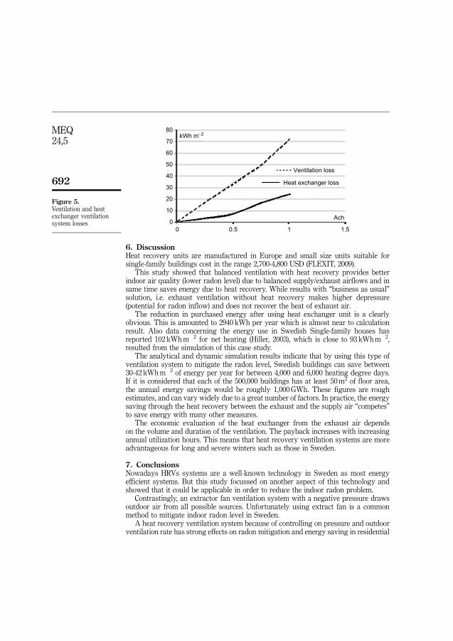
6. DiscussionHeat recovery units are manufactured in Europe and small size units suitable forsingle-family buildings cost in the range 2,700-4,800 USD (FLEXIT, 2009).
This study showed that balanced ventilation with heat recovery provides betterindoor air quality (lower radon level) due to balanced supply/exhaust airflows and insame time saves energy due to heat recovery. While results with “business as usual”solution, i.e. exhaust ventilation without heat recovery makes higher depressure(potential for radon inflow) and does not recover the heat of exhaust air.
The reduction in purchased energy after using heat exchanger unit is a clearlyobvious. This is amounted to 2940 kWh per year which is almost near to calculationresult. Also data concerning the energy use in Swedish Single-family houses hasreported 102 kWhm�2 for net heating (Hiller, 2003), which is close to 93 kWhm�2,resulted from the simulation of this case study.
The analytical and dynamic simulation results indicate that by using this type ofventilation system to mitigate the radon level, Swedish buildings can save between30-42 kWhm�2 of energy per year for between 4,000 and 6,000 heating degree days.If it is considered that each of the 500,000 buildings has at least 50m2 of floor area,the annual energy savings would be roughly 1,000GWh. These figures are roughestimates, and can vary widely due to a great number of factors. In practice, the energysaving through the heat recovery between the exhaust and the supply air “competes”to save energy with many other measures.
The economic evaluation of the heat exchanger from the exhaust air dependson the volume and duration of the ventilation. The payback increases with increasingannual utilization hours. This means that heat recovery ventilation systems are moreadvantageous for long and severe winters such as those in Sweden.
7. ConclusionsNowadays HRVs systems are a well-known technology in Sweden as most energyefficient systems. But this study focussed on another aspect of this technology andshowed that it could be applicable in order to reduce the indoor radon problem.
Contrastingly, an extractor fan ventilation system with a negative pressure drawsoutdoor air from all possible sources. Unfortunately using extract fan is a commonmethod to mitigate indoor radon level in Sweden.
A heat recovery ventilation system because of controlling on pressure and outdoorventilation rate has strong effects on radon mitigation and energy saving in residential
00
10
20
30
40
50
60
70
80kWh m–2
0.5 1 1.5
Ach
Ventilation loss
Heat exchanger loss
Figure 5.Ventilation and heatexchanger ventilationsystem losses
692
MEQ24,5
buildings. This technology enables improvement of both indoor air quality and energyefficiency without sacrificing either. A heat recovery ventilation system can givesubstantial final energy reduction, which it depends strongly on the initial cost,the annual costs of maintenance and electricity used for unit and the air tightnessof buildings.
The first set of conclusions derived from using the balanced heat exchangerventilation system relates to the indoor air quality and the radon concentration; thebalance between the air supply and the exhaust air prevents radon from beingsucked out of the ground and into buildings. Regarding the effects of air pressurecondition due to air tightness and supply/exhaust airflow ratio, simulation resultsshow that reducing air tightness of the house leads to reducing indoor radon and withincreasing supply/exhaust airflow ratio at constant exhaust air flow rate, indoor radonis increased.
The second set of conclusions regarding the advantages of a heat exchanger relatesto the energy savings. This study shows that in comparison to exhaust fan ventilation,a heat exchanger ventilation system could save 74 percent of the energy lost throughventilation and about 30 kWhm�2 can be saved per year. This means that therecovered energy for this case study is about 3,000 kWh per year based on analyticaland simulation results.
The colder the climate is, the more energy can be saved and recovered. Theeconomic calculations of the NPV method and the energy life cycle cost shows thatthe capital investment is cost-effective even if the energy price remains unchangedin future years.
From an indoor air quality point of view, a higher radon level requires a higherventilation rate. Under these circumstances a heat recovery ventilation system canrecover more energy and the investment payback time would be shorter. Where there isboth a cold climate and high radon levels, the investment cost of installing a heatrecovery ventilation system can indeed be balanced by the energy savings, sincemore heat degree days (more energy demand) and higher radon levels lead to moreenergy savings.
In Sweden, due to the long winters, the large number of heating degree days and theelevated radon levels in residential buildings, using heat exchanger ventilationsystems can be a quite cost-effective strategy for both energy saving and indoor radonactive remedy.
References
Akander, J., Alvarez, S. and Johannesson, G. (2005), “Energy normalization techniques”,in Santamouris, M. (Ed.), Energy Performance of Residential Buildings: A Practical Guidefor Energy Rating and Efficiency, James & James, London, ISBN 1-902916-49-2.
Awbi, H. (1998), “Chapter 7: ventilation”, Renewable and Sustainable Energy Reviews, Vol. 2Nos 1-2, pp. 157-188.
Clavensjo, B. and Akerblom, G. (1994), The Radon Book, Swedish Council for Building Research,Stockholm.
FLEXIT (2009), “Brochures”, available at: www.flexit.no/Documents/Brosjyrer/E/BR_95220_E.pdf (accessed November 10, 2009).
Hekmat, D., Feustel, H. and Modera, M.P. (1986), “Ventilation strategies and their impacts on theenergy consumption and indoor air quality in single-family residences”, Energy andBuildings, Vol. 9 No. 3, pp. 239-251.
693
Heat recoveryventilators
Hiller, C. (2003), “Sustainable energy use in houses”, available at: www.sp.se/sv/index/research/effenergi/ongoing/y/CH-3041.pdf (accessed November 10, 2009).
Hubbard, L.M., Mellander, H. and Swedjemark, G.A. (1996), “Studies on temporal variationsof radon in Swedish single-family house”, Environment International, Vol. 22 No. 1,pp. 715-722.
Jokisalo, J., Kurnitska, J. and Torkki, A. (2003), “Performance of balanced ventilation withheat recovery in residential buildings in cold climate”, International Journal of Ventilation,Vol. 2 No. 3, pp. 223-235.
Kaberger, T., Lublin, Z. and Andersson, A. (2009), “Energimyndigheten”, available at:energimyndigheten.se (accessed November 10, 2010).
Lazzarin, R.M. and Gasparella, A. (1998), “Technical and economical analysis of heat recovery inbuilding ventilation systems”, Applied Thermal Engineering, Vol. 18 Nos 1-2, pp. 47-67.
Ministry of Sustainable Development (2006), “Regeringen”, available at: www.regeringen.se/sb/d/574/a/63635 (accessed November 10, 2010).
Nilsson, P.E. (2006), Achieving the Desired Indoor Climate, Studentlitteratur, Lund.
Oman, R. (2011), Energy and Buildings, Malardalen University, Vasteras.
Radonelektronik (2009), “Electronic radon gas monitor”, available at: www.Radonelektronik.se(accessed November 10, 2009).
Swedish Energy Agency (2009), Energy Efficiency Policies and Measures in Sweden, SwedishEnergy Agency, Eskilstuna.
Swedjmark, G. and Mjones, L. (1987), “Radon and radon daughter concentration in Swedishdwellings”, Radon Protection Dosimetry, Vol. 17 Nos 1-4, pp. 341-345.
Taniplan (2009), “Rotary heat exchanger”, available at: www.taniplan.fi/userData/taniplan-ky/en-rotary-heat-exchangers/TP-Rotary-exchangers.pdf (accessed November 10, 2009).
Turiel, I., Fisk, W.J. and Seedall, M. (1983), “Energy saving and cost-effectiveness of heatexchanger use as an indoor air quality mitigation measure in the BPA weatherizationprogram”, Energy, Vol. 8 No. 5, pp. 323-335.
Worldclimate (2009), “Climate data for stockholm”, available at: www.worldclimate.com(accessed November 10, 2009).
Zeeb, H. and Shannoun, F. (2009), WHO Handbook on Indoor Radon, WHO, Geneva.
Corresponding authorKeramatollah Akbari can be contacted at: [email protected]
To purchase reprints of this article please e-mail: [email protected] visit our web site for further details: www.emeraldinsight.com/reprints
694
MEQ24,5


Paper II

Simulation of ventilation effectson indoor radon
Keramatollah Akbari and Jafar MahmoudiSchool of Sustainable Development of Society and Technology,
Malardalen University, Vasteras, Sweden, and
Mahdi GhanbariDepartment of Energy Engineering, Sharif University of Technology,
Tehran, Iran
Abstract
Purpose – The purpose of this paper is to describe the use of computational fluid dynamics (CFD)to simulate indoor radon distribution and ventilation effects. This technique was used to predictand visualize radon content and indoor air quality in a one-family detached house in Stockholm.The effects of intake fans, exhaust fans and doors on radon concentration were investigated.Design/methodology/approach – In this study a mechanically balanced ventilation system anda continuous radon monitor (CRM) were used to measure the indoor ventilation rate and radon levels.In a numerical approach, the FLUENT CFD package was used to simulate radon entry into thebuilding and ventilation effects.Findings – Results of the numerical study indicated that indoor pressure created by ventilationsystems and infiltration through doors or windows have significant effects on indoor radon content.The location of vents was found to affect the indoor radon level and distribution.Research limitations/implications – It may be possible to improve any discrepancies found inthis article by using a more refined representation of grids and certain boundary conditions, such aspressure and temperature differences between inside and outside and by considering some realsituations in residential buildings and external situations.Originality/value – From the viewpoints of indoor air quality (IAQ) and energy savings, ventilationhas two opposing functions; on the positive side it enhances IAQ and the establishment of thermalcomfort, and on the negative side it increases energy consumption. This paper describes the search fora solution to cope with this contradiction.
Keywords Housing, Residential property, Radon gas, Numerical simulation, Radon mitigation,Balanced ventilation, Residential buildings
Paper type Research paper
1. IntroductionRadon exposure is an international problem and attention to the problem and theassociated health risks have been growing throughout the world. More than 50countries currently have ongoing projects and have established mandatory regulationin the area (Ahmed, 1994). In most countries, such as in Scandinavia, the USA, UK,Hong Kong, etc., radon enters houses through building materials. Increasing insulationand air-tightness in buildings for increasing energy efficiency and lowering energycosts have led to indoor air quality (IAQ) problems. Thus, the study of radon problem isvery important from the viewpoints of health and energy consumption.
Ventilation is a good method for controlling indoor radon and maintaining IAQ inexisting residential buildings. Pollutant concentrations are inversely proportional toventilation rates (Zhang, 2004). Increasing the amount of fresh air brought into theindoor environment from a non-polluted ambient source can increase the achievableIAQ. However, increasing the ventilation rate to control radon level is not permitted in
The current issue and full text archive of this journal is available atwww.emeraldinsight.com/1477-7835.htm
Received 18 May 2012Revised 14 July 20122 August 2012Accepted 22 August 2012
Management of EnvironmentalQuality: An International JournalVol. 24 No. 3, 2013pp. 394-407r Emerald Group Publishing Limited1477-7835DOI 10.1108/14777831311322686
394
MEQ24,3

the building sector because of the energy implications. Therefore energy efficientsolutions have to be considered.
From the viewpoints of IAQ and energy savings, ventilation has two opposingfunctions – on the positive side it enhances IAQ and the establishment of thermalcomfort, and on the negative side it increases energy consumption. This paperdescribes possible solutions to cope with this contradiction.
Previous studies have been carried out on airflow in buildings and ventilationeffects, employing computational fluid dynamics (CFD) techniques, and on radonmodeling in soil and building materials (European Collaborative Action, 2003; Nilsson,2003; Amissah, 2005; Pitarma et al., 2004).
Wang and Ward (2000) used the CFD package FLUENT to develop a model ofmultiple radon entry in a house with a cellar. In order to develop the model, theyapplied methods such as using a subroutine to specify the radon generation ratein the soil cells and designed appropriate boundary conditions. The model was verifiedby a grid-independency test and convergence behavior analysis. The inter-modelvalidation technique and comparison with analytical solutions were also used tovalidate the model.
Zhou et al. (2001) used CFD to study the concentrations and distributions of indoorradon in three dimensions (3D) in a ventilated room. According to the results of thissimulation, the distribution of radon is uniform except at locations near air diffuservents. He showed that the results of simulations of activities and their distributionsagreed well with experimental results in a laboratory.
Rota et al. (1994) compared the results of numerical simulations and experiments.The results showed good agreement, but the simulation results showed elevatedconcentrations in the region with low ventilation rates compared to the experiments.
Cohilis et al. (1991) suggested the use of a numerical code based on the finitedifference method. Based on the results and the code validation, they concluded thatthis method was a powerful tool that could predict and evaluate the performance ofsubfloor ventilation strategies.
Marley and Phillips (2001) investigated air-movement control of radon in a retailstore. Mitigation of radon gas and radon progeny in buildings is based largely onreducing the pressure difference between the point of the radiation source and the pointof entry to indoor air. However, this proved ineffective in reducing radon levels in alarge retail store. They found that reduction in radon levels brought about by theoperation of the system was in absolute terms, and the rate of reduction was a constantwhich allowed an accurate estimate of the levels at a point in time from the start-up ofthe system. Importantly, the operation of the air-movement system reduced theprogeny level substantially, relative to the radon gas.
In this study, FLUENT, a CFD software package was used to simulate and predictradon levels and to visualize the effects of intake fans, exhaust fans and doors.An analytical solution and measurement method were also used for validation ofthe numerical model.
2. Problem specificationsThe case study is a one family detached house located in Stockholm, built on bedrockin 1975. The house volume is 12� 9� 2.4m3. The house consists of three intake fans,three exhaust fans, one door and one window. The house does not contain anypartition in this study. The radon level after some remedial techniques remains around600 Bq/m3, mainly originating as soil gas from the building foundations.
395
Ventilationeffects on
indoor radon

This house is in direct contact with the ground, meaning that radon entry is drivenby two disturbance pressures, along its route into the house. The house is occupied. Butthere is no energy source among furniture and they are not too large that can affecton radon concentration and distribution in the house. So we can neglect the effect offurniture in the model. The portion of the house above ground level represents the livingarea. The volume of soil included in the computational domain is 30� 30� 3m3. Such avolume has previously been demonstrated to be sufficient to represent the soil block inradon entry modeling (Loureiro, 1987). Figure 1 shows the geometry of the house and soil.
3. Materials and methodsRadon entry into a one family detached house and ventilation effects were modeledusing FLUENT in 3D steady state model.
A heat recovery balanced ventilation system, a continuous radon monitor (CRM),and alpha track detectors (ATD) were used to measure the indoor ventilation rate andindoor radon levels.
Analytical analysis was also used to confirm the numerical results.
3.1 Measurement methodRadon concentrations were measured continuously during the winter and spring,both with a CRM and an ATD. Radon measurement instrument is an electronicradon monitor, which is an electronic device. Radon meter, R2, is an electronic metermanufactured by a Swedish company (Radonelektronik, 2012). It is suitable forshort- and long-term measurements. This radon meter is used to identify problemswith indoor radon and influences of physical and environmental factors such asventilation effects and indoor conditions. Indoor temperature and relative humidity arealso measured and logged, so that any influence from the measuring environment canbe determined. This radon meter undergoes control irradiation at Swedish RadiationSafety Authority (SSM) and gives very reliable values with 10 percent accuracy.
To measure radon level, one CRM device was installed in the middle of the house atdesktop position for short-term test. Table I shows the results of these measurements.
3.2 Analytical analysisIndoor radon content can be calculated as (Man and Yeung, 1997; Petropoulos et al., 2001):
C ¼ EA
VðlRn þ lvÞ ð1Þ
Intake fans
Window
Soil ZY X
Exhaust fans
Door
Figure 1.Geometry of the houseand soil
396
MEQ24,3

where C (Bq/m3) is indoor radon content at steady state, E (Bq/m2/h) is radonexhalation rate, A (m2) is radon exhalation surface (in this study, the house floor),V (m3) is the volume of the house, lRn is the radon decay constant (2.1� 10�6 s�1) andlv (h
�1) is the air change rate in the house.Using E¼ 65 Bq/m2/h (Clavensjo and Akerblom, 1994) and data provided for the
case study house, with Equation (1) gives indoor radon levels for different ventilationrates; C0.0¼ 3,582, C0.25¼ 106, C0.5¼ 53, C1¼ 22 Bq/m3. These analytical data showedclose agreement with the measured data and was used to confirm numeric results atfour distinct air change rates. The comparisons of analytical, numerical and measuringresults are shown in Table VI.
3.3 Numerical simulation approachCFD programs are based on solving the transport equations, which is the collectiveterm for the conservation of mass (continuity), momentum (Navier-Stokes equations),thermal energy and concentrations of species. In a room with ventilation and radon,concentration is necessary to solve these partial differential equations. CFD programsare implemented to solve governing equations to calculate velocity, temperature andspecies transport numerically.
Indoor airflow with mechanical ventilation with presence of radon is a complicatedproblem. Even having access to new CFD packages and powerful computers, it is veryoften necessary to use simplifications and approximations. Similar methods have beenused in several research studies (Tung and Burnett, 2004; Mora et al., 2003; Arvela,1995; Kokotti, 1995).
In this study, the 3D model is assumed to be turbulent, as airflow in a ventilatedroom, even with a ventilation rate lower than 0.2m/s, usually has a turbulent regime,and the appropriate turbulent model is required to solve the governing equations(Wang and Ward, 2000).
3.3.1 Radon transport equation. Radon enters mostly through the larger air-filledpores in the building materials and a fraction reaches the building-air interface beforedecaying. Then radon enters into indoor air as a result of the airflow. This transportoccurs by diffusion and advection (convection) mechanisms.
Radon gas flow, after entering the building, may be induced due to a pressure ortemperature gradient. This gradient may be created mainly as a result of changesin environmental conditions due to natural or mechanical ventilation systems suchas exhaust fans or suppliers, heating and air-conditioned systems in residentialbuildings (Spoel, 1998).
Basic governing equations include mass, momentum, energy and species transportconservation equations. These equations must be solved simultaneously for obtainingradon distribution at indoor environment. The general forms of these conservationequations have been given in the following paragraphs (FLUENT Incorporation, 2005).
Date and period ATD (Bq/m3) CRM (Bq/m3) ACH Ventilation type Remedial action
2008-2 (2 weeks) 3,5807380 – 0.25 Extractor fan No action2010-1 (3 months) 1,2807160 1,5807158 0.25 HRV Radon sump and sealing2010-3-18 (12 days) – 6576 0.5 HRV 3 connected sumps2010-4-22 (12 days) – 3674 1 HRV 3 connected sumps
Table I.Measurements of indoor
radon levels (Bq/m3)
397
Ventilationeffects on
indoor radon

Mass conservation equation is as follow:
qrqt
þ qðruÞqx
þ qðrvÞqy
þ qðrwÞqz
¼ 0 ð2Þ
Momentum conservation equations in three directions are as in the followingequations:
qðruÞqt
þ qðruuÞqx
þ qðruvÞqy
þ qðruwÞqz
¼ � qpqx
þ qqx
mquqx
� �þ qqy
mquqy
� �þ qqz
mquqz
� �þ SMx
ð3Þ
qðrvÞqt
þ qðrvuÞqx
þ qðrvvÞqy
þ qðrvwÞqz
¼ � qpqy
þ qqx
mqvqx
� �þ qqy
mqvqy
� �þ qqz
mqvqz
� �þ SMy
ð4Þ
qðrwÞqt
þ qðrwuÞqx
þ qðrwvÞqy
þ qðrwwÞqz
¼ � qpqz
þ qqx
mqwqx
� �þ qqy
mqwqy
� �þ qqz
mqwqz
� �þ SMZ
ð5Þ
In Equations (3)-(5), SM is the momentum source.Energy conservation equation for a perfect gas is as follows:
qðrCvTÞqt
þ qðrCvTuÞqx
þ qðrCvTvÞqy
þ qðrCvTwÞqz
¼ �pquqx
þ qvqy
þ qwqz
� �þ qqx
kqTqx
� �
þ qqy
kqTqy
� �þ qqz
kqTqz
� �þ Fþ SEnergy
ð6Þ
In Equation (6), SEnergy is the energy source and F is the dissipation function.Dissipation function for a gas is defined by the following equation:
F ¼m
(2
quqx
� �2
þ qvqy
� �2
þ qwqz
� �2" #
þ quqy
þ qvqx
� �2
þ quqz
þ qwqx
� �2
þ qvqz
þ qwqy
� �2)
� 2
3m
quqx
þ qvqy
þ qwqz
� �2
ð7Þ
398
MEQ24,3
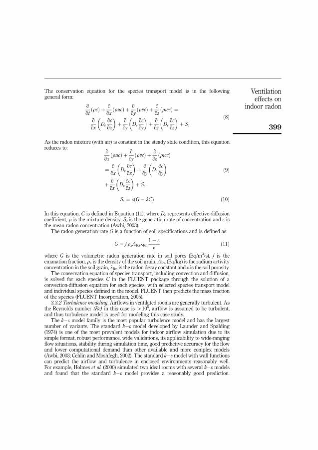
The conservation equation for the species transport model is in the followinggeneral form:
qqt
ðrcÞ þ qqx
ðrucÞ þ qqy
ðrvcÞ þ qqz
ðrwcÞ ¼qqx
Deqcqx
� �þ qqy
Deqcqy
� �þ qqz
Deqcqz
� �þ Sc
ð8Þ
As the radon mixture (with air) is constant in the steady state condition, this equationreduces to:
qqx
ðrucÞ þ qqy
ðrvcÞ þ qqz
ðrwcÞ
¼ qqx
Deqcqx
� �þ qqy
Deqcqy
� �
þ qqz
Deqcqz
� �þ Sc
ð9Þ
Sc ¼ eðG� lCÞ ð10Þ
In this equation, G is defined in Equation (11), where De represents effective diffusioncoefficient, r is the mixture density, Sc is the generation rate of concentration and c isthe mean radon concentration (Awbi, 2003).
The radon generation rate G is a function of soil specifications and is defined as:
G ¼ frsARalRn1� ee
ð11Þ
where G is the volumetric radon generation rate in soil pores (Bq/m3/s), f is theemanation fraction, rs is the density of the soil grain,ARa (Bq/kg) is the radium activityconcentration in the soil grain, lRn is the radon decay constant and e is the soil porosity.
The conservation equation of species transport, including convection and diffusion,is solved for each species C in the FLUENT package through the solution of aconvection-diffusion equation for each species, with selected species transport modeland individual species defined in the model. FLUENT then predicts the mass fractionof the species (FLUENT Incorporation, 2005).
3.3.2 Turbulence modeling. Airflows in ventilated rooms are generally turbulent. Asthe Reynolds number (Re) in this case is 4105, airflow is assumed to be turbulent,and thus turbulence model is used for modeling this case study.
The k�e model family is the most popular turbulence model and has the largestnumber of variants. The standard k�e model developed by Launder and Spalding(1974) is one of the most prevalent models for indoor airflow simulation due to itssimple format, robust performance, wide validations, its applicability to wide-rangingflow situations, stability during simulation time, good predictive accuracy for the flowand lower computational demand than other available and more complex models(Awbi, 2003; Cehlin and Moshfegh, 2002). The standard k�emodel with wall functionscan predict the airflow and turbulence in enclosed environments reasonably well.For example, Holmes et al. (2000) simulated two ideal rooms with several k�e modelsand found that the standard k�e model provides a reasonably good prediction.
399
Ventilationeffects on
indoor radon

Gadgil et al. (2003) also verified that the k�e model predicted the indoor-pollutantmixing time in an isothermal closed room fairly well. Zhang and Chen (2006)successfully applied the standard k�e model to predict the airflow and particledistribution in a room with an underfloor air distribution system.
Two-equation models are the simplest available means of calculating turbulentstresses in the recirculation flow where the length scale distribution cannot becalculated algebraically. As a two-equation model, the standard k�e model is a semi-empirical model based on model transport equations for the kinetic energy k and itsdissipation rate e. When using this model it is assumed that the flow is fully turbulentand that the effects of molecular viscosity are negligible (Awbi, 2003).
In this work we have used standard k�e model for numerical simulation of airflowin rooms.
3.3.3 Values and constants. Tables II and III show the values and constants used inthis study, which are used to indicate parametric values of variables in FLUENT.
3.3.4 Boundary conditions. Table IV indicates the boundaries in the model, theirlocations and physical descriptions. The last column also lists the boundary conditionoptions available in FLUENT.
At the minimum indoor air speed (0.5m/s), the Reynolds number reaches thetransition values and the flow becomes turbulent. The k�e model is therefore used tosimulate the turbulence.
3.3.5 Simulation procedure. In order to model the soil and house, three individualcases are defined to solve the governing equations. The simulation approach isrepeated for these three cases to show the influences of changing ventilation rates andinlet and outlet locations.
The initial condition is applied to the temperature field to calculate the buoyancyeffect of the flow and the disturbance pressure in the second run. The radonconcentration in the case study house before remedial techniques were applied, wasabout 4,000 Bq/m3, equivalent to just 5.25� 10�16 kg/m3.
Radon properties Usage Quantity
CP (J/kgK) Energy equation 96.35K (W/mK) Energy equation 0.00361MW (kg/kmol) Transport equation 222Density (kg/m3) Transport equation 7.13
Table II.Radon properties
Variable Quantity
Atmosphere pressure gage 0 PaAir leakage from door 0-0.2m/sAir leakage from window 0-0.02m/sIntake fan-pressure jump 0-20 PaExhaust fan-pressure jump �20-0 PaRadon source term 2.6e-17 kg/m3/sPermeability of soil 10-10m2
Porosity 0.4
Table III.Constants used inboundary conditions
400
MEQ24,3

3.3.6 Solution methods. The finite volume solution method can be used forsolving governing equations. This method either uses a “segregated” or a “coupled”solution procedure.
With segregated methods an equation for a certain variable is solved for all cells,and then the equation for the next variable is solved for all cells, etc.
With coupled methods, for a given cell equations for all variables are solved, andthat process is then repeated for all cells.
The segregated solutionmethod is the default method in most commercial finite volumecodes. It is best suited for incompressible flows or compressible flows at lowMach number.
Compressible flows at high Mach number, especially when they involve shockwaves, are best solved with the coupled solver.
3.3.7 Grid refinement. Grid refinement is deemed necessary when thesimulation grid cannot resolve the attributes accurately and is applied to minimizethe numerical diffusion.
Grid refinement should be continued until the solution is reasonably gridindependent. In order to achieve grid independency two aspects must be considered:grid distribution, and the total number of grid cells in the computational domain.
An acceptable grid with reasonable respect and aspect ratios results in fastconvergence, and residual errors decrease with increasing cell number. However,increasing grid refinement usually creates greater demands on computing capacityand cost (Wang and Ward, 2000).
The independency of grids was checked by increasing the mesh size by six steps,and results of finer grids were approximately equal. Some of the grid systems testedand the numbers of cells in them are shown in Table V.
The computational load increased rapidly after step 4, which contained 40� 32� 10cells. This step was therefore used in all simulation modeling. A further reason forselecting step 4 was that 3D modeling generally requires many more calculations, asthe parametric studies require a wide range of conditions in combination.
Location Physical description Option in FLUENT
Door Mass and heat leakage Velocity inletExhaust fan Pressure jump, no radon entry Exhaust fanFloor No-flow and vertical radon diffusion only InteriorIntake fan Pressure jump, no radon entry Intake fan
Roof No-flow boundary (including soil gas, radon) WallRoom walls No-flow boundary (including soil gas, radon) WallSoil bottom Fixed temperature; no-flow WallSoil surface Fixed temperature; fixed concentration; fixed pressure Pressure inletSoil wall No-flow boundary (including soil gas, radon and heat flux¼ 0) SymmetryWindow Mass and heat leakage Velocity inlet
Table IV.Boundary conditions
of the model
Grid 4 Grid 5
House 40� 32� 10 80� 64� 20Soil 120� 120� 12 120� 120� 12Total cells 185,600 275,200
Table V.Various grid systems
of 3D models
401
Ventilationeffects on
indoor radon

Larger numbers of grid cells were sometimes used to increase the accuracy of theresults. Thus, grid density was maximized based on accuracy and affordability.
4. Results and discussionAir conditioning in houses and living areas is an important consideration for design,operation and maintenance services. Study of its effect on radon distribution in house istherefore also important. However, its complexity limits the methods which can beused to study it. In this study we considered a simple and popular method of airconditioning and studied its behavior and effects on radon concentration. Fan-coils orfans are the most widely used class of air conditioning systems globally.
In this study we considered three intake fans and three exhaust fans in the room andset for them the conditions of fan-coils.
4.1 Exhaust fanThe figures below show the flow field in a house for a case study of an exhaust fan.In this case the pressure jump across the exhaust fan is set to 10 Pa. These figuresclearly illustrate the mixing behavior in the house for this condition. The indoor airvelocity and temperature are in the thermal comfort zone.
Figure 2 shows the velocity at the midpoint of the house in the case study for anexhaust fan with a pressure jump of 10 Pa.
Figures 3 and 4 show the variation of radon concentration in the house due to theeffect of the exhaust fan pressure jump. Increasing the pressure jump in the fan, resultsin lower radon concentration. This is because the larger pressure jump and mass flowrate, force the radon out of the room and decreases radon level at indoor environment.
2
Z X Y
Z
2.579612.235661.891711.547761.203820.8598690.5159210.171974
1
0–4
–2
Y 0
24
42
0X
–2
Figure 2.Velocity contours for twoperpendicular planescrossing the midpoint ofthe house in the case studyfor the exhaust fan with apressure jump of 10 Pafrom CFD model outputs
Radom distribution (Bq/m3) for X-plane 2.5
2
1.5
Z (m
)
1
0.5
0–4 –3
50 100 150 200 250
–2 –1 0Y (m)
1 2 3 4
Figure 3.Radon concentration at themidpoint of the house inthe case study for theexhaust fan with apressure jump of 10 Pafrom CFD model outputs
402
MEQ24,3

4.2 Intake fanIn some houses, air conditioning is performed with inlet fans instead of exhaust fans.In this part of the study we considered a house with three intake fans. The pressurejump across the fans was between 2 and 20 Pa. The contours below investigate the flowfield (air) properties throughout the house. The velocity and radon distribution areshown in Figures 5 and 6.
4.3 DoorsFigures 5 and 6 show that, the intake fans force air into the house causing the pressureinside to rise. Every house has doors and windows. Their effect is considered in airconditioning calculations for design and operation. Doors and windows result in
Radon concentration vs pressure jump in exhaust fan300
Rad
on (B
q/m
3 ) 250
200
150
100
50
00 2 4 6
Pressure jump in exhaust fan (pa)8 10 12 14 16 18 20
Figure 4.Radon concentration inthe house vs pressure
jump in the exhaust fanfrom CFD model outputs
2.5Radon distribution (Bq/m3) for X-plane
2
1.5
1
0.5
Z (m
)
0–4 –3 –2
Y (m)–1 0 1 2 3 4
50 100 150 200 250 300 350 400
Figure 6.Radon concentration at themidpoint of the house in
the case study for theintake fan with a pressurejump of 10 Pa from CFD
model outputs
2
X Y
Z
1
0–4
1.840391.5951.349620.104230.8588480.6134630.3680780.122693
–2–2
–4
0Y
0X2
2
4 4
N
Figure 5.Velocity contours for two
perpendicular planescrossing the midpoint of
the house in the case studyfor the intake fan with apressure jump of 10 Pa
from CFD model outputs
403
Ventilationeffects on
indoor radon

leakage of mass or heat or both. In this part of the study we examined the effect ofdoors on radon concentration and distribution in the house.
Figure 7 shows the effect of door leakage velocity on radon concentration inthe house. Increasing the velocity or mass flow rate leaking through the doordecreases the radon content of the house. The main reason for this is likely to be theincrease in internal pressure in the house and therefore door effect will be like anintake fan. Increasing internal pressure has two effects. One, takes the radon out ofthe house by increasing leakage velocity. Two, decrease the difference pressurebetween indoor and outdoor environment, driving force, which decreases radon entryrate into the house.
The heating, ventilation and air conditioning systems, because of the changingpressure or temperature, create pressure-driven convective flow, in which the apparentvelocity of fluid flow through a cross-sectional area is related to the pressure gradient(Spoel, 1998).
4.4 Analytical and measurements methods resultsIn this work an analytical solution and a measurement method have been used forvalidation of the numerical model. Each pressure jump in an intake fan or exhaust fancorresponds to a specific mass flow rate. In other words, different pressure jumpscorrespond to different ventilation rates. Here we have considered three air changerates for validation of the numerical model. Table VI shows the radon concentrations ofthe house from measurements, analytical calculation and numerical simulationtechniques. Comparison of these analytical data with the measured data showed closeagreement. This close agreement remained in spite of the errors inherent in all thetechniques, such as the 10 percent uncertainty in measurement by the CRM. Resultsshow that differences between analytical solution and numerical model are below 10percent (Table VI).
Results of measurement method have also been plotted in Figure 8 which ismeasured with a CRM.
160Radon concentration vs air velocity leaking door
140120
80
Rad
on (B
q/m
3 )
100
604020
00 0.02 0.04 0.06 0.08
Velocity of leakage (m/s)0.1 0.12 0.14 0.16 0.18 0.2
Figure 7.Effect of air velocityleakage through the dooron radon concentrationfrom CFD model outputs
Ach (h�1) Measurement (Bq/m3) Analytical (Bq/m3) Numerical (Bq/m3) Difference (%)
0.25 90 106 100 0.90.5 45 53 65 3.61 25 22 30 10.0
Table VI.Indoor radonconcentrations results
404
MEQ24,3

This analytical solution along measurement method gives sufficient validationfor the numerical model.
Results of the numerical study indicated that indoor pressure created by ventilationsystems and infiltration through doors or windows has significant effects on indoorradon content. Comparison of Figures 3 and 6 shows that the location of vents canaffect on indoor radon distribution and indoor radon level.
5. ConclusionsThe method by which radon concentration is modeled in FLUENT software is a keyfactor for solving transports equations in turbulence modeling and enhancingaccuracy of the results.
A model for radon entry through soil into a one family house in 3D was developedin FLUENT. The results indicate that indoor radon concentrations are dependent onventilation specifications and indoor and outdoor conditions.
Verification of the model and its performance show that radon entry to the houseand ventilation effects were well defined both physically and numerically.
The performance and sensitivity of the model were confirmed by changinga number of input parameters and boundary conditions.
According to the simulation results, distribution of radon is homogeneous exceptnear exhaust or intake fans. The concentration of radon decreases exponentially withincreasing indoor pressure and ventilation rate. The results of simulation, analyticalanalysis and measurement agreed well with each other.
Discrepancies found here between CFD simulation, measurement and mathematicalmethods may have resulted from insufficiently detailed representations of boundaryand initial conditions. It may be possible to further improve CFD results by using amore refined representation of grids and certain boundary conditions, such as pressureand temperature differences between the inside and outside. Meanwhile, the use of CFDfor quantitative estimation of indoor radon concentration requires careful validationof the CFD methods.
In conclusion, CFD is a powerful tool for exploring the factors that influenceradon distribution in residential buildings. However, the accuracy of simulations ofindoor radon and indoor conditions can only be confirmed for conditions that havebeen validated. This model may also be improved by considering some real situationsin residential buildings, internal heating sources and external situations. The problemcan be modeled by integration of all or specific combinations of parameters such as theoutdoor weather or indoor conditions.
20
29/04 18 30/04 00 30/04 06 30/04 12Time
30/04 18 01/05 00 01/05 06
3040506070
Bq/
m3 80
90100
0.5 Ach0.25 Ach
0.1 Ach110120
Figure 8.Radon level vs ventilation
rate from measurement
405
Ventilationeffects on
indoor radon
References
Ahmed, J.U. (1994), “Radon in the human environment: assessing the picture”, InternationalAtomic Energy Agency Bulletin, Vol. 36 No. 2, pp. 32-35.
Amissah, P.K. (2005), “Indoor air quality: combining air humidity with construction moisture”,working paper, Energy Systems and Research Unit, University of Strathclyde, Glasgow.
Arvela, H. (1995), Residential Radon in Finland: Sources, Variation, Modelling and DoseComparisons, Finnish Center for Radiation and Nuclear Safety, Helsinki.
Awbi, H.B. (2003), Ventilation of Buildings, Taylor & Francis, London.
Cehlin, M. and Moshfegh, B. (2002), “Numerical and experimental investigation of air flowsand temperature patterns of a low velocity diffuser”, Indoor air 2002 Proceedings of9th International Conference on Indoor Air Quality and Climate in Monterey, USA,Fraunhofer-Stuttgart, pp. 765-770.
Clavensjo, B. and Akerblom, G. (1994), The Radon Book: Measures Against Radon, The SwedishCouncil for Building Research, Stockholm.
Cohilis, P., Wouters, P. and L’Heureux, D. (1991), “Prediction of the performance of variousstrategies of subfloor ventilation as remedial action for radon problems”, VentilationSystem Performance Proceedings of AIVC 11th Conference, Belgirate, 1990, Vol. 2,pp. 17-40.
European Collaborative Action (2003), “Ventilation, good indoor air quality and rational use ofenergy”, working paper (Report No. 23, EUR 20741 EN), Office of Official Publications ofthe European Communities, Luxembourg.
FLUENT Incorporation (2005), FLUENT User’s Guide Version 6.3, FLUENT Inc, Lebanon, NH.
Gadgil, A.J., Lobscheid, C., Abadie, M.O. and Finlayson, E.U. (2003), “Indoor pollutant mixingtime in an isothermal closed room: an investigation using CFD”, AtmosphericEnvironment, Vol. 37 Nos 39-40, pp. 5577-5586.
Holmes, S.A., Jouvray, A. and Tucker, P.G. (2000), “An assessment of a range of turbulencemodels when predicting room ventilation”, Healthy Buildings 2000 Proceedings of theInternational Conference in Espoo, Vol. 2, pp. 401-406.
Kokotti, H. (1995), Dependence of Radon Level on Ventilation Systems in Residences, KuopioUniversity Publication, Kuopio.
Launder, B.E. and Spalding, D.B. (1974), “The numerical computation of turbulent flows”,Computer Methods in Applied Mechanics and Engineering, Vol. 3 No. 2, pp. 269-289.
Loureiro, C.O. (1987), Simulation of the Steady-State Transport of Radon from Soil into Houseswith Basements under Constant Negative Pressure, Lawrence Berkeley NationalLaboratory, University of California, Berkeley, CA.
Man, C.K. and Yeung, H.S. (1997), “The effects of cracks and holes on the exhalation of radonfrom concrete”, Building and Environment, Vol. 32 No. 4, pp. 351-354.
Marley, F. and Phillips, P.S. (2001), “Air-movement control of radon in a retail store”,Environmental Management and Health, Vol. 12 No. 5, pp. 483-491.
Mora, L., Gadgil, A.J. and Wurtz, E. (2003), “Comparing zonal and CFD model predictions ofisothermal indoor airflows to experimental data”, Indoor Air, Vol. 13 No. 2, pp. 77-85.
Nilsson, P.E. (2003), Achieving the Desired Indoor Climate: Energy Efficiency Aspects of SystemDesign, Studentlitteratur AB, Lund.
Petropoulos, N.P., Anagnostakis, M.J. and Simopoulos, S.E. (2001), “Building materials radonexhalation rate: ERRICCA intercomparison exercise results”, Science of The TotalEnvironment, Vol. 272 Nos 1-3, pp. 109-118.
Pitarma, R.A., Ramos, J.E., Ferreira, M.E. and Carvalho, M.G. (2004), “Computation fluiddynamics: an advanced active tool in environmental management and education”,
406
MEQ24,3
Management of Environmental Quality: An international Journal, Vol. 15 No. 2,pp. 102-110.
Radonelektronik (2012), “Electronic Radon Gas Monitor”, available at: www.radonelektronik.se(accessed July 13, 2012).
Rota, R., Canu, P., Carra, S. and Nano, G. (1994), “Ventilated enclosure with obstacles:experiments and CFD simulations”, Ventilation for Contaminant Control Proceedings ofthe 4th International Symposium in Cincinnati, OH, Vol. 1, pp. 181-186.
Spoel, W.H. (1998), “Radon transport in sand: a laboratory study”, working paper, TechnischeUniversiteit Eindhoven, Eindhoven, March 23.
Tung, T.C.W. and Burnett, J. (2004), “Radon measurement protocol for residences with differentventilation rates”, Indoor and Built Environment, Vol. 13 No. 2, pp. 133-138.
Wang, F. and Ward, I.C. (2000), “The development of a radon entry model for a house with acellar”, Building and Environment, Vol. 35 No. 7, pp. 615-631.
Zhang, Y. (2004), Indoor Air Quality Engineering, CRC Press, Boca Raton, FL.
Zhang, Z. and Chen, Q. (2006), “Experimental measurements and numerical simulationsof particle transport and distribution in ventilated rooms”, Atmospheric Environment, Vol.40 No. 18, pp. 3396-3408.
Zhou, W., Iida, T., Moriizumi, J., Aoyagi, T. and Takahashi, I. (2001), “Simulation of theconcentrations and distributions of indoor radon and thoron”, Radiation ProtectionDosimetry, Vol. 93 No. 4, pp. 357-367.
About the authors
Keramatollah Akbari is a PHD student at the Malardalen University, Sweden. He is also anacademic member at ACECR – Fars Branch and trainer of Entrepreneurship in Shiraz University,Iran. He teaches such courses as General Mathematics, Statistics & Probability, SystemsAnalysis and Design, Management Principles and Entrepreneurship. He is also involved in theprojects of radon reduction and energy consumption in buildings, priorities in electronicindustries units, project considering the establishment of aggregation, processing and marketinginformation center, considering new job opportunities in the field of information technology (IT)and electronics, business plan of civil information and services center.
Jafar Mahmoudi is an Adjunct Professor at the Malardalen University, Department of PublicTechnology, Energy Tech, Vasteras, Sweden. His university chair is Process Optimization inMetal Industry. He is the head of directing board and president of MESET, Sweden. His majorresearch focus is development of new technology and methods for industrial energy optimizationwith special focus on heat and mass transfer. He has years of theoretical and experimentalexperience on this. He also has a broad technical background encompassing thermodynamic,numerical methods and modeling (CFD computation), as well as materials science.
Mahdi Ghanbari graduated as Master of Science in Energy Systems Engineering in 2009.The studies were conducted at the Department of Energy Engineering at the Sharif Universityof Technology, Iran. He is now working on the projects at the ACECR – Sharif University Branch,primarily with computational fluid dynamics within a wide range of applications.He is also involved in the projects of energy auditing in industries and projects including CHPsystems design, heat exchangers design, optimization using genetic algorithm and energyrecovery systems.
To purchase reprints of this article please e-mail: [email protected] visit our web site for further details: www.emeraldinsight.com/reprints
407
Ventilationeffects on
indoor radon

Paper III

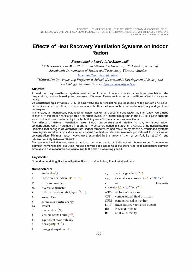
PROCEEDINGS OF ECOS 2012 - THE 25TH INTERNATIONAL CONFERENCE ON EFFICIENCY, COST, OPTIMIZATION, SIMULATION AND ENVIRONMENTAL IMPACT OF ENERGY SYSTEMS
JUNE 26-29, 2012, PERUGIA, ITALY
329-1
Effects of Heat Recovery Ventilation Systems on Indoor Radon
Keramatollah Akbaria, Jafar Mahmoudib aTDI researcher at ACECR, Iran and Mälardalen University, PhD student, School of
Sustainable Development of Society and Technology, Västeras, Sweden [email protected]
bMälardalen University, Adj Professor at School of Sustainable Development of Society and Technology, Västeras, Sweden [email protected]
Abstract A heat recovery ventilation system enables us to control indoor conditions such as ventilation rate, temperature, relative humidity and pressure difference. These environmental conditions affect indoor radon levels. Computational fluid dynamics (CFD) is a powerful tool for predicting and visualizing radon content and indoor air quality and is cost effective in comparison with other methods such as full scale laboratory and gas trace techniques. In this study a mechanically balanced ventilation system and a continuous radon monitor (CRM) were used to measure the indoor ventilation rate and radon levels. In a numerical approach the FLUENT CFD package was used to simulate radon entry into the building and effects on indoor air conditions. The effects of different ventilation rates, indoor temperature and relative humidity on indoor radon concentrations were investigated in a one family detached house in Stockholm. Results of numerical studies indicated that changes of ventilation rate, indoor temperature and moisture by means of ventilation systems have significant effects on indoor radon content. Ventilation rate was inversely proportional to indoor radon concentration. Minimum radon levels were estimated in the range of thermal comfort, i.e. at 21 and relative humidity between 50-70%. The analytical solution was used to validate numeric results at 3 distinct air change rates. Comparisons between numerical and analytical results showed good agreement but there was poor agreement between simulations and measurement results due to the short measuring period. Keywords: Numerical modeling, Radon mitigation, Balanced Ventilation, Residential buildings Nomenclature A surface
radon concentration
diffusion coefficient Dh hydraulic diameter
radon exhalation rate
source term K turbulence kinetic energy Pa Pascal T temperature ( )
volume of the house Ur equivalent room velocity
density
energy dissipation rate
air change rate
radon decay constant
ν air kinematic viscosity
ATD alpha track detector CFD computational fluid dynamics CRM continuous radon monitor HRV heat recovery ventilation system Re Reynolds number RH relative humidity

329-2
1.Introduction
Understanding indoor radon transport and distribution is a priority, and for this it is important to be able to predict indoor air quality and the exact value of radon level at different points and areas, especially in breathing zones in residential buildings. Indoor radon distribution and treatments have been studied through measurements and full scale laboratory and tracer gas models. These methods are rather expensive and time consuming. Analytical methods are also limited to varying ventilation rates, and radon measurements are generally expressed as average monthly or annual levels. A numerical modeling approach using computational fluid dynamics (CFD) techniques may be a powerful and cost-effective tool to study and predict indoor radon distribution. Numerical models can be used to estimate the importance of specific factors for radon entry. These models also can provide a cost-effective test bench for improved designs of radon prevention systems [1,2]. CFD techniques are based on solving the transport equations iteratively and are employed to solve equations involving velocity, temperature and species transport numerically in a finite volume. They describe the processes in the ventilated room, including the conservation of mass, energy, momentum and species such as radon [3, 4]. Numerous studies have used CFD to study the distribution of indoor air flow and radon concentration in two and three dimensions. Some of these studies are described in the following paragraphs. Zhuo [5] used CFD to study the concentrations and distributions of indoor radon in three dimensions. According to the results of this simulation, the distribution of radon in a ventilated room is uniform except at locations near air diffuser vents. He showed that the results of simulations of activities and their distributions agreed well with experimental results in a laboratory. Feng and Persily [6] performed computer simulations of airflow and radon transport in a large building using the multi-zone airflow and pollutant transport model CONTAM88. This study investigated ventilation system factors including the operation of exhaust fans and variations in outdoor air intake. Wang and Ward [7] used the CFD package FLUENT to develop a model of multiple radon entry in a house with a cellar. In o rde r to develop the model, they applied methods such as using a subroutine to specify the radon generation rate in the soil cells and designed appropriate boundary conditions. The model was verified by a grid-independency test and convergence behavior analysis. The inter-model validation technique and comparison with analytical solutions were also used to validate the model. Cohilis [ 8 ] suggested the use of a numerical code based on the finite difference method. Based on the results and the code validation, they concluded that this method was a powerful tool that could predict and evaluate the performance of subfloor ventilation strategies. Rota [9] compared the results of numerical simulations and experiments. The results showed good agreement, but the simulation results showed elevated concentrations in the region with low ventilation rates compared to the experiments. Unlike the previous cited works, this study focuses on indoor radon concentration, in this case the diffusion and advection forces are considered and there is not any radon decay and generation rate.
1. Material and Methods

329-3
In this study a continuous radon monitor (CRM) and alpha track detectors (ATD) were used to measure indoor radon concentrations. A one family detached house with a rotary heat exchanger ventilation system was used in a case study. Numerical methods, measurement and analytical calculations were used to estimate radon levels, as detailed in the following section. The house consists of eight rooms with a total volume of 12×9×2.4 m3. Each room has its own vent except for Room 8, which shares a vent with Room 6. All doors are kept open. A rotary heat exchanger is placed in Room 4. The effect of the heat exchanger is ignored and an outlet vent is considered in Room 4 to play the role of the heat exchanger. Figure 1 shows the geometry of the house plan. 2.1. Numerical method In the numerical approach the commercial CFD package including GAMBIT was used to define the geometry, and FLUENT 6.3 [10] was used as the solver for calculations to simulate radon entry into the building and ventilation effects. The selected 3dimentional model was: species transport, pressure base and steady state, k–ε turbulence, and the SIMPLE algorithm were used to calculate and predict radon concentration at all grid locations numerically.
Fig.1. The geometry of the house plan
The model is meshed with 376238 hexahedral cells with 10 cm vertices in order to solve the conservation equations of various fluid properties within each cell. These equations are flow, energy, turbulence, radon and humidity. Three criteria were considered to confirm the model convergence. The first criterion was the residuals of equations residuals could not change drastically through iterations and the residuals of all the conservation equations had to be less than 1 × 10⁻⁷. The second criterion was that the concentration of radon in one of the rooms (Room 1) could not change through iterations. The third criterion concerned the rate of radon passing through the outlet. As the model is solved for the steady state, all radon which is generated in the floor must also pass through the outlet, i.e. radon rate from the outlet must be equal to the radon generation rate. Specifically, radon rate through the outlet must be 2 bq/s and 3 bq/s for 1 Pa and 2 Pa pressure differences respectively. In order to avoid residual instability and oscillations, under relaxation factors were adjusted to speed up the convergence. The results of using 376238 and 752476 cells were compared to ensure that the grid cells were sufficiently small to ensure accurate results.

329-4
The model was solved for four different air change rates. Specifically, Ach=0.05, 0.25, 0.5 and 1.2. Temperature and relative humidity were assumed to be fixed at 30 °C and 30% respectively in these cases. The difference pressure was set at 1kPa.
2.1.1. Initial values and boundary conditions The materials used in the model are air, water vapor, radon as a fluid in a mixture and light concrete for the floor, dense concrete for walls, windows material and main door as solid materials. Internal doors are left open. Properties of radon are given in the previous sections. Properties of the other materials are as shown in Tables 1 and 2.
Table 1. Properties of Fluids Properties
Air Water Vapor
Radon
Density (kg/m3) 1.225 0.5542 9.73 Cp (j/kg-k) 1006.43 2014 96.35 K (w/m-k) 0.0242 0.026 0.0036 Viscosity(kg/m.s) 1.7894×10⁻⁵ 1.34×10⁻⁵ 1.8×10⁻⁵ MW (kg/kmol) 28.966 18.0153 222
Table 2. properties of Solids Material
Density kg/m3
Cp j/kg-k
K w/m-k
Light concrete 1200 1000 0.4
Dense concrete 2100 840 1.4
Windows 2700 880 0.8
Main Doors 720 1250 0.16
Boundary conditions in the model are: 7 vents in rooms, outer surfaces, floor zone, outlet, walls zones and room zones. Characteristics of these boundaries are as follows. The vent in each room is defined as the velocity inlet boundary. Specifications which must be defined for this type of boundary are velocity, hydraulic diameter, temperature and mass fraction of radon and mass fraction of water vapor.
2.2. Measuring method Radon concentrations were measured continuously during winter and spring, both with a continuous radon meter (CRM) and an alpha track detector (ATD). The air change rates in the house also were measured by the heat recovery ventilation (HRV) system.
2.3. Analytical method Indoor radon content can be calculated as
(1)

329-5
Where is indoor radon concentration at the steady state, is radon
exhalation rate, is the radon exhalation surface (in this study the house floor), is the
volume of the house, is the radon decay constant and is the air change
rate in the house and h=2.4 m is the height of the house. For (11) and the given data of the case study house, Equation (1) gives indoor
radon levels for different ventilation rates (0, 0.25, 0.5 and 1).
3. Results and discussion
3.1. Numerical results
Graphical presentations of the three dimensional simulation data were prepared using FLUENT contours. These contours are a good tool for qualitative comparisons. From the FLUENT report, it is also possible to determine the numeric data for quantitative comparisons. This study investigated the effects of: 1. Ventilation rate, 2. Temperature, 3. Relative humidity, and 4. Pressure difference 1.Ventilation rate: Contours of radon concentration in the house plan at position y=210 cm from the floor for various air change rates are shown in Figure 4. This figure shows qualitative comparisons of radon concentrations at four different hourly air change rates ranging from 0.05 to 1.2 Ach. As evident from Figure 5, different ventilation rates have distinct effects on indoor concentration in Room 1. The quantitative comparisons are plotted in Figure 6, which shows that the radon concentration levels were inversely proportional to outdoor flow rate at steady state. Numerical simulations were performed at different Reynolds numbers. The Reynolds number in the house was calculated using Equation (2):
Figure 4. Contours of radon concentration in the house plan (Room1) with air change rates
0.05-1.2 Ach Re = Dh × Ur/ν (2)

329-6
where Dh is the hydraulic diameter of room and is defined as: 2WH/(W + H) (W = width, H = height), Ur is the equivalent room velocity (flow rate/cross-sectional area) and ν is the kinematic viscosity of air [3]. The Reynolds numbers were 2 × 10⁴ and greater than 2 × 10⁵, corresponding to ventilation rates of 0.05 and greater than 0.5 Ach.
Figure 5. Radon concentrations in Room1 versus air change rate
2. Temperature: In order to investigate the effects of temperature changes on radon concentration, air change and relative humidity were fixed and indoor temperature was varied between 15 °C to 25 °C. Air change and relative humidity were maintained at 0.5 and 30% respectively. The temperature effects are shown qualitatively in Figure 6. Indoor radon levels were inversely proportional to indoor temperature. This is because of the direct correlation between temperature and pressure as stated by the constant gas law. Thus, increasing temperature increases the pressure, and since the indoor radon concentration is driven by pressure, the amount of radon driven into the room decreases. From another perspective, increasing the house temperature increases indoor pressure and the outside acts a vacuum cleaner and sucks away the indoor air. This phenomenon is referred to as the "stack effect"[12].
Figure 6. Contours of radon concentration in Room 1 at different temperatures
Figure 7 shows the contours of radon concentration at y=120 cm from the floor for various temperatures.

329-7
Fig.7. Radon concentrations in Room1 versus temperature
3. Relative humidity The effect of varying relative humidity on radon concentration in Room 1 is shown in Figure 8. Relative humidity is varied between 30 to 80% and temperature and air change are maintained at 18ºC and 0.25 respectively. Figure 8 indicates that radon concentration decreases from RH 30% to 70%, and increases when RH rises from above 70%. This is because increasing humidity from zero to a defined quantity below 50% increases the pressure gradient in air. This increases the driving force that draws the radon out of the ground. However, higher RH levels result in denser air, and radon is unable to rise to high altitudes. Increased moisture in air also decreases diffusion coefficient and hence reduces the diffusion length of radon, which reduces transfer of radon to areas of low radon concentration.
Fig. 8. Radon concentrations in Room1 versus relative humidity
4. Pressure difference The model was solved for 1 Pa and 2 Pa difference pressures. Radon entry rate varies with pressure difference. Previous work in the field has established entry rates of 2 Bq/s and 3 Bq/s for pressure differences of 1 Pa and 2 Pa respectively [1]. Air change rate, temperature and relative humidity are maintained at 0.25, 18 ºC and 40% respectively. Contours of radon concentration in a plane at y=120 cm from the floor are shown in Figure 9, and clearly show that pressure difference affects indoor radon levels.

329-8
Figure 9. Contour of radon concentration for Δp=1Pa and 2 Pa
3.2 Measuring results The results of measurements are shown in Table 3. In order to show the impact of ventilation rate on radon level, radon concentrations were measured at three different ventilation rates. Figure 10 shows the results at three different air change rates, measured with a CRM. The figure shows that measured radon levels were inversely proportional to air exchange rate. Continuous radon measurements using a CRM also confirmed that in the indoor temperature range, fluctuating radon levels in the house have a strong indirect correlation with temperature (Figure 11).
Table 3. Measured indoor radon levels (Bq.m-3)
Date and period
ATD CRM Ventilation rate
Ventilation type
Remedial action
2008-2 (2weeks)
3580 380 ------ 0.25 Extract fan No action
2010-1 (3months)
1280 160 1580 158 0.25 HRV Radon sump &sealing
2010-04 (3 weeks)
100 20 ------ 0.5 HRV 3connected sumps
2010-3 (12days)
------- 97 10 0.5 HRV 3connected sumps
2010-3 (12days)
------- 65 6 0.5 HRV 3connected sumps
2010-4 (12 days)
------- 36 4 1 HRV 3connected sumps
Fig.10. Measured radon level measurements versus ventilation rate

329-9
3.3. Analytical results As previously mentioned, Equation (1) was used for analytical calculation and air change rates were set at 0.25, 0.5, and 1.2 h-1. The results are shown in Table 4.
4. Defined Functions In our estimates, radon concentrations are given in bq.m-3, whereas the FLUENT package gives molar concentration of radon in kmol.m-3. We therefore define a Custom Field Function to calculate radon concentration (bq.m-3) in term of molar radon concentration as follows:
(3)
Where = 222 is the molecular weight of radon.
Fig.11. Radon level (green) versus temperature (black)
5. Model Validation Model validation was performed using analytical solution. The numeric differences between numerical simulation and analytical calculation results are shown in Table 4. For quantitative comparisons, the percentage difference between the results of estimation by FLUENT and the analytical calculations were computed at each ventilation rate. The maximum difference was found to be below 10%. Measurement data were not suitable for comparison, because the measuring period was too short to obtain an acceptable average radon level.
Table 4.Indoor radon concentrations result in
Ach Measurement Analytic Numeric 0.0 3580 3582 ----- 0.25 90 106 107 0.5 45 53 55 1.2 25 22 20
6. Conclusion

329-10
The models were developed in FLUENT with simulated radon entry through the floor into a one family house in three dimensional models. The results support the hypothesis that indoor radon concentrations are indoor temperature and moisture dependent. The verification of the model and its performance indicate that radon entry to the house and the effects of temperature and moisture have been well defined physically and numerically. The performance and sensitivity of the model was confirmed by varying input parameters and boundary conditions. The effects of different parameters of indoor air such as ventilation rate, indoor-outdoor pressure difference, indoor temperature and relative humidity on indoor radon concentrations were investigated. The value of mass flow rate at the air inlet outlet affected the distribution patterns of indoor radon, both qualitatively and quantitatively. Discrepancies were found here between CFD simulation, numerical calculations and measurement data. These may have resulted from insufficiently detailed representation of boundary conditions and inaccuracies of measured data due to the short measurement period. In conclusion, CFD is a powerful research tool for predicting the factors that influence indoor radon distribution. However, further improvement of the accuracy of the quantitative estimations of radon concentration will require more detailed consideration of turbulence, near wall effects, grid refinement near the vents, and development of a robust validation method.
References [1] Andersen C. E., Numerical modeling of radon-222 entry into houses: an outline of techniques
and results, the science of total environment, 2001, Vols. 272: 33-42. [2] Wang F., Ward I. C., Radon entry, migration and reduction in houses with cellars, 2002, Vols.
37 (2002) 1153 – 1165. [3] Awbi H.B., Ventilation of building,. 2003. [4] Loureiro C.O., Simulation of the steady-state transport of radonfrom soil into houses with
basement under constant negativepressure. s.l. Report no. LBL-24378. Lawrence Berkeley Laboratory, Berkeley, CA., 1987.
[5] Zhuo W., Iida T., Moriizumi J., Aoyagi T. and Takahashi I., Simulation of the concentrations and distributions of indoor radon and thoron, 2000.
[6] Fang J. B., Persily A. K., Computer Simulations of Airflow and Radon Transport in Four Large Buildings, Building and Fire Research Laboratory, 1995.
[7] Wang F., and Ward I. C., Development of a radon entry model for a house with a cellar, 2000, Vols. 35 (2000) 615-631.
[8] Cohilis P., Wouters P., and L'Heureux D., Prediction of The Performance of Various Strategies of Subfloor Ventilation as Remedial Action For Radon Problems. 2004.
[9] Rota, R.,Ventilated enclosure with obstacles: experiments and CFD simulations. Cincinnati, OH: NIOH. pp. 181–6. : s.n., 1994. In Proceedings of the 4th International Symposium on Ventilation for Contaminant Control. Vol. 1.
[10] FLUENT Incorporated. FLUENT. User's Guide Version 6.3. Linux Format, Cavendish Court,Lebanon, NH 03766, USA: s.l. FLUENT, 2005. 2005.
[11] Goto M., Estimation of Global Radon Exhalation Rate Distribution. 2008. [12] Hoffmann R. L., Radon contamination of residential structure, an overview of factors
influence infiltration rates. s.l. Illinois Central College, 1997.

Paper IV


Author's personal copy
Influence of indoor air conditions on radon concentration in a detached house
Keramatollah Akbari a,b,*, Jafar Mahmoudi b, Mahdi Ghanbari c
aACECR, Fars Branch, Shiraz, IranbMälardalen University, School of Sustainable Development of Society and Technology, Box 724 80, Västeras, Swedenc Sharif University of Technology, Tehran, Iran
a r t i c l e i n f o
Article history:Received 11 February 2012Received in revised form28 July 2012Accepted 23 August 2012Available online
Keywords:Numerical modelingRadon mitigationAir change rateTemperatureRelative humidity
a b s t r a c t
Radon is released from soil and building materials and can accumulate in residential buildings. Breathingradon and radon progeny for extended periods hazardous to health and can lead to lung cancer. Indoorair conditions and ventilation systems strongly influence indoor radon concentrations. This paper focuseson effects of air change rate, indoor temperature and relative humidity on indoor radon concentrations ina one family detached house in Stockholm, Sweden.
In this study a heat recovery ventilation system unit was used to control the ventilation rate anda continuous radon monitor (CRM) was used to measure radon levels. FLUENT, a computational fluiddynamics (CFD) software package was used to simulate radon entry into the building and air change rate,indoor temperature and relative humidity effects using a numerical approach.
The results from analytical solution, measurements and numerical simulations showed that air changerate, indoor temperature and moisture had significant effects on indoor radon concentration. Increasingair change rate reduces radon level and for a specific air change rate (in this work Ach ¼ 0.5) there wasa range of temperature and relative humidity that minimized radon levels. In this case study minimumradon levels were obtained at temperatures between 20 and 22 �C and a relative humidity of 50e60%.
� 2012 Elsevier Ltd. All rights reserved.
1. Introduction
Indoor air change rate, temperature and relative humidity havesignificant effects on radon levels in residential buildings. Activeand appropriate ventilation can control the ventilation rate andmaintain indoor conditions in order tomitigate radon in residentialbuildings (Clever, 1979; Surbeck, 1996).
Numerous studies have found that indoor radon generallycorrelates with indoor and outdoor air conditions, and factors suchas indoor and outdoor pressure, temperature, moisture, ventilationrate and precipitation can affect radon entry into buildings(Andersen, 2001; Van der Pal and Van der Spoel, 2001). In thisstudy we focus on the effects of indoor air change rate, temperatureand relative humidity on indoor radon.
Computational fluid dynamics (CFD) is a powerful tool that cansimulate and predict airflow patterns, indoor air conditions andconcentration distributions of pollutants in a space at low cost. Inthis study, FLUENT, a CFD software package was used to simulate
and predict radon distribution and visualize the effects of indoor airtemperature and moisture. Analytical solution and measurementswere also performed for validation of numerical simulation.
2. Problem specifications
The case study is a one family detached house located inStockholm, built on bedrock in 1975. The house plan comprises of 8rooms and its volume is 12 � 9 � 2.4 m3. Each room has its ownvent, except Room 8, which shares a ventwith Room 6. All doors aresupposed to be kept open. A rotary heat exchanger is placed inRoom 4. Here the effect of the heat exchanger is ignored and anoutlet vent is considered instead to play the role of the heatexchanger in Room 4. The house is occupied but there is no energysource among furniture and they are not too large that can affect onradon concentration and distribution in the house. So we canneglect the effects of furniture in the model. Fig. 1 presents thehouse plan. The air change rate in each of the rooms corresponds tothe volume of that room, and all inlet air from the rooms passesthrough the unique outlet.
The radon level after some remediation was around 600 Bq/m3,mainly originating as soil gas from the building’s foundations. Thehouse is in direct contact with the ground, and radon entry is drivenby two disturbance pressures along its route into the house.
* Corresponding author. Mälardalen University, School of Sustainable Develop-ment of Society and Technology, Box 724 80, Västeras, Sweden.
E-mail addresses: [email protected] (K. Akbari), [email protected] (J. Mahmoudi), [email protected] (M. Ghanbari).
Contents lists available at SciVerse ScienceDirect
Journal of Environmental Radioactivity
journal homepage: www.elsevier .com/locate / jenvrad
0265-931X/$ e see front matter � 2012 Elsevier Ltd. All rights reserved.http://dx.doi.org/10.1016/j.jenvrad.2012.08.013
Journal of Environmental Radioactivity 116 (2013) 166e173

Author's personal copy
The research methods include analytical solution, measure-ments and numerical simulation.
Radon entry into a one family detached house and effects ofventilation rate, temperature and moisture are modeled using theFLUENT package in a three dimensional steady state model. Acontinuous radon monitor (CRM) was used to measure the indoorradon and check the numerical modeling method. Analyticalsolutionwas also performed for validating of numerical simulation.
3. Numerical simulation approach
FLUENT software can model the mixing and transport ofchemical species by solving conservation equations describingconvection and diffusion. For all flows, FLUENT solves conservationequations of mass and momentum. In this work, flows involve heatand species transfer, thus additional equations of energy andspecies conservation must be solved (FLUENT Incorporation, 2005).
In this study, a turbulent model is used, because airflow ina ventilated room even with ventilation rates below 0.2 m/s isusually in the turbulent regime, and the turbulent ke 3model isused to solve the governing equations (Wang andWard, 2000). Thestandard ke 3model is a popular method for numerical simulationof airflow in a room. In FLUENT we define the model as speciestransport with a mixture of air, radon and water vapor.
3.1. Determining flow pattern
Flowpattern can be determined bycalculating Reynolds number.Reynolds number can be obtained from the following expression:
Re ¼ VLn
(1)
Where, n is the kinetic viscosity of the mixture, V is the velocity ata vent and L is the characteristic length, for example the channelwidth (Andersen, 2001). Because there are several rooms andtherefore several vents, here we use the highest velocity to calcu-late the Reynolds number. The critical Reynolds number of 2000, atwhich transient flow becomes turbulent, is used to determine theflow pattern (Lesieur, 1990; Sun et al., 2002).
Re0:5 ¼ VLn
¼0:16389
ms� 0:3 m
1:115� 10�5 m2
s
¼ 4409:6>2000 ��!yieldsTurbulent flow
3.2. Radon transport equation
For the steady state condition and constant density of radon, thetransport equation is written as:
divðrCVÞ ¼ divðrD gradðCÞÞ þ S (2)
In the above expression, C is the radon concentration, S is thesource term and V is the velocity vector, r is the density of the radonand D is the diffusion coefficient (Surbeck, 1996). As radon istransported to the air and there is no radon generation and decay inthe air itself, S¼ 0, and Equation (2) reduces to Equation (3) in threedimensions. FLUENT solves this equation using numerical methods.
vðCuÞvx
þ vðCvÞvy
þ vðCwÞvz
¼ v
vx
�DvCvx
�þ v
vy
�DvCvy
�þ v
vz
�DvCvz
�
(3)
This equation calculates the radon content at any point in thehouse.
3.3. Temperature and relative humidity effects on radon properties
Some radon properties, such as radon diffusion coefficient,radon emanation coefficient and radon exhalation rate correlatewith temperature, relative humidity and pressure field.
The radon emanation factor is moisture dependent and reachesa constantmaximumvalue asmoisture content increases to between0.1 and 0.5. Since radon exhalation rate is a function of radonemanation coefficient, radon exhalation rate is also moisturedependent.
The radon exhalation rate increases with temperature, but thiseffect is smaller than the effect of moisture (Stranden et al., 1984).
Nomenclature
k Kinetic energyCp Specific heat (J/kg K)n Kinetic viscosity (kg/m s)u,v,w Velocity components in x, y, and z e coordinatesA Area (m2)MW Molecular weight (kg/k mol)RH Relative humidityC Radon concentration (Bq/m3)L Characteristic length (m)Ach Air changeCRM Continuous radon monitor
Grad GradientK Thermal conductivity (W/m K)3 Dissipation rateS Source termV Velocity vector (m/s)r Density (kg/m3)D Radon diffusion coefficient (m2/s)T Temperature (�C)Dp Pressure difference (Pa)V Velocity (m/s), Volume (m3)Re Reynolds numberCFD Computational fluid dynamicsDiv Divergence
Fig. 1. The geometry of the house plan.
K. Akbari et al. / Journal of Environmental Radioactivity 116 (2013) 166e173 167

Author's personal copy
The radon diffusion coefficient in air and water are1.1 �10�5 m2s and 1.2 � 10�9 m2s respectively. The radon diffusioncoefficient in water is thus much smaller than in air.
The relationship between temperature and radon diffusioncoefficient is shown in Equation (4). This equation shows thatincreasing temperature increases radon diffusion coefficient.
D ¼ D0e�QRT (4)
Where:
D0 ¼ Open air radon diffusivity in m2/sQ ¼ Activation energy in J mol�1
R ¼ Gas constant 8.31 J mol�1 K�1
T ¼ Temperature in Kelvin
The dependence of the diffusion coefficient on the relativehumidity was reported by Kotrappa et al. (1976), who showed thatthe maximum value of the diffusion coefficient occurs at 20e80%relative humidity.
Humidity is the amount of water vapor or moisture containedwithin the air. Relative humidity is defined as:
Relative humidity ðRHÞ ¼ PactualPWater
� 100% (5)
Where:
Pactual ¼ Actual partial vapor pressurePwater ¼ Saturation vapor pressure of water
The saturation vapor pressure of water (Pwater) can be expressedas (Sonntag, 1990):
Pwater ¼ ae
�bTcþT
�(6)
where, a, b and c are constants; a ¼ 6.112, b ¼ 17.62 and c ¼ 243.12and �45 < T < 50 �C.
This equation demonstrates the effect of temperature on satu-ration vapor pressure of water. The balance between the conden-sation and evaporation of water leads to vapor pressure, whichdepends on the temperature. Air can hold more vapor at hightemperatures than at low temperatures.
The total pressure of air (P) is related to Pwater and defined asfollows:
P ¼ Pdry air þ Pwater (7)
Where:
P ¼ Pressure disturbance field (relative to absolute pressure)(Pa)
On the other hand, P and V have a direct correlation. As in theradon transport equation (Equation (2)), the term V is pressure fielddependent because of the advection mechanismðVVC ¼ �k=mVPVCÞ of the indoor radon transport.
This relation indicates that relative humidity due to changingthe total pressure has an influence on indoor radon concentration.
3.4. Model meshing
Themodel is meshedwith 10 cm hexahedral elements. All stateswere solved with this mesh. In order to perform a grid
independency check in the later sections, a second mesh wasconstructed for the model (see Fig. 2).
3.5. Materials
The materials considered in the model are air, water vapor,radon, light concrete for the floor, dense concrete for walls,windows material and main door material. Internal doors aresupposed to be open. Properties of materials are shown in Table 1.
3.6. Boundary conditions
Boundary conditions in the model are: 7 vents in rooms, outersurfaces, floor zone, outlet, walls zones and rooms zones. Charac-teristics of these boundaries are as follows:
The vent in each room is defined as the velocity inlet boundary.Specifications that must be defined for this type of boundary arevelocity, hydraulic diameter, temperature, mass fraction of radonand mass fraction of water vapor.
Each room has the same type of vent, each with an area of0.06 m2. Velocity can be obtained from the following expression.
V ¼ Ach� VolumeRoomAreaVent
(8)
Forexample forRoom1andthe followingspecification:Ach¼0.5,VRoom 1 ¼70.8 m3, T ¼ 21 �C, RH ¼ 30, Dp ¼ 1 Pa, Turbulent flow
V ¼ Ach� VolumeRoomAreaVent
¼0:5
1h� 70:8 m3 � 1 h
3600 s0:06 m2
¼ 0:16389ms
3.7. Solution methods
The finite volume solution method can be used for solvinggoverning equations. This method either uses a “segregated” ora “coupled” solution procedure.
With segregated methods an equation for a certain variable issolved for all cells, and then the equation for the next variable issolved for all cells, etc.
With coupledmethods, for a given cell equations for all variablesare solved, and that process is then repeated for all cells.
Fig. 2. Top view of the meshed model.
K. Akbari et al. / Journal of Environmental Radioactivity 116 (2013) 166e173168
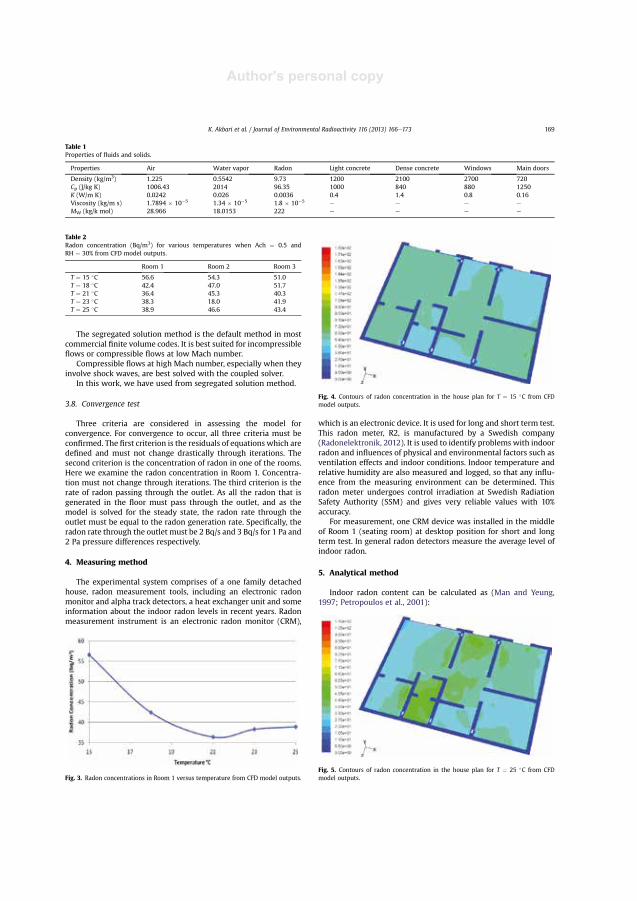
Author's personal copy
The segregated solution method is the default method in mostcommercial finite volume codes. It is best suited for incompressibleflows or compressible flows at low Mach number.
Compressible flows at high Mach number, especially when theyinvolve shock waves, are best solved with the coupled solver.
In this work, we have used from segregated solution method.
3.8. Convergence test
Three criteria are considered in assessing the model forconvergence. For convergence to occur, all three criteria must beconfirmed. The first criterion is the residuals of equations which aredefined and must not change drastically through iterations. Thesecond criterion is the concentration of radon in one of the rooms.Here we examine the radon concentration in Room 1. Concentra-tion must not change through iterations. The third criterion is therate of radon passing through the outlet. As all the radon that isgenerated in the floor must pass through the outlet, and as themodel is solved for the steady state, the radon rate through theoutlet must be equal to the radon generation rate. Specifically, theradon rate through the outlet must be 2 Bq/s and 3 Bq/s for 1 Pa and2 Pa pressure differences respectively.
4. Measuring method
The experimental system comprises of a one family detachedhouse, radon measurement tools, including an electronic radonmonitor and alpha track detectors, a heat exchanger unit and someinformation about the indoor radon levels in recent years. Radonmeasurement instrument is an electronic radon monitor (CRM),
which is an electronic device. It is used for long and short term test.This radon meter, R2, is manufactured by a Swedish company(Radonelektronik, 2012). It is used to identify problems with indoorradon and influences of physical and environmental factors such asventilation effects and indoor conditions. Indoor temperature andrelative humidity are also measured and logged, so that any influ-ence from the measuring environment can be determined. Thisradon meter undergoes control irradiation at Swedish RadiationSafety Authority (SSM) and gives very reliable values with 10%accuracy.
For measurement, one CRM device was installed in the middleof Room 1 (seating room) at desktop position for short and longterm test. In general radon detectors measure the average level ofindoor radon.
5. Analytical method
Indoor radon content can be calculated as (Man and Yeung,1997; Petropoulos et al., 2001):
Table 1Properties of fluids and solids.
Properties Air Water vapor Radon Light concrete Dense concrete Windows Main doors
Density (kg/m3) 1.225 0.5542 9.73 1200 2100 2700 720Cp (J/kg K) 1006.43 2014 96.35 1000 840 880 1250K (W/m K) 0.0242 0.026 0.0036 0.4 1.4 0.8 0.16Viscosity (kg/m s) 1.7894 � 10�5 1.34 � 10�5 1.8 � 10�5 e e e e
MW (kg/k mol) 28.966 18.0153 222 e e e e
Table 2Radon concentration (Bq/m3) for various temperatures when Ach ¼ 0.5 andRH ¼ 30% from CFD model outputs.
Room 1 Room 2 Room 3
T ¼ 15 �C 56.6 54.3 51.0T ¼ 18 �C 42.4 47.0 51.7T ¼ 21 �C 36.4 45.3 40.3T ¼ 23 �C 38.3 18.0 41.9T ¼ 25 �C 38.9 46.6 43.4
Fig. 3. Radon concentrations in Room 1 versus temperature from CFD model outputs.
Fig. 4. Contours of radon concentration in the house plan for T ¼ 15 �C from CFDmodel outputs.
Fig. 5. Contours of radon concentration in the house plan for T ¼ 25 �C from CFDmodel outputs.
K. Akbari et al. / Journal of Environmental Radioactivity 116 (2013) 166e173 169

Author's personal copy
C ¼ EAVðlRn þ lnÞ (9)
Where C (Bq m�3) is indoor radon content at steady state, E(Bq m�2 h�1) is radon exhalation rate, A (m2) is the radon exhala-tion surface (in this study the house floor), V (m3) is the volume ofthe house, lRn (2.1 � 10�6 s�1) is the radon decay constant and lv(h�1) is the air change rate in the house.
For E ¼ 65 Bq m�2 h�1 (Goto et al., 2008) and the given data ofthe case study house, Equation (9) gives indoor radon levels fordifferent ventilation rates (0.0, 0.25, 0.5 and 1.0). These results areshown in Table 5.
6. Results
6.1. Temperature changes
In order to investigate the effect of temperature on radonconcentration, in CFD model, air change rate and relative humidity
are fixed and temperature is varied from 15 �C to 25 �C. Start valuesfor air change rate and relative humidity are 0.5 and 30% respec-tively. Outside temperature is set at 18 �C in the model.
When inside temperature is less than outside temperature, heatis transferred from the outside to the inside. Inside temperaturetherefore increases. This causes a decrease in relative humidity andtherefore radon concentration also decreases. On the other hand,when inside temperature is greater than outside temperature, heatis transferred from inside to the outside, causing the insidetemperature to fall, increasing relative humidity. This increasesradon concentration. Therefore, we would expect radon concen-tration to decrease and then increase as temperature rises from15 �C to 25 �C. Results of CFD model are shown in Table 2.
Radon concentration transport is essentially pressure based(convection mechanism), and higher indoor temperature acts likea weak vacuum cleaner and creates a stack effect phenomenon(Lesieur, 1990). In higher indoor temperatures, diffusion mecha-nism will also increase and boosts the effect of convection mech-anism in radon transport and will decrease indoor radon content.
This behavior is clearly demonstrated in Fig. 3, where radonconcentration from CFD model in Room 1 (seating room) is plottedagainst temperature.
Figs. 4 and 5 show contours of radon concentration aty ¼ 210 cm from the floor at various temperatures from CFD modeloutputs. These figures show the effects of temperature on bothradon concentration and distribution.
Radon measurement with the CRM radon meter providesconfirmation that radon levels show strong correlation with indoortemperature. These results are shown in Fig. 6. This figure is plottedbased on measurement results at air exchange rate Ach ¼ 0.05.
Fig. 6. Radon levels (green) versus temperature (purple) from measurement. (For interpretation of the references to colour in this figure legend, the reader is referred to the webversion of this article.)
Table 3Radon concentration (Bq/m3) for various relative humidities with Ach ¼ 0.25 andT ¼ 18 �C from CFD model outputs
Room 1 Room 2 Room 3
RH ¼ 30% 102.2 94.3 105.3RH ¼ 40% 99.8 92.5 106.5RH ¼ 50% 96.6 93.8 106.7RH ¼ 60% 96.0 93.5 106.6RH ¼ 70% 96.5 97.4 106.8RH ¼ 80% 102.2 93.8 104.6
Fig. 7. Radon concentration in Room 1 versus relative humidity from CFD modeloutputs.
Fig. 8. Contours of radon concentration in the house plan for RH ¼ 30% from CFDmodel outputs.
K. Akbari et al. / Journal of Environmental Radioactivity 116 (2013) 166e173170

Author's personal copy
6.2. Relative humidity changes
In order to investigate the effect of relative humidity on indoorradon concentration, six values of relative humidity are consideredfor a given temperature and air change rate. The relative humidityvalues are 30%, 40%, 50%, 60%, 70%, and 80% and temperature andair change rate are set at 18 �C and 0.25 respectively. The model issolved for these cases and the results of CFD model are shown inTable 3.
Fig. 7 is plotted based on CFD model outputs. This figure showsthe effect of relative humidity on radon concentration in Room 1(seating room). This figure shows that increasing relative humidityincreases water content in the house and decreases the radonconcentration. However, as relative humidity increases further, airdensity increases, and radon in the room cannot rise upwards.Increasing water content in air also leads to lower diffusion coef-ficients and hence shorter diffusion length for radon. The shorterradon length also restricts the height that radon can rise to.
Fig. 7 shows that radon concentration falls as relative humidityincreases from 30% to 60%, and radon concentration increases asrelative humidity increases above 70%.
Figs. 8 and 9 show contours of radon concentration at a positiony ¼ 210 cm from the floor for various relative humidity values.
Figs. 8 and 9 clearly indicate that the relative humidity influ-ences both radon concentration and distribution.
Radon measurement with the CRM radon meter also showstrong correlation with indoor relative humidity. These results areshown in Fig. 10 at Ach ¼ 0.05.
6.3. Air change rate effects
Contours of radon concentration in the house plan at positiony ¼ 210 cm from the floor for various air change rates, from CFDmodel outputs, are shown in Fig. 11. This figure shows qualitativecomparisons of radon concentrations at four different hourly airchange rates ranging from 0.05 to 1.2 Ach. As evident from Fig. 12,
Fig. 10. Radon levels (green) versus relative humidity (blue) frommeasurement. (For interpretation of the references to colour in this figure legend, the reader is referred to the webversion of this article.)
Fig. 11. Contours of radon concentration in the house plan (Room 1) with air change rates 0.05e1.2 Ach from CFD model outputs.
Fig. 9. Contours of radon concentration in the house plan for RH ¼ 70% from CFDmodel outputs.
K. Akbari et al. / Journal of Environmental Radioactivity 116 (2013) 166e173 171

Author's personal copy
different ventilation rates have distinct effects on indoor concen-tration in Room 1 (seating room).
The results of measurements are also shown in Table 4. In orderto show the impact of ventilation rate on radon level, radonconcentrations were measured at three different ventilation rates.Different remedial actions were also considered during measure-ments. Fig. 13 shows the results at three different air change ratesand using of 5 connected sumps, measured with a CRM. The figureshows that measured radon levels were inversely proportional toair exchange rate.
Continuous radon measurements using a CRM also confirmedthat in the indoor temperature range, fluctuating radon levels in thehouse have strong indirect correlation with temperature.
7. Model validation
Model validation was performed using analytical solution fromEquation (9). The numeric differences between numerical simula-tion and analytical calculation results are shown in Table 5.
For quantitative comparisons, the percentage differencebetween the results of estimation by FLUENT and the analyticalcalculations were computed at each ventilation rate. The maximumdifference was found to be below 10%. Measurement data for the
specified house plan were also in good agreement with numericalsimulation results.
8. Discussion
This study shows that indoor conditions, i.e. ventilation rate,temperature and moisture can have a significant effect on indoorradon concentration. These effects are described and demonstratedtheoretically, by numerical simulation and through measurementand are also validated by analytical solution.
Equation (4) shows that increasing indoor temperature resultsin increasing radon diffusion coefficient. Radon transport withinindoor environment is a result of two mechanisms, convectionmechanism and diffusion mechanism. Radon transport byconvection mechanism is due to pressure gradient and airflow. Fora specific air change rate, convection mechanism is constant andtherefore only diffusion mechanism will affect on radon concen-tration and distribution. Increasing diffusion coefficient increasesdiffusion mechanism effect and therefore it boosts the convectionmechanism effect on radon depletion from indoor environmentand reduces radon concentration. Therefore increasing tempera-ture in a specific air change rate and constant relative humidity byincreasing radon diffusion coefficient reduces indoor radoncontent. However, in high diffusion values the situation of radontransport will be complicated and many other parameters shouldalso be considered. The numerical results shown in Fig. 3 confirmthe inverse relationship between temperature and radon level inthe house.
From the relative humidity viewpoint, maximum diffusioncoefficient value occurs within 20%e80% of relative humidity
Table 4Measured indoor radon levels (Bq m�3).
Date and period ATD CRM Ventilation rate Ventilation type Remedial action
2008e2 (2weeks) 3580 � 380 e 0.25 Extract fan No action2010e1 (3months) 1280 � 160 1580 � 158 0.25 HRV Radon sump & sealing2010e04 (3 weeks) 100 � 20 e 0.5 HRV 3 connected sumps2010e3 (12days) e 97 � 10 0.5 HRV 3 connected sumps2010e3 (12days) e 65 � 6 0.5 HRV 3 connected sumps2010e4 (12 days) e 36 � 4 1 HRV 3 connected sumps
Fig. 13. Radon concentrations versus ventilation rate from measurement (5 connected sumps were used).
Fig. 12. Radon concentrations in Room 1 versus air change rate from CFD modeloutputs.
Table 5Indoor radon concentration results in Bq m�3.
Ach Measurement Analytical solution Numerical simulation Difference (%)
0.0 3580 3582 e e
0.25 90 106 107 0.90.5 45 53 55 3.61.2 25 22 20 10.0
K. Akbari et al. / Journal of Environmental Radioactivity 116 (2013) 166e173172

Author's personal copy
(Kotrappa et al., 1976). The affection mechanism of diffusion coef-ficient on radon concentration has been explained in the previousparagraph. Increasing diffusion coefficient leads to decreasing ofradon content. Therefore within mentioned range of relativehumidity, minimum radon concentration will be obtained. Thesame results have been obtained from the numerical simulationwhich is plotted in Fig. 7. In addition, Equation (6) shows thatincreasing indoor temperature increases the saturation vaporpressure, which has a direct effect on total pressure, leading tolower radon levels.
Increasing ventilation rate increases air change rate whichdecreases radon level. In this case, increasing ventilation rate,convection mechanism which is due to pressure gradient will bedominant mechanism in depletion of radon from indoorenvironment.
Results of numerical modeling indicate a strong relationshipbetween ventilation rate, relative humidity, temperature andindoor radon in the thermal comfort range.
9. Conclusions
It is seen that ventilation rate has direct effect on radon level. Inaddition to maintaining a specific ventilation rate and establishingthe desired indoor pressure using a balanced ventilation system, itis necessary to maintain indoor air temperature and relativehumidity within a specific range to minimize radon levels. Theseranges can be determined and depend on radon level, ventilationrate and type, radon mitigation system and climatic conditions.
In this case study, it is shown that setting temperature between20 and 22 �C and relative humidity between 50 and 60% in a specificair change rate can affect on indoor radon levels.
The 3D models developed with FLUENT simulated radon entrythrough the floor into a one family house. The overall resultsindicate that indoor radon concentrations are dependent onventilation rate, indoor temperature and moisture levels. Theverification of the model and its performance support the idea thatradon entry to the house and effects of ventilation rate, tempera-ture and moisture can be defined well physically and numerically.The performance and sensitivity of the model was confirmed byvarying input parameters and boundary conditions. The resultsindicate that the considered conditions and assumptions providedacceptable modeling of this environment. This model may there-fore be useful and applicable for other similar problems undera similar range of conditions.
This model may be improved by considering additionalparameters that occur in real situations in residential buildings,such as wall temperature, internal heating sources and externalsituations and temperature differences between the inside andoutside. The problem can be modeled with the integration of all orsome combinations of these to reflect real weather conditions. Inaddition, more detailed treatment of turbulence and wall effectsand a finer grid near the sourcemay also improve CFD performance.
In conclusion, CFD is a powerful tool for exploring the factorsthat influence radon distribution in a residential building. However,the accuracy of indoor radon and indoor conditions simulationresults can only be confirmed for conditions that have beenvalidated.
References
Andersen, C.E., 2001. Numerical modeling of radon-222 entry into houses: anoutline of techniques and results. J. Sci. Total Environ. 272, 33e42.
Clever, H.L., 1979. Solubility Data Series. In: Krypton, Xenon and Radon Gas Solu-bility, vol. 2. Pergamon Press, Oxford.
FLUENT Incorporation, 2005. FLUENT User’s Guide Version 6.3. FLUENT Inc.,Lebanon, NH, USA.
Goto, M., Moriizumi, J., Yamazawa, H., Iida, T., Zhuo, W., 2008. Estimation of globalradon exhalation rate distribution. In: Proc. of 8th Int. Symp. Natural RadiationEnvironment-AIP Conference, Buzios, Brazil, vol. 1034, pp, 169e172.
Kotrappa, P., Bhanti, D.P., Raghunath, B., 1976. Diffusion coefficients for unattacheddecay products of thoron-dependence on ventilation and relative humidity.J. Health Phys. 31, 378e380.
Lesieur, M., 1990. Turbulence in Fluids. Kluwer Academic Publisher, Dordrecht, TheNetherlands.
Man, C.K., Yeung, H.S., 1997. The effects of cracks and holes on the exhalation ofradon from concrete. J. Build. Environ. 32 (4), 351e354.
Petropoulos, N.P., Anagnostakis, M.J., Simopoulos, S.E., 2001. Building materialsradon exhalation rate: ERRICCA intercomparison exercise results. J. Sci. TotalEnviron. 272 (1e3), 109e118.
Radonelektronik, 2012. Available at: www.radonelektronik.se (accessed 10.05.12.).Sonntag, D., 1990. Important new values of physical constants of 1986, vapour
pressure formulations based on the ITS-90, and Psychrometer Formulae. J. Z.Meteorol. 40 (5), 340e344.
Stranden, E., Kolstad, A.K., Lind, B., 1984. The influence of moisture and temperatureon radon exhalation. J. Radiat. Protect. Dosim. 7 (1e4), 55e58.
Sun, H., Stowell, R.R., Keener, H.M., Michel, F.C., 2002. Two-dimensional computa-tional fluid dynamics (CFD) modeling of air velocity and ammonia distributionin a high-rise (TM) Hog building. Trans. ASAE 45 (5), 1559e1568.
Surbeck, H., 1996. A radon in water monitor based on fast gas transfer membranes.In: Proc. Int. Conf. on Technologically Enhanced Natural Radioactivity, Poland,pp. 16e19.
Van der Pal, M., Van der Spoel, W.H., 2001. A simple method for measuring radonadsorption in porous materials. In: Proc. Workshop Radon in the Living Envi-ronment, Liege, Belgium.
Wang, F., Ward, I.C., 2000. The development of a radon entry model for a house witha cellar. J. Build. Environ. 35, 615e631.
K. Akbari et al. / Journal of Environmental Radioactivity 116 (2013) 166e173 173

