skin and proximity effect analysis of traction motor ricardo - diva
TRANSCRIPT

1
Skin and proximity effect analysis of traction motor
Ricardo Huaytia
Supervisor:
Torbjörn Trostén
Examinator:
Chandur Sadarangani
Master Thesis
Royal Institute of Technology
School of Electrical Engineering
Electrical Energy Conversion
Stockholm 2012
XR-EE-E2C 2012:005

2
Sammanfattning
Traktionsmotorer är termiskt pressade för att få ut högt moment per volymenhet samtidigt som en relativt hög frekvens används. På grund av den höga frekvensen är fenomenet strömförträgning samt närhetsinverkan ett område som borde utforskas. Kopplingen mellan dessa parasitiska egenskaper och termisk påverkan mot isoleringen är viktig att förstå. I examensarbetet har en FEM-modell i Flux 2D lämpat för strömförträgnings analys tagits fram. Termiska nätverk har tagits fram för att hitta lokala termiska stresspunkter. I denna studie har sinus matning i två driftpunkter studerats men även triangulär sinus PWM matning för nominell driftpunkt studeras.
Nyckelord: Partnivå FE modell, Induktionsmotor traktion, strömförträgnings värmeförluster, FEM, termiskt nätverk av statorspår i partnivå
Summary
Traction motors are thermally pressed to obtain a high torque per unit volume at the same time as a relatively high frequency is used. Because of the high frequency the phenomenon skin effect and proximity effects appear, this is explored in the thesis. To find a link between the parasitic and thermal effects on the insulation is important. In this thesis, a finite element model of the Flux 2D suitable for skin effect analysis is developed; also a thermal network has been developed to find thermal hotspots in the stator slot. In this thesis, sinusoidal supplies for two operating points are studied and triangular sinusoidal PWM supply is as well studied for the nominal operating point.
Keywords: Strand-level FE model, induction traction motor, skin effect thermal losses, FEM , strand level stator analytical thermal network

3
Acknowledgments
Since the start of this thesis on 24th of October 2012 I had the best period of my studies doing my thesis at ABB machines realizing this project. During this period I noticed the importance of the atmosphere and environment at the office, in the end, enjoying the colleagues can be decisive. I was lucky to get the opportunity to do my master thesis at the traction group and my beautiful experiences from the department will not be forgotten. Huge gratitude is given to my examinator professor Chandur Sadarangani, technical manager Stefan Palmgren and R&D manager Ola Aglén who made this possible.
At the moment of writing this report I specially want to thank Fabio Guidi, Cedric Monnay, David Lindberg, Björn Larsson, Chandana Ragipani and Xi Yang for all the fun moments and laughs that were shared inside and outside the office. My supervisor Torbjörn Trostén has been the ideal supervisor for this thesis both for his deep knowledge but also for his great personality.
My family and friends that have made my time at my hometown Västerås to the best place ever, Roger Huaytia my beloved brother that supported and encourage me during my entire studies and specially during my thesis, special thanks to Milena for all understanding and support.
Last but not least my dear father and my dear mother that always believed in me and supported me with everything.
To all of you, I want to say thanks.
Q-building floor 2, KTH, Stockholm 2012-03-26

4
Contents 1 Introduction
1.1 Background 1.2 Objectives and scope 1.3 Outline of thesis
2 Literature studies 2.1 Traction induction motor 2.2 Equivalent circuit diagram 2.3 Skin effect
2.3.1 Solid stator conductor 2.3.2 Stranded conductor 2.3.3 Skin effect theory 2.3.4 Analytical formulas 2.3.5 Proximity effect 2.3.6 Transpose of winding 2.3.7 Fractional winding
2.4 Thermal modeling 2.4.1 Basic thermal analysis theory 2.4.2 FEM thermal model 2.4.3 Analytical LP thermal model 2.4.4 Steady state 2.4.5 Dynamic state
2.5 FEM analysis 2.5.1 FEM theory 2.5.2 Geometry 2.5.3 Electrical circuit coupling
2.5.3.1 Stator 2.5.3.2 Rotor
2.5.4 Mesh 3 Strand-level FE model of the stator slot
3.1 The geometry before and after 3.2 Stator winding 3.3 Working method 3.4 Mesh 3.5 Validation model without strands vs. strand model
3.5.1 55 Hz at steady state 3.5.2 110 Hz at steady state
4 Thermal network for stator slot 4.1 Solid conductor
4.1.1 Section one 4.1.2 Section two 4.1.3 Section three
4.2 Double solid conductor

5
4.2.1 Section three 4.3 Stranded conductor
4.3.1 Section four A 4.3.2 Section four B
4.4 The LP-model
5 Result analysis 5.1 Current density distribution at frequencies 55 Hz and 110 Hz
5.1.1 Sinus source - 55 Hz 5.1.2 Sinus source – 110 Hz
5.2 PWM - 55 Hz fundamental 5.3 Losses in strands
5.3.1 Sinus 55 Hz 5.3.2 Sinus 110 Hz 5.3.3 PWM 55 Hz fundamental
5.4 Skin effect temperature rise for PWM 55 Hz, sinus 55 Hz and sinus 110 Hz 6 Conclusion and future work
Bibliography Appendix

6
List of symbols
FE = Finite-element
ECD = Equivalent Circuit Diagram
DOL= Direct on line
VSI=Voltage source inverter
FEM= Finite-element Method
J= Current density
B= Flux density
DCR = DC resistance
ACR = AC resistance
RMS= Root Mean Square
SÂ =Current loading in stator, magnitude
RÂ = Current loading in stator, magnitude
iI = Total current in slot i
s = Slip
mn = Mechanical speed in rpm
sn = Synchronous speed in rpm
1R = Stator resistance
e = Induced voltage
skinδ =Skin depth
Pτ = Full pitch
y = Coil pitch
p = Number of poles
q = Number of slots per pole and phase
sQ = Stator slots

7
1 Introduction In electrical design the ideal motor is the motor with superconductors, no leakage flux in slots, perfect sinus source, perfect linear iron without saturation and approximately 100% efficiency. This is of course not possible and one factor is the thermal limitation, similar as in power electronics and power system. The demand on super-efficient machine is big due to the life operation cost of an industrial electrical machine. As electrical machine producer the challenge is to deliver due to additional losses in stator windings.
1.1 Background
Differences between the electrical asynchronous traction motor and the traditional industrial asynchronous motor are [2]
- limited space in the bogie - High torque/shaft length - High running temperature
The delivered torque from a motor is expressed by following equation
(1.1)
Where D is air gap diameter [m], L is the active length [m], 𝑅 is the current loading in rotor [A/m],
𝐵𝛿 the air gap density and β is angle between rotor current loading and air gap flux density. As we can see the torque is strictly proportional to motor physical dimensions and β.
• β is controlled with power electronics, if the motor is direct to line it will be in range 5° - 10° degrees [1], we want β to be as small as possible to maximize the output torque
• 𝐷2 is restricted by limited space in bogie
• L is restricted by limited space in bogie
• 𝑅 is restricted by thermal limits on insulation in stator slot
• 𝐵𝛿 is restricted by iron saturation
2
cos4 R
DT L A Bδπ β=

8
The challenge is to maximize 𝑅 . The phasor diagram for this equation can be calculated.
Figure 1-1. Phasor diagram for an induction machine [1]
As it can be seen in equation (1.2) one way for a given motor to maximize the current loading of the rotor is to either maximize the power factor or by maximizing the current loading of the stator.
cos( )r s  ϕ=
(1.2)
1
nii
Sconductor span
IÂ
l== ∑
(1.3)
Where 𝐼𝑖 is the current in conductor i and 𝑙𝑐𝑜𝑛𝑑𝑢𝑐𝑡𝑜𝑟 𝑠𝑝𝑎𝑛 the periphery length of conductor segment.
To visualize𝑆, the example in figure 1-2 is presented.
Figure 1-2.Illustration of 𝑆
𝑆 =4 𝐴 + 4 𝐴 + 4 𝐴
0.4 𝑚= 30
𝐴𝑚

9
The challenge is to maximize the current through the stator slot combined with respect to the limits of the power electronics in VSI. To accomplish the first part, better thermal understanding of the stator slot is needed.
1.2 Objectives and scope
There are two objectives in this work.
Develop a detailed FEM model in Flux 2D that includes a strand level stator slot geometry. The model will then be used for skin effect analysis. In the thesis some results will be presented but the aim is to develop a suitable FEM model for skin effect analysis.
A good and simplified model is to assume that whole stator slot is filled with a “stranded coil”. This is shown in figure 2.
Figure 1-3. Simple stator slot model with ELECTRIFLUX “stranded coil conductor”-component
Figure 1-4. A-phase part of simple stator slot model with ELECTRIFLUX “stranded coil conductor”-component
Where SS1AP1p1 is the coil component that model half of the active part of a coil group in phase A, SS1AM1p1 the other half, S1AR1 the resistance of the endwinding and S1AL1 the inductance of the end winding.
A FEM simulation with more detailed stator conductor geometry is needed. The detailed strand level stator slot conductor is presented in figure 4.

10
Figure 1-5. Strand level stator slot that will be used in this thesis
Figure 1-6. Half of A-phase in strand level stator slot using solid conductor for each strand
Second part of the work will be developing a thermal network (also called lumped model) for the strand level stator slot in figure 4. This network will be used for fast calculation of the temperature rise when taking skin effect losses into account in the heat sources.
1.3 Outline of the thesis
Chapter 1 – Introduction of thesis
Chapter 2 - What has been done and by who. Literature studies
Chapter 3 – The stranded FE- model work will be presented and explained
Chapter 4 – Explanation of the thermal network
Chapter 5 – The results will be analyzed and presented
Chapter 6 – What is the conclusion of this thesis and how can ABB Traction use it. What more can be done

11
2 Literature studies
2.1 Traction induction motor
The studied traction motor is used in the electrical railway traction and is the last component in the electrical drive system.
Figure 2-1. Electrical drive system for railway traction
The standstill asynchronous traction motor can be represented with an equivalent three phase circuit. When the motor is at standstill it behaves identical to a transformer with winding turn ration 1:s and s=1, where s is the slip ratio of the mechanical rotor velocity relative the air gap flux velocity in percentage.
𝑠 = 𝑛𝑠−𝑛𝑚𝑛𝑠
(2.1)
2.2 Equivalent circuit diagram
The easiest way for making fast calculations of an induction motor is by using the ECD. There are different types of circuit diagrams but the T-model is preferred in this thesis. Another representation is the gamma – model and is most suitable in control applications. The voltage drop on the rotor side is pure inductive in some models this inductance is included in the rotor inductance.
T-ECD

12
Figure 2-2. Equivalent circuit diagram T-model
The analytical method for setting of all components are in literature and can be found in [1].
GAMMA-ECD
Figure 2-3. Equivalent circuit diagram GAMMA-model
The analytical method for setting the leakage flux is in literature [3].
Both ECD are very good models that can be adapted for the wanted information. The ECD is commonly used with the assumption that the stator has a sinusoidal distributed winding. This leads to and perfect output torque without ripples. If non linearities and slot harmonics are meant to be included, FEM simulations are really good. If we want to model the skin effect losses in the ECD they will be included as circulating currents in R1, Rr’ and Rm. In this thesis the active losses will be investigated. Analytical formulas for the skin effect is well known but not for the proximity effect. The motor losses mostly includes following components.
𝑃𝑐𝑢 - Copper losses in the stator and rotor (rotor can be aluminium)
𝑃𝑓𝑒 – Total iron losses
𝑃𝑠𝑡 – Fundamental stray load losses
𝑃ℎ - Harmonic stray losses
Copper and iron losses are shown in the ECD. Stray losses are the losses, that by definition refer to the additional losses that occur in a machine over the normal losses that are considered in usual performance calculation for motor efficiency [1]. These additional losses in ECD are partly built up by skin effect and proximity effect losses. The skin effect can be taken into account but proximity losses are not as easy to predict.

13
2.3 Skin effect
2.3.1 Solid conductor
First case is the solid copper conductor in stator slot fed with DC voltage. If a DC current flows through the copper the flux density produced by the conductor will increase proportional with the height of the conductor. To show this J(h) and B(h) will be presented [3], where J(h) is the current density as function of height h[m] and B(h) is the flux density as function of height h[m].
Figure 2-4 a). Height increasing Ampere loops Figure 2-4 b).Flux density vs height Figure 2-4 c) Flux density vs height.
Second case is the solid copper conductor in stator slot fed with AC voltage. Because of the skin effect the current density will be no uniformed. Closer to the air gap the current density increases. A graph is shown to illustrate the shape [1].
Figure 2-5 a). Flux density vs. height, AC source Figure 2-5 b). Current density vs. height, AC source
If we increase the frequency the skin effect will be even more aggressive [1].
Figure 2-6 a). Flux density vs. height, high freq. AC source Figure 2-6 b). Current density vs. height, high freq. AC source

14
2.3.2 Stranded conductor
An established technique to reduce the skin effect is by increasing the number of strands nh in a slot. Let’s discuss the following geometry.
Figure 2-7. Stranded conductor with three strands
If the strands are series coupled all strands will have the same current. First let’s assume DC, the current density will result in following.
Figure 2-8 a). Flux density vs. height, DC source Figure 2-8 b). Current density vs. height, DC source
Second case is when applying AC voltage with medium high frequency. This is the same as in [1] but taking strands into account, the same behavior of a solid body will repeat itself. This result have been presented in [14] figure 4-4.
Figure 2-9 a). Flux density vs. height, AC source Figure 2-9 b). Current density vs. height, AC source

15
The current density of the prototype with low frequency, higher frequency and PWM (very high frequency) are presented in chapter 5.1 and chapter 5.2. The graphs can be studied using Maxwell’s fourth equation also known by the name Amperes law when assuming that the electrical density is not time dependent. To see the derivation of this volume integral the reader is assigned to [].
DH Jt
∂∇× = +
∂
2.3.3 Skin effect theory
In high school we learned the right hand rule for prediction of direction of field B produced by a single conductor. This is an easy and fast tool for prediction of the path of magnetic flux. Though, it is assumed that the diameter of the conductor is infinite small and no flux density will perpendicular cross the conductor itself.
If we neglect this assumption a new phenomenon appears. Because of the new bigger diameter in the conductor the flux density will not only be in the surrounding space. Flux density lines will now appear in the conductor cross sectional space and cross the conductor. A fundamental law is following.
BEt
∂∇× = −
∂ (2.2)
Where E is the electrical vector field and B is the electrical flux density.
In faraday’s law of induction a minus sign is also written and this is because of Lenz law. The negative sign shows that the induced voltage and the change in flux density have opposite signs in respect to time.
This is Maxwell’s third equation also known by the name faradays law. To see this the volume integral can be made on both sides and by using Stokes law. The magnetic flux that is produced from the conductor will induce a voltage in the same flux producing conductor and this is repeated. This will result with non-distributed current in the conductor. Notice that if B is not varying in time and space (DC current) this phenomenon will not appear. It is possible to separate the flux into two types of flux, internal and external flux. The internal flux is the flux that will contribute to the uniform current distribution and the external flux is the flux that will couple the stator with the rotor. The non uniform current distribution will result in a smaller cross path area of the conductor and will thereby result in a higher resistivity; this is analytically found as a skin effect impedance coefficient in the ECD for the stator, and rotor. It is very easy to find the analytical formulas for calculation of the skin effect impedance factor, these are presented in 2.3.4.
2.3.3.1 Skin depth
An important parameter in this topic is the “skin depth” and is defined in 2.3.4 as parameter skinδ in
equation (2.4). This is the ratio between the height of the conductor and the pierce depth of current
density. If skinδ is equal to infinity is means that the position of pierce is significant higher than the
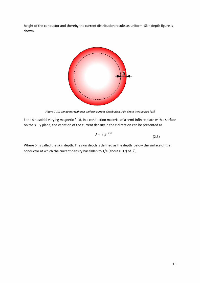
16
height of the conductor and thereby the current distribution results as uniform. Skin depth figure is shown.
Figure 2-10. Conductor with non-uniform current distribution, skin depth is visualized [15]
For a sinusoidal varying magnetic field, in a conduction material of a semi-infinite plate with a surface on the x – y plane, the variation of the current density in the z-direction can be presented as
/d
sJ J e δ−= (2.3)
Whereδ is called the skin depth. The skin depth is defined as the depth below the surface of the
conductor at which the current density has fallen to 1/e (about 0.37) of sJ .

17
2.3.4 Analytical formulas
Skin effect is a well-known phenomenon and during last decade these formulas have been well established. In this chapter the analytical formulas for skin effect and proximity effect for one slot will be presented. The proximity effect concept is related to the skin effect phenomena, this proximity concept will be discussed in subchapter 2.2.5.
0 1
cuskin f
ρδµ π
= (2.4)
skin s
h bebδ
= (2.5)
sinh 2 sin 2( )cosh 2 cos 2
e ef e ee e+
=− (2.6)
sinh sin( ) 2cosh cos
e eg e ee e−
=+ (2.7)
( ) ( )1 ( 1)strandK f e p p g e= + − (2.8)
( ) 1 ( )
3h
slotnK f e g e−
= + (2.9)
Where h, b and bs can be found in figure.
skinδ - Skin depth [ m ]
cuρ - Resistivity of copper [ mΩ⋅ ]
f - Frequency of current flowing through [Hz]
p - Number on conductor with 1 in slot bottom close to the yoke [no dimension]
hn - Number of conductors in slot [no dimension]
These formulas are from [1] and [13].
slotK is the resistive skin effect factor and all losses that this factor produced are the skin effect
losses. The effective cross area of the conductor will be smaller due to the concentration of current density. In this set of formulas there is no flux density dependent factor due to the global flux that crosses the slot. These losses are identified as global proximity losses and are explained in 2.2.5.

18
2.3.5 Proximity effect
In subchapter 2.3.3 the concept of skin effect was explained with faradays law and external-internal flux. Subchapter 2.2.4 introduced more than one conductor per slot and thereby proximity effect. If many conductors are close to each other the flux from conductor one will obviously cross the nearby conductors and some circulating current will appear which leads to more conductor losses.
Proximity losses can be divided into two different losses, internal and global proximity losses. Eq. (2.10) includes both phenomenas and Eq. (2.6)-(2.7) only includes the internal proximity losses. In most electrical machines the number of slots in stator is bigger than one, why this global proximity effect have to be taken into regard. In literature [19] the proximity losses are investigated but no analytical formula is suggested. In [19] a PMBL machine is studied and the proximity effect losses are studied. An analytical formula for PWM source is suggested
4 2 2
128n
ec
d BP π ωρ
= (2.10)
Where d and cρ are the diameter and resistivity of conductor, respectively, nB and ω are the
peak value and angular velocity of flux density harmonic respectively. As shown in the formula the proximity losses depends on three things, copper area, electrical frequency and flux density in slot.
The formula should according to the authors be applicable to other machines than in the study.
Figure 2-11. Illustration of the flux densitys influence on proximity losses in Eq(2.10) [19]

19
2.3.6 Transpose of winding
By transposing the winding it is possible to reduce the proximity losses. There is winding methods that are suited for this types of consideration, one is the famous Roebel winding. This is crucial when having parallel strand in the slot. For further reading read [20].
2.3.7 Fractional winding
In double layer electrical machines fractional pitch is often implemented. In this scenario all conductors in one slot will not always have the same electrical phase angle. The resistive skin effect factor of these slots having this combination of coils are reduced [5].
Phase angel between the currents 120 degrees
Correction factor 0,40
Table 1. Correction factor for the additional losses
2.4 Thermal modeling
2.4.1 Basic thermal analysis theory
An electrical engineer works with electrical circuits. LP-network method is known for a long time and the method is established in softwares as MOTORCAD and in analytical research studies. To model other engineering problems using electrical circuits is beneficial. To completely understand the electrical machine the thermal, mechanic and electrical knowledge is important. There is an analogy between these three topics and many of problems in the above engineering topics can be modeled and solved with a lumped electrical circuit.
To show this analogy see table 1.
Thermal network Electrical network Temperature difference (K) Voltage (V) Heat transfer (losses) (W) Current (A) Heat resistance (conductance) (K/W) Electric resistance (conductance) (V/A) Heat capacitance (Ws/K) Electric capacitance (As/V)
Table 2 .Table for analogy between thermal and electrical networks [1]
Table and following laws makes the thermal lumped circuit model complete:
- Thermal resistances rather than electrical resistances - Power sources rather than current sources - Thermal capacitances rather than electrical capacitors - Nodal temperatures rather than voltages - Power flow through resistances rather than current.
There are different ways to transfer heat.

20
Conduction
Thermal heat flows through a material. The substance can be in any state, solid, liquid or gas. This happens in the iron. The thermal resistance are in conduction modeled as (2.11).
thLRAλ
= (2.11)
Where L is the length of geometry [m], k thermal conductivity of material [] and A path area of heat
flow (A is perpendicular to the direction of the heat flow)[(m ⋅ K)/W]. The dimension of thR is [K/W].
Convection
Heat is transferred by the movement of a substance. Air is a typical substance and is used in air gap and air ducts. The fan that is mounted on shaft uses convection to cool the machine. Thermal resistances are modeled with (2.12)
thLR
hA=
Where h is the heat transfer coefficient and have dimension [(m 2 ⋅ C)/W]. In convection heat transfer there is free convection and forced convection. Free convection is the natural convection, which is a result of the boundary force caused by the variation of the medium’s density [15]. Forced convection is made by an external fan or pump [15].
Thermal radiation
Thermal radiation is electromagnetic radiation generated by thermal motion of charged particles in matter. As long as the matter has a temperature bigger than zero it emits thermal heat due to radiation. The sun is transmitting heat with thermal radiation, also the earth but with much lower intensity [18]. Net radiation that leaves a surface depends on area, material characteristics, temperature, and surroundings [17]. The net radiation from a body to the surroundings can be calculated by [17]
( )4 4
wq T Tσε ∞= − (2.11)
Where wT and T∞ are the absolute temperatures of the body and the surroundings, respectively, is
Stefan-Boltzmann’s constant and e is the emissivity if the body. In such a case, the thermal resistance to the surroundings is [17]
4 4( )
wth
w
T TRA T Tσε
∞
∞
−=
− (2.12)

21
2.4.2 FEM thermal model
The FEM thermal model is done in same environment as the electromagnetic simulations. The biggest differences are that there is no need to set the electric circuit. Geometry and physics are still needed with some thermal boundaries and heat sources assigned. FEM analysis for electromagnetic simulations will be introduced in subchapter 2.5.1.
2.4.3 Analytic LP thermal model
An analytic thermal model is a circuit that you build up analytically from the geomtry of the machine or component that is modelled. All volumes are represented as thermal resistances in two directions. For the cylindrical shaped electrical machine, angular and radial directions are applied.
2.4.4 Steady state
In steady state modeling there is no thermal capacitances. The circuit can be solved as a dc circuit and as we know from circuit theory all capacitance behaves as infinite impedance. The currents and voltages will not vary with respect to the time.
2.4.5 Dynamic state
In dynamic state analysis there is need to use thermal capacitances. Thermal capacitances for transient analyses are C=Weight*Specific Heat Capacity of material.
The thesis will not take dynamic state analysis into regard, this because in thermal aspect the hotspot is of major interest.
2.5 FEM analysis
2.5.1 FEM theory
When designing electrical machines the designer first make rough calculations of the design with analytical equations and the ECD. A powerful tool to take most of the nonlinearities and non-ideal phenomena into account is the FEM program CEDRATS Flux 2D. The use of a two dimensional FEM version will require further approximations of the 3D properties that the real machine have [1].
2.5.2 Geometry
The designer have all preliminary geometry data. This data is used to build up the geometry of the active cross section. When working with FEM, building up the geometry is the first step. During the first step symmetry is an advantage and can be used. By implementing symmetry the computation time will be considerably shorted.
2.5.3 Electrical circuit coupling
Flux 2D have been used and in this software we model the active length in geometry. The subsoftware that is included in Flux 2D is called ELECTRIFLUX. In ELECTRIFLUX an electrical circuit is designed and represents the environment of the electrical machine.

22
2.5.3.1 Stator
As seen in figure only the active part is modeled in geometry. The machine is not only dependent on active geometry. Somewhere a coupling between the rest of electrical parameters and this is done in ELECTRIFLUX where we can build up and electrical circuit for the project. In the FEM box all strands are modeled as solid conductors.
Figure 2-12. FEM model coupled with the external equivalent circuit
2.5.3.2 Rotor
The same thing is done with the rotor. Short circuited rotor is sectioned to three parts.
Short circuit ring, excluding the rotor bar ends. The component Zring in the rotor equivalent circuit is the impedance between two rotor bar ends.
Active part of rotor bars. The rotor bars are the torque producing components in the rotor. The current loading in the rotor is an important factor for the produced torque, se equation [].
Rotor bar ends. A casted rotor has iron surrounding the active part of the rotor. The rotor bars have rotor bar ends and these parts are outside the iron and active length.
Computation formulas are found in [1].
Figure 2-13. Short circuit ring used in FEM model

23
In the rotor geometry the active parts of the rotor bar are modeled. In figure 2-13 the modeled components are called FEM. 2Zbe is the impedance of two rotor bar ends.For deeper understanding the reader is assigned litterature [1].
2.5.4 Mesh
Until now no “finite elements” are used. The meshes will introduction these elements to the model. Every region is subdivided in finite elements and Maxwell’s equations will be solved for these entire region.
Figure 2-14. Finite element defined from meshing the domain
By making the mesh the designers is given the computer the shape and numbers of elements in geometry. For skin effect the importance is in stator slot so fine mesh in this region will be used. The shaft in this model will not have such as fine mesh. The numbers of elements is directly proportional to the solving time and FEM simulation is already well known for its long solving time. Because of this reason the mesh have to be designed in a smart way.

24
3 Strand-level FE model of the stator slot
3.1 The geometry with and without strands
The model that will be developed has coil components in the electrical circuit. As shown in figure 3-1 the new model will result in a simplified stator slot winding geometry. There is no possibility to see the strands in the geometry. The numbers of strand per coil is set in the electrical circuit as an input value in the coil component.
Figure 3-1. Complete geometry with coil component and no strands
During the thesis a new stranded model have been developed. As shown in figure the strands also appear in the geometry. It is also possible to see how many components in the electrical circuit every coil component models.
Figure 3-2. Complete geometry with solid conductor components and strand

25
To see the difference more clearly slot 42 and 43 is shown in both cases.
Figure 3-3. Slot 42 with same phases in both layers and slot 43 with mixed phases
Figure 3-4. Slot 42 and slot 43 with stranded conductors
Insulation has also been included in the stranded geometry. This region has been assigned as “air or vacuum region”. Assumption made here is that the spacer is of same material as conductor insulation. The reason is simplification in geometry.

26
3.2 Stator winding
To develop the strand level model it is important to understand how the stator winding is arranged. The complete winding of the prototype is presented in appendix A.
As we see in appendix A
- Each phase have four coils in series due to numbers of poles, p =4.
- The number of slots per pole and phase q = 4.
- The total number of stator slots sQ =48.
- The total number of slots per phase is p q⋅ = 16.
- Full pitch, pτ =48/4= 12
- Coil span, y is 10 slots (from slot 6 to 44).
- Pitch factor, / py τ =10/12
Because of symmetry I will study two coils of the Q1/q=12, starting at slot six (from bottom to top layer).
Figure 3-5. One coil with electric current from bottom layer to top layer

27
The second coil is from top to bottom.
In appendix B the winding of strand is presented. In slot 6 there is eight different positions B1, B2, B3, B4, T1, T2, T3 and T4.
The strands in one coil change positions on their way from slot 6 to slot 44.
Slot 6 Slot 44
Figure 3-6 a). Strand position in stator slot in a half turn Figure 3-6 a). Strand position in stator slot in the second half turn
The change of position will be implemented in ELECTRIFLUX when designing the coupled electrical circuit. This will be done in all 24 slots.
In the ELECTRIFLUX there is two different ways to model a coil.
First it is possible to model the coil with a stranded coil conductor where you set the number of strands, notice that the component is no copper component.
Figure 3-7. Electrical circuit where the A-phase winding is modeled with two coil components
Here SS1AP1p1 is half of the coil where the current direction is positive. In SS1AM1p1 the polarity of the component is opposite of SS1AP1p1 and this component is the other half part of the coil where the current is negative.
It is also possible to model the coil with sn q⋅ =8 4⋅ =32 solid conductor components per coil
component.
A2
A1
A7
A5
A6
A7
A8
A3
A4
A3
A4
A5
A6
A2
A8 A1

28
Where
- sn is the number of strands
- q is the number of slots per pole and phase
If the conductors are modeled with coil component the conductor regions in the stator slots will not show the skin effect or current density in the graphical post processor. To see the skin effect the second method needs to be implemented.
Figure 3-8. Electrical circuit where the A-phase winding is modeled with 64 solid conductor components
The number of solid conductors for the complete motor is sn q p⋅ ⋅ = 8 ⋅ 4 ⋅ 4 = 128 per phase. This is
the second and correct way to model the slot for skin effect studies. Skin effect phenomena are showed in solid conductors as the rotor bars.
Figure 3-9. Current density is computed in stator and rotor slot in new model
Color Shade Results
29
3.3 Working method
Simulations with stranded coil component will be presented and the losses in stator slot will be analyzed. Simulations results from solid conductor components will be compared with simulation one. Also here the stator slot will be analyzed and differences will be discussed.
3.4 Mesh
In FEM analysis the mesh construction is without doubt the most time consuming step in defining a problem.
The basic ground rules are summarized as following:
• The finite elements should be well proportioned
• Ideal finite element is a equilateral triangle or square
• Mesh should not be unnecessarily fine
There are two types of mesh that is applied in this project. Automatic mesh and mixed mesh. Mixed mesh is more adaptable for the regions physics. In this project it is suitable for the meshing of strands and the insulation between them.
ABB in house software generates FEM geometry with its mesh. In this thesis optimization of the mesh in the whole machine is not the aim. Existing mesh is used as much as possible with some modifications on the stator slot, tooth and yoke. For skin effect simulations Cedrat recommends mapped mesh in the solid conductors.

30
Model without strands:
Figure 3-10.Mesh with coil components before implementation of strands
Strand model:
Figure 3-11.Strands are implemented and new mesh have been generated

31
Mesh data model with strands:
Number of nodes 77219 Number of line elements 11425 Number of surface elements 33404 Number of elements not evaluated 0 % Number of excellent quality elements 77.25 % Number of good quality elements 15.62 % Number of average quality elements 4.16 % Number of poor quality elements 2.96 % Number of abnormal elements 0%
Table 3.Mesh information for the geometry in the stranded model
3.5 Validation model without strand vs. strand model at 55 Hz and 110 Hz in steady state current
The models with coil components and no stranded conductors in geometry are used for verification. Both of the models should have same stator currents with some minor differences. The voltages applied to both models are not equal; this is built on long experience and is.
3.5.1 Frequency 55 Hz at steady state
Figure 3-12. Stator current vs. time in phase A at steady state with RMS value 185.7 A, no strand model at 55 Hz-sinusoidal
By studying figure 3-12 following statements can be made:
• Root mean square value of stator current is 185.7 A
• Stator current is sinusoidal
• Frequency is 55 Hz

32
Figure 3-13. Stator current vs. time in phase A at steady state with RMS value 185.2 A, stranded model at 55 Hz-sinusoidal
By studying figure 3-13 following statements can be made:
1. Root mean square value of stator current is 185.2 A 2. Stator current is sinusoidal 3. Frequency is 55 Hz
Differences in the both models are less than 1 %.
3.5.2 Frequency 110 Hz at steady state
In this simulation the geometry is identical to the one used in 55 Hz simulations. To change frequency the electrical circuit is changed and the voltage sources have 110 Hz as frequency.
Figure 3-14. Stator current in phase A at steady state with RMS value 171.4 A at 110 Hz-sinusoidal

33
By studying figure 3-14 following statements can be made:
1. Root mean square value of stator current is 171.4 A 2. Stator current is sinusoidal 3. Frequency is 110 Hz
Figure 3-15. Stator current in phase A at steady state with RMS value 170.9 A at 110 Hz-sinusoidal By studying figure 3-15 following statements can be made:
1. Root mean square value of stator current is 170.9 A 2. Stator current is sinusoidal 3. Frequency is 110 Hz
Differences in the both models are less than 1 %.
3.6 Summary
A new stranded FEM model has been developed. The electrical circuit has a solid conductor per each geometric strand, with these new components Flux 2D is able to do all calculations needed for skin effect analysis. All strands are transposed and full knowledge of the winding is needed in this work. Meshing is important and the number of elements can be reduced by a skilled and experienced FEM user. All finite elements with poor quality are in the rotor and will not affect the calculations in the stator.
Verifications have been done and the model is trustworthy.

34
4 Thermal networks for stator slot
The aim is to develop a thermal network for calculation temperature rice in different nodes. First case is to assume solid copper. Second case will be for ns conductors. Because of symmetry only the heat transfer to one tooth will be investigated.
4.1 Solid conductor
The first way to model a stator slot is assuming that the copper in a stator slot is solid, this is very common and used in many thermal models for electrical motors. In this case we section the stator slot to three radial sections.
Figure 4-1 a). Solid conductor FEM-model divided in three sections Figure 4-1 b). Thermal network for half of figure4-1
Because the cylindrical shape of the stator and specially the stator tooth there is a need to use polar/cylindrical coordinates when calculating the geometry for the thermal resistances.

35
Figure 4-2. Geometry for calculation of the angle C
Because of FLUX 2Ds ability to simultaneous work in different coordinate systems this calculation is very easy.
Figure 4-3. Flux 2D environment for calculating angle C
1tan ( )YCX
−=

36
4.1.1 Section one
Section one is the section were the wedge and some insulation is located. All sections have the teeth parallel to some regions as insulation, wedge, conductor and or spacer.
Following assumptions are made:
• No angular heat transfer is taken to account
• Triangular contact line is simplified to straight contact line
• Perfect surface contact between region
Having the geometry calculations of the thermal resistances can be done.
Figure 4-4 a). Section one of figure 4-1a Figure 4-4 b). Geometry of figure 4-1a
Symmetry gives us, doing this we reduce the number of nodes to half. The modeling of this section is presented.
Figure 4-5 a). Thermal network for half figure 4-4 [11] Figure 4-5 b). Geometry for figure 4-5a
The symmetry only concerns the geometry. Note that the losses will not flow symmetric taking skin and proximity effect into account. Figure 3.9 shows that the corner of the top strand has higher current density which automatically leads to higher current losses. This is the assumption made and this is the meaning with “losses flows symmetrical”.

37
4.1.2 Section two
Section two is where the conductor and some insulation are located. All sections have the teeth parallel to some regions as insulation, wedge, conductor and or spacer. Following assumptions are made:
• Conductor transfers heat in both radial and angular direction
• Ideal angular heat transfer in tooth is taken into account
• Ideal radial heat transfer in insulation between conductor and teeth is taken into account.
• Perfect surface contact between region
• Losses flows symmetrical
Figure 4-6 a). Section two of figure 4-1a, Figure 4-6 b). Geometry for figure 4-6a,
Symmetry gives us, doing this we reduce the number of nodes to half.
The modeling of this section is presented. It is shown in figure 4-7 that the model for half figure 4-6b includes nine nodes without the second and third assumptions and after taking them to into account it’s reduced to six nodes as shown in figure 4-8a. In the solid model it reduces only with three nodes but for the stranded thermal model these assumptions will reduce to a significant less number of nodes.
The symmetry only concerns the geometry. Note that the losses will not flow symmetric taking skin and proximity effect into account. Figure 3.9 shows that the corner of the top strand has higher current density which automatically leads to higher current losses. This is the assumption made and this is the explanation for “losses flows symmetrical”.
Figure 4-7. Thermal resistances are neglected when applying assumption “ideal heat transfer”

38
Figure 4-8 a). Thermal network for half figure 4-6 [11] Figure 4-8 b). Geometry for figure 4-8a
The calculation of the thermal resistances is to be found in appendix C. Circuit have thermal resistances and a power source. In this region we have the conductor, according to table X the power source is equivalent to a heat source.

39
4.1.3 Section three
Section three is where the stator back and some insulation is modeled. All sections have the teeth parallel to some regions as insulation, wedge, conductor and or spacer. Following assumptions are made:
• No angular heat transfer is taken to account
• Perfect surface contact between region
Figure 4-9 a). Section one of figure 4-1a Figure 4-9 b). Geometry for figure 4-9a
Half slot pitch is modeled because of symmetry, we assume that the heat flow is equally distributed to minus and positive theta direction.
Figure 4-10 a). Thermal network for half figure 4-9 [11] Figure 4-10 b). Geometry for figure 4-10a
In the circuit a boundary is added. Temperature in stator house is set to temperature Tyoke and the temperature is assumed to be constant.

40
To get the total circuit, add all sections up and get following circuit.
Figure 4-11 a). Complete thermal network for solid stator slot model Figure 4-11 b). Geometry for figure 4-11a
In this circuit all resistances, temperature boundaries and input power are known. From this circuit the interesting parameters are the voltage drops and more important in this thesis the potentials in selected nodes. The scope of this thesis is to analyze the temperature differences with different input power in the conductors. The temperatures are calculated in four nodes and this is done by simplification of the total circuit.

41
Figure 4-12. Suitable simplification of circuit for calculation of temperatures in node one, two, three and four
This reduction in circuit will give a smaller matrix to solve. For solving this matrix there is a lot of methods. In this thesis the fundamental Kirchhoff’s current law was applied.
This matrix is also called the admittance matrix in powers system calculations. All equations are in appendix D.
Information that we seek for is voltage potentials that are equivalent to the average temperature in the volume that the node is representing.
In the equation system all known terms are on one side of the equally sign. This term have the dimension ampere in the electric circuit and is equivalent to the injected heat flow.
Matlab solves this equation.
The calculation of the thermal resistances is to be found in appendix C.
1 3 3 44
3 2 5 3 5
4 6 4
5 5 7
00
0 00 0
Y Y Y Y YY Y Y Y Y
AY Y Y
Y Y Y
+ + − − + − − = − +
− +
1 2 3 4[T T T T ]X =
[P+Tair Tair Y2 Tyoke Y6 Tyoke Y7]'B = ⋅ ⋅ ⋅
1X A B−=

42
4.2 Double solid conductor
The second way to model a stator slot with double layer is to assume double solid conductor. Now the double layer stator slot is introduced and the model is more close to the real prototype. With one conductor per layer the possibility to have two input power have been introduced. This is important when studying skin effect phenomena due to the higher current density in the layer closest to the air gap. In this case the stator slot is sectioned to five radial sections. It is obvious that section one and five is identical as in the previous solid conductor model. Section four and two are similar to the second section in solid conductor model. To successfully model this geometry section three is introduced and is called the spacer.
Figure 4-13. Stator slot with solid conductor sectionized to three sections

43
4.2.1 Third section
Figure 4-14 a). Thermal network for half of section three in fig 4-13[11] Figure 4-14 b). Geometry for figure 4-14a
In the model the material of the spacer is assumed to be the same material as the insulation, kapton. This assumption is motivated with the value of thermal conductivity of both materials; they are close to each other. Thermal capacitance is not, but dynamic model haven’t been developed. Important is to distinguish the volume of iron that is used in Rtoothup and Rtoothdown. These are not the same where Rtoothup have more iron volume.
The same procedure as before have to be done here.
1. Calculate thermal resistances 2. Add circuit of all sections 3. Simplify the circuit with respect to wanted information in specific nodes 4. Build up the admittance matrix and injected power vector 5. Solve this matrix equation with matlab

44
4.3 Stranded conductor
With the previous models verified with FEM simulations the stranded conductor thermal network can be developed. This is the second part of the master thesis and all strand losses from the stranded FEM model will be used as input parameters in the stranded thermal model for estimation of temperature rise in strands.
Sections for previous models will be used. To develop this detailed stranded model subsections have to be introduced.
Figure 4-15.Stranded conductor stator slot sectioned to five sections
Section four and two is divided into subsections. Section four and two contains insulation and copper conductors.

45
4.3.1 Section four A
Assumptions
• No angular heat transfer in this section
Figure 4-16 a). Thermal network for sectoin four/two A Figure 4-16 b). Geometry for figure 4-16a
Section four and two are proportional in the iron lamination area. In the conductor and insulation area the both sections are identical.
4.3.2 Section four B
Assumption
• Insulation have no radial heat transfer, this is motivated by the small surface that are orthogonal to the the radial heat transfer. This small area gives big resistance and the heat will want to go to the tooth instead for in radial direction.
Figure 4-17 a). Thermal network for sectoin four/two B [11] Figure 4-17 b). Geometry for figure 4-17a
With the new subsections introduced we add all circuits to get the total circuit.

46
4.4 The LP-model
The LP-model results as following. This model is an analytical thermal network for the prototype used in this master thesis. Some assumptions have been made for simplifying the calculations. As it can be seen the stranded model has eight electric current/heat flow sources. This is solved in similar way as for the solid conductor and double solid conductor. The complete LP network is presented in appendix D.

47
5 Results analysis
In this chapter all results will be presented and commented. The machine parameters are introduced.
Table : Data of the machine that was studied Rated power 274 kW Rated voltage 1,185 kV Rated frequency 55 Hz Number of poles 4 Number of parallel branches 1 Number of strands in a coil 4 Number of stator slots 48 Number of rotor slots 38 Number of teeth in a coil pitch 12 Inner diameter of the stator core 147.5 mm Outer diameter of the rotor core 146 mm Effective length of the machine 264 mm Rated slip (%) 2.4 % Strand height 146 mm Strand width 264 mm DC link voltage 1.419 kV
Table 4. Motor parameters of the prototype studied in the thesis
The simulated points are two points in the tractive effort diagram. In table 4 the nominal frequency of the motor is presented. Nominal mechanical speed is 1610 rpm and the second calculation point is at 110 Hz is in the field weakening region with approximately double nominal mechanical speed. In field weakening the flux in the motor have to be smaller than nominal values. The air gap flux in radial direction at one instant time is presented in figure (5-1). It is shown that the field at 110 Hz is approximately half the rated flux.
Figure 5-1. Radial air gap flux at both simulated frequencies
-2,00
-1,50
-1,00
-0,50
0,00
0,50
1,00
1,50
2,00
0,00 0,09 0,18 0,27 0,36 0,45
Raid
al fl
ux d
ensi
ty in
air
gap
[T]
Airgap path
55Hz
110 Hz

48
5.1 Current density distribution at frequencies 55 Hz and 110 Hz in stator slot
Interesting is to see the skin effect ratio for different frequencies 55 Hz and 110 Hz. As we know from analytical formulas the electrical frequency is strictly deciding the magnitude of the ratio. Be aware of the non-consideration of global proximity losses in the analytical formulas. It is not necessary to study all stator slots, for simplicity slot three and slot two will be studied. Slot three does not have the same phase in both layers. Because of all strand are connected in series the same current and current density should be equal in all strands. This is not the case and it is very easy to see.
5.1.1 Sinus source - 55 Hz in slot three
To find the peak current density of slot three the first step is to find at which time instant the current in the top strand will have its peak. By studying the current this happens at time 137.09E-3 seconds.
Figure 5-2. Slot three with paths defined, starting from the top strand conductor to the bottom strand
Figure 5-3. Current density on the three paths with 55 Hz sinus source
0
2
4
6
8
10
12
14
16
18
20
0,000 0,006 0,011 0,017 0,022 0,028
Curr
ent d
ensi
ty [A
/mm
2]
Radial distance from top strand to bottom strand [m]
Path 1
Path 2
Path 3

49
For the proximity losses it is important to know the flux density inside the slot. The proximity losses are proportional to the flux density in square that is cutting the strand.
Figure 5-4. Density of the flux coming from the stator tooth
Current distribution is non-uniformed as excepted, global RMS stator current is 185 A at steady state. Compare figure 53 with figure 15 in chapter 2.2.2. The flux density orthogonal to the path is bigger than the flux density parallel to the path; still the radial flux density can have a significant impact due to the larger crossing area. The width of the conductor is larger than the height. Radial flux will cross the width of the conductor as the tangential flux will cross the height of the conductor.
0
0,05
0,1
0,15
0,2
0,25
0,3
0,000 0,006 0,011 0,017 0,022 0,028
Flux
den
sity
[T]
Radial distance from top strand to bottom strand [m]
Path 1Path 2Path 3 Path 1 rPath 2 rPath 3 r

50
5.1.2 Sinus source – 110 Hz in slot three
To find the peak current density of slot three the first step is to find at which time instant the current in the top strand will have its peak. By studying the current this happens at time 137.09E-3 seconds. In figure 55 the isolines are presented.
Figure 5-5. Slot three with paths defined, starting from the top strand conductor to the bottom strand
Figure 5-6. Current density on the three paths with 110 Hz sinus source
-20
-10
0
10
20
30
40
0,000 0,006 0,011 0,017 0,022 0,028Curr
ent d
ensi
ty [A
/mm
2]
Radial distance from top strand to bottom strand [m]
Path 1
Path 2
Path 3

51
Figure 5-7. Density of the flux coming from the stator tooth
Because of the higher frequency the current density distribution will be even more no uniform. The global RMS stator current in 110 Hz is 171 A in steady state. Current density will peak higher than in 55 Hz simulation. Flux from the tooth is similar as in figure 54 so the global proximity losses should not have changed. Internal proximity losses will increase the additional losses due to the higher frequency.
0
0,05
0,1
0,15
0,2
0,25
0,000 0,006 0,011 0,017 0,022 0,028
Flux
den
sity
[T]
Radial distance from top strand to bottom strand [m]
Path1
Path2
Path3
Path 1 r
Path 2 r
Path 3 r

52
5.2 PWM - 55 Hz fundamental at slot three
Studying figure 2-1 it can be seen that the traction motor is fed with a VSI. The voltage given to the motor is generated by triangular sinusoidal PWM modulation with switching frequency nine times higher than the fundamental and results in 495 Hz.
Figure 5-8. PWM line to ground voltage and sinus voltage
Figure 5-9. PWM line to ground voltage and sinus voltage FFT
The fundamental of the PWM phase voltage have the same magnitude as the sinus source. This is good and the harmonics 5,7,11,13,17,19,23,25,29 have significant magnitude and will make impact when calculating copper losses in strands.
-800
-600
-400
-200
0
200
400
600
800
Line
to g
roun
d vo
ltag
e [V
]
One period
Sinus-55 Hz
PWM-55 Hz
0
100
200
300
400
500
600
1 2 3 4 5 6 7 8 9 101112131415161718192021222324252627282930
Line
to g
roun
d vo
ltag
e [V
]
Number of harmonic
FFT Sinus 55 Hz
FFT PWM 55 Hz

53
Figure 5-10. Slot three with paths defined, starting from the top strand conductor to the bottom strand
These results happened at time 0.1015976694s at an instant peak of the current. The current density is very non uniform. Flux density that crosses the strand is also higher; this factor is to make calculation with Eq.13 for estimating the total proximity losses in the conductor. The radial component is not as big in magnitude as the tangential component; due to the geometry of the strands the tangential component should not be forgotten.
Figure 5-11. Current density on the three paths with 55 Hz fundamental sinus triangular PWM

54
Figure 5-12. Density of the flux coming from the stator tooth
5.3 Losses in strands
All strands are in series and without skin effect the losses in top strand T1 should be similar to the losses in T4. Figure 5-13 to 5-21 are to explicitly show this difference in losses.
By studying figure 5-13 and figure 5-16 it’s obvious that when increasing frequency the shape of the losses becomes no sinusoidal and the mean value increases. The spectrum is presented in figure 5-17 where only the top strands T1 FFT is plotted.
The losses change shape and increase in magnitude when increasing the frequency, this have been shown in above figures. Using PWM pattern in voltage will generate a lot of harmonics and the losses will then be as in figure 5-17 and figure 5-18.
5.3.1 Losses in slot three at sinus source 55 Hz
The losses are important for analyzing the differences between DC and AC losses. These losses are also the input data for the thermal models derived in chapter 4, output data will be presented in subchapter 5.4.
Figure 5-13. Losses versus time in strand T1 and T4 of slot three with 55 Hz
0
5
10
15
20
25
30
35
Joul
e lo
sses
[W]
Two periods at steady state
T1
T4
55
Figure 5-14. 55 Hz losses in strands of slot three
As we can see the strand model losses gives us 16.8 W of losses in the top strand when the dc losses are 14.8 W.
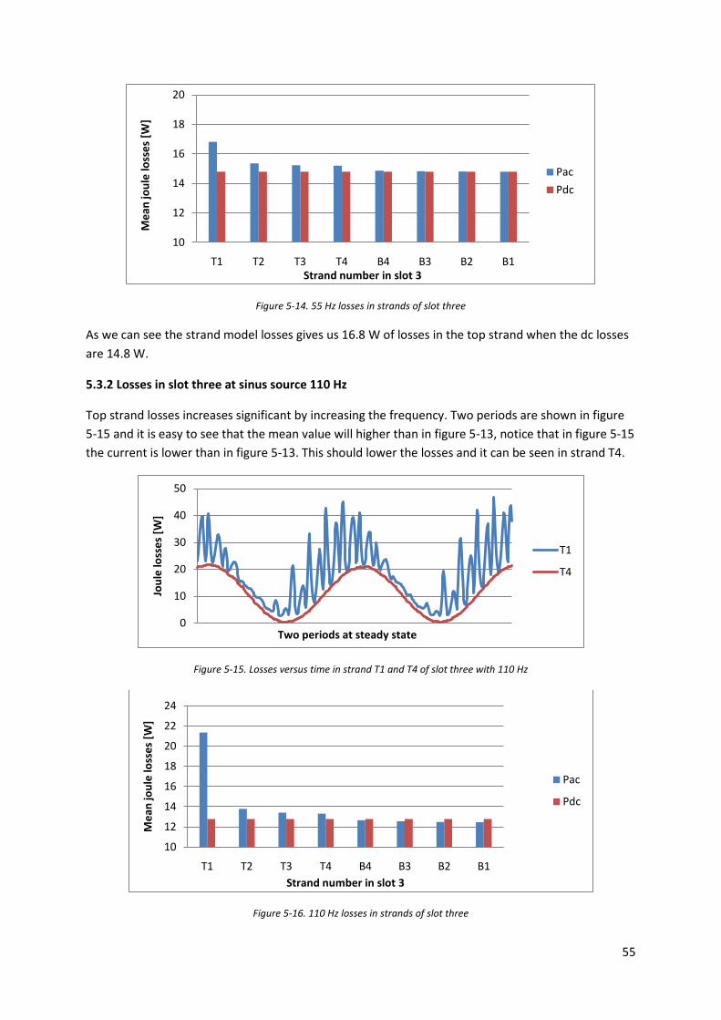
5.3.2 Losses in slot three at sinus source 110 Hz
Top strand losses increases significant by increasing the frequency. Two periods are shown in figure 5-15 and it is easy to see that the mean value will higher than in figure 5-13, notice that in figure 5-15 the current is lower than in figure 5-13. This should lower the losses and it can be seen in strand T4.
Figure 5-15. Losses versus time in strand T1 and T4 of slot three with 110 Hz
Figure 5-16. 110 Hz losses in strands of slot three
10
12
14
16
18
20
T1 T2 T3 T4 B4 B3 B2 B1
Mea
n jo
ule
loss
es [W
]
Strand number in slot 3
Pac
Pdc
0
10
20
30
40
50
Joul
e lo
sses
[W]
Two periods at steady state
T1
T4
10
12
14
16
18
20
22
24
T1 T2 T3 T4 B4 B3 B2 B1
Mea
n jo
ule
loss
es [W
]
Strand number in slot 3
Pac
Pdc

56
As expected the strand model losses gives us higher losses in top strand (21.5 W) when the dc losses (12.8 W) in figure 5-16 are lower due to the lower current.
Figure 5-17. FFT for T1 in slot 3 for both 110 Hz and 55 Hz
5.3.3 Losses in slot three at PWM source 55 Hz
PWM gives a lot of time harmonics with high frequencies and thereby generating even more skin effect losses. By looking at the peak value of T1-losses in figure 5-18 it is easy to understand that PWM really dramatically increases the top strand losses.
Figure 5-18. Losses versus time in strand T1 and T4 of slot 3 with PWM 55 Hz
Figure 5-19. Losses versus time in strand T1 and T4 of slot 3 with PWM 55 Hz
All strands will not generate losses, in figure 5-20 strand in position T2 will not be increased. Figure 5-20 will be the input values in the thermal simulation.
0
5
10
15
20
25
30
1 3 5 7 9 11 13 15 17 19 21 23 25 27 29
Mag
nitd
ude
Joul
e lo
sses
[W]
Nr of harmonic
Sinus 110 Hz
Sinus 55 Hz
0
50
100
150
200
250
Stra
nd Jo
ule
loss
es [W
]
One period during steady state
T1
T4
0
20
40
60
80
1 3 5 7 9 11 13 15 17 19 21 23 25 27 29Mag
nitu
de Jo
ule
loss
es
[W]
Nr of harmonic
T1T4

57
Figure 5-20. 55 Hz PWM losses in strands of slot three
The high frequencies of the PWM voltage source will magnify the joule losses in the strand closest to the air gap. This is again due to the strong frequency dependent phenomena skin and proximity effect. The skin effect ratio in respective strand of slot three is shown in figure 5-21.
Figure 5-21. Skin effect ratio for simulated cases
0
10
20
30
40
50
60
70
T1 T2 T3 T4 B4 B3 B2 B1
Mea
n jo
ule
loss
es [W
]
Position of strand
Pac
Pdc
0,0
0,2
0,4
0,6
0,8
1,0
1,2
1,4
1,6
1,8
1 2 3 4 5 6 7 8
Pac/
Pdc
Strand number in slot 3
55 Hz
110 Hz

58
5.4 Skin effect temperature rises for PWM 55 Hz, sinus 55 Hz and sinus 110 Hz
If skin effect is not taken into account in the thermal design the insulation and surrounding cooling will be under dimensioned. This is the reason for the whole thesis and the temperature rise in conductor slots are the final results.
The aim with the thesis is to find hot spot in conductors.
Figure 5-22. Temperature rise using analytical thermal network with sinusoidal source
Figure 5-23. Temperature rise using FEM thermal model with sinusoidal source
The hotspot is in strand position T1 that have the thermal hotspot. The origin of temperature hotspot is strictly related to the frequency in the voltage source. Knowing where the hotspot is the temperature rise for PWM source can be presented.
0
2
4
6
8
10
12
14
T1 T2 T3 T4 B4 B3 B2 B1
Tem
pera
ture
rise
[Cel
sius
]
Strand in position of slot 3
55 Hz
110 Hz
0
2
4
6
8
10
12
14
T1 T2 T3 T4 B4 B3 B2 B1
Tem
pera
ture
rise
[Cel
sius
]
Strand in position 3
55 Hz
110 Hz

59
Figure 5-24. Temperature rise with PWM 55Hz fundamental
As seen in figure 5-24 the temperature rise in top strand will be around 70 Celsius degrees. By looking at figures 5-22 to 5-24 the conclusion that thermal FEM simulations and the analytical thermal network shows same results with minor deviation.
0
10
20
30
40
50
60
70
80
T1 T2 T3 T4 B4 B3 B2 B1
Tem
pera
ture
rise
[Cel
sius
]
Position of strand
LP-model
FEM

60
6 Conclusion and future work
6.1 Conclusion
To see the current density and copper losses in all strands in a stator slot is really important. In thermal design this is crucial, also for all electrical motor designers the additional losses has to be minimized by mastering these types of losses. Considering skin and proximity effect assuming sinusoidal voltage source the temperature rise in top strand conductor has shown to be very significant. Considering triangular PWM voltage source the temperature in the top strand will be even more significant.
In design of electrical traction motors this phenomena has to be considered in optimization taking the correct strand copper losses into account.
The analytical thermal model is very suitable for thermal temperature rises. The alternative preferred FEM simulation is an easy and fast simulation and agrees with the analytical lumped model.
• The temperature rise in the top strand due to skin- and proximity effect with PWM 55Hz and switching frequency 495 Hz source will be 70 K. For 55 Hz sinusoidal the same parameter will only be 4 K. For higher switching frequencies the temperature will be even higher.
• One of the high magnitude harmonic of PWM 55 Hz will be close to the sum of all 55 Hz sinusoidal non-fundamental harmonics. The rest create a lot of temperature rise in the top strand.
• The tangential component of the flux density in the stator slot will not change raising the frequency from 55 Hz to 110 Hz. Changing from 55 sinusoidal source to PWM 55 Hz source the tangential flux density will increase with 66% in magnitude.
• Flux 2Ds PWM solver is not suitable for copper loss calculations due to the extreme long simulation time. With the latest update of Flux 2D the meshing of the model is even more important due to the long simulation time. In developing of models suitable for skin effect the meshing is decisive for the solution time and it is important to reduce the mesh.

61
6.2 Future work
The two developed models are not perfect due to the time limitation of a master thesis. The conclusions shows the magnitude of impact the skin effect have, due to this the model should be optimized and following future work are presented.
• Study the copper loss harmonics in top strand of order 1-7 and try to reduce them. The reduction can be done both in motor design aspect and in electrical drive control aspect.
• Calculate the skin effect ratio dependent of frequency, many simulations has to be done. This is hopefully done by the future user of this model. Having this information the designers get an overview in how the skin effect PWM losses depends on the frequency, the results has to be compared to analytical formula (2.10) for all simulations.
• Reduce the mesh to one phase to reduce the simulation time of the model.
• The copper resistances are set to a fixed value, with temperature rise there will be a change in resistance using resistivity depending on temperature formula. To make a loop and iterative update the value of the resistance will give losses with high accuracy.
• Study the impact of the number of pulses per period. Using triangular sinus PWM nine pulses per period is a low value in traction application. Increase the switching frequency and study the relation between switching frequency and temperature rises at top strand.
• The losses used in the thermal network are average losses of each strand. To subdivide all strands especially the top strand into sub faces for more realistic input values in the thermal network. This should be applied to both FEM and analytical thermal model.

62
Bibliography [1] Chandur Sadarangani. Electrical Machines – Design and analysis of Induction and Permanent hhhMagnet Motors. Division of Electrical Machines and Power Electronics School of Electrical hhhEngineering (2006)
[2] Stefan Östlund. Elektrisk traktion. Division of Electrical Machines and Power Electronics School of hhhElectrical Engineering (2005)
[3] Fredrik Gustavsson. Elektriska maskiner. Division of Electrical Machines and Power Electronics hhhSchool of Electrical Engineering (1996)
[4] Motor Cad http://www.motor-design.com/ (2012)
[5] Emil Alm. Elektromaskinlära., Asynkronmaskinens teori, driftegenskaper och beräkning, Bd 3,, hhhD.2B (1926)
[6] Cedrat group. Flux 10 – 2D Brushless motor tutorial part 1 and 2 (2008)
[7] Sheppard J.Salon. Finite element analysis of electrical machines. (1995)
[8] Cedrat group. FLUX 2D APPLICATION, Induction motor technical paper. (May 2006)
[9] J Körner. Elektroteknisk handbook band 3, Elektriska maskiner med tillämpningar, Stockholm hhh(1946)
[10] Mohammad Jahirul Islam. Finite-element analysis of eddy currents in the form-wound multi hhhhconductor windings of electrical machines. Helsinki: Helsinki University of Technology
[11] Johan Smeets. Study of turn to turn failure in permanent magnet traction motor for railway hhhhapplications. TRITA-EE 2008:68. Division of Electrical Machines and Power Electronics School of hhhhElectrical Engineering, KTH, Stockholm Sweden, 2008.
[12] Cedrat group. User’s guide vol 1 – General tools, Geometry and mesh. (February 2011)
[13] Jacek F. Gieras. Permanent Magnet Motor Technology: Design and application. Third edition. hhhhISBN 1420064401, 9781420064407 CRC Press, 2009.
[14] Wenliang Chen. Analysis of AC copper losses in form-wound stator winding of high speed hhhhmachines. XR-EE-EME 2010:010. Division of Electrical Machines and Power Electronics School of hhhhElectrical Engineering, KTH, Stockholm Sweden, 2010.
[15] Bo Yang. Development of Thermal Models for Permanent-Magnet Traction Motors. XR-EE-EME hhhh2009:005 Division of Electrical Machines and Power Electronics School of Electrical Engineering, hhhhKTH, Stockholm Sweden, 2009.
[16] Skin effect. http://en.wikipedia.org/wiki/Skin_effect (2012)
[17] Gunnar Kylander. Thermal modeling of small cage induction motors. Doctoral thesis. Department hhhhof Electrical Machines and Power Electronics. CTH, Gothenburg, Sweden, 1995.
[18] Amperes law. http://en.wikipedia.org/wiki/Amp%C3%A8re%27s_circuital_law (2012)

63
[19] S. Iwasaki, Rajesh P. Deodhar. Influence of PWM on the Proximity Loss in Permanent-Magnet hhhhBrushless AC Machines. IEEE TRANSACTIONS ON INDUSTRY APPLICATIONS, VOL. 45, NO. 4, hhhhJULY/AUGUST 2009 [20] Poopak Roshanfekr Fard. ROEBEL WINDINGS FOR HYDRO GENERATORS. Department of Electrical hhhMachines and Power Electronics. CTH, Gothenburg, Sweden, 1995.

64
Appendix A

65
Appendix B

66
Appendix C
Section 1
Section 2
Section 3
1
11 0.5wedge
kapton
HISWRK L BSI
=⋅ ⋅ ⋅
1 1 0.5ins
inskapton
hRK L BSI
=⋅ ⋅ ⋅
11 11 ( 0.5 ( 1 1 ) 1)
2 2
tooth
iron ins
hins HISWR DI DIK L C HSY HISW h L
+=
⋅ ⋅ ⋅ ⋅ + + + + ⋅
s_up1
10.5 1in
kapton
HBRICRK L BCU
=⋅ ⋅ ⋅
s_1
0.000250.5 1in down
kapton
RK L BCU
=⋅ ⋅ ⋅
1( 1 ( 1 1 1))insr
BTRICRKkapton L HSN HBRIC HTRIC
=⋅ ⋅ − −
1
0.5 ( 1 0.00025 1)( (0.5 (( ) ( 1 1 1))))toothup
iron
HCU HBRICRK L C M HSY HISW HSN
⋅ + +=
⋅ ⋅ ⋅ ⋅ + + +
1
0.5 ( 1 0.00025 1)( (0.5 (( 1 1 1 0.00025) )))toothdown
iron
HCU HBRICRK L C HSY HISW HTRIC M
⋅ + +=
⋅ ⋅ ⋅ ⋅ + + − +
1
1
0.5 1 (0.5 1 1)0.5 1
0.5 1 (0.5 1 1)0.5 ( 1 (0.5 1 1))
stbackiron
backtoothiron
DO DI HTRK L BSI
DO DI HTRK L C DO DI HTI
⋅ − ⋅ +=
⋅ ⋅ ⋅⋅ − ⋅ +
=⋅ ⋅ ⋅ ⋅ + ⋅ +

67
Appendix D

68