A previous version of this paper circulated under the title “Some unpleasant properties of loglinearized solutions when the nominal rate is zero.” The authors thank participants from seminars at Australian National University, the Bank of Japan, the Bank of Portugal, the seventh Dynare Conference, the European Central Bank, the Federal Reserve Bank of Atlanta, University of Tokyo, the University of Groningen, the London School of Economics, Vanderbilt University, and the Verein for Sozial Politik for their helpful comments. They also thank Larry Christiano, Isabel Correira, Luca Fornaro, Pedro Teles, and Tao Zha and for their helpful comments. Lena Körber gratefully acknowledges financial support from Cusanuswerk and the Economic and Social Research Council. The views expressed here are the authors’ and not necessarily those of the Federal Reserve Bank of Atlanta or the Federal Reserve System. Any remaining errors are the authors’ responsibility. Please address questions regarding content to R. Anton Braun, Research Department, Federal Reserve Bank of Atlanta, 1000 Peachtree Street, N.E., Atlanta, GA 30309-4470, 404-498-8708, r.anton.braun@atl.frb.org; Lena Mareen Körber, Department of Economics, London School of Economics and Political Science, Houghton Street, London WC2A 2AE, United Kingdom, K, l.m.koerber@lse.ac.uk; or Yuichiro Waki, School of Economics, the University of Queensland, 613 Colin Clark Building (39), QLD 4072, Australia, 61-7-336-56574, y.waki@uq.edu.au. Federal Reserve Bank of Atlanta working papers, including revised versions, are available on the Atlanta Fed’s website at frbatlanta.org/pubs/WP/. Use the WebScriber Service at frbatlanta.org to receive e-mail notifications about new papers.

FEDERAL RESERVE BANK of ATLANTA WORKING PAPER SERIES

Small and Orthodox Fiscal Multipliers at the Zero Lower Bound R. Anton Braun, Lena Mareen Körber, and Yuichiro Waki Working Paper 2013-13 December 2013 Abstract: Does fiscal policy have large and qualitatively different effects on the economy when the nominal interest rate is zero? An emerging consensus in the New Keynesian literature is that the answer is yes. New evidence provided here suggests that the answer is often no. For a broad range of empirically relevant parameterizations of the Rotemberg model of costly price adjustment, the government purchase multiplier is about one or less, and the response of hours to a tax cut is either negative or close to zero. JEL classification: E5, E6 Key words: monetary policy; zero interest rate; fiscal multipliers

1 Introduction

The recent experiences of Japan, the United States, and Europe with zero/near-zero nominalinterest rates have raised new questions about the conduct of monetary and fiscal policy in aliquidity trap. A large and growing body of new research has emerged that provides answersusing New Keynesian (NK) frameworks that explicitly model the zero bound on the nominalinterest rate. The zero bound on the nominal interest rate is particularly important in theNK model because the interest rate policy of the monetary authority plays a central role instabilizing the economy. Very low nominal interest rates constrain the ability of monetarypolicy to respond to shocks and this may result in macroeconomic instability.

One conclusion that has emerged is that fiscal policy has very different effects on theeconomy when the nominal interest rate is zero. Eggertsson (2011) finds that hours workedincrease sharply in response to an increase in the labor tax, a property that he refers to as the“paradox of toil.” Christiano, Eichenbaum, and Rebelo (2011), Woodford (2011) and Ercegand Lindé (2010) find that the size of the government purchase multiplier is close to two oreven larger. These findings stand in stark contrast to the properties of the NK model outsidethe zero bound where the government purchase multiplier is typically about one or less anda higher labor tax has the orthodox property that hours worked fall. The result that fiscalpolicy is most potent in precisely those situations where monetary policy is least effective isa powerful argument for more fiscal stimulus.

New evidence provided in this paper reveals that the properties of fiscal policy in the NKmodel at the zero bound are often not all that different from the properties of fiscal policyaway from the zero bound. We formulate and estimate a tractable model with Rotemberg(1982) costly price adjustment and find that for a broad range of empirically relevant param-eterizations of the model the government purchase multiplier is about 1 or less. Moreover,the response of hours to a higher labor tax is either negative or, when positive, so smallthat the conclusion is that hours are inelastic to change in the labor tax rate. These resultsobtain when parameterizing the model to reproduce either the U.S. Great Recession or theU.S. Great Depression.

Why are our results so different from the previous findings? Focusing on parameterizationsof the model that can reproduce the declines in output and inflation observed during eitherthe U.S. Great Recession or the U.S. Great Depression is important. When this is done,small government purchase multipliers of about one or less and orthodox responses of hoursto an increase in the labor tax are commonplace. We show that these empirical restrictionsimpose tight restrictions on two parameters: the slope of the New Keynesian Philips curveand the expected duration of zero interest rates. This allows us to provide simple intuition

1

for our results that is robust to some of the specific details of our model and to relate ourfindings to previous findings in the literature.

Another reason why our findings are so different pertains to the solution method. Previousresults are based on a solution method that models the nonlinearity induced by the zero boundon the nominal interest rate but that loglinearizes the other equilibrium conditions about astable price level. We show that this solution method can break down in several distinctways when analyzing the zero bound.

One breakdown arises from the fact that the loglinearized solution rules out local dynamicsthat obtain in the true nonlinear model at the zero bound. Perhaps the most significantexample of this point is that the loglinearized solution does not admit conventional responsesof both hours and inflation to a higher labor tax or of both output and inflation to animprovement in technology when the nominal interest rate is zero. We show that the truenonlinear NK model, in contrast, can and does exhibit conventional responses at the zerobound using empirically relevant parameterizations of the model.

Loglinearized solutions can also distort the parameters of the model that are needed tohit a pre-specified set of targets and this in turn can result in distorted inferences about theeffects of fiscal policy. This problem is most severe when parameterizing the model to hittargets from the Great Depression. For instance, we find that the size of the governmentpurchase multiplier drops from 1.8 to 1.2 and that the paradox of toil disappears when weuse an exact solution instead of a loglinearized solution to hit the same targets.

Our analysis does not rule out the possibility of very large fiscal multipliers. Previousresearch by Woodford (2011) and Carlstrom, Fuerst, and Paustian (2012) has found thatfiscal multipliers can exhibit asymptotes at the zero bound using loglinearized solutions. Inthe neighborhood of an asymptote, the response of GDP to a small change in governmentpurchases, for instance, can be arbitrarily large and positive or arbitrarily large and negative.Asymptotes also occur in our nonlinear NK model. They are located in a region of theparameter space that is small but of empirical interest. Depending on the details of thespecification the asymptote occurs when the expected duration of zero interest rates rangesfrom 7 to 25 quarters.

We make these points in a nonlinear stochastic NK model with quadratic price adjust-ment costs as in Rotemberg (1982). Rotemberg costly price adjustment has been used byBenhabib, Schmitt-Grohe, and Uribe (2001) to analyze multiplicity of equilibria due to thezero bound on interest rates; Evans, Guse, and Honkapohja (2008) to model learning in asimilar environment; Aruoba and Schorfheide (2013) to compare zero bound fundamentalsand sunspot equilibria during the Great Recession; Gust, Lopez-Salido, and Smith (2012) to

2

assess the relative importance of demand and technology shocks during the Great Recession;and Eggertsson, Ferrero, and Raffo (2013) to consider the effects of structural reforms ina liquidity trap. Our model also delivers the same loglinearized equilibrium conditions asthe Calvo model with firm specific labor of Eggertsson (2011) and the Calvo model withhomogeneous labor of Woodford (2011).

A distinct advantage of Rotemberg as compared to Calvo price adjustment is tractability.There are no endogenous state variables in our setup and the equilibrium conditions for hoursand inflation can be reduced to two nonlinear equations when the zero bound is binding.These equations are the nonlinear analogues of what Eggertsson and Krugman (2012) referto as “aggregate demand” (AD) and “aggregate supply” (AS) schedules. This structure allowsus to provide intuition for our results and makes it possible to characterize some propertiesof equilibrium analytically. When analytical results are not available, it is straightforward tocompute the various zero bound equilibria by finding the roots of a nonlinear equation in theinflation rate and then checking the other equilibrium conditions. The resulting numericalsolutions are accurate up to the precision of the computer.

Rotemberg costly price adjustment is more tractable than Calvo price setting, yet itis rich enough to capture a common element of both models of price adjustment that isabsent from the loglinearized equilibrium conditions. Both models of costly price adjustmenthave the property that price adjustment absorbs resources whose size changes endogenouslywith the inflation rate. Abstracting from this resource cost has important consequences forthe properties of the model in the zero bound state. For instance, our finding that theloglinearized equilibrium conditions rule out conventional local dynamics that obtain in thetrue model can be attributed to the fact that the resource cost of price adjustment is zero inthe loglinearized solution.

Our research is closest to research by Christiano and Eichenbaum (2012) which is, in part,a response to an earlier version of this paper which demonstrated the possibility of multiplezero bound equilibria. They consider a similar setup to ours and confirm the possibilityof multiple zero bound equilibria. They go on to show that imposing a particular form ofe-learnability rules out one of the two equilibria that occur in their model and find thatthe qualitative properties of the remaining equilibrium are close to the loglinearized solutionunder their baseline parameterization. But the parameterization they consider does notreproduce the declines in output and inflation during the Great Recession documented byChristiano, Eichenbaum, and Rebelo (2011). When we adjust their parameterization to hitthese targets we find that the government purchase multiplier in their favored equilibriumfalls from 2.18 to 1.08. More importantly, our main conclusions about the size and sign of

3

fiscal multipliers do not rely on multiplicity of zero bound equilibrium. In fact, some of ourstrongest results occur in regions of the parameter space where equilibrium is unique. Wealso describe some problems with applying their E-learning equilibrium selection strategy inour setting. It does not omit all forms of multiplicity that we encounter and selects equilibriathat are not empirically relevant while ruling out equilibria that reproduce the data targets.

Our research is also related to but distinct from recent work by Gust, Lopez-Salido, andSmith (2012) and Aruoba and Schorfheide (2013). Gust, Lopez-Salido, and Smith (2012)compare and contrast the role of technology and demand shocks in the Great Recession andfind that demand shocks are more important. Aruoba and Schorfheide (2013) building onprevious work by Mertens and Ravn (2010) contrast the view that the Great Recession wasinduced by an exogenous switch in expectations (a sunspot equilibrium) with an alternativeview that it was driven by shocks to technology, demand and monetary policy. We alsomodel shocks to technology. They make it possible to reconcile parameterizations of themodel that imply a large slope of the New-Keynesian Phillips curve with outcomes fromthe Great Recession and Great Depression. Both events exhibited large output declines butrelatively small declines in the inflation rate. We don’t analyze exogenous sunspot equilibriahere. However, some of the zero bound equilibria that reproduce the Great Recession occurin regions of the parameter space where there is another equilibrium with a positive interestrate. It follows that exogenous sunspot equilibria can be constructed that fluctuate back andforth between positive interest rates and zero interest rates. We also encounter multiple zerobound equilibria which opens the door to a new type of exogenous sunspot equilibrium thatfluctuates between two different zero bound equilibria.

A major advantage of our model is that it is relatively straightforward to determinewhether a nonlinear equation has multiple roots and, if so, how many of those are zerobound equilibria. Ascertaining the presence of multiple equilibria and computing them isa much more challenging task in the versions of the Rotemberg model considered by Gust,Lopez-Salido, and Smith (2012) and Aruoba and Schorfheide (2013) or the model with Calvopricing considered by Fernandez-Villaverde, Gordon, Guerron-Quintana, and Rubio-Ramirez(2012). More generally, our findings of multiple zero bound equilibria, asymptotes in fiscalmultipliers and changes in the model’s local dynamics away from the asymptotes is a matterof some concern because it raises the possibility that these same phenomena are possible inthese other models. Our results offer guidance about the regions of the parameter/shockspace where these issues are most likely to arise.

Finally, our research is related to previous work by Braun and Waki (2010) who find thatthe government purchase multipliers are generally well above one under both Rotemberg and

4

Calvo price setting in a nonlinear perfect nonlinear foresight model with capital accumulation.Their parameterization of the model is not calibrated. One message of our paper is thatgovernment purchase multipliers are much smaller when one uses a parameterization of theNK model that reproduces targets from either the Great Recession or the Great Depression.

The remainder of our analysis proceeds in the following way. In Section 2 we describethe model and equilibrium concept. Then in Section 3 we provide a characterization of zerobound equilibria in the loglinearized economy. Section 4 contains our analytical results forthe nonlinear economy. The parametrization of our model is discussed in Section 5. Sections6 and 7 report numerical results and Section 8 concludes.

2 Model and equilibrium

We consider a stochastic NK model with Rotemberg (1982) quadratic costs of price adjust-ment faced by intermediate goods producers. Monetary policy follows a Taylor rule whenthe nominal interest rate exceeds its lower bound of zero. The equilibrium analyzed here isthe Markov equilibrium proposed by Eggertsson and Woodford (2003).

2.1 The model

Households. The representative household chooses consumption ct, hours ht and bondholdings bt to maximize

E0

∞∑t=0

βt( t∏j=0

dj

){ c1−σt

1− σ− h1+ν

t

1 + ν

}(1)

subject to

bt + ct =bt−1(1 +Rt−1)

1 + πt+ wtht(1− τw,t) + Tt. (2)

The preference discount factor from period t to t+1 is βdt+1, and dt is a preference shock. Weassume that the value of dt+1 is revealed at the beginning of period t. The variable Tt includestransfers from the government and profit distributions from the intermediate producers. Theoptimality conditions for consumption and labor supply choices are

cσt hνt = wt(1− τw,t), (3)

and1 = βdt+1Et

{1 +Rt

1 + πt+1

(ctct+1

)σ}. (4)

5

Final good producers. Perfectly competitive final good firms use a continuum of inter-mediate goods i ∈ [0, 1] to produce a final good with the technology: yt = [

´ 1

0yt(i)

θ−1θ di]

θθ−1 .

The profit maximizing input demands for final goods firms are

yt(i) =

(pt(i)

Pt

)−θyt, (5)

where pt(i) denotes the price of the good produced by firm i and Pt the price of the finalgood. The price of the final good satisfies Pt = [

´ 1

0pt(i)

1−θdi]1/(1−θ).

Intermediate goods producers. Producer of intermediate good i uses labor to produceoutput, using the linear technology: yt(i) = ztht(i), where zt is the common productivity.Labor market is not firm-specific and thus for all firms real marginal cost equals wt/zt.Producer i sets prices to maximize

E0

∞∑t=0

λc,t

[(1 + τs)pt(i)yt(i)− Pt

wtztyt(i)−

γ

2

( pt(i)

pt−1(i)− 1)2Ptyt

]/Pt (6)

subject to the demand function (5). Here λc,t is the stochastic discount factor and is equalto βt(

∏tj=0 dj)c

−σt in equilibrium. We assume that the intermediate goods producers receive

a sales subsidy τs such that (1 + τs)(θ − 1) = θ, i.e. zero profits in the zero inflation steadystate. The last term in the brackets is a quadratic cost of price adjustment. This is assumedto be proportional to the aggregate production yt, so that the share of price adjustment costsin the aggregate production depends only on the inflation rate. The first order condition forthis problem in a symmetric equilibrium is:

0 =wtzt− 1− γ

θπt(1 + πt) + βdt+1Et

{(ctct+1

)σyt+1

yt

γ

θπt+1(1 + πt+1)

}(7)

where πt = Pt/Pt−1 − 1 is the net inflation rate, and we have yt(i) = yt and ht(i) = ht.

Monetary policy. Monetary policy follows a Taylor rule that respects the zero lower boundon the nominal interest rate

Rt = max(0, ret + φππt + φy ˆgdpt), (8)

where ret ≡ 1/(βdt+1)− 1 and ˆgdpt is the log deviation of GDP from its steady state value.1

1The assumption that monetary policy responds directly to variations in dt is made to facilitate comparisonwith other papers in the literature.

6

The aggregate resource constraint is given by

ct = (1− κt − ηt)yt, (9)

where κt ≡ (γ/2)π2t is the resource cost of price adjustment and government purchases

gt = ηtyt. Gross domestic product in our economy, gdpt, is

gdpt ≡ (1− κt)yt = ct + gt. (10)

This definition of GDP assumes that the resource costs of price adjustment are intermediateinputs and are consequently subtracted from gross output when calculating GDP.

The distinction between GDP and output, yt(= ztht), plays a central role in the analysisthat follows. We will show below that loglinearizing equation (10) about a steady state witha stable price level can introduce some large biases when analyzing the properties of thiseconomy in a liquidity trap. To see why this is the case, observe first that GDP falls whenthe term κt increases, even when output is unchanged. It follows that both the sign andmagnitude of movements in GDP can differ from output. However, when equation (10) isloglinearized about a steady state with a stable price level, the term κ disappears, and GDPand output are always equal. In the neighborhood of the steady state, κ is so small that itcan safely be ignored. Ignoring κ is not innocuous if a large shock moves the economy outsideof this neighborhood . One situation where the distinction between GDP and output can beimportant is when one or more shocks drive the nominal interest rate to zero. The distinctionbetween GDP and output is not specific to our model of price adjustment. An analogousterm to κ also appears in the resource contraint under Calvo price setting. In that settingthe term governs the resource cost of price dispersion (see Yun (2005)) and loglinearizingabout a stable price level creates the same type of bias.

2.2 Stochastic equilibrium with zero interest rates

To facilitate comparisons with the previous literature, we consider the Markov equilibriumproposed by Eggertsson and Woodford (2003). The state of the economy st is assumedto follow a two-state, time-homogeneous Markov chain with state space {L,N} (low andnormal) and initial condition s0 = L. Its transition probability from the L state to the Lstate is p < 1 and that from the N state to the N state is 1. We assume that the preferenceshock dt+1, technology shock zt, and fiscal policies (τw,t, ηt) change if and only if st changes:(dt+1, zt, τw,t, ηt) equals (dL, zL, τLw , η

L) when st = L, and (1, z, τw, η) when st = N .We focus exclusively on a Markov equilibrium with state s. Such an equilibrium is char-

7

acterized by two distinct values for prices and quantities: one value obtains when st = L andthe other obtains when st = N . We will use the superscript L to denote the former value andno subscript to indicate the latter value. We assume further that the economy is in a steadystate with zero inflation in the N state, i.e. h = {(1− τw)/(zσ−1(1− η)σ)}1/(σ+ν) and π = 0

if st = N . This implies that in the N state the zero bound doesn’t bind, i.e. it is not the“unintended" zero interest rate steady state in Benhabib, Schmitt-Grohe, and Uribe (2001)and Bullard (2010). When the zero bound binds in the L state, we call such an equilibriuma zero bound equilibrium. We limit attention to situations where this type of equilibriumexists and assume pβdL < 1, to guarantee that utility is finite. Although this structure islimited in the sense that it only has two states, it is rich, for it encapsulates a case withpreference shock only, a case with technology shock only, a case with sunspot shock only((dL, zL, τLw , ηL) = (1, z, τw, η)), and any combinations of these (with perfect correlation).

2.3 Equilibrium hours and inflation in a zero bound equilibrium

An attractive feature of our framework is that the equilibrium conditions for hours and in-flation in the L state can be summarized by two equations in these two variables. Theseequations are nonlinear versions of what Eggertsson and Krugman (2012) refer to as “aggre-gate supply” (AS) and “aggregate demand” (AD) schedules. In what follows, we adopt thesame shorthand when referring to these two equations.

The AS schedule is an equilibrium condition that summarizes intermediate goods firms’price setting decisions, the household’s intratemporal first order condition, and the aggregateresource constraint. To obtain the AS schedule, we start with (7), substitute out the realwage using (3), and then use (9) to replace consumption with hours

0 =(1− κt − ηt)σ

(1− τw,t)z1−σt

hν+σt − 1− γ

θπt(1 + πt) (11)

+ βdt+1Et

{(1− κt − ηt

1− κt+1 − ηt+1

)σ (ztht

zt+1ht+1

)σ−1γ

θπt+1(1 + πt+1)

}.

The AD schedule summarizes the household’s Euler equation and the resource constraint.It is obtained by substituting consumption out of the household’s intertemporal Euler equa-tion (4) using the resource constraint (9). The resulting AD schedule is

1 = βdt+1Et

{1 +Rt

1 + πt+1

((1− κt − ηt)zt

(1− κt+1 − ηt+1)zt+1

)σ (htht+1

)σ}. (12)

8

In a zero bound Markov equilibrium, the AD and AS schedules become

1 = p

(βdL

1 + πL

)+ (1− p)βdL

((1− κL − ηL

)zLhL

(1− η)zh

)σ

(13)

πL(1 + πL) =θ

γ(1− pβdL)

[(1− κL − ηL

)σ(hL)σ+ν

(1− τLw )(zL)1−σ − 1

](14)

where κL = (γ/2)(πL)2 is the price adjustment costs in the L state.2

We have chosen to express the aggregate demand and supply schedules in terms of laborinput rather than GDP. As pointed out above, labor input and GDP can move in independentdirections in our model. Promoting employment is one of the mandates of U.S. monetarypolicy and our choice helps one to understand how labor input responds to fiscal shocks at thezero bound and why it responds in a particular way. For instance, our assumption facilitatesunderstanding when the response of labor input/employment to a change in the labor taxrate is positive and when it is negative and why. This does not mean that GDP is not alsoimportant. For completeness we document properties of both variables when we report ourresults.

3 A characterization of zero bound equilibria and fiscal

multipliers using the loglinearized equilibrium condi-

tions

In this section we show that there are two types of zero bound Markov equilibria using theloglinearized equilibrium conditions and that the fiscal multipliers have different signs andmagnitudes in each type of equilibrium. These results are an important reference point forthe global analysis of the nonlinear model that follows and are also of independent interest.

2Other equilibrium objects are recovered as yL = zLhL, gdpL = (1 − κL)yL, cL =(1− κL − ηL

)yL,

etc. Strictly speaking, not all pairs (hL, πL) that solve this system are equilibria:(1− κL − ηL

)≥ 0 and

reL + φππL + φy y

L ≤ 0 must also be satisfied.

9

3.1 Type 1 and Type 2 equilibria

Following the literature we start by log-linearizing (13) and (14) about the zero inflationsteady state

πL =1− pp

σ[hL + zL

]+

1

p[−reL − (1− p)σ ηL

1− η], (15)

πL =θ(σ + ν)

(1− pβ)γhL +

θ

(1− pβ)γ

[− σ ηL

1− η+

τLw1− τw

− (1− σ)zL], (16)

where we have used the fact that θ = (θ − 1)(1 + τs), and where zL = ln(zL/z), reL =

1/β − 1− dL, ηL = ηL − η and τLw = τLw − τw.3 The other log-linearized equilibrium objectsare given by yL = zL + hL, ˆgdp

L= yL and cL = yL − η/(1 − η) × ηL.4 Observe that the

resource costs of price adjustment have disappeared from the aggregate resource constraint.This property of the loglinearized equilibrium conditions plays a central role in our subsequentanalysis. Another property pertains to the signs of the coefficients on hL in (15) and (16)which we subsequently refer to as slope(AD) and slope(AS). They are both positive. Itfollows that there are two types of zero bound equilibria and neither of them exhibits aconventional configuration of demand and supply. We now provide conditions for each typeof equilibrium. To facilitate the exposition suppose that ηL = τLw = 0.

Proposition 1 Existence of a zero bound equilibrium. Suppose ηL = τLw = 0, (φπ, φy) ≥(p, 0), dL ≥ 0, zL ≤ 0, 0 < p ≤ 1, σ ≥ 1, and that the AD schedule and the AS schedules arenot identical. Then there exists a unique zero bound equilibrium with deflation and depressedlabor input, (πL, hL) < (0, 0), if

1a)(slope(AD)− slope(AS)σ−1

σ+ν

)zL − reL

p> 0 and

1b) slope(AD) > slope(AS),

or

2a)(slope(AD)− slope(AS)σ−1

σ+ν

)zL − reL

p< 0 and

2b) slope(AD) < slope(AS).

If the parameters do not satisfy either both 1a) and 1b) or alternatively both 2a) and 2b),then there is no zero bound equilibrium with depressed labor input hL < 0.5

3Note that ret is the linearized version of reL = 1/(βdL)− 1.4In addition, 1− κL − ηL ≥ 0 and reL + φππ

L + φy yL ≤ 0 must also be satisfied.

5Proofs for this and all other propositions are found in Appendix A.

10

We say that a zero bound equilibrium is of Type 1 when 1a) and 1b) are satisfied, and thatit is of Type 2 when 2a) and 2b) are satisfied. We also refer to configurations of parametersthat satisfy 1a) and 1b) as “Type 1 parameterizatons” and those that satisfy 2a) and 2b) as“Type 2 parameterizations.”

The final statement in Proposition 1 leaves open the possibility that a zero bound equi-librium with hL ≥ 0 exists for parameterizations that satisfy 1a) and 2b) (or 1b) and 2a)).This is a serious possibility because if zL is sufficiently low, labor input will be above itssteady state level in state L. The nominal interest rate could still be zero if there is sufficientdeflation due to high dL and/or GDP is lower than the steady state, i.e. zL + hL < 0.6 Itis our view that zero bound equilibria with high employment and deflation are not relevantfor understanding events such as the U.S. Great Recession or Great Depression. Both eventswere associated with large declines in employment. Proposition 1 tells us that if we limitattention to this type of situation, then all zero bound equilibria are either of Type 1 or Type2.

Most of the recent literature on the zero bound has focused exclusively on Type 1 equi-libria. Type 1 parameterizations have the attractive property that equilibrium is globallyunique (See Proposition 4 in Braun, Körber, and Waki (2012)). A smaller literature in-cluding Bullard (2010), Mertens and Ravn (2010) and Aruoba and Schorfheide (2013) hasconsidered zero bound sunspot equilibria. There is a close relationship between our resultsand this second literature and it is most transparent when zL = 0. Under this assumption, allType 2 equilibria are sunspot equilibria. This is because there is a second equilibrium witha positive nominal interest rate: (hL, πL, RL) = (0, 0, reL). Previous research has focused onpure sunspot equilibria which is a Type 2 equilibrium with dL = 1. By focusing on the Type2 zero bound equilibrium we are implicitly assuming that dL plays two roles: it affects thepreference discount factor and serves as a coordination device for agents beliefs. This is some-times referred to as an endogenous sunspot equilibrium. The exogenous sunspot equilibriaconsidered by Mertens and Ravn (2010) and Aruoba and Schorfheide (2013) set dL = 1 andposit an expectations shock that coordinates expectations on state L.7 Another example ofa Type 2 equilibrium is the deflationary steady-state described in Benhabib, Schmitt-Grohe,and Uribe (2001). Their deflationary steady state is found by setting dL = 1 and p = 1

in equations (16)–(15). The next section shows that the Type 2 equilibrium in our loglin-earized model has the same implications for fiscal policy as the nonlinear sunspot equilibrium

6If it is assumed that zL = 0, then the final clause can be removed and any any ZLB equilibrium mustsatisfy both (1a) and (1b) or both (2a) and (2b). For further details see Braun, Körber, and Waki (2012).

7Aruoba and Schorfheide (2013) also allow for shocks to fundamentals but they are orthogonal to thesunspot shock.

11

considered by Mertens and Ravn (2010). It follows that one important determinant of theproperties of the fiscal multipliers is the parameterization of the model.

3.2 Fiscal policy in the loglinearized model

Fiscal policy has different effects on output and inflation in the two types of equilibria.

Proposition 2 The effects of fiscal policy in the loglinear model

a) In a Type 1 equilibrium, a labor tax increase increases hours and inflation. The gov-ernment purchase output multiplier is above 1.

b) In a Type 2 equilibrium a labor tax increase lowers hours and inflation.

c) Suppose parameters are such that an increase in η results in an increase in governmentpurchases, then in a Type 2 equilibrium the government purchase output multiplier isless than 1.8

4 Analytical results on the global properties of zero bound

equilibria

The local effects of fiscal policy in the nonlinear Rotemberg model also depend on the localslopes of the AS and AD schedules. However, a much richer set of configurations of the ADand AS schedules can be supported as a zero bound equilibrium. In particular, the model canexhibit configurations of AD and AS that are impossible using the loglinearized equilibriumconditions including a conventional configuration with slope(AD) < 0 < slope(AS).

4.1 Slopes of the AS and AD schedules in the nonlinear model

Since the slopes of the AD and AS schedules vary with (hL, πL) in the nonlinear economy, wederive conditions for their local slopes at a given point (hL, πL). Before documenting theseproperties, we wish to remind the reader that we can restrict our attention to the followingrange of πL, since equilibrium consumption and hours must be positive: 1 − κL − ηL > 0,1− pβdL/(1 + πL) > 0, and (1− pβdL)γπL(1 + πL) + θ > 0.

Proposition 3 below establishes a condition under which the nonlinear AD schedule islocally downward sloping.

8In the proof we provide the exact condition in terms of parameters under which an increase in η resultsin an increase in government purchases.

12

Proposition 3 The AD schedule is downward sloping at (hL, πL) if and only if

1

σ

pβdL/(1 + πL)2

1− pβdL/(1 + πL)+

(κL)′

1− κL − ηL< 0, (17)

where (κL)′ = γπL. It is upward-sloping (vertical) if and only if the left hand side is positive(zero).

To understand these results, recall that the AD schedule is obtained by combining theEuler equation and the aggregate resource constraint. The Euler equation, in isolation,creates a positive relationship between inflation and consumption because higher (expected)inflation lowers the real interest rate. In the true model this gets balanced against theaggregate resource constraint, which creates a negative relationship between inflation andthe hours-consumption ratio when the inflation rate is negative. An increase in inflationreduces the resource costs of price adjustment, thereby reducing the gap between hours andconsumption. Loglinearizing the aggregate resource constraint at π = 0 loses this secondchannel. The hours-consumption ratio becomes independent of inflation in the aggregateresource constraint and the slope of the AD schedule is unambiguously positive. Observenext that the first term in (17) is the inflation elasticity of consumption implied by the Eulerequation and the second term is the inflation elasticity of the hours-consumption ratio impliedby the aggregate resource constraint. Since h = c× (h/c), their sum is the inflation elasticityof hours, and its reciprocal is naturally the local slope of the AD schedule. The first term isalways non-negative, and the second term is negative when πL < 0. Loglinearizing about astable price level imposes (κL)′ = κL = 0 and the second term disappears from (17). Thus,the presence of price adjustment costs in the aggregate resource constraint is responsible forthe possibility of a downward sloping AD schedule in the nonlinear model.

Using these results we can document one breakdown in the loglinearized solution. Supposep = 0 and πL < 0. Under these assumptions the slope of the AD schedule is unambiguouslynegative. The loglinearized equilibrium, in contrast, has the property that all zero boundequilibria have a positively sloped AD schedule. This breakdown occurs in any zero boundequilibrium and does not depend on the size of the shocks beyond the requirement that theybe large enough to induce a zero nominal interest rate. We will show in the numerical resultsthat follow that this type of breakdown can occur for values of p that are as large as 0.86and that it has direct implications for the sign of the response of hours to a change in thetax rate.

The next proposition characterizes the local slope of the AS schedule.

13

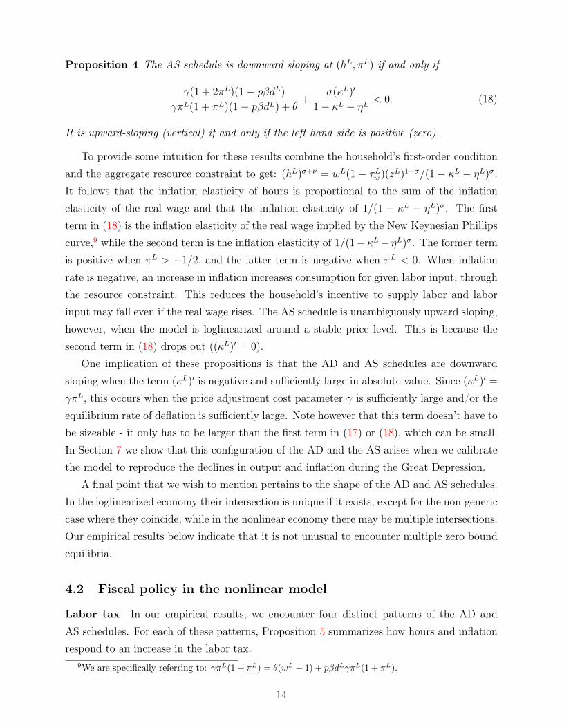
Proposition 4 The AS schedule is downward sloping at (hL, πL) if and only if

γ(1 + 2πL)(1− pβdL)

γπL(1 + πL)(1− pβdL) + θ+

σ(κL)′

1− κL − ηL< 0. (18)

It is upward-sloping (vertical) if and only if the left hand side is positive (zero).

To provide some intuition for these results combine the household’s first-order conditionand the aggregate resource constraint to get: (hL)σ+ν = wL(1− τLw )(zL)1−σ/(1− κL − ηL)σ.It follows that the inflation elasticity of hours is proportional to the sum of the inflationelasticity of the real wage and that the inflation elasticity of 1/(1 − κL − ηL)σ. The firstterm in (18) is the inflation elasticity of the real wage implied by the New Keynesian Phillipscurve,9 while the second term is the inflation elasticity of 1/(1−κL− ηL)σ. The former termis positive when πL > −1/2, and the latter term is negative when πL < 0. When inflationrate is negative, an increase in inflation increases consumption for given labor input, throughthe resource constraint. This reduces the household’s incentive to supply labor and laborinput may fall even if the real wage rises. The AS schedule is unambiguously upward sloping,however, when the model is loglinearized around a stable price level. This is because thesecond term in (18) drops out ((κL)′ = 0).

One implication of these propositions is that the AD and AS schedules are downwardsloping when the term (κL)′ is negative and sufficiently large in absolute value. Since (κL)′ =

γπL, this occurs when the price adjustment cost parameter γ is sufficiently large and/or theequilibrium rate of deflation is sufficiently large. Note however that this term doesn’t have tobe sizeable - it only has to be larger than the first term in (17) or (18), which can be small.In Section 7 we show that this configuration of the AD and the AS arises when we calibratethe model to reproduce the declines in output and inflation during the Great Depression.

A final point that we wish to mention pertains to the shape of the AD and AS schedules.In the loglinearized economy their intersection is unique if it exists, except for the non-genericcase where they coincide, while in the nonlinear economy there may be multiple intersections.Our empirical results below indicate that it is not unusual to encounter multiple zero boundequilibria.

4.2 Fiscal policy in the nonlinear model

Labor tax In our empirical results, we encounter four distinct patterns of the AD andAS schedules. For each of these patterns, Proposition 5 summarizes how hours and inflationrespond to an increase in the labor tax.

9We are specifically referring to: γπL(1 + πL) = θ(wL − 1) + pβdLγπL(1 + πL).

14

Proposition 5 Response of hours and inflation to a change in the labor tax

a) If both the AS and AD schedule is downward sloping and the AS schedule is steeper orif the AS schedule is upward sloping and the AD schedule is downward sloping, then ahigher labor tax lowers hours and rises inflation.

b) If both the AS and the AD schedule are upward sloping and the AD schedule is steeper,then a higher labor tax increase rises hours and inflation. Consumption also increasesif πL < 0.

c) If both the AS and the AD schedule are upward sloping and the AS schedule is steeper,then a higher labor tax lowers hours and inflation. Consumption also falls if πL < 0.

Case a) is unique to the nonlinear model. Moreover, it implies a conventional response ofhours to labor income tax; hours fall in response to a labor tax increase. Cases b) and c) aregeneralizations of Proposition 2 a) and b).

Government spending multiplier We have explored the possibility of deriving analyticalresponses in the nonlinear economy and found that the magnitude of the response of GDP andother variables to a change in government purchases is difficult to pin down in the nonlineareconomy. Instead we will use numerical solutions to investigate this question which requiresus to assign particular values to the model’s parameters.

5 Parameterization of the model

We divide this discussion into two parts. We start by describing how we assign values to theparameters that are not specific to the zero bond. Then we discuss how we assign values toparameters that pertain to the zero bound.

5.1 Parameters that are not specific to the zero bound

We will demonstrate that some of the properties of the model can be linked to the size ofthe slope of the conventional loglinear New Keynesian Phillips Curve (NKPC). In our modelthis coefficient is given by slope(NKPC) ≡ θ(σ + ν)/γ. There are many different choices ofparameters that can make this number big or small. Here we describe how we come up withreference values for these parameters that are used to produce our baseline results.

Our reference value of σ is one. This corresponds to the case of log preferences overconsumption, which is a common reference point in the DSGE literature. The parameter θ

15

is set to 7.67, which implies a markup of 15%. We found that θ and γ are not individuallyidentified by our estimation procedure. Given the central role played by γ in the NK model,we decided to fix θ and estimate γ. Our choice of θ lies midway between previous estimatesfrom disaggregated and aggregate data. Broda and Weinstein (2004) find that the medianvalue of this parameter ranges from 3 to 4.3 using 4-digit level industry level data for alter-native country pairs. Denes, Eggertsson, and Gilbukh (2013) estimate θ to be about 13 in arepresentative agent NK model. It is also well known that β is not well identified in DSGEmodels. Consequently, β is fixed at 0.997 which implies an annual preference rate of timepreference of 1.2%.

We also fix the government purchase share parameter η at 0.2 and the labor tax τw at0.2. The remaining two parameters ν and γ are estimated using a strategy that is similar tothe one used by policy institutions such as the Bank of England. They estimate structuralparameters via Bayesian MLE over a sample period that ends before the nominal interest ratefalls to zero (see e.g. Burgess, Fernandez-Corugedo, Groth, Harrison, Monti, Theodoridis,and Waldron (2013)). We estimate ν and γ via Bayesian MLE using quarterly U.S. dataon inflation, the output gap and the Federal Funds rate over a sample period that extendsfrom 1985:I through 2007:IV.10 Complete details on our estimation procedure are reportedin the Online Appendix.11 Here we briefly comment on the resulting estimates of γ and ν.The estimated posterior mode of γ is 458.4 and 90% of its posterior mass lies between 315and 714. This value is larger than Ireland (2003) who estimates a value of 162, and Gust,Lopez-Salido, and Smith (2012) who estimate γ = 94. If we use a tighter prior on γ, we canproduce estimates of γ that lie in the range of 100 to 150. However, most posterior mass iscentered well outside of the prior. Relaxing the prior on this parameter yields diagnosticsthat suggest that the resulting estimates are less influenced by the prior in the sense thatthere is more overlap of the prior and posterior densities for γ and by the fact that the peaksof the likelihood function and posterior mode are close. The posterior mode for ν, whichgoverns the curvature of the disutility of work, is 0.28 with 90% of its posterior mass lying inthe interval 0.08 and 0.63. A complete set of estimation results including priors is provided inthe Online Appendix. These estimates in conjunction with our choices for θ and σ imply thatslope(NKPC) = 0.0214 which is very close to the value of 0.024 estimated by Rotembergand Woodford (1997).

10Our measure of the output gap uses the Congressional Budget Office measure of potential GDP.11The Online Appendix is available at: https://sites.google.com/site/yuichirowaki/research.

16

5.2 Parameters and shocks that are specific to the zero bound

We consider two specific episodes with zero interest rates: the U.S. Great Recession (GR)and the U.S. Great Depression (GD). To facilitate a comparison of our results with those inthe previous literature, we consider the two state Markov zero bound equilibria we describedin Section 2.2. This structure also allows us to provide a transparent and intuitive analysisof our results, and to identify the possibility of multiple equilibria. To pursue this strategy,we need to specify p, which determines the expected duration of zero interest rates, and thesize of the shocks that produce a zero nominal interest rate. Rather than using a specific p,we report results for a range of values of p. For each given value of p, we choose dL and zL

to reproduce targeted declines on output and the annualized inflation rate, assuming thatthe fiscal policy in the L state is the same as in the steady state, i.e. (τLw , η

L) = (τw, η).The Online Appendix explains how these targets uniquely pin down dL and zL. We thenmeasure the fiscal policy effects by computing how an equilibrium in the L state changeswhen (τLw , η

L) changes from (τw, η).Our targets for the GR are taken from Christiano, Eichenbaum, and Rebelo (2011).

They provide empirical evidence that the U.S. financial crisis that ensued after the collapseof Lehman Brothers in the third quarter of 2008 produced a peak decline in GDP of 7% anda peak decline in the inflation rate of 1%. The GD targets are taken from Eggertsson (2011)who posits a 30% decline in GDP and a 10% decline in the annualized inflation rate.

6 Numerical results for the Great Recession

In this section we describe the fiscal multipliers that emerge from our model using our esti-mated parameterization and the GR targets. We then relate our findings to other results inthe literature.

6.1 Our results

Fiscal multipliers are reported in Figure 1 for alternative values of p that range from 0.05

to 0.95. For each choice of p the shocks to dL and zL have been adjusted so that themodel produces a 7% decline in output and a 1% decline in the inflation rate. Figure 1is divided into three panels. The upper and middle panels display the responses of GDPand hours respectively to a one unit change in government purchases. The lower panelshows the response of hours in percentage points to a one percentage point increase in thelabour tax. Each panel reports results for three subintervals p ∈ [0.05, 0.8], p ∈ [0.8, 0.86]

17

and p ∈ [0.865, 0.95]. Results using the exact nonlinear solution of the model are labeled asNL and results using the loglinearized solution are labeled as LL. In some cases there aretwo nonlinear zero bound equilibria. The label “NL (target)" refers to the equilibrium thatreproduces the calibration targets, while “NL (non-target)" refers to the nonlinear equilibriumthat doesn’t hit the targets.

One of the main objectives of this paper is to demonstrate that there are a broad rangeof empirically plausible parameterizations of the NK model that deliver small governmentpurchase multipliers at the zero bound. Figure 1 shows that the government purchase mul-tipliers are small over two distinct intervals of p. Results in the leftmost chart of this figureindicate that the government purchase GDP multiplier is smaller than 1.15 when p ≤ 0.8.It ranges from a high of 1.14 when p = 0.8 to a low of 1.00 when p = 0.05. The governmentpurchase hours multiplier has a similar pattern. It falls from 1.15 to 0.95 as p is reducedfrom 0.8 to 0.05. From the rightmost charts of Figure 1, one can see that the governmentpurchase multiplier is also small when p ≥ 0.88 in the NL (targeted) equilibrium. In thisinterval the responses of GDP and hours to a one unit change in government purchases areboth less than one. For instance, when p = 0.9 the value of the government purchase GDPmultiplier is 0.62 and the hours multiplier is 0.72 and when p = 0.95, the two multipliers arerespectively 0.79 and 0.86.

Figure 1 also reports response of hours in percentage points to a one percentage pointincrease in the labor tax. It shows that the sign of the labor tax hours multiplier is orthodoxin two distinct regions. Hours fall in response to an increase in the labor tax when p < 0.6 andwhen p ≥ 0.865. Even when the response of hours to a tax increase is positive, its magnitudeis generally very small. The labor tax multiplier never exceeds 0.2% when p < 0.75. whichwe interpret to mean that hours worked are highly inelastic to changes in the labor tax.

There are two qualifications to these results. The first qualification is clearest in themiddle and right charts of Figure 1. At a value of p ≈ 0.86 the fiscal multipliers havean asymptote. In the neighborhood of the asymptote the fiscal multipliers become verylarge and their signs flip on either side of the asymptote. Woodford (2011) and Carlstrom,Fuerst, and Paustian (2012) have previously documented asymptotes in fiscal multipliersusing loglinearized solutions. Our results indicate that they also arise in nonlinear NK models.The second qualification can be seen in the right panels of Figure 1. When p ∈ [0.87, 0.89],there is a second zero bound equilibrium of the model. This equilibrium is not targeted andfor most values of p it produces responses of inflation and/or output that are very far fromthe targets. The non-targeted zero bound equilibrium also occurs in a very small interval tothe left of the asymptote.

18

A disturbing aspect of our results is that the asymptote occurs at a value of p that is closeto values maintained in previous research. Denes, Eggertsson, and Gilbukh (2013) report anestimate of p = 0.86 and Christiano and Eichenbaum (2012) posit a value of p = 0.775. Smallperturbations of p in this region have large effects on the magnitudes and/or signs of thefiscal policy multipliers.

High values of p > 0.9, which imply expected durations of zero interest rates that exceed 10quarters, are most consistent with the long episodes of nearly zero interest rates experiencedby the U.S., some European countries and Japan ( See rightmost charts in Figure 1 ). Forinstance, the U.S. and Japan have experienced interest rates that are close to zero since thefourth quarter of 2008.12

Figure 1 also reports fiscal multipliers computed from the loglinearized solution. Forp ≥ 0.865, the linear structure of this solution implies that it cannot discover the presenceof the other zero bound equilibrium. When p ≥ 0.9, there is a single zero bound equilibriumin the true model and the loglinear solution approximates this solution well. Both solutionshave the properties that the government purchase GDP is less than one and that hours fallin response to an increase in the labor tax. A range of NK models including models withCalvo pricing have the same loglinear structure as our model. If the loglinear solution worksas well in these other models as it does here, then these results for p ≥ 0.9 also obtain in alarger class of NK models.

Biases in the government purchase multiplier are somewhat larger for values of p thatare to the left of the asymptote. For instance, when p < 0.4 the government purchase GDPmultiplier is less than one using the loglinearized solution but slightly above one using theexact solution. Biases for the labor tax multiplier are larger too. For values of p ≤ 0.57 theloglinearized solution predicts that the response of hours to a tax increase is positive whenin fact it is negative.

The largest biases occur in the neighborhood of the asymptote. The loglinearized solutionunderstates the true multipliers for GDP, hours and inflation immediately to the left of theasymptote and overstates the size of these multipliers just to the right of the asymptote.

Table 1 reports other properties of the model for selected values of p that help providemore intuition for our results. It is immediately clear from inspection of the table thatthe asymptote occurs at a point where the slopes of the AD and AS schedules are parallel.To the right of the asymptote, the targeted nonlinear equilibrium has the property thatslope(AS) > slope(AD) > 0 and it follows immediately from Proposition 5 that the sign ofthe labor tax multiplier must be negative. The loglinearized solution is consistent with this

12 Hayashi and Koeda (2013) who identify two other episodes with low interest rates: March 1999 – July2000 and March 2001 – June 2006.

19

property of the model since it produces a Type 2 equilibrium. Immediately to the left of theasymptote, both solutions have the property that slope(AD) > slope(AS) > 0 and there isa paradox of toil.

We have seen that the Rotemberg model has a second zero bound equilibrium to the rightof the asymptote. The properties of this second equilibrium vary with the value of p. It hasthe property that slope(AS) < slope(AD) < 0 when p ∈ [0.867, 0.89] and 0 < slope(AS) <

slope(AD) when p ∈ [0.86, 0.865].

In Section 3.1, we discussed the possibility of multiple equilibria and sunspot equilibriawhen the loglinearized solution is a Type 2 equilibrium. Table 1 indicates that the loglin-earized solution is a Type 2 equilibrium when p = 0.9. In fact, the equilibrium is Type 2when p ≥ 0.865. In this region there are two indeed equilibria. One equilibrium is the zerobound equilibrium displayed in Figure 1 and the other equilibrium has a positive interestrate, a positive inflation rate and high hours worked. In the positive interest rate equilib-rium, the government purchase multiplier is less than one and hours fall in response to alabor tax increase since slope(AD) < 0 < slope(AS). The true model also has a positiveinterest rate equilibrium when p ≥ 0.86 and inflation and hours are also above their steady-state values in this equilibrium. The government purchase multiplier is less than one butslope(AD) > slope(AS) > 0 and the response of hours to a tax increase is positive.

Given that there are multiple equilibria, if the intent is to select the equilibrium thatreproduces the GR targets, then the shocks to fundamentals must also act to coordinatebeliefs on that equilibrium. In this sense the (targeted) zero bound equilibrium is a typeof endogenous sunspot equilibrium. We do not pursue this possibility here but one couldconstruct other sunspot equilibria that alternate from positive interest rates to zero interestrates as in Mertens and Ravn (2010) or Aruoba and Schorfheide (2013). When p ∈ [0.86, 0.89],it is also possible to entertain sunspot equilibria that switch between the two zero boundequilibria with distinct local dynamics and an equilibrium with a positive interest rate.

Christiano and Eichenbaum (2012) have proposed that one use an E-learning criteria torule out multiple zero bound equilibria in nonlinear NK models. Applying that criterion heredoes not resolve the issue of multiplicity of equilibrium for p ∈ [0.86, 0.865] in our nonlinearmodel. This is because both the positive interest rate equilibrium and the non-targeted zerobound equilibrium are E-learnable. More importantly, neither of these equilibria reproducethe GR targets. For instance, the E-learnable zero bound equilibrium produces a 13% declinein GDP and an annualized rate of deflation of 5% when p = 0.865 and the positive interestrate equilibrium has the property that GDP falls but only by 0.6%. Hours, in contrast, are 5%above their steady state level. When p exceeds 0.865, the E-learning criterion rules out all zero

20

bound equilibria in the Rotemberg model and selects the positive interest rate equilibrium.However, the positive interest rate equilibrium continues to predict a GDP response of aboutzero. Moreover, hours are even higher and increase with p. We do not believe that it is usefulto use an equilibrium selection criterion that rejects zero bound equilibria that exceed sevenquarters and reproduce the GR facts and instead selects equilibria that are inconsistent withthe fact that the U.S. Great Recession has been accompanied by zero nominal interest rates,depressed GDP, depressed hours and a depressed inflation rate.

Next consider results in Table 1 for p ≤ 0.8. In Figure 1, we documented a paradox of toilusing the loglinearized solution and an orthodox response of hours using the exact solutionwhen p ≤ 0.57. A possible explanation for this finding was provided in Section 4.1 where wefound that the loglinearized solution produces the wrong slope of the AD schedule in anyzero bound equilibrium when p is in the neighborhood of zero. It was not possible, however,to establish the size of this neighborhood using analytical arguments. Results in Table 1indicate that this neighborhood can be very large. For instance, when p = 0.5, the slopesof AD and AS have their conventional signs in the Rotemberg model which in turn impliesfrom Proposition 5 that there is no paradox of toil. The slope of the AD schedule using theloglinearized solution is positive and exceeds the slope of the AS schedule. This is why theloglinearized solution incorrectly predicts a paradox of toil in this region of the parameterspace. More generally, the two solutions are different when p ≤ 0.57 or in words when theexpected duration of zero interest rates is less than two quarters.

The evidence we discussed above suggests that two quarters is a very short expectedduration of zero interest rates. However, short expected durations cannot be completely ruledout on a priori grounds. Short expected durations of zero interest rates occur in empiricalanalyses of the zero bound such as Aruoba and Schorfheide (2013) which require a longsequence of negative monetary policy shocks to account for the fact that the U.S. policy ratehas been about zero since 2008. It is also not difficult to find alternative parameterizationsof the model that hit the GR targets and where this same type of breakdown occurs withhigher values of p. We will present results for another parameterization below where the truemodel produces a conventional configuration of AD and AS for p as large as 0.857.

Table 1 also reports the resource cost of price adjustment expressed as a ratio of output.The magnitude of the price adjustment cost in the Rotemberg model is 0.14% of output orless for all equilibria that reproduce the GR targets. It is difficult to directly measure theoverall magnitude of the resource cost of price adjustment but a rough idea of the potentialmagnitude of this cost is provided by Levy, Bergen, Dutta, and Venable (1997) who find thatmenu costs constitute 0.7% of revenues of supermarket chains.

21

Recognizing the resource cost of price adjustment plays a central role in obtaining aconventional configuration of the slopes of AD and AS. Our analytical results in Section4 offered some insight into their role. Another way to understand the role of the resourcecost of price adjustment is to observe that if it was absent, the response of hours and GDPwould be identical. Thus, evidence that hours and GDP are responding differently to a shockillustrates that resource costs matter. This is the case for p ∈ [0.215, 0.57].13 In this intervalhigher labor taxes reduce hours and increase GDP. It follows that the positive response ofGDP stems from the fact that the reduction in resource costs is larger than the decline inhours.

6.2 Relating our results to the literature

We now consider how our results relate to the literature which has found that governmentpurchase GDP multipliers are large and positive and that hours fall in response to a taxcut when the interest rate is zero. This discussion also provides us with an opportunity todocument the robustness of our conclusions to the parameterization of the model. In whatfollows we will consider parameterizations in which the value of γ is as low as 100, values ofθ that range from one to 13 and a value of ν that is as high as 1.69.

6.2.1 Differences in the shocks: Preference shock only

Following Eggertsson and Woodford (2003), many analyses of the zero bound consider sce-narios where a single demand shock drives the nominal interest rate to zero. One possibleexplanation for the difference between our results and these previous results is that we allowtwo shocks to do this. We now adopt their assumption and set zL = z = 1. With a singleshock it is no longer possible to hit both Great Recession targets for general p, and we needto adjust one or more parameters from their baseline values. We choose to adjust θ and keepthe other parameters fixed.14

Fiscal multipliers using the exact and loglinearized solutions are reported in Figure 2 forvalues of p that range from 0.05 to 0.95. Other properties of the model are reported forselected values of p in Table 2.

Observe that the GDP multiplier is now less than 1.1 when p ≤ 0.9. Most empiricalevidence suggests that θ ≥ 2 (see e.g. Broda and Weinstein (2004)). If we limit attentionto values of θ ≥ 2 and thus p ≤ 0.84, the government purchase GDP multiplier is 1.04 orless and the labor tax multiplier is 0.18 or less. Note further that for values of p ≤ 0.9, the

13The GDP response to a higher labor tax are reported in our Online Appendix.14The Online Appendix describes how dL and θ are calibrated to hit the two GR targets.

22

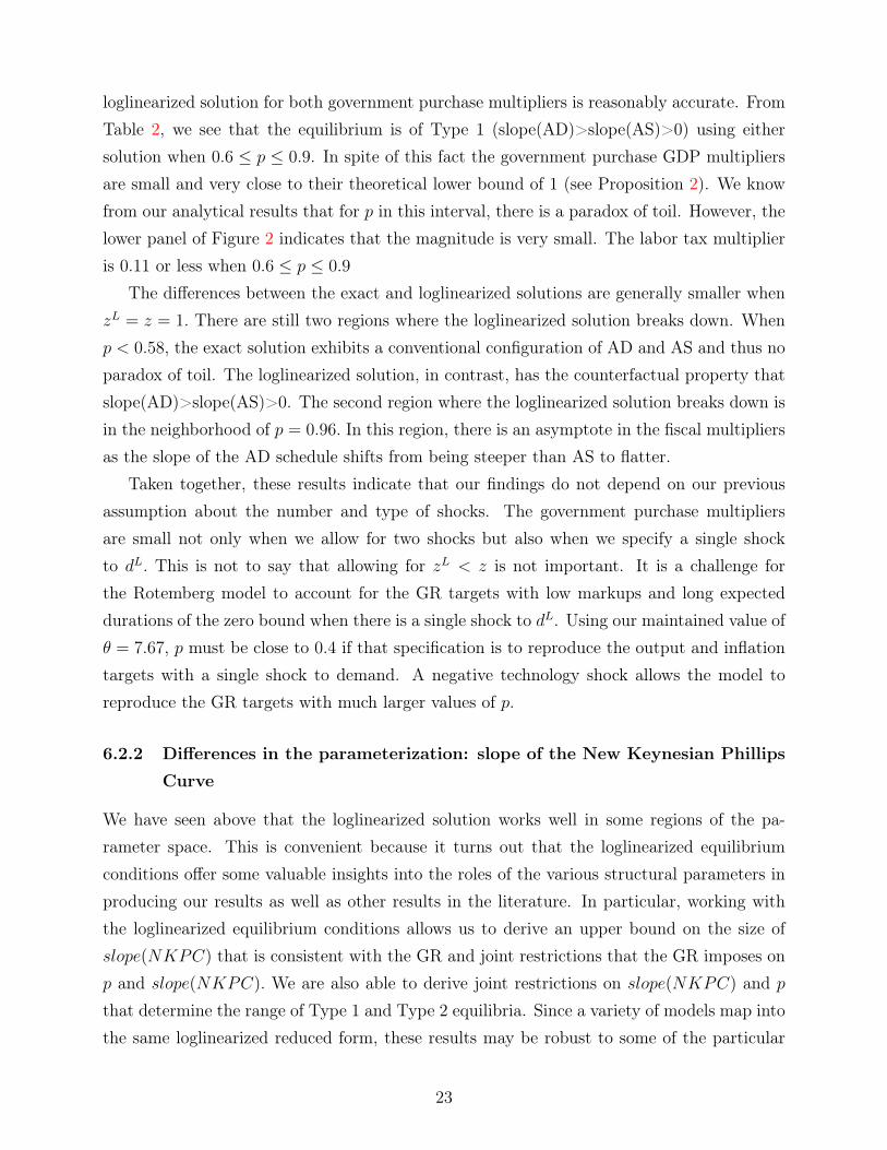
loglinearized solution for both government purchase multipliers is reasonably accurate. FromTable 2, we see that the equilibrium is of Type 1 (slope(AD)>slope(AS)>0) using eithersolution when 0.6 ≤ p ≤ 0.9. In spite of this fact the government purchase GDP multipliersare small and very close to their theoretical lower bound of 1 (see Proposition 2). We knowfrom our analytical results that for p in this interval, there is a paradox of toil. However, thelower panel of Figure 2 indicates that the magnitude is very small. The labor tax multiplieris 0.11 or less when 0.6 ≤ p ≤ 0.9

The differences between the exact and loglinearized solutions are generally smaller whenzL = z = 1. There are still two regions where the loglinearized solution breaks down. Whenp < 0.58, the exact solution exhibits a conventional configuration of AD and AS and thus noparadox of toil. The loglinearized solution, in contrast, has the counterfactual property thatslope(AD)>slope(AS)>0. The second region where the loglinearized solution breaks down isin the neighborhood of p = 0.96. In this region, there is an asymptote in the fiscal multipliersas the slope of the AD schedule shifts from being steeper than AS to flatter.

Taken together, these results indicate that our findings do not depend on our previousassumption about the number and type of shocks. The government purchase multipliersare small not only when we allow for two shocks but also when we specify a single shockto dL. This is not to say that allowing for zL < z is not important. It is a challenge forthe Rotemberg model to account for the GR targets with low markups and long expecteddurations of the zero bound when there is a single shock to dL. Using our maintained value ofθ = 7.67, p must be close to 0.4 if that specification is to reproduce the output and inflationtargets with a single shock to demand. A negative technology shock allows the model toreproduce the GR targets with much larger values of p.

6.2.2 Differences in the parameterization: slope of the New Keynesian Phillips

Curve

We have seen above that the loglinearized solution works well in some regions of the pa-rameter space. This is convenient because it turns out that the loglinearized equilibriumconditions offer some valuable insights into the roles of the various structural parameters inproducing our results as well as other results in the literature. In particular, working withthe loglinearized equilibrium conditions allows us to derive an upper bound on the size ofslope(NKPC) that is consistent with the GR and joint restrictions that the GR imposes onp and slope(NKPC). We are also able to derive joint restrictions on slope(NKPC) and pthat determine the range of Type 1 and Type 2 equilibria. Since a variety of models map intothe same loglinearized reduced form, these results may be robust to some of the particular

23

modeling assumptions that we have made.We first show how our GR targets restrict the plausible range of slope(NKPC). For

expositional purposes, suppose that the only shock that induces the nominal rate to fall tozero is a discount factor shock.15 Then it follows from the loglinearized AS equation (16)that

1− βp = slope(NKPC)hL

πL(19)

Next observe that our GR targets imply hL/πL = (−0.07)/(−0.0025) ≈ 28 when zL = 0.Combining these two pieces of information and setting p = 0 implies that the largest valueof slope(NKPC) that is consistent with the GR targets is 1/28 ≈ 0.036.

More generally, equation (19) shows that reproducing the GR imposes joint restrictionson p and slope(NKPC). These restrictions have some empirical content. For instance, if oneconditions on a value of slope(NKPC) ≈ 0.02, which is the value implied by our estimates,then p ≈ 0.4. Entertaining a value of p ≥ 0.9 requires that slope(NKPC) = θ(σ + ν)/γ ≤0.005. In the preference-shock-only case, we accomplished this by lowering θ.16

The loglinearized model can also be used to relate the conditions for Type 1 and Type 2zero bound equilibria to the values of slope(NKPC). Depending on whether the left handside of

(1− p)(1− pβ)

pRslope(NKPC)

σ(20)

is larger/smaller than the right hand side, the AD schedule is steeper/flatter than the ASschedule. The left hand side of equation (20) is declining in p. An implication of this conditionis that producing a Type 1 zero bound equilibrium when p is large requires a very small valueof slope(NKPC)/σ. For instance, using our reference parameterization (σ = 1 and β ≈ 1)producing a type 1 equilibrium with p > 0.9 requires that slope(NKPC) < 0.011.

More generally, if the objective is to produce a large region where the equilibrium is ofType 1, then very small values of slope(NKPC) and/or small values of p are desirable. Asmall value of slope(NKPC) is associated with a large value of γ or alternatively small valuesof θ, σ and/or ν. To make the range of Type 2 equilibria large instead, it is desirable to useconfigurations that make slope(NKPC) large and/or p large.

These results imply that the parameters p, θ, σ, ν and γ are of particular significance. In15We discuss the role of technology shocks in the Online Appendix.16 We show in the Online Appendix that a negative technology shock increases the value of p implied by (16)

for given slope(NKPC), and that is why we are able to hit the GR target without lowering slope(NKPC)in that specification.

24

what follows, we will focus on particular combinations of these parameters that have beenused in the previous literature.

6.2.3 Accounting for the Great Recession with the parameterization of Chris-

tiano and Eichenbaum (2012)

We next turn to conduct a more detailed comparison of our results with those of Christianoand Eichenbaum (2012). They find that the government purchase multiplier exceeds 2 in anonlinear Rotemberg model that is very close to ours.17 Following their paper, we set thepreference discount factor β = 0.99, the coefficient of relative risk aversion for consumptionσ = 1 and the curvature parameter for leisure ν = 1. The technology parameter θ thatgoverns the substitutability of different types of goods is set to three, the adjustment costs ofprice adjustment γ = 100, and the conditional probability of exiting the low state p = 0.775.

Our model has three fiscal parameters. The labor tax τw = 0.2, government purchases sharein output η = 0.2, and the subsidy to intermediate goods producers τs is set so that steady-state profits are zero. Finally, the coefficients on the Taylor rule are φ = 1.5 and φy = 0. Withthis parameterization our loglinearized system is identical to the one reported in Christianoand Eichenbaum (2012).18

Row 1 of Table 3 reproduces their baseline results using our nonlinear model and theloglinearized solution.19 The loglinear solution yields a government purchase multiplier of2.77 implying that fiscal stimulus is highly effective at the zero bound. Note next that thereis a paradox of toil. This follows from the observation that the equilibrium is of Type 1. Themagnitude is very large with hours increasing by 4.84% to a one percentage point increasein the labor tax. For purposes of comparison, it is about five times as large as the responsereported in Eggertsson (2011) for a similar model that is estimated to hit targets from theGreat Depression.

Consider next results using the exact solution. Our nonlinear model is slightly differentfrom theirs but it delivers the same fiscal multipliers as theirs for this parameterization ofshocks.20 The size of the government purchase multiplier is about 20% smaller when usingthe exact solution. There are much larger gaps between the two solutions for the government

17 Christiano, Eichenbaum, and Rebelo (2011) report similar results but it is easier for us to compare ourresults with the results of Christiano and Eichenbaum (2012) because they also posit Rotemberg adjustmentcosts.

18To be precise, they fix the level of government purchases as opposed to its share in output. However, theloglinearized systems are equivalent when one considers the same type of fiscal policy shock.

19Formally, we set the discount factor shock dL so that the loglinearized solution reproduces a 7% declinein GDP and then solve our nonlinear model using the same sized shock.

20 We assume that the resource costs of price adjustment apply to gross production (γπ2t yt) whereas they

assume that the resource costs of price adjustment only apply to GDP (γπ2t (ct + gt)).

25

purchases hours multiplier. It is 1.71 using the nonlinear solution or about 40% smaller thanthe loglinear solution. The reason for this difference between the government purchase hoursand GDP multipliers is that in the nonlinear model the resource costs of price adjustmentκ drive a wedge between the hours and GDP response. The larger GDP response partlyreflects a savings associated with lower resource costs of price adjustment. These propertiesof the model are lost when the model is loglinearized about a zero inflation rate. Finally,the equilibrium has the property that slope(AD)>slope(AS)>0 and it follows that hoursincrease in response to an increase in the tax rate. Hours increase by 1.32% in response to aone percentage point increase in the labor tax which is about 1/4 the size of this multiplierusing the loglinearized solution.

Unfortunately, their parameterization does not reproduce the GR targets. Their loglinearsolution produces a 7% decline in output and a 7% decline in the annualized inflation rate.This second response is seven times as large as our GR target which is taken from Christiano,Eichenbaum, and Rebelo (2011). To understand why the inflation response is so large, observethat their parameterization implies slope(NKPC) = 0.06.21 which exceeds the upper boundof 0.036 that we established above using our GR targets. It follows that no choice of p allowsthis parameterization of the loglinearized model to reproduce the GR output and inflationtargets.

When we adjust their parameterization to reproduce our GR targets, the fiscal multipliersfall to levels consistent with our previous results. Row 2 of Table 3 reports results from thisadjustment. We first tried to recalibrate their model by adjusting the size of dL and θ sothat the exact solution reproduced the GR inflation and output targets. We found, however,that the required value of θ is less than one whereas this parameter only makes economicsense if it is at least one in magnitude. So we then increased γ to 300. This choice of γin conjunction with θ = 1.24 allows the nonlinear model to hit the two targets. Changingthe parameterization in this way has a big impact on the results. On the one hand, the gapbetween the solutions is much smaller. On the other hand, the substance of the results isquite different. Both solutions continue to have the property that slope(AD)>slope(AS)>0.However, the government purchase multiplier is now much smaller. It is 1.05 using theloglinearized solution and 1.06 using the exact solution. There is also a sharp large declinein the labor tax hours multiplier. Hours now rise by 0.087% using the loglinear solution and0.058% using the nonlinear solution. To put it more succinctly the response of hours to aone percentage point change in the labor tax rate is about zero.

The model of Christiano and Eichenbaum (2012) differs from our model in several respects.21This result holds when we fix the share of government purchases in output. If instead the level of

government purchases is held fixed, slope(NKPC) is 0.0675.

26

These differences, however, do not affect the substance of our finding. If we solve for theexact solution of their model using the same parameters and shocks reported in Row 2 ofTable 3, it produces a government purchase GDP multiplier of 1.04, a government purchaselabor input multiplier of 1.03 and a response of hours to a one percentage point change inthe labor tax of 0.049%.22

6.2.4 Accounting for the Great Recession with the parameterization of Denes,

Eggertsson, and Gilbukh (2013)

We now consider the parameterization of Denes, Eggertsson, and Gilbukh (2013). Theirresults are interesting for four reasons. First, their estimates lie in a different region ofthe parameter space from the ones that we have considered so far. In particular, theirestimated parameterization implies that slope(NKPC) is very small (0.0075). Second, theirfiscal multipliers are relatively small: the government purchase multiplier is 1.2 and the labortax multiplier is 0.1 for a shock that reduces output by 10% and the annualized inflation rateby 2%. Third, we find that this type of parameterization produces conventional configurationsof the AD and AS schedules (slope (AD)<0<slope(AS)) in the Rotemberg model. Fourth,this type of parameterization illustrates a new type of breakdown of the loglinearized solution.

They use an overidentified Quasi-Bayesian method of moments procedure to estimate aloglinearized NK model with a single shock to dL. All of their model’s parameters are esti-mated using two moments that they associate with the GR: an output decline of 10% and anannualized value of πL of -2%. Their estimates of structural parameters are: (p, θ, β, σ, ν) =

(0.857, 13.23, 0.997, 1.22, 1.69). Their fiscal parameters are set in the same way that we haveassumed up to now.

The loglinearized representations of their model and our model are identical, for a suitablechoice of parameter values. However, their underlying nonlinear model of price setting isdifferent from ours. They posit Calvo price adjustment and firm specific labor markets. TheirGR targets are also different from ours. To facilitate comparison with our other results, weuse all of their estimated parameters except the Calvo parameter in our nonlinear model andadjust dL and γ to reproduce our GR inflation and output targets using the exact solutionto our model. These adjustments have only a very small effect on slope(NKPC). It risesfrom 0.0075 in their estimated parameterization to 0.0086 using our calibrated values of dL

and γ. Results for this parameterization of our model are reported in Row 3 of Table 3.This parameterization of the Rotemberg model exhibits a conventional configuration of

22One difference between our model and the nonlinear model of CE (2012) is that equilibrium is uniquefor our model but that there are two equilibria in their model. The second equilibrium in their model hasthe property that slope(AS) > slope(AD) > 0.

27

AD and AS as slope(AD)<0<slope(AS). It follows that the response of hours (and of inflation)to a higher labor tax is orthodox. In terms of magnitude, hours fall by -0.2% when the labortax is increased by one percentage point. Note also that the GDP government purchasemultiplier is 1.08 and thus close to one.

Using the loglinearized equilibrium conditions produces results that are close to the resultsreported in Denes, Eggertsson, and Gilbukh (2013). The tax multiplier using our calibrationis 0.11 as compared to their value of 0.1 and the government purchase multiplier using ourcalibration is 1.0,8 as compared to their value of 1.2. From this we see that the equilibriumis of Type 1 in both cases. It follows that this parameterization of our nonlinear modelhas different qualitative properties from the loglinearized solution. In the nonlinear model,an increase in the labor tax lowers hours and inflation and an improvement in technologyincreases output while the loglinearized solution predicts the opposite responses.23

Our previous discussion implies that slope(NKPC) must be small to produce a Type 1equilibrium with a value of p = 0.857. Indeed, this is the case here. Our calibration impliesthat slope(NKPC) = 0.0086, a value which is less than half the size of our estimate of 0.021.

The associated value of γ is 6345, which is very large. To understand why this is the case,observe that their estimates of θ, σ, and ν are all much higher than our estimates. Theseparameters together with γ determine slope(NKPC) in our model. The fact that these otherparameters are so large when combined with their high value of p implies that γ must bevery large if slope(NKPC) is to be small enough to reproduce the GR targets.

A high value of γ implies that the resource costs of price adjustment are much larger hereas compared to our previous results. They now account for about 2% of output. We haveexplored ways of reducing γ and thereby lowering the resource costs of price adjustment toa more reasonable level while keeping θ = 13.2. Row 4) of Table 3 provides an exampleof such a parameterization. This parameterization of the model allows for a simultaneousnegative shock to technology zL = 0.95 and sets (ν, p) = (0.28, 0.7). These choices result ina value of γ = 720 which implies that the resource costs of price adjustment are 0.23% ofoutput. The other parameters are set to the estimated values reported in Denes, Eggertsson,and Gilbukh (2013). These adjustments increase slope(NKPC) to 0.0275. Using the exactsolution the GDP government purchase multiplier is 1.04, the AD and AS schedules havetheir conventional slopes and hours fall by -0.016% in response to a one percentage increasein the labor tax. Using the loglinearized solution one concludes instead that the governmentpurchase multiplier is 1.09, the equilibrium is of Type 1, and that hours increase by 0.18%in response to one percentage point increase in the labor tax.

23Formulas for the responses of output and inflation to a perturbation in the technology shock in the OnlineAppendix.

28

Finally, we wish to point out that a new type of breakdown in the loglinearized solutionoccurs using this parameterization of the model. Recall that for the baseline parameteri-zation of the model, both the exact and loglinearized solutions had a positive interest rateequilibrium when p ≥ 0.865. For this parameterization of the model, in contrast, there are abroad range of values of p where there are both zero bound and positive interest rate equilib-ria in the true model and a unique zero bound equilibrium using the loglinearized solution.For instance, using the Denes, Eggertsson, and Gilbukh (2013) parameterization reported inRow 3 of Table 3, there is also a positive interest rate equilibrium in the nonlinear modelfor all values of p ≥ 0.79. The loglinearized solution, in contrast, produces a unique Type 1equilibrium for these same choices of p.

7 Numerical results for the Great Depression

We now turn to consider the properties of the Rotemberg model of price adjustment for muchlarger shocks that are of the magnitude to reproduce output and inflation declines from theGreat Depression (GD).

7.1 Our Results

We start by considering our estimated parameterization of the model with θ = 7.67. Asbefore, we choose dL and zL to reproduce the declines in GDP and inflation using the exactnonlinear solution. Item 1 of Table 4 reports results for values of p that range from 0.7 to0.8.24 Two distinct configurations of the AD and AS schedules occur. For values of p ≥ 0.74,slope(AS)< slope(AD)<0, and for values of p ≤ 0.73, slope(AD)<0 and slope(AS)>0. Forboth configurations, hours fall in response to an increase in the labor tax. The response ofhours to a one percentage point increase in the labor tax is largest (-1.50%) when p = 0.8

and then gradually falls to -0.81% when p = 0.7. The government purchase GDP multiplierranges from a high of 1.13 when p = 0.80 to a low of 1.034 when p = 0.7. The shift inthe slope of the AS schedule from negative to positive does not have a big effect on thesemultipliers. Although not reported here due to space considerations, we wish to point outthat the implications for πL are quite different in the two regions of the parameter space.25

When p ≥ 0.74, an increase in government purchases lowers the inflation rate. In the otherregion higher government purchases are associated with higher inflation.

24We omit p = 0.9 because this choice has the property that hours in the low state is higher than steadystate hours.

25Inflation responses to a change in government purchases are reported in the Online Appendix.

29

Consider next the loglinearized solution. This solution exhibits a very large bias in boththe sign and magnitude of the labor tax multiplier. It is 0.72 when p = 0.8 and 0.19 whenp = 0.7. The reason for this difference is that the loglinearized solution has the propertythat slope(AD)>slope(AS)>0 for values of p in this interval. The biases in the size of thegovernment purchase multiplier are much smaller but they can be either positive or negative.Note for instance that the government purchase multiplier using the loglinearized modelunderstates the true one when p = 0.7. In fact, the multiplier is less than one using theloglinearized solution. This may appear to be puzzling to the reader since the equilibriumsatisfies slope(AD)>slope(AS)>0. However, this is not a violation of Proposition 1 becausethat Proposition limits attention to the case where zL < 1, while we have zL > 1 here.For this parameterization of the model, the deflationary effects due to zL > 1 offset theinflationary effects of higher government purchases. This acts to dampen the response of themarkup much as monetary policy does when R > 0. The same factor is at work for highervalues of p and this helps to explain why the government purchase multipliers under the twosolutions are so close.

7.2 Accounting for the Great Depression with the parameterization

of Eggertsson (2011)

Our finding that the government purchase multiplier is small in the GD using the loglinearizedsolution differs from the result of Eggertsson (2011) who has found that the GDP multiplieris over 1.8 and that a one percentage point increase in the labor tax increases labor input byone percentage point using a loglinearized solution to a NK model with Calvo price settingand firm specific labor. That model has the same loglinearized representation as our model.It is thus interesting to investigate the properties of our loglinear and nonlinear solutionsusing Eggertsson’s parameterization. Row 2 reproduces those results and reports resultsusing the exact solution for our model. The settings of the other model parameters areσ = 1.16, ν = 1.69 and γ = 4059.8.26 For this parameterization, the government purchaseGDP multiplier rises to 1.82 using the loglinearized solution but is only 1.2 using the exactsolution. Observe next that the configuration of the schedules once again differs across thetwo solutions with the loglinearized solution yielding a Type 1 configuration and the nonlinearsolution producing slope(AS) < slope(AD) < 0.

It follows that the finding of a paradox of toil using the loglinearized solution is due tothe choice of solution method and not a property of the true model. Note also that theimplied resource costs of price adjustment using the loglinearized solution are so large that

26This choice γ pins down the correct value of slope(NKPC).

30

they exceed output!The exact solution understates the decline in both output and inflation when using the

same configuration of parameters and demand shock that allow the loglinearized model toreproduce the two GD targets. In the nonlinear model, output falls by -24% and the annu-alized inflation rate falls by only -0.03%. Thus, if one uses the exact solution is to reproducethe GD instead, the resulting configuration of shocks and parameters will be very different.

To illustrate this point, we considered several strategies for calibrating the exact modelto reproduce a 30% decline in GDP and a 10% decline in inflation using the same values ofstructural parameters including γ. We found that no combination of dL and p worked. Infact, even if we allowed for dL, p and zL < z, the Rotemberg model still could not hit thesetwo targets. We next tried holding fixed p and lowering γ instead and this worked. Resultsfor that calibration of the model are reported in row 3 of Table 4.

For this parameterization of the model there are two zero bound equilibria. The targetedequilibrium has the property that the government purchase GDP multiplier is 1.26 which isthe largest value of that multiplier we have encountered using the exact solution. This largeand positive GDP multiplier is due to lower resource costs of price adjustment. This canbe discerned from the fact that the hours government purchases multiplier is negative. Thisdifference in the sign of the responses stems from the fact that higher government purchasesincrease the inflation rate. The resulting savings associated with lower resource costs of priceadjustment are so large that GDP increases even though labor input falls.

In the targeted equilibrium, the labor tax multiplier has a negative sign– a higher labortax lowers labor supply– and the magnitude of the response is rather strong. A one percentagepoint increase in the labor tax lowers labor input by -0.87%.

Observe next that the non-targeted equilibrium satisfies slope(AS)>slope(AD)>0. It isnot empirically relevant. GDP falls by 1.9% but the annualized inflation rate increases to5.6%.

The bias in the loglinearized solution is particularly severe. According to the loglinearizedequilibrium conditions, there is no zero bound equilibrium for this parameterization of themodel. Yet it is precisely this parameterization that allows the true model to reproduce theGD targets.

A common feature of all of these parameterizations of the model is that the resource costsof price adjustment are exceptionally large. Using our estimates with γ = 458.4, they amountto 15.5% of output. For the Eggertsson (2011) parameterization of the model they are evenhigher accounting for over 40% of output. The most direct way to reduce the size of theseresource costs is to lower γ from its estimated value of 458.4. That estimate was based on

31

a sample period extending from 1985:I-2007:IV and may not be representative of conditionsthat prevailed at the time of the GD. If we lower γ, other parameters and shocks need beadjusted so that we can continue to hit the GD targets. The natural candidates are θ, p ,and zL. For instance, if we set γ = 100 and θ = 5, then we can reproduce the two GD targetswith values of p = 0.8 and zL = 0.8. This results in a government purchases GDP multiplierof 0.52 and a labor tax multiplier of -1.05. However, the resulting value of the resource costsof price adjustment are 3.4% of output. This figure is still very large.

7.3 Robustness

We close by considering two issues related to the resource costs of price adjustment. Are thelarge resource costs of price adjustment that we have found using the GD targets specific toour model of price adjustment or do they hold up under Calvo price adjustment as well? Wepresent some evidence that indicates that this issue is not special to Rotemberg costly priceadjustment but also a feature of models with Calvo price adjustment. We then consider therobustness of our results to an alternative specification of the Rotemberg model with realwage rigidities. This model relies less on nominal rigidities and can reproduce the GD targetswhen γ is as small as 25.

Calvo price adjustment Braun and Waki (2010) compare and contrast Rotemberg andCalvo price adjustment and find that the size of the resource costs of price dispersion aresmaller but also very large under Calvo price adjustment. For instance, an annualized shockto dL of 5% results in resource costs of price adjustment of 3.50% of output under Rotembergprice adjustment and resource costs of price dispersion of 1.9% of output under Calvo priceadjustment which is already very large. A shock of this size produces a 6% decline in outputin the Calvo model and about a 13% decline in annualized inflation. A much larger shock todL would be required to reproduce a 30% decline in output.

Real wage rigidities We have seen above that to entertain low values of γ and hit theinflation and output targets, we also had to adjust θ downwards. The lower bound on θ of 1limits how far we can reduce γ. We would like to alter the tradeoff between γ and θ so thatwe can consider lower values of γ for a given value of θ. One way to do this is to assumethat real wages are rigid as in Blanchard and Galí (2007). This allows the Rotemberg modelto reproduce the GD inflation and output targets with a smaller amount of nominal pricerigidity. Rows 4 and 5 of Table 4 illustrate two such parameterizations.27 This simulation

27Appendix B contains a complete description of this version of the model.

32

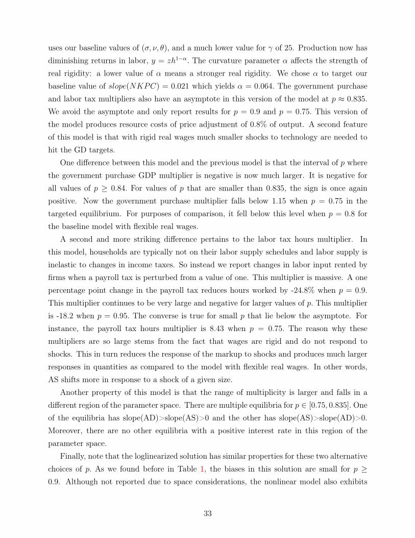
uses our baseline values of (σ, ν, θ), and a much lower value for γ of 25. Production now hasdiminishing returns in labor, y = zh1−α. The curvature parameter α affects the strength ofreal rigidity: a lower value of α means a stronger real rigidity. We chose α to target ourbaseline value of slope(NKPC) = 0.021 which yields α = 0.064. The government purchaseand labor tax multipliers also have an asymptote in this version of the model at p ≈ 0.835.

We avoid the asymptote and only report results for p = 0.9 and p = 0.75. This version ofthe model produces resource costs of price adjustment of 0.8% of output. A second featureof this model is that with rigid real wages much smaller shocks to technology are needed tohit the GD targets.

One difference between this model and the previous model is that the interval of p wherethe government purchase GDP multiplier is negative is now much larger. It is negative forall values of p ≥ 0.84. For values of p that are smaller than 0.835, the sign is once againpositive. Now the government purchase multiplier falls below 1.15 when p = 0.75 in thetargeted equilibrium. For purposes of comparison, it fell below this level when p = 0.8 forthe baseline model with flexible real wages.

A second and more striking difference pertains to the labor tax hours multiplier. Inthis model, households are typically not on their labor supply schedules and labor supply isinelastic to changes in income taxes. So instead we report changes in labor input rented byfirms when a payroll tax is perturbed from a value of one. This multiplier is massive. A onepercentage point change in the payroll tax reduces hours worked by -24.8% when p = 0.9.

This multiplier continues to be very large and negative for larger values of p. This multiplieris -18.2 when p = 0.95. The converse is true for small p that lie below the asymptote. Forinstance, the payroll tax hours multiplier is 8.43 when p = 0.75. The reason why thesemultipliers are so large stems from the fact that wages are rigid and do not respond toshocks. This in turn reduces the response of the markup to shocks and produces much largerresponses in quantities as compared to the model with flexible real wages. In other words,AS shifts more in response to a shock of a given size.

Another property of this model is that the range of multiplicity is larger and falls in adifferent region of the parameter space. There are multiple equilibria for p ∈ [0.75, 0.835]. Oneof the equilibria has slope(AD)>slope(AS)>0 and the other has slope(AS)>slope(AD)>0.Moreover, there are no other equilibria with a positive interest rate in this region of theparameter space.

Finally, note that the loglinearized solution has similar properties for these two alternativechoices of p. As we found before in Table 1, the biases in this solution are small for p ≥0.9. Although not reported due to space considerations, the nonlinear model also exhibits

33

a conventional configuration of demand and supply when p ≤ 0.3.28 In this interval, theloglinear solution exhibits a Type 1 equilibrium instead. The only difference is that the sizeof the bias in the labor tax multiplier is now larger for p in this range.

Overall, introducing real wage rigidities allows us to entertain smaller values of γ andthus smaller resource costs of price adjustment. Government purchase multipliers are stillsmall or negative for a broad range of values of p. The major shortcoming of the model withrigid wages is that the labor tax multipliers are now extraordinarily large. In addition, theregion with multiple zero bound equilibria is larger.

8 Conclusion

In this paper we have documented the global properties of the Rotemberg model at the zerobound and found that for a broad range of empirically relevant parameters the governmentpurchase multiplier is about one or less and there is no paradox of toil. Our results do not ruleout the possibility of large fiscal multipliers. As we have shown they can be arbitrarily largeand positive or arbitrarily large and negative when the slopes of the AD and AS schedulesare sufficiently close.

In the course of making these points, we have described the global properties of theRotemberg model of price adjustment. This model has a rich set of dynamics when interestrates are zero. At least four distinct configurations of AD and AS schedules occur includingthe conventional configuration with slope(AD)<0<slope(AS). In addition, there can be mul-tiple zero bound equilibria. These properties of the Rotemberg model arise in empiricallyrelevant ranges of the space of parameters and shocks.

Our analysis has focused on the properties of fiscal multipliers when the nominal rate ofinterest is zero. It is clear, though, that our findings are relevant for a broad range of otheranalyses of the zero bound. The properties of an optimal monetary policy are of particularinterest to us. The results on optimal monetary policy in e.g. Eggertsson and Woodford(2003) and Werning (2011) are derived in models that respect the nonlinearity in the Taylorrule but loglinearize the remaining equilibrium conditions about a steady state with a stableprice level. In our future work, we plan to consider the properties of monetary policy in anonlinear framework along the lines of the one we have considered here.

28A more complete set of results for this model is reported in the Online Appendix.

34

Appendix A Proofs

Proof of Proposition 1 The AD and the AS schedules are

πL = [slope(AD)zL − reLp

] + slope(AD)hL, and πL = slope(AS)σ − 1

σ + νzL + slope(AS)hL.

They are upward-sloping, for both slope(AD) and slope(AS) are positive.First, assume (1a) and (1b). They imply that the AD schedule is strictly steeper than

the AS schedule, and that the intercept term is strictly higher for the AD schedule than forthe AS schedule. It follows that at the intersection hL < 0. Solving for πL, we obtain

πL =1

slope(AS)− slope(AD)

[slope(AS){slope(AD)zL − reL

p} − slope(AD)slope(AS)

σ − 1

σ + νzL]

=slope(AS)

slope(AS)− slope(AD)

[slope(AD)zL + slope(AD)

σ − 1

σ + ν(−zL)− reL

p

].

Since slope(AS)− slope(AD) < 0, πL is negative at the intersection if and only if the termsin the square brackets are positive.

slope(AD)zL + slope(AD)σ − 1

σ + ν(−zL)− reL

p

≥ slope(AD)zL + slope(AS)σ − 1

σ + ν(−zL)− reL

p

(By assumption, (σ − 1)(−zL) ≥ 0 and slope(AS)− slope(AD) < 0.)

> 0. (By condition 1a).)

Thus, at the intersection of the AD and the AS schedules, (πL, hL) < (0, 0).What remains to show is that at the intersection, the Taylor rule implies zero nominal

interest rate. The linear part of the Taylor rule in (8) prescribes

re + φππL + φyy

L

< p

(slope(AD)− slope(AS)

σ − 1

σ + ν

)zL + φππ

L + φyyL. (Condition 1a).)

Since yL = zL + hL, we know that (zL, πL, yL) are all negative. Condition 1b) implies thatthe coefficient on zL is strictly positive. Together with the assumption (φπ, φy) ≥ 0, it followsthat the RHS of the above inequality is strictly negative, and the nominal interest rate atthe intersection is zero.

Next, assume (2a) and (2b). Proof is almost the same as that in the case with (1a) and

35

(1b). The only difference is that φπ needs to be sufficiently large to have reL+φππL+φyy

L < 0.Since the AD schedule is upward sloping and hL < 0, πL is smaller than the intercept of theAD schedule, slope(AD)zL − reL/p. Thus, the assumption φπ ≥ p implies

reL + φππL + φyy

L ≤ reL + pπL ≤ reL + p{slope(AD)zL − reL/p} ≤ p× slope(AD)zL ≤ 0.

The nominal interest rate is thus zero.Finally, suppose 1a) holds but 1b) doesn’t. Then the AD is no steeper than the AS, and

the intercept of the AD is larger than the intercept of the AS. When the AD and the AS areparallel but their intercepts differ, then there is no intersection and thus no equilibrium withR = 0. When the AS is strictly steeper than the AD, then their intersection satisfies hL > 0,and there is no ZLB equilibrium with hL ≤ 0. The same argument goes through for the casewhere 2a) holds but 2b) doesn’t.�

Proof of Proposition 2 We first solve for (hL, πL), allowing non-zero ηL and τLw . Definethe intercepts of the AS and AD schedules as

icept(AS) = −slope(AS)σ

σ + ν

1

1− ηηL + slope(AS)

1

σ + ν

1

1− τwτLw − slope(AS)

1− σσ + ν

zL

icept(AD) =−reLp− slope(AD)

1

1− ηηL + slope(AD)zL.

Then

hL =icept(AD)− icept(AS)

slope(AS)− slope(AD)

πL = icept(AS) + slope(AS)hL (= icept(AD) + slope(AD)hL)

Consider a paradox of toil: by differentiating (hL, πL) by τLw , we obtain

dhL

dτLw=

−slope(AS)

slope(AS)− slope(AD)

1

σ + ν

1

1− τw,

dπL

dτLw= slope(AD)

dhL

dτLw.

Under the Type 1 parameterization, both hours and inflation increase in response to anincrease in labor tax (dhL/dτLw and dπL/dτLw are positive), thereby establishing the paradox oftoil. Under the Type 2 parameterization, however, both dhL/dτLw and dπL/dτLw are negative,and both hours and inflation decline in response to an increase in labor tax.

Next, consider a change in government purchase share. Differentiating by ηL, we obtain

dhL

dηL=

1

1− ηslope(AS) σ

σ+ν− slope(AD)

slope(AS)− slope(AD),

dπL

dηL= slope(AD)[− 1

1− η+dhL

dηL].

36

Under the Type 1 parameterization, slope(AD) > slope(AS) > slope(AS)σ/(σ + ν) > 0,and thus dhL/dηL is positive and greater than 1/(1 − η). This further implies dπL/dηL ispositive. An increase in η thus increases both hours and inflation.

Under the Type 2 parameterization, it is either (1) slope(AD)− slope(AS)σ/(σ+ ν) > 0

or (2) slope(AD) − slope(AS)σ/(σ + ν) < 0. In the first case, both dhL/dηL and dπL/dηL

are negative. In the second case, we have 0 < dhL/dηL < 1/(1− η) and dπL/dηL < 0.We are more interested in the response of GDP to a change in government purchases than

a change in its share. Suppose for a moment that the government purchase g increases inresponse to an increase in η. In this case, the government purchase multiplier on GDP isgreater than one if and only if consumption increases in response to η. From the resourceconstraint c = (1 − η − κ)zh, we have dcL/dηL = −1/(1 − η) + dhL/dηL. We know fromthe preceding discussion that under the Type 1 (2) parameterization the right hand side ispositive (negative). Thus the government purchase multiplier is greater than one under theType 1 parameterization, and less than one under the Type 2 parameterization, as long asthe government purchases increase in response to an increase in η.

Finally, the government purchases decrease in response to an increase in η only whenhours respond negatively. This requires slope(AS) > slope(AD) > slope(AS)σ/(σ + ν).From g = ηzh, we have dgL/dηL = 1/η + dhL/dηL. This is less than zero if and only if

(1− η + ησ

σ + ν)slope(AS) < slope(AD).

Proof of Proposition 3: We loglinearize the AD relationship (13) around a referencepoint (hL, πL) which satisfies (13). Let ∆hL be the log deviation of hours and ∆πL be thelevel deviation of inflation rate from this reference point. This yields

∆hL ={ 1

σ

pβdL/(1 + πL)2

1− pβdL/(1 + πL)+

(κL)′

1− κL − ηL}

∆πL. (21)

This implies Proposition 3.

Proof of Proposition 4 We loglinearize the AS relationship around a reference point(hL, πL) which satisfies (14). Let (∆hL,∆πL) be the same as in the proof of Proposition 3.Then it yields

(σ + ν)∆hL ={ (1− pβdL)γ(1 + 2πL)

(1− pβdL)γπL(1 + πL) + θ+

σ(κL)′

1− κL − ηL}

∆πL. (22)

Since σ + ν > 0, Proposition 4 is implied.

37

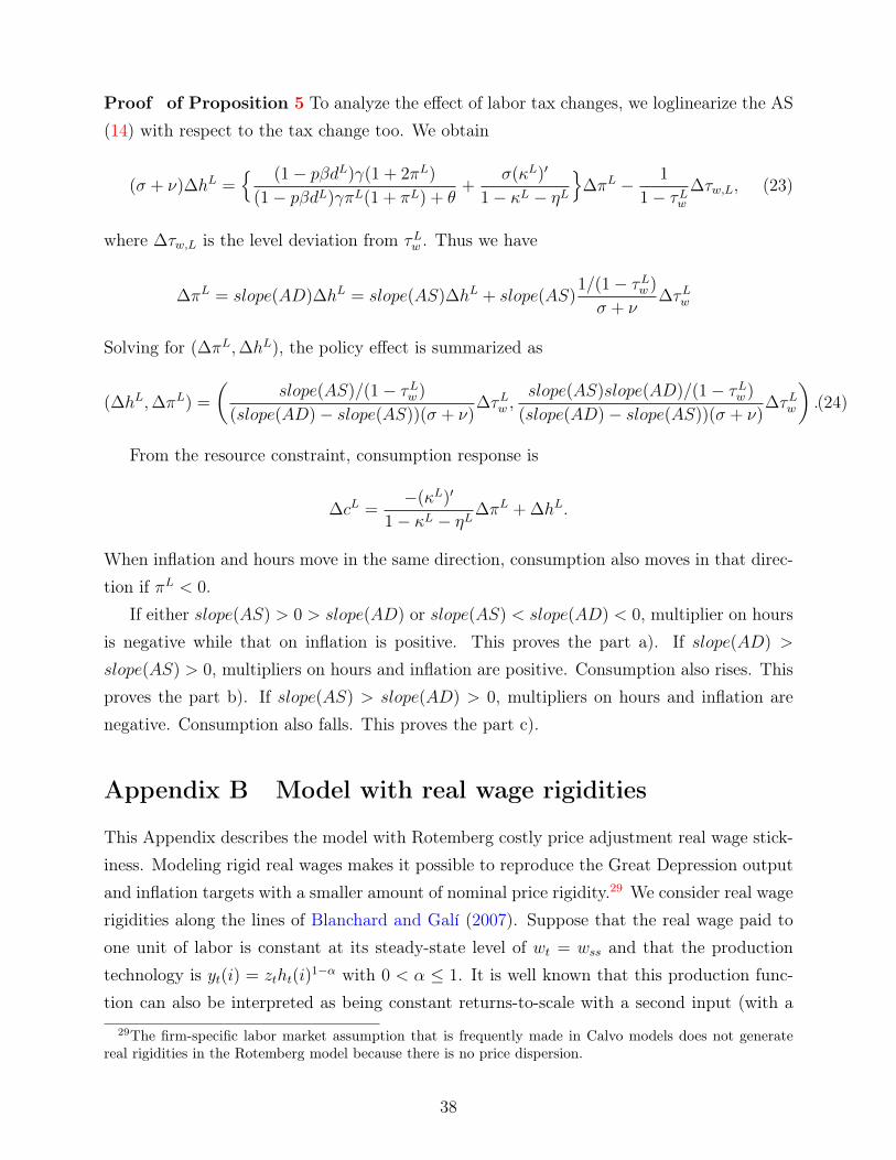
Proof of Proposition 5 To analyze the effect of labor tax changes, we loglinearize the AS(14) with respect to the tax change too. We obtain

(σ + ν)∆hL ={ (1− pβdL)γ(1 + 2πL)

(1− pβdL)γπL(1 + πL) + θ+

σ(κL)′

1− κL − ηL}

∆πL − 1

1− τLw∆τw,L, (23)

where ∆τw,L is the level deviation from τLw . Thus we have

∆πL = slope(AD)∆hL = slope(AS)∆hL + slope(AS)1/(1− τLw )

σ + ν∆τLw

Solving for (∆πL,∆hL), the policy effect is summarized as

(∆hL,∆πL) =

(slope(AS)/(1− τLw )

(slope(AD)− slope(AS))(σ + ν)∆τLw ,

slope(AS)slope(AD)/(1− τLw )

(slope(AD)− slope(AS))(σ + ν)∆τLw

).(24)

From the resource constraint, consumption response is

∆cL =−(κL)′

1− κL − ηL∆πL + ∆hL.

When inflation and hours move in the same direction, consumption also moves in that direc-tion if πL < 0.

If either slope(AS) > 0 > slope(AD) or slope(AS) < slope(AD) < 0, multiplier on hoursis negative while that on inflation is positive. This proves the part a). If slope(AD) >

slope(AS) > 0, multipliers on hours and inflation are positive. Consumption also rises. Thisproves the part b). If slope(AS) > slope(AD) > 0, multipliers on hours and inflation arenegative. Consumption also falls. This proves the part c).

Appendix B Model with real wage rigidities

This Appendix describes the model with Rotemberg costly price adjustment real wage stick-iness. Modeling rigid real wages makes it possible to reproduce the Great Depression outputand inflation targets with a smaller amount of nominal price rigidity.29 We consider real wagerigidities along the lines of Blanchard and Galí (2007). Suppose that the real wage paid toone unit of labor is constant at its steady-state level of wt = wss and that the productiontechnology is yt(i) = ztht(i)

1−α with 0 < α ≤ 1. It is well known that this production func-tion can also be interpreted as being constant returns-to-scale with a second input (with a

29The firm-specific labor market assumption that is frequently made in Calvo models does not generatereal rigidities in the Rotemberg model because there is no price dispersion.

38

fixed rental price) that cannot be adjusted in the very short-run. Following the example ofBlanchard-Gali we suppose that equilibrium labor is demand-determined and obeys

wt = (wt−1)γ(v′(ht)

u′(ct)(1− τw,t))1−γ

with γ = 1 and w−1 = wss. Firms are on their input demand schedules so this assumptionimplies that the after-tax real wage will not generally equal the household’s marginal rate ofsubstitution.

The cost function for firm i is now (1 + τP,t)wss/zt × yt(i)1

1−α , where τP,t is a payroll taxpaid by firms. Labor income tax cuts are neutral in this setting so we introduce a payrolltax to analyze the effect of changes in this tax wedge on labor. We set its steady state valueto zero.

Under our previous assumption that θ = (1 + τs)(θ − 1), the NKPC is given by:

γπt(1 + πt) =θ

1− α(1 + τP,t)

wsszthαt − θ + βdt+1Et[

u′(ct+1)

u′(ct)

yt+1

ytγπt+1(1 + πt+1)],

and the AS equation is given by

(1− pβdL)γ

θπL(1 + πL) =

wss(1− α)zL

(1 + τLP )(hL)α − 1.

Note that this is independent of the individual labor income tax rate τw, and thus an equi-librium is unaffected by changes in τw.

When loglinearized around (hL, πL) and τLP = τP ,

∆π =(1− pβdL)γ

θπL(1 + πL) + 1

(1− pβdL)γθ(1 + 2πL)

{α∆h+

∆τP

1 + τP−∆z

}.

The resource constraint isc = (1− κ− η)zh1−α.

and thus the loglinearized AD equation around (hL, πL) is

∆π =(1− pβdL

1+πL)σ

pβdL

(1+πL)2+ (1− pβdL

1+πL) σγπL

1−κL−ηL

{(1− α)∆h+ ∆z − ∆η

1− κL − ηL

}.

It follows that the tax multiplier on hours is given by

slope(AS)

slope(AD)− slope(AS)

1

α(1 + τP ).

39

References

Aruoba, S. B., and F. Schorfheide (2013): “Macroeconomic Dynamics Near the ZLB:A Tale of Two Equilibria,” NBER Working Papers 19248, National Bureau of EconomicResearch, Inc. 1, 3.1, 7, 6.1

Benhabib, J., S. Schmitt-Grohe, and M. Uribe (2001): “Monetary Policy and MultipleEquilibria,” American Economic Review, 91(1), 167–186. 1, 2.2, 3.1

Blanchard, O., and J. Galí (2007): “Real Wage Rigidities and the New KeynesianModel,” Journal of Money, Credit and Banking, 39(s1), 35–65. 7.3, B

Braun, R. A., L. Körber, and Y. Waki (2012): “Some unpleasant properties of log-linearized solutions when the nominal interest rate is zero,” Federal Reserve Bank of AtlantaWorking Paper 2012-5a. 3.1, 6

Braun, R. A., and Y. Waki (2010): “On the Size of the Fiscal Multiplier When the ZeroBound on Nominal Interest Rates is Binding,” mimeo. 1, 7.3

Broda, C., and D. Weinstein (2004): “Globalization and the gains from variety,” StaffReports 180, Federal Reserve Bank of New York. 5.1, 6.2.1

Bullard, J. (2010): “Seven Faces of “The Peril”,” Federal Reserve Bank of St. Louis Review,92(5), 339–352. 2.2, 3.1

Burgess, S., E. Fernandez-Corugedo, C. Groth, R. Harrison, F. Monti,

K. Theodoridis, and M. Waldron (2013): “The Bank of England’s Forecasting Plat-form: COMPASS, MAPS, EASE and the Suite of Models,” Bank of England working paper.5.1

Calvo, G. A. (1983): “Staggered prices in a utility-maximizing framework,” Journal ofMonetary Economics, 12(3), 383–398.

Carlstrom, C., T. Fuerst, and M. Paustian (2012): “Fiscal Multipliers under anInterest Rate Peg of Deterministic and Stochastic Duration,” mimeo. 1, 6.1

Christiano, L., and M. Eichenbaum (2012): “Notes on Linear Approximations, Equilib-rium Multiplicity and E-learnability in the Analysis of the Zero Bound,” mimeo. 1, 6.1,6.2.3, 17

40

Christiano, L., M. Eichenbaum, and S. Rebelo (2011): “When is the GovernmentSpending Multiplier Large?,” Journal of Political Economy, 119(1), 78–121. 1, 5.2, 17,6.2.3

Denes, M., G. B. Eggertsson, and S. Gilbukh (2013): “Deficits, Public Debt Dynamicsand Tax and Spending Multipliers,” Economic Journal, 0, 133–163. 5.1, 6.1, 6.2.4

Eggertsson, G. (2011): “What Fiscal Policy is Effective at Zero Interest Rates?,” in NBERMacroconomics Annual 2010, Volume 25, NBER Chapters, pp. 59–112. National Bureauof Economic Research, Inc. 1, 5.2, 6.2.3, 7.2

Eggertsson, G., A. Ferrero, and A. Raffo (2013): “Can Structural Reforms HelpEurope?,” Unpublished manuscript, Brown University. 1

Eggertsson, G., and P. Krugman (2012): “Debt, Deleveraging and the Liquidity Trap:A Fisher-Minsky-Koo Approach,” Quarterly Journal of Economics, 127(3). 1, 2.3

Eggertsson, G., and M. Woodford (2003): “The Zero Interest Rate Bound and OptimalMonetary Policy,” Brookings Panel on Economic Activity. 2, 2.2, 6.2.1, 8

Erceg, C., and J. Lindé (2010): “Is There a Fiscal Free Lunch in a Liquidity Trap?,” Boardof Governors Board of Governors International Finance Discussion Papers No. 1003. 1

Evans, G. W., E. Guse, and S. Honkapohja (2008): “Liquidity traps, learning andstagnation,” European Economic Review, 52(8), 1438–1463. 1

Fernandez-Villaverde, J., G. Gordon, P. A. Guerron-Quintana, and J. Rubio-

Ramirez (2012): “Nonlinear Adventures At The Zero Lower Bound,” NBER WorkingPaper 18058. 1

Gust, C., D. Lopez-Salido, and M. E. Smith (2012): “The empirical implications ofthe interest-rate lower bound,” Finance and Economics Discussion Series 2012-83, Boardof Governors of the Federal Reserve System (U.S.). 1, 5.1

Hayashi, F., and J. Koeda (2013): “A Regime-Switching SVAR Analysis of QuantitativeEasing,” CARF F-Series CARF-F-322, Center for Advanced Research in Finance, Facultyof Economics, The University of Tokyo. 12

Ireland, P. N. (2003): “Endogenous money or sticky prices?,” Journal of Monetary Eco-nomics, 50(8), 1623–1648. 5.1

41

Levy, D., M. Bergen, S. Dutta, and R. Venable (1997): “The Magnitude of MenuCosts: Direct Evidence from Large U. S. Supermarket Chains,” The Quarterly Journal ofEconomics, 112(3), 791–824. 6.1

Mertens, K., and M. O. Ravn (2010): “Fiscal Policy in an Expectations Driven LiquidityTrap,” CEPR Discussion Papers 7931, C.E.P.R. Discussion Papers. 1, 3.1, 6.1

Rotemberg, J., and M. Woodford (1997): “An Optimization-Based Econometric Frame-work for the Evaluation of Monetary Policy,” in NBER Macroeconomics Annual 1997,Volume 12, NBER Chapters, pp. 297–361. National Bureau of Economic Research, Inc.5.1

Rotemberg, J. J. (1982): “Sticky Prices in the United States,” Journal of Political Econ-omy, 90(6), 1187–1211. 1, 2

Werning, I. (2011): “Managing a Liquidity Trap: Monetary and Fiscal Policy,” mimeo. 8

Woodford, M. (2011): “Simple Analytics of the Government Expenditure Multiplier,”American Economic Journal: Macroeconomics, 3(1), 1–35. 1, 6.1

Yun, T. (2005): “Optimal Monetary Policy with Relative Price Distortions,” AmericanEconomic Review, 95(1), 89–109. 2.1

42

Table 1: Zero Bound Equilibrium Great Recession: (γ = 458.4, ν = 0.28)

Specification dL p zL κL × 100 Slope(AD) Slope(AS) ∆GDP∆G

∆h∆τw

Parameterization 1) 1.008 0.90 0.94Exact solution 1 0.14 0.12 0.29 0.62 -1.66Loglinear solution 0.22 0.11 0.21 0.62 -2.09

Parameterization 2) 1.01 0.86 0.95Exact solution 1 0.14 0.193 0.192 5.49 163.2Exact solution 2* 0.09 0.182 0.183 6.52 -172.7Loglinear solution 0.11 0.16 0.15 2.49 11.5

Parameterization 3) 1.015 0.80 0.95Exact solution 0.14 0.35 0.13 1.14 0.55Loglinear solution 0.14 0.25 0.11 1.18 0.72

Parameterization 4) 1.029 0.60 0.98Exact solution 0.14 5.65 0.056 1.02 0.010Loglinear solution 0.14 0.67 0.053 1.04 0.085

Parameterization 5) 1.037 0.50 0.99Exact solution 0.14 -2.76 0.043 1.008 -0.015loglinear solution 0.15 1.000 0.043 1.02 0.044

The size of the demand and technology shocks are chosen so that the exact solution produces a 7% decline in GDP and a 1% annualizeddecline in the inflation rate. The values of κL for the loglinearized solution are imputed.*This solution does not reproduce the targets.

43

Table 2: Zero Bound Equilibrium Great Recession: Our estimates (γ = 458.4, ν = 0.28) demand shock only.

Specification dL p θ κL × 100 Slope(AD) Slope(AS) ∆GDP∆G

∆h∆τw

Parameterization 1) 1.0076 0.90 1.28Exact solution 0.14 0.12 0.036 1.085 0.41Loglinear solution 0.12 0.11 0.035 1.079 0.45

Parameterization 2) 1.015 0.80 2.55Exact solution 0.14 0.35 0.036 1.030 0.11Loglinear solution 0.13 0.25 0.035 1.029 0.16

Parameterization 3) 1.029 0.60 5.15Exact solution 0.14 5.65 0.036 1.010 0.006Loglinear solution 0.14 0.67 0.036 1.010 0.055

Parameterization 4) 1.037 0.50 6.47Exact solution 0.14 -2.76 0.036 1.007 -0.013Loglinear solution 0.15 1.000 0.036 1.007 0.037

The size of the demand shock and the value of θ are chosen so that the exact solution reproduces a targeted decline in output of 7% andannualized inflation decline of 1%. The values of κL for the loglinearized solution are imputed.

44

Table 3: Zero Bound Equilibria Great Recession

Parameterization dL p γ θ κL × 100 Slope(AD) Slope(AS) ∆GDP∆G

∆h∆G

∆h∆τw

1) Christiano and Eichenbaum (CE) (2012) 1.012 0.775 100 3Exact solution (ES) 0.7 0.46 0.31 2.18 1.71 1.32Loglinear solution (LLS) 1.6 0.29 0.26 2.77 2.77 4.95

2) CE (2012) calibrated using ES, 1.0237 0.775 300 1.24Exact solution 0.09 0.36 0.034 1.06 1.04 0.066Loglinear solution 0.09 0.29 0.035 1.05 1.05 0.087

3) Denes et al. (2013) calibrated using ES, 1.0135 0.857 6345 13.23Exact solution 2.0 -0.067 0.057 1.08 0.792 -0.20Loglinear solution 3.0 0.204 0.0416 1.12 1.12 0.11

4) Denes et al. (2013) low γ calibrated using ES, 1.0266 0.70 720 13.23Exact solution 0.23 -5.89 0.11 1.04 1.05 -0.016Loglinear solution 0.19 0.52 0.091 1.09 1.09 0.18

Results labeled “calibrated” have been calibrated to produce a 7% GDP decline and 1% annualized inflation decline using the specified solution.The values of κL for the loglinearized solution are imputed.

45

Table 4: Zero Bound Equilibria Great Depression

Specification dL p zL γ θ κL Slope(AD) Slope(AS) ∆GDP∆G

∆h∆G

∆h∆τw

1) Our estimates calibrated using ES,Parameterization a) 1.042 0.80 0.93 458.4 7.67Exact solution (ES) 0.155 -0.080 -0.23 1.13 0.91 -1.50Loglinear solution (LLS) 0.121 0.25 0.11 1.20 0.72

Parameterization b) 1.059 0.75 1.00 458.4 7.67Exact solution 0.155 -0.071 -0.99 1.061 0.96 -1.05Loglinear solution 0.145 0.33 0.085 1.064 0.33

Parameterization c) 1.063 0.74 1.009 458.4 7.67Exact solution 0.155 -0.070 -3.92 1.054 0.96 -0.99Loglinear solution 0.149 0.35 0.082 1.043 0.30

Parameterization d) 1.067 0.73 1.023 458.4 7.67Exact solution 0.155 -0.069 1.87 1.047 0.96 -0.94Loglinear solution 0.153 0.37 0.079 1.023 0.26

Parameterization e) 1.078 0.70 1.070 458.4 7.67Exact solution 0.155 -0.067 0.32 1.034 0.95 -0.81Loglinear solution 0.166 0.43 0.071 0.97 0.19

2) Eggertsson (2011), calibrated using LLS, 1.0134 0.903 1 4059.78 12.77Exact solution 0.11 -0.033 -0.22 1.20 0.43 -0.54Loglinear solution 1.24 0.12 0.086 1.82 1.02

3) Eggertsson (2011), calibrated using ES, 1.0213 0.903 1 1209.2 12.77Exact solution 1 0.41 -0.015 -0.032 1.26 -0.24 -0.87Exact solution 2* 0.11 0.031 0.077 0.76 0.068 -0.76Loglinear solution N.A. N.A. N.A. N.A. N.A. N.A.

4) Rigid wage model, calibrated using ES, 1.0051 0.9 0.989 25 7.67Exact solution 0.0084 0.078 0.21 -1.00 -0.928 -24.83Loglinear solution 0.017 0.10 0.19 -2.22 -28.45

5) Rigid wage model, calibrated using ES, 1.0505 0.75 0.998 25 7.67Exact solution 0.0084 0.271 0.095 1.48 1.47 8.43Loglinear solution 0.039 0.312 0.078 1.31 4.33

For results labeled “calibrated” model is calibrated to produce a 30% GDP decline and a 10% inflation decline using the specified solution.The values of κL for the loglinearized solution are imputed.* This solution does not hit the targets.

46

Figure 1: Government purchase multipliers and labor tax hours multipliers.

0.2 0.4 0.6 0.8

0

0.2

0.4

0.6

0.8

1

p

Tax multiplier on hours: 0.05 ) p ) 0.8

0.8 0.82 0.84

2

4

6

8

10

p

Tax multiplier on hours: 0.8 ) p ) 0.86

0.88 0.9 0.92 0.94ï15

ï10

ï5

0

p

Tax multiplier on hours: 0.865 ) p ) 0.95

0.2 0.4 0.6 0.80.95

1

1.05

1.1

1.15

p

g multiplier on GDP: 0.05 ) p ) 0.8

0.8 0.82 0.841

1.5

2

2.5

3

p

g multiplier on GDP: 0.8 ) p ) 0.86

0.88 0.9 0.92 0.94ï6

ï4

ï2

0

2

4

p

g multiplier on GDP: 0.865 ) p ) 0.95

0.2 0.4 0.6 0.80.95

1

1.05

1.1

1.15

p

g multiplier on hours: 0.05 ) p ) 0.8

0.8 0.82 0.841

1.5

2

2.5

3

p

g multiplier on hours: 0.8 ) p ) 0.86

0.88 0.9 0.92 0.94ï6

ï4

ï2

0

2

4

p

g multiplier on hours: 0.865 ) p ) 0.95

LLNL (target)

LLNL (target)

LLNL (target)NL (nonïtarget)

LLNL (target)

LLNL (target)

LLNL (target)NL (nonïtarget)

LLNL (target)

LLNL (target)

LLNL (target)NL (nonïtarget)

NL refers to the multipliers using the exact solution and LL refers to multipliers using the loglin-earized solution. Scaling: A value of one implies that a one percentage point change in the labortax results in a one percent increase in hours.

47

Figure 2: Government purchase GDP multipliers and labor tax hours multipliers in a modelwith no technology shock.

0.1 0.2 0.3 0.4 0.5 0.6 0.7 0.8 0.9ï0.1

0

0.1

0.2

0.3

0.4

p

Tax multiplier on hours: 0.05 ) p ) 0.9

LLNL (target)

0.9 0.91 0.92 0.93 0.940

0.5

1

1.5

2

p

Tax multiplier on hours: 0.9 ) p ) 0.95

LLNL (target)

0.1 0.2 0.3 0.4 0.5 0.6 0.7 0.8 0.90.95

1

1.05

1.1

p

g multiplier on hours: 0.05 ) p ) 0.9

LLNL (target)

0.9 0.91 0.92 0.93 0.941

1.1

1.2

1.3

1.4

p

g multiplier on hours: 0.9 ) p ) 0.95

LLNL (target)

0.1 0.2 0.3 0.4 0.5 0.6 0.7 0.8 0.90.95

1

1.05

1.1

p

g multiplier on GDP: 0.05 ) p ) 0.9

LLNL (target)

0.9 0.91 0.92 0.93 0.941

1.1

1.2

1.3

1.4

p

g multiplier on GDP: 0.9 ) p ) 0.95

LLNL (target)

NL refers to the multipliers using the exact solution and LL refers to multipliers using the loglin-earized solution. Scaling: A value of one implies that a one percentage point change in the labortax results in a one percent increase in hours.

48