sound reproduction by wave field synthesis · vi contents 2.2.1 rayleigh i integral 34 2.2.2...
TRANSCRIPT

Sound
Reproduction
by
Wave Field Synthesis
Edwin Verheijen

Sound Reproduction
by
Wave Field Synthesis
Edwin Verheijen

Copyright © 1997 (first edition) and 2010 (second edition) by Edwin Verheijen
The first edition of this thesis was published in hard copy only. In 1997, a document formatlike PDF was hardly known. This second edition is only available as PDF, to provide full textsearch capabilities to the reader.
The original text is unchanged, except for two or three typing errors. As none of the orig-inal computed graphs have been preserved, I have included these as scans, taken from the hardcopy. Unfortunately, Chapter 1 and two appendices were destroyed completely (on 3.5 inchdiskette). For this reissue, I took the trouble to edit a recovered ASCII text version of Chapter1 into a new Chapter 1. Besides the graphs, also the equations in this chapter will appear asscanned pictures. The appendices were not preserved in any form, except hard copy. These areincluded as scans, and will remain non-searchable.
SUPPORTThis work has been supported by the Dutch Technology Foundation (STW) and Philips Re-search Laboratories, The Netherlands.
Language: English, with additional summaries in German, French and Dutch.
Utrecht, 28th May 2010

De sorte qu’il faut qu’autour de chaque particule il se fasse une onde dont cette particule soit le centre.
Christiaan Huygens (1629-1695)Traité de la Lumière, Leyden, Holland, 1690.

v
Contents
Chapter 1 Introduction 1
1.1 A century of sound reproduction 1 1.2 Objectives 2 1.3 Room acoustics 3 1.4 S patial perception 6 1.5 Sound reproduction requirements 9 1.6 Two-channel stereophony 10
1.6.1 Loudspeaker set-up 10 1.6.2 Reproduction techniques 11 1.6.3 Microphone and mixing techniques 18 1.6.4 Spectral properties of stereophony 22 1.6.5 Binaural recording and reproduction 22
1.7 Surround sound systems 23 1.7.1 Quadraphony 23 1.7.2 Dolby Surround 24 1.7.3 Ambisonics 25 1.7.4 Surround sound in the cinema 27 1.7.5 Discrete surround sound at home 28
1.8 Conclusions 29
Chapter 2 Wave Field Synthesis 31
2.1 lntroduction 31 2.2 Kirchhoff-He1mholtz Integral 32

vi Contents
2.2.1 Rayleigh I integral 34 2.2.2 Rayleigh II integral 36
2.3 Synthesis operator for line distributions 36 2.3.1 2½ D Synthesis operator 37 2.3.2 Focusing operator 45 2.3.3 Generalization of 2½D -operators 48
2.4 Diffraction waves 50 2.4.1 Truncation effects 50 2.4.2 Corner effects 53
2.5 Discretization 54 2.5.1 Plane wave decomposition 56 2.5.2 Spatial sampling and reconstruction 58
2.6 Applications of wave field synthesis 62 2.7 Conclusions 62
Chapter 3 Loudspeaker Arrays 63
3.1 Introduction 63 3.2 Loudspeaker types 64
3.2.1 Canonical equations 64 3.2.2 Electrodynamic loudspeaker 64 3.2.3 Electrostatic loudspeaker 67
3.3 Directivity 69 3.3.1 Spatial Fourier transform and directivity 70 3.3.2 Spatial low-pass filter by diaphragm shaping 73 3.3.3 Spatial low-pass filter by discrete spatial convolution 75
3.4 Design of arrays for audio reproduction 78 3.4.1 Electrodynamic array 79 3.4.2 Electrostatic array 83 3.4.3 Comparative measurements 85
3.5 Conclusions 88
Chapter 4 Concept and Implementation of WFS Reproduction 89
4.1 Introduction 89 4.2 General concept 90
4.2.1 ldeal solutions for reproduction 90 4.2.2 Practical solutions for reproduction 91 4.2.3 Recording 93 4.2.4 Transmission 97 4.2.5 Playback 97 4.2.6 Compatibility 99
4.3 Laboratory demonstration system 101 4.3.1 Overview 101

vii Contents
v
4.3.2 Array configuration 102 4.3.3 DSP-system hardware 104 4.3.4 DSP-system software 104
4.4 Applications of the new concept 110 4.4.1 Living-room 110 4.4.2 Cinema 111 4.4.3 Virtual reality theater 111 4.4.4 Simulators 111 4.4.5 Acoustic research 111
4.5 Conclusions 112
Chapter 5 Objective Evaluation 113
5.1 Introduction 113 5.2 System response 113
5.2.1 Frequency response 114 5.2.2 Spatial response 114 5.2.3 Focal pressure-distribution 116
5.3 Comparison between reproduction systems 118 5.3.1 Introduction 118 5.3.2 Dummy-head measurements 120 5.3.3 Multi-trace impulse responses 125 5.3.4 Intensity measurements 126 5.3.5 Frequency spectrum measurements 133
5.4 Conclusions 134
Chapter 6 Subjective Evaluation 137
6.1 Introduction 137 6.2 Localization experiments 137
6.2.1 Virtual sources behind the array (exp. A) 139 6.2.2 Virtual sources in front ofthe array (exp. B) 144 6.2.3 Evaluation of both experiments 145 6.2.4 Distance perception 147
6.3 Comparison between reproduction systems 148 6.3.1 Introduction 148 6.3.2 Experimental set-up 149 6.3.3 Evaluation 150
6.4 Conclusions 152

viii Contents
Appendix A Derivation of the 2½D Focusing Operator 153
Appendix B Recording and Mixing of Musical Performances for Subjective Evaluation 157
Author Index 161
Subject Index 163
References 167
Summary 173
Zusammenfassung 175
Sommaire 177
Samenvatting 179
1
Chapter 1
Introduction
1.1 A century of sound reproduction
The history of sound reproduction starts with the invention of the phonograph by Thomas Alva Edison in 1877. The apparatus consisted of a diaphragm with a stylus that transferred sound waves into indentations in a piece of tinfoil wrapped around a rotating cylinder. In order to reproduce the `stored' sound, the cutting stylus had to be replaced by a playback stylus, slid-ing through the grooves with less pressure (Butterworth 1977). Edison presented his apparatus as a human voice recorder.
The acousto-mechanical phonograph integrated three essential components for sound reproduction: the recording transducer, the recording medium and the playback transducer. Through the application of electricity it was no longer necessary to keep the essential parts together in one single machine. In the 1920s the condenser microphone (Massa 1985) and the electrodynamic loudspeaker (Hunt 1982) were successfully introduced. These transducers would basically remain unaltered until the present, unlike the recording medium. Flat record discs were already common practice, but still had to compete with cylindrical records. Other media like metal particle tape and magnetic disc (`hard disc') were also considered, but proved premature (Camras 1985).
Until 1930, sound was reproduced in mono. The success of motion pictures in the 1930s ushered in an era of multi-channel sound. Great pioneering work was done by Blumlein (1931), who patented a system of sound pickup and reproduction that we would now call intensity stereophony. Steinberg and Snow (1934) used three spaced microphones to record sound, intended for playback through loudspeakers placed left, center and right. The work of De Boer

2 Chapter 1: Introduction
(1940) was of great importance for the understanding of stereophonic imaging. Multi-track recordings on magnetic tape became possible just after World War II, but the public had to wait until 1958 before two-channel stereophonic records became commercially available. The 16-inch long-playing vinyl disc, played at 33.3 rpm, would grow extremely popular in the next quarter of a century.
In the early 1970s, an attempt was made to extend the number of reproduction channels. A variety of multi-channel systems was proposed, collectively known as quadraphony (see e.g. Eargle 1971 and Cooper et al. 1972). Two additional loudspeakers were placed to the back or sides of the listener. The demand of compatibility forced researchers to develop so-called matrix systems, with four reproduction channels encoded in two transmission channels. Due to lack of standardization and moderate sound quality, quadraphony failed to conquer the con-sumer market.
The concept of matrix systems, however, was not abandoned by motion picture industry. Cinema already had a long tradition in multi-channel sound, and Dolby Stereo became a stan-dard encoding matrix in the 1980s. Two-channel `surround sound' recordings on videotape (for use at home) could be decoded to four channels: left, center, right and rear. Surround sound entered the living-room.
Meanwhile, a great improvement in sound reproduction quality was offered by Compact Disc, introduced in 1982. This optical medium provides two-channel recordings with enlarged recording duration, bandwidth and dynamic range of the (digitally stored) audio signals. It is expected that digital techniques will give a new impulse to multi-channel audio and video sys-tems in the near future.
1.2 Objectives
In this thesis a new method of sound reproduction is presented. This method is close to the physics of sound fields, because it attempts to re-create the original sound field. Therefore the original sound field is decomposed in its elementary temporal and spatial properties, trans-mitted, and finally synthesized to produce the original sound field again. This approach, based on wave field synthesis (Berkhout 1988 and Berkhout et al. 1993), offers a large listening area with equal and high reproduction quality for all listeners. Besides that, the sound engineer is given a powerful tool to re-arrange sources without degrading the sound image. Acoustic cor-rections to the original sound image can easily be applied, and if desired, the original acoustic impression can be replaced by the ambience of a different room.
This chapter will give a survey of room acoustics and psycho-acoustics. Afterwards the concepts of stereophonic reproduction systems will be discussed. Chapter 2 is a treatise on wave field synthesis. The driving functions for the synthesizing loudspeaker arrays will be derived from the starting point of the Kirchhoff-Helmholtz integral. Two types of loudspeaker arrays will be discussed in Chapter 3. In Chapter 4 the design of the complete reproduction system is described. Finally, Chapters 5 and 6 attempt to give an objective and subjective qual-ification of the reproduction system in comparison to other systems.

3
1.3 Room acoustics
Sound is a propagating pressure fluctuation in a fluid. If the medium is homogeneous, sound will extend radially, thus creating spherical waves (Figure 1.1). The magnitude of the pressure fluctuations is inversely dependent on the distance to the source of the sound. For an omnidirectional or monopole source, the sound pressure p can be written as:
(1.1)
where r is the distance from the source, t is the time, c is the propagation velocity (340 m/s in air at 1 atm., 20º C), and s(t) is the source signal. This equation states that the source signal remains unaltered during propagation, except for its amplitude.
Figure 1.1 Snapshot of the sound pressure of a monochromatic sound source in free space. The magnitudes are displayed as grayscale levels. Cross-section a-b shows the momentary magnitude of the pressure. The decrease of the envelope is inversely proportional to the distance of the source.

4 Chapter 1: Introduction
A well-known measure related to sound pressure is the decibel (dB). The dB-scale is a relative scale: the root mean square of the sound pressure is compared with a reference pressure. The sound pressure level (SPL) is given by
(1.2)
with p0 = 20 µPa, the pressure of a just noticeable 1 kHz tone for people with normal hearing. If sound is produced inside a room, the wave fronts will reach the walls within a few
milliseconds. Most of the sound energy is bounced back into the room; only part of the energy is absorbed by the walls. The reflected sound wave will be bounced repeatedly by successive walls until it has vanished by absorption. In a small room, e.g. a living-room, one is hardly aware of these reflected waves during a conversation. A hand-clap, however, provides enough peaked energy to let the reflections decay audibly. The effect is much stronger in a large room such as a concert-hall or a church, while it is absent in free field. In acoustics, listening to a hand-clap has evolved to measuring an impulse response. Impulsive sounds, such as produced by alarm pistols, have been replaced by much more controllable measurement signals like sweep-tones (Berkhout et al. 1980) and bursts of maximum length sequences (Rife 1989).
The impulse response is widely regarded as the most meaningful characteristic in room acoustics. Many acoustic parameters related to concert-hall acoustics, such as the reverberation time T60, can be derived from it. For measurements of impulse responses, an omnidirectional sound source (a loudspeaker system producing spherically symmetric sound waves) is placed at a position of interest, e.g. on stage where musical instruments are found during concerts. The measurement signal, fed to the sound source, is received by a microphone in the audience area and processed afterwards to give a unique impulse response for that source-receiver combination.
Figure 1.2 shows an impulse response measured in a shoebox-shaped concert-hall. Within a few milliseconds after the direct sound the reflections arrive. The reverberation tail is said to begin where the reflection density is so high that no individual reflections can be discriminated anymore, which is usually after 80 to 120 ms. An important property of reverberation is that its sound pressure level for steady state signals is more or less independent of the source-receiver distance. If the steady state source signal is switched off, the reverberation level will decrease approximately linear in time due to absorption (i.e. the reverberation tail in an impulse response decays exponentially). The reverberation time T60 is defined as the time it takes before the sound pressure level has dropped by 60 dB. Typical values for T60 are about 1 second for lecture halls, 2 seconds for concert-halls and 5 seconds for cathedrals. Concert-hall acoustics is reviewed recently by Beranek (1996).

5
Figure 1.2 Impulse response of the Stadsgehoorzaal in Leyden, the Netherlands. The time-axis is aligned with the arrival of direct sound. Source and receiver are 13 m apart. Some strong early reflections can still be distinguished, but later reflections tend to vanish in reverberation.
Consider a trumpet being played on stage while a microphone has been placed in the
audience area. Disregarding the directivity pattern of the trumpet, it is possible to calculate the pressure at the microphone p(t), if the impulse response h(t) for the corresponding source-receiver combination is known:
, (1.3a)
or, by introduction of the convolution symbol (asterisk),
. (1.3b)
where str(t) is the trumpet's output signal as would be recorded by a microphone close to the horn. Note that for causal impulse responses the lower time boundary (–∞) of the integral is replaced by 0. It may be more appropriate to rewrite this equation in the frequency domain. After substitution of the inverse Fourier transform of h(t), given by
, (1.4)
and a similar expression for str(t) into integral (1.3a) we can evaluate the Fourier transform
(1.5)
to

6 Chapter 1: Introduction
, (1.6)
according to the rule `convolution in the time-domain equals multiplication in the frequency-domain'. In terms of signal processing it can be said that the trumpet's spectrum is filtered by the transfer function of the concert-hall. Any other system with the same transfer function can replace the influence of the concert-hall on the sound of the trumpet. But there is more to a concert-hall than only this one-dimensional transfer function. Most of the spatial information of the sound field is missed in the signal p(t). Listening to the signal p(t) would give a faint idea about the spatial environment, but it would fail to provide a spatial sound image*. Spatial perception of sound is the subject of the next paragraph.
1.4 Spatial perception
Some basic knowledge on the perception of sound is necessary to understand the requirements for a sound reproduction system. The human auditory system is able to retrieve a spatial sound image of an acoustic event. Table 1.1 gives a few examples of such sound images that would occur to a listener by careful listening (while disregarding information of other senses).
Table 1.1 Examples of sound images
acoustic event temporala information spatial information
classic concert the melody of a cello;
the timbre of the tenor
concert hall; the cello is to the right;
the singer is in front of the orchestra
jazz concert rhythm of a snare drum;
words of a singer
a small jazz-club; the stage is to the left
the snare drum echoes from the backwall
street scene
(film)
klaxon of a car;
scream of a cat
narrow street; the car is nearby;
the cat is far-away
nature scene
(documentary)
shouting of a shepherd;
rumbling of a herd
vast moor (`dry' sound);
the shepherd is behind the herd a.Though spectral and temporal aspects of sound are quite distinct from a perceptual point of view, they are
physically equivalent via Fourier theory.
By introspection of a sound image, the auditory system can distinguish to a certain extent
between temporal information and spatial information. Temporal information is mainly related to the sound source, but can also be influenced by spatial conditions. Spatial information depends primarly on the geometry of the room, but is at its turn dependent on the kind of
* A spatial sound image is possible if the impulse responses are measured at both ears of a (dummy) head instead
of with one free standing microphone, see Section 1.6.5.

7
source signal. A clear distinction between temporal and spatial perception is therefore not possible.
Three important phenomena of spatial hearing are discussed briefly here: localization, spaciousness and perception of reverberation. Finally, a remark is made on the interaction between the auditory and the visual system.
Localization
The localization of sound sources is due to a combination of directional and distance hearing (Blauert 1983). In anechoic circumstances, the localization blur* of sources in the horizontal plane is in the order of 1º (straight ahead). To the sides this is higher: 10º (Figure 1.3). In the median plane also a value in the order of 10º is found. Directional localization of impulsive sounds in the horizontal plane is independent of the room reverberation time (Hartmann 1983). It is therefore believed that the first arriving wave front (direct sound) establishes the direction of the auditory event.
The human auditory system uses interaural time differences (ITD) and interaural level differences (ILD) for localization in the horizontal plane. Sound arriving at the head from left will reach the left eardrum earlier than the right eardrum. For frequencies below 1500 Hz the ITD is the main cue, while for higher frequencies the ILD plays an important role, next to the ITD of the envelope of the ear signals. Directional hearing in the median plane is based on head and torso cues, i.e. on spectral effects of diffraction from head and torso. In case of con-
Figure 1.3 Accuracy of auditory directional localization.
* Localization blur is the smallest change of source position that can just be noticed by a subject.

8 Chapter 1: Introduction
flicting ITD's, ILD's and head and torso cues, the ITD cue is dominant as long as low frequencies are incorporated (Wightman et al. 1992).
For distance hearing in anechoic circumstances a reference sound is needed: if the listener is unfamiliar with the sound, the estimated distance depends only on the loudness, not on the real distance. This implies that the curvature of the wave front is not a cue for distance hearing, at least not for far-away (>1 m) sources. For nearby sources (<1 m), frequency-dependent diffraction of the waves around the head provides distance cues. In reverberant spaces, the main cue for distance determination is the level difference between direct sound and reverberation. Such a judgement is based on the fact that the reverberation level is more or less independent of distance, while the direct sound follows the 1/r-law.
Spaciousness
In the foregoing, attention was paid to direct sound and reverberation. For a relatively long time the perceptual effects of reflections were scarcely understood. Since the late 1960s the notion has grown that reflections are responsible for a sense of spaciousness as found in good concert-halls. Barron (1971) recognized the importance of early lateral (from the sides) reflections, since they contribute to a `spatial impression'. Potter (1993) refers to this impression as `subjective broadening of the sound source'. He found that frequencies above 1500 Hz do not contribute significantly to spaciousness. Bradley et al. (1995) suggested that there may be two distinct notions of spaciousness: `apparent source width' and `listener envelopment', each connected to different temporal parts of the impulse response. In their opinion the apparent broadening of the source is related to the early lateral reflections, arriving no later than 80 ms after the direct sound. A sense of envelopment is felt due to later arriving lateral reflections.
Perception of reverberation
A gradual transition from late arriving reflections to reverberation is made after about 100 to 120 ms, where the fine structure of the reflections has more or less a stochastic nature. Reverberation is perceived as a gentle slurring of the sound. Reverberation is appreciated if no particular direction of incidence can be associated with it: if the direct sound stops abruptly, a diffuse and smoothly decaying sound is left.
Vision
The perception of a sound image may be influenced strongly by other sensations, especially those of the visual system. E.g. if visual cues are presented to the listener as well, these will dominate in localization. This phenomenon is known as the ventriloquist illusion. It states that sound will be localized at the apparent visual source if the discrepancies between visual and auditory cues are within certain boundaries.
It is the aim of this research to develop a reproduction system that can be used either with or without accompanying vision (e.g. film or television). The requirements for a reproduction

9
system must therefore be attuned to the more demanding case of sound reproduction in absence of vision.
1.5 Sound reproduction requirements
For many reasons it may be desired to record and reproduce the acoustic properties of a sonic event. For instance, a musical performance can only be attended by a limited number of people. By recording the event, and afterwards selling or broadcasting the recording, many more people are given the opportunity to have a notion of the original performance. If the suggestion of the reproduced event is so strong that a listener can hardly distinguish it from a real event, acoustic virtual reality becomes feasible. In this paragraph, requirements for realistic sound reproduction are discussed.
Since it is thought that the purpose of a reproduction system is to evoke the same sound
image as would be done by the original sound field, an exact copy of the original sound field would be the simplest criterion. However, seen in the light of the perceptual limitations of the auditory system, a less demanding set of criteria will suffice. Such criteria must be based on psycho-acoustic knowledge. The question is therefore: which attributes of the (original) sound image are relevant? The answer can be divided in temporal and spatial attributes. In general, temporal requirements will be fulfilled if highly linear reproduction equipment with sufficient bandwidth and dynamic range is used. The spatial requirements follow the attributes of spatial hearing:
1. Correct localization. Direction and distance of reproduced sources should approach the position of the original sources as close as possible.
2. Correct spaciousness. The spatial impression of the original acoustic environment should be preserved.
3. Correct degree of diffuseness of the reverberant field. The reproduced reverberation must sound equally diffuse as the reverberation in the original environment.
The most important demand is however that the above requirements should be satisfied in a large listening area, large enough to accommodate several listeners. It is the motivation for the present research to come to a reproduction method that offers equal conditions for sound imaging in a large reproduction room. It is found that conventional reproduction methods have severe shortcomings at this point. An understanding of the underlying theory of present day reproduction systems is necessary to identify the causes of these problems. In the following paragraphs a review of current reproduction methods is given.

10 Chapter 1: Introduction
1.6 Two-channel stereophony
Two reproduction channels are a minimal condition for spatial sound reproduction. Two-channel reproduction basically falls apart in two groups of techniques, distinct by their objectives.
1. True stereophony aims at the reproduction of a natural sound image, such that a listener will get an accurate impression of the original sonic event. This reproduction method is mainly used for classical music. In its purest form, only two microphones pick up the sound, and no manipulation other than storage on a medium and power amplification is allowed to their signals, before feeding them to two loudspeakers.
2. The second group of reproduction techniques is used to create an artificial sound image, not necessarily related to one specific sonic event. Popular music is usually (re)produced this way. Microphones are placed as close as possible to the sound sources (`close miking'), so that each microphone signal contains the direct, non-reverberant, sound of only one source. The signals are recorded separately on a multi-track recorder and are often manipulated by various signal processing tools. Finally a two-channel mix is made for reproduction.
In most recordings (for television, radio and playback at home) a mixture of both techniques is used. Purely stereophonic recordings are rare. On the other hand, in popular music, `close miking' is not always appropriate: whenever a natural sound is required, such as for acoustic piano and choir, stereo microphone techniques cannot be avoided. Since it is the aim to investigate natural recording techniques, the former method, i.e. two-channel stereophony, will be discussed in more detail.
Since the introduction of two-channel stereophony much effort has been made to develop
reproduction equipment and techniques that offered an accurate sound image to the listener. A combination of a specific loudspeaker configuration and stereo microphone techniques are the means to attain this goal.
1.6.1 Loudspeaker set-up
Two identical loudspeakers are placed in front of the listener, in the way that loudspeakers and listener constitute an equilateral triangle (Figure 1.4). The length of the sides of the triangle is preferably about 3 or 4 meters. The room in which the sound is reproduced should have a reverberation time that is short in comparison with the reverberation time of the rooms in which the recordings were made. Strong reflections should be avoided. Therefore, the listener as well as the loudspeakers should be at some distance (1 or 2 meters) from the walls and the ceiling. The ideal position of the listener is called the `sweet spot'.

11
Figure 1.4 Stereophonic loudspeaker arrangement. In the standard configuration, the listener and the left and
right loudspeaker constitute an approximate equilateral triangle (ϑ0 = 30º).
1.6.2 Reproduction techniques
Stereophonic imaging is divided in two basic reproduction techniques that use loudspeaker feeds that differ either in intensity or in phase. The philosophy behind these imaging methods will be explained in two subsections called intensity stereophony and time-based stereophony.
A. Intensity stereophony
If there exists an intensity difference between the loudspeaker signals, a phantom source* will be heard somewhere between the loudspeakers. The position of the phantom source is a smoothly varying function of the applied intensity difference. Intensity stereophony provides a stable and well-defined image position for a listener at the sweet spot. Since there are no phase differences between the left and right channel, it allows for monophonic reproduction by just summing both signals, which is an important advantage when mono-compatibility is required.
Imaging with intensity stereophony can be understood by studying the local wave field
near the sweet spot. If two loudspeakers, in stereophonic arrangement with angle ±ϑ0, are sufficiently far from the x-axis (Figure 1.4), plane waves may be assumed from these loudspeaker at the sweet spot. The resulting sound pressure at the x-axis is given in the frequency domain by
(1.7)
where R and L are the sound pressures of the right and left loudspeaker signals at the sweet spot, and kx = k sinϑ0 the wavenumber in the x-direction, see Figure 1.5a. This equation can be re-
* Stereophonic image sources are called phantom sources.

12 Chapter 1: Introduction
written as
. (1.8)
The resulting phase function along the x-axis, defined as
, (1.9)
can be approximated for low frequencies (tan (kx) ≈ kx) yielding
. (1.10)
Since the phase function is linear in x (at least near x = 0), locally a plane wave is reconstructed.
The angle of incidence ψ of that plane wave is found from its phase function as
, (1.11)
leading to the well-known stereophonic law of sines (Clark et al. 1958 or Bennett et al. 1985)
. (1.12)
The imaging properties of this law are displayed in Figure 1.5b. The predicted image direction is in good agreement with perceptual results (Blauert 1983). If the level difference exceeds 30
Figure 1.5 a. A plane wave at the x-axis as produced by a far-away source at an angle ϑ0. b. Image direction
versus interchannel intensity difference for ϑ0 = 30º, according to the law of sines (1.12).
13
dB the image appears in one loudspeaker. A smoothly varying function is found in between the extremes. Because locally a wave front is constructed, directional hearing with intensity stereophony is close to natural directional hearing.
The behavior of the wave fronts in a larger listening area is studied by using the exact expression for the sound pressure field. The superposition of the sound pressure of the left and the right (monopole) loudspeaker in the frequency domain yields
, (1.13)
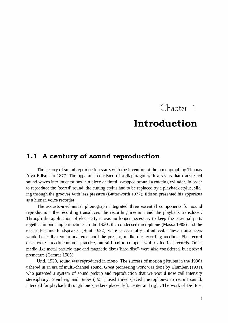
with rL and rR the distances to left and right loudspeaker. For sinusoidal signals SL and SR, an interference pattern is produced as shown in Figure 1.6. The wave fronts arriving at the listener's position are tilted towards the loudspeaker with the higher magnitude. Along the central axis (ahead of the listener), the interference pattern shows regions where the local form of the wave front is more or less the same as that of a single source somewhere between the -loudspeakers. There are, however, large phase transitions between neighboring regions, visible as light and dark shading. The width of the local wave fronts depends on the wavelength and the angle between the loudspeakers as seen from the listener's view-point: the further he moves away, the smaller the angle (at infinity this angle is zero and plane wave fronts will be received). difference: 0 dB difference: 6 dB
b. a.
Figure 1.6 Momentary pressure distribution in a 5×5 m2 area as a result of level differences between two loudspeakers (f = 400 Hz). The (momentary) phase is positive in the light regions, while it is negative in the dark
regions. Iso-phase lines are drawn at phase 0 and π (alternating) to indicate the orientation of the local wave fronts.

14 Chapter 1: Introduction
a. No level difference. b. The right loudspeaker has a 6 dB higher intensity level.
The frequency dependence and the angle of incidence (or direction of propagation) of the local wave front can be investigated for the listener position. Therefore, the exact expression for the phase function, calculated from (1.13), is taken. The angle of incidence ψ is now obtained from the phase difference between two receivers at x = x1 and x = x2 (Figure 1.7)
, (1.14)
with ∆x = x2 – x1 the spacing between the receivers. Note that this equation is exact for plane
waves with angular frequency ω, and still very accurate for spherical waves if the source
distance is larger than ∆x. Equation (1.14) is ambiguous for wavelengths smaller than the
spacing ∆x; these are not considered by restricting the angular frequency to ω < 2πc/∆x.
If ∆x = 17 cm is taken, the receivers may be thought of as ears. It should be noted, however, that (1.14) cannot be used to predict the actual image direction (as perceived by a listener) because it does not take into account wave diffraction around the head, and furthermore, no binaural localization model is incorporated. Nevertheless, it is a useful equation to gain insight in the (local) propagation direction of wave fronts.
The angle of incidence ψ is shown for four values of the interchannel intensity level difference in Figure 1.8. For low frequencies the image source direction is in agreement with (1.12). For higher frequencies the image direction collapses. This can be understood as follows. The width of the local wave fronts decreases with increasing frequency. For frequencies approaching f = c/ ∆x the receivers (`ears') will reach the borders of the local wave fronts.
Figure 1.7 The frequency-dependent angle of incidence is calculated from the phase difference between two receivers.

15
It is well known that the listening area for stereophony is restricted to the central axis. For listeners at off-axis locations the phantom source tends to shift towards the closest loudspeaker. It can be shown that there is a strong frequency dependence for the image direction as calculated from the phase differences between two receivers (centered off-axis). In Figure 1.9, Equation (1.14) has been applied for a position 0.5 m to the right of the sweet spot. For very low frequencies (f < 200 Hz) the receivers are still in the same local wave front region. For higher frequencies the phase relation between the receivers is unstable, as can be seen from the strong fluctuations of the image direction.
Figure 1.8 On-axis imaging with intensity stereophony. Position of receivers: 8.5 cm to the left and the right of the sweet spot.
Figure 1.9 Off-axis imaging with intensity stereophony. Position of receivers: 41.5 cm and 58.5 cm to the right of the sweet spot.
16 Chapter 1: Introduction
B. Time-based stereophony
If a small time delay is applied to the loudspeaker signals, a phantom source is heard towards the loudspeaker with the earliest signal. The imaging mechanism is based on the theory that the interaural time difference (ITD) is the main cue for directional hearing. For a real source, the maximal ITD (for a source 90º off-center) is approximately 0.7 ms. In other words, 0.7 ms is the largest natural signal delay between both ears. If two loudspeakers are used, with an increasing interchannel delay from 0 to 1.5 ms, the image will gradually move towards the earliest channel (Bartlett 1991). This effect is referred to as `summing localization' (Blauert 1983). If crosstalk from right loudspeaker to left ear and from left loudspeaker to right ear could be neglected, a delay of 0.7 ms would be enough to place the phantom image entirely to one side. Apparently, the resultant signals at the two ears suffer from crosstalk, and an exaggerated delay is necessary to shift the image to one loudspeaker.
For time-based stereophony, the perceived direction of the phantom image is strongly dependent on the source signal (Blauert 1983). If narrow band signals (1/3 octave band pulses and sinusoidal signals) are used, the direction of the image between the loudspeakers is not uniformly increasing with increasing delay time. This effect can also be heard with single tones in music reproduction: successive tones played at one instrument sometimes appear to come from different directions.
The effect is studied by looking at the reproduced wave field. Figure 1.10 displays the pressure distribution for an interchannel time difference of 0.5 ms and 1.0 ms. In comparison with Figure 1.6 it is clear that a time difference between the microphone signals leads to a shifted interference pattern. By further delaying the left channel, the pattern will shift until it is eventually returned to the starting-point.
Note that even for low frequencies the phase difference between the two receivers (`ears') on either side of the central axis can be high. This is illustrated in Figure 1.11 by applying Equation (1.14) for two receivers placed at either side of the sweet spot. The image direction suddenly blows up when the phase difference between the receivers is high. This behavior seems to be in agreement with the previously mentioned observations that localization of sinusoids suffers from divergence.
In general, the sound image produced by time-based stereophony does not correspond to a sound image heard in natural situations. The image direction varies from listener to listener, is affected by small head movements, and is quite signal dependent (Lipshitz 1986).

17
difference: 0.5 ms difference: 1.0 ms
b. a.
Figure 1.10 Momentary pressure distribution in a 5×5 m2 area as a result of time differences between two loudspeakers (f = 400 Hz). Contour lines are drawn at zero pressure for emphasis of wave fronts. a. 0.5 ms time difference. b. 1.0 ms time difference.
Figure 1.11 On-axis imaging with time-based stereophony. Position of receivers: 8.5 cm to the left and the right of the sweet spot.

18 Chapter 1: Introduction
1.6.3 Microphone and mixing techniques
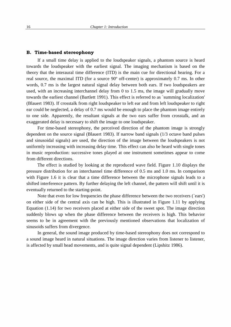
Microphones can be classified on the basis of their directivity characteristics. There are two main types of directivity patterns: omnidirectional and bidirectional (Figure 1.12). From these two, most other patterns can be constructed, e.g. the cardioid pattern is a sum pattern of the omnidirectional and bidirectional pattern. For stereophonic sound reproduction a set of two microphones is used to pick up the sound at some distance from the source(s). The configuration of these microphones and the appropriate distance to the sources is largely a matter of taste of the recording engineer, though a classification of microphone techniques, each with their own drawbacks and advantages, can be made. A thorough overview has been given by -Streicher et al. (1985) and Bartlett (1991). Only the main classes are described here: coincident pair, spaced pair and combined techniques.
Figure 1.12 Directivity patterns of commonly used microphones. a. Omnidirectional or pressure microphone. b.
Bidirectional or velocity microphone (with lobes in anti-phase). The pattern follows cos ϕ. c. Cardioid
microphone. The directivity pattern is given by ½ + ½ cos ϕ.
A. Coincident pair techniques
Two directional microphones are mounted closely to each other (nearly touching) while aiming at the left and right sides of the source area (Figure 1.13a). Intensity differences will arise, but phase differences between the signals are excluded. Therefore the method perfectly fits the requirements of intensity stereophony. The closer the source is to the axis of one of both microphones, the larger the intensity difference between the channels. A special form of coincident pair techniques is the Blumlein pair: two velocity microphones crossed at 90º, see Figure 1.14a. This technique was originally developed by Blumlein (1931) and is famous for its excellent localization properties.
19
Figure 1.13 Stereophonic microphone techniques. a. Coincident pair or XY-technique. b. Spaced pair or AB-technique.
The microphones signals of a Blumlein pair are given by
, (1.15a)
and
, (1.15b)
where S(ω) is the source signal and β the source angle. Note that the cosine factors represent the directivity of the velocity microphones. Clark et al. (1958) combined these signals to a formula for the intensity differen-ces at the left and right channel for the Blumlein pair:
. (1.16)
Finally, from (1.16) and the law of sines (1.12) it follows that stereophonic imaging with a Blumlein pair is described by
. (1.17)

20 Chapter 1: Introduction
Figure 1.14 a. A source at angle β is seen by a pair of crossed velocity microphones. b. Stereophonic imaging
with a Blumlein pair according to the `law of sines' (ϑ0 = 30º).
Figure 1.14b plots the true source direction b against the direction of the sound image ψ. Apparently, the Blumlein pair has fair imaging capabilities, though the images are slightly closer to the center than the true sources. In practice, a disadvantage of the used velocity microphones may be that they are equally senstive to sound from the rear as from the front. If the direct/reverberation ratio of the signals is to low, other directional microphones, such as cardioids can be used for intensity stereophony.
In most contemporary stereophonic recordings also spot microphones are used. In
addition to a main microphone pair, the signals of microphones close to the sources are recorded as well. For that purpose directional microphones are often used, but omnidirectional microphones may be preferred sometimes for sound quality reasons. The signals, that primarily contain the direct sound of one or a few sources, are added to the main microphone signals via a panoramic potentiometer circuit (pan pot) on the mixing console. This circuit distributes the signal energy between left and right channel. Therefore, imaging properties as described for coincident pair signals also apply for panned signals.
An advantage of the use of spot microphone signals is that the direct/reverberation ratio and the balance between various sources within the stereophonic image can be controlled better. The balancing engineer is able to add more direct sound if the image is too reverberant, or amplify the sound of one source in favor of others. Also, artificial reverberation or other signal manipulation can be used on spot microphone signals.

21
B. Spaced pair techniques
The second class of microphone techniques is the spaced pair or AB method. This method is appreciated for its ability to reproduce a spacious sound image. Two microphones, mostly with omnidirectional characteristics, are placed some distance d apart (Figure 1.13b). The sound from a source that is off-center has a different travel-time to each of the microphones. If a source is at a large distance compared to the distance d between the two pressure microphones, the pressure difference can be neglected, and the time delay to the farther microphone is the only signal difference. Imaging with a spaced pair technique is therefore described by the theory of time-based stereophony.
It has been argued yet, that an exaggeration of the applied time delays is necessary because of the situation during reproduction, where `crosstalk' from the loudspeakers to the opposite ears must be compensated. A second compensation is necessary due to the absence of a shielding head between the microphones during recording. Interaural level differences, that accompany the interaural time differences under natural circumstances, are missing. Except extra time delays, sometimes a shielding disc (Jecklin) or sphere is used in between the spaced microphones. This method is closely related to binaural recording and reproduction (Section 1.6.5).
Figure 1.15 The ORTF microphone technique uses two cardioids, angled 110º, and spaced by 17 cm.
C. Combined techniques
Various other stereophonic microphone techniques are employed. Most of them can be regarded as intermediates between coincident and spaced techniques. They attempt to combine the benefits of both classes while avoiding their disadvantages. An example is the ORTF system, originally designed by the French Broadcasting Organization (Figure 1.15). This system has been tuned to yield stable images with reasonable spaciousness. Subjective comparisons of stereophonic microphone techniques are given by Ceoen (1972) and Bartlett (1991).

22 Chapter 1: Introduction
1.6.4 Spectral properties of stereophony
Because two loudspeakers with correlated signals are used, stereophonic reproduction suffers from comb filter effects. In an anechoic environment, which, of course, is not a natural location for reproduction, the spectral distortion is easy to perceive. The thick line in Figure 1.16 shows the response at a receiver placed 8.5 cm to the right of the sweet spot for two identical signals fed to the loudspeakers. At 2.0 + 4.0n kHz (n is a positive integer) the left and right loudspeaker contributions are in anti-phase. If the receiver is moved 0.5 m to the right, much more notches occur, but they are less deep. Due to room reflections in a normal listening environment, the comb filter effects are partly masked by reflective sound.
Figure 1.16 Simulated stereophonic responses. Left and right loudspeaker are driven by identical signals. The receiver positions are 8.5 cm (thick line) and 58.5 cm (thin line) to the right of the sweet spot.
1.6.5 Binaural recording and reproduction
A special form of two-channel stereophony is binaural reproduction. During recording, two microphones are placed at the entrance of the ear canals of an artificial head. A headphone is used to reproduce the recorded sound. Binaural imaging is based on the assumption that a listener would perceive the same sound image whether he were present at the recording session or at the reproduction site, if the sound pressure at his eardrums in the latter situation is an exact copy of that in the former. It is not surprising that binaural reproduction can offer an extremely realistic 3D sound image.
A few disadvantages of binaural reproduction are mentioned here. When the head is moved (during playback), the recorded ear signals do not vary accordingly, which may violate

23
the realism of the sound image. A second objection is due to shape of the dummy torso and pinnae (shell of the ear). Because these external reflectors and diffractors may differ considerably from the listener's own torso and pinnae, the head related transfer functions (HRTFs) from source to dummy ears will differ from the listener's own HRTFs. Therefore, the perceived image may sound not as natural to all listeners. And finally, coloration of the binaural signals due to HRTFs will disqualify them for use with other reproduction techniques.
1.7 Surround sound systems
For a better understanding of current surround sound systems and the effort taken to remain compatible with two-channel stereophony, it is worthwhile to study the problems of quadraphony. Though commercially considered a fiasco, quadraphony used premises and principles that are still of interest.
1.7.1 Quadraphony
It was recognized that two loudspeakers were not able to re-create a true 3D image of the original sound field: sound coming from the sides, the back and above were lacking. If only the horizontal plane was considered, at least two loudspeakers were required to fill the gap (Figure 1.17a). This suggested that at least two more audio channels were necessary. However, not any extra playback channel would contribute as much to the total stereo image as the front loudspeakers: with each extra channel more redundancy was added. Moreover, compatibility with two-channel records was an important demand. A solution was therefore sought in matrix systems (Ten Kate 1993).
A matrix equation describes how the loudspeaker signals are related to the original
signals. Most quadraphonic proposals use a 4-2-4 scheme: four initial (studio) channels, two
Figure 1.17 a. Quadraphonic loudspeaker arrangement. b. Surround sound loudspeaker arrangement, such as used by Dolby Surround and some other systems.The surround signal S can be delayed by a few tens of milliseconds to ensure that sound is not localized at the surround loudspeakers.

24 Chapter 1: Introduction
transmission channels and four loudspeaker channels. Such systems consist of a 2×4 encoding matrix and a 4×2 decoding matrix. The transmission channels are encoded as
(1.18)
where LF , RF , LR and RR represent the signals of initial channels for left front, right front, left rear and right rear loudspeakers. The transmission channels must serve as reasonable two-channel reproduction channels for compatibility requirements. The quadraphonic loudspeaker channels, denoted with primes, are retrieved by the decoding scheme
. (1.19)
Power conservation yields for and for
. A 4×4 matrix results after substitution of (1.18) in (1.19). This matrix can be
optimized according to certain premises (Eargle 1971). Besides disagreement on the number of channels, also obscurity about the recording stra-
tegy and the aims to be achieved, caused a stagnation in the development of multi-channel surround (Gerzon 1977). At last, Dolby Laboratories introduced the Dolby Surround system. Being derived from their cinema surround sound standard Dolby Stereo, this domestic system became successful as well.
1.7.2 Dolby Surround
The Dolby Surround system uses a left, center, right and surround channel recovered from two transmission channels (Figure 1.17b). Such a configuration is appropriate if a television set is used in combination with audio channels. The central phantom image, as heard between left and right loudspeakers, is now anchored in the central loudspeaker. The transmission scheme is given by (Dressler 1993)
, (1.20)
with (or –3 dB) and j is a 90º phase shift. The loudspeaker signals are recovered as

25
. (1.21)
Crosstalk between adjacent channels is –3 dB, while it is –∞ dB between opposite channels. The S-signal is bandlimited from 100 Hz to 7 kHz, encoded with a modified Dolby B-type noise reduction and phase shifted over ± 90º. Since the crosstalk would lead to intolerable blurring of the image resolution (Bamford et al. 1995), additional active processing is done by a Pro Logic Decoder. The decoder detects the dominant direction in the playback channels and then applies enhancement in the same direction and in proportion to that dominance.
Compatibility with two-channel stereophony is supported to such an extent that a fairly satisfactory downmix is given. However, the harm done to stereophonic imaging by the encoding procedure is rather contrasting with the care taken in setting up an accurate stereophonic sound image (see Section 1.6).
1.7.3 Ambisonics
Ambisonics has its roots in quadraphonic matrixing (Cooper et al. 1972) and has been proposed as a successor of stereophony (e.g. Gerzon 1985 and Lipshitz 1986). Ambisonics uses a different microphone and imaging technique than stereophony. It pursues local wave front reconstruction: a listener at the sweet spot receives wave fronts that are copies of the original wave fronts. In this section a simple example is given with the following assumptions:
1. Analysis and reconstruction are restricted to a small area of the order of a wavelength. Therefore all incident waves in the original and the reproduced field may be considered to be plane waves.
2. Analysis and reconstruction are restricted to the horizontal plane.
3. Four loudspeakers are used for reconstruction.
4. Only the zeroth and first order spherical harmonics are taken into account. These can be measured with pressure and velocity microphones, respectively.
Only the first restriction is essential for ambisonic theory. The second and third
restriction are made here for simplicity in derivation, while the fourth restriction originates from the practical circumstance that second and higher order microphones have not been constructed yet.
Consider a plane wave with an angle of incidence ψ with respect to the x-axis (Figure 1.18a). Pressure and velocity at the origin are given by
, (1.22)

26 Chapter 1: Introduction
, (1.23a)
, (1.23b)
with P the pressure and V the velocity of the plane wave. Ambisonics uses a special microphone with nearly coincident diaphragms to acquire P, Vx and Vy. These signals can be encoded for transmission in so-called UHJ format (Gerzon 1985), and recovered at the reproduction site, where the loudspeaker inputs are calculated according to (Bamford et al. 1995)
(1.24)
with Ln the feed, and ϕn the direction of the nth loudspeaker, with N the total number of
loudspeakers, and ρ0c the acoustic impedance of a plane wave. For the arrangement shown in Figure 1.18b, loudspeaker signals (1.24) are evaluated as
, (1.25a)
, (1.25b)
, (1.25c)
. (1.25d)
Figure 1.18 Ambisonic reproduction example. a. Plane wave incidence at origin. b. Reconstruction of the plane wave by composition with loudspeakers.

27
The reconstructed wave at the origin is found by superposition of the loudspeaker outputs. The pressure is given by summation of all contributions
, (1.26)
and the velocity by summing x and y components (note that opposite loudspeakers have opposite signs for their velocity components)
, (1.27a)
. (1.27b)
Though in theory the original pressure and velocity are fully recovered, problems may arise due to the prescription that opposite loudspeakers have anti-phased velocity information. Certainly such cancelation is very critical, and will probably require careful adjustment of the decoding circuitry and accurate positioning of loudspeakers. At high frequency, moreover, cancelation of oppositely propagating waves will not occur at all, because firstly, there is a delay between left and right waves at the listener's ears, and secondly, the head shields the wave field.
1.7.4 Surround sound in the cinema
The first surround sound project in motion picture industry has been Disney's discrete six-channel Fantasia in 1941. Since then, various systems have been designed, of which Dolby Stereo has been most successful. This surround sound system decodes two channels from 35 mm optical prints into left (L), center (C), right (R) and surround (S) loudspeaker channels. It is the professional version of the Dolby Surround system, as described in section 1.7.2.
In the 1990s, the digital era in cinema was entered with three non-compatible digital surround sound systems: Dolby Stereo Digital, Digital Theater Systems and Sony Dynamic Digital Sound (Blake 1995). All systems employ the so-called 5.1 format: a discrete six-channel configuration with L-C-R-S1-S2 and a subwoofer channel (Figure 1.19). For cinemas with less than five loudspeaker clusters, also a three-channel or four-channel sub-set can be decoded from the 5.1 format. On the other hand, extensions up to the 7.1 format are supported as well (see Figure 1.19).

28 Chapter 1: Introduction
Figure 1.19 Surround sound configurations. The S1´ and S2´ surround loudspeakers are optional. a. The 5.1 surround sound format. b. The 7.1 surround sound format.
1.7.5 Discrete surround sound at home
With the arrival of advanced widescreen television, new opportunities for the audio industry were provided. A recommendation of the ITU-R (1991) committee has standardized multi-channel transmission formats and loudspeaker arrangements. The transmission format is 5.1 (five wide band channels and one narrow band subwoofer channel) with three front channels and two surround channels (denoted as 3/2) as to be compatible with motion picture formats and arrangements. Also, sub-sets of this configuration are possible, such as 3/1, as used by Dolby Surround, and 2/0, which is the conventional two-channel stereophony. Others propose the use of side surround loudspeakers, S1´ and S2´ in Figure 1.19, because the imaging of lateral sources and reflections is problematic with only front and rear loudspeakers (Griesinger 1996 and Zieglmeier et al. 1996).
Preparation of audio signals for the 3/2 system is largely an extension of stereophonic imaging. Reports on recordings for the new standard mention conventional microphone techniques. Schneider (1996) reports that a conventional AB pair could not provide a satisfactory pan pot mix for the frontal channels L, C and R. Finally, three discrete microphone signals, with 3 dB attenuation for the central channel, were used for these channels to image a symphony orchestra. Spikofski et al. (1992) propose a reversed ORTF-pair (Figure 1.20a) for the surround channels. Theile (1996) uses a similar microphone configuration for overall sound pick-up (Figure 1.20b). He argues that the center channel should be ignored as long as no adequate three-channel main microphone exists, leaving a 2/2 configuration.

29
Figure 1.20 a. ORTF-pair used for surround sound pick-up. b. Modified ORTF-pairs for a 2/2 system.
1.8 Conclusions
Since the early 1970s, the audio industry is vainly trying to enrapture the public for multi-channel reproduction. The motivation for these efforts was the general idea that the listener should be enveloped with sound, as in natural sound fields. However, sound reproduction and two-channel stereophony are still synonymous to the consumer. The commercial failure of multi-channel sound so far, is regarded to be caused by moderate enhancement of sound quality and lack of standardization.
It is believed that these problems have been overcome by digital technology and a standardized surround format, the so-called 3/2 format. Though presented as an innovative solution, the new surround sound proposals still lean heavily on stereophonic imaging. Therefore, important drawbacks of stereophony will unavoidably be adopted as well.
In this chapter, a reformulation of the aims and requirements for sound reproduction has been given. It is shown that stereophony cannot fulfill such demands: imaging is restricted to an extremely narrow listening area. Outside this area, spatial and temporal distortion of the sound image occurs. The main goal of the present research is to develop a method of sound reproduction that offers a natural high quality sound image in a large listening area.

30 Chapter 1: Introduction

31
Chapter 2
Wave Field Synthesis
2.1 Introduction
This chapter gives the theoretical basis for spatially correct sound reproduction by apply-ing the concept of wave field synthesis (Berkhout 1988 and Berkhout et al. 1993). It will beshown that – starting from the Kirchhoff-Helmholtz wave field representation – a synthesisoperator can be derived that allows for a spatial and temporal reconstruction of the originalwave field. The general 3D-solution (Section 2.2) can be transformed into a so-called 2½D-solution (Section 2.3), which is sufficient for reconstructing the original sound field in the(horizontal) plane of listening. For that purpose a linear array of loudspeakers is used to gener-ate the sound field of virtual sources lying behind the array. A special manifestation of theoperator appears in the case that sources in front of the array need to be synthesized. In thatcase, the array radiates convergent waves towards a focus point, from which divergent wavespropagate into the listening area (Section 2.3.2).
For finite or corner-shaped arrays diffraction occurs. In most situations diffraction wavescause no serious distortion of the perceived sound image. However, if the main contribution ofthe wave at a certain listening position is generated near a discontinuity of the array, diffractioncan have audible effects. Solutions for diffraction are offered in Section 2.4.
Discretization of continuous source distributions has influence on the frequencyresponse and the spatial behavior of the synthesized wave field. Section 2.5 discusses artefactsand solutions. Finally, related research in the field of wave field synthesis is summarized inSection 2.6.

32 Chapter 2: Wave Field Synthesis
2.2 Kirchhoff-Helmholtz Integral
From Green’s theorem and the wave equation, the Kirchhoff-Helmholtz integral can bederived for the pressure PA at a point A within a closed surface S (e.g. Skudrzyk 1954 or Berk-hout 1982)
, (2.1)
where G is called the Green’s function, P is the pressure at the surface caused by an arbitrarysource distribution outside the enclosure, and n is the inward pointing normal unit vector to thesurface, see Figure 2.1. G should obey the inhomogeneous wave equation for a monopolesource at position A
. (2.2)
The general form of the Green’s function is given by
, (2.3)
where F may be any function satisfying the wave equation (2.2) with the right-hand term set tozero. For the derivation of the Kirchhoff integral F = 0 is chosen, and the space variable r ischosen with respect to A
. (2.4)
Thus G represents the wave field of a point source in A. The physical interpretation ofthese choices is that a fictitious point source must be placed in A to determine the acoustical
PA1
4π------ P G G P∇–∇( )n Sd
S∫=
G2
k2G+∇ 4πδ r r A–( )–=
nϕ
A
S
Figure 2.1 The pressure in a point A can be calculated if the wave field of an external source distribution is knownat the surface of a source-free volume containing A.
r
Gjkr–( )exp
r------------------------- F+=
r x xA–( )2y yA–( )2
z zA–( )+ +2
=

2.2 Kirchhoff-Helmholtz Integral 33
transmission paths from the surface towards A. Substitution of the solution for G and the equa-tion of motion
(2.5)
into integral (2.1) finally leads to the Kirchhoff integral for homogeneous media
. (2.6)
The first term of the integrand of (2.6) represents a dipole source distribution driven with thestrength of the pressure P at the surface, while the second term represents a monopole sourcedistribution driven with the normal component of the particle velocity Vn at the surface (Figure2.2). The original source distribution may be called the primary source distribution; the mono-pole and dipole sources may be called the secondary source distribution.
Since A can be anywhere within the volume enclosed by S, the wave field within that
volume is completely determined by (2.6), whereas the integral is identically zero outside theenclosure. This can be understood in an intuitive manner by considering that the positive lobesof the dipoles interfere constructively with the monopoles inside the surface, while the nega-tive lobes of the dipoles exactly cancel the single positive lobe of the monopoles (see also Fig-ure 1.12) outside the surface. Apparently, part of the complexity of the Kirchhoff expression isinvolved in canceling the wave field of the secondary sources outside the closed surface. Forthe application of the Kirchhoff integral in wave field synthesis, this cancelation property is ofless importance. Therefore, two special solutions of the Green’s function are chosen that willconsiderably simplify the Kirchhoff integral, be it at the cost of a fixed surface geometry and a
n∂∂P
jωρ0Vn–=
PA1
4π------ P1 jkr+
r2
---------------- ϕ jkr–( )expcos jωρ0Vn
jkr–( )expr
------------------------- + Sd
S∫=
A
S
Figure 2.2 The pressure in a point A can be synthesized by a monopole and dipole source distribution at a surfaceS. The strength of the distributions depends on the velocity and pressure of external sources measured at the sur-face.
+
+
+++
++
+
+
++
+
+
++
++
--
-
-
-
-
-
--
- -
--
- --
++
+
+
++
++
++ +
++
+
+

34 Chapter 2: Wave Field Synthesis
non-zero wave field outside the closed surface. Of course, the wave field inside the closed sur-face is correctly described by these solutions, known as the Rayleigh I and II integrals.
2.2.1 Rayleigh I integral
The Rayleigh I integral can be found by choosing a particular surface of integration forintegral (2.1) and a suitable function F in (2.3). The surface consists of a plane at z = 0 and ahemisphere in the half space z > 0, as drawn in Figure 2.3. All sources are located in the halfspace z < 0, so for any value of the radius R the volume enclosed by S1 and S2 is source-free. IfG(r) falls off faster than or proportional to 1/r, the Sommerfeld condition is satisfied and theintegral over this part of the surface vanishes for . The pressure in A is now found bysubstitution of (2.3) in integral (2.1):
, (2.7)
where S1 is the infinite plane surface at z = 0.
The aim is to choose a function F that causes the first term of the integrand to vanish. Forthat to be true, the normal component of the gradient of F should have a sign opposite to that ofthe normal component of the gradient of . This will be the case for
(2.8)
which is the pressure of a monopole at A', the image of A mirrored in the plane S1. On S1, r' = r
R ∞→
PA1
4π------ P
n∂∂ jkr–( )exp
r------------------------- F+
jkr–( )expr
------------------------- F+n∂
∂P–
Sd
S1
∫=
n
ϕ
A
S2
zx
n
r' r R
S1
A'
Figure 2.3 The integral for the Rayleigh representations runs over a hemisphere surface S2 and a plane surface S1.
primary source
z < 0 z > 0
distribution
jkr–( )exp r⁄
Fjkr'–( )exp
r'--------------------------=

2.2 Kirchhoff-Helmholtz Integral 35
applies and therefore
, (2.9)
which causes the first term of the integrand of (2.7) to vanish indeed, yielding the Rayleigh Iintegral after substitution of (2.5)
. (2.10)
This equation states that a monopole distribution in the plane z = 0, driven by two times thestrength of the particle velocity components perpendicular to the surface, can synthesize thewave field in the half space z > 0 of a primary source distribution located somewhere in the otherhalf space z < 0 (see Figure 2.4).
Note that such a distribution of monopoles will radiate a ‘mirror’ wave field into the halfspace z < 0, since there are no dipoles to cancel this wave field. Therefore the Rayleigh I solu-tion can be applied for synthesis if the wave field in the half space z < 0 is of no interest.
n∂∂F
r'∂∂ jkr'–( )exp
r'--------------------------
r'∂n∂------=
= r∂
∂ jkr–( )expr
-------------------------r∂–
n∂--------
n∂
∂ jkr–( )expr
-------------------------–=
PA1
2π------ jωρ0Vnjkr–( )exp
r------------------------- Sd
S1
∫=
Figure 2.4 With the aid of the Rayleigh I integral the wave field of a primary source distribution can be synthesizedby a monopole distribution at z = 0 if the velocity at that plane is known.
primary sources
z = 0
+
+
+
+
+
+
+
z < 0 z > 0
secondary sources

36 Chapter 2: Wave Field Synthesis
2.2.2 Rayleigh II integral
In order to find the Rayleigh II solution, a function F is required that will eliminate thesecond term of (2.7). The situation as depicted in Figure 2.3 is considered again. A choice
(2.11)
will obviously have the desired effect, because at the plane of integration r' = r applies, causingthe second term of (2.7) to disappear. This time, G represents the wave field of a monopole atA, together with an anti-phase monopole at A'. The Rayleigh II integral can now be derived as
. (2.12)
This expression states that the wave field in the half space z > 0 can be synthesized by a distri-bution of dipoles, driven by two times the strength of the pressure (measured at z = 0) of a sourcedistribution in the half space z < 0 (Figure 2.5). Note that such a distribution of dipoles will ra-diate a ‘mirror’ wave field into the half space z < 0, the pressure of which is in anti-phase withthe pressure at z > 0.
2.3 Synthesis operator for line distributions
In principle, the Rayleigh I and II integrals can be used to synthesize the wave field ofany primary source distribution by a planar array of loudspeakers. The discretization of theoperators, from a continuous distribution of secondary sources to a discrete array of loud-speakers, will be treated in Section 2.5. In this section an intermediate step is made, from pla-
Fjkr'–( )exp
r'--------------------------–=
PA1
2π------ P
1 jkr+
r2
---------------- ϕcos jkr–( )exp SdS1
∫=
Figure 2.5 With the aid of the Rayleigh II integral the wave field of a primary source distribution can be synthe-sized by a dipole distribution at z = 0 if the pressure at that plane is known.
primary sources
z = 0
z < 0 z > 0
+ -
+ -
+ -
+ -
+ -
+ -
secondary sources

2.3 Synthesis operator for line distributions 37
nar to linear distributions. Such a reduction of dimensions is allowed as long as therequirements for spatial sound reproduction are being respected (Section 1.5).
A derivation of the Rayleigh I and II integrals in two dimensions (abbreviated: 2D) isgiven by Berkhout (1982). Analogously to the 3D situation, the wave field of a primary sourcedistribution can be represented by a distribution of secondary sources at a straight line. How-ever, the 2D analogy of a secondary point source behaves as a line source in 3D, i.e. instead ofthe -law, a -law is followed. Such solutions are of little practical value for wavefield synthesis. Therefore, Vogel (1993) has proposed a different approach, resulting in anexpression for a so-called 2½D-operator. This operator can be regarded as an intermediateform between the 3D and 2D Rayleigh operators, because the secondary sources have 1/r-attenuation while the derivation is given in a plane.
De Vries (1996) assumed monopole characteristics for the primary source and incorpo-rated arbitrary directivity characteristics of the secondary sources (loudspeakers) in the synthe-sis operator. He showed that the characteristics of the secondary sources and the primarysource are inversely interchangeable. Furthermore, his simulations show that if the directivitypatterns of one or more array loudspeakers deviate from the others, serious synthesis errorsmay occur. Therefore all secondary sources should have identical characteristics. The deriva-tion given here starts off with arbitrary characteristics for the primary source, and monopolecharacteristics for the secondary sources. It follows the treatment given by Start (1996), whoderived an expression for the 2½D-operator by reducing the (exact) 3D Rayleigh I surface inte-gral to a line integral.
The position of the primary source is not restricted to the half plane behind the secondaryline source, as will be shown in Section 2.3.2. The presence of sources in front of the loud-speaker arrays may contribute strongly to the imagination of the listener.
A summary and generalization of 2½D-operators is given in Section 2.3.3.
2.3.1 2½D Synthesis operator
Consider a primary source S in the xz-plane, as drawn in Figure 2.6. The pressure field ofthe primary source will be given by
, (2.13)
where S(ω) is the source function and G(ϕ, ϑ, ω) is the directivity characteristic of the sourcein the far-field approximation ( kr >> 1 ). Across the xy-plane, a secondary source distributionwith monopole characteristics is situated, which will synthesize the wave field of the primarysource at the receiver position R according to the Rayleigh I integral (2.10)
(2.14)
with Vn(r, ω) the velocity component of the primary source perpendicular to the xy-plane. The
1 r⁄ 1 r⁄
P r ω,( ) S ω( )G ϕ ϑ ω, ,( ) jkr–( )expr
-------------------------=
Psynth1
2π------ jωρ0Vn r ω,( ) jk∆r–( )exp∆r
----------------------------- xd ydxy-plane∫=

38 Chapter 2: Wave Field Synthesis
surface integral will be reduced to a line integral along the x-axis by evaluating the integral inthe y direction along the line m. By applying the equation of motion (2.5) to Equation (2.13) itfollows that
. (2.15)
In the chosen geometry of Figure 2.6, with ϕ = atan ( x/z ) and ϑ = atan ( y/ ), this ex-pression is written as
. (2.16)
The integration along the line m can be carried out by applying the stationary phase method(Bleistein 1984). This method is concerned with integrals of the form
. (2.17)
Equation (2.14), with substitution of (2.16), indeed takes this form. The amplitude part is
z
xy
Figure 2.6 The Rayleigh I integral is evaluated for a primary source S and receiver R, both located in the xz-plane.Vector r points from the primary source to a secondary source M at the line m. Vector ∆r points from secondarysource to receiver. The projections on the xz-plane are denoted by subscript 0.
∆r
R
M
m
∆r0
S
r0
ϕϑ
r
jωρ0Vn r ω,( )n∂
∂ P– S ω( )–
z∂∂
G ϕ ϑ ω, ,( ) jkr–( )expr
-------------------------= =
x2 z2+
jωρ0Vn r ω,( ) S ω( ) jkr–( )expr
-------------------------ϕsin
r ϑcos---------------
G∂ϕ∂-------
ϕ ϑsincosr
------------------------G∂ϑ∂-------
1 jkr+r
----------------G ϕ ϑcoscos+ +
=
I f y( ) jφ y( )( )exp yd∞–
∞
∫=

2.3 Synthesis operator for line distributions 39
, (2.18a)
in which the variables ϑ, r and ∆r implicitly depend on y, while the phase is given by
. (2.18b)
For φ >> 1, the approximate solution to (2.17) is
, (2.19)
where y0 is the stationary phase point and φ"(y0) the second derivative of φ evaluated at y0. Thestationary phase point is defined as the point where φ(y) reaches its stationary value, i.e. whereφ'(y) = 0. From inspection of Figure 2.6 it follows that
, (2.20a)
(and therefore ϑ0 = 0),
, (2.20b)
, (2.20c)
. (2.20d)
For kr0 >> 1, the second term of f(y0) is dominating, and therefore (2.14) is finally reduced to
. (2.21)
Integral (2.21) states that the contributions of all secondary sources M along the line m can beapproximated by the contribution of a secondary point source at the intersection of m with thex-axis. The driving function Qm(x, ω) of that secondary monopole point source at x is
, (2.22a)
yielding for the integral (2.21)
f y( ) 12π------
S ω( )r∆r------------
ϕsinr ϑcos---------------
G∂ϕ∂-------
ϕ ϑsincosr
------------------------G∂ϑ∂-------
1 jkr+r
----------------G ϕ ϑcoscos+ +
=
φ y( ) k r ∆r+( )–=
I f y0( ) jφ y0( )( ) 2πjφ″ y0( )----------------exp≈
y0 0=
φ y0( ) k r0 ∆r0+( )–=
φ″ y0( ) kr0 ∆r0+
r0∆r0--------------------–=
f y0( ) 12π------
S ω( )r0∆r0--------------
ϕsinr0
-----------G ϕ 0 ω, ,( )∂
ϕ∂-----------------------------
1 jkr0+
r0-------------------G ϕ 0 ω, ,( ) ϕcos+
=
Psynth S ω( ) jk2π------
∆r0
r0 ∆r0+--------------------
∞–
∞
∫ G ϕ 0 ω, ,( ) ϕjkr0–( )exp
r0
---------------------------jk∆r0–( )exp
∆r0-------------------------------dxcos=
Qm x ω,( ) S ω( ) jk2π------
∆rr ∆r+---------------G ϕ 0 ω, ,( ) ϕcos
jkr–( )exp
r-------------------------=

40 Chapter 2: Wave Field Synthesis
, (2.22b)
in which the subscripts of the variables r0 and ∆r0 have been dropped for convenience.It will be verified here that the obtained driving function is valid within the approxima-
tions of the stationary phase method. Therefore this method is applied to integral (2.22b). Thistime, the amplitude f(x) and phase φ(x) function are
(2.23a)
and
(2.23b)
respectively, in which ϕ, r and ∆r are implicitly dependent on x. Again a stationary phase pointhas to be found. From Figure 2.7 it is obvious that it lies at the intersection of the line RS withthe x-axis. Introducing ρ as the vector pointing from primary source to stationary phase point,the second derivative of the phase function of the integrand of (2.21) is found as
, (2.24)
where z0 and ∆z0 are the respective distances (positive) of the primary source and the receiverto the x-axis. The amplitude part of the integrand, evaluated at the stationary phase point, yields
. (2.25)
Realizing that cos ϕ0 = (z0 + ∆z0)/(ρ + ∆ρ), substitution of (2.24) and (2.25) into (2.19) gives
. (2.26)
Comparison of this expression with the true wave field (2.13) shows that the synthesized wavefield is equal to the true wave field of the primary source within the plane containing this sourceand the distribution of secondary sources. Now consider the situation of different receiver points
Psynth Qm x ω,( )∞–
∞
∫jk∆r–( )exp
∆r-----------------------------dx=
f x( ) S ω( )∆r r-------------
jk2π------
∆rr ∆r+---------------G ϕ 0 ω, ,( ) ϕcos=
φ x( ) k r ∆r+( )–=
φ″ x0( ) kz0
2
ρ3-------–
z0 ∆z0+
∆z0-------------------- =
f x0( ) S ω( )∆ρ ρ---------------
jk2π------
∆z0
z0 ∆z0+--------------------G ϕ0 0 ω, ,( ) ϕ0cos=
Psynth S ω( )G ϕ0 0 ω, ,( ) jk ρ ∆ρ+( )–( )expρ ∆ρ+( )--------------------------------------------=
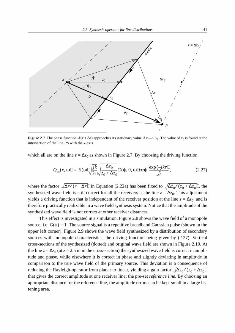
2.3 Synthesis operator for line distributions 41
which all are on the line z = ∆z0 as shown in Figure 2.7. By choosing the driving function
, (2.27)
where the factor in Equation (2.22a) has been fixed to , thesynthesized wave field is still correct for all the receivers at the line z = ∆z0. This adjustmentyields a driving function that is independent of the receiver position at the line z = ∆z0, and istherefore practically realizable in a wave field synthesis system. Notice that the amplitude of thesynthesized wave field is not correct at other receiver distances.
This effect is investigated in a simulation. Figure 2.8 shows the wave field of a monopolesource, i.e. G(ϕ) = 1. The source signal is a repetitive broadband Gaussian pulse (shown in theupper left corner). Figure 2.9 shows the wave field synthesized by a distribution of secondarysources with monopole characteristics, the driving function being given by (2.27). Verticalcross-sections of the synthesized (dotted) and original wave field are shown in Figure 2.10. Atthe line z = ∆z0 (at z = 2.5 m in the cross-section) the synthesized wave field is correct in ampli-tude and phase, while elsewhere it is correct in phase and slightly deviating in amplitude incomparison to the true wave field of the primary source. This deviation is a consequence ofreducing the Rayleigh-operator from planar to linear, yielding a gain factor that gives the correct amplitude at one receiver line: the pre-set reference line. By choosing anappropriate distance for the reference line, the amplitude errors can be kept small in a large lis-tening area.
Figure 2.7 The phase function -k(r + ∆r) approaches its stationary value if x —> x0. The value of x0 is found at theintersection of the line RS with the x-axis.
x-ax
is
ρ
∆ρ
R
S
x0
∆r
r
z0 ∆z0
ϕ0
z = ∆z0
ϕ
Qm x ω,( ) S ω( ) jk2π------
∆z0
z0 ∆z0+--------------------G ϕ 0 ω, ,( ) ϕcos
jkr–( )exp
r-------------------------=
∆r r ∆r+( )⁄ ∆z0 z0 ∆z0+( )⁄
∆z0 z0 ∆z0+( )⁄

42 Chapter 2: Wave Field Synthesis
Gaussian pulse
Figure 2.8 Wave field of a pulsating monopole source. The arrows indicate the position of the cross-section shownin Figure 2.10.
+++++++++++++++++++++++++++++++++++++++++++++++z = 0
z = ∆z0
Figure 2.9 A line distribution of secondary monopole sources synthesizes the wave field of a pulsating monopolesource.The arrows indicate the position of the cross-section shown in Figure 2.10.
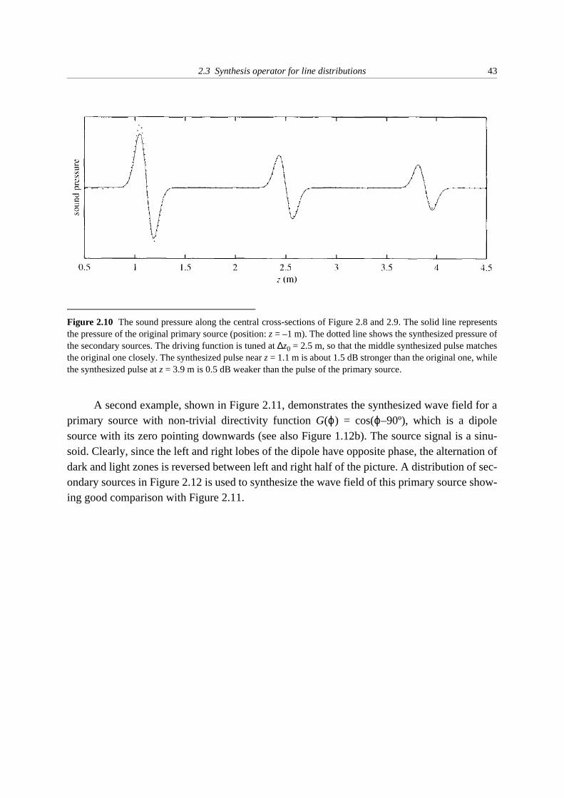
2.3 Synthesis operator for line distributions 43
A second example, shown in Figure 2.11, demonstrates the synthesized wave field for aprimary source with non-trivial directivity function G(ϕ) = cos(ϕ–90º), which is a dipolesource with its zero pointing downwards (see also Figure 1.12b). The source signal is a sinu-soid. Clearly, since the left and right lobes of the dipole have opposite phase, the alternation ofdark and light zones is reversed between left and right half of the picture. A distribution of sec-ondary sources in Figure 2.12 is used to synthesize the wave field of this primary source show-ing good comparison with Figure 2.11.
Figure 2.10 The sound pressure along the central cross-sections of Figure 2.8 and 2.9. The solid line representsthe pressure of the original primary source (position: z = –1 m). The dotted line shows the synthesized pressure ofthe secondary sources. The driving function is tuned at ∆z0 = 2.5 m, so that the middle synthesized pulse matchesthe original one closely. The synthesized pulse near z = 1.1 m is about 1.5 dB stronger than the original one, whilethe synthesized pulse at z = 3.9 m is 0.5 dB weaker than the pulse of the primary source.
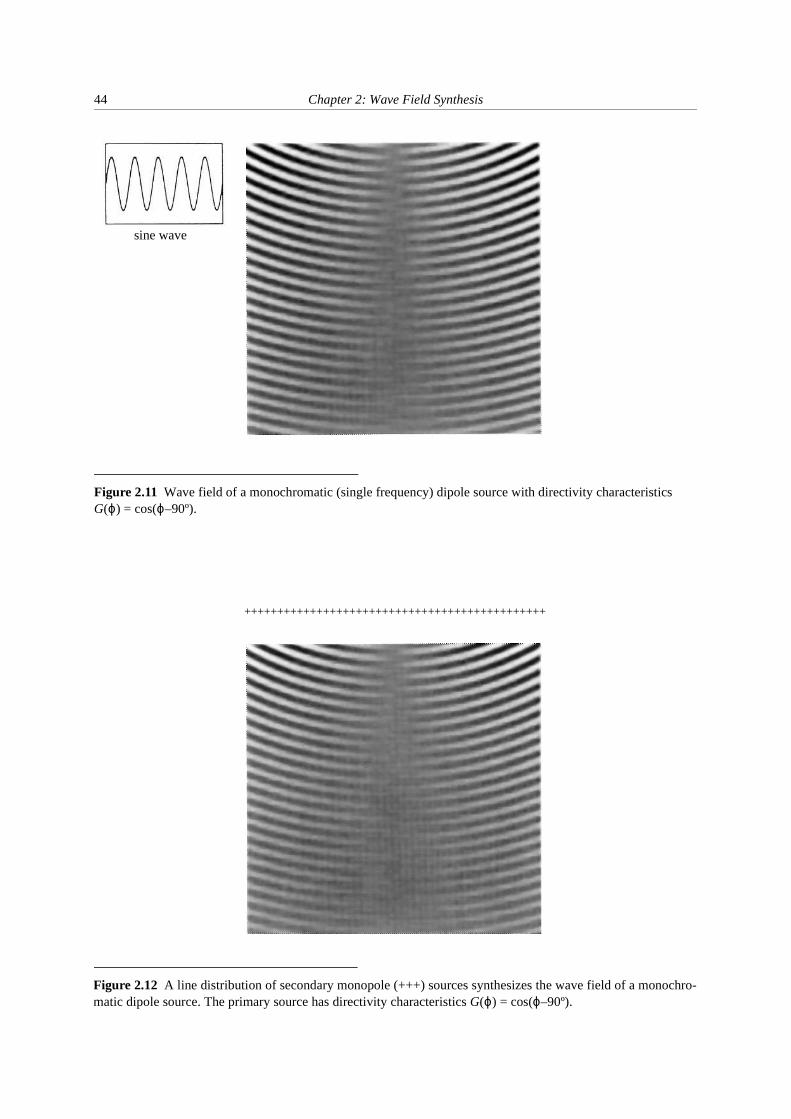
44 Chapter 2: Wave Field Synthesis
sine wave
Figure 2.11 Wave field of a monochromatic (single frequency) dipole source with directivity characteristics G(ϕ) = cos(ϕ–90º).
Figure 2.12 A line distribution of secondary monopole (+++) sources synthesizes the wave field of a monochro-matic dipole source. The primary source has directivity characteristics G(ϕ) = cos(ϕ–90º).
++++++++++++++++++++++++++++++++++++++++++++++

2.3 Synthesis operator for line distributions 45
Instead of a distribution of monopole sources, also dipole sources can be used to synthe-sized a wave field. Starting from the Rayleigh II formulation (2.12), it can be shown analo-gously to the derivation of the monopole driving function that in this case the synthesizedwave field is equal to
(2.28a)
where ψ is the angle between the normal n (to the secondary source line) and the direction ofthe receiver (see Figure 2.13). Qd is the dipole driving function given by
, (2.28b)
where z0 and ∆z0 are the respective distances of S and R to the x-axis.
2.3.2 Focusing operator
From the principle of reciprocity between source and receiver, which states that theacoustic transmission paths are reversible, it is obvious that it must be possible to focus soundwaves from a distribution of secondary sources towards a focus point. Focusing of sound isapplied in seismic data processing (Berkhout 1997b and Thorbecke 1997) and in ultrasonicscanning of human tissues. Focusing of sound also appears in nature: in outdoor sound propa-gation, so-called caustic surfaces may occur if sound waves are affected by wind gradients(Pierce 1991).
Psynth Qd x ω,( )∞–
∞
∫ jk ψ jk∆r–( )exp∆r
-----------------------------cos dx=
Qd x ω,( ) S ω( ) 12πjk-----------
∆z0
z0 ∆z0+--------------------G ϕ 0 ω, ,( ) jkr–( )exp
r-------------------------=
Figure 2.13 The wave field of a primary source can be synthesized by a secondary dipole source distribution alongthe x-axis.
R
S
∆rr
z0 ∆z0
ϕ
ψ+−
x-axis
n
referenceline

46 Chapter 2: Wave Field Synthesis
A 2½D focusing operator can be derived for a secondary source distribution along astraight line. From inspection of the geometry of Figure 2.14, with the secondary sources at z =0 and both the primary source and the receiver line at z > 0, it is clear that the waves of the pri-mary source are propagating in the direction opposite to the waves of the secondary sources inthe dark area where 0 < z < z0. In the space z > z0, the waves of the primary source and thewaves of the secondary sources are traveling in positive z-direction. In that area, a reconstruc-tion of the primary wave field by a distribution of secondary monopole or dipole sources ispossible, as shown in Appendix A. The synthesized wave field for a distribution of secondarymonopole sources is given by (A.3)
(2.29a)
with driving function (A.15)
. (2.29b)
Figure 2.15 displays the wave field of a focusing secondary source distribution. In thearea z < z0, the waves are convergent towards the focus (concave wave fronts). Figure 2.16shows a cross-section through the focus. Note the change of the waveform at the focus, whichis quantified by Equation (A.22): the phase of the waves is shifted by 90º when passing thefocus.
Figure 2.14 The wave field of a primary source S is synthesized at the reference line by secondary sources at z = 0.
R
∆r
∆z0
Sr
ϕ
z
xy
M
z = 0
ρ
z0
referenceline
Psynth Qmfoc
x ω,( ) jk∆r–( )exp∆r
----------------------------- xd∞–
∞
∫=
Qmfoc
x ω,( ) S ω( ) k2πj--------
∆z0
∆z0 z0–------------------- ϕ +jkr( )exp
r-------------------------cos=

2.3 Synthesis operator for line distributions 47
Figure 2.15 Wave field of a focusing monopole distribution. The source signal is a repetitive pulse. The arrowsindicate the position of the cross-section shown in Figure 2.16.
+++++++++++++++++++++++++++++++++++++++++++++++
z = z0
Figure 2.16 Cross-section of the wave field of Figure 2.15. The position of the primary source (focus) is at z0 =1.5 m.
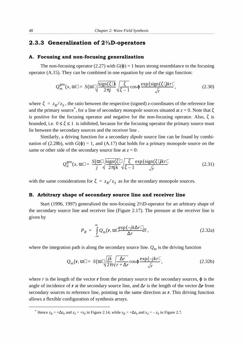
48 Chapter 2: Wave Field Synthesis
2.3.3 Generalization of 2½D-operators
A. Focusing and non-focusing generalization
The non-focusing operator (2.27) with G(ϕ) = 1 bears strong resemblance to the focusingoperator (A.15). They can be combined in one equation by use of the sign function:
, (2.30)
where , the ratio between the respective (signed) z-coordinates of the reference lineand the primary source* , for a line of secondary monopole sources situated at z = 0. Note that ζis positive for the focusing operator and negative for the non-focusing operator. Also, ζ isbounded, i.e. is inhibited, because for the focusing operator the primary source mustlie between the secondary sources and the receiver line .
Similarly, a driving function for a secondary dipole source line can be found by combi-nation of (2.28b), with G(ϕ) = 1, and (A.17) that holds for a primary monopole source on thesame or other side of the secondary source line at z = 0:
(2.31)
with the same considerations for as for the secondary monopole sources.
B. Arbitrary shape of secondary source line and receiver line
Start (1996, 1997) generalized the non-focusing 2½D-operator for an arbitrary shape ofthe secondary source line and receiver line (Figure 2.17). The pressure at the receiver line isgiven by
, (2.32a)
where the integration path is along the secondary source line. Qm is the driving function
, (2.32b)
where r is the length of the vector r from the primary source to the secondary sources, ϕ is theangle of incidence of r at the secondary source line, and ∆r is the length of the vector ∆r fromsecondary sources to reference line, pointing in the same direction as r. This driving functionallows a flexible configuration of synthesis arrays.
* Hence zR = +∆z0 and zS = +z0 in Figure 2.14, while zR = +∆z0 and zS = – z0 in Figure 2.7.
Qmgen
x ω,( ) S ω( ) sign ζ( )k2πj
---------------------ζ
ζ 1–----------- ϕ sign ζ( )jkr( )exp
r----------------------------------------cos=
ζ zR zS⁄=
0 ζ 1≤ ≤
Qdgen
x ω,( ) S ω( )j
------------sign ζ( )2πjk
------------------ζ
ζ 1–-----------
sign ζ( ) jkr( )exp
r----------------------------------------=
ζ zR zS⁄=
PR Qm r ω,( )∞–
∞
∫jk∆r–( )exp
∆r-----------------------------dl=
Qm r ω,( ) S ω( ) jk2π------
∆rr ∆r+--------------- ϕcos
jkr–( )exp
r-------------------------=

2.3 Synthesis operator for line distributions 49
In case of an arbitrarily shaped line of secondary dipoles, the synthesis integral reads
(2.33a)
with
. (2.33b)
Angle ψ is defined as in (2.28a) and depicted in Figure 2.13. For the stationary phase point therelation ψ = ϕ applies.
C. Remark
It seems plausible to generalize driving function (2.30) for a smooth curvature of thereceiver line and the secondary source line by setting as in (2.32b), thus extendingthe validity of (2.32b) to focused primary sources. Because ∆r and r are lengths of vectorsrather than signed coordinates, a sign has to be implemented in ζ artificially, if the secondarysource line is not straight as for driving function (2.30). In this way the synthesis operator isable to discriminate between focusing and non-focusing situations. From symmetry and reci-procity (and simulation results) such a generalization appears reasonable.
Figure 2.17 Synthesis with a curved secondary source line and reference line is allowed as long as each point Ron the reference line ‘sees’ only one stationary phase point on the secondary source line.
R
S r
∆r
secondary referenceline
source line
dl
ϕ
PR Qd r ω,( )∞–
∞
∫ jk ψ jk∆r–( )exp∆r
-----------------------------cos dl=
Qd r ω,( ) S ω( ) 12πjk-----------
∆rr ∆r+---------------
jkr–( )exp
r-------------------------=
ζ ∆r r⁄=

50 Chapter 2: Wave Field Synthesis
2.4 Diffraction waves
Diffraction waves in the synthesized wave field are caused by irregularities in the sec-ondary source distribution. Two such causes are discussed here: truncations and corners.
2.4.1 Truncation effects
Effects of truncation or finite aperture will appear in the synthesized wave field if thesecondary source distribution is not infinitely long. The area in which the wave field is recon-structed is limited to those positions for which a stationary phase point can be located at thesecondary source line. This principle is visualized in Figure 2.18. The approximate reconstruc-tion area can be found by drawing lines from the primary source towards the edges of the sec-ondary source line. Inside this area diffraction waves will interfere with the synthesized wavefield. Outside this area the wave field bends around the edges, i.e. the apparent center of thediffraction waves lies at the edges of the secondary source line.
This effect is studied in Figure 2.19. A plane wave is partly reconstructed by a truncatedsecondary source line. To the left a monochromatic source signal is used, to the right a repeti-tive pulse is synthesized. The strength of the driving function of the secondary sources is indi-cated by the (vertical) width of the bar on top of the picture. Spherical diffraction waves, muchweaker than the synthesized plane waves (about –20 dB), are originating from the edge. Thephase of these waves depends on the direction (away from the edge). This can be seen from theblack-white order of the wave fronts in Figure 2.19b: inside the reconstruction area the diffrac-tion waves appear to be in anti-phase with the phase of the plane waves. This is in agreementwith diffraction theory (see e.g. Pierce 1991). Outside the reconstruction area the plane wavesbend around the edge smoothly, apparently without phase disturbance.
Two methods will be given here to reduce these truncation artefacts.De Vries et al. (1994) showed how to suppress these waves by compensating them with
an additional secondary point source at the edge, driven by
Figure 2.18 Truncation of the secondary source line causes a limitation of the reconstruction area. The approxi-mate reconstruction area is marked gray. a. Source behind secondary sources; b. Source in front of secondarysources (focused).
a. b.
S
S
secondary sourcessecondary sources

2.4 Diffraction waves 51
, (2.34)
with redge and ϕedge the polar coordinates of the edge with respect to the primary source, and β0
a fixed angle for which the diffraction waves are compensated optimally, as drawn in Figure2.20a. The driving signal of the edge sources has a different frequency dependence ( )than the driving function of the secondary monopole source distribution ( ).
This method of reduction of diffraction waves is demonstrated in Figure 2.21a. Again,the wave field of the far-away source of Figure 2.19b is synthesized. At the position of the cir-cle (next to the bar above the picture), a monopole source is driven with signal (2.34) in whichβ0 has been set to some angle inside the reconstruction area. In this area a reduction of diffrac-tion waves of about 15 dB is accomplished. Note that the sign of (2.34) depends on whether β0
> ϕedge or β0 < ϕedge is chosen. Since in practice β0 is fixed, this implies that the compensationworsens the situation outside the reconstruction area, where the sign of the diffraction waves isapproximately equal to that of the compensating signal.
Qm redge ω,( ) S ω( ) 12πjk-----------
∆z0
z0 ∆z0+--------------------
ϕedgecos
ϕedge β0sin–sin----------------------------------------
jkredge–( )exp
redge
---------------------------------=
Figure 2.19 Diffraction waves for a synthesized far-away source, producing plane waves.a. For a monochromatic source signal.b. For a repetitive pulse.The secondary source line is truncated only at its left side.
a. b.
1 jk⁄jk

52 Chapter 2: Wave Field Synthesis
A different method for reduction of diffraction effects, known as tapering, may thereforebe more efficient (Vogel 1993). The amplitude of the driving function is tapered, i.e. graduallydecreased, towards the edge(s) of the secondary source distribution. This has the effect ofsmearing out the diffraction energy over a larger area. This method is the spatial equivalent ofthe application of a time-window in signal theory. Best results are obtained by applying acosine taper, such as a half-Hanning window (Figure 2.20b). A taper-width of about 1 m
Figure 2.20 Reduction of diffraction effects. a. A single monopole source at the edge of the secondary source linedriven by signal (2.34). After De Vries et al. (1994); b. A cosine taper applied to the amplitude of the driving func-tion of the secondary sources. After Vogel (1993).
S
secondary sources
ϕedge
β0
redge
direction of optimumreduction
secondary sources
tapering window
b.a.
Figure 2.21 Reduction of diffraction waves by using:a. a point source (position o) at the edge of the secondary source line. b. a cosine or half-Hanning window as taper.The bar at the top of the picture shows the amplitude of the driving function. The secondary source line is truncatedonly at its left side.
b.a.

2.4 Diffraction waves 53
reduces the amplitude of the diffraction waves by 6 to 10 dB. Figure 2.21b illustrates the effectof a cosine taper applied to the secondary source distribution of Figure 2.19b. Though thereduction is smaller than with the method of De Vries et al., the diffraction waves are nowattenuated inside as well as outside the reconstruction area.
In contrast with the compensation method, tapering is easily applicable in wave fieldprocessors without extra filtering per primary source. Therefore tapering is favorable in real-time wave field processing.
2.4.2 Corner effects
Diffraction also occurs if two straight line distributions with different orientation areattached to each other, thus constituting a corner*. However, in that case the diffraction wavesare weaker than at truncations. For the 90º corner of Figure 2.22, the amplitude of the diffrac-tion waves is approximately 27 dB less than that of the plane wave fronts. The strength of thecorner diffraction waves is therefore comparable to the strength of residual effects after taper-ing with a single linear source distribution.
* The application of corner arrays is described in Chapter 4.
Figure 2.22 Planar waves synthesized by a secondary source distribution around the corner (shown by the bars).A cross-section of the wave field (at the indicated position) is displayed to the right. At x = 0.1 and x = 1.0 someresidual diffraction effects are visible.

54 Chapter 2: Wave Field Synthesis
2.5 Discretization
The practical application of the theory of wave field synthesis requires continuous distri-butions of secondary sources to be replaced by discrete arrays of loudspeakers. In that case theprimary sources are referred to as virtual sources. Within some restrictions, to be explained inthis section, the integral equations in the previous sections can be read as summations
where Fn = F(x = xn) and ∆x is the sampling distance between the loudspeakers. The samplingdistance determines the maximum frequency component of the primary wave field that is syn-thesized correctly by the loudspeaker array:
(2.35)
where c is the speed of sound. The above relation holds for a worst case situation — in fact thereis an angle dependence for the effects of undersampling. Before investigating these effectsmathematically, a few examples will graphically show the frequency dependence of undersam-pling artefacts.
Figure 2.23 illustrates how loudspeakers are used to synthesize a wave front. The threefigures to the left show the construction of a wave front of a virtual source behind the array fordecreasing sampling width ∆x. In Figure 2.23a only three loudspeakers (2 m spacing) are used.For this value of ∆x only frequencies below 85 Hz are handled correctly. Since this frequencycomponent is not present in the used Gaussian wavelet, no synthesis results. In Figure 2.23balready a synthesized wave front is recognizable. The wave front contains frequencies compo-nents up to 425 Hz, while higher frequency components do not interfere constructively yet. Aclear wave front is visible in Figure 2.23c.
The same maximum frequency (2.35) holds for a virtual source in front of the array, butthe spatial situation is different. In this case (Figure 2.23d-e-f), the residual wave fronts of theindividual loudspeakers are produced ahead of the synthesized wave front.
In the remainder of this chapter, the frequency and angle dependence of the effects ofundersampling are investigated. Therefore, the synthesized wave field has to be studied in theso-called xt-domain and kxk-domain (Section 2.5.1). With the aid of plane wave decomposi-tion, a comparison can be made between temporal sampling and spatial sampling (Section2.5.2). It is shown that the effects of undersampling can be reduced by applying a kx-filter tothe sampling arrays. Practical implementations of such a filter are designed in the next chapter.
F x( ) xd∫ Fn∆xn∑→
fmaxc
2∆x----------=

2.5 Discretization 55
Figure 2.23 Synthesis with discrete loudspeaker array for a Gaussian wavelet with a -15 dB point at 1700 Hz. Virtual source 1 m behind the array Virtual source 1 m before the array (at position marked ‘x’)a. ∆x = 2.0 m. d. ∆x = 2.0 m.b. ∆x = 0.4 m. e. ∆x = 0.4 m.c. ∆x = 0.1 m. f. ∆x = 0.1 m.

56 Chapter 2: Wave Field Synthesis
2.5.1 Plane wave decomposition
Consider a plane wave entering the x-axis with an angle α0, as displayed in Figure 2.24a.The direction of propagation is chosen in the xz-plane, perpendicular to the y-axis. If this waveis recorded by a microphone array stretching from x = –4 to 4 m along the x-axis, the xt-dia-gram shown in Figure 2.24b can be drawn. Each vertical line represents an impulse responsetaken at the position shown along the horizontal axis. Negative pressures at the microphonesare blackened for clarity. If a double Fourier transform, given by
, (2.36)
is applied to these p(x, t) data, a kxk-diagram (Figure 2.24c) can be constructed. In this diagram,the original frequency parameter ω (along the vertical axis) has been replaced by k = ω/c. Eachpoint in a kxk-diagram represents a monochromatic plane wave, the frequency of which can beread from the vertical axis. Since the Gaussian wavelet in this example has a broadband spec-trum, a line instead of a point is found in the kxk-diagram. Angle β0, given by
, (2.37)
is related to the angle of propagation α0 of the plane wave via the equation
. (2.38)
Combining (2.37) and (2.38) yields
. (2.39)
Figure 2.24d-e-f shows the same analysis for a nearby source producing spherical waves. Here,the set of impulse responses is measured at z = 1 m. After about 3 ms the wave front arrives atthe closest microphone. The shape of the wave front in the xt-diagram is a hyperbola. The cor-responding kxk-diagram is a plane wave decomposition diagram. Again, each point in the dia-gram represents a monochromatic plane wave traveling in the direction given by relation (2.39).Since the wave is traveling mainly leftward along the microphone array, i.e. towards the nega-tive x, the energy in the kxk-diagram is concentrated at the side of negative kx. From this diagramit can also be seen that there is a sharp boundary at β = –45º. Clearly such a limit must exist,because then kx = –k applies with α = –90º. A similar boundary at kx = k exists.
Plane wave decomposition of wave fields is of great importance as an analysis toolbecause it reveals the orientation of different components in the wave field. In the next para-graph it is shown that the kxk-diagram is a spatial analogy of the frequency spectrum for timeseries.
P~
kx ω,( ) p x t,( )e jωt–ejkxx xd td∫∫=
β0 kx k⁄( )atan=
kx k α0sin=
α0sin β0tan=

2.5 Discretization 57
Figure 2.24 Two example wave fields in three different representations. Plane wave Source at (x, z) = (4, 0)a. xz-diagram, space-space domain (α0 = 30º). d. xz-diagram, space-space domain. b. xt-diagram, space-time domain (z = 1; t offset). e. xt-diagram, space-time domain (z = 1).c. kxk-diagram, wavenumber-wavenumber domain (β0 = 27º).f. kxk-diagram, wavenumber-wavenumber domain.
c.
b.
a.
f.
e.
d.

58 Chapter 2: Wave Field Synthesis
2.5.2 Spatial sampling and reconstruction
Spatial sampling is easiest understood in comparison with temporal sampling, which ismore common practice. In temporal sampling, a continuous-time signal is cut in regularlyspaced time-slices. The reverse process attempts to reconstruct an analog signal from discrete-time data (Watkinson 1989). Figures 2.25a and 2.26 illustrate temporal discretization for a cer-tain signal, drawn in Figure 2.26a. Since this continuous-time signal will in general containmore information than its discrete version, a data-reduction step is involved in the discretiza-tion process: it is passed through a low-pass filter. The purpose of this filter is to avoid aliasingduring sampling: otherwise high frequency information would fold back into the frequencyband from 0 Hz to the Nyquist frequency. The Nyquist frequency fNyq equals half the samplerate fs. In the example signal (Figure 2.26a), the high frequency contents is represented by atransient peak, that is flattened by the (low-pass) anti-aliasing filter (Figure 2.26b). This infor-mation is unrecoverably lost at this stage, due to the applied low-pass filter. The quantizer in anactual analog-to-digital converter (ADC), which rounds off the height of the pulses to the near-est quantizing (bit) level, is not essential for the analogy to spatial sampling and is thereforenot considered here. The discrete-time signal is shown in Figure 2.26c.
In the reverse process a continuous-time signal is constructed from the discrete-timeseries (Figure 2.26d). The choice of the procedure for interpolation between the samples isarbitrary* , since a reconstruction filter with the same cut-off frequency as the anti-aliasing fil-ter will suppress any high frequent interpolation errors. The reconstruction filter output (2.26e)is identical to the anti-aliasing filter output (2.26b).
* In this example stepwise interpolation is used, which is common practice: a discrete pulse is hold at its DClevel until the next pulse occurs. This produces a repetitive spectrum in which consecutive copies fall offproportional to . Since the high frequency components within the pass-band are alsoaffected by this sinc-function, a compensating reconstruction filter is used in practice.
a b c d esampler inter-
anti-aliasing reconstruction
a b canti-aliasing reconstruction
f f
kx-kx kx-kx
a.
b.
Figure 2.25 Conversion schemes: analogies between the temporal and spatial discretization.a. Temporal sampling and reconstruction. Stages a, b, c, d and f refer to sub-plots of Figure 2.26. b. Spatial sampling and reconstruction. Stages a, b and c refer to sub-plots of Figure 2.27.
polator
π f fs⁄[ ]( )sin π f fs⁄[ ]⁄

2.5 Discretization 59
Figure 2.26 Schematic representation of temporal sampling.Time and frequency domain signals at the five stages of Figure 2.25a.a. Original analog signal. d. Stepwise interpolated analog signal.b. Analog signal, passed through anti-aliasing filter. e. Analog signal, passed through reconstruction filter.c. Sampled signal. The signal at stage e is identical to that at stage b.
e.
d.
a.
b.
c.
Time domain Frequency domain
t
t
t
t
t
f
f
f
f
f
fNyq

60 Chapter 2: Wave Field Synthesis
For sampling in the spatial domain, the flow chart of Figure 2.25b applies. The differentstages of spatial sampling are visualized in Figure 2.27. First, the xz-diagram of the originalwave field is considered (Figure 2.27a). To remain within the analogy to temporal sampling, acontinuous xt-diagram or kxk-diagram would be required. Such a continuous diagram can besimulated by an array with an extremely small spacing between the microphones. In that case,it follows from criterion (2.35) that also the highest frequencies are treated correctly. The vir-tual microphone array is situated at z = 0.75 m parallel to the x-axis. The kxk-diagram* isshown to the right of the xz-diagram in Figure 2.27a. In comparison with Figure 2.24f it isobvious that since the source is in the middle of the microphone array, a symmetrical diagramis expected.
The spatial sampling step and the application of a spatial anti-aliasing filter can be com-bined by using highly directive microphones. Such microphones act as low-pass kx-filters†, i.e.they have a limited response to high frequency plane wave components at large angles of inci-dence. Figure 2.27b shows the wave field sampled by the microphone array (at z = 0.75 m).The middle impulse responses in the xt-diagram are left unaffected by the microphone’s direc-tivity, but the outer signals are low-pass filtered.
The corresponding kxk-diagram reveals a periodical spectrum. The period equals twotimes the spatial Nyquist frequency
, (2.40)
where ∆x is the spacing between the microphones. The influence of the microphone directivityis seen as a symmetrical low-pass filter along the kx-axis. In absence of that filter, the wings ofadjacent spectral copies would fold into the middle band, causing unrecoverable distortion inthe overlapping zones. Since kx = k sin α, the maximum frequency component that is correctlysampled by the microphone array has angle dependence
. (2.41)
This expression is a refinement to (2.35) in which α = 90º was taken to hold for worst case in-cident angles. The signals of the microphones are fed to an array of highly directive loudspeak-ers. The loudspeaker characteristics have the same kx-dependence as the microphones, butaccording to the Rayleigh II operator, an additional cos α directivity is necessary. This filter nowacts as a reconstruction filter, avoiding aliased‡ waves in the synthesized wave field (Figure2.27c). A comparison of the xz-diagrams before (Figure 2.27a) and after (Figure 2.27c) sam-pling shows that the synthesized wave field is identical to the original wave field only in the
* The corresponding xt-diagram is left out of consideration here.† The relation between the directivity of an array element and its kx-response is proved in Section 3.3.1.‡ Strictly speaking, aliasing is an effect caused by improper sampling, while grating lobes occur with errone-
ous reconstruction. In this thesis, the term spatial aliasing refers to either effect.
kx Nyq,π
∆x------=
fNyqc
2∆x αsin----------------------=

2.5 Discretization 61
middle area. To the sides, the effects of low-pass filtering are visible as a widening of the wave-let. If a proper reconstruction in all directions is desired, a smaller spacing between the arrayelements is necessary.
Instead of a microphone array, also a single microphone close to the source can be usedto record the original wave field. In that case, the loudspeaker feeds (Figure 2.27b) are givenby the driving functions of Section 2.3.3, to which the previously mentioned low-pass kx-filter
Figure 2.27 Schematic representation of spatial sampling. The source is at (x, z) = (0, 0).a. xz-diagram and kxk-diagram of the original wave front. b. xt-diagram and kxk-diagram of the sampled wave front.c. xz-diagram and kxk-diagram of the synthesized wave front.
62 Chapter 2: Wave Field Synthesis
is applied via spatial convolution (signal processing). The reconstruction step is equal to thepreviously described reconstruction step.
Start (1997) gives a thorough treatise on spatial sampling, convolution and reconstruc-tion. He also proposes a different method of anti-aliasing and reconstruction filtering, withconstant bandwidth in finite aperture.
2.6 Applications of wave field synthesis
The theory of wave field synthesis has been investigated previously by Vogel (1993) andStart (1997) for use as a spatially correct sound reinforcement system. Here, the sound from aperformer on stage, received through close-miking techniques or a microphone array, is ampli-fied by a loudspeaker array hanging over the stage area. A source-tracking system acquires thesource coordinates. If the virtual source position is chosen to coincide with the true sourceposition, the audience localizes the reinforced sound at any time in the same direction as the(visual) source. Also the early reflections can be controlled in this way.
A variable acoustics system based on wave field synthesis can be applied in multi-pur-pose halls, where at one time speech intelligibility and at another time concert-hall acousticsare required (Reijnen et al. 1995). The above method of sound reinforcement is used for directsound and early reflections, while the reverberant field is adaptively controlled by loudspeakerarrays towards a certain desired hall response.
2.7 Conclusions
Wave field synthesis states that the spatial and temporal reconstruction of a wave field ispossible by applying the Rayleigh operators to the primary source signals, yielding the drivingsignals of a planar distribution of secondary sources. The wave field of a primary source at oneside of that plane is correctly synthesized at the other side. Therefore, in principle wave fieldsynthesis offers the solution for the spatial requirements for sound reproduction.
If the planar distribution of secondary sources is replaced by a linear distribution of sec-ondary sources, reconstruction of the wave field is possible in the (horizontal) plane containingthat linear distribution and the primary source. Finite linear source distributions exhibit trunca-tion effects that are efficiently reduced by tapering the driving functions.
Spatial discretization theory allows for a practical implementation of the linear sourcedistribution as loudspeaker arrays. Undersampling artefacts (spatial aliasing) can be minimizedby applying directional loudspeakers.

63
Chapter 3
Loudspeaker Arrays
3.1 Introduction
The use of arrays is an essential part of wave field synthesis. Once it has been establishedthat sound is a wave phenomenon with spatial characteristics, arrays appear to be indispens-able for proper control of sound fields. In the previous chapter, the foundation of wave fieldsynthesis was built through the constitution of the synthesis operators, yielding the array driv-ing functions. In this chapter special attention will be paid to loudspeaker arrays.
The principles of the operation of electrodynamic and electrostatic loudspeakers aredescribed in Section 3.2. At low frequencies, the radiation behavior of a closed box electrody-namic loudspeaker approaches that of a monopole point source, whereas the electrostatic loud-speaker has more or less dipole characteristics (Section 3.3). The deviation from idealmonopole behavior is usually described by directivity characteristics. It is shown that loud-speaker directivity can be expressed in terms of spatial convolution filters. Reversely, thedirectivity of a single array element can be controlled by using the spatial convolution propertyof loudspeaker subarrays.
Section 3.4 deals with the design of an electrodynamic and an electrostatic array, thathave been tested by comparative measurements. The electrodynamic array is constructed oflight-weight drivers that are active in a large frequency range. The electrostatic array consistsof elements with controlled directivity in order to minimize effects of spatial aliasing. Finally adecision is made which array is most appropriate for use in the laboratory wave field synthesissystem for sound reproduction.

64 Chapter 3: Loudspeaker Arrays
3.2 Loudspeaker types
Two types of loudspeakers and their applicability for wave field synthesis are investi-gated: the electrodynamic loudspeaker, which is well-known for its low cost and high (power)performance, and the electrostatic loudspeaker, of which the directivity characteristics can eas-ily be manipulated. The purpose of this section is to find the (approximate) frequency responseof both loudspeaker systems, given a voltage E across the terminals, and to find some relevantparameters for the design of an electrodynamic and electrostatic array element.
3.2.1 Canonical equations
The action of an electromechanical transducer, shown schematically in Figure 3.1, ischaracterized by the two canonical equations that relate the basic electrical properties to themechanical properties of the transducer (Hunt 1982):
, (3.1a)
, (3.1b)
with E the voltage, F the force, I the current, V the velocity, Z the electrical or mechanical im-pedance, and T the transduction coefficients. The transduction coefficients of a physically real-izable transducer are either reciprocal, with Tem = Tme (e.g. an electrostatic transducer), or anti-reciprocal, with Tem = –Tme (e.g. an electrodynamic transducer).
3.2.2 Electrodynamic loudspeaker
In an electrodynamic loudspeaker, the conversion of electrical energy to mechanicalenergy is realized by a voice coil moving in a permanent magnetic field, see Figure 3.2a. Thetransduction coefficients are found from the Lorentz force
(3.2a)
and the induction law
E ZeI TemV+=
F TmeI ZmV+=
Figure 3.1 Schematic representation of an electromechanical transducer (after: Hunt 1982).
E
Ze
I F
Zm
VTem
Tme
transducer
F BlI–=
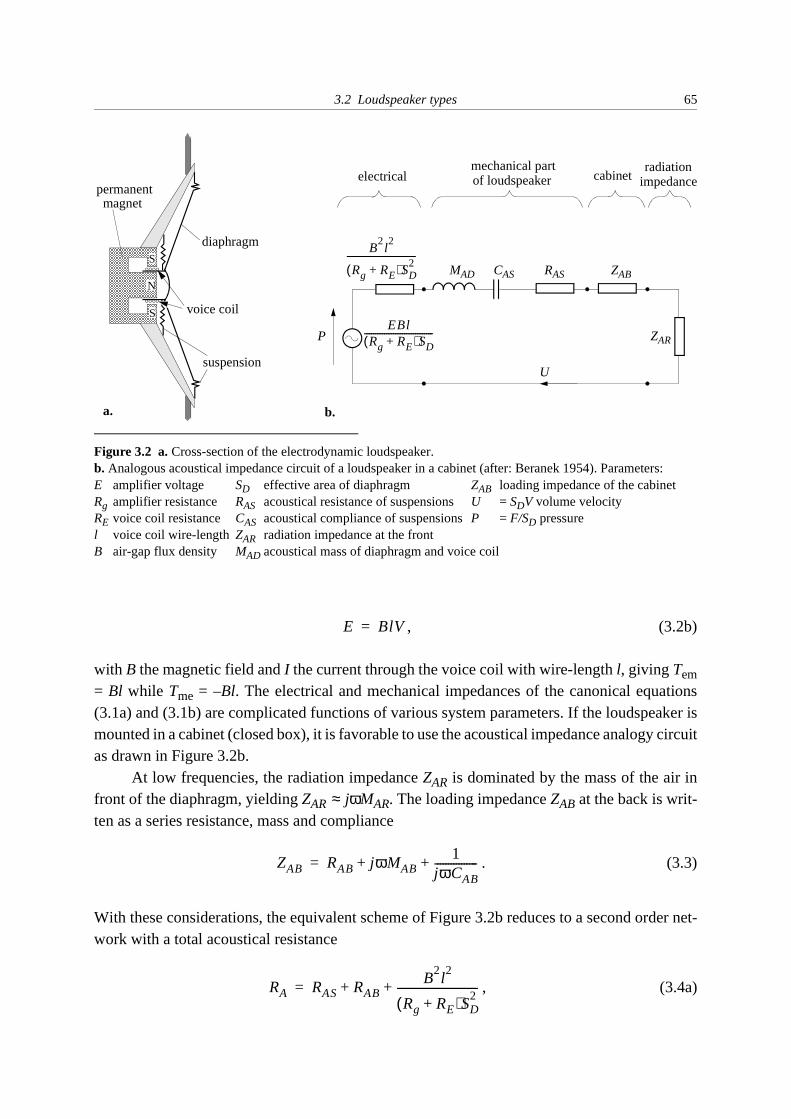
3.2 Loudspeaker types 65
, (3.2b)
with B the magnetic field and I the current through the voice coil with wire-length l, giving Tem= Bl while Tme = –Bl. The electrical and mechanical impedances of the canonical equations(3.1a) and (3.1b) are complicated functions of various system parameters. If the loudspeaker ismounted in a cabinet (closed box), it is favorable to use the acoustical impedance analogy circuitas drawn in Figure 3.2b.
At low frequencies, the radiation impedance ZAR is dominated by the mass of the air infront of the diaphragm, yielding ZAR jωMAR. The loading impedance ZAB at the back is writ-ten as a series resistance, mass and compliance
. (3.3)
With these considerations, the equivalent scheme of Figure 3.2b reduces to a second order net-work with a total acoustical resistance
, (3.4a)
E BlV=
S
S
N
suspension
voice coil
diaphragm
permanentmagnet
Figure 3.2 a. Cross-section of the electrodynamic loudspeaker. b. Analogous acoustical impedance circuit of a loudspeaker in a cabinet (after: Beranek 1954). Parameters:E amplifier voltage SD effective area of diaphragm ZAB loading impedance of the cabinetRg amplifier resistance RAS acoustical resistance of suspensionsU = SDV volume velocityRE voice coil resistance CAS acoustical compliance of suspensionsP = F/SD pressurel voice coil wire-lengthZAR radiation impedance at the frontB air-gap flux density MAD acoustical mass of diaphragm and voice coil
EBlRg RE+( )SD
-------------------------------
B2l2
Rg RE+( )SD2
-------------------------------MAD CAS RAS
ZAR
ZAB
U
P
electricalmechanical part of loudspeaker
radiationimpedancecabinet
b.a.
≈
ZAB RAB jωMAB1
jωCAB----------------+ +=
RA RAS RABB
2l2
Rg RE+( )SD2
------------------------------+ +=

66 Chapter 3: Loudspeaker Arrays
a total acoustical mass
, (3.4b)
and a total acoustical compliance
, (3.4c)
all connected in series. The resonance frequency of this system is given by
, (3.5)
with a quality factor
. (3.6)
Below resonance, the system is stiffness-controlled, i.e. the volume velocity U is proportionalto jωCA, while the system is mass-controlled above resonance (Beranek 1954):
. (3.7)
If the cabinet is small compared to the wavelength, the loudspeaker has monopole characteris-tics. Then, the free field sound pressure can be approximated by that of a volume velocity source
, (3.8)
or, with Equation (3.7),
. (3.9)
This expression shows that the sound pressure is proportional to the steering voltage for fre-quencies above resonance (which is the operational frequency range for normal loudspeakers).The frequency factor 1/jω of the volume velocity is fully compensated by the factor jω of theradiation impedance of the monopole.
If multiple electrodynamic loudspeakers are used to form a linear array for wave fieldsynthesis, the only frequency dependence that is left originates from driving function (2.30). Itstates that the input signals of the loudspeakers should be filtered by +3 dB/octave ( ). Inaddition, for a primary source behind the array a frequency-independent phase shift of +45º isnecessary, while it is – 45º for a source in front of the array.
MA MAD MAB MAR+ +=
CA
CASCAB
CAS CAB+--------------------------=
ω01
MACA
-------------------=
Q01
RA------
MA
CA-------=
U ω( ) E ω( )BljωMASD Rg RE+( )---------------------------------------------=
P r ω,( ) jωρ4π---------U ω( ) jkr–( )exp
r-------------------------=
P r ω,( ) ρE ω( )Bl4πMASD Rg RE+( )----------------------------------------------
jkr–( )expr
-------------------------=
k

3.2 Loudspeaker types 67
3.2.3 Electrostatic loudspeaker
The electrostatic loudspeaker consists of a conducting membrane and a perforated rigidplate, together forming a capacitor (Figure 3.3a). By applying an alternating voltage betweenthe plates, the membrane is forced to move to and fro. The steering voltage E is increased by atransformer and added to the polarizing voltage E0. Instead of one rigid plate, often two platesare used, one at either side of the membrane. The following relations also hold for this bal-anced (‘push-pull’) version, if the capacitance C0 is read as C0/2 (two capacitors C0 in series).The canonical equations for the electrostatic loudspeaker are given by (Hunt 1982)
(3.10a)
with E' = EN (N the ratio of turns of the transformer) and V the velocity of the membrane, and
, (3.10b)
conducting
h0
Figure 3.3 a. Electric circuitry for a single-sided electrostatic loudspeaker in its equilibrium state (with E = 0).The transformer TN brings the input signal voltages (~1 volt) in the range of 100 volt. A voltage source provides aconstant polarization voltage E0.b. Analogous electromechanical circuit of the electrostatic loudspeaker. Transformer TN has been removed fromthe circuit by incorporating the turns-ratio in the signal source voltage E' = NE. Transformer Tφ represents the trans-duction coupling between the electric circuit to the left and the mechanical analogy circuit to the right. The ratioof turns, φ = E0C0/h0, is calculated as the transduction coefficient Tem divided by the impedance in shunt position1/jωC0.The impedance ZM is due to the mechanical construction of the loudspeaker, while ZMR is the mechanicalradiation impedance. The negative capacitance –C0/φ2 is caused by electrostatic attraction between the membraneand the perforated plate (after: Hunt 1982).
I
C0E0E
perforatedplate membrane
1 : Na.
b.
I
ZMRE'
1 : φ
C0
ZM
F
V
TN
Tφ
–C0/φ2
blockingcapacitor
protective resistance
E′ IjωC0------------
E0V
jωh0-----------+=
FE0I
jωh0----------- ZMV+=

68 Chapter 3: Loudspeaker Arrays
where ZM is the mechanical impedance of the loudspeaker construction. These equations showthat the transduction coefficient is symmetrical: Tem = Tme = E0/jωh0. The corresponding elec-tromechanical analogy circuit is drawn in Figure 3.3b. With the aid of this scheme, it is foundthat
, (3.11)
in which φ = E0C0/h0 and the mechanical radiation impedance is defined by ZMR = F/V. If thedenominator of (3.11) is close to unity, a more or less frequency-independent relation resultsbetween the voltage E' and the force F. In that case,
. (3.12)
At low frequencies, the electrostatic loudspeaker acts more or less as a dipole. The far-fieldsound pressure for such a source can be calculated from the sound pressure of two monopolesources with volume velocities +U and –U at a small distance ∆r from each other, giving
, (3.13)
with ϕ the angle between the point of observation and the line connecting the imaginary mono-poles. Since, according to Newton’s second law, the dipole’s force acting on the surroundingmedium, is given by
, (3.14)
the sound pressure can be evaluated by combining (3.12), (3.13) and (3.14):
. (3.15)
The frequency response in the far-field increases with 6 dB per octave, because of the factor jk.Since in normal use, e.g. for stereophonic reproduction, a flat frequency response is desired, theelectrostatic loudspeaker is usually furnished with an internal filter of –6 dB per octave (and afrequency indepedent phase shift of –90º). Instead, if the electrostatic loudspeaker is used forwave field synthesis, an internal filter of –3 dB per octave (1/ ) is needed, as can be seen fromdriving function (2.31). The filter should have a phase shift of for a source behind the arrayand for a source in front of the array.
Fφ
1 φ2jωC0ZMR( ) ZM ZMR⁄+⁄–
---------------------------------------------------------------------------E′=
F ω( )E0C0N
h0-----------------E ω( )=
P r ω,( ) jωρU ω( )∆r4π------------------------------ jk ϕ jkr–( )exp
r-------------------------cos=
F ω( ) jωρU ω( )∆r=
P r ω,( )E0C0N
4πh0-----------------E ω( )jk ϕ jkr–( )exp
r-------------------------cos=
k45°–
135°–

3.3 Directivity 69
3.3 Directivity
In Section 2.5.2 it has been shown that controlling directivity is of great importance inwave field synthesis, because it allows proper control of spatial aliasing. The directivity oftransducers can be either frequency-independent or frequency-dependent. For instance, the(ideal) dipole has frequency-independent directivity, because of the factor cos(ϕ) being inde-pendent of frequency. Since the effect of spatial aliasing depends on frequency and direction, itis obvious to use array elements with frequency-dependent directivity in order to control spa-tial aliasing.
Frequency-dependent directivity is caused by different parts of the radiating (or receiv-ing) diaphragm having different distances to the point of observation (or emission), see Figure3.4. At low frequencies, where the dimensions of the diaphragm are small compared to thewavelength, the transducer essentially behaves either as an ideal monopole or as an idealdipole, according to its mechanical construction. At higher frequencies the shape and excur-sion of the diaphragm must be taken into account.
Apart from the directivity of a single transducer, an array of transducers can also gener-ate a directivity pattern, since an array may be considered as one large, but discretized dia-phragm. In this section it will be shown that, through relating directivity to spatial convolution,a thorough understanding and control of directivity is possible.
λ
pathlengthdifference
diaphragm
diaphragm
½λ½λ
2½λ
3λ
b.a.
Figure 3.4 Frequency-dependent directivity. a. If the width of the diaphragm is small compared to the wavelength,the maximum pathlength difference will be likewise and directivity is negligible. b. If the width of the diaphragmis large compared to the wavelength, destructive interference occurs in certain directions if the waves originatingfrom different parts of the diaphragm have opposite phases.

70 Chapter 3: Loudspeaker Arrays
3.3.1 Spatial Fourier transform and directivity
The directional behavior of loudspeakers* is usually studied by considering directivitypatterns for several frequencies. If the diaphragm is moving coherently, the directivity patternsfor all frequencies can be calculated from the typical directivity function for that shape of dia-phragm. For example, the far-field sound pressure of a rigid circular piston, mounted in an infi-nite baffle, is given by (Beranek 1954)
, (3.16a)
where ϕ is the radiation angle and L the directivity function
, (3.16b)
with J1 the first order Bessel function of the first kind. Apart from the factor L, the sound pres-sure (3.16a) is twice that of a monopole volume velocity source (3.8) in a free field, due to theinfinite baffle. For this source the directivity function and a few directivity patterns are drawnin Figure 3.5.
Electrodynamic loudspeakers behave as rigid pistons in the low and mid frequencyrange. Above some frequency, usually a few kHz, they exhibit cone break-up effects, i.e. fre-quency-dependent modes of bending waves occur over the diaphragm. This is a result of theconstruction: the driving force from the voice coil is not uniformly spread across the radiatingsurface. Because of this property, the directivity characteristics of electrodynamic loudspeak-ers are difficult to model, and hence to control. Electrostatic diaphragms generally do not suf-fer from break-up effects because the electrostatic force is almost homogeneous across thesurface of the membrane. Therefore, electrostatic loudspeakers are well-suited for designingdirectivity characteristics. In the following, the directivity function of an arbitrarily shaped(electrostatic) dipole diaphragm will be derived.
For a dipole source distribution across a surface A within the xy-plane, the Rayleigh IIintegral can be used to calculate the sound pressure in a point R far away from that surface
, (3.17)
where P(ω) is the sound pressure at the surface A, and ϕ is the angle with the z-axis. In general,the surface of integration of Rayleigh II consists of the whole xy-plane, but since P(ω) is zerooutside A the integration is confined to A only.
* For convenience the theory is illustrated for loudspeakers only, but because of reciprocity the results alsoapply to microphones.
PjωρU
2π--------------L ka sinϕ( ) jkr–( )expr
-------------------------=
L ka sinϕ( )2J1 ka sinϕ( )
ka sinϕ--------------------------------=
PR1
2π------ P ω( )1 jkr+
r2
---------------- ϕ jkr–( )expcos xd ydA∫=

3.3 Directivity 71
Figure 3.5 Directivity function and patterns for a rigid circular piston.
diaphragm
a. x
r0
R
ψ0
Figure 3.6 a. Fraunhofer approximation for radiating diaphragm. The vector r from a point at the diaphragm to Rcan be expressed in terms of r0 (pointing from the center of the diaphragm to R), the angles ϕ0 and ψ0, and coor-dinates x and y, as given by (3.18). b. Projections on the x- and y-axis yields the strength distributions lx and ly.
z
ly(y)
lx(x)
y
x
diaphragm
b.
y
ϕ0 r

72 Chapter 3: Loudspeaker Arrays
In the Fraunhofer area, where r » d2/λmin with d the diameter of the diaphragm, the fol-lowing approximation is valid (Berkhout 1987)
, (3.18)
where r0 is the distance from the center of the diaphragm to receiver position R, see Figure 3.6a.Since kx = k sinϕ0 cosψ0 and ky = k sinϕ0 sinψ0, the sound pressure at R can be written as
. (3.19)
The surface integral can be factorized by realizing that the driving force of a small (vertical) col-umn of the surface of the diaphragm, for which kx is constant, can be assigned to a point sourceat the x-axis, yielding a strength function lx(x) for a line distribution along the x-axis, see Figure3.6b. An analogous procedure can be used for the y-direction. Integral (3.19) then changes into
, (3.20)
in which F(ω) = 2AP(ω) is the force of the diaphragm acting on the air. The strength functionslx(x) and ly(y) are normalized: and . With spatial Fourier trans-forms Lx(kx) and Ly(ky) defined as
(3.21a)
and
, (3.21b)
the sound pressure at R evaluates to
, (3.22)
in which the subscript ‘0’ has been omitted. Notice that this expression reduces to (3.13), withsubstitution of (3.14), if k approaches zero, i.e. for low frequencies where and
. This equation states that the sound pressure in the far-field is proportional to thespatial Fourier transforms of the diaphragm’s strength functions in x- and y-direction. It therebyprovides a clear method to design directivity characteristics for well-behaving electrostaticloudspeakers. In the next paragraph, an ideally shaped array loudspeaker is designed.
r r 0 x ϕ0 ψ0 y ϕ0 ψ0sinsin–cossin–≈
PR jk ϕ0
jkr0–( )exp
2πr0---------------------------cos P ω( )e
jkxxe
jkyyxd yd
A∫=
PR jk ϕ0
jkr0–( )exp
4πr0---------------------------cos F ω( ) lx x( )e
jkxxx ly y( )e
jkyyyd∫d∫=
lx x( ) xd∫ 1= ly y( ) yd∫ 1=
Lx kx( ) lx x( )ejkxx
xd∞–
∞
∫=
Ly ky( ) ly y( )ejkyy
yd∞–
∞
∫=
PR Lx kx( )Ly ky( )F ω( )4π
------------ jk ϕ jkr–( )expr
-------------------------cos=
Lx kx( ) 1≈Ly ky( ) 1≈

3.3 Directivity 73
3.3.2 Spatial low-pass filter by diaphragm shaping
The requirements for a spatial reconstruction filter for loudspeaker arrays have been dis-cussed in Section 2.5.2. It has been shown there that a low-pass kx-filter is needed as a recon-struction filter. The spatial cut-off frequency is determined by the spatial Nyquist frequencykx,Nyq = π/∆x, where ∆x is the spacing between the array elements. Theoretically a block-filterin the kx-domain would be ideal, but because of the Fourier coupling (3.22) this would requirea sinc-filter (sin(x)/x) in the x-domain. Such a filter consists of many side lobes, i.e. side dia-phragms alternating in phase and anti-phase. The feasibility of such an ideal filter is studied inthe next paragraph. In this paragraph a simple and practical design is given, based on a singlediaphragm with an optimized shape.
As a first trial, a rectangular diaphragm is taken, see Figure 3.7. The discretization of thedriving functions for wave field synthesis in the xz-plane (Section 2.5) did not impose anyrequirements for the vertical directivity ( ky-filter). Therefore the designer is free to fulfill otherdemands. If it is desirable that ceiling and floor reflections are avoided, the width of the dia-phragm in the y-direction should be large. If, however, part of the audience is sitting close tothe arrays (viewing the array under a large vertical angle), vertical directionality should besmall to obtain a frequency-independent response for the whole audience area. In that case, thewidth in the y-direction should be small. If only the x-direction is considered, the frequency-dependent part of the directivity function is given by the Fourier transform of a block-functionwith width 2a:
. (3.23)
If the loudspeakers are mounted tightly, the spacing between the centers of two adjacent dia-phragms equals the width ∆x = 2a. The attenuation of this kx-filter at the Nyquist frequency istherefore Lblock(kx,Nyq) = 2/π, giving a level of only –3.9 dB with respect to the main lobe. Thefilter has side lobes of –13 dB at kx = ± 1.43π/a.
front view
diaphragm
xy
ly
y
Ly (dB)
ky
–13 dB
lx
x
Lx (dB)
kx
–13 dB
Figure 3.7 Directivity functions for a rectangularly shaped diaphragm. The width of the block-function is inverse-ly proportional to the width of its Fourier transform, a sinc-function.
Lblock kx( )kxa( )sin
kxa---------------------=

74 Chapter 3: Loudspeaker Arrays
The performance of the filter can be improved by smoothening the edges, but withoutincreasing the spacing between adjacent array elements. This is realized by a rhombic dia-phragm as shown in Figure 3.8a. Its strength function lromb(x) is trapezoidal: it is a convolutionof two block functions with widths 2a1 and 2a2 respectively, a1 > a2 . Therefore the directivityfunction is the product of two sinc functions:
(3.24a)
with
(3.24b)
and
. (3.24c)
The performance of this filter can be optimized with certain constraints. The optimization taskwill be to find the ratio a1/a2 for which side lobes are reduced maximally while maintaining areasonable response within the pass-band |kx| < kx,Nyq. It will be advantageous to choose a ratio
Figure 3.8 a. Construction of a rhombic diaphragm. b. kx-filter for ratio of widths a1/a2 = 1.43.
original block
rhomboid
lromb(x) = l1(x)* l2(x)
l2(x)
l1(x)
2a2
2a1
a.
b.
trapezoidalstrength function
Lromb kx( ) L1 kx( )L2 kx( )=
L1 kx( ) kxa1( )sin kxa1( )⁄=
L2 kx( ) kxa2( )sin kxa2( )⁄=

3.3 Directivity 75
a1/a2 in such a way that the first side lobe of L1 is canceled by the first zero of L2, see Figure3.8b. Because L1 has its first side lobe at kx = ±1.43π/a1, while L2 has its first zero at kx= ±π/a2,it is clear that a1/a2 = 1.43 meets the requirement.
For any ratio, two possible rhombic diaphragms can be chosen: ∆x = 2a1 or ∆x = 2a2.The choice does not affect the level of the side lobes, but defines the position of the spatialNyquist frequency with respect to the filter shape. In Figure 3.9 both settings are compared.The narrow filter of Figure 3.9b gives the best rejection in the stop-band (where |kx| > kx,Nyq),but it also affects the pass-band considerably (–13 dB at kx,Nyq). The following paragraphdescribes how a better fit can be achieved by applying a discrete kx-filter to the driving signals.
3.3.3 Spatial low-pass filter by discrete spatial convolution
Consider an array of identical elements, each with strength function l(x). Now, instead ofdriving only one element with some driving function Q(x, ω), a series of 2N+1 elements isdriven by the same signal but at different gain. This results in a total strength function
, (3.25)
where cn is the weight of the nth array element, and ∆x the spacing between the elements. Thetotal strength function can be written as a sum
. (3.26)
The Fourier transform of this sum,
Figure 3.9 Spatial Nyquist frequency for a kx-filter with a1/a2 = 1.43.
lN x( ) c N– l x N∆x+( ) c N 1–( )– l x N 1–( )∆x+( ) …+ +=
c 1– l x ∆x+( ) c0l x( ) c1l x ∆– x( ) … cN 1– l x N 1–( )– ∆x( ) cNl x N– ∆x( )+ + + + +
lN x( ) cnl x n– ∆x( )n N–=
N
∑=

76 Chapter 3: Loudspeaker Arrays
, (3.27)
can be evaluated by interchanging summation and integration and calculating the Fourier trans-form of the elements
. (3.28)
where L(kx) is the Fourier transform of the strength function l(x) of a single element. Therefore,(3.27) reads
, (3.29)
or, for symmetrical weights cn= c–n,
, (3.30a)
with
. (3.30b)
This directivity function is the product of a continuous part L(kx) and a periodic part CN(kx) withperiod 2π/∆x. In the space domain, the resultant strength function lN(x) can be written as a con-volution of a continuous strength function l(x) with a pulse sequence, see Figure 3.10.
Therefore, it is possible to reshape the directivity function of a single element by opti-mizing the weights of neighboring array elements. Of course, there is a restriction because ofthe periodicity of the Fourier transform of the discrete pulse sequence. Furthermore, the far-field conditions should be satisfied, which means that only a small number of array elementsmay be involved in the spatial convolution.
Two examples demonstrate the influence of a discrete spatial convolution filter with N =2 (five array elements). Figure 3.11 shows the optimization result for a flat pass-band, i.e. for|kx| < kx,Nyq. The spacing between the rhombic elements is ∆x = 2a1 (with a1/a2 = 1.43). Theresultant kx-filter (thick line) is a composition of the rhomboid’s kx-filter (Figure 3.9a) and thespatial convolution filter applied to the array elements. Only a slight change (2 to 3 dB) in theresponse is necessary to obtain a nearly flat pass-band. Note that, due to the periodicity of CN,it is impossible to reduce the response in the stop-band without attenuating the response in thepass-band. The reason for this is that the spatial convolution filter is sampled at the same inter-val ∆x as the synthesis operator. Therefore the same Nyquist condition is valid for both dis-cretized functions of x.
LN kx( ) cnl x n– ∆x( )ejkxx
n N–=
N
∑ xd∞–
∞
∫=
cn∞–
∞
∫ l x n– ∆x( )ejkxx
dx cn∞–
∞
∫ l x'( )ejkx x' n∆x+( )
dx'=
cnejkxn∆x
L kx( )=
LN kx( ) L kx( ) cnejkxn∆x
n N–=
N
∑=
LN kx( ) L kx( )CN kx( )=
CN kx( ) c0 2 cn kxn∆x( )cosn 1=
N
∑+=

3.3 Directivity 77
c0
c2
c1c-1
c-2
l(x)
lN(x) = cN(x)* l(x) LN(kx) = CN(kx) L(kx)
L(kx)
cN(x)
CN(kx)
Figure 3.10 Strength function lN(x) can be constructed by spatial convolution of the strength function l(x) of asingle array element with the spatial pulse sequence cN(x). The coefficients cn are equal to the gain of the arrayelements at location n∆x.
0
0
x-domain kx-domain
x
x
x
kx
kx
kx
Figure 3.11 Optimization of the pass-band response for the rhomboids with ∆x = 2a1. The resultant kx-filter LN isthe product of the directivity function Lromb of a single rhombic element and the spatial Fourier transform CN forweighting coefficients: c0, c1 ,c2= 1, –0.11, 0.02.

78 Chapter 3: Loudspeaker Arrays
For an optimum stop-band attenuation, the rhomboids with ∆x = 2a2 should be taken, seeFigure 3.12. The kx-filter of this rhomboid is already down –13 dB at the spatial Nyquist fre-quency, and can be further reduced to less than –20 dB in the whole stop-band. This isachieved by a positive weight at the nearest neighbor and a negative weight at the next neigh-bor element. Such a configuration of weights produces a wider, but more gently tapered centraldiaphragm, without increasing the sample interval ∆x.
3.4 Design of arrays for audio reproduction
In designing a loudspeaker array for audio reproduction, both the spatial and temporalproperties of the loudspeaker elements need to be considered. As for the spatial properties, acontrolled directional behavior is required, if little spatial aliasing is permitted. The temporalconditions can be summarized by stating that the sound quality of the loudspeaker elementshould be satisfactory within a large frequency range. This condition is formulated here in asubjective manner, and involves a large number of physical properties like distortion, soundpower, frequency response and efficiency. High quality loudspeakers for conventional repro-duction will generally be applicable for audio reproduction by wave field synthesis as well, butthere are some different needs because of the special nature of arrays. In conventional electro-dynamic loudspeaker systems, the audio bandwidth is usually covered by two or three driverswith complementary frequency ranges, because it is virtually impossible to construct a singledriver covering the whole audio spectrum with enough sound power. Since the sound power inan array system is generated by more than one element, the sound power criterion is moderated
Figure 3.12 Optimization of the stop-band for the rhomboids with ∆x = 2a2. The attenuation for |kx| > kx,Nyq isgreater than 20 dB. The resultant kx-filter LN is the product of the directivity function Lromb of a single rhombicelement and the spatial Fourier transform CN for weighting coefficients: c0, c1 ,c2= 1, 0.17, –0.12.
kx,Nyq
3.4 Design of arrays for audio reproduction 79
considerably. Only if the virtual source is exactly at the position of an array loudspeaker, allpower has to be generated by one driver. By excluding the vicinity of the array from the virtualsource area, the power problem can be solved adequately. Practically, at least two or threearray elements bear the burden of sound power generation, if a strip of width ∆x parallel to thearray is excluded from presence of virtual sources. Therefore, small low-power array elementswith large frequency ranges can be used in array systems.
If higher sound power is required, two-way or three-way arrays can be constructed.These arrays consist of two or three different drivers that are active in different sub-bands. Theupper bound of the bandwidth determines the maximum spacing ∆x for that specific sub-bandloudspeaker. For example, a two-way array system with crossover frequency fx requires aspacing between the woofers of ∆xwoofer = c/2fx maximally.
Two types of (one-way) loudspeaker arrays are investigated in this section: first, an elec-trodynamic array with (nearly) full range low-power drivers, and second, an electrostatic arraywith controlled directivity elements. After a description and qualification of both types ofloudspeaker arrays, measurements on the synthesized wave fields are presented. Finally it isconsidered which one of both types of arrays is more suitable for integration in a wave fieldsynthesis system for sound reproduction.
3.4.1 Electrodynamic array
Directivity
Because of nodal cone resonances, the directivity characteristics of an electrodynamicloudspeaker are difficult to control. Nevertheless, the directivity pattern of a rigid piston is areasonable approximation in the low and mid frequency range. Most commercially availableelectrodynamic loudspeakers have circular diaphragms with equal directivity in the verticaland horizontal plane. If the horizontal directivity is desired to differ from the vertical directiv-ity, an oval shaped diaphragm is eligible, with the wider dimension aligned in the direction ofthe highest directivity.
The directivity function of an oval diaphragm is shown in Figure 3.13, together withthose of a circle and a rhomboid. Here, the wider dimension of the oval lies in the horizontalplane, which improves the directional behavior in that plane. For each of the three shapes, thedirectivity in the vertical plane is kept within bounds by restricting the dimensions in thatdirection. The directivity of the oval piston is higher than that of the circular piston, but lowerthan that of the rhomboid. The dimensions of the oval diaphragm correspond to those of theloudspeaker shown in Figure 3.14, which is a candidate for the construction of an electrody-namic array.
Three polar patterns of that loudspeaker are shown in Figure 3.15. The measured direc-tivity patterns for 4 kHz and 16 kHz show that the directivity of the loudspeaker lags behindthat of the rigid piston model, which must be a result of irregular diaphragm motion. Theasymmetrical shape for the highest frequency is presumably caused by the attachment of thevoice coil wires at one side of the diaphragm.

80 Chapter 3: Loudspeaker Arrays
Figure 3.13 Comparison between the directivity functions of a circular, an oval and a rhombic diaphragm. Theoval consists of two semicircles, each with radius 0.22 ∆x, and a rectangle of width 0.56 ∆x, where ∆x is the dis-tance between nearly touching adjacent diaphragms. The radius of the circular diaphragm is 0.22 ∆x; the rhombicdiaphragm has a ratio a1/a2 = 1.43, where ∆x = 2a1.
Figure 3.14 Electrodynamic loudspeaker with oval shaped diaphragm (Philips ID 25952/X8). Shown measuresare in centimeters.
2.411.0
12.7
5.8
Figure 3.15 Measured (thick) and theoretical (thin) polar patterns for the oval electrodynamic loudspeaker.

3.4 Design of arrays for audio reproduction 81
From these directivity measurements it is obvious that this type of loudspeaker is notspecially equipped for reducing spatial aliasing in the synthesized wave field. However,because of its very reasonable sound quality (tested by concentrated listening), wide frequencyrange (140 Hz – 20 kHz), low weight, small vertical size and low costs, it was decided to usethese drivers in building an electrodynamic array. The design of this array is based on the fol-lowing considerations concerning the volume of the enclosure in which the loudspeakers aremounted.
Enclosure volume
The loudspeakers can be placed either in separate cabinets or in one large hollow bar. Ifthe latter option is chosen, acoustic coupling from within the bar can be avoided by partitions,creating separate enclosures. The volume (per element) determines the resonance frequency ω0and quality factor Q0. The measured values for this type of loudspeaker in a large baffle are ω0= 2π·134 rad/s and Q0 =1.4 rad m/Ω, respectively. If the loudspeaker is mounted in an enclo-sure, both the resonance frequency and the quality factor will be higher, since the complianceof the enclosed air, given by (Beranek 1954)
, (3.31)
where VB is the volume of the enclosure, κ 1.4 for adiabatic compression of air, and p0 105
N/m2, lowers the total acoustical compliance CA that appears in the denominator of (3.5) and(3.6). Therefore VB should be large to keep ω0 and Q0 low. However, a large cabinet volumeraises the dimensions (and weight) of the array, so that a compromise must be made in choosingthe size of the cabinet. A practical volume will be that for which CAB approximately equals CAS,so that both compliances contribute equally to the total compliance. With CAS = 1.3·10-8 m5/Nfor this driver, a volume of about 1.8 dm3 is calculated. Figure 3.16 plots the measured frequen-
CAB
VB
κp0---------=
≈ ≈
Figure 3.16 Frequency response near the resonance frequency of the loudspeaker of Figure 3.14, as a function ofthe enclosure volume: 2.0 dm3 (thick solid); 1.7 dm3 (dashed); 1.4 dm3 (thin solid).

82 Chapter 3: Loudspeaker Arrays
cy response as a function of the loudspeaker enclosure volume. As the volume increases, theresonance peak is damped more, while the top position shifts towards lower frequencies. Fromthese results it appears reasonable to keep the volume in the 1.7 – 2.0 dm3 range.
Loudspeaker spacing
The spacing between the loudspeakers determines the value of the spatial aliasing fre-quency. From experience with synthesis arrays for sound enhancement, it is known that analiasing frequency of at least 1500 Hz is favorable for correct sound localization (i.e. Vogel1993 and Start 1997). This is not surprising: if the wave fronts are reconstructed correctlybelow 1500 Hz, then the interaural time differences, which dominate localization (Wightmanet al. 1992), will correspond to those heard for the original wave fronts. If the aliasing fre-quency is decreased (by increasing ∆x), the localization accuracy decreases as well. Further-more, in informal listening tests it was noticed that the apparent width of the image increaseswith increasing spacing between the loudspeakers. This can be understood by realizing thataliased waves, which travel in wrong directions, interfere with the correct waves, thereby caus-ing phase distortion between the ear signals, and hence will degenerate interaural correlation.Potter (1993) showed that the perceived image of a true source broadens with decreasing inter-aural correlation for frequencies below 1600 Hz. Therefore, the aliasing frequency of an audioreproduction system based on wave field synthesis should not drop far below 1600 Hz. Thiscondition preserves spaciousness for virtual sources, one of the requirements mentioned inSection 1.5.
∆x = 12.7
acoustically transparent cloth
railsdriver
multiplex
cross-section
front view
leads canal
Figure 3.17 Cross section and front view of the 16-channel electrodynamic arraybar. Dimensions of the bar: l×b×h= 203×27×9 cm. Weight: 21 kg. Power handling of single loudspeaker: 3 W rms, giving 90 dB SPL at 1 m.
1.8 dm3

3.4 Design of arrays for audio reproduction 83
Based on these considerations, a 16 channel electrodynamic array was built with anenclosure volume of about 1.8 dm3 per array element, and a loudspeaker spacing of 12.7 cm,which is the minimum spacing between these loudspeakers, see Figure 3.17. This results in aspatial aliasing frequency of 1340 Hz.
3.4.2 Electrostatic array
Because of the promising directivity characteristics, also an electrostatic array-strip withrhombic elements was built. It consists of 16 elements with a spacing ∆x = 11 cm (with falias =1545 Hz), see Figure 3.18. The rhombic elements have an approximate ratio a1/a2 = 1.43. Thewidth in the vertical direction is kept small, 7 cm, to avoid strong directionality in that direc-tion: listeners will not notice strong spectral changes when standing up or sitting down. Thewidth of the elements is set to 2a1 as in Figure 3.9a* .
The kx-filter response can be calculated directly from the directivity patterns via the rela-tion kx = 2πf sin(ϕ)/c. From a theoretical point of view, the measured polar pattern for any fre-quency may serve as data in calculating the element’s kx-filter, provided that the measuredpolar patterns are consistent†. Figure 3.19 proves that there is good agreement between the
* An electrostatic array with the other setting, ∆x = 2a2, is difficult to construct on condition that its y-direc-
tionality be small. It would consist of very narrow and fragile elements.† Polar patterns are mapped to part of the kx-filter: the polar pattern for f Hz is mapped between kx = –2πf/c
and +2πf/c. High frequency polar patterns thus provide more information of the kx-filter than low frequency
patterns. In theory, all mapped polar patterns fit the kx-filter response exactly.
11 cm
7 cm
7 cm
10 cm
1.7 kV
47 µF
12 Ω
25 : 3000
Figure 3.18 Front view and electric circuit of the prototype electrostatic loudspeaker array. The RC-filter at thetransformer input has a low frequency cut off at 280 Hz. The grounded perforated plate as well as the membraneare made of one piece; 16 separate plates are used as (hot) signal electrodes. The total thickness of the array-stripis 0.5 cm.
10 ΜΩ

84 Chapter 3: Loudspeaker Arrays
measured and calculated directivity characteristics. It is therefore allowed to estimate the kx-filter of an element from the measured polar data for only one high frequency component, seeFigure 3.20. The filter bears reasonable comparison with the predicted response. The shape ofthe main lobe is very close to the theoretical shape, except near kx = 70 m-1 where a side lobe‘joins’ the main lobe. Though the level of the side lobes is higher than predicted, the positionof the lobes is as expected. The measurements indicate that the directivity characteristics ofsimple electrostatic loudspeakers can indeed be controlled reasonably well.
A disadvantage of the high directionality of the rhombic array elements is that the virtualsources must be confined to areas with a limited angle of incidence towards the audience.Otherwise, the reduction of the bandwidth becomes audible. A solution for this side effect ofkx-filtering is the use of curved arrays, see Figure 3.21. The angle of incidence ϕ at the array, asseen from a listener looking in the direction of the virtual source, determines the perceivedbandwidth of that source. If the angle is small, the bandwidth is large and vice versa. The lis-tening area with full bandwidth is therefore small for virtual sources to the side. If the corner is‘rounded’, a much larger listening area is created.
Figure 3.19 Measured (thick) and theoretical (thin) polar patterns for one element of the electrostatic array.

3.4 Design of arrays for audio reproduction 85
3.4.3 Comparative measurements
The frequency response of one element of both the electrostatic and electrodynamicarray are measured in an anechoic room, see Figure 3.22. This figure clearly shows the differ-ent frequency dependence of electrostatic and electrodynamic loudspeakers. From (3.9) it fol-lows that a flat frequency response is globally expected for an electrodynamic loudspeaker,while according to (3.15) a slope of 6 dB per octave is found for an electrostatic loudspeaker.This is confirmed by the measurements.
Figure 3.20 Comparison between the kx-filter of a rhombic element as calculated from measured polar data (f =12.5 kHz), and the theoretical rhombic response (thin line).
Figure 3.21 a. If the arrays consist of highly directional loudspeakers, only a part of the audience area is radiatedin full bandwidth. Here the coverage area for incident angles ϕ of less than 45º is drawn for a source near the cornerof an L-shaped array. b. If the corner is canted, a much larger area of coverage is achieved.
audience
a. b.
arrays arrays
ϕ
|ϕ|<45º|ϕ|<45º
ϕ
virtual sourcevirtual source
audience

86 Chapter 3: Loudspeaker Arrays
Because of the small membrane area (70 cm2), the sensitivity of the electrostatic elementis quite low. Especially the poor bass response can be problematic, because bass equalizationwill cause audible distortion if the membrane exceeds the linear excursion region. Enlargementof the surface area of the membrane will enhance the bass response, but will also affect thealiasing frequency and/or the directivity in the vertical plane, in an indirect manner. An addi-tional array of (electrodynamic) low-frequency loudspeakers is probably a better solution,however at the expense of a more complicated construction and higher costs.
It should also be mentioned that the sound quality of music produced by the prototypeelectrostatic array was suffering from irregular sputtering, probably caused by leakage of thepolarization charge. A second prototype with a more robust construction exhibited less sputter-ing, but also had lower sensitivity due to a larger gap between the electrodes. Nevertheless, the(first) prototype was sufficiently stable to explore its behavior in a series of plane wave synthe-sis measurements.
Figure 3.23 plots a set of measured impulse responses of a plane wave parallel to thearrays. At t = 0.7 ms the main wave front arrives at the microphone array. While the electro-static array reconstructs the plane wave remarkably well, the response of the electrodynamicarray shows an aliasing tail. In a single impulse response taken from this data set, see Figure3.24a, this is visible as a sequence of separate pulses for the electrodynamic array, while theeffect is much weaker for the electrostatic array. This can be understood as follows: the loud-speakers at the right end of the electrodynamic array still radiate much high frequency energyin the direction of the microphone at x = –0.45, so the contribution of each loudspeaker is visi-ble as a separate pulse in the total response. In the frequency domain (Figure 3.24b), the pulsetrain causes a comb filter spectrum. The dips of the electrostatic response are less pronouncedthan those of the electrodynamic response.
Figure 3.22 On-axis sound pressure level of one electrostatic rhombic loudspeaker (thick) and one electrodynamicoval loudspeaker (thin), driven at the same input voltage level.

3.4 Design of arrays for audio reproduction 87
Whether these effects of spatial aliasing are audible depends on external circumstanceslike the type of source signal and the listening environment. In a static situation, i.e. motionlesslistener and source, the aliased wavelets are perceived as a subtle broadening of the virtualsource, rather than as coloration. If the listener or the virtual source moves, the comb filter dipswill shift gradually, which can be understood from Figure 3.23b where the intervals betweenaliased wavelets increase as the receiver moves away from the center. These spectral changesare clearly audible in an anechoic room, but tend to drown in the reflections of a normal listen-
Figure 3.23 a. Measured xt-diagram of a plane wave synthesized by the electrostatic array in an anechoic room.The measurement microphone is moved stepwise along a line parallel to the array. The impulse responses are con-volved in the time-domain with a Gaussian wavelet. The cut-off frequency of the Gaussian wavelet is 3.1 kHz,which is twice the Nyquist frequency (2.35) for ∆x = 11 cm. (Distance of measurement line: 2 m; angle of incidenceof the plane wave: 0º; array from x = –0.9 to +0.9 m)b. Measured xt-diagram of a plane wave synthesized by the electrodynamic array. The cut-off frequency of theGaussian wavelet is 2.7 kHz, which is twice the Nyquist frequency for ∆x = 12.7 cm. Clearly the effects of spatialaliasing are visible as wavelets after the actual wave front. (Array from x = –1.0 to +1.0 m)
a. b.
Figure 3.24 a. Impulse responses of the electrostatic and electrodynamic array, reproducing a plane wave. Takenfrom the xt-diagrams of Figure 3.23 at the position of the arrow. b. Spectra of these impulse responses (arb. offset).
b.a.

88 Chapter 3: Loudspeaker Arrays
ing room. Start (1997) also observed that the coloration (of the virtual source) introduced by awave field synthesis system for direct sound reinforcement, can be neglected in comparisonwith the coloration caused by the reflections of a concert-hall.
In this context it should be mentioned that a conventional stereophonic recording suffersfrom severe coloration during reproduction on two loudspeakers in an anechoic room. Espe-cially if the listener moves off the central axis, a tonal sweep is clearly heard. This effect isexplained by Figure 1.16, where a different pattern of comb filter dips is produced at differentreceiver positions. In a normal listening environment however, it is difficult to distinguishbetween the sound color of a phantom source in the midst of two loudspeakers and a truesource at that position. Seen in this light, the spectral irregularities introduced by a wave fieldsynthesis array with low directivity seem much less dramatic.
Eventually, because of its good sound quality, reliability and wide bandwidth, the elec-trodynamic array has been selected for the laboratory demonstration system. If the efficiencyof the electrostatic array can be enhanced, e.g. by optimizing the construction of the electrodes,the application of these arrays will become feasible too.
3.5 Conclusions
In this chapter, the general properties of electrodynamic and electrostatic loudspeakershave been investigated, as well as their applicability for wave field synthesis. It is found thatthe driving signals for electrodynamic arrays need a filtering of +3 dB per octave, while for theelectrostatic arrays –3 dB per octave is needed, besides an additional phase factor dependingon the position of the virtual source.
Since effects of spatial aliasing in the synthesized wave field depend on both the radia-tion angle and on frequency, a clear understanding of the directional behavior of transducers isof great importance. It is shown how the shape of the diaphragm of a transducer can be charac-terized by a directivity function, which in its turn defines the kx-filter that is a tool for reductionof spatial aliasing. The optimization of the shape of the kx-filter is described in terms of spatialconvolution filters, which allows for a generalization of the concept of directivity from a singlearray element (with an optimally shaped diaphragm) towards subarrays (with optimizedweighting coefficients).
An electrodynamic as well as an electrostatic array have been designed and tested. Theelectrodynamic array consists of small drivers with fairly good sound quality in a wide fre-quency range, but without controllable directivity characteristics. Measurements on the elec-trostatic array with diaphragms of optimized shape prove that spatial aliasing can be reducedconsiderably compared to the electrodynamic array. However, the bass response and the over-all sound quality of the electrostatic loudspeakers are still insufficient. Therefore, the electro-dynamic array is selected for use in the laboratory wave field synthesis system.

89
Chapter 4
Concept and Implementation of
WFS Reproduction
4.1 Introduction
The concept of sound reproduction, as developed in this chapter, is based on the theoryof wave field synthesis (WFS) that goes back to the Kirchhoff-Helmholtz integral expression.Several successive simplifications and approximations of this expression are necessary to con-struct a realizable concept. The final formulation is held generic to allow the implementationof a wide range of reproduction systems that differ in flexibility, quality and dimensions.
The reproduction concept comprises three phases: recording, storage and/or transmis-sion, and playback (Section 4.2). The recording method is similar to existing multi-channelrecording techniques, but an impulse is given towards the development and integration of sur-round sound microphone techniques. The transmission phase is essentially multi-channel, withan additional coding channel reserved for source coordinates and parameters. At the playbackstage, an intelligent processing unit produces signals for the loudspeaker arrays. Besides multi-channel programs, also stereo recordings can be reproduced. An enhanced reproductionmethod is proposed for these two-channel recordings, offering a wider listening area.
Based on this general concept, a reproduction system is designed and installed in theDelft Laboratory of Seismics and Acoustics. It consists of 8 input channels, a digital signalprocessing system, 128 outputs and 160 loudspeakers in a closed linear array configuration.This system is described in Section 4.3.
Finally, several applications of the reproduction concept are discussed in Section 4.4.

90 Chapter 4: Concept and Implementation of WFS Reproduction
4.2 General concept
The concept of sound reproduction in this thesis starts from the stipulation that the repro-duced sound field should resemble the original one as close as possible. This, however, is notgenerally assumed by sound engineers, since often the original sound field is considered not tobe ideal, or in need of an acoustic compensation of the lacking vision. It will be seen that thefinal concept presented here offers the desired broad flexibility of control.
Suppose a physically exact copy of the primary sound field is to be generated in thereproduction room, as illustrated in Figure 4.1. Though this ultimate goal may seem impossibleto reach, the Kirchhoff-Helmholtz theory in Section 2.2 proofs that there is a physical founda-tion for proper reproduction. The ideal reproduction method is investigated briefly, beforedealing with several practical limitations in applying this theory.
4.2.1 Ideal solutions for reproduction
Through the Kirchhoff-Helmholtz integral (2.6) it is stated that the wave field inside aclosed surface is completely determined by the pressure and particle velocity of the primarywave field at that surface, as long as the enclosed volume is source-free. With a source-freesub-volume from a concert-hall to be copied, the pressure and particle velocity at the surface ofthat sub-volume must be known. This knowledge can be acquired in at least three ways:
1. The sound at the surface is recorded with planar arrays of pressure and velocity micro-phones, and stored at a multi-track recorder. Afterwards planar arrays of loudspeakers withdipole and monopole characteristics are used to re-create the sound field in the (anechoic)
Figure 4.1 The concept of ideal or natural reproduction. The sound field in a certain favorable area of the concert-hall is re-created in the reproduction room.
reproduction room
concert hall
sub-volume
stage
audience

4.2 General concept 91
reproduction room. Snow (1953) already mentioned a similar approach: a linear array of mi-crophones in the recording room is connected to a linear array of loudspeakers in the repro-duction room. A transfer function, as found through the Kirchhoff-Helmholtz integral, ishowever not given in his work, nor does it specify the characteristics of the transducers.Camras (1968) experimented with a sub-volume enveloped by seven front and five surroundmicrophones/loudspeakers. Though he considers the Huygens’ principle to be responsiblefor the wave front reconstruction in the front, again a mathematical description is missing.
2. If the source positions and acoustic properties of the hall do not change during the concert,a considerable simplification of solution 1 is possible. In that case, the transfer functionsfrom the sources to the pressure and velocity microphones at the surface of the sub-volumeare time-invariant. By measuring these in advance of the event, only the direct sound of eachsource needs to be recorded on a separate track during the concert. The monopole and dipoleloudspeaker-feeds are eventually found by convolving the source signals with the measuredtransfer functions.
3. If the geometry of the hall is known, as well as the acoustic properties of the constructionmaterials, the transfer functions of solution 2 can also be calculated. Here again, only thedirect sound of each source is recorded. Before reproduction, the mirror images of eachsource are calculated using the model of the hall, to account for the wall reflections. Diffu-sion and diffraction should be included in the model. The transfer functions from the origi-nal sources to the monopole and dipole loudspeakers are built from the driving functions ofvirtual sources at the positions of the original sources and their mirror sources.
In theory, each of these solutions should provide an identical copy of the original sound field inthe sub-volume. However, the big difference between the methods is the amount of data storedor transmitted (sound tracks, transfer functions, hall model). A large redundancy of recorded in-formation is reduced in going from the first to the second solution. The third solution may beregarded as additional data compression, but its benefit lies in the parametrization of the soundfield, based on wave theory of sound fields in enclosures. Since the parametrized sound field issplit into source signals and an acoustic hall-model, this solution offers a very flexible methodof (re)production: sources can be synthesized at different positions than the original ones, anddifferent hall-models can provide completely different ambiences. Therefore, the third solutionwill not only comply with the premiss of natural sound reproduction stated at the beginning ofSection 4.2, but goes further: application of wave field synthesis for virtual reality systems hasbecome possible.
4.2.2 Practical solutions for reproduction
In order to design a realizable reproduction method derived from the third solution, aseries of further adaptations is required. While the previous adaptations can be classified asdata compression steps (no physical information lost), the following adaptations can be

92 Chapter 4: Concept and Implementation of WFS Reproduction
regarded as data reduction steps (no relevant perceptual information lost). A division is madebetween the reduction of the complexity of the transfer functions and the reduction of the num-ber of loudspeakers.
A. Reduction of the complexity of the transfer functions
The third ideal solution comprises the recording of only the direct sound, the acousticmodeling of the enclosure and afterwards calculating the array transfer functions. The acousticmodeling of concert-halls is however still a time-consuming job with varying success, becausethe cumulative action of partly reflecting surfaces is extremely difficult to model (Dalenbäck etal. 1994). Furthermore, each array element would have a different and complicated transferfunction, in practice to be realized by a unique convolution filter per loudspeaker. This wouldrequire a very powerful real-time processing system. Therefore a different approach is fol-lowed, one that exploits the perceptual restrictions of human hearing.
The sound field in a hall can be divided in three perceptually distinct components that aredirectly related to the impulse response: direct sound, early reflections and reverberation (Sec-tion 1.4). Each of these components has its own spatial attributes that should be preserved(Section 1.5). Therefore, each of these components is treated separately during the three stagesof sound reproduction: recording, transmission and playback (Section 4.2.3 to 4.2.5).
B. Reduction of the number of loudspeakers
A large amount of loudspeakers is needed for physically correct reproduction. In practiceseveral simplifications are allowed.
1. Because the previously mentioned planar arrays are necessarily discretized instead of con-tinuous, a first approximation is already made: the reproduced sound field is identical to theoriginal sound field only within a certain bandwidth, that is limited by the spacing betweenthe loudspeakers according to the spatial Nyquist frequency (2.35).
2. Instead of monopole and dipole transducers, only one of both is needed, if cancelation ofthe sound field outside the enclosure is of minor importance. In that case, the Rayleigh I orII integral (Sections 2.2.1 and 2.2.2) provides the array driving functions. A mirrored soundfield, radiated backwards from the arrays, can be avoided by building the loudspeakers intothe walls of the reproduction room.
3. If the planar arrays are replaced by linear arrays, a further reduction of loudspeakers is pos-sible. This is allowed in applications where sound sources and listeners are restricted to thehorizontal plane. If the absence of reproduced sound (e.g. reflections) in the median planebecomes noticeable, the construction of layered arrays and a sparsely covered ceiling maybe considered, being an intermediate solution between planar and linear arrays (Figure 4.2).

4.2 General concept 93
4. If the scenery takes place solely in the frontal plane, and the reflective waves from back orsides are unwanted or unimportant, a frontal linear array will suffice. In this way, the arrayserves as a window through which the sound entering from the front is imaged. This elemen-tary version of a wave field synthesis array is well-suited for modular construction, becauseboth the planar and (layered) linear extensions can be readily built from it.
A detailed discussion of the reproduction concept is given in the next paragraphs. A pre-view is shown in Figure 4.3. The stage of recording is drawn at the top. The microphone sig-nals, which ideally contain either only direct sound or only reverberation, are recorded on amulti-track machine or broadcasted directly (transmission stage: middle). Besides these sig-nals, the playback system (bottom) uses geometrical parameters that are transmitted as well.The software program in the playback system is denoted as W: the synthesis operator.
4.2.3 Recording
The proposed recording method is related to commonly used multi-track recordingmethods, in the way that it uses microphones that record the direct sound only, as well asmicrophones that also pick up the reverberant sound.
Spot microphones
The direct sound of a source is acquired by nearby spot microphones that are usuallydirectional. In stereophony, the spot microphone signals take a minor role in the final two-channel down-mix: they just add some definition and stability to the image created by the mainmicrophone pair. In wave field synthesis, the spot microphone signals are of much moreimportance, because here it is necessary to create virtual sources with their own source signals.Ideally the direct sound of each source is recorded on an individual track or channel. Duringplayback the source signal is fed to a virtual source of which the position corresponds with thatof the original source (if natural reproduction is strived for). Besides the individual source sig-nals, therefore also the coordinates of the sources must be delivered to the reproduction opera-tor W.
a. b. c.
Figure 4.2 Stripping of the planar loudspeaker arrays in the reproduction room. a. Fully covered for 3D-reproduc-tion. b. Sparsely covered ceiling and layered linear arrays for simplified 3D-reproduction. Two layers and hencetwo source heights are supported in this example. c. Linear arrays in the horizontal plane for 2½D-reproduction:all sources are imaged at one height.
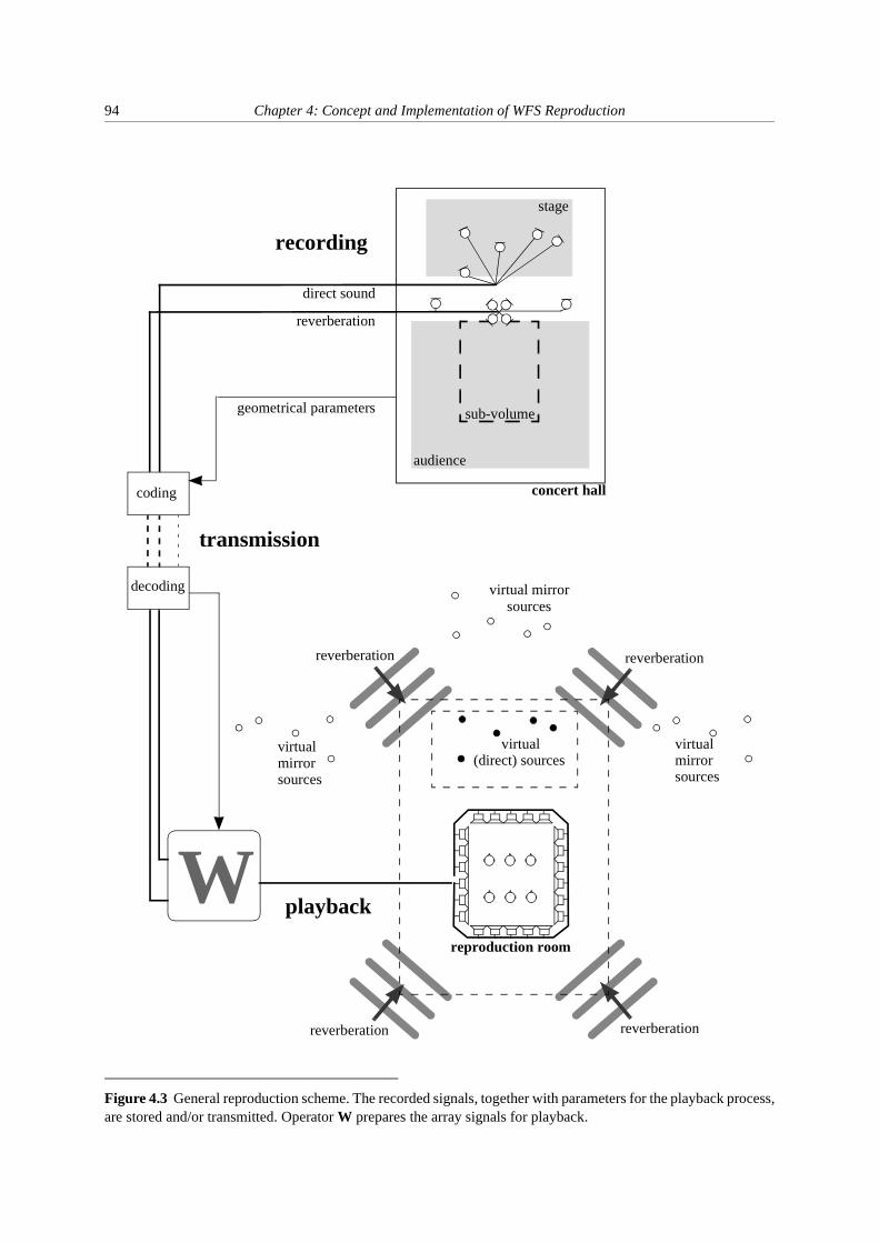
94 Chapter 4: Concept and Implementation of WFS Reproduction
Figure 4.3 General reproduction scheme. The recorded signals, together with parameters for the playback process,are stored and/or transmitted. Operator W prepares the array signals for playback.
concert hall
sub-volume
stage
audience
reproduction room
W
transmission
recording
playback
reverberation reverberation
reverberationreverberation
virtual mirrorsources
virtualmirrorsources
virtualmirrorsources
coding
decoding
direct sound
reverberation
geometrical parameters
virtual(direct) sources
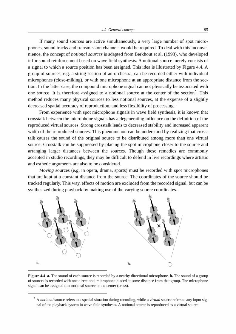
4.2 General concept 95
If many sound sources are active simultaneously, a very large number of spot micro-phones, sound tracks and transmission channels would be required. To deal with this inconve-nience, the concept of notional sources is adapted from Berkhout et al. (1993), who developedit for sound reinforcement based on wave field synthesis. A notional source merely consists ofa signal to which a source position has been assigned. This idea is illustrated by Figure 4.4. Agroup of sources, e.g. a string section of an orchestra, can be recorded either with individualmicrophones (close-miking), or with one microphone at an appropriate distance from the sec-tion. In the latter case, the compound microphone signal can not physically be associated withone source. It is therefore assigned to a notional source at the center of the section* . Thismethod reduces many physical sources to less notional sources, at the expense of a slightlydecreased spatial accuracy of reproduction, and less flexibility of processing.
From experience with spot microphone signals in wave field synthesis, it is known thatcrosstalk between the microphone signals has a degenerating influence on the definition of thereproduced virtual sources. Strong crosstalk leads to decreased stability and increased apparentwidth of the reproduced sources. This phenomenon can be understood by realizing that cross-talk causes the sound of the original source to be distributed among more than one virtualsource. Crosstalk can be suppressed by placing the spot microphone closer to the source andarranging larger distances between the sources. Though these remedies are commonlyaccepted in studio recordings, they may be difficult to defend in live recordings where artisticand esthetic arguments are also to be considered.
Moving sources (e.g. in opera, drama, sports) must be recorded with spot microphonesthat are kept at a constant distance from the source. The coordinates of the source should betracked regularly. This way, effects of motion are excluded from the recorded signal, but can besynthesized during playback by making use of the varying source coordinates.
* A notional source refers to a special situation during recording, while a virtual source refers to any input sig-nal of the playback system in wave field synthesis. A notional source is reproduced as a virtual source.
Figure 4.4 a. The sound of each source is recorded by a nearby directional microphone. b. The sound of a groupof sources is recorded with one directional microphone placed at some distance from that group. The microphonesignal can be assigned to a notional source in the center (cross).
a. b.

96 Chapter 4: Concept and Implementation of WFS Reproduction
Ambient microphones
In stereophony, the ‘main microphone pair’ (Section 1.6.3) is carefully positioned infront of the ensemble to obtain the desired place of phantom sources within the stereo image,and the desired balance between direct and reflective sound. In many cases these microphonesignals can also be used for reproduction by wave field synthesis, see Section 4.2.5. However,in the present concept, the term ‘main’ is not appropriate any more, because imaging for wavefield synthesis depends largely on the processing of spot microphone signals. Therefore,instead, the word ‘ambient’ is introduced to denote all microphone techniques that capture thereverberant sound for the purpose of wave field synthesis. Speaking in terms of impulseresponses, the ambient signals ideally consist of late reflections and reverberation. In practice,also direct sound and early reflections will be recorded, but these will not influence the repro-duced image if the direct/reverberation ratio is sufficiently low.
The need for recording techniques of ambient sound has grown strongly since the intro-duction of surround sound. A few techniques have already been proposed. The ambisonicreproduction method (Section 1.7.3) has encouraged the development of a four-channel coinci-dent microphone system with electronically controllable directivity and orientation (Sound-Field). Theile (1996) uses a four-channel ORTF-like microphone configuration intended foruse in 2/2 or 3/2 surround sound recordings (Figure 1.20b). Both microphone techniquesbelong to a special class of recording techniques based on the idea that sound must be recordedall around, because it arrives at the listener from all around. Figure 4.5a shows the general idea
ambientmicrophones
Figure 4.5 a. The sound field is recorded by directing the ambient microphones towards angular sectors of theacoustic space. The degree of correlation between the signals is determined by the radius of the circle of micro-phones and their directivity characteristics. During playback, the microphone signals are reproduced as planewaves along the dashed bisectors. Note that the radius of the microphone circle is zero for the SoundField micro-phone, and 15 cm in the ORTF-like configuration. With a cardioid directivity pattern, four sectors provide suffi-cient coverage. b. The directional error during playback depends on the listener position. The gray area is theangular sector of one particular microphone. The waves originating from sources 1 and 2 are reproduced as planewaves along the arrowed bisector. For a listener at the center, the directional error of these particular sources equalsα. For a listener off-center, the directional error is smaller as the source is further away: β2 < β1. Since late reflec-tions can be considered to originate from far-away mirror sources, this reproduction technique yields a fair recon-struction of these waves.
β1
α
β21
2
b.a.
center
off-center
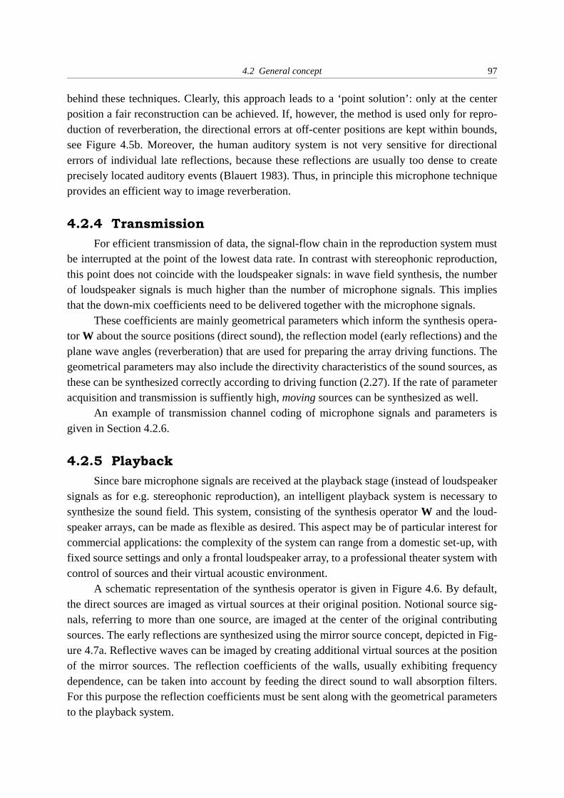
4.2 General concept 97
behind these techniques. Clearly, this approach leads to a ‘point solution’: only at the centerposition a fair reconstruction can be achieved. If, however, the method is used only for repro-duction of reverberation, the directional errors at off-center positions are kept within bounds,see Figure 4.5b. Moreover, the human auditory system is not very sensitive for directionalerrors of individual late reflections, because these reflections are usually too dense to createprecisely located auditory events (Blauert 1983). Thus, in principle this microphone techniqueprovides an efficient way to image reverberation.
4.2.4 Transmission
For efficient transmission of data, the signal-flow chain in the reproduction system mustbe interrupted at the point of the lowest data rate. In contrast with stereophonic reproduction,this point does not coincide with the loudspeaker signals: in wave field synthesis, the numberof loudspeaker signals is much higher than the number of microphone signals. This impliesthat the down-mix coefficients need to be delivered together with the microphone signals.
These coefficients are mainly geometrical parameters which inform the synthesis opera-tor W about the source positions (direct sound), the reflection model (early reflections) and theplane wave angles (reverberation) that are used for preparing the array driving functions. Thegeometrical parameters may also include the directivity characteristics of the sound sources, asthese can be synthesized correctly according to driving function (2.27). If the rate of parameteracquisition and transmission is suffiently high, moving sources can be synthesized as well.
An example of transmission channel coding of microphone signals and parameters isgiven in Section 4.2.6.
4.2.5 Playback
Since bare microphone signals are received at the playback stage (instead of loudspeakersignals as for e.g. stereophonic reproduction), an intelligent playback system is necessary tosynthesize the sound field. This system, consisting of the synthesis operator W and the loud-speaker arrays, can be made as flexible as desired. This aspect may be of particular interest forcommercial applications: the complexity of the system can range from a domestic set-up, withfixed source settings and only a frontal loudspeaker array, to a professional theater system withcontrol of sources and their virtual acoustic environment.
A schematic representation of the synthesis operator is given in Figure 4.6. By default,the direct sources are imaged as virtual sources at their original position. Notional source sig-nals, referring to more than one source, are imaged at the center of the original contributingsources. The early reflections are synthesized using the mirror source concept, depicted in Fig-ure 4.7a. Reflective waves can be imaged by creating additional virtual sources at the positionof the mirror sources. The reflection coefficients of the walls, usually exhibiting frequencydependence, can be taken into account by feeding the direct sound to wall absorption filters.For this purpose the reflection coefficients must be sent along with the geometrical parametersto the playback system.

98 Chapter 4: Concept and Implementation of WFS Reproduction
Figure 4.6 The synthesis operator W. The spot microphone signals for the direct sound unit are also used as inputfor the early reflections unit. Direct sound as well as early reflections are reconstructed as spherical waves, whilethe reverberation signals are reproduced as plane waves.
Figure 4.7 a. Mirror source model. If sound is reflected by a wall, the reflected waves correspond to that of afictive mirror source at the other side of the wall. In wave field synthesis, both the source and its mirror source aresynthesized as virtual sources. b. Plane wave synthesis of ambient microphone signals, including the stereo mainpair signals.
wallsource mirror source
b.a.
main left main right

4.2 General concept 99
The late lateral reflections, that are held responsible for a sense of envelopment (Bradleyet al. 1995), are incorporated in the reverberation signals by using the ambient microphonetechnique described in Figure 4.5. These waves are reproduced as plane waves along the origi-nal bisectors (Figure 4.7b). Artificial reverberation may serve as an alternative for recordedreverberation. The stereo ‘main’ pair signals, if available, can be reproduced similarly (see alsothe next sub-section).
Returning to Figure 4.6, it can be seen that all signals pass a set of equalization filtersbefore the actual synthesis takes place. The filter shape depends on the loudspeaker type andthe source position with respect to the arrays, as argued in Section 3.2. After synthesis, the pro-duced virtual source driving functions (spherical or plane waves) are added and, if necessary,spatially convolved according to Section 3.3.3.
The reproduction of moving sources is also possible in the present concept. Movingsources are important in virtual reality applications, because they create action and suspense bydrawing the listener into the scenery. In order to allow fast and smooth motion, a time-depen-dent synthesis operator W(t) must be used. This requires additional processing power, becausethe positions of the source as well as its mirror sources are altered continuously.
4.2.6 Compatibility
The compatibility issue is concerned with upward and downward compatibility to stereo-phony and 3/2 surround sound. In this application, upward compatibility is the possibility ofplaying back old program material on the new system. Downward compatibility refers to theway in which old systems can cope with program material developed for the new system.
A. Upward compatibility
Upward compatibility is obtained by applying the virtual loudspeaker concept. In thisconcept, some appropriately placed virtual sources are fed by the loudspeaker signals origi-nally meant for stereo or 3/2 surround.
For the stereo material, an equilateral triangle may be arranged (Section 1.6.1), but thiswould give the usual small listening area of two-channel stereophony. Instead, the stereo sig-nals can be reproduced by means of two far-away virtual loudspeakers. If these virtual loud-speakers are placed at infinity* , two plane waves angled ± 30º are produced (Boone et al. 1995,Geluk 1994), with several advantages:
1. the direction of the notional sources remains at ± 30º, independent of the listening position;
2. the intensity of the virtual loudspeakers is (almost) independent of the listening position;
3. the reproduced wave field is decoupled from the listening room: the wave fronts cannot beassociated with a realizable (point) source position within the room.
* Of course the corresponding infinite delay is omitted and sound level is kept at a reasonable height.

100 Chapter 4: Concept and Implementation of WFS Reproduction
With these advantages already a less critical sweet spot area is constructed. Nevertheless, theperceived image still shifts if the listener moves to the side, because in that case one signal willreach the listener before the other one does. The central phantom source (often a soloist or avoice-over) will gain stability by adding a virtual center cluster on the symmetry axis betweenthe virtual loudspeakers, as drawn in Figure 4.8. Such a central loudspeaker, which is regularlyapplied in theater sound systems (Bracewell 1993), is fed by the left and right stereo signals, butat a lower level to avoid coloration. Furthermore, the left and right channels are slightly delayedwith respect to the central channel. The precedence effect will then secure correct localization,while (comb filter) coloration is avoided or further reduced.
For 3/2 program material, the virtual loudspeakers of the left, right and surround chan-nels are imaged at infinity, at the standardized angles ± 30º and ± 110º. The center channel canbe routed to an appropriate center cluster position.
B. Downward compatibility
Downward compatibility can be achieved by special coding of the microphone signals.The synthesis operator W requires the bare microphone signals as inputs, while the stereo and3/2 surround systems need mixed signals. The stereo signals consist of main microphone sig-nals to which spot microphone signals are added by panning (Section 1.6.3). Since at presentthe 3/2 recording technique is still under development, a coding scheme for this material willdefinitely be premature, but an example scheme is given in Figure 4.9. This scheme assumesthat together with a stereo ‘main’ microphone pair, two additional ambient microphones areused (e.g. the reversed ORTF-pair drawn in Figure 1.20a). Inside the mixing console, anencoder keeps track of the routing paths and levels that will serve as a key to recover the origi-nal microphone signals for reproduction by wave field synthesis. The output of the decoder canbe connected to the synthesis operator W. The stripped L and R channels and the original S1and S2 channels are reproduced as ambient plane waves, while the spot microphone channelsare further processed to yield direct sound and early reflections using the geometrical parame-
L R
C
Figure 4.8 Virtual loudspeakers and a center cluster for stereophonic playback.

4.3 Laboratory demonstration system 101
ters. In this example, the C’ channel consists of merely spot microphone signals. Since thesesignals are transmitted individually, the C’ channel is not decoded for wave field synthesis.
4.3 Laboratory demonstration system
The playback concept of Section 4.2.5 formed the basis for the design of a demonstrationand research reproduction system. This system, that is described below, is installed in thereproduction room at the Delft Laboratory of Seismics and Acoustics.
4.3.1 Overview
Figure 4.10 depicts the playback scheme for the laboratory demonstration system. A dig-ital multi-track recorder provides up to 16 microphone signals that are mixed down to maxi-mally 8 input signals for the DSP-station. This station, that forms the synthesis operator W,produces the driving signals for a closed array surrounding the listening area, according to Fig-ure 4.2c. The heart of the station is formed by 8 digital signal processors (DSPs) that controlthe position of the virtual sources and the direction of the reverberant waves. Both the DSP-station and the loudspeaker arrays are custom-built by Duran Audio, Zaltbommel.
spo
tam
bien
t
‘main’
mixing key
L
R
C’
S1’S2’
virtualsources
geo.
coding decoding
stereo compatible;no decoding
3/2 surround compatible;subtract center channelfrom L and R channels
wave field synthesis;subtract all spot mic.signals from L and R
signal mixed according
bare microphone signal
to mixing key
param.
mixing key
spo
tam
bien
t
geo. param.
Figure 4.9 Coding scheme for downward compatibility. The primed channels belong to the 3/2 surround system.The central channel C’ may consist of one or more spot microphone signals. The L’ and R’ channels of the 3/2system are retrieved by setting L’ = L – 0.7 C’ and R’ = R – 0.7 C’. The wave field synthesis channels are recoveredby similar, but more complex, information enclosed in the mixing key.
transmission towards W from themicrophones
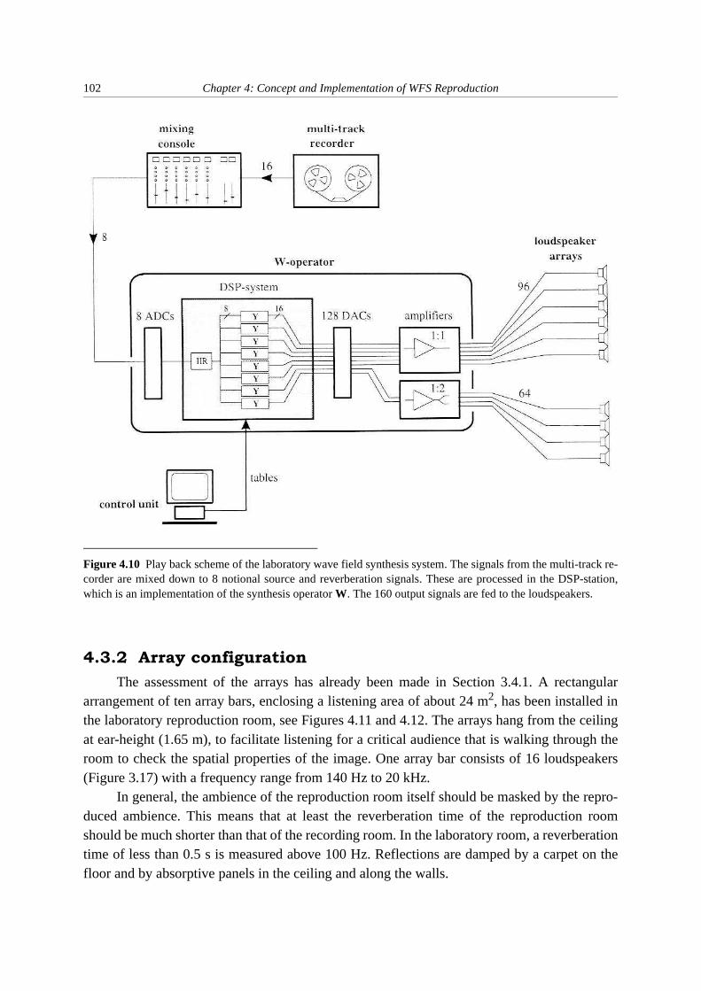
102 Chapter 4: Concept and Implementation of WFS Reproduction
4.3.2 Array configuration
The assessment of the arrays has already been made in Section 3.4.1. A rectangulararrangement of ten array bars, enclosing a listening area of about 24 m2, has been installed inthe laboratory reproduction room, see Figures 4.11 and 4.12. The arrays hang from the ceilingat ear-height (1.65 m), to facilitate listening for a critical audience that is walking through theroom to check the spatial properties of the image. One array bar consists of 16 loudspeakers(Figure 3.17) with a frequency range from 140 Hz to 20 kHz.
In general, the ambience of the reproduction room itself should be masked by the repro-duced ambience. This means that at least the reverberation time of the reproduction roomshould be much shorter than that of the recording room. In the laboratory room, a reverberationtime of less than 0.5 s is measured above 100 Hz. Reflections are damped by a carpet on thefloor and by absorptive panels in the ceiling and along the walls.
Figure 4.10 Play back scheme of the laboratory wave field synthesis system. The signals from the multi-track re-corder are mixed down to 8 notional source and reverberation signals. These are processed in the DSP-station,which is an implementation of the synthesis operator W. The 160 output signals are fed to the loudspeakers.
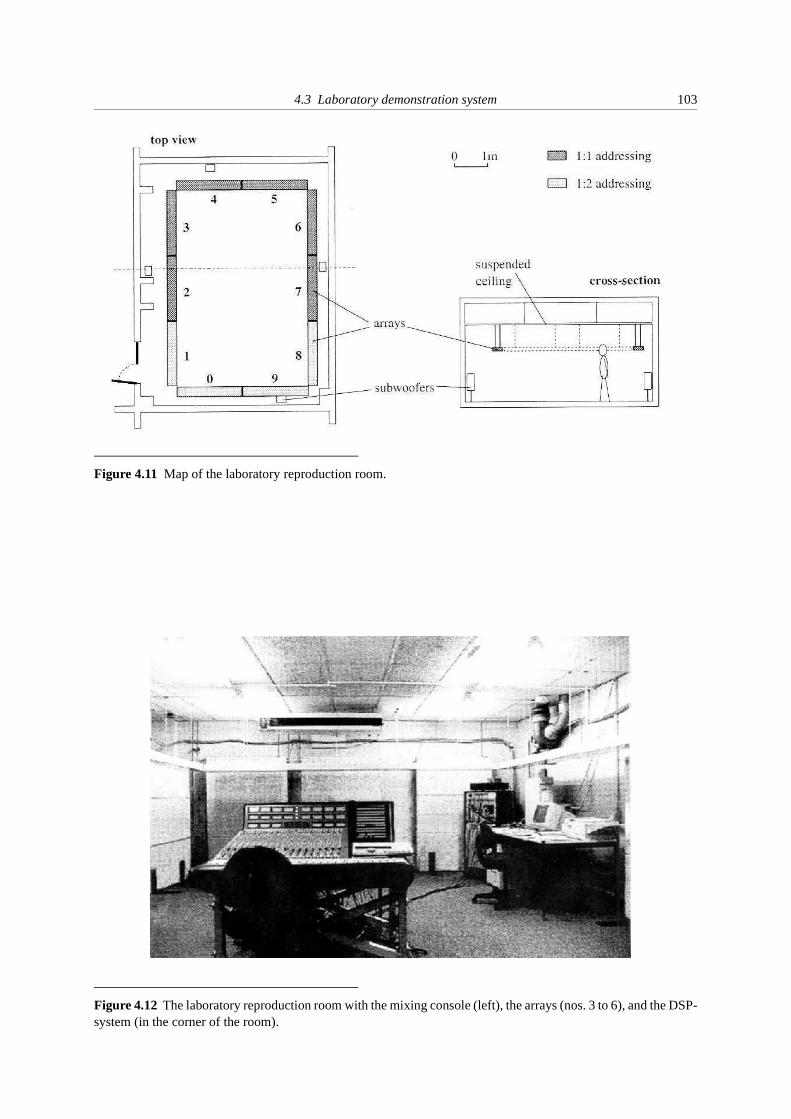
4.3 Laboratory demonstration system 103
Figure 4.11 Map of the laboratory reproduction room.
Figure 4.12 The laboratory reproduction room with the mixing console (left), the arrays (nos. 3 to 6), and the DSP-system (in the corner of the room).

104 Chapter 4: Concept and Implementation of WFS Reproduction
The frequency range below 140 Hz is supplied by free standing loudspeakers used assubwoofers (Philips DSS 930, described by Willems 1993). According to the spatial aliasingrequirement (2.35), the loudspeaker spacing for these woofers should not exceed 1.2 m. At thefrequency range of operation, however, the wave pattern in this room is dominated by standingwave modes, so that proper synthesis is impossible below 140 Hz. Therefore, a more efficientwoofer arrangement can be made without affecting quality of synthesis: each side is providedwith one woofer, for which the signals are taken from the middle array element of each bar atthe respective sides. For example, the front subwoofer receives the low-pass filtered signals( dB at 140 Hz, –24 dB/oct.) of the eighth elements of bar 4 and 5. Thus, the front woofersignal is a filtered addition of two signals, just like the rear woofer signal, whereas the sidewoofers are each supplied by three signals. As long as the sources keep away about 50 cmfrom the arrays, the variation in bass response between different source positions remainswithin an acceptable range.
4.3.3 DSP-system hardware
A DSP-system with 8 input and 128 output channels takes care of the processing of theloudspeaker signals. Each of the 8 floating point DSPs (TMS320C32) reads all 8 inputs andwrites 16 outputs. The actual number of virtual sources processed in real-time by one DSP is 4at 44.1 kHz sampling rate, or 6 at 32 kHz. This process, denoted Y, is modular in the sense thatthe number of DSPs running Y is proportional to the number of output channels.
A full coverage of the four sides of the reproduction room requires at least 160 loud-speakers, whereas the DSP-system hardware supports a maximum of 128 outputs. To copewith this discrepancy, it is reasoned that in normal use only reverberation and no direct soundwill be reproduced from the rear arrays, and this may be done with less spatial accuracy. There-fore, the following distribution is made: arrays 2 to 7 are addressed by one DSP each, or inother words, each of their loudspeakers is driven by an individual signal (denoted 1:1). Theremaining 4 rear arrays are driven in two-element subarrays (denoted 1:2), which may bethought of as a simple form of a spatial convolution filter (see Section 3.3.3). The use of subar-rays partly compensates the effects of the lower spatial aliasing frequency (with respect to thefront arrays), because it benefits the synthesis of waves with a small angle of incidence withrespect to the array.
The DSP-system is table-driven: a control unit (PC 486DX) calculates the synthesisparameters from the (new) virtual source positions entered graphically by the user.
4.3.4 DSP-system software
The gray box in Figure 4.10 shows that two different tasks are carried out by the DSPs:IIR-filtering and array signal processing Y. These tasks are related to the generalized monopoledriving function (2.30), which can be split in a frequency filter
, (4.1a)
3–
H ω( ) sign ζ( )k2πj
---------------------=

4.3 Laboratory demonstration system 105
with as defined in Section 2.3.3, and a loudspeaker signal operator
, (4.1b)
where rn is the distance from the virtual source to loudspeaker n. Loudspeaker signal Qn is nowretrieved by
. (4.2)
This operation is implemented in the time-domain for reason of efficiency. If a vector of arraydriving signals is defined as
, (4.3)
with qn(t) the inverse Fourier transform of Qn(ω), then the array driving signals are processed as
, (4.4a)
where denotes time-domain convolution, hIIR(t) is an infinite impulse response filter yet tobe designed, and Y is a vector operator with elements
. (4.4b)
First, the design of hIIR(t) is discussed and next operator Y is implemented for both staticand moving sources.
IIR-filter
Ideally, hIIR(t) is a time-domain version of filter (4.1a), which has a slope of +3 dB peroctave, see also Section 3.2.2. This filter is however not applicable above the spatial aliasingfrequency, where no constructive interference of individual loudspeaker contributions occurs.It appears to be possible to design a single filter that renders a reasonably flat system responsefor a large range of virtual source positions and a large listening area. The filter, shown in Fig-ure 4.13, is designed by equalizing the average response of a number of virtual sources andreceiver positions in the reproduction room. In this option the loudspeaker response is compen-sated as well. A cardioid microphone was used as receiver to suppress reflections in the mea-sured signals. In agreement with theory, a positive slope of a few dB per octave is visible, apartfrom a peak at 400 Hz due to a broad dip in the loudspeaker response (compare Figure 3.22).No attempt is made here to match the IIR-filter’s phase response to the theoretical frequency-independent value of 45º for virtual sources behind the array, or –45º in front of the array. Ifdesired, these phase shifts can be controlled by applying an appropriate FIR-filter* instead.
ζ zR zS⁄=
Ynζ
ζ 1–----------- ϕn
sign ζ( )jkrn( )exp
rn
------------------------------------------cos=
Qn ω( ) YnH ω( )S ω( )=
q t( ) q1 t( ) … qn t( ) … qN t( )T
=
q t( ) Y t( )* hIIR t( )* s t( )[ ]=
*
Yn t( ) ζζ 1–-----------
ϕcos n
rn
---------------δ t sign ζ( )rn c⁄+( )=

106 Chapter 4: Concept and Implementation of WFS Reproduction
Synthesis of static sources
The task of the operator Y is to apply the correct delay and weighting coefficients fromM filtered input signals to N output signals. If the input signals are written as a source vector
, (4.5)
then the vector operator Y can be extended to a matrix operator Y yielding array driving signals
, (4.6)
where again denotes time-domain convolution, and the elements of Y are given by
, (4.7a)
with weighting coefficients
, (4.7b)
and time delays
. (4.7c)
Note that an extra delay τ0 > 0 has been introduced to avoid non-causality in case sign(ζm) = +1(for sources in front of the array). The delay and weighting coefficients are calculated in the con-trol unit. The delay values are derived from the distance between loudspeaker and virtualsource. The weighting coefficients anm depend on the position of the reference line R (see e.g.
* Finite impulse response filters generally require much more computation power of the DSPs.
Figure 4.13 Filter design based on the average measured response of virtual sources. The zeros (°) and poles (×)of the filter in the complex z-plane are shown to the right.
s t( ) s1 t( ) … sm t( ) … sM t( )T
=
q t( ) Y t( )* hIIR t( )* s t( )[ ]=
*
Ynm t( ) anmδ t τnm–( )=
anm
ζm
ζm 1–---------------
ϕcos nm
rnm
------------------=
τnm τ0 sign– ζm( )rnm
c--------=

4.3 Laboratory demonstration system 107
Figure 2.7 and Figure 2.17) via the ratio . For a straight linear array, the referenceline at z = zR is usually chosen parallel to the array in the middle of the listening area. For a lineararray with corners, e.g. the rectangular array of Figure 4.11, a single parallel reference line isimpossible. A solution is found in applying driving function (2.32b), which permits non-parallelreference lines to be used. By writing , the same form is obtained as in (2.30). Figure4.14 illustrates the assessment of the reference line for cornered arrays.
Not all array bars are active for a certain virtual source. At most, half of the array bars are‘seen’ by a virtual source, and in many situations it suffices to process even less loudspeakersignals. Figure 4.15 shows that much processing power can be saved by considering that notall positions within the rectangle will be occupied by listeners. Though a number of six virtualsources per array remains the limit in the laboratory demonstration system, an effective use ofprocessing power makes it possible to reproduce much more virtual (mirror) sources in total,all around the listening space. For this purpose a coding map has been set up manually, seeFigure 4.16. The virtual source area is divided in a large number of squares, the field code ofwhich specifies the array bars that are active for a virtual source within that square. Note thatno virtual sources can be placed in the blank middle area. This area is excluded for virtualsources, because listeners are not allowed to reside between active arrays and focused sources.
The delay coefficients produced by the control unit are rounded to the nearest integertime sample interval. For example, if a delay of 15.6 samples is calculated for a certain virtualsource m and loudspeaker n, the actual delay is set to 16 samples. At 32 kHz sample rate, themaximum phase error made in this way is 7.5º for the spatial aliasing frequency of 1340 Hz.Synthesis of wave fronts is therefore hardly influenced by this approximation.
ζ zR zS⁄=
∆r r⁄ ζ=
Figure 4.14 Choice of the reference line R in a cornered array configuration. a. The ratio ζ = ∆r/r must be contin-uous along the arrays to avoid discontinuous amplitudes along the synthesized wave fronts. If two reference lines(parallel to the respective arrays) are used, the ratio ∆r/r will in general be discontinuous at the corner. b. If onlyone, but fixed, reference line is used, not all stationary phase points at the array are defined: the arrows drawn donot cross the chosen reference line. The loudspeaker driving function is therefore not defined at position 1 and 2.c. Each virtual source S defines its own reference line, all of which intersect the center C of the listening area. Ref-erence line R is defined as the line through C, perpendicular to the line connecting S and C. A useful alternative isreference line R', which is the arc through C, centered around S. In real-time processing, using R' instead of Rspeeds up the calculation of ζ/(ζ–1). Therefore R' is employed in the laboratory system, with C at the middle of therectangular array configuration.
R1
R2
arrays
R
a. b. c.
source
R
R'
r
∆rwave
front
C
S
∆r
r
1
2

108 Chapter 4: Concept and Implementation of WFS Reproduction
Figure 4.15 a. A virtual source near the corner ‘sees’ half of the arrays. b. If the region near the arrays is excludedfor listeners, only a small part of the arrays needs to be active.
a. b.
listening area
active arrays
passive arrays
Figure 4.16 Coding map used by the control unit to assign arrays to virtual sources. Each field code consists ofthree or less digits that indicate the array bars that are involved in synthesis of virtual sources present in that par-ticular field. Virtual sources outside the map are treated corresponding to the nearest field code. As an example,the area belonging to array bar 4 is shaded: only virtual sources within this area are assigned to array bar 4. Thecoding map, which allows efficient use of processing capacity, is initialized according to the geometry of the arrayand the desires of the user.

4.3 Laboratory demonstration system 109
Virtual mirror sources are treated by the DSP-system in the same manner as virtualdirect sources. The mirror source positions and strengths are calculated in the control unit.About 5 to 15 virtual mirror sources, each with a delay time up to 65 ms, can be generated fora single virtual source, depending on the number and positions of the other virtual sources.Frequency-dependent absorption can be incorporated by reserving input channels with adjust-able IIR-filters for the mirror source signals.
Synthesis of moving virtual sources
Moving sources require a different treatment by the control unit and DSP-system. Eachsample period, an update of delay and weighting coefficients is necessary. For this reason,(4.7b) and (4.7c) become time-dependent (Jansen 1997):
, (4.8a)
, (4.8b)
where .Because the control unit can only update the delay and weight tables a few times per sec-
ond* , the DSPs must take over some calculation tasks from the control unit. An efficient com-putation method is described by Jansen (1997). The control unit periodically transfers thecoordinates and weight tables of certain support points to the DSPs, together with a speedparameter, see Figure 4.17. The coordinates are used to compute rnm(t) along the linearizedpath. The delays, calculated from rnm(t), are not rounded to the nearest integer like for staticsources, because these irregularities become audible as sputtering. This problem is solved byresampling or interpolation between the nearest time samples.
The weight tables along the path are computed through linear interpolation between theweight tables of the support points. This method saves much processing time in comparison tothe exact calculation of anm(t) from the coordinates of the support points.
* The rate of table-updating is limited by the time it takes for the control unit to compute a table.
anm t( )ζm t( )
ζm t( ) 1–----------------------
ϕcos nm t( )
rnm t( )-------------------------=
τnm t( ) τ0 sign– ζm t( )( )rnm t( )
c r·nm
t( )+------------------------=
r·nm
t( ) rnm t( ) td⁄d=
Figure 4.17 A moving source can be processed by interpolating between support points along the source path.
array
pathsupport points
approximated path
n
rnm
m

110 Chapter 4: Concept and Implementation of WFS Reproduction
Note that the weights are estimated with much less accuracy than the delays. The differ-ence in precision of calculation is motivated by perceptual considerations. The perceiveddirection of the source is mainly determined by the distribution of delay coefficients along thearrays. If accurate localization is appreciated and round-off errors should not be audible, thecomputation of delays must be done with great precision. The perceived sound level of thesource depends on the weighting coefficients. Since level fluctuations of a few dB are hardlyaudible, medium precision is allowed in generating weight tables. By using linear interpolationbetween weight tables, smooth level variations along the path are guaranteed.
4.4 Applications of the new concept
The presented laboratory system is one implementation of the concept, but other imple-mentations are also possible. In Section 4.2, already some considerations have been madeabout simpler as well as more enhanced systems for sound reproduction. In this section, a moredetailed discussion is given, where the laboratory system serves as a reference.
4.4.1 Living-room
For domestic use, the design described above is perhaps too sophisticated in softwareand hardware. A few simplifications are still possible, leaving the overall performance more orless unaffected. Of course, the general purpose DSPs can be captured in a dedicated chip,which will lead to much lower production costs. Also, the number of channels can be restrictedby allowing yet a larger spacing of array loudspeakers at the back and sides, if no direct virtualsources are imaged in those directions. Concerning the integration of the arrays into the inte-rior of the living-room, it should be noted that the radiated sound of the arrays should not beshielded by objects in the ‘line of sight’. Built-in arrays (into the walls just beneath the ceiling)or foldaway arrays (towards the ceiling or walls) might be feasible. It should also be mentionedthat the exploration of array technology has just begun: special array designs, such as the light-weight transparent electrostatic strips in Section 3.4.2, may further improve chances for thepractical implementation of arrays.
The main question for acceptance of the novel reproduction method in the living-room iswhether the advantages of the wave field synthesis system outweigh its higher price and itsmore complicated requirements for installation. The history of sound reproduction proves thatcompatibility with previous and contemporary reproduction systems is of primary interest inanswering this question. Commercial chances are raised if the new system offers a clearimprovement in reproducing conventional program material. Preliminary listening tests withthe proposed method of reproducing two-channel stereo material (Section 4.2.6) yieldedalready a striking enhancement of the spatial image. Together with a modular set-up of thearrays and the synthesis operator, this might be the basis for an introduction of the system tothe consumer market.

4.4 Applications of the new concept 111
4.4.2 Cinema
In cinemas, loudspeaker arrays usually do not have to compete with furniture, as in adomestic environment. The arrays can be built into the back and side walls, and behind thefront screen. With a playback system based on wave field synthesis, surround sound effects arenot restricted any more to the position of the surround loudspeakers: sound can be created allaround the audience, with a much more realistic spread. Since the input channels of the systemconsist of discrete source signals with source coordinates, the sound image can be adjusted tothe shape or size of the cinema.
4.4.3 Virtual reality theater
A virtual reality system is an interactive device that evokes an image to the user which isvery close to reality, by stimulating all his senses in a consistent way. The concept of wavefield synthesis lends itself admirably to this purpose, because of its ability to create any desiredsound field from a few parameters. Since the listening area is basically unlimited, the user hasa large freedom of movement. In this way, several users can use the system simultaneously.The ultimate virtual reality system consists of 2D loudspeaker arrays behind an acousticallyand visually transparent screen, producing a full 3D sound image. Especially the possibility tofocus sources in front of the array will contribute to a thrilling experience.
4.4.4 Simulators
Closely related to virtual reality systems are (flight-)simulators. Instead of an excitingsituation, an unusual situation is recalled here, to which the trainee must react in an appropriateway. Also in these training devices a realistic image must be created, so the requirements arevery similar to those for the virtual reality theater.
4.4.5 Acoustic research
Of course, the laboratory system is also extraordinarily suited for room acoustic and psy-cho-acoustic research. Except the acoustic design of newly built concert-halls, also the effectsof renovation of existing halls can be modeled and judged in advance. Because of the listener’sfreedom to move and the possibility to directly deliberate with others, this way of modeling isfar more natural and convenient than binaural modeling, which is proposed alternatively.
Spatial perception research is much facilitated by using the laboratory system. In earlierresearch, sources were represented by loudspeakers placed at positions allowed by the dimen-sions of the room. In wave field synthesis, sources are placed under software control at anydistance from the subject. Especially, research on the perception of moving sources willbecome much easier.

112 Chapter 4: Concept and Implementation of WFS Reproduction
4.5 Conclusions
The general concept of sound reproduction by wave field synthesis is developed by con-sidering the natural sound field in its acoustic environment. The wave field inside a certainenclosure within that environment is determined by the Kirchhoff-Helmholtz integral appliedat the boundary of that enclosure. Theoretically, a physical copy of the original sound field canbe synthesized in the reproduction room. In order to come to a practical implementation of theconcept, a number of data compression and data reduction steps is necessary. The proposedreproduction method makes it possible to reproduce the natural sound field as well as producean ideal or artificial sound field from the same program material.
Three phases are distinguished in sound reproduction: the recording phase, the transmis-sion and/or storage phase, and the playback phase. In the first phase, spot microphones areused to record the direct sound and so-called ambient microphones are used to capture thereverberant sound. These signals are transmitted or stored together with relevant geometricalparameters telling the playback system how to reproduce the sound field. Eventually, the directsound is processed for virtual sources. The early reflections are reproduced by assigning thedirect sound to virtual mirror sources. The reverberation is created by plane wave synthesis ofthe ambient microphone signals.
The general concept is realized in a laboratory wave field synthesis system. This systemcomprises a digital signal processing unit, which is an implementation of the synthesis opera-tor, and a rectangular array configuration surrounding the listeners. Any multi-track materialcan be reproduced, while the recorded sources may be imaged in their original environment orin a non-existing or yet to be built concert-hall. Sources can be placed anywhere, even withinthe listening area by means of focusing techniques. Therefore the system is also very interest-ing for virtual reality theaters and simulators.

113
Chapter 5
Objective Evaluation
5.1 Introduction
In this chapter, the laboratory wave field synthesis system is evaluated by means ofobjective measurements. This evaluation consists of two parts: the calibration of the systemresponse, which illustrates the temporal and spatial characteristics of virtual sources, and anobjective comparison of the new reproduction system in relation to stereophony and surroundsound. Besides well-known qualification methods, such as frequency characteristics and soundpressure levels, also less customary methods are used in determining differences in reproduc-tion quality. The ins and outs of these methods are discussed extensively. Next, these methodsare applied to the evaluation of reproduction of direct sound, early reflections and reverbera-tion separately.
5.2 System response
The temporal and spatial performance of the laboratory reproduction system is deter-mined by measuring the impulse response for several virtual source positions. With these data,the equalization filter of the system can be calibrated and the spatial accuracy of reproductioncan be verified.

114 Chapter 5: Objective Evaluation
5.2.1 Frequency response
The frequency response of the laboratory system is measured to check the design of theequalization filter and the subwoofer arrangement. By placing virtual sources at different dis-tances, also the 1/r-dependence of the sound level is checked. Reflections of the reproductionroom are expected to influence only the fine-structure of the measured spectra, except in thelow frequency range where standing waves become important.
Figure 5.1 shows the frequency response of six virtual sources in the reproduction room.Virtual sources 1 and 2 were focused in front of the array. The distances of the virtual sourcesto the measurement microphone are 0.5, 1, 2, 4, 8 and 16 m, respectively. Between real sourcesat these increasing distances, a sound level reduction of 6 dB is expected. The results show thatthis theoretical value is approximated fairly well for virtual sources 4 to 6, while it is less than6 dB for the others. This deviation is a result of the use of linear arrays, for which the 1/r-lawis only valid at the reference position (position C in Figure 4.14). In practice, these small devi-ations will hardly be audible. Besides, the actual levels are easily overruled by the gain controlon the mixing console.
The (internal) variation of the responses remains within ±3 dB for frequencies above 300Hz. Below this frequency, standing wave patterns dominate the results.
5.2.2 Spatial response
The spatial behavior of the wave fields of virtual sources is investigated in an anechoicroom. The measurement microphone is displaced stepwise along an acquisition line parallel tothe array. The measurements and simulations of Figure 5.2 show that the wave fields of
Figure 5.1 System response of virtual sources at positions 1 to 6, as shown on the map to the right. Only the frontpart of the rectangular array configuration is drawn. The receiver position is at the cross (×). Since the distancedoubles between subsequent source-receiver combinations, an offset of 6 dB is expected between subsequent spec-

5.2 System response 115
focused and non-focused virtual sources are well controlled, i.e. their spatial behavior is ingood agreement with theory. Small differences can be ascribed to the frequency response anddirectivity characteristics of the loudspeakers.
Some effects of spatial aliasing are visible for the virtual source behind the array (Figure5.2a), while they are more or less absent for the virtual source in front of the array. This pre-sumption can be verified by making a plane wave decomposition of the measured data sets, seeFigure 5.3. Above the horizontal dotted lines in the diagrams the plane wave components areobviously aliasing-free. Note that the aliased wave fronts appear at higher values of k in thefocused wave field, which seems to be in contradiction to the spatial aliasing condition being
a. b.
Figure 5.2 Measurement and simulation of a Gaussian wave front of a virtual source in the xt-domain. a. Virtual source at 1 m behind the array. b. Virtual source at 1 m in front of the array (focused source). The 32 element array is at a distance of 3 m parallel to the acquisition line. Bandwidth: 0.1 - 2.5 kHz.
simulationmeasurement simulationmeasurement
Figure 5.3 2D-Fourier transform or kxk-diagram of the measured data of Figure 5.2. a. Virtual source at 1 m behind the array. b. Virtual source at 1 m in front of the array (focused source). The interference pattern, seen at high values of k, is typical for aliased wave fields. Bandwidth: 0 - 6.8 kHz.
a. b.
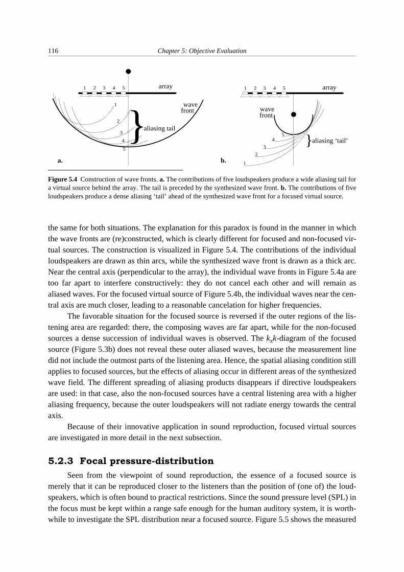
116 Chapter 5: Objective Evaluation
the same for both situations. The explanation for this paradox is found in the manner in whichthe wave fronts are (re)constructed, which is clearly different for focused and non-focused vir-tual sources. The construction is visualized in Figure 5.4. The contributions of the individualloudspeakers are drawn as thin arcs, while the synthesized wave front is drawn as a thick arc.Near the central axis (perpendicular to the array), the individual wave fronts in Figure 5.4a aretoo far apart to interfere constructively: they do not cancel each other and will remain asaliased waves. For the focused virtual source of Figure 5.4b, the individual waves near the cen-tral axis are much closer, leading to a reasonable cancelation for higher frequencies.
The favorable situation for the focused source is reversed if the outer regions of the lis-tening area are regarded: there, the composing waves are far apart, while for the non-focusedsources a dense succession of individual waves is observed. The kxk-diagram of the focusedsource (Figure 5.3b) does not reveal these outer aliased waves, because the measurement linedid not include the outmost parts of the listening area. Hence, the spatial aliasing condition stillapplies to focused sources, but the effects of aliasing occur in different areas of the synthesizedwave field. The different spreading of aliasing products disappears if directive loudspeakersare used: in that case, also the non-focused sources have a central listening area with a higheraliasing frequency, because the outer loudspeakers will not radiate energy towards the centralaxis.
Because of their innovative application in sound reproduction, focused virtual sourcesare investigated in more detail in the next subsection.
5.2.3 Focal pressure-distribution
Seen from the viewpoint of sound reproduction, the essence of a focused source ismerely that it can be reproduced closer to the listeners than the position of (one of) the loud-speakers, which is often bound to practical restrictions. Since the sound pressure level (SPL) inthe focus must be kept within a range safe enough for the human auditory system, it is worth-while to investigate the SPL distribution near a focused source. Figure 5.5 shows the measured
wave
1 2 3 4 5
1
2
3
45
aliasing ‘tail’
1 2 3 4 5
aliasing tail1
2
3
4
5
wavefront
front
array array
Figure 5.4 Construction of wave fronts. a. The contributions of five loudspeakers produce a wide aliasing tail fora virtual source behind the array. The tail is preceded by the synthesized wave front. b. The contributions of fiveloudspeakers produce a dense aliasing ‘tail’ ahead of the synthesized wave front for a focused virtual source.
a. b.

5.2 System response 117
and simulated distributions. The SPL data at the left were taken in a 0.5 m2 area in the horizon-tal plane in an anechoic room; the simulation result is shown at the right. For visualization,cubic interpolation is used between the grid points, both for the measured and simulated dataset. A very good resemblance is obtained between measured and simulated data, confirmingthat the sound field produced by the arrays is well-controlled. A maximum pressure level of91.8 dB is measured in the small white area in the middle. At 0.45 meter beyond the focus(bottom of picture), it is 7 dB less, while to the side a minimum of 73.4 dB is reached.
The focal area is not restricted to the horizontal plane. This can be understood by firstconsidering a linear array of monopole loudspeakers, driven by the focusing operator. Figure5.6a shows that this array produces a focal circle in the plane perpendicular to that array. Ifloudspeakers with high directivity in the vertical plane are used, most of the energy radiated isconcentrated in the intersection point of the focal circle and the horizontal plane in front of thearray (Figure 5.6b). The main benefit of this is that strong reflections from floor and ceiling ofthe reproduction room will be prevented. In addition, a more efficient power consumption isachieved. Both advantages also apply to non-focused sources.
Figure 5.5 Sound pressure levels near a focus at 1 m from a 32 element array (bandwidth 0 - 2 kHz; ∆x = 12.7 cm).a. Left half: measurement in anechoic room, right half: simulation (with monopole loudspeakers). b. View of the situation. The SPL measurements are taken on a 60 point grid in the left half of the area.
a.
x
b.
array
area
(0,0)z
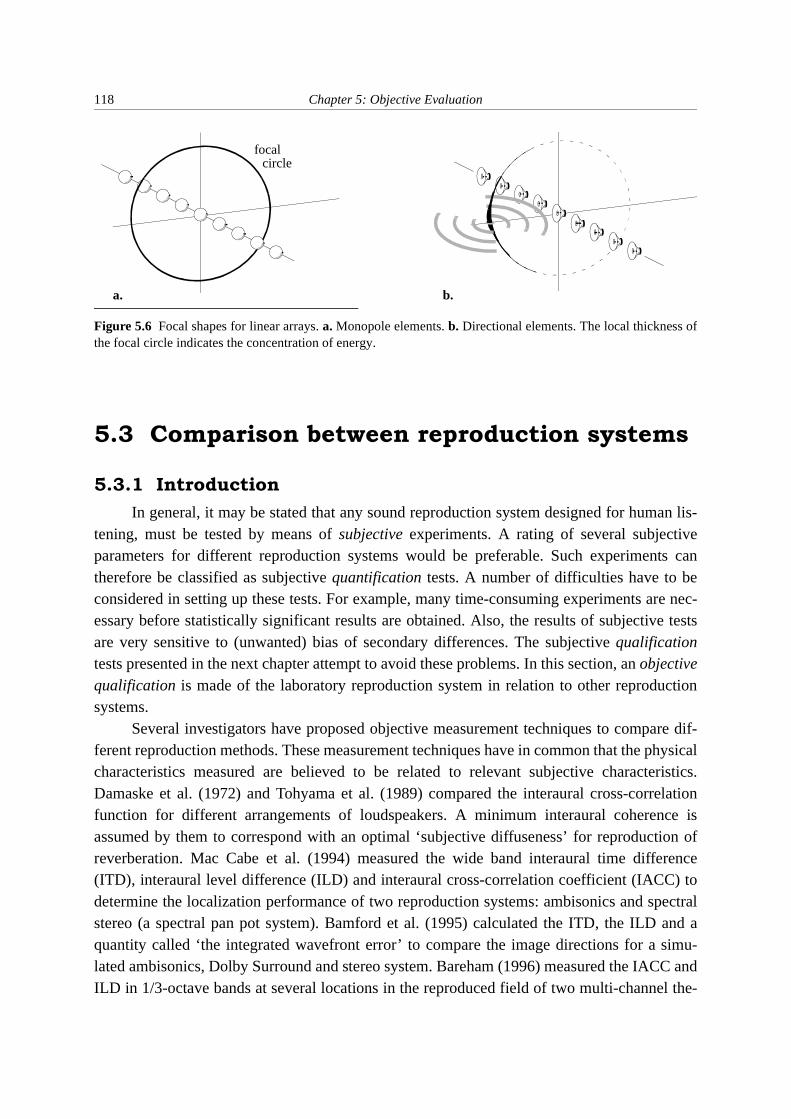
118 Chapter 5: Objective Evaluation
5.3 Comparison between reproduction systems
5.3.1 Introduction
In general, it may be stated that any sound reproduction system designed for human lis-tening, must be tested by means of subjective experiments. A rating of several subjectiveparameters for different reproduction systems would be preferable. Such experiments cantherefore be classified as subjective quantification tests. A number of difficulties have to beconsidered in setting up these tests. For example, many time-consuming experiments are nec-essary before statistically significant results are obtained. Also, the results of subjective testsare very sensitive to (unwanted) bias of secondary differences. The subjective qualificationtests presented in the next chapter attempt to avoid these problems. In this section, an objectivequalification is made of the laboratory reproduction system in relation to other reproductionsystems.
Several investigators have proposed objective measurement techniques to compare dif-ferent reproduction methods. These measurement techniques have in common that the physicalcharacteristics measured are believed to be related to relevant subjective characteristics.Damaske et al. (1972) and Tohyama et al. (1989) compared the interaural cross-correlationfunction for different arrangements of loudspeakers. A minimum interaural coherence isassumed by them to correspond with an optimal ‘subjective diffuseness’ for reproduction ofreverberation. Mac Cabe et al. (1994) measured the wide band interaural time difference(ITD), interaural level difference (ILD) and interaural cross-correlation coefficient (IACC) todetermine the localization performance of two reproduction systems: ambisonics and spectralstereo (a spectral pan pot system). Bamford et al. (1995) calculated the ITD, the ILD and aquantity called ‘the integrated wavefront error’ to compare the image directions for a simu-lated ambisonics, Dolby Surround and stereo system. Bareham (1996) measured the IACC andILD in 1/3-octave bands at several locations in the reproduced field of two multi-channel the-
Figure 5.6 Focal shapes for linear arrays. a. Monopole elements. b. Directional elements. The local thickness ofthe focal circle indicates the concentration of energy.
a. b.
focalcircle

5.3 Comparison between reproduction systems 119
ater systems. The IACC is here assumed to indicate the spaciousness of the sound field, whilethe ILD should provide information of the image direction.
Caution is needed in interpreting the aforementioned interaural parameters. For a naturalsound source in an enclosure, there is usually a well-defined relation between these parametersand the subjective attributes source direction and spaciousness. However, reproduction sys-tems generally do not produce natural sound fields: e.g. a stereophonic phantom source causesseveral maxima in the cross-correlation function measured at a dummy head. Therefore, inaddition, different measurement techniques have been proposed to qualify the reproducedsound fields (Boone et al. 1997). These are listed in Table 5.1, together with the objective andmain subjective attributes to which they are related.
These techniques, which will be explained in the next subsections, can be applied to thedirect sound, early reflections and reverberation. For the purpose of comparison, these compo-nents are reproduced separately by the reproduction systems under investigation: wave fieldsynthesis, 3/2 surround and (two-channel) stereophony. Note that the IACC is not incorporatedin the table as a measure for spaciousness. It has been considered that it is awkward to use thismeasure in absence of a relevant reference situation. Instead, the intensity measurements areemployed to gain insight in the distribution of reflective sound.
The measurement environment is the reproduction room where the wave field synthesissystem has been installed (Figure 5.7). The stereo system shares the L and R loudspeakers withthe 3/2 surround system. These individual loudspeakers (Philips DSS 930) are placed some-what lower than the arrays (tweeters at 1.5 m above floor), at a circle of 2.75 m around the ori-gin. The surround loudspeakers SL and SR are placed at angles ±125º and a radius of 2.4 m,though the 3/2 standard specifies ±110º with the same radius as the front loudspeakers. Thisdeviation is imposed by the dimensions of the reproduction room. A smaller radius for allloudspeakers would have been possible, but then the listening area for 3/2 surround and stereowould become narrower. It will be shown that no serious affection of the 3/2 surround qualityis caused for those situations in which the surround loudspeakers are active.
Table 5.1 Sound field qualification techniques
Qualification technique Objective attributes Subjective attributes
Dummy-head measurements ILDs and ITDs Direction
Multi-trace impulse responses Shape of wave front Direction and distance
Intensity measurements Intensity distributions Direction, spaciousness, diffuseness
Frequency spectrum measurements 1/3-octave band spectra Coloration

120 Chapter 5: Objective Evaluation
5.3.2 Dummy-head measurements
The ILD and ITD are calculated from the impulse responses and measured atthe entrance of the left and right ear channel of a human or dummy head. The ILD is given by
. (5.1)
Since ILDs originate from frequency-dependent diffraction effects around the head, it is cus-tomary to determine them in frequency bands. Therefore, the ear signals are filtered in 1/3-oc-tave bands before evaluating Equation (5.1).
The ITD is the travel-time difference between sound arriving at the left and right ear. Itcan be determined by evaluating the wide band interaural cross-correlation function (Ando1985)
. (5.2)
The value of τ where Φrl is at its maximum, represents the time lag (ITD) between the ear sig-
Figure 5.7 Measurement situation for objective comparison between wave field synthesis (arrays), 3/2 surround(L, R, C, SL, SR) and stereophony (L, R). The top view also shows the position of the furniture in the room.
sl t( ) sr t( )
ILD 10sr t( )2
td∫sl t( )2
td∫---------------------log=
Φrl τ( ) 1
2T------ sr
T–
T
∫T ∞→lim t( )sl t τ+( )dt=

5.3 Comparison between reproduction systems 121
nals, arising from the path length difference from the source to either ear. For a real source inan anechoic environment, the measured Φrl contains only one distinct peak (Figure 5.8a). Thispeak occurs in the interval ms because of the limited path length difference. If the sourceis present in a reflective environment, multiple peaks occur (Figure 5.8b). Only the peak belong-ing to the direct sound falls in the range ms, unless the source is very close (within a fewdm) to a reflecting wall. Therefore, the ITD belonging to the direct sound of the source can usu-ally still be determined in a reflective environment.
A different situation exists for sound reproduction systems. Here, the actual sources arethe loudspeakers, rather than the phantom or virtual sources that are evoked. If the loudspeakersignals correlate in some degree, the interaural cross-correlation function will contain severallocal maxima (even if reflections are absent). In some cases, more than one distinct peak mayappear within the specified range of ms. In these cases, the image direction perceivedcan not be predicted easily. However, because the auditory system applies a frequency analysisto the ear signals before a kind of cross-correlation process is carried out (e.g. Stern et al. 1978,and Raatgever et al. 1986), it makes sense to observe the ITDs in frequency bands. Therefore,just like with the ILDs, the ear signals are filtered in 1/3-octave bands before determining theITDs. Only the direct sound will be considered: reflections from the reproduction room arewindowed off carefully, as a way to account for the precedence effect (Macpherson 1991). Itwill be shown here that the spectrally unraveled ILDs and ITDs provide interesting informa-tion on the frequency dependence of the reproduction quality.
Two sources without reflections are imaged by the reproduction systems, see Figure 5.8c.For reference and comparison, the response of a real source in an anechoic room is measured
τ 1≤
τ 1≤
Figure 5.8 a. Normalized interaural cross-correlation function for a real source at 45º in an anechoic room. b. Nor-malized interaural cross-correlation function for a real source at about 45º in the reproduction room of the DelftLaboratory of Seismics and Acoustics. c. Two sources a and b are imaged by the reproduction systems. The dummyhead locations are numbered 1 and 2.
τ 1≤

122 Chapter 5: Objective Evaluation
as well. Both the stereo and 3/2 surround system are supposed to use the same stereo imagingtechnique in this case: the central and rear loudspeakers are not in use here for 3/2 surround* .The signals for the L and R loudspeaker are identical for source a. The signals for source b areobtained by simulating an ORTF-pair at the center of the reproduction room (position 1). Forthe wave field synthesis system (hereafter: WFS system), sources a and b are reproduced asvirtual sources at the corresponding position. The head and torso simulator is a KEMAR(Burkhard at al. 1975).
Figure 5.9 compares the results for source a and listening position 1 of the reference (realsource), the stereo system and the WFS system. For this symmetrical listening geometry, thereal source was expected to render zero ILDs and ITDs. The non-zero ILDs at the high fre-quencies are probably caused by asymmetries of the head and torso simulator. The stereo
* Source a is assumed not to represent a soloist or voice-over, otherwise it could have been imaged by only employing the central loudspeaker of the 3/2 surround system. The C and S loudspeakers are not drawn for this system. Some pioneers of 3/2 surround mixing actually use only a 2/2 surround system for best results, thereby omitting the central loudspeaker (Theile 1996, and Scholtze 1997).
Figure 5.9 ILDs and ITDs for source a and dummy head position 1.a. Real source in anechoic room. b. Two-channel stereophony. c. Wave field synthesis.
interaural level differences interaural time differences
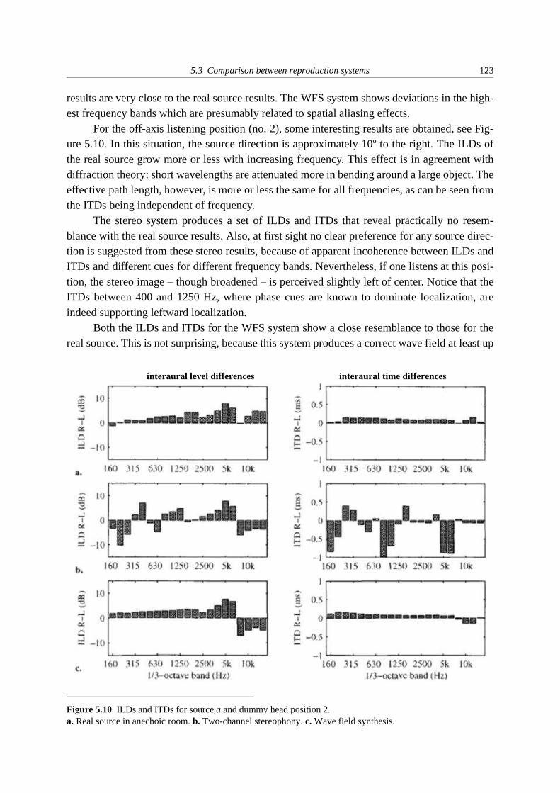
5.3 Comparison between reproduction systems 123
results are very close to the real source results. The WFS system shows deviations in the high-est frequency bands which are presumably related to spatial aliasing effects.
For the off-axis listening position (no. 2), some interesting results are obtained, see Fig-ure 5.10. In this situation, the source direction is approximately 10º to the right. The ILDs ofthe real source grow more or less with increasing frequency. This effect is in agreement withdiffraction theory: short wavelengths are attenuated more in bending around a large object. Theeffective path length, however, is more or less the same for all frequencies, as can be seen fromthe ITDs being independent of frequency.
The stereo system produces a set of ILDs and ITDs that reveal practically no resem-blance with the real source results. Also, at first sight no clear preference for any source direc-tion is suggested from these stereo results, because of apparent incoherence between ILDs andITDs and different cues for different frequency bands. Nevertheless, if one listens at this posi-tion, the stereo image – though broadened – is perceived slightly left of center. Notice that theITDs between 400 and 1250 Hz, where phase cues are known to dominate localization, areindeed supporting leftward localization.
Both the ILDs and ITDs for the WFS system show a close resemblance to those for thereal source. This is not surprising, because this system produces a correct wave field at least up
Figure 5.10 ILDs and ITDs for source a and dummy head position 2.a. Real source in anechoic room. b. Two-channel stereophony. c. Wave field synthesis.
interaural level differences interaural time differences

124 Chapter 5: Objective Evaluation
to the aliasing frequency of 1340 Hz (calculated from Equation (2.35) using ∆x = 12.7 cm). Inthis situation, the aliased waves appear not to affect the ILDs and ITDs below the 8 kHz-band.
For source b, the dummy head is again placed at the sweet spot position 1. The results areagain in favor of the WFS system, as shown in Figure 5.11. The stereo system, here using sig-nals recorded by the simulated-ORTF system* , produces fairly consistent responses. Its ITDscorrespond with that of a source nearly 30º to the left†, which indicates that the sound from theleft loudspeaker is decisive in this aspect. The high frequency ILDs support this phantomimage direction.
It can be concluded that the imaging capabilities of the reproduction systems can beunderstood reasonably well by examining the ITDs and ILDs in 1/3-octave bands. The methoddoes not claim to give the actual image source direction, but provides results that are consistentwith previously gained insight in stereophonic imaging and in wave fields created by WFS.
Concerning the results of the reproduction systems, this qualification technique suggestsa constant high quality image direction for the WFS system: for frequencies to about 5 kHz at
* The ORTF-pair gives 0.3 ms delay and 7 dB level difference between both stereo signals. † A source direction of 150º is also possible for these ITDs, but can be excluded here for obvious reasons.
Figure 5.11 ILDs and ITDs for source b and dummy head position 1.a. Real source in anechoic room. b. Two-channel stereophony. c. Wave field synthesis.
interaural level differences interaural time differences
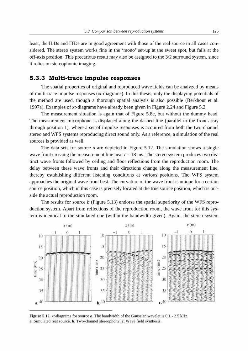
5.3 Comparison between reproduction systems 125
least, the ILDs and ITDs are in good agreement with those of the real source in all cases con-sidered. The stereo system works fine in the ‘mono’ set-up at the sweet spot, but fails at theoff-axis position. This precarious result may also be assigned to the 3/2 surround system, sinceit relies on stereophonic imaging.
5.3.3 Multi-trace impulse responses
The spatial properties of original and reproduced wave fields can be analyzed by meansof multi-trace impulse responses (xt-diagrams). In this thesis, only the displaying potentials ofthe method are used, though a thorough spatial analysis is also possible (Berkhout et al.1997a). Examples of xt-diagrams have already been given in Figure 2.24 and Figure 5.2.
The measurement situation is again that of Figure 5.8c, but without the dummy head.The measurement microphone is displaced along the dashed line (parallel to the front arraythrough position 1), where a set of impulse responses is acquired from both the two-channelstereo and WFS systems reproducing direct sound only. As a reference, a simulation of the realsources is provided as well.
The data sets for source a are depicted in Figure 5.12. The simulation shows a singlewave front crossing the measurement line near t = 18 ms. The stereo system produces two dis-tinct wave fronts followed by ceiling and floor reflections from the reproduction room. Thedelay between these wave fronts and their directions change along the measurement line,thereby establishing different listening conditions at various positions. The WFS systemapproaches the original wave front best. The curvature of the wave front is unique for a certainsource position, which in this case is precisely located at the true source position, which is out-side the actual reproduction room.
The results for source b (Figure 5.13) endorse the spatial superiority of the WFS repro-duction system. Apart from reflections of the reproduction room, the wave front for this sys-tem is identical to the simulated one (within the bandwidth given). Again, the stereo system
Figure 5.12 xt-diagrams for source a. The bandwidth of the Gaussian wavelet is 0.1 - 2.5 kHz. a. Simulated real source. b. Two-channel stereophony. c. Wave field synthesis.
b.a. c.

126 Chapter 5: Objective Evaluation
reproduces the simulated-ORTF signals, yielding two wave fronts rather than one: theresponses of both loudspeakers can be recognized immediately.
5.3.4 Intensity measurements
The sound intensity is a vector quantity defined as
, (5.3)
where p is the sound pressure and v is the particle velocity at r. The time-averaged sound inten-sity reads
, (5.4)
with T the period of averaging. The sound intensity can be interpreted as the power flux througha surface of unity area. For a monopole source, I is directed radially. This property is useful todetermine the source direction in a sound field: in absence of other sources and reflections, thesource is located in the direction opposite to that of I.
In a reflective environment, the intensity is a resultant of sound entering from all direc-tions. If sound waves are entering equally strong from all directions, e.g. in a reverberationchamber, the intensity approaches zero. Hence, a low value for | I | is a necessary condition indetermining whether a sound field is diffuse* . Since the sound intensity depends on thestrength of the source, a better condition of diffuseness can be derived from the reactivityindex, defined as the intensity level minus the sound pressure level:
Figure 5.13 xt-diagrams for source b. The bandwidth of the Gaussian wavelet is 0.1 - 2.5 kHz.a. Simulated real source. b. Two-channel stereophony. c. Wave field synthesis.
a. b. c.
I r t,( ) p r t,( ) v r t,( )=
Iav1T--- p t( )v t( ) td
0
T
∫=

5.3 Comparison between reproduction systems 127
. (5.5)
The reactivity index is zero for a source in the free field, and negative in a diffuse field.The sound intensity is measured on a grid in the reproduction room, as depicted in Figure
5.14a. The measurement probe (Figure 5.14b) consists of two calibrated pressure microphonesseparated by a 12 mm spacer. The probe is placed at a grid point, pointing in the x-direction.During 4 seconds of averaging, Ix,av is measured, after which the probe is rotated manuallytowards the z-direction. The intensity vector is calculated by composing Ix,av and Iz,av in thehorizontal plane (Figure 5.14c). The vertical component Iy,av is not measured. The accuracy ofmeasurement is guaranteed only in the frequency range between about 250 Hz and 5 kHz, dueto the finite-difference approximation used. All measurements presented here employ this fre-quency range.
* Note that | I | = 0 is not a sufficient condition: it only requires that sound waves entering from opposite direc-tions should cancel (e.g. two equal plane waves traveling in opposite directions yield | I | = 0, but are not dif-fuse). Caution is therefore needed in interpreting low values of sound intensity as a proof of diffuseness.
LK LI LP [dB]–=
Figure 5.14 a. Two sources a and b are imaged by each of the reproduction systems. Source c is imaged only bythe WFS system by means of focusing. Intensity measurements are carried out on a 7×9 grid. (Positions 1 to 3 referto sound pressure measurements of Section 5.3.5). b. The intensity probe (B&K 3545) determines the intensity atthe axis through both microphones. c. The intensity vector in the horizontal plane is composed of measurementsalong two perpendicular axes at each grid point.

128 Chapter 5: Objective Evaluation
The intensity distributions of direct sound, early reflections and reverberation are investi-gated separately for two-channel stereophony, 3/2 surround and WFS. The imaging techniquefor direct sound for the 3/2 system is purely stereophonic (‘2/0’), as in the previous section. Anextension towards 2/2 surround is used for early reflections and reverberation. So again, thecenter loudspeaker is not incorporated.
Direct sound
The results for the direct sound from source a are shown in Figure 5.15. The intensityvectors are drawn at each grid point. The length of an arrow is a measure for the intensity level,as indicated below each plot by the extrema measured. E.g. ‘76 dB (max)’ means that 76 dB isthe maximum value of | I | in this plot. Comparison of both reproduced intensity distributionswith the simulated distribution learns that the WFS system is closer to the ideal situation. Afew disturbances are probably caused by reflections in the reproduction room.
For source b in Figure 5.16, the distribution for the stereo system using the ORTF-pair isdominated by the left-hand loudspeaker, which produces a signal power that is 7 dB higherthan that of the right-hand one. The direction of the intensity vectors at the rear end of the lis-tening area is hardly influenced by this power difference. The results for the WFS system alsoshow deviations in the rear part of the listening area, though much smaller than those of thestereo system. These artefacts can be ascribed to the deactivation of the rear left-hand arraybar, which has been motivated by economical reasons (see Figure 4.15).
Instead of simulating real source c, the response of a loudspeaker at this position is mea-sured (Figure 5.17a). This source can only be reproduced by the WFS system. Not surprisingly,the direction of the intensity vectors in the area between focus and contributing arrays is oppo-
Figure 5.15 Intensity vectors for the direct sound of source a. Only the active loudspeakers and arrays are drawn.a. Simulated real source. b. Two-channel stereophony. c. Wave field synthesis.
a. b. c.

5.3 Comparison between reproduction systems 129
site to that of the real source. At the focus itself, the resultant intensity vector is directed awayfrom the contributing arrays. At some distance away from the focus, the vector field for theWFS system is similar to the ideal field.
Figure 5.16 Intensity vectors for the direct sound of source b. Only the active loudspeakers and arrays are drawn.a. Simulated real source. b. Two-channel stereophony. c. Wave field synthesis.
a. b. c.
Figure 5.17 Intensity vectors for the direct sound of source c. Only the active arrays are drawn.a. Real source (measured response of a loudspeaker at this position). b. Wave field synthesis.
a. b.

130 Chapter 5: Objective Evaluation
Early reflections
The early reflections of source b are modeled in the following manner. A simple virtualhall with a reasonable number of early lateral reflections is designed, see Figure 5.18. Thearrival times of the first twelve reflected waves (first and second order) vary between 20 and120 ms. The two-channel stereo system uses an ORTF-pair at the center (×) to image thesereflections. The 2/2 surround system employs an ORTF-quartet (see Figure 1.20b) at this posi-tion. The WFS system reproduces the reflections by means of virtual mirror sources.
In interpreting and comparing the energy flows, see Figure 5.19, some anomalies attractattention. The pattern for the stereo system is very similar to that for the monophonic situationof source a, shown in Figure 5.15b. Obviously, the temporal fine structure of the loudspeakersignals is lost in the results during averaging – only the total sound power remains, which ismore or less the same for both loudspeakers in this situation. These measurements confirm thelack of envelopment in stereophony: all sound power enters from the front.
The influence of the surround loudspeakers on the vector pattern is marginal, but clearlyvisible (Figure 5.19b). Indeed, the rear loudspeakers are radiating about 3 dB less energy thanthe front ones, for this particular hall model and ambient microphone technique. Most impor-tant however, is that lateral sound energy is missing in this configuration.
For the WFS system, the ‘flow’ of the intensity vectors can be understood by regardingthe concentrations of mirror sources around the arrays. The highest power is generated by bothvirtual mirror sources near the front left-hand corner, because they are closest to the listeningarea. Other groups of mirror sources assert their influence to a lesser degree. In this reproduc-tion method, the lateral reflections are truly incident from the sides.
Figure 5.18 Mirror sources (º) from source b (•) as a consequence of a large hall (thick lines). The rectangulararray configuration is drawn to the same scale. The absorption coefficient of the rear wall is 0.5, while it is 0.2 forthe other walls.
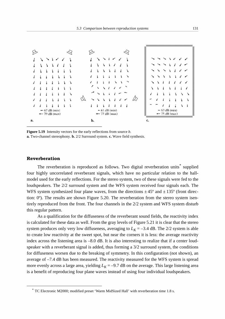
5.3 Comparison between reproduction systems 131
Reverberation
The reverberation is reproduced as follows. Two digital reverberation units* suppliedfour highly uncorrelated reverberant signals, which have no particular relation to the hall-model used for the early reflections. For the stereo system, two of these signals were fed to theloudspeakers. The 2/2 surround system and the WFS system received four signals each. TheWFS system synthesized four plane waves, from the directions ± 45º and ± 135º (front direc-tion: 0º). The results are shown Figure 5.20. The reverberation from the stereo system isen-tirely reproduced from the front. The four channels in the 2/2 system and WFS system disturbthis regular pattern.
As a qualification for the diffuseness of the reverberant sound fields, the reactivity indexis calculated for these data as well. From the gray levels of Figure 5.21 it is clear that the stereosystem produces only very low diffuseness, averaging to LK = –3.4 dB. The 2/2 system is ableto create low reactivity at the sweet spot, but near the corners it is less: the average reactivityindex across the listening area is –8.0 dB. It is also interesting to realize that if a center loud-speaker with a reverberant signal is added, thus forming a 3/2 surround system, the conditionsfor diffuseness worsen due to the breaking of symmetry. In this configuration (not shown), anaverage of –7.4 dB has been measured. The reactivity measured for the WFS system is spreadmore evenly across a large area, yielding LK = –9.7 dB on the average. This large listening areais a benefit of reproducing four plane waves instead of using four individual loudspeakers.
* TC Electronic M2000; modified preset ‘Warm MidSized Hall’ with reverberation time 1.8 s.
Figure 5.19 Intensity vectors for the early reflections from source b.a. Two-channel stereophony. b. 2/2 Surround system. c. Wave field synthesis.
a. b. c.
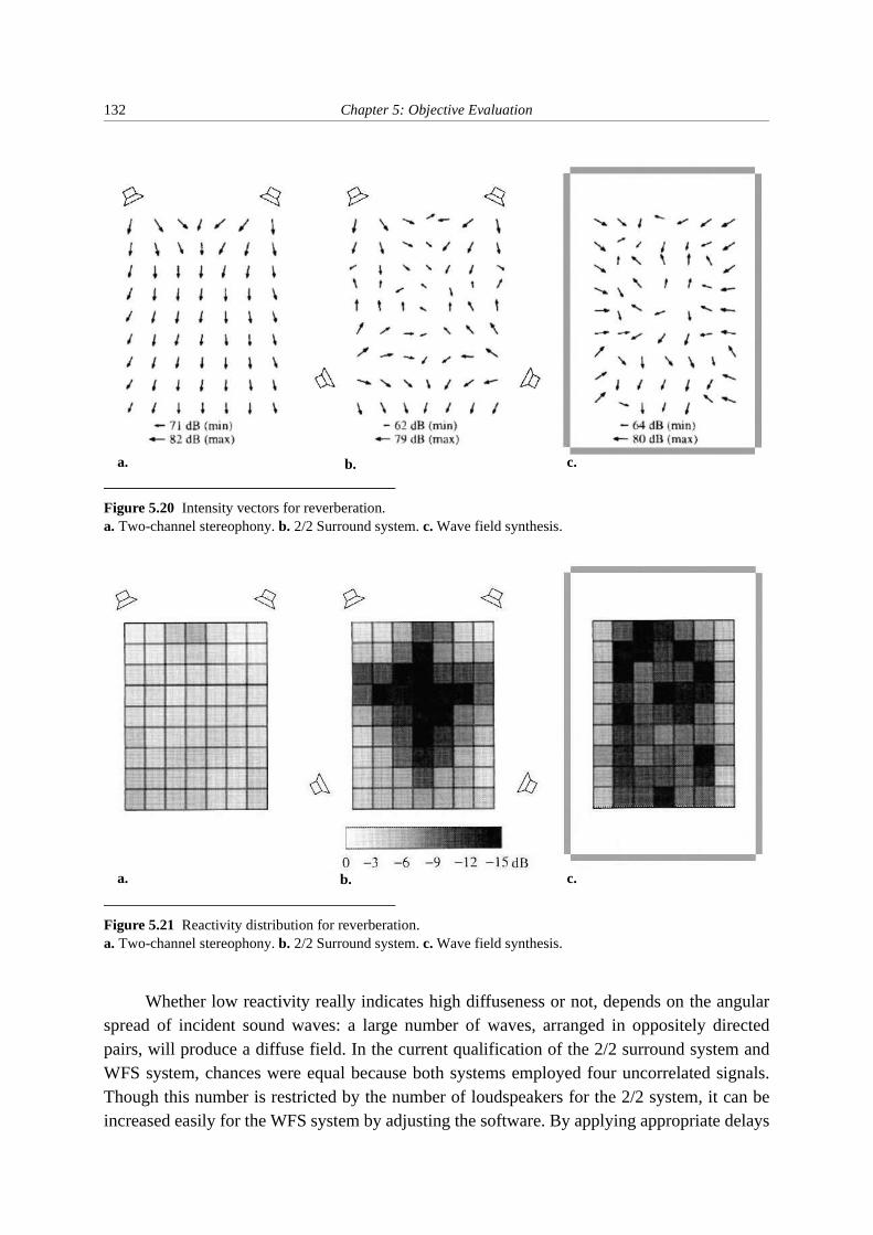
132 Chapter 5: Objective Evaluation
Whether low reactivity really indicates high diffuseness or not, depends on the angularspread of incident sound waves: a large number of waves, arranged in oppositely directedpairs, will produce a diffuse field. In the current qualification of the 2/2 surround system andWFS system, chances were equal because both systems employed four uncorrelated signals.Though this number is restricted by the number of loudspeakers for the 2/2 system, it can beincreased easily for the WFS system by adjusting the software. By applying appropriate delays
Figure 5.20 Intensity vectors for reverberation.a. Two-channel stereophony. b. 2/2 Surround system. c. Wave field synthesis.
a. b. c.
Figure 5.21 Reactivity distribution for reverberation.a. Two-channel stereophony. b. 2/2 Surround system. c. Wave field synthesis.
a. b. c.

5.3 Comparison between reproduction systems 133
to the available reverberant signals, a much higher number of perceptually uncorrelated wavescan be created. Maat (1997) found that with the present horizontal reproduction array, no morethan ten uncorrelated plane waves were necessary to create a perceptually diffuse sound fieldfor trained subjects. For less-trained subjects a lower number of plane waves sufficed.
5.3.5 Frequency spectrum measurements
Together with the intensity data of the previous section, the time-averaged sound pres-sure levels at the grid points have been collected in 1/3-octave bands. A selection of these datahas been made to illustrate some typical spectra for the reproduction of direct sound by two-channel stereophony and WFS. These typical responses are measured at three adjacent gridpoints close to the stereophonic sweet spot. The choice of the positions is based on the consid-eration that stereophonic reproduction suffers from comb-filter effects, which depend on thelistening position with respect to the sweet spot (Section 1.6.4). In anechoic circumstances,such dips can easily be perceived as coloration. In a reflective environment, the spectral distor-tion is usually masked by early reflections that arrive within the integration time of the audi-tory system. Though in the present measurements not only early, but also later arrivingreflections are included in averaging, the spectral influence of the latter can be neglected asthey possess much less strength. Therefore, the measured spectra can be regarded to be signifi-cant in determining whether there will be big differences in sound color perceived at thesepositions. It will be interesting to compare the differences for stereophony with those for theWFS system.
Figure 5.22 Frequency responses of the direct sound of source a, measured at positions 1 (thick line), 2 (dashedline) and 3 (thin line) as defined in Figure 5.14a. a. Two-channel stereophony. b. Wave field synthesis.

134 Chapter 5: Objective Evaluation
Figure 5.22 shows the 1/3-octave band spectra of the reproduced direct sound of sourcea, measured at the grid points marked 1, 2 and 3 in Figure 5.14a. Except for some bigger differ-ences at frequencies , the spread of the three spectra is within ± 2 dB for both repro-duction systems. For source b, see Figure 5.23, the spread of the responses is slightly larger (±3 dB), but again both reproduction methods produce comparable results. Similar observationswere made at many other grid points, which justifies the conclusion that the frequencyresponses of both systems, measured in 1/3-octave bands, are equally robust in a large listeningarea.
5.4 Conclusions
Frequency responses of virtual sources at different distances from the array have beenmeasured. The sound pressure levels of virtual sources at some distance from the arrays obeythe 1/r-law. However, close to the arrays (< 1 m) the 1/r-law does not hold due to the use of lin-ear arrays instead of planar arrays.
The effect of spatial aliasing for focused and non-focused virtual sources appear in dif-ferent regions of the synthesized wave field for each type of source. This result, that can beexplained in terms of wave field reconstruction, favors the frequency response of focusedsources near the central axis of its wave field. The sound pressure levels in the focal area reveal
500 Hz≤
Figure 5.23 Frequency responses of the direct sound of source b, measured at positions 1 (thick line), 2 (dashedline) and 3 (thin line) as defined in Figure 5.14a. a. Two-channel stereophony. b. Wave field synthesis.

5.4 Conclusions 135
a steep maximum along a line parallel to the array: a level difference of 18 dB is measuredbetween two positions 0.5 meter apart, which is in accordance with theory.
The wave field synthesis (WFS) system is compared with two-channel stereophony and3/2 surround sound. The image directions, as produced by these systems, are qualified by inter-preting the interaural time and sound pressure level differences measured at a dummy head. Asexpected, the results for stereophonic imaging depend on the listening position, in contrastwith the WFS system which creates a large listening area.
A second qualification technique, multi-trace impulse responses, illustrates the spatialproperties of the reproduced wave field. The WFS system produces wave fronts that are copiesof the original ones, while with stereophonic imaging the separate contributions of both loud-speakers remain.
This is confirmed by a third qualification technique: intensity vector measurements. Alsothe distribution of early reflections has been visualized by this technique. Though adding sur-round loudspeakers to two-channel stereophony already greatly progressed the imaging ofreflections, a clear lack of incident sound energy still remains to the sides. The advantage ofthe WFS system in this aspect is that sound can be reproduced from all around the listeningarea. This system also possesses the capabilities of creating a diffuse reverberant field in alarge listening area. With the 2/2 system, only a point solution is offered, while two-channelstereophony cannot generate a diffuse field at all.
Finally, the sound pressure levels of reproduced direct sound have been collected in 1/3-octave bands. The spectra for stereophony and WFS do not depend strongly on the position ofmeasurement. The 1/3-octave band spectra for both systems are of comparable smoothness.

136 Chapter 5: Objective Evaluation

137
Chapter 6
Subjective Evaluation
6.1 Introduction
The imaging capabilities of wave field synthesis are investigated perceptually in twoways: by localization experiments of virtual sources, and by a listening test in which wavefield synthesis is compared directly to two-channel stereophony and 3/2 surround sound.Through localization experiments it is attempted to prove that wave field synthesis is able toreproduce sources at correct positions. The comparative listening tests were carried out to indi-cate roughly whether the newly-built system is superior to the other systems concerningrobustness, flexibility and quality.
6.2 Localization experiments
The localization of virtual sources was compared to the localization of real sources intwo sessions of subjective listening tests. The first session (A) investigated the localization ofvirtual sources behind the loudspeaker array, while the second session (B) dealt with virtualsources in front of the array. In these experiments, only directional hearing in the horizontalplane was considered. The array consisted of 24 custom-built electrodynamic loudspeakers(Vifa M-110 4" drivers with ∆x = 11 cm) described by Vogel (1993) — the new reproductionsystem was not available yet at the time of these experiments.
A map of the situation is drawn in Figure 6.1. The listener was seated at a distance of 3 mfrom the array (with numbered loudspeakers), and was free to move his head. The virtual

138 Chapter 6: Subjective Evaluation
sources were synthesized either at 2 m behind the array or at 1 m in front of the array. The realsources were produced by single array loudspeakers. Five dummy loudspeakers wereappended to either side of the array to avoid bias by limited choice. In this way, the angularspacing of the loudspeakers varied from 1.6º at the edges to 2.1º in the middle of the array.
Basically, the set-up and data processing method for this source-identification experi-ment is taken from Hartmann (1983). He investigated the influence of room reflections on thelocalization of sound sources with the aid of eight loudspeakers placed 4º apart at 12 m fromthe subject. The results can be described by at least three important statistical quantities. If M isthe number of trials per source, Si the stimulus direction and Ri the response direction for triali, then the rms error for source k is defined as
. (6.1a)
The mean response of a certain subject for source k is given by
. (6.1b)
The standard deviation for source k equals
1 2 3 ... ... 34
xz
z = 0
z = 1
z = –2
z = 3
virtual sourcesexp. B
virtual sourcesexp. A
20º
real sourcesexp. A and B
(0,0)
Figure 6.1 Situation map for both of the localization experiments. The origin of the coordinate system is at themiddle of the array. The 20º azimuth is relevant for the understanding of effective aperture effects as explained inthe text.
array
D k( ) Ri k( ) Si k( )–( )2M⁄
i∑ 1 2⁄
=
R k( ) Ri k( ) M⁄i∑=

6.2 Localization experiments 139
. (6.1c)
It can be meaningful to average D(k) and s(k) across sources k. Then, these quantities are writtenas D and s, respectively. Statistic quantities averaged across subjects are notated as <...>.
Because the tested parameters differed between both experiments, their set-up isdescribed in more detail in separate sections.
6.2.1 Virtual sources behind the array (exp. A)
Environment
The test series were carried out in an anechoic room, and repeated in the reproductionroom (Section 4.3.2). In the latter room, the z-axis of Figure 6.1 was parallel to the side walls.The array was placed about 1.5 m from the front wall, and directed toward the rear wall.
Stimuli
Frozen white noise bursts with a duration of 1500 ms were used as stimuli. Attack tran-sients were avoided by rise and decay durations of 15 ms. After each stimulus there was apause of 5 seconds. The input signals were compensated for the average on-axis response ofthe loudspeakers (similar as mentioned in Section 4.3.4), resulting in a nearly flat spectrum inthe range from 100 Hz to 16 kHz. The array was tapered with a cosine-window over the outer3 loudspeakers, in order to diminish truncation effects.
Variables
Position of the virtual source. There were 13 fixed virtual source positions at a distanceof 2 m behind the array, ranging from x = –3 m to x = 3 m in steps of 0.5 m. The outer positionswere expected to be difficult to localize because the subject’s position was outside the recon-struction area for these virtual sources (as defined in Figure 2.18).
The spacing ∆x of the loudspeakers. Two spacings of the loudspeakers were programed:∆x = 11 cm and ∆x = 22 cm. The latter was obtained by addressing alternating speakers, leav-ing the total array length unchanged.
These parameters were varied during one experimental run. There were two trials persource direction. In a separate run, also six real sources were presented. The subjects were notinformed of the special nature of this run. Ten subjects participated, all males aged 20 to 30years without hearing complaints.
Task
The subjects were asked to estimate the direction of the sound by writing down the num-ber of the loudspeaker closest to that direction.
s k( ) Ri k( ) R k( )–[ ]2 M⁄i∑ 1 2⁄
=
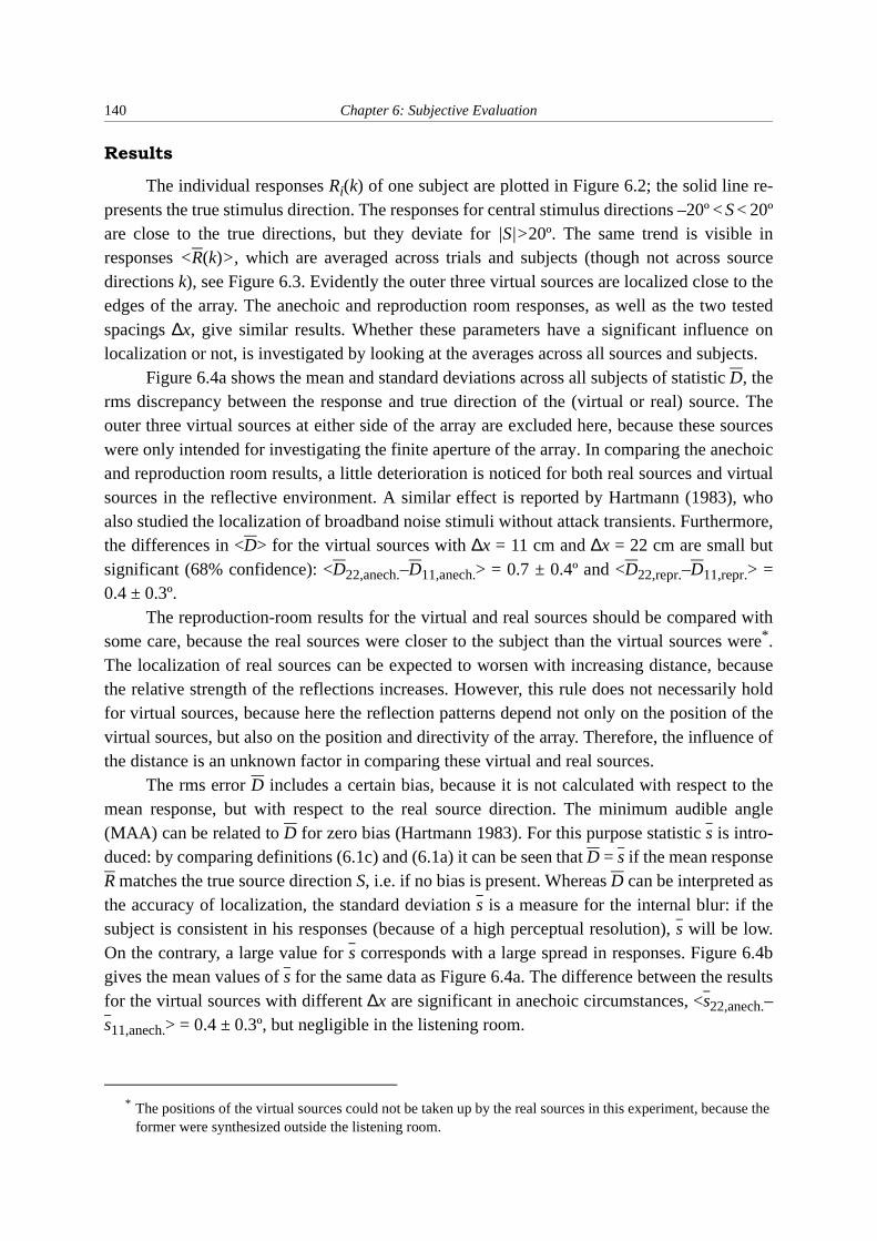
140 Chapter 6: Subjective Evaluation
Results
The individual responses Ri(k) of one subject are plotted in Figure 6.2; the solid line re-presents the true stimulus direction. The responses for central stimulus directions –20º < S < 20ºare close to the true directions, but they deviate for |S|>20º. The same trend is visible inresponses <R(k)>, which are averaged across trials and subjects (though not across sourcedirections k), see Figure 6.3. Evidently the outer three virtual sources are localized close to theedges of the array. The anechoic and reproduction room responses, as well as the two testedspacings ∆x, give similar results. Whether these parameters have a significant influence onlocalization or not, is investigated by looking at the averages across all sources and subjects.
Figure 6.4a shows the mean and standard deviations across all subjects of statistic D, therms discrepancy between the response and true direction of the (virtual or real) source. Theouter three virtual sources at either side of the array are excluded here, because these sourceswere only intended for investigating the finite aperture of the array. In comparing the anechoicand reproduction room results, a little deterioration is noticed for both real sources and virtualsources in the reflective environment. A similar effect is reported by Hartmann (1983), whoalso studied the localization of broadband noise stimuli without attack transients. Furthermore,the differences in <D> for the virtual sources with ∆x = 11 cm and ∆x = 22 cm are small butsignificant (68% confidence): <D22,anech.–D11,anech.> = 0.7 ± 0.4º and <D22,repr.–D11,repr.> =0.4 ± 0.3º.
The reproduction-room results for the virtual and real sources should be compared withsome care, because the real sources were closer to the subject than the virtual sources were* .The localization of real sources can be expected to worsen with increasing distance, becausethe relative strength of the reflections increases. However, this rule does not necessarily holdfor virtual sources, because here the reflection patterns depend not only on the position of thevirtual sources, but also on the position and directivity of the array. Therefore, the influence ofthe distance is an unknown factor in comparing these virtual and real sources.
The rms error D includes a certain bias, because it is not calculated with respect to themean response, but with respect to the real source direction. The minimum audible angle(MAA) can be related to D for zero bias (Hartmann 1983). For this purpose statistic s is intro-duced: by comparing definitions (6.1c) and (6.1a) it can be seen that D = s if the mean responseR matches the true source direction S, i.e. if no bias is present. Whereas D can be interpreted asthe accuracy of localization, the standard deviation s is a measure for the internal blur: if thesubject is consistent in his responses (because of a high perceptual resolution), s will be low.On the contrary, a large value for s corresponds with a large spread in responses. Figure 6.4bgives the mean values of s for the same data as Figure 6.4a. The difference between the resultsfor the virtual sources with different ∆x are significant in anechoic circumstances, <s22,anech.–s11,anech.> = 0.4 ± 0.3º, but negligible in the listening room.
* The positions of the virtual sources could not be taken up by the real sources in this experiment, because the former were synthesized outside the listening room.
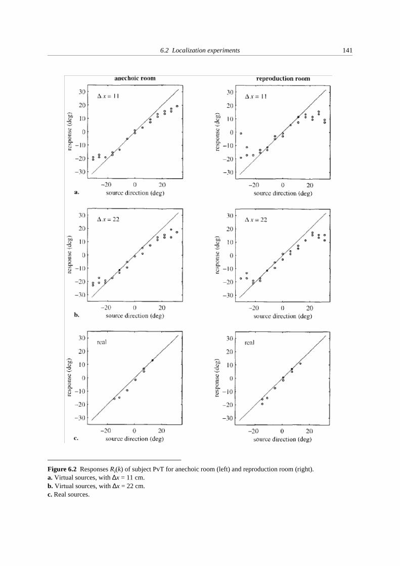
6.2 Localization experiments 141
Figure 6.2 Responses Ri(k) of subject PvT for anechoic room (left) and reproduction room (right). a. Virtual sources, with ∆x = 11 cm.b. Virtual sources, with ∆x = 22 cm.c. Real sources.

142 Chapter 6: Subjective Evaluation
Figure 6.3 Mean responses <R(k)> across all trials and subjects for anechoic room (left) and reproduction room(right). The error bars are have a width of twice <s(k)>.a. Virtual sources, with ∆x = 11 cm.b. Virtual sources, with ∆x = 22 cm.c. Real sources.

6.2 Localization experiments 143
Discussion
The bending of the response curve in Figures 6.2 and 6.3 for azimuths greater than 20ºgives rise to a rule in wave field synthesis, stating that no source can be localized in a directionwere no loudspeaker is active. In other words, the listener perceives the space of virtualsources through an acoustic window: the array. This space is restricted by two lines of sightfrom the listener to positions near the edges of the array (dashed lines in Figure 6.1).
Start (1997) was able to compare the standard deviation <s> and the MAA measured forvirtual sources, by re-analyzing similar source-identification experiments from Vogel (1993)and using his own results for the MAA. Since Vogel did not apply the spacing ∆x = 22 cm nordid he use real sources, only a comparison of the virtual source results for ∆x = 11 cm was pos-sible. The present work completes this comparison of anechoic results, shown in Table 6.1.
Table 6.1 Comparison of localization experiments in anechoic circumstances.
<s> (Verheijen) MAA (Start) <s> (Vogel)
real sources 0.96 ± 0.18º 0.79 ± 0.09º
virtual sources; ∆x = 11 cm 0.94 ± 0.10º 0.77 ± 0.11º 1.1 ± 0.1º
virtual sources; ∆x = 22 cm 1.37 ± 0.29º 1.57 ± 0.23º
stimulus type white noise white noise pink noise
bandwidth 0.1 to 16 kHz 0.1 to 8 kHz 0.1 to 8 kHz
subjects × trials 10×14 3×300 3×60
array length 2.7 m 5.4 m 5.4 m
experiment in situ KEMAR recordings in situ
Figure 6.4 Mean results across sources and subjects, for virtual sources (∆x = 11 and ∆x = 22 cm) and real sources.a. Mean rms error <D>.b. Mean standard deviation <s>.
<D
> (
deg
)
anechoic room reproduction room
<s>
(d
eg)
anechoic room reproduction room
11 real22 11 real22 11 real22 11 real22
a. b.

144 Chapter 6: Subjective Evaluation
The results support the arguments of Hartmann (1983) that the value for the MAA andthe value for <s> are of the same order. In addition, it can be concluded that an increased spac-ing between the loudspeakers causes an increased localization blur. There is no significant dif-ference in localization blur between real sources and virtual sources with ∆x = 11 cm.
6.2.2 Virtual sources in front of the array (exp. B)
Environment
The test series were carried out in an anechoic room only.
Stimuli
Random pink noise bursts with a duration of 2 seconds were used as stimuli. The abruptedges of the stimuli provided additional localization cues. It was considered that in their local-ization properties, such stimuli are closer to speech and (rhythmic) music than are cosine-win-dowed stimuli. A pause of 2 seconds followed each stimulus. Due to hardware limitations, thecorrection factor from driving function (2.29b) was not implemented here, whichemphasizes the low frequencies. The array was tapered over the outer 4 loudspeakers with acosine-window to diminish truncation effects. A cut-off filter at 16 kHz limited the bandwidth.
Variables
Position of the virtual source. There were 25 fixed virtual source positions at a distanceof 1 m in front of the array, at azimuthal intervals of 2º. The outer virtual sources wereexpected to be difficult to localize, because they are influenced by array truncation effects.
The bandwidth of the stimulus. The aliased waves of focused sources travel ahead of theactual wave fronts. The aliased waves that arrive earliest are radiated from the outermost arrayelements (see Figure 5.4b). It was expected that erroneous localization would appear, if onlyfrequencies above the aliasing frequency were produced. To investigate this, the experimentwas repeated with high-pass filtered stimuli (2 – 16 kHz).
Position of the subject. Besides the base position at (x, z) = (0, 3), see Figure 6.1, also aposition at (–1, 3) was used. Here, only the broadband virtual sources were presented.
In one run, each virtual source was presented four times at random. Two subjects partici-pated, doing each run twice, thus yielding eight trials per source. In a separate run at the baseposition, also 24 real sources (the array loudspeakers) were produced, with both broadbandand high-pass filtered signals.
Task
The subjects were asked to estimate the direction of the sound by writing down the num-ber of the loudspeaker closest to that direction.
k j⁄

6.2 Localization experiments 145
Results and discussion
The individual responses R(k) of both subjects are depicted in Figure 6.5; the solid linerepresents the true direction. For the virtual sources, a localization aperture seems to be ineffect for about | S | < 18º. This is a bit less than the aperture in exp. A, which is probably aresult of the wider taper applied in this experiment. Also, a clear bias for virtual as well as forreal sources is present in the results of subject GJ. The results for the high-pass filtered stimulido not deviate significantly from the broadband results. Apparently, the localization task is nothindered by the (first-arriving) aliased waves from the outer loudspeakers. Because the densealiasing tail does not exceed a few milliseconds, an integration mechanism in the auditory sys-tem may be held responsible for the reasonable accuracy of localization for these focusedsources. The response function for the virtual sources is, however, not as regular as for the realsources. This regularity can be expressed by the linear correlation coefficient r, being betterthan 0.999 for the real sources and ranging from 0.991 to 0.993 for the virtual sources (withinthe aperture).
The responses for the listening position at (–1, 3) are shown in Figure 6.6. At this posi-tion, the outermost active loudspeaker is at 38º, while the bending of the response functionstarts already at about 30º. Like for virtual sources behind the array, the effective acoustic win-dow is smaller than the array width.
Figure 6.7 summarizes the statistical parameters of the experiment (only for the baseposition of the subject). The differences in rms discrepancy D and response standard deviations between virtual and real sources are significant in all cases considered. However, a localiza-tion accuracy of less than 5º and a localization blur of less than 2º is still a good result for thevirtual sources.
6.2.3 Evaluation of both experiments
Due to the large bias for one of both subjects in experiment B, it is awkward to compare<D> for sources behind (exp. A) and in front of (exp. B) the arrays. The result of <s> for realsources, however, is approximately equal in both experiment sessions. Therefore it is alsoallowed to compare the results of <s> for the broadband virtual sources synthesized at eitherside of the array (Table 6.2), though some reserve is in order here because of the small numberof subjects in exp. B. The response standard deviation for focused virtual sources is about 80%greater than for non-focused sources. In an absolute sense, however, there is less differencethan 1º.
Table 6.2 Comparison of response standard deviation between experiment A and B.
< s > exp. A exp. B
real sources (º) 0.96 ± 0.18 1.08 ± 0.08
virtual sources (º) 0.94 ± 0.10 1.71 ± 0.08

146 Chapter 6: Subjective Evaluation
Figure 6.5 a. Responses R(k) for virtual sources with broadband stimuli.b. Responses for virtual sources with highpass-filtered (> 2 kHz) stimuli.c. Responses for real sources with broadband stimuli.

6.2 Localization experiments 147
6.2.4 Distance perception
Besides the direction of the source, the apparent distance of the source is also an impor-tant factor in sound reproduction. In contrast with directional hearing, depth perception is a rel-ative sensation with many sources active at the same time. In case of the absence of othersources, the perceived distance depends largely on the loudness of the source, but also on thesubject’s familiarity with the source signal (Blauert 1983). The distance control of virtualsources in the wave field synthesis system, as incorporated in the synthesis operator (Section5.2.2), is therefore not the only significant factor in distance judgements. Moreover, the dis-tance resolution of the human auditory system is rather poor. This is confirmed by subjectiveexperiments of Start et. al. (1997), who evaluated the distance perception of real and virtualsources in an auditorium. The subjects, seated 25 m from stage, were asked to judge the depth
Figure 6.6 Virtual source responses R(k) with broadband stimuli for the off-center listening position (x, z) = (–1,3).
Figure 6.7 a. The mean rms error D for virtual (gray bars) and real sources (white bars). b. The mean standard deviation s for virtual and real sources.
subject EV subject EVsubject GJ subject GJ
broad-
s (d
eg)
D (
deg
)
a. b.band
broad-
band
broad-
band
broad-
band>2 kHz >2 kHz >2 kHz >2 kHz

148 Chapter 6: Subjective Evaluation
level of the sources out of three possible depth levels, 2 m apart. For the real sources, 49% ofthe responses was correct, while for the virtual sources (behind an array installed at 15 m fromthe subjects) only 40% of the responses was correct. Both results are not impressively accu-rate, though they are above chance (33%).
For sources closer than about 1 m to the subject, the spectral influence of the headbecomes an important cue for distance estimations. Experiments of Komiyama et al. (1992)suggest that focused sources provide these cues very well. A planar array, consisting of loud-speakers arranged in concentric circles, was used to create focal points on the axis perpendicu-lar to the array, by applying ‘appropriate delay times’ to the loudspeaker signals in each circle.The experimental set-up was assessed empirically – no mathematical background is given. Thepurpose of the experiments was to find out whether the apparent distance of the sound imagescan be controlled with this array configuration. The results of their subjective experimentsshowed that a stable image can be localized near the focal point, even if the sound level of thefocused source was less than that of a reference loudspeaker at the same distance as the focus.
With a linear loudspeaker array instead of a planar array, the geometrical properties ofthe wave field are different. In informal tests with the laboratory demonstration system itappeared that the spectral cues of focused sources are less pronounced than those of realsources. However, if the listener is allowed to walk towards the focused source, a sense ofpresence is clearly felt. During many demonstrations with unexperienced as well as experi-enced listeners, with a saxophone recording being played back as a focused source, the listen-ers found the focus effortlessly. The feature of placing a soloist in front of the array is alsoutilized in one of the programs that serve as test material in the next section.
6.3 Comparison between reproduction systems
In this section, an attempt is made to qualify the laboratory wave field synthesis (WFS)system subjectively in comparison to two-channel stereophony and 3/2 surround sound. Theprevious chapter already investigated the shape of the wave fronts, reflective energy distribu-tion, reactivity index and frequency characteristics of these reproduction systems. The purposeof the tests in this section is to find subjective differences that are related to the reproductionmethod used by these systems.
6.3.1 Introduction
The difficulty in judging different sound reproduction systems is how to set up a test inwhich only properties of the system’s concept are compared. The influence of program mate-rial, the way of recording and mixing, differences in system hardware (loudspeakers, ADCs,etc.) and the placement of loudspeakers must evidently be minimized. In spite of all effort doneto set up a fair comparison, it should be realized that the results will certainly be biased byunwanted side-effects. Therefore, only large and obvious differences can be revealed by such atest.

6.3 Comparison between reproduction systems 149
Instead of regarding many subjective criteria separately, only three global criteria areconsidered:
1. Flexibility is a system property that allows the user to control the image.
2. Robustness refers to the stability of the image as experienced at different locations in thelistening area.
3. Quality is a global indication that refers to the spaciousness and naturalness of the image.
The criterion of flexibility is added because it is a novelty of the WFS system made pos-sible by its need of the bare microphone channels as inputs (Figure 4.3). Since stereo and 3/2surround systems receive and playback the downmix directly, it is awkward to demonstratethis property for these systems.
6.3.2 Experimental set-up
Listening panel
It is reasoned that for this comparison a relatively small number of subjects suffices, pro-vided that they agree unanimously on their findings. Preferably, the subjects must be able todiscriminate between concept-related and program-related differences in test material. Thisrequires a group of experienced listeners who are acquainted with each of the reproductionsystems under investigation. Therefore, the board that discussed the results of this researchproject twice a year, was invited for the test. Except the secretary, all of them were profession-ally involved in sound reproduction and/or acoustics. Those members of the board that wereconnected to the research group, were excluded from judgements. The participants were:
• a conservatory lecturer of recording engineering;
• a senior recording engineer of a record company;
• a consumer (the secretary of the board);
• a professor of perceptual acoustics;
• two acoustic researchers of a multinational electronics company.
Except the senior recording engineer, all had listened to the WFS system before. Four of themare professionally involved in 3/2 surround. All members are experienced stereo listeners.
Program material
Four music programs with a large difference in musical expression were selected (seealso Appendix B):
I. Violin concert in E Minor of Mendelssohn, first 10 minutes;
II. Second Symphony of Mahler, first 4 minutes of the first movement;
III. Conception of George Shearing (jazz), 5 minutes;
IV. Overture of the Concert after Vivaldi; arranged for saxophones, 3 minutes.

150 Chapter 6: Subjective Evaluation
The multi-track tapes of these unreleased recordings were mixed for each of the repro-duction systems by a graduate student who gained several years of experience in stereophonicmixing for a broadcasting corporation. His acquaintance with the 3/2 and WFS system wasmuch less, but after intensive practicing a fair level was obtained. His task was to strive for asound image that was virtually the same for each system, without favoring one above the other.The equalizers on the mixing console were not used. The mixed material was taped on a digitalmulti-track recorder in such a way that it could be reproduced synchronously for each system.The number of channels of the downmix was two for stereophony, five for 3/2 surround andeight for WFS (four virtual sources and four plane waves). The employed bandwidth is 22 kHzfor stereo and 3/2 surround, and 16 kHz for the WFS system. Documentation of the recordingand mixing sessions is provided in Appendix B.
The position of all loudspeakers during mixing and testing is depicted in Figure 5.7. Therear channels of the 3/2 downmix were delayed 2 ms to account for the smaller distance of therear loudspeakers to the sweet spot. The experimenter, standing in the rear right-hand cornernext to the mixing console, was able to switch directly between the reproduction systems.
Test procedure
Before entering the reproduction room, the participants received a short instruction toinform them of the test procedure and criteria of judgement. The participants attended the testtogether, but were urged not to talk during the tests. They were encouraged to walk about thelistening room, though not to approach the loudspeakers closer than 0.5 m. The music pro-grams were reproduced in the order shown above. The first piece of music was played twice.During the first play, the listeners could become familiar with all audible differences betweenthe three reproduction systems. After that, the experimenter switched at will between each sys-tem, thereby calling the name of the system that was just activated.
The experimenter demonstrated the flexibility of the WFS system by changing thesource positions and the ambience of program IV in a second play. Initially, the sources weremoved far-away from their original positions, while the reverberation lasted. After that, thefour sources were focused just in front of the corners of the array and the reverberant signalswere turned off, leaving a ‘dry’ atmosphere.
The participants were asked to write down their findings in a table. These quickly writtennotes served as an aid of memory for the actual evaluation that took place in a meeting roomimmediately after the test. There, the participants were asked one by one to comment on theperformance of the reproduction systems.
6.3.3 EvaluationConsensus was found among the participants on the following topics:
Coloration
Though coloration was not a criterion by itself, several participants responded spontane-ously that the differences in coloration between the systems were clearly audible, especially

6.3 Comparison between reproduction systems 151
between WFS on the one hand and both stereo and 3/2 surround on the other. Probably, thesedifferences are caused by the different type of loudspeakers used for WFS. Presumably alsospatial aliasing plays a role in the coloration heard for the WFS system. It is noted that boththese causes are hardware-related*. Nevertheless, it was agreed that the coloration differencesdid not obstruct a comparison based on the criteria listed hereafter.
Flexibility
The demonstrated flexibility of the WFS system (program IV) is appreciated as ‘obvi-ous’ and ‘beautiful’. It is considered that the feature of repositioning sources and changingacoustics is not only an important tool in post-production mixing, but also very interesting fornon-professional users.
Robustness
On the average, sources reproduced by the WFS system are found stabler than thosereproduced with 3/2 surround. The stereo image is the least robust. An exception to this rule isthe Mahler concert (II), in which some instruments are less stable in WFS as perceived at thesides. In program IV, the WFS system was far more robust than the others.
Quality
The WFS system reproduces an image with much more depth than the other systems do.Generally, also the spatial impression created by this system is appreciated above that ofothers. Especially the live atmosphere (rumble and audience noise) just before the start of theviolin concert (I) and the applause after the jazz song (III) is considered very convincing. How-ever, the symphony orchestras (I and II) appear to be a bit detached in WFS. This feeling ofdistance is probably due to the mixing of the orchestral program material, because, on the con-trary, the image of the jazz vocalist (III) seems to be almost touchable in WFS. This may becaused by the fact that her image is placed in front of the arrays: while approaching this image,its sound level increases in a realistic manner. The image of the saxophones (IV) in WFS isalso unequaled in naturalness by the other systems.
Many additional comments were reported, but most of these can be ascribed to personalpreference concerning ambience, depth and balance. Refining the mix would probably satisfysome of the respondents, but it would again dissatisfy others. Consensus was only reached onthe opinions reported above.
Some of the other comments are mentioned here to illustrate the spread in personalappreciation or professional approach of the respondents. Both recording engineers criticizedthe strength of the spot microphone signals, of which the prominent use is held responsible fora ‘double ambience’, in some programs of the stereo and WFS system. One of them disap-proved of the ‘over-acoustical detachment’ of WFS in the orchestral programs (I and II); the
* High quality array elements with higher directivity (Section 3.3) are proposed for reduction of coloration.
152 Chapter 6: Subjective Evaluation
other admired the natural sound of the WFS system: ‘You can’t hear the loudspeakers anymore.’ The latter also criticizes most of the 3/2 surround mixes, in which ‘the center channel isconfusing the image too much’. Other respondents did not share this opinion.
Discussion
For the Mahler program (II), the stability of the WFS sources is appreciated better in themiddle than at the sides of the listening area. This is caused by the conflicting use of spot andmain microphone signals. The spot microphones signals are fed to a limited number of virtualsources, while the main microphones signals, that also contain the direct sound of the spottedsources, are fed to virtual loudspeakers. In the middle of the listening area, the evoked imagescoincide, but at the sides the virtual stereo image collapses, while the virtual sources persist.Though the use of the main microphones signals does not provide an optimal reproductionquality here, it permits a considerable reduction of source signals and transmission channels.
A much better performance is obtained with the saxophone quartet (IV). Because of thesmall number of sources, each source could be recorded separately. The crosstalk was keptwithin bounds by minimizing the distance of the spot microphones to the sources. The ambientwaves from the front direction were provided by highly uncorrelated signals with a smalldirect/reverberation ratio. In this way, the possible conflicting images were avoided.
6.4 Conclusions
The localization experiments confirm that the localization of virtual sources behind thearray is as good as the localization of real sources. If the loudspeaker spacing of the arrays isdoubled to 22 cm, or if sources are focused in front of the arrays, a deterioration is observed,but the distortion is still small in an absolute sense. The localization blur for virtual sources isof the same order of magnitude as that for real sources.
From a subjective comparison of two-channel stereophony, 3/2 surround sound and wavefield synthesis, it appears that the wave field synthesis system is able to create a spatial impres-sion that is appreciated above that of the others. Also, the flexibility of placing sources andchanging ambience in this system is considered very positive. The wave field synthesis systemis more robust than the other systems, especially if crosstalk is minimized during recording.
While stereophonic recording can appeal to fifty years of experience, the development ofrecording for wave field synthesis has only just begun. Major improvements can be expectedfrom microphone and signal processing techniques that are able to decompose sound fieldsinto direct sound, reflections and reverberation. This will greatly benefit the flexibility andquality of sound reproduction.


161
Author Index
A
Ando 120
B
Bamford 25, 26, 118Bareham 118Barron 8Bartlett 16, 18, 21Bennett 12Beranek 4, 65, 66, 70, 81Berkhout 2, 4, 31, 32, 37, 45, 72, 95, 125Blake 27Blauert 7, 12, 16, 97, 147Bleistein 38Blumlein 1, 18Boer, De 1Boone 99, 119Bracewell 100Bradley 8, 99Burkhard 122Butterworth 1
C
Camras 1, 91Ceoen 21Clark 12, 19
Cooper 2, 25
D
Dalenbäck 92Damaske 118Dressler 24
E
Eargle 2, 24
G
Geluk 99Gerzon 24, 25, 26Griesinger 28
H
Hartmann 7, 138, 140, 144Hunt 1, 64, 67
I
ITU-R 28
J
Jansen 109
162 Author Index
K
Kate, Ten 23Komiyama 148
L
Lipshitz 16, 25
M
Maat 133Mac Cabe 118Macpherson 121Massa 1
P
Pierce 45, 50Potter 8, 82
R
Raatgever 121Reijnen 62Rife 4
S
Schneider 28Scholtze 122Skudrzyk 32Snow 1, 91Spikofski 28Start 37, 48, 62, 82, 88, 143, 147Steinberg 1Stern 121Streicher 18
T
Theile 28, 96, 122, 159Thorbecke 45Tohyama 118
V
Vogel 37, 52, 62, 82, 137, 143Vries, De 37, 50, 52
W
Watkinson 58Wightman 8, 82Willems 104Wöhr 158
Z
Zieglmeier 28

163
Subject Index
Numerics1/r-law 372D, abbr. of two dimensional3/2 system 283D, abbr. of three dimensional5.1 format 277.1 format 27
AAB, see Pairacoustic window 143ADC 58ambisonics 25apparent source width 8applications 62, 110array 63
design 78electrodynamic 79electrostatic 83two-way 79
Bbidirectional 18binaural 22
Ccanonical equations 64cardioid 18compatibility 11, 24, 25, 99compliance 66control unit 104convolution 5cross-correlation 120
DdB 4diaphragm shaping 73diffraction 7, 50diffuse 8, 126direct/reverberation ratio 20directivity 69
characteristic 37function 70pattern 18
discretization 54Disney 27distance perception 8, 147Dolby
B noise reduction 25Pro Logic 25Stereo 27

164 Subject Index
Surround 24driving function 48Duran Audio 101
Eearly reflections 8Edison 1equation of motion 33
Ffar-field approximation 37, 72filter
anti-aliasing 58comb 22IIR- 105kx- 60, 73
finite aperture 50, 140flexibility 149Fourier transform 5
double 56spatial 72
Fraunhofer area 72
GGaussian pulse 41geometrical parameters 94, 97
HHRTF 23Huygens iii
IIACC 118ILD 7, 120impedance 65impulse response 4ITD 7, 120
KKEMAR 122Kirchhoff-Helmholtz 32kxk-diagram 57
Llaw of sines 12localization 7
accuracy 140blur 7, 140
loudspeakerelectrodynamic 64electrostatic 67spacing 82subwoofers 104virtual 99volume 81
MMAA 140, 143mass 65matrix system 23microphone
ambient 96array 56, 60close miking 10main 20pressure 18SoundField 96spot 20, 93techniques 18velocity 18
monochromatic 44
NNyquist frequency 58
spatial 60
Oomnidirectional 18ORTF, see Pair
Ppair
AB 19Blumlein 18, 19ORTF 21, 29spaced 21XY 19

Subject Index 165
pan pot 20phonograph 1plane wave decomposition 56playback 97
Qquadraphony 23quality 149quality factor 66
RRayleigh I integral 34Rayleigh II integral 36reactivity index 127reconstruction area 50recording method 93reference line 41, 107reproduction room 103requirements for sound reproduction 9resonance frequency 66reverberation 8
time 4rhombic 74robustness 149
Ssampling
spatial 58temporal 59
Sommerfeld condition 34sound 3
engineer 2intensity 126
sourcefocused 45, 116mirror 98moving 95, 97, 99, 109notional 95phantom 11primary 33secondary 33signal 3static 106virtual 54
spaciousness 8
spatialaliasing frequency 60convolution 75
SPL 4stationary phase method 38, 40stereophony 10
intensity 1, 11time-based 16
sweet spot 10synthesis
operator 93, 101software 106
Ttapering 52transducer 1, 64transmission 24, 97truncation 50
Vvirtual reality 111voice coil 65volume velocity source 66
Wwave field synthesis 2, 31WFS, abbr. of wave field synthesis
Xxt-diagram 57XY, see Pairxz-diagram 57

166 Subject Index

167
References
Ando, Y. (1985), Concert Hall Acoustics, Springer-Verlag, Berlin.
Bamford, J.S. and Vanderkooy, J. (1995), ‘Ambisonic sound for us,’ preprint 4138 presented at
the 99th Convention ofthe Audio Engineering Society in New Vork.
Bareham, J.R. (1996), ‘Measurement of Spatial Characteristics of Sound Reproduced in Lis-
tening Spaces,’preprint presented at the 101st Convention of the Audio Engineering
Society in Los Angelos.
Barron, M. (1971), ‘The subjective effects of first reflections in concert-halls - The need for
lateral reflections,' J. Sound and Vib. 15 (4) p. 475.
Bartlett, B. (1991), Stereo Microphone Techniques, Focal Press, Boston, London.
Bennett, J.C., Barker, K. and Edeko, F.O. (1985), ‘A new approach to the assessment of stereo-
phonic sound system performance,’ J. Audio Eng. Soc. 33 (5) p. 314. Reprinted in An
anthology of reprinted articles on stereophonic techniques, Audio Engineering Society,
New Vork (1986).
Beranek, L.L. (1954), Acoustics, McGraw-Hill, New York. (Reprinted by ASA, 1986.)
Beranek, L.L. (1996), Concert and Opera Halls: How They Sound, Acoustical Society of
America, Woodbury, NY.

168 References
Berkhout, A.J., de Vries, D. and Boone, M.M. (1980), ‘A new method to acquire impulse
responses in concert halls,’ J. Acoust. Soc. Am. 68 (1) p. 179.
Berkhout, A.J. (1982), Seismic Migration. Imaging of acoustic energy by wave field extrapola-
tion; A. Theoretical Aspects, Elsevier, Amsterdam.
Berkhout, A.J. (1987), Applied Seismic Wave Theory, Elsevier, Amsterdam.
Berkhout, A.J. (1988), ‘A holographic approach to acoustic control,’ J. Audio Eng. Soc. 36
(12) p.977.
Berkhout, A.J., de Vries, D. and Vogel, P. (1993), ‘Acoustic control by wave field synthesis,’ J.
Acoust. Soc. Am. 93 (5) p. 2764.
Berkhout, A.J., de Vries, D. and Sonke, J.J. (1997a), ‘Array technology for wave field analysis
of sound fields in enclosures,’ accepted for publication in J. Acoust. Soc. Am.
Berkhout, A.J. (1997b), ‘Pushing the limits of seismic imaging, Part I: Prestack migration in
tenns of double dynamic focusing,’ Geophysics 62 (3) p. 937.
Blake, L. (1995), ‘Digital sound in the cinema,’ Mix, October issue.
Blauert, J. (1983), Spatial Hearing, MIT Press, Cambridge, Mass.
Bleistein, N. (1984), Mathematical methods for wave phenomena, Academic Press, New York.
Blumlein, A.D. (1931), British Patent Specification 394,325. ‘Improvements in and relating to
sound-transmission, sound-recording and sound-reproducing systems’. Reprinted in An
anthology of reprinted articles on stereophonic techniques, Audio Engineering Society,
New York (1986).
Boer, K. de (1940), Stereofonische geluidsweergave, Thesis, Delft University of Technology.
Boone, M.M., Verheijen, E.N.G. and van Tol, P.F. (1995), ‘Spatial Sound-Field Reproduction
by Wave Field Synthesis,’ J. Audio Eng Soc. 43 (12) p. 1003.
Boone, M.M., and Verheijen, E.N.G. (1997), ‘Qualification of Sound Generated by Wave Field
Synthesis For Audio Reproduction,’ preprint 4457 presented at the 102nd Convention of
the Audio Engineering Society in Munich.
BraceweIl, J.L. (1993), Sound Design in the Theatre, Prentice Hall, Englewood Cliffs, New
Jersey.
Bradley, J.S. and Soulodre, G.A. (1995), ‘The influence of late arriving energy on spatial

References 169
impression,’ J Acoust. Soc. Am. 97 (4) p. 2263.
Burkhard, M.D. and Sachs, R.M. (1975), ‘Anthropometric Manikin for Acoustic Research,’ J.
Acoust. Soc. Am. 58 (1) p. 214.
Butterworth, W.E. (1977), Hi-fi - From Edison's Phonograph to Quadrophonic Sound, Four
Winds Press, New York.
Camras, M. (1968), ‘Approach to Recreating a Sound Field,’ J. Acoust. Soc. Am. 43 (6) p.
1425.
Camras, M. (1985), ‘Origins of magnetic recording concepts,’ J. Acoust. Soc Am. 77 (4) p.
1314.
Ceoen, C. (1972), ‘Comparative stereophonic listening tests,’ J. Audio Eng. Soc. 20 (1) p. 19.
Clark, H.A.M., Dutton, G.F. and Vanderlyn, P.B. (1958), ‘The “stereosonic” recording and
reproducing system,’ J. Audio Eng. Soc. 6 (2) p. 102. Reprinted in An anthology of
reprinted articles on stereophonic techniques, Audio Engineering Society, New York
(1986).
Cooper, D.H. and Shiga, T. (1972), ‘Discrete-matrix multichannel stereo,’ J. Audio Eng. Soc.
20 (5) p. 346.
Dalenbäck, B.-I., Kleiner, M. and Svensson, P. (1994), ‘A Macroscopic View of Diffuse
Reflection,’ J. Audio Eng. Soc. 42 (10) p. 793.
Damaske, P. and Ando, Y. (1972), ‘lnteraural Crosscorrelation for Multichannel Loudspeaker
Reproduction,’ Acustica 27, p. 232.
Dressler, R. (1993), Dolby Pro Logic surround decoder principles of operation, Dolby Labora-
tories Licensing Corporation.
Eargle, J.M. (1971), ‘Multichannel stereo matrix systems: an overview,’ J. Audio Eng. Soc. 19
(7) p. 552.
Geluk, K.J. (1994), ‘A Monitoring System Based on Wave-Synthesis,’ J. Audio Eng. Soc. 42
(5) p. 389.
Gerzon, M.A. (1977), ‘Criteria for evaluating surround-sound systems,’ J. Audio Eng. Soc. 25
(6) p. 400.
Gerzon, M.A. (1985), ‘Ambisonics in multichannel broadcasting and video,’ J. Audio Eng.

170 References
Soc. 33 (11) p. 859.
Griesinger, D. (1996), ‘Multichannel matrix surround decoders for two-eared listeners,’
Bericht 19. Tonmeistertagung, Karlsruhe.
Hartmann, W.M. (1983), ‘Localization of sound in rooms,’ J. Acoust Soc. Am. 74 (5) p. 1380.
Hunt, F.V. (1982), Electroacoustics, Acoustical Society of America. (Originally published by
J. Wiley, 1954.)
ITU-R (1991), ‘Multichannel stereophonic sound system with and without accompanying pic-
ture,’ recommendation BS 775-1, Geneva.
Jansen, G. (1997), Focused wavefields and moving virtual sources by wave field synthesis,
Master’s thesis, Delft University of Technology.
Kate, W.R.Th. ten (1993), An overview of analog multi-channel sound systems, Nat. Lab.
Unclassified Report 017/93, Philips Electronics N.V.
Komiyama, S., Morita, A., Kurozumi, K. and Nakabayashi, K. (1992), ‘Distance control of
sound images by a two-dimensional loudspeaker array,’ J. Acoust. Soc. Jpn. 13 (3) p.
171.
Lipshitz, S.P. (1986), ‘Stereo microphone techniques ... Are the purists wrong?’, J. Audio Eng.
Soc. 34 (9) p. 716.
Maat, I. (1997), Reduction of perceptual redundancy in reverberation synthesis, Master’s the-
sis, Delft University of Technology.
Mac Cabe, C.J. and Furlong, D.J. (1994), ‘Virtual Imaging Capabilities of Surround Sound
Systems,’ J. Audio Eng. Soc. 42 (1/2) p. 38.
Macpherson, E.A. (1991), ‘A Computer Model of Binaural Localization for Stereo Imaging
Measurement,’ J. Audio Eng. Soc. 39 (9) p. 604.
Massa, F. (1985), 'Some personal recollections of early experiences on the new frontier of
electroacoustics during the late 1920s and early 1930s,’ J. Acoust. Soc. Am. 77 (4) p.
1296.
Pierce, A.D. (1991), Acoustics, Acoustical Society of America, Woodbury, NY.
Potter, J.M. (1993), On the binaural modelling of spaciousness in room acoustics, Thesis,
Delft University of Technology.

References 171
Raatgever, J. and Bilsen, F.A. (1986), ‘A central spectrum theory of binaural processing. Evi-
dence from dichotic pitch,’ J. Acoust. Soc. Am. 80 (2) p. 429.
Reijnen, A.J., Sonke, J.-J. and de Vries, D. (1995), ‘New Developments in Electro-Acoustic
Reverberation Technology,’ preprint 3978 presented at the 98th Convention ofthe Audio
Engineering Society in Paris.
Rife, D.D. and Vanderkooy, J. (1989), ‘Transfer-function measurement with maximum-Iength
sequences,’ J. Audio Eng. Soc. 37 (6) p. 419.
Schneider, S. (1996), ‘Practical experiences with multichannel postproduction,’ preprint pre-
sented in the workshop 'Multichannel sound production techniques and technologies,’ at
the 100th Convention of the Audio Engineering Society in Copenhagen.
Scholtze, O. (1997), senior recording engineer (Tonmeister) at Philips Music Group, private
communication.
Skudrzyk, E. (1954), Die Grundlagen der Akustik, Springer-Verlag, Vienna.
Snow, W.B. (1953), ‘Basic Principles of Stereophonic Sound,’ J. SMPTE 61, p. 567. Reprinted
in An anthology of reprinted articles on stereophonic techniques, Audio Engineering
Society, New York (1986).
Spikofski, G., Pehrs, J., Rath, H. and Theile, G. (1992), ‘Zur Darstellung der akustischen
Atmosphäre mit dem 3/2- bzw. 3/4-Stereoformat,’ Bericht 17. Tonmeistertagung,
Karlsruhe.
Start, E.W. (1996), ‘Application of curved arrays in wave field synthesis,’ preprint 4143 pre-
sented at the 100th Convention ofthe Audio Engineering Society in Copenhagen.
Start, E.W. (1997), Direct sound enhancement by wave field synthesis, Thesis, Delft University
of Technology.
Start, E.W., Roovers, M.S. and Vries, D. de (1997), ‘In Situ Measurements on a Wave Field
Synthesis System For Sound Enhancements,’ preprint 4454 presented at the 102nd Con-
vention of the Audio Engineering Society in Munich.
Steinberg, J.C. and Snow, W.B. (1934), ‘Auditory perspective - physical factors,' Electrical
Engineering 53 (1) p. 12. Reprinted in An anthology of reprinted articles on stereo-
phonic techniques, Audio Engineering Society, New York (1986).
Stern, R.M., and Colbum, H.S. (1978), ‘Theory of binaural interaction based on auditory-

172 References
nerve data. IV. A model for subjective lateral position,’ J. Acoust. Soc. Am. 64 (1) p. 127.
Streicher, R. and Dooley, W. (1985), ‘Basic stereo microphone perspectives - A review,’ J.
Audio Eng. Soc. 33 (7/8) p. 548.
Theile, G. (1996), ‘Möglichkeiten und Grenzen der 3/2-Stereo-Aufnahme,’ Bericht 19. Ton-
meistertagung, Karlsruhe.
Thorbecke, J.W. (1997), Common focus point technology, Thesis, Delft University of Techno-
logy.
Tohyama, M., and Suzuki, A. (1989), ‘Interaural cross-correlation coefficients in stereo-repro-
duced sound fields,’ J. Acoust. Soc. Am. 85 (2) p. 780.
Vogel, P. (1993), Application of wave field synthesis in room acoustics, Thesis, Delft Univer-
sity of Technology.
Vries, D. de, Start, E.W. and Valstar, V.G. (1994), ‘The wave field synthesis concept applied to
sound reinforcement: restrictions and solutions,’ preprint 3812 presented at the 96th
Convention ofthe Audio Engineering Society in Amsterdam.
Vries, D. de (1996), ‘Sound reinforcement by wavefield synthesis: adaptation of the synthesis
operator to the loudspeaker directivity characteristics,’ J. Audio Eng. Soc. 44 (12) p.
1120.
Watkinson, J. (1989), The Art of Digital Audio, Focal Press, London.
Wightman, F.L. and Kistler, J. (1992), ‘The dominant role of low-frequency interaural time
differences in sound localization,’ J. Acoust. Soc. Am. 91 (3) p. 1648.
Willems, S. (1993), ‘Philips DSS 930: A New Concept in Active Loudspeakers,’ preprint 3532
presented at the 94th Convention of the Audio Engineering Society in Berlin.
Wöhr, M., Theile, G., Goeres, H.-J. and Persterer, A. (1991), ‘Room-Related Balancing Tech-
nique: A Method for Optimizing Recording Quality,’' J. Audio Eng. Soc. 39 (9) p. 623.
Zieglmeier, W., Theile, G. (1996), ‘Darstellung seitlicher SchalIquellen bei Anwendung des
3/2-Stereo-Formats,' Bericht 19. Tonmeistertagung, Karlsruhe.
173
Summary
Sound Reproduction by Wave Field Synthesis
Sound reproduction comprises the recording, storage and playback of sound (esp.music). Since the 1950s, sound reproduction is mainly based on stereophonic techniques. Intwo-channel stereophony, the sound is recorded with a pair of main microphones placed infront of the source area (e.g. a symphony orchestra). Separate sound sources or groups ofsound sources are often recorded by spot microphones as well. These signals are mixed withthose of the main pair, and are reproduced by two loudspeakers. A listener seated midway infront of these loudspeakers, perceives a sound image similar to that of the original sources con-cerning color, depth and balance. A listener seated off-center experiences a spatially distortedsound image, that inclines to the nearest loudspeaker. Thus, the listening area for stereophonicreproduction is restricted to a few seats midway between both loudspeakers.
In this thesis a new method of sound reproduction is described, based on the theory ofwave field synthesis. Through the use of arrays of loudspeakers, driven by processed copies ofthe source signals, it is possible to synthesize wave fronts that are almost identical to those ofthe original sound sources. Hence, this method of reproduction offers a volume-solution,instead of the point-solution of conventional reproduction methods.
The processing of the original source signals is done by the synthesis operator, which isderived from the Kirchhoff-Helmholtz wave field representation. This theory describes the dis-tribution of the pressure and particle velocity on a closed surface as a consequence of (pri-mary) sources outside the enclosed volume. If this surface (of arbitrary shape) is filled withsecondary dipole and monopole sources, theoretically a perfect copy of the primary wave fieldcan be obtained inside the enclosure. For the special geometry of a planar distribution of sec-ondary sources, Rayleigh’s integrals apply. Then, with the primary sources behind that plane,

174 Summary
either monopoles or dipoles suffice to generate a copy of the primary wave field in front of thatplane. In practice, planar arrays of loudspeakers (secondary sources) can be used to synthesizevirtual sources (primary sources). Another geometrical simplification is allowed if the virtualsources as well as the listeners are present in a horizontal plane. In that case, a horizontal linearray of loudspeakers suffices. By means of focusing techniques it is also possible to createsound sources in front of the loudspeakers: the listeners will then perceive a source at theacoustic focus.
Because of the finite distance between adjacent loudspeakers of the array, there will bespectral deviations above a certain frequency in the reproduced wave field: effects of spatialaliasing. From theory it arises that the synthesized sound field approaches the original fieldmore closely, if the loudspeakers radiate the sound in a more directional way. The directionalbehavior of the loudspeakers can be controlled by modeling the diaphragm that radiates thesound. For that reason, best results are to be expected for electrostatic loudspeakers. A proto-type array, built according to these discernments, confirms that is possible to synthesize a wavefield that is also correct for higher frequencies. However, the efficiency of this prototype arrayis too low for practical applications in wave field synthesis, for which reason an electrody-namic array has been developed as well.
A 128-channel reproduction system has been built, which includes these electrodynamicarrays surrounding a 24 m² listening area. This system composes the wave field per source asfollows: its direct sound (recorded with a spot microphone) is reproduced by a virtual source,its early reflections (computed by a mirror source program) are also synthesized by virtualsources, and its reverberant field (picked up by ambient microphones, or generated by artificialreverberation units) is composed by means of plane waves entering from different directions.Also, fast moving sources (recorded by close-miking) can be synthesized, which is consideredto be an important requirement for application in cinemas, simulators and virtual reality the-aters.
This reproduction system is evaluated in two ways: by measurements (objectively) andby listening tests (subjectively). In a comparative investigation between wave field synthesis,stereophony and 3/2 surround sound, it is shown that the wave field synthesis system offers thelargest listening area with spatially correct reproduction of sound. Its sound image is morerobust than that of the other systems. Also, this system is able to evoke a very spatial impres-sion, in which the loudspeakers cannot be distinguished any more. Furthermore, the flexibilityof the system regarding the manipulation of source positions and ambience is an importantinnovation.
Edwin Verheijen, Delft University of Technology, 1997

175
Zusammenfassung
Schallreproduktion durch Wellenfeldsynthese
Die Schallreproduktion umfaßt Aufnahme, Speicherung und Wiedergabe von Schall(insb. Musik). Seit den fünfziger Jahren erfolgt die Schallwiedergabe hauptsächlich mittels ste-reophoner Techniken. Mit der Zweikanal-Stereophonie wird der Schall von zwei Hauptmikro-phonen (main microphones) aufgenommen, die sich vor der Schallquelle (z.B. einem Sinfonie-orchester) befinden. Einzelne Schallquellen oder Gruppen von Schallquellen werden oft nochzusätzlich von Stützmikrophonen (spot microphones) aufgezeichnet. Diese Signale werdendann mit denen der Hauptmikrophone gemischt und über zwei Lautsprecher wiedergegeben.Ein Hörer, der sich so vor den Lautsprechern befindet, daß er zu beiden Lautsprechern dengleichen Abstand hat, nimmt ein Klangbild wahr, das dem Original sehr nahe kommt. EinHörer aber, der sich nicht genau in der Mitte befindet, erfährt ein räumlich verzerrtesKlangbild. Deshalb ist eine optimale stereophone Schallwiedergabe nur in dem Raumbereichgewährleistet, in dem beide Lautsprecher den gleichen Abstand zum Hörer haben.
In dieser Dissertation wird eine neue Wiedergabemethode beschrieben, die auf demPrinzip der Wellenfeldsynthese (wave field synthesis) basiert. Hierbei wird das Quellsignal(source signal) nach einer geeigneten Verarbeitung mittels einer Reihe von Lautsprechern(arrays) wiedergegeben, so daß sich eine Wellenfront ausbildet, die mit der des Originalsannähernd identisch ist. Damit kann im Gegensatz zu den konventionellen Methoden im gesa-mten Raum eine gleichwertige Klangreproduktion erreicht werden.
Die Signalverarbeitung erfolgt mittels eines Syntheseoperators, der sich aus der Wellen-felddarstellung von Kirchhoff-Helmholtz herleiten läßt. Diese Theorie beschreibt die Ver-teilung des Druckes und der Teilchenschnelle an einer geschlossenen (dreidimensionalen)Fläche als Folge einer primären Schallquelle außerhalb des eingeschlossenen Volumens.Bringt man auf diese Fläche nun genügend sekundäre Dipol- und Monopolquellen, so erhält
176 Zusammenfassung
man im Inneren der Fläche theoretisch eine vollkommene Reproduktion des ursprünglichen(primären) Wellenfeldes. In dem Spezialfall einer Verteilung der sekundären Quellen auf einerebenen Fläche kann die Rayleighsche Theorie angewendet werden. Aus dieser folgt für denFall, daß sich die primären Quellen hinter dieser Ebene befinden, daß sowohl die Monopole alsauch die Dipole ein Wellenfeld vor der Fläche erzeugen können, welches eine genaue Nachbil-dung des ursprünglichen Feldes ist. In der Praxis können ebene Lautsprecherflächen(Sekundärquellen) errichtet werden, die virtuellen Quellen (Primärquellen) erzeugen. Befindensich die Hörer und die virtuellen Quellen zusätzlich in einer horizontale Ebene, so genügt einehorizontale lineare Reihenanordnung von Lautsprechern. Zugleich ist es mittels geeigneterFokussierung auch möglich, virtuelle Quellen vor den Lautsprechern zu erzeugen. Die Hörernehmen dann einen Eindruck einer Quelle im akustischen Fokus vor den Lautsprechern wahr.
Da die Lautsprecher in der dargestellten Anordnung feste Abstände zueinander haben,enstehen oberhalb einer bestimmten Frequenz spektrale Abweichungen im reproduziertenWellenfeld, sogenannte spatial aliasing-Effekte. Die Theorie zeigt, daß das erzeugte Wellen-feld dem Original besser angenähert werden kann, wenn die Lautsprecher eine stärkere Richt-wirkung (directivity) besitzen. Die Richtwirkung kann durch Form und Gestalt der Membranenfestgelegt werden. Dies gelingt am besten mit elektrostatischen Lautsprechern. Mit einer die-sen Bedingungen entsprechenden Probereihe hat sich gezeigt, daß auch Wellenfelder erzeugtwerden können, die in den höheren Frequenzen stimmen. Da der Wirkungsgrad der elektro-statischen Lautsprecher für praktische Anwendungen der Wellenfeldsynthese noch zu klein ist,wurde zusätzlich eine elektrodynamische Lautsprecherreihe entwickelt.
Mit dem errichteten Wiedergabesystem aus 128 Kanälen wurden diese elektrodynami-schen Lautsprecher so um eine Fläche von 24 m² herum angeordnet, daß der Innenraumbeschallt werden konnte. Die Erzeugung des Wellenfeldes einer Schallquelle wird folgender-maßen erreicht: der direkte Schall (augezeichnet mit einem Stützmikrophon) wird durch einevirtuelle Quelle erzeugt, die frühen Reflexionen (berechnet durch ein Spiegelquellenmodell)werden ebenfalls durch virtuelle Quellen reproduziert und der Nachhall (aufgezeichnet durchambiente Mikrophone bzw. künstlich erzeugt) wird durch ebene Wellen aus verschiedenenRichtungen wiedergegeben. Damit können auch schnell bewegte Quellen (aufgenommendurch mitbewegte Mikrophone) für eine Wiedergabe erzeugt werden. Dies hat Bedeutung beiAnwendungen der Schallwiedergabe in Kinos, Virtual Reality Theatern oder bei Simulatoren.
Das Wiedergabesystem ist auf zweierlei Weise getestet worden: mittels Messungen(objektiv) und durch Hörversuche (subjektiv). In einer vergleichenden Untersuchung zwischenZweikanal-Stereophonie, 3/2-Stereophonie und Wellenfeldsynthese hat sich gezeigt, daß dieWellenfeldsynthese in dem größten räumlichen Hörbereich eine korrekte Schallwiedergabebietet. Weiterhin ist das Klangbild stabiler als bei anderen Systemen, insbesondere wenn dieAufnahmen bereits auf die Anwendung der Wellenfeldsynthese abgestimmt werden. Ferner istdas System imstande, einen derartigen räumlichen Klang zu erzeugen, daß der Hörer nichtmehr zwischen den verschiedenen Lautsprechern unterscheiden kann. Schließlich eröffnet dieWellenfeldsynthese bezüglich der Flexibilität in der Beeinflussung der Position und des Rau-meindrucks von Schallquellen neue Möglichkeiten.
(Übersetzung: Bookie Priemer, Wim Speetjens)
Edwin Verheijen, Technische Universität Delft, 1997

177
Sommaire
Reproduction sonore par la synthèse du champ d’ondes
La reproduction sonore comprend l’enregistrement, le stockage et la restitution du son(surtout la musique). Elle est, depuis les années 1950, essentiellement basée sur l’emploi detechniques stéréophoniques. En stéréophonie conventionnelle l’enregistrement s’effectue enplaçant face à la scène sonore (un orchestre symphonique par ex.) un couple de microphones(main microphones). En complément, on a souvent recours à l’utilisation de microphonesd’appoint (spot microphones) pour enregistrer une source sonore isolée ou un groupe de sour-ces. Les signaux issus de ces microphones sont ensuite mixés avec ceux fournis par le couplepuis transmis à deux haut-parleurs. L’auditeur placé dans l’axe des deux haut-parleurs perçoitalors en termes de couleur, de profondeur et d’équilibre, une image sonore identique à l’origi-nale, tandis que l’auditeur excentré observera une distortion spatiale de l’image sonore tendantvers le haut-parleur le plus proche. Ainsi, la zone d’écoute pour une reproduction stéréopho-nique se trouve restreinte à quelques places situées à égale distance des deux haut-parleurs.
L’objet de cette thèse est de décrire une nouvelle méthode de reproduction sonore baséesur la théorie de la synthèse du champ d’ondes (wave field synthesis). Par le biais de réseaux dehaut-parleurs (arrays), pilotés par les répliques traitées des signaux provenants des sources, ilest possible de synthétiser des fronts d’ondes presque identiques à ceux qui proviennent dessources sonores originales. C’est donc une solution volumique qu’offre cette méthode dereproduction là où les autres méthodes fournissent une solution ponctuelle.
Les signaux des sources originales sont traités par le biais d’un opérateur de synthèse,tiré de la représentation du champ d’ondes de Kirchhoff-Helmholtz. Cette théorie décrit lesdistributions de pressions et de vitesses particulaires sur une surface fermée, induites par dessources (primaires) situées en dehors du volume clos délimité par la surface. Théoriquement, si

178 Sommaire
cette surface (de forme arbitraire) est entièrement constituée de sources secondaires dipolaireset monopolaires, une parfaite reproduction du champ primaire pourrait être obtenue en toutpoint du volume intérieur. Dans le cas particulier où la surface considérée est un plan, séparantl’espace en un demi-espace source et un demi-espace d’écoute, la distribution surfacique desources secondaires peut être décrite par des intégrales de Rayleigh. On montre alors qu’unedistribution de sources soit monopolaire, soit dipolaire, suffit pour générer dans le demi-espaced’écoute une réplique exacte du champ d’ondes primaire. Dans la pratique, des réseaux plansde haut-parleurs (sources secondaires) peuvent être utilisés pour la synthèse de sources virtu-elles (sources primaires). Une autre simplification géométrique est permise si l’on considèreque les sources virtuelles et les auditeurs se trouvent dans un même plan horizontal. Dans cecas, il suffira d’utiliser un réseau linéaire (antenne) de haut-parleurs. L’emploi de techniquesde focalisation rend également possible la génération de sources sonores en face des haut-par-leurs, de sorte que l’auditeur perçoive une source au point de focalisation.
Du fait de la distance finie qui sépare les haut-parleurs adjacents d’une antenne, des dis-torsions spectrales du champ reproduit apparaîssent au-delà d’une certaine fréquence: c’estl’effet de repliement spacial (spatial aliasing). En théorie, on sait que le champ sonore synthé-tisé sera plus proche du champ original si l’on emploi des haut-parleurs plus directifs. Le com-portement en directivité des hauts-parleurs peut être contrôlé en adaptant la forme dudiaphragme. C’est pourquoi l’on peut s’attendre à de meilleurs résultats avec des haut-parleursélectrostatiques. Un prototype d’antenne, construit selon ces principes, confirme qu’il est pos-sible de synthétiser un champ d’ondes dont la validité s’étend plus haut dans le spectre. Cepen-dant, l’efficacité d’un tel prototype restant trop faible pour les applications pratiques ensynthèse des champs d’ondes, c’est une antenne électrodynamique qui a donc été développée.
Un système de reproduction sonore de 128-canaux fût construit, qui inclus les antennesélectrodynamiques délimitant une zone d’écoute de 24 m². Ce système décompose le champd’onde de chaque source comme suit : le champ direct (pris par un micro d’appoint) reproduitpar une source virtuelle, les premières réflections (calculées selon le principe des sources-images) reproduites également par des sources virtuelles, et le champ réverbéré (pris par desmicrophones d’ambiance ou généré par des unités de réverbération artificielle) recréé par lebiais d’ondes planes arrivant de différentes directions. De plus, des sources mobiles rapides(enregistrees en champ proche) peuvent aussi être synthétisées, ce qui répond à d’importantsbesoins dans les applications telles que le cinéma, les simulateurs, ou la réalité virtuelle.
Ce système de reproduction est évalué de deux façons: Par la mesure (objective) et parles tests d’écoute (subjective). Une étude comparative entre ce système, le système stéréo et lesystème 3/2 surround sound, a montré que la synthèse des champs d’ondes offrait la plus largezone d’écoute tout en conservant une reproduction spatiale correcte du son. L’image sonoreobtenue est plus stable que pour les autres systèmes. Ce système est aussi capable de susciterune réelle impression spatiale dans laquelle il n’est plus possible de distinguer les haut-par-leurs. Enfin, la flexibilité du système concernant la manipulation des sources et des ambiancesconstitue une importante innovation.
(traduction: Thierry Piccolo, Bernard Lefranc)
Edwin Verheijen, Université de Technologie de Delft, 1997

179
Samenvatting
Geluidsreproductie op basis van golfveldsynthese
Geluidsreproductie omvat het opnemen, opslaan en het weergeven van geluid (inz.muziek). Sinds de jaren vijftig berust geluidsreproductie hoofdzakelijk op stereofonische tech-nieken. Hierbij wordt het geluid opgenomen met twee microfoons, het zgn. hoofdsysteem(main microphones), die vóór het gebied met geluidsbronnen (bijv. een symfonieorkest) zijngeplaatst. Vaak worden aparte geluidsbronnen of groepen daarvan tevens geregistreerd metsteunmicrofoons (spot microphones). Deze signalen worden gemengd met die van het hoofd-systeem, en afgespeeld over twee luidsprekers. Een luisteraar die midden voor de luidsprekersplaatsneemt, zal een geluidsbeeld waarnemen dat gelijkenis vertoont in klank, diepte en balansmet het oorspronkelijke geluidsbeeld. Een luisteraar die niet precies in het midden zit, ervaarteen ruimtelijk vervormd geluidsbeeld dat naar de dichtsbijzijnde luidspreker nijgt. Het opti-male luistergebied voor stereofonische weergave beperkt zich dus tot enige zitplaatsen op delijn midden tussen beide luidsprekers.
In dit proefschrift wordt een nieuwe reproductiemethode beschreven, die is gebaseerd ophet principe van golfveldsynthese (wave field synthesis). Hierbij worden rijen (arrays) vanluidsprekers op dusdanige wijze aangestuurd met bewerkte versies van de bronsignalen(source signals), dat er golffronten worden gevormd die vrijwel identiek zijn aan die van deoriginele geluidsbronnen. Deze reproductiemethode biedt daarmee een volumeoplossing, inplaats van de puntoplossing die kenmerkend is voor conventionele reproductiemethoden.
De originele bronsignalen wordt bewerkt door een syntheseoperator, die uit de golfveld-representatie van Kirchhoff-Helmholtz wordt afgeleid. Deze theorie beschrijft de verdelingvan druk en deeltjessnelheid op een gesloten oppervlak, ten gevolge van (primaire) geluids-bronnen buiten het omsloten volume. Wordt dit oppervlak bedekt met secundaire dipool- en

180 Samenvatting
monopoolbronnen, dan is theoretisch een perfecte reconstructie van het primaire bronveld mo-gelijk in het omsloten volume. Voor het speciale geval waarbij de secundaire bronnen in eenplat vlak liggen, kan Rayleighs theorie worden toegepast. Deze stelt dat, indien de primairebronnen achter het platte vlak liggen, een van beide soorten secundaire bronnen volstaat omeen kopie te genereren van het primaire golfveld vóór dat vlak. In de praktijk kunnen vlakke ri-jen van luidsprekers (secundaire bronnen) worden gebruikt om virtuele bronnen (primairebronnen) te synthetiseren. Wanneer nu zowel de luisteraars als de virtuele bronnen zich in eenhorizontaal vlak bevinden, is een lineaire horizontale rij van luidsprekers voldoende. Tevens ishet door middel van focussering mogelijk om virtuele bronnen vóór de luidsprekers te creëren:de luisteraars nemen dan een bron in het akoestische focus waar.
Omdat de luidsprekers in de rij een zekere afstand tot elkaar hebben, ontstaan er boveneen bepaalde frequentie spectrale afwijkingen in het gereproduceerde golfveld: de zogeheteneffecten van ruimtelijke onderbemonstering (spatial aliasing). Uit de theorie komt naar vorendat naarmate de luidsprekers een sterkere richtwerking (directivity) hebben, het opgewektegeluidsveld het originele veld meer benadert. De richtwerking van de luidsprekers kan wordenbeïnvloed door het afstralende diafragma te modelleren. Dit lukt het beste met elektrostatischeluidsprekers. Een prototype rij van luidsprekers, gebouwd volgens deze inzichten, bevestigtdat het mogelijk is een geluidsveld op te wekken dat ook voor hogere frequenties correct is.Het rendement van dit prototype is echter nog onvoldoende voor toepassing bij golfveldsyn-these, zodat tevens een elektrodynamische rij van luidsprekers is ontwikkeld.
Met deze elektrodynamische luidsprekers is een 128-kanaals reproductiesysteem ge-bouwd, dat een luistergebied van 24 m² omsluit. De geluidsvelden worden in dit systeem perbron als volgt opgebouwd: het directe geluid (geregistreerd met een steunmicrofoon) wordt alseen virtuele bron weergegeven, de vroege reflecties (berekend met een spiegelbronnenmodel)worden eveneens als virtuele bronnen gesynthetiseerd, en de nagalm (opgenomen met micro-foons in het galmveld) of kunstgalm wordt door middel van vlakke golven uit verschillenderichtingen samengesteld. Ook snelbewegende bronnen (opgenomen met meebewegende steun-microfoons) kunnen worden gesynthetiseerd, hetgeen vooral voor toepassing in bioscopen,simulatoren en virtual reality theaters van belang is.
Het systeem is op twee manieren geëvalueerd: met metingen (objectief) en met luister-proeven (subjectief). Uit een vergelijkend onderzoek, waarvan ook stereofonie en 3/2 surroundsound deel uitmaken, blijkt dat het golfveldsynthese systeem het grootste luistergebied metruimtelijk correcte geluidsreproductie creëert. Ook is het geluidsbeeld robuuster dan bij deandere weergavemethoden, in het bijzonder als de opnametechniek wordt afgestemd op weer-gave met gesynthetiseerde golfvelden. Het systeem is bovendien in staat een zeer ruimtelijkeimpressie te genereren, waarbij de luidsprekers zelf niet meer kunnen worden onderscheiden.Voorts wordt ook de flexibiliteit van het systeem ten aanzien van het beïnvloeden van bronpo-sities en akoestiek beschouwd als een belangrijke vernieuwing.
Edwin Verheijen, Technische Universiteit Delft, 1997
