1

PLEASE DO NOT QUOTE OR CIRCULATE THE PAPER WITHOUT THE EXPLICIT PERMISSION

OF THE AUTHORS

Sources of Total Factor Productivity Growth in the Manufacturing

Sector across Selected OECD Countries

Lili Hao1

Industry Canada

Prepared for the CEA 2009 Conference

Abstract:

In this paper I study the sources of total factor productivity (TFP) growth in 13 selected OECD

countries’ manufacturing industries including Canada over the period 1980-2004. A stochastic

frontier production framework has been applied to decompose TFP growth into three

components: namely technological progress, changes in technical efficiency and economies of

scale. I find that technological progress contributes the most to total manufacturing TFP growth

in all countries and it explains cross-country differences in the ranking of total TFP growth. The

changes in technical efficiency and economies of scale only contribute minuscule to TFP growth.

The constant returns to scale assumption could hold in these countries’ manufacturing industries.

The decompositions of TFP growth in three sub-groups (low-tech, high-tech and resource-based)

manufacturing industries also have been studied.

Keywords: Total Factor Productivity, Technological Progress, Technical Efficiency

JEL classification: O3-Technological Change, Productivity

1 This working paper reports preliminary results of research and analysis undertaken by the Economic

Research and Policy Analysis (ERPA) Branch of Industry Canada. All opinions expressed in this paper are

entirely my own and should not in any way reflect those of Industry Canada or the Government of Canada.

2

I: Introduction

The manufacturing sector has historically been the main driver of aggregate output

growth in OECD countries. Although the employment and output share of the

manufacturing sector in the total economy has declined in recent years, mainly due to

strong productivity growth and a gradual process of structural change to a more service-

oriented economy, this sector still shows strong performance in the OECD total economy

and innovation. For instance, the manufacturing industries make significant contributions

to the Canadian economy. The sector accounts for about 16% of Canada’s gross domestic

product in 2007 and is vital to many communities and provinces economies. It notes that

although manufacturing production is declining in OECD countries, innovation in this

sector continues to be dominated by OECD countries. However, Canadian manufacturing

industries lagged behind many OECD countries in productivity growth, especially their

U.S. counterparts. Moreover our economic environment has been changing very quickly.

Canadian manufacturing industries are facing serious competitive challenges from lower-

cost global competition, relatively higher energy prices, and weaker global demand,

particularly from the U.S, and the manufacturing sector is in a period of decline. The role

of productivity growth has become increasingly important to future Canadian

manufacturing industries’ growth and a better understanding of the sources of total factor

productivity growth will help these industries achieve international competitiveness and

long-term growth.

Neoclassical growth models argue that economic growth is not sustainable without

continuous total factor productivity growth since input factor accumulation exhibits

diminishing returns that are eventually self-defeating. Solow (1957) attributed output

3

growth to input growth and technical change. However, TFP growth differences could

result from either technological progress, efficiency gains or change in economies of

scale. It is particularly relevant to distinguish between technological progress and

changes in technical efficiency in studying productivity performance. Technological

progress is defined as the change in the best practice production frontier and its rate can

be estimated directly from a deterministic frontier production function. Technical

efficiency change refers to all other productivity changes; for example, learning by doing,

diffusion of new technological knowledge, improved managerial practices as well as the

short run adjustments to shocks external to the enterprises. Given a level of technology,

resource allocation may be required to reach the “best-practice” level of technical

efficiency over time. Such productivity gains from technical efficiency improvement are

substantial and may outweigh gains from technological progress. It is therefore important

to know how far one economy is away from the technological frontier at some point and

how quickly it can reach the frontier.

The issue then becomes how to decompose TFP growth into its components and find

the sources of productivity change. It is always of interest for economists to measure and

identify the sources of productivity change. Fisher (1922) and Tornqvist (1936) provided

early examples of constructing superlative productivity indices using price and quantity

data. Researchers also measured productivity change by computing a Malmquist (1953)

productivity index. Fare, Grosskopf, Norris, and Zhang (1994) developed a

nonparametric technique to construct Malmquist productivity indexes, to analyze the

productivity growth decomposition for a sample of OECD countries. Sharma, Sylwester

and Margono (2007) criticized that their approach is deterministic and therefore it labels

4

any deviation from the frontier as inefficient. “It did not allow for the possibility of

random events or for other factors to affect output. One can also compute a Malmquist

productivity index with a stochastic frontier model but only if one assumes constant

returns to scale. It is a very restrictive assumption”.

Nishimizu and Page (1982) conducted a productivity change analysis on Yugoslavia

and estimated the sources of TFP growth. They proposed a methodology that

decomposed total factor productivity change into technological progress and changes in

technical efficiency. The econometric model used in the above study is called the frontier

model, first proposed by Farrell (1957) for the concept of output-oriented technical

efficiency and popularised by Aigner, Lovell and Schmidt (1977), and Meeusen and van

den Broeck (1977). This production frontier technique differs with the traditional growth-

accounting method developed by Solow (1957) in that the former now allows for

production below the best practice output, which is commonly observed empirically. The

frontier technique enriches Solow’s model by attributing growth in observed output to

movement along on the production frontier (input growth), movement toward the

production frontier (technical efficiency change), and shifts of the production frontier

(technological progress). They also explicitly included an inefficiency component in the

error term of the estimated production function to handle the lack of random shocks

problem in the Farrell (1957) paper.

Although the stochastic frontier production function allows for the existence of

technical inefficiencies in the production function, most of the previous theoretical

models had not explicitly formulated a model for these technical inefficiency effects in

terms of appropriate explanatory variables. Kumbhakar, Ghosh and McGuckin (1991),

5

Reifschneider and Stevenson (1991) and Huang and Liu (1994) proposed models in

which the parameters of the stochastic frontier and the inefficiency model were estimated

given appropriate distributional assumptions. Battese and Coelli (1992, 1995) examined

the efficiency of paddy farmers in India and proposed a model with stochastic

inefficiency effects and a stochastic frontier production function for panel data. The

model permitted the estimation of both technological change in the stochastic frontier and

time-varying technical inefficiencies simultaneously.

Recent studies have applied the stochastic frontier estimation to compare efficiency

differences across countries or across regions within a country. Aaberg (1973), Shefer

(1973) and Sveikauskas (1975) were among the first to make regional productivity

estimates for the manufacturing sector. Wu (2000) used a parametric econometric model

and examined productivity growth in China’s reforming economy for 27 Chinese regions

panel dataset and filled the literature shortage in the assessment of economic growth in

East Asia countries without consideration of China’s performance. Adkins, Moomaw and

Savvides (2002) estimated technical efficiency across a wide sample of countries and

examined its relationship with measures of institutions and political freedom.

There are also several attempts to apply stochastic frontier estimation to U.S. states.

Significant interregional differences in productivity growth have been observed by

several researchers. Hutlen and Schwab (1984) concluded that the interregional

differences for the West North Central States in the growth rate of value added in the

manufacturing sector were primarily due to differences in input growth and not to

differences in productivity growth. Beeson and Husted (1989) examined manufacturing

industries across U.S. states and compared their productivity efficiency. A large portion

6

of the variation was found to be related to regional differences in labor-force

characteristics, levels of urbanization and industrial structure. Most recently, Sharma,

Sylwester and Margono (2007) applied the parametric stochastic frontier production

model to the lower 48 U.S. states over the period 1977-2000 and decomposed the sources

of total factor productivity growth into technological progress, changes in technical

efficiency, and changes in economies of scale. Their model allowed for a stochastic

environment to explain the sources of TFP growth. They found that technological

progress comprised the majority of TFP growth but technical efficiency differences could

explain the cross-state differences in TFP growth.

In this paper, I apply the stochastic frontier methodology to selected 13 OECD

manufacturing sector (Australia, Austria, Canada, Denmark, Finland, France, Germany,

Italy, Japan, Netherlands, Portugal, Sweden, United Kingdom and the U.S) during the

period of 1980-2004 and explain their differences in the sources of TFP growth for total

manufacturing and three sub-groups (low-tech, high-tech and resource-based)

manufacturing industries across countries. Within manufacturing industries, large

differences in productivity growth have been observed for most OECD countries. For

example, in recent years, high-technology industries have typically experienced relatively

high rates of productivity growth while low-technology manufacturing industries have

tended to generate lower rates of productivity growth. By looking at the contributions

from technological progress, efficiency improvements and economies of scale, this study

can also help explain why some manufacturing industries grow faster than others,

especially if they have similar economic environments within countries.

7

The paper is organized as follows. Section II presents the theoretical framework used

to decompose the growth of total factor productivity. Section III describes the dataset

used for 13 OECD countries manufacturing industries and Section IV presents the

estimated components of TFP growth for total and three-sub groups manufacturing

industries across OECD countries from 1980 to 2004. This stochastic frontier model also

allows us to see where Canadian manufacturing industries stand in the productivity

growth ranking and how to improve future productivity growth. A conclusion follows at

the end.

II: Stochastic Frontier Estimation Methodology:

(1) Technical efficiency

In neoclassical models, total output growth is usually attributed to input growth and

TFP growth. The contribution of TFP is always estimated as a residual after accounting

for the growth of inputs and is interpreted as technical progress. Such interpretation

implies that the improvement in productivity arises solely from technical progress, which

is valid only if firms operate on their production frontier, producing the maximum

possible output and realizing the full potential of current technology. However, in reality,

production is not always operating at the frontier and technically efficient. Much

empirical evidence suggests that production is carried out somewhere below the frontier

due to various factors, such as organizational inefficiencies. As a result, technical

progress cannot be the only source of total factor productivity growth. The stochastic

production frontier technique proposed by Farrell (1957) enriches Solow’s model by

attributing output growth to the sum of the three parts: movement along a path on the

8

production frontier (input growth, changes in economies of scale), movement toward the

production frontier (technical efficiency gains), and shifts out of the production frontier

(technological progress). The decomposition of TFP growth into technological progress

and changes in technical efficiency and economies of scale can provide more information

on the status of the production technology being applied. This decomposition analysis

can also examine whether the given technology has been used in such a way that its full

potential has been realized and whether the technological progress is stagnant or

sustainable over time.

[Appendix A. Figure 1: Decomposition of output growth]

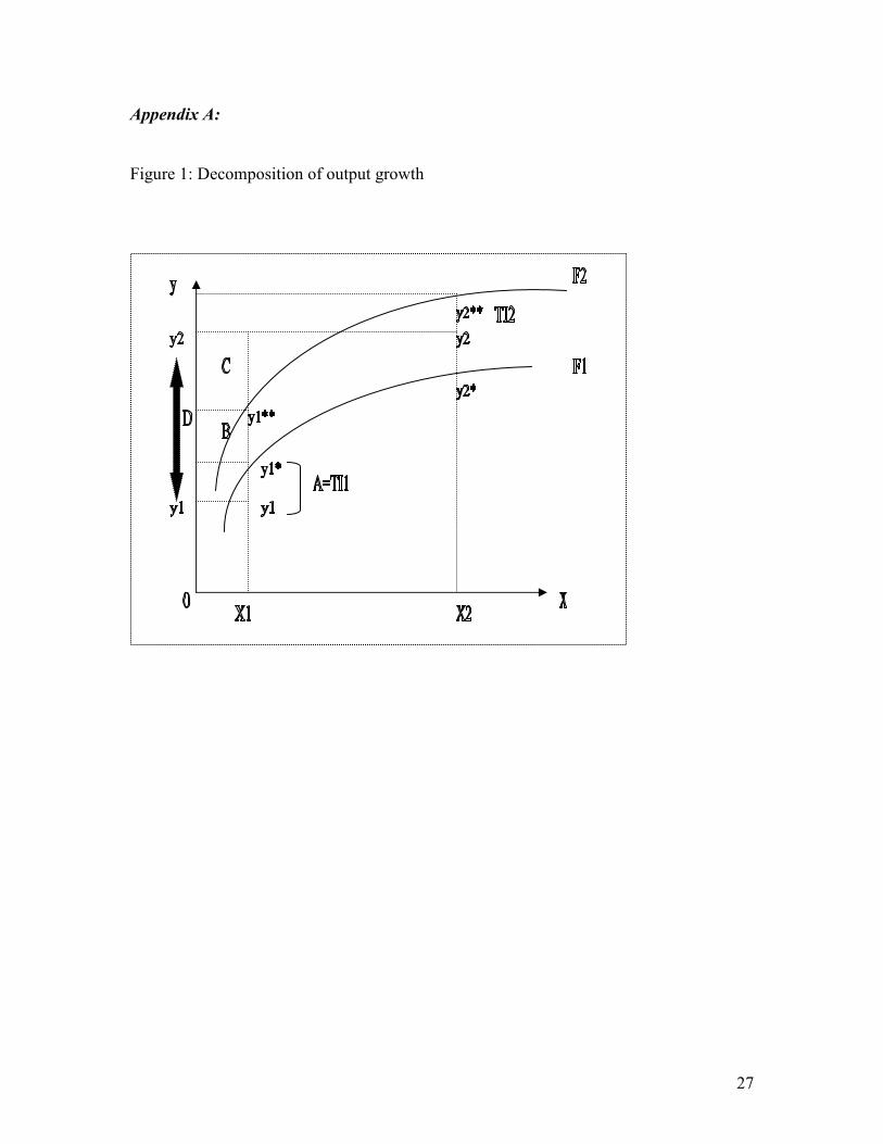
The decomposition of total output growth is graphically illustrated in Figure 1,

following the work by Kalirajan, Obwona, and Zhao (1996) and Wu (2000). In period 1

and 2, the given firm faces production frontiers F1 and F2 respectively. If production is

technically efficient, output would be y1* in period 1 and y2** in period 2. On the other

hand, if production is technically inefficient and does not operate on its frontier, then

realized output is only y1 in period 1 and y2 in period 2. Technical inefficiency (TI) is

measured by the vertical distance between the frontier output and the realized output of

the given firm, that is, TI1 in period 1 and TI2 in period 2, respectively. Hence the

change in technical efficiency overtime is the difference between TI1 and TI2.

Technological progress (TP) is measured by the distance between frontier F2 and frontier

F1, that is, (y2**−y2*) using x 2 input levels or (y1**−y1*) using x 1 input levels. The

contribution of input growth to output growth between period 1 and period 2 is denoted

as ∆ y x , which is the distance between y2** and y1**. The total output growth therefore

9

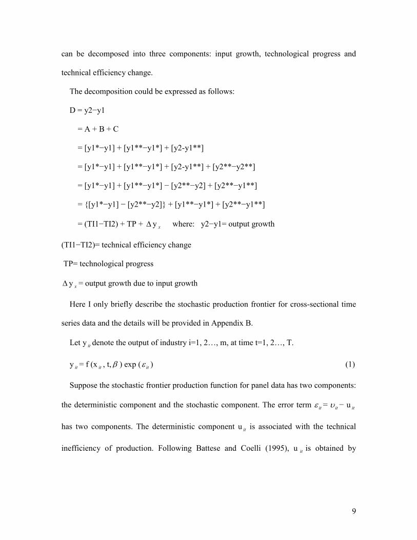
can be decomposed into three components: input growth, technological progress and

technical efficiency change.

The decomposition could be expressed as follows:

D = y2−y1

= A + B + C

= [y1*−y1] + [y1**−y1*] + [y2-y1**]

= [y1*−y1] + [y1**−y1*] + [y2-y1**] + [y2**−y2**]

= [y1*−y1] + [y1**−y1*] − [y2**−y2] + [y2**−y1**]

= {[y1*−y1] − [y2**−y2]} + [y1**−y1*] + [y2**−y1**]

= (TI1−TI2) + TP + ∆ y x where: y2−y1= output growth

(TI1−TI2)= technical efficiency change

TP= technological progress

∆ y x = output growth due to input growth

Here I only briefly describe the stochastic production frontier for cross-sectional time

series data and the details will be provided in Appendix B.

Let y it denote the output of industry i=1, 2…, m, at time t=1, 2…, T.

y it = f (x it , t, β ) exp ( itε ) (1)

Suppose the stochastic frontier production function for panel data has two components:

the deterministic component and the stochastic component. The error term itε = itυ − u it

has two components. The deterministic component u it is associated with the technical

inefficiency of production. Following Battese and Coelli (1995), u it is obtained by

10

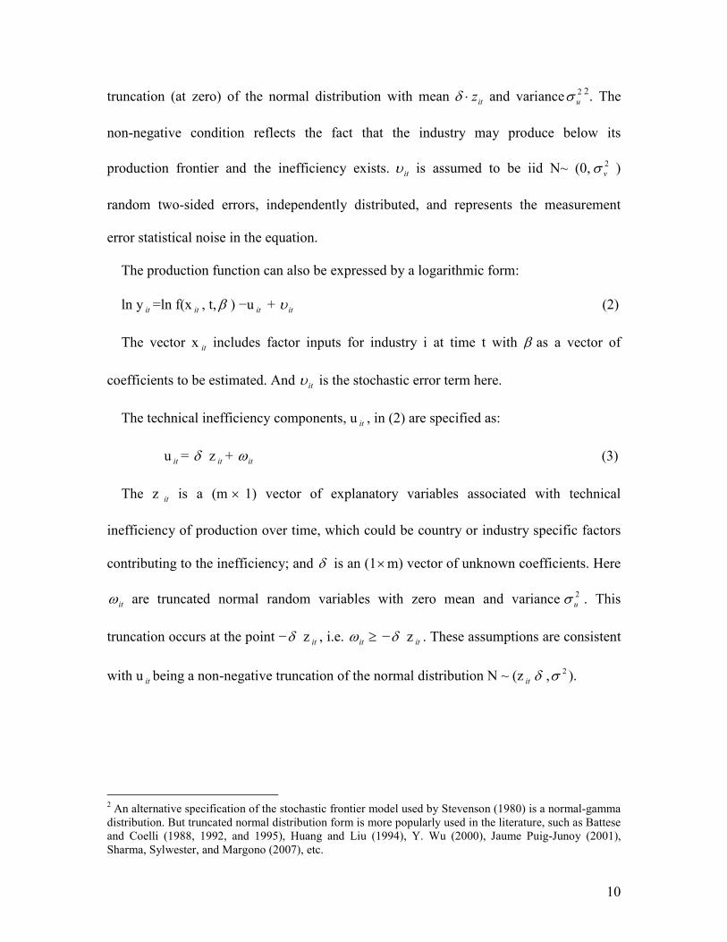
truncation (at zero) of the normal distribution with mean itz⋅δ and variance 2

uσ2. The

non-negative condition reflects the fact that the industry may produce below its

production frontier and the inefficiency exists. itυ is assumed to be iid N~ (0, 2

vσ )

random two-sided errors, independently distributed, and represents the measurement

error statistical noise in the equation.

The production function can also be expressed by a logarithmic form:

ln y it =ln f(x it , t,β ) −u it + itυ (2)

The vector x it includes factor inputs for industry i at time t with β as a vector of

coefficients to be estimated. And itυ is the stochastic error term here.

The technical inefficiency components, u it , in (2) are specified as:

u it = δ z it + itω (3)

The z it is a (m × 1) vector of explanatory variables associated with technical

inefficiency of production over time, which could be country or industry specific factors

contributing to the inefficiency; and δ is an (1×m) vector of unknown coefficients. Here

itω are truncated normal random variables with zero mean and variance 2

uσ . This

truncation occurs at the point −δ z it , i.e. itω ≥ −δ z it . These assumptions are consistent

with u it being a non-negative truncation of the normal distribution N ~ (z it δ , 2σ ).

2 An alternative specification of the stochastic frontier model used by Stevenson (1980) is a normal-gamma

distribution. But truncated normal distribution form is more popularly used in the literature, such as Battese

and Coelli (1988, 1992, and 1995), Huang and Liu (1994), Y. Wu (2000), Jaume Puig-Junoy (2001),

Sharma, Sylwester, and Margono (2007), etc.

11

The method of maximum likelihood3

is used to estimate the parameters of the

stochastic frontier and the technical inefficiency effects simultaneously, which is

originally derived by Battese and Coelli (1992, 1995).

The technical efficiency of production then is defined as follows,

TE it =E [exp (−u it )| itε ] = E [exp (−δ z it −ω it )| itε ] (4)

where itε = itυ − u it , u it ≥ 0

The prediction of the technical efficiencies is based on its conditional expectation,

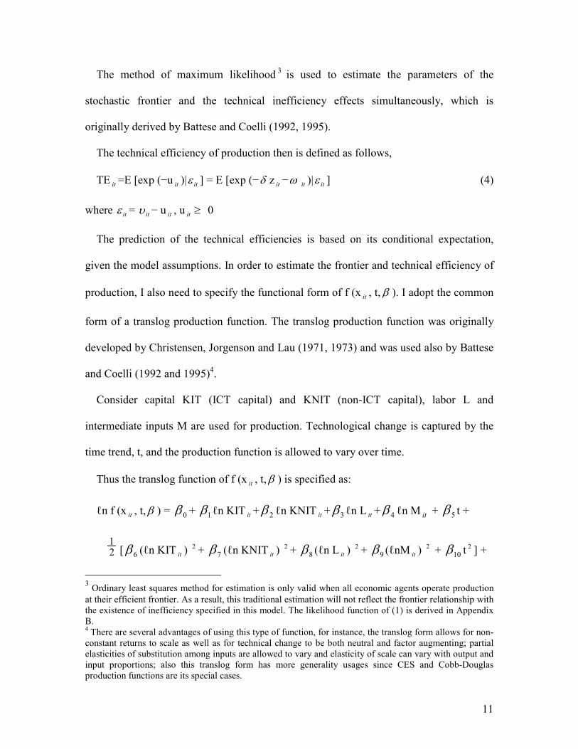
given the model assumptions. In order to estimate the frontier and technical efficiency of

production, I also need to specify the functional form of f (x it , t, β ). I adopt the common

form of a translog production function. The translog production function was originally

developed by Christensen, Jorgenson and Lau (1971, 1973) and was used also by Battese

and Coelli (1992 and 1995)4.

Consider capital KIT (ICT capital) and KNIT (non-ICT capital), labor L and

intermediate inputs M are used for production. Technological change is captured by the

time trend, t, and the production function is allowed to vary over time.

Thus the translog function of f (x it , t,β ) is specified as:

ℓn f (x it , t,β ) = 0β + 1β ℓn KIT it + 2β ℓn KNIT it + 3β ℓn L it + 4β ℓn M it + 5β t +

21

[ 6β (ℓn KIT it ) 2 + 7β (ℓn KNIT it )

2 + 8β (ℓn L it ) 2 + 9β (ℓnM it )

2 + 10β t 2 ] +

3 Ordinary least squares method for estimation is only valid when all economic agents operate production

at their efficient frontier. As a result, this traditional estimation will not reflect the frontier relationship with

the existence of inefficiency specified in this model. The likelihood function of (1) is derived in Appendix

B. 4 There are several advantages of using this type of function, for instance, the translog form allows for non-

constant returns to scale as well as for technical change to be both neutral and factor augmenting; partial

elasticities of substitution among inputs are allowed to vary and elasticity of scale can vary with output and

input proportions; also this translog form has more generality usages since CES and Cobb-Douglas

production functions are its special cases.

12

11β ℓn KIT it * ℓn L it + 12β ℓn KNIT it * ℓn L it + 13β ℓn KIT it * ℓn M it +

14β ℓn KNIT it * ℓn M it + 15β ℓn L it * ℓn M it + 16β t *ℓn KIT it +

17β t *ℓn KNIT it + 18β t *ℓn L it + 19β t*ℓn M it (5)

Then substituting (5) into (2) gives the translog production frontier which will be

estimated by the maximum likelihood method using the computer program, FRONTIER

4.15.

(2) Total factor productivity (TFP)

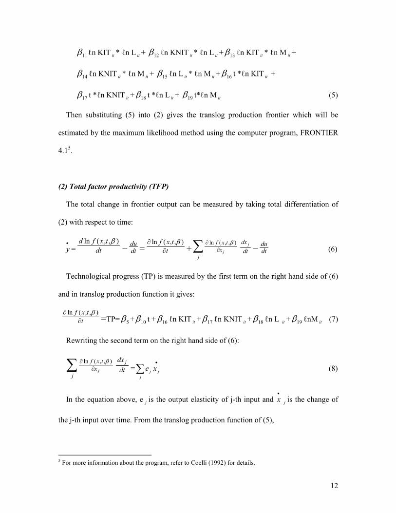
The total change in frontier output can be measured by taking total differentiation of

(2) with respect to time:

•

y = dt

txfd ),,(ln β− dtdu

= t

txf

∂∂ ),,(ln β

+∑ ∂∂

j

x

txf

j

),,(ln β

dt

dx j− dtdu

(6)

Technological progress (TP) is measured by the first term on the right hand side of (6)

and in translog production function it gives:

t

txf

∂∂ ),,(ln β

=TP= 5β + 10β t + 16β ℓn KIT it + 17β ℓn KNIT it + 18β ℓn L it + 19β ℓnM it (7)

Rewriting the second term on the right hand side of (6):

∑ ∂∂

j

x

txf

j

),,(ln β

dt

dx j=∑

•

j

jj xe (8)

In the equation above, e j is the output elasticity of j-th input and •

x j is the change of

the j-th input over time. From the translog production function of (5),

5 For more information about the program, refer to Coelli (1992) for details.

13

eitKIT = )ln(

)ln(

it

it

KIT

Y

∂∂

= 1β + 6β ℓnKIT it + 11β ℓnL it + 13β ℓnM it + 16β t (9)

eitKNIT = )ln(

)ln(

it

it

KNIT

Y

∂∂

= 2β + 7β ℓn KNIT it + 12β ℓnL it + 14β ℓnM it + 17β t (10)

eitL

= )ln(

)ln(

it

it

L

Y

∂∂

= 3β + 8β ℓnL it + 11β ℓn KIT it ++ 12β ℓn KNIT it + 15β ℓnM it + 18β t (11)

e M = )ln(

)ln(

it

it

M

Y

∂∂

= 4β + 9β ℓnM it + 13β ℓnKIT it + 14β ℓn KNIT it + 15β ℓn L it + 19β t (12)

The sum of eitKIT , e KNIT , e

itLand e

itM provides a measure of returns to scale.

The change in technical efficiency is expressed by ∆TE = − dtdu

Thus the total output change equation (6) can be denoted by:

•

y = TP + ∆TE + ∑•

j

jj xe (13)

From the equation above, the overall output change (•

y ) is not only affected by

technological progress and changes in inputs, but also by changes in technical efficiency.

As seen in Figure 1, the TP is positive (negative) if exogenous technical change shifts

the production frontier upward (downward) for a given level of inputs. If dtdu

is negative

(positive), then TE improves (deteriorates) over time.

Denoting •

TFP as output growth unexplained by input growth, the effect of TP and TE

change on TFP change will be:

•

TFP = •

y − ∑•

j

jj xs where s j is input j’s share in production cost. (14)

Substituting (14) into (13), gives:

14

•

TFP = TP + ∆TE + (e-1) j

j

j x•

∑λ +•

−∑ jj

j

j xs )(λ (15)

where e=∑ je denoting a measurement of returns to scale6, ee jj /=λ

When price information is unavailable to determine costs, the allocative efficiency

component, the last term in (15) can not be calculated empirically. Following Sharma et

al. (2007) assumption, assuming ees jj /= for all j, thus reduces (15) to:

•

TFP = TP + ∆TE + ∑•

−j

je

exe j)1( (16)

The sources of total factor productivity growth are decomposed using the above

formula into three components: technological progress, changes in technical efficiency,

and changes in economies of scale.

III: Dataset Description

Using the methodology described in the previous section, I am able to decompose the

TFP growth of total manufacturing industries as well as three sub-group industries using

13 selected OECD industry-level data from 1980 to 2004. The three sub-groups of

manufacturing industries are defined as: Low-tech industries including Food, Beverage

and Tobacco industries and Textile, Textile Products, Leather and Footwear industries;

High-tech industries including Chemical, Rubber, Plastic, Fuel industries, Machinery,

Electrical and Optical Equipments industries, Transport Equipment industries and

Manufacturing NEC; and Resource-based industries including Wood and Wood products

6 Increasing K and L by a% will increase the output by more (less) than a% if there are increasing

(decreasing) returns to scale. If there are constant returns to scale, e=1, and changes in the quantity of

inputs do not affect changes in TFP.

15

industries, Pulp, Paper, Printing and Publishing industries, Other Non-metallic Mineral

industries and Basic Metals, Fabricated metals industries.

The productivity growth is derived based on industrial gross output, so in the

production function the dependent variable is industrial gross output at constant 1995

prices. The independent variables in the production function are labor input measured by

total hours worked by employees; intermediate inputs measured at 1995 prices; ICT

Capital and non-ICT Capital inputs measured by ICT and non-ICT capital services at

1995 prices. All these data are from the EU KLEMS (March 2008) output data file. Gross

output purchasing power parity (PPP) at 1995 prices is used to adjust for the price

differences across countries.

The inefficiency vector z includes an intercept term and some industry-related

variables such as: an R&D intensity term, which is the share of total business expenditure

on R&D (BERD) in value-added; a trade openness term, which is the sum of total exports

and imports share of value-added; a human capital term proxied by the share of hours

worked by high-skilled persons (college or above) engaged; a business cycle factor

proxied by the percentage deviation from the value added trend; and a regulation impact

indicator defined as the growth rate of the regulation impact index. This data is from

OECD statistics regulation impact (RI) indicator datasets, which measures the sectoral

“knock-on” effects of regulation in non-manufacturing sectors7 on all sectors in the

economy. These sectors are the areas in which most economic regulations are

concentrated and where domestic regulations are most relevant to economic activity and

the welfare of consumers. Heavier regulation indicates more negative impacts on

efficiency improvement. In addition, I include some country dummy variables in the

7 Non-manufacturing sectors here include service sectors and energy sectors by OECD definitions.

16

inefficiency function: Euro-European countries (countries which use the Euro as their

currency in the European Union), Non-Euro European countries (countries which do not

use Euro as their currency in the European Union), Oceania countries region (Australia

and Japan) and Canada. The control group is the United States.

The data for value-added, share of hours worked by high skilled persons engaged are

from the EU KLEMS (March 2008) output data file and the data for R&D are from the

OECD STAN BERD tables for each selected country.

IV: Empirical Application

The estimation results of the production frontier function and inefficiency components

are presented in Table 1. The individual coefficients of each variable in the production

function are not readily interpretable given the special form of the translog production

function (Beeson and Husted (1989)). More appropriate interpretation about inputs

elasticities and TFP growth decomposition are presented for this purpose in Table 2 and

Table 6.

[Table 1: Estimates of translog production function and inefficiency components]

A likelihood ratio test is conducted to check whether the Cobb-Douglas production

function is preferred over the translog function. The null hypothesis that the coefficients

6β ─ 19β are equal to zero is rejected at the conventional significance interval with a Chi-

squared statistic of 144.9 is significantly larger than the critical value of 22.36 with 13

degrees of freedom at the 5% significance level.

Also seen from Table 1, γ =68.7% denotes the variance of the inefficiency component

of the error term,2

uσ divided by the total variance22

vu σσ + . It suggests that the majority

17

of the variation in the error term comes from the inefficiency component and is not

measurement error. The likelihood ratio test for the null hypothesis 0=γ is 827.21 with 8

degrees of freedom. This is a mixed Chi-squared statistic with a critical value of 15.51

given 8 degrees of freedom. This result means that the inefficiency term should not be

removed from the production function and thus the model will be inconsistently

estimated only using ordinary least squares.

Most of the coefficients in the inefficiency function are significant at the 95% and 90%

confidence intervals. If the coefficient of a variable is negative, it implies that a specific

variable could help technical efficiency improve over time, and has a positive impact on

TFP growth, vice versa. The coefficients of R&D intensity and trade openness have

negative signs and are both significant, which means they are important determinants of

efficiency improvements over time. They usually have great impacts on competition,

specialization, and technology and knowledge transfer as suggested in many other

productivity research studies. The coefficient of regulation impact growth is significant

and positive, which indicates that more restrictive regulations deteriorate technical

efficiency improvement over time and contribute negatively to the TFP growth given the

sample period. Although the human capital term proxied by the share of high-skilled

persons engaged is not statistically significant in the regression analysis, the coefficient

of this term has the expected negative sign, which means with more educated workers in

the labor force, the industry can achieve better production efficiency of applied

technology. The business cycle factor is negative and statistically significant, which

suggests that technical efficiency improvement is more closely related with economic

fluctuations. Coefficients for most of the country dummy variables are negatively

18

significant, which indicates the experience of technical efficiency improvements in those

countries.

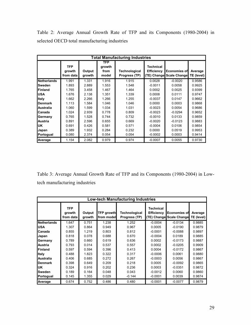
Detailed decompositions of TFP growth in 13 OECD countries total manufacturing

industries from 1980 to 2004 are reported in Table 2. The first column represents the

annual average TFP growth rate calculated empirically. The industrial gross output

growth is in column 2. The model estimated annual average TFP growth is listed in

column 3. The contributions of technological progress, technical efficiency change and

economies of scale to TFP growth are presented in column 4, 5 and 6 respectively,

followed by the level of average technical efficiency. The model residual can therefore be

calculated by the difference of column 1 and 3.

[Table 2: Average Annual Growth Rate of TFP and its Components (1980-2004) in

selected OECD total manufacturing industries]

All countries’ total manufacturing industries experienced positive TFP growth in the

sample period, in which technological progress contributed most. Therefore technological

progress played a dominant role in contributing to TFP growth. In another words, most of

the TFP growth was due to outward shifts of the production function rather than moves

towards it. The average technical efficiency level is close to one in all sample countries,

indicating that the potential TFP growth will mainly be achieved by technological

progress (innovation). Both the changes in efficiency and economies of scale have

minuscule contributions to TFP growth from the estimation.

The innovation efforts of manufacturing industries differ a lot across the selected

OECD countries. During the study period, Netherlands had the highest technological

growth at a 1.9% annualised rate while Portugal ranked the last at 0.05% annual growth

19

in technological progress. The average technological progress is 0.974% per year in the

sample countries manufacturing. Generally speaking, a country experiencing very low

TFP growth such as Portugal should focus on technology innovation along with

improving efficiency to produce. If high rates of technological progress coexisted with

deteriorating technical efficiency in countries like Canada and Italy, then increasing the

efficiency given existing technology is required. For other countries with somewhat

efficiency improvement but relatively low technological progress such as Japan, more

efforts could be put into technology innovations to increase TFP growth over time.

The two countries in North America, Canada and the U.S. did not perform very

competitively in terms of TFP growth across the sample OECD countries. Canadian and

U.S. total manufacturing ranked 8th

and 4th

, respectively, among 13 OECD countries in

average TFP growth. The average TFP growth and its components in Canada were lower

than the 13 OECD country average. Moreover, the TFP growth rate of Canadian total

manufacturing industries was only 57 percent of their U.S. counterparts. Total

manufacturing industries in Canada experienced much slower technology progress than

in the U.S. (60 percent of the U.S.). Negative changes in technical efficiency and

economies of scale also worsened TFP growth in Canada. Canadian manufacturing

experienced lower than OECD average technical efficiency change. As it is well known

that both R&D expenditure is assumed to be a major driver of the fundamental innovation

and efficiency improvement, and ICT capital contributes significantly both directly and

indirectly to TFP growth8, the differences of R&D expenditure and ICT capital share of

total non-residential investment could partly explain the TFP gap between Canadian and

8 ICT capital contributes directly through capital accumulation and capital deepening. They also impact on

innovation indirectly through spillovers effects.

20

the U.S. manufacturing industries. The average ICT share was significantly bigger in the

U.S. than in Canadian manufacturing industries. Canadian manufacturing industries had

less than 10 percent of their U.S. counterparts invested on ICT assets during the sample

period. The R&D share of value-added in Canadian manufacturing industries was only

one third of their U.S. counterparts in 2004. The R&D share averaged 4 percent in

Canada while it averaged 10 percent in the U.S. manufacturing industries. The estimation

results also suggest that the share of high-skilled labor positively contributes to efficiency

improvement. In Canada, the total working hour share of high-skilled persons was only

half of that in the U.S. The difference in labor skills could therefore determine the

difference in TFP growth between these two countries.

To have a closer look at TFP performances in different groups of manufacturing

industries, I also decompose TFP growths in three sub-group manufacturing industries

(low-tech, high-tech and resource-based manufacturing industries) as defined previously.

Overall, the sub-group manufacturing showed similar patterns in terms of the sources of

TFP growth as the total manufacturing. Table 3, Table 4 and Table 5 provide the detailed

summaries for these results.

[Table 3: Average Annual Growth Rate of TFP and its Components (1980-2004) in

Low-tech manufacturing industries]

Across the OECD low-tech manufacturing industries, nearly all TFP growth comes

from technological progress, and both technical efficiency change and economies of scale

contribute negatively to TFP growth. The magnitude of TFP growth in the low-tech

group is much smaller than total manufacturing industries. The U.S. and Canadian low-

tech industries performed relatively competitively in the selected OECD countries,

21

although the TFP growth in Canada was still slightly lower than in the U.S. The total

hours worked by high-skilled persons engaged in Canada were only 60 percent of that in

the U.S. The gap in the R&D expenditure was large and up to 40 percent. These facts

may partly explain the difference in the contribution of technical efficiency to TFP

growth between these two countries.

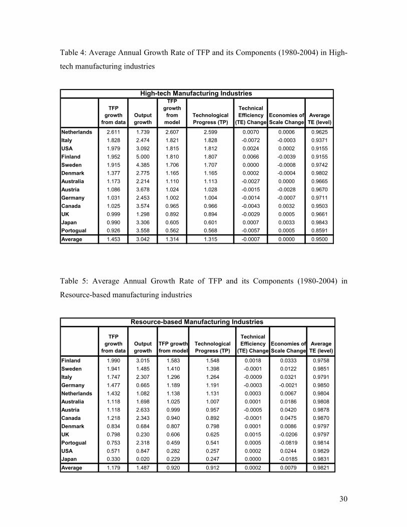
[Table 4: Average Annual Growth Rate of TFP and its Components (1980-2004) in

High-tech manufacturing industries]

In Table 4, high-tech manufacturing registered the highest average TFP growth in the

sub-group analysis, which posted nearly three times the TFP growth of the low-tech

sector and one and a half times of the resource-based sector. The majority of the TFP

growth was from technology innovation. The high-tech sector played an important role in

the total manufacturing industries across these OECD countries. Average TFP growth in

the Netherlands was nearly five times of that in Portugal. There were five countries

(Netherlands, Italy, U.S., Finland and Sweden) high-tech sector had the above average

technological progress during the sample period. Though this group of manufacturing

experienced rapid technological progress, it was characterized by lower efficiency. This

low level of efficiency was consistent with the estimated contribution of negative

efficiency change to TFP growth. Since many countries experienced negative technical

efficiency change, improving technical efficiency of production given the current

technology could help these countries grow at a higher rate. Canadian high-tech

industries only ranked 10th

out of 13 countries and lagged in TFP growth behind many

other countries. Slower technological progress significantly determined lower TFP

growth in the Canadian high-tech industries. Compared with their U.S. counterparts, TFP

22

growth in Canada was merely 53 percent of that in the U.S. The ICT intensity gap

between Canadian and U.S. high-tech sector was significantly large. The ICT share of

total non-residential investment averaged 8 percent in the U.S., while it was less than one

percent in Canadian high-tech industries. The share of high-skilled persons working

hours in Canada was only 59 percent of that in the U.S. All of these factors may

adversely affect the TFP growth in Canadian high-tech sector.

[Table 5: Average Annual Growth Rate of TFP and its Components (1980-2004) in

Resource-based manufacturing industries]

Table 5 shows the decompositions of TFP growth in resource-based manufacturing

industries. Finland ranked 1st and Japan ranked last in TFP growth. Technological

progress still significantly contributed to TFP growth in this sub-sector. Although

Canadian resource-based manufacturing performed much better than their U.S.

counterparts, it still ranked 8th

out of 13 countries, with lower than average technology

innovation. The change in economies of scale was highest in Canada among all other

OECD countries, while the technical efficiency component negatively contributed to TFP

growth. Canada is known as a natural resource exporting country with comparative

advantage in its natural resource production. Innovation is the most critical driver for

enhanced productivity and competitiveness. To stay in a competitive position, the

Canadian resource-based sector should invest more in ICT capital and human capital,

conduct more R&D and adopt new production process that improve technical efficiency

according to the estimation results.

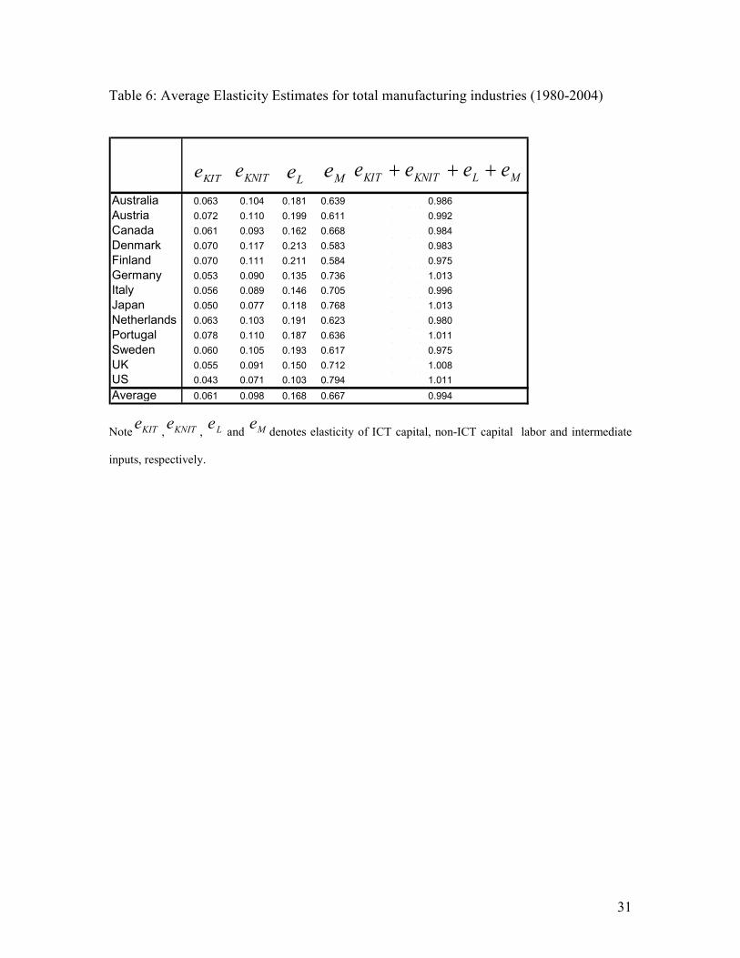
[Table 6: Average Elasticity Estimates for total manufacturing industries (1980-2004)]

23

Finally, in Table 6, the average contribution from economies of scale to TFP growth is

provided for total manufacturing industries in each country during the period studied. The

elasticities of both types of capital, labor and intermediate inputs for each country are

reported at the average level during the sample periods of 1980-2004. The average ICT

capital share of production was 0.061, the non-ICT capital share was 0.098, the labor

share was 0.168 and the intermediate inputs share was 0.667, which implies constant

returns to scale for production function. This also explains why the component of

economies of scale was minuscule in TFP growth since this component dropped out of

equation (15) when 1=e . Intermediate inputs contributed the most in the production

function since our productivity analysis was based on the gross output method.

V: Conclusion

This paper decomposes total factor productivity growth into technological progress,

efficiency improvement and economies of scale for 13 selected OECD manufacturing

industries, including Canada. This study not only estimates the average TFP growth

across countries, but also investigates the driving forces for productivity growth.

The regression results suggest that the R&D share of value-added, trade openness,

business cycles and smart regulation all have contributed to TFP growth through the

efficiency improvement channel. Overall, TFP growth in 13 selected OECD countries is

mainly due to outward shifts of the production function than to movement towards it.

Intuitively, improvement in efficiency is limited since TFP growth can only be driven to

the production possibility curve; once the production is carried out at the most efficient

level given the existing level of technology, no further improvement in TFP can be

24

achieved. On the other hand, changes in technological progress can be realized over time

and continue infinitely. Thus, once the frontier is reached given the current technology,

long-run growth will come only from technological progress. Changes in economies of

scale and efficiency improvement are minor contributors to TFP growth. The average

total share of capital, labor and intermediate inputs indicates constant returns to scale in

the selected countries’ manufacturing industries. These features of TFP growth and its

sources have shown similar patterns in the three sub-group manufacturing industries

studies.

Canadian manufacturing industries ranked 8 out of 13 OECD countries in terms of

average TFP growth. Moreover, TFP growth in Canada lagged behind the U.S. in most

manufacturing industries, especially in the high-tech manufacturing industries. Canadian

manufacturing industries only had some advantage in the resource-based sectors.

Canadian manufacturing industries experienced just half of the technological progress

compared to the U.S. during the period studied, and they were operating less efficiently

than their U.S. counterparts. The ICT capital intensity, R&D share of value-added gaps

and skills difference between the U.S. and Canadian manufacturing industries were large

and could result in TFP growth gap through innovation and efficiency improvements.

These U.S.-Canada comparative findings are consistent with the recent study by Rao,

Tang, Wang and Hao (2008) of Industry Canada. Their estimates suggest that Canada is

more productive than the U.S. in a number of resource-based industries, but trails the

United States in high-tech manufacturing industries.

The results of this study also point to the importance of efficiency improvements to the

TFP growth given available technologies. In this sense, our study contributes not only to

25

identify the sources of TFP growth which are critical to finding future growth potentials,

but also to practically interpret the effects of policies to promote productivity and

innovation.

References:

Aigner, D.J., Lovell, C.A.K., and Schmidt, P.J. (1977) “Formulation and Estimation of Stochastic Frontier

Models”, Journal of Econometrics, 6(1), 21-37

Battese, G. E. and Coelli, T. J. (1992) “Frontier Production Functions, Technical Efficiency and Panel

Data: with Application to Paddy Farmers in India”, Journal of Productivity Analysis, 3, 153-169

Battese, G. E. and Coelli, T. J. (1995) “A Model for Technical Inefficiency Effects in a Stochastic Frontier

Production Function for Panel Data”, Empirical Economics, 20, 325-332

Bauer, Paul, W. (1990) “Decomposing TFP Growth in the Presence of Cost Inefficiency, Nonconstant

Retums to Scale, and Technological Progress”, the Journal of Productivity Analysis, 1, 287-299

Beeson, P. E., and Husted, S. (1989) “Patterns and Determinants of Productivity Efficiency in State

Manufacturing”, Journal of Regional Science, 29, 15-28

Brock, G. (2001) “an Econometric Look at Inefficiency among U.S. States”, Review of Regional Studies,

31, 95-107

Domazlicky, B.R. and Weber, W.L. (1997) “Total Factor Productivity in the Contiguous United States,

1977-1986”, Journal of Regional Science, 37, 213-233

Fare, Rolf; Grosskopf, Shawna; Norris, Mary and Zhang, Zhongyang (1994) “Productivity Growth,

Technical Progress, and Efficiency Change in Industrialized Countries”, the American Economic Review,

Vol.84, No.1, 66-83

Ferrell, M.J. (1957), “the Measurement of Productive Efficiency”, Journal of the Royal Statistical Society,

Series A, General, 120, 253-282

Greene, W.H. (1980a), “Maximum Likelihood Estimation of Econometric Frontier Functions”, Journal of

Econometrics, vol.19, no.1, 37-57

Greene, W.H. (1980b), “On the Estimation of a Flexible Frontier Production Model”, Journal of

Econometrics, vol.19, no.1, 101-117

Huang CJ, Liu J-T (1994) “Estimation of a Non-neutral Stochastic Frontier Production Function”, Journal

of Productivity Analysis, 5: 171-180

26

Hutlen, C.R. and Robert M.S. (1984) “Regional Productivity Growth in U.S. Manufacturing, 1951-78”, the

American Economic Review, 74, 152-162

Jefferson, G.H., Rawski, T.G., & Zheng, Y (1996) “Chinese Industrial Productivity: Trends, Measurement

issues and recent developments”, Journal of Comparative Economics, 23, 146-180

Koop, G., Osiewalski, J., and Steel, M.F.J. (1999) “the Components of Output Growth: A Stochastic

Frontier Analysis”, Oxford Bulletin of Economics and Statistics, 61, 455-487

Koop, G., Osiewalski, J., and Steel, M.F.J. (2000) “Modelling the Sources of Output Growth in a Panel of

Countries”, Journal of Business and Economic Statistics, 18, 284-299

Kumbhakar SC, Ghosh S, McGuckin JT (1991) “A Generalized Production Frontier Approach for

Estimating Determinants of Inefficiency in US Dairy Farms”, Journal of Business and Economic Statistics,

9: 279-286

Lau, K.T. and Brada, J.C. (1990) “Technological Progress and Technical Efficiency in Chinese Industry

Growth: a Frontier Production Function Approach”, China Economic Review, 1, 113-124

Lau, L. and Kim, J.I. (1994) “the Sources of Economic Growth in the East Asian Newly Industrialized

Countries”, Journal of the Japanese and International Economies, 8, 235-271

Meeusen, W., and van den Broeck, J. (1977) “Efficiency Estimation from Cobb-Douglas Production

Function with Compose Error”, International Economic Review, 18(2), 435-444

Nishimizu, M., & Page, J.M. (1982) “Total Factor Productivity Growth, Technological Progress and

Technical Efficiency Change: Dimensions of Productivity Change in Yugoslavia, 1965-78”, Economic

Journal, 92, 920-936

Osiewalski, J., Koop, G., and Steel, M.F.J. (1998) “A Stochastic Frontier Analysis of Output Level and

Growth in Poland and Western Economies”, Working paper, Department of Economics, Tilburg University

Pitt MM, Lee M-F (1981) “The Measurement and Sources of Technical Inefficiency in the Indonesian

Weaving Industry”, Journal of Development Economics, 9: 43-64

Puig-Junoy, J. (2001) “Technical Inefficiency and Public Capital in U.S. States: A Stochastic Frontier

Approach”, Journal of Regional Science, 41, 75-96

Reifschneider D, Stevenson R (1991) “Systematic Departures from the Frontier: A Framework for the

Analysis of Firm Inefficiency”, International Economic Review, 32: 715-723

Sharma, Subhash C., Sylwester Kevin, Margono Heru (2007) “Decomposition of Total Factor Productivity

Growth in U.S. states”, The Quarterly Review of Economics and Finance, 47, 215-241

Wu, Yanrui (2000) “is China’s Economic Growth Sustainable? A Productivity Analysis”, China Economic

Review, 11, 278-296

27

Appendix A:

Figure 1: Decomposition of output growth

28

Table 1: Estimates of translog production function and inefficiency components

Parameter Variable Estimate Standard Error

Production Function

Beta 0 Intercept 1.103 0.759

Beta 1 ln(KIT) 0.063 0.069

Beta2 ln(KNIT) 0.128 0.171

Beta 3 ln(L) -0.383 0.263

Beta 4 ln(M) 1.191* 0.343

Beta 5 t -0.013* 0.007

Beta 6 ln(KIT)^2/2 -0.006* 0.003

Beta 7 ln(KNIT)^2/2 0.132* 0.022

Beta 8 ln(L)^2/2 0.028 0.030

Beta 9 ln(M)^2/2 -0.032 0.044

Beta 10 t^2/2 0.0005* 0.000

Beta 11 ln(KIT)ln(L) 0.083* 0.015

Beta 12 ln(KNIT)ln(L) -0.035 0.040

Beta 13 ln(KIT)ln(M) -0.013 0.018

Beta 14 ln(KNIT)ln(M) -0.171* 0.057

Beta 15 ln(L)ln(M) 0.237* 0.061

Beta 16 tln(KIT) 0.003* 0.001

Beta 17 tln(KNIT) 0.006* 0.001

Beta 18 tln(L) -0.024* 0.002

Beta 19 tln(M) 0.020* 0.002

Inefficiency Components

Delta 0 Intercept -0.027 0.033

Delta 1 Business cycles -0.163* 0.061

Delta 2 High skilled hours share -0.001 0.014

Delta 3 R&D/VA -1.538* 0.185

Delta 4 Trade openness -0.013* 0.004

Delta 5 Regulation Indicator 0.041* 0.014

Delta 6 Euro-European 0.045* 0.017

Delta 7 Non-Euro European -0.020* 0.017

Delta 8 Oceania -0.065* 0.020

Delta 9 Canada -0.042* 0.019

Sigma square Variance of Inefficiency 0.001* 0.000

Gamma 0.687* 0.079

* denotes significant at both 5% and 10% levels

22

2

vu

u

σσ

σ

+

29

Table 2: Average Annual Growth Rate of TFP and its Components (1980-2004) in

selected OECD total manufacturing industries

TFP

growth

from data

Output

growth

TFP

growth

from

model

Technological

Progress (TP)

Technical

Efficiency

(TE) Change

Economies of

Scale Change

Average

TE (level)

Netherlands 1.991 1.331 1.916 1.915 0.0028 -0.0020 0.9586

Sweden 1.893 2.889 1.553 1.548 -0.0011 0.0058 0.9925

Finland 1.765 3.458 1.467 1.464 0.0002 0.0025 0.9399

USA 1.676 2.138 1.351 1.339 0.0008 0.0111 0.9747

Italy 1.662 2.266 1.266 1.255 -0.0037 0.0147 0.9662

Denmark 1.113 1.584 1.046 1.046 0.0000 0.0003 0.9868

Australia 1.060 1.599 1.034 1.031 -0.0023 0.0054 0.9686

Canada 1.024 2.939 0.778 0.809 -0.0023 -0.0294 0.9652

Germany 0.765 1.528 0.744 0.732 -0.0010 0.0133 0.9859

Austria 0.891 2.596 0.655 0.669 -0.0020 -0.0123 0.9883

UK 0.691 0.426 0.581 0.571 -0.0004 0.0106 0.9854

Japan 0.389 1.932 0.284 0.232 0.0000 0.0519 0.9953

Portogual 0.080 2.374 0.054 0.054 -0.0002 0.0003 0.9414

Average 1.154 2.082 0.979 0.974 -0.0007 0.0055 0.9730

Total Manufacturing Industries

Table 3: Average Annual Growth Rate of TFP and its Components (1980-2004) in Low-

tech manufacturing industries

TFP

growth

from data

Output

growth

TFP growth

from model

Technological

Progress (TP)

Technical

Efficiency

(TE) Change

Economies of

Scale Change

Average

TE (level)

Netherlands 1.647 0.751 1.238 1.252 -0.0004 -0.0134 0.9885

USA 1.307 0.864 0.949 0.967 0.0005 -0.0190 0.9879

Canada 0.855 1.219 0.803 0.812 -0.0001 -0.0088 0.9897

Japan 0.818 0.078 0.688 0.670 -0.0004 0.0189 0.9885

Germany 0.789 0.660 0.619 0.636 0.0002 -0.0173 0.9887

Austria 0.793 0.014 0.537 0.557 0.0002 -0.0205 0.9909

Finland 0.597 0.594 0.396 0.413 0.0004 -0.0172 0.9867

Italy 0.488 1.823 0.322 0.317 -0.0006 0.0061 0.9880

Australia 0.406 0.685 0.272 0.267 -0.0003 0.0056 0.9867

Denmark 0.398 0.649 0.209 0.218 0.0005 -0.0092 0.9865

UK 0.324 0.916 0.202 0.236 0.0003 -0.0351 0.9872

Sweden 0.189 0.164 0.048 0.043 -0.0012 0.0060 0.9860

Portogual 0.145 1.355 0.029 -0.144 -0.0001 0.0039 0.9874

Average 0.674 0.752 0.486 0.480 -0.0001 -0.0077 0.9879

Low-tech Manufacturing Industries

30

Table 4: Average Annual Growth Rate of TFP and its Components (1980-2004) in High-

tech manufacturing industries

TFP

growth

from data

Output

growth

TFP

growth

from

model

Technological

Progress (TP)

Technical

Efficiency

(TE) Change

Economies of

Scale Change

Average

TE (level)

Netherlands 2.611 1.739 2.607 2.599 0.0070 0.0006 0.9625

Italy 1.828 2.474 1.821 1.828 -0.0072 -0.0003 0.9371

USA 1.979 3.092 1.815 1.812 0.0024 0.0002 0.9155

Finland 1.952 5.000 1.810 1.807 0.0066 -0.0039 0.9155

Sweden 1.915 4.385 1.706 1.707 0.0000 -0.0008 0.9742

Denmark 1.377 2.775 1.165 1.165 0.0002 -0.0004 0.9802

Australia 1.173 2.214 1.110 1.113 -0.0027 0.0000 0.9665

Austria 1.086 3.678 1.024 1.028 -0.0015 -0.0028 0.9670

Germany 1.031 2.453 1.002 1.004 -0.0014 -0.0007 0.9711

Canada 1.025 3.574 0.965 0.966 -0.0043 0.0032 0.9503

UK 0.999 1.298 0.892 0.894 -0.0029 0.0005 0.9661

Japan 0.990 3.306 0.605 0.601 0.0007 0.0033 0.9843

Portogual 0.926 3.558 0.562 0.568 -0.0057 0.0005 0.8591

Average 1.453 3.042 1.314 1.315 -0.0007 0.0000 0.9500

High-tech Manufacturing Industries

Table 5: Average Annual Growth Rate of TFP and its Components (1980-2004) in

Resource-based manufacturing industries

TFP

growth

from data

Output

growth

TFP growth

from model

Technological

Progress (TP)

Technical

Efficiency

(TE) Change

Economies of

Scale Change

Average

TE (level)

Finland 1.990 3.015 1.583 1.548 0.0018 0.0333 0.9758

Sweden 1.941 1.485 1.410 1.398 -0.0001 0.0122 0.9851

Italy 1.747 2.307 1.296 1.264 -0.0009 0.0321 0.9791

Germany 1.477 0.665 1.189 1.191 -0.0003 -0.0021 0.9850

Netherlands 1.432 1.082 1.138 1.131 0.0003 0.0067 0.9804

Australia 1.118 1.698 1.025 1.007 0.0001 0.0186 0.9808

Austria 1.118 2.633 0.999 0.957 -0.0005 0.0420 0.9878

Canada 1.218 2.343 0.940 0.892 -0.0001 0.0475 0.9870

Denmark 0.834 0.684 0.807 0.798 0.0001 0.0086 0.9797

UK 0.798 0.230 0.606 0.625 0.0015 -0.0206 0.9797

Portogual 0.753 2.318 0.459 0.541 0.0005 -0.0819 0.9814

USA 0.571 0.847 0.282 0.257 0.0002 0.0244 0.9829

Japan 0.330 0.020 0.229 0.247 0.0000 -0.0185 0.9831

Average 1.179 1.487 0.920 0.912 0.0002 0.0079 0.9821

Resource-based Manufacturing Industries

31

Table 6: Average Elasticity Estimates for total manufacturing industries (1980-2004)

Australia 0.063 0.104 0.181 0.639 0.986

Austria 0.072 0.110 0.199 0.611 0.992

Canada 0.061 0.093 0.162 0.668 0.984

Denmark 0.070 0.117 0.213 0.583 0.983

Finland 0.070 0.111 0.211 0.584 0.975

Germany 0.053 0.090 0.135 0.736 1.013

Italy 0.056 0.089 0.146 0.705 0.996

Japan 0.050 0.077 0.118 0.768 1.013

Netherlands 0.063 0.103 0.191 0.623 0.980

Portugal 0.078 0.110 0.187 0.636 1.011

Sweden 0.060 0.105 0.193 0.617 0.975

UK 0.055 0.091 0.150 0.712 1.008

US 0.043 0.071 0.103 0.794 1.011

Average 0.061 0.098 0.168 0.667 0.994

mlk eee ++

mlk eee ++

mlk eee ++

mlk eee ++

mlk eee ++

mlk eee ++

mlk eee ++

mlk eee ++

mlk eee ++

mlk eee ++

mlk eee ++

mlk eee ++

MeKITe KNITeLe MLKNITKIT eeee +++

Note KITe, KNITe

, Le and Me denotes elasticity of ICT capital, non-ICT capital labor and intermediate

inputs, respectively.

32

Appendix B:

The results of this part were originally derived by Battese and Coelli (1993, 1995) and

rephrased by S.C. Sharma et al. (2007).

Consider the stochastic frontier function:

ℓn Y it = ℓnf(x it , t, β ) + itυ −u it where region i=1, 2,…, m and time t=1, 2,…, T. (a.1)

Let y it = ℓn Y it for simplicity.

Given the assumption of u it (normal distribution truncated at zero) and itυ (normal

distribution), the density function for u it and itυ are:

g 1 (υ ) = πσυ 2

1exp (− 2

2

2 υσυ

), −∞ <υ < ∞ (a.2)

g 2 (u) = )/(2

1

uz σδπσυ Ψ exp (− )2

2

2

)(

u

zu

σ

δ−,u≥0 (a.3)

where Ψ (·) represents the standard normal distribution function for the random

variable and the subscripts, t and i are omitted to ease notation. The joint density of u and

ε is:

h (ε , u) = )/(2

))]}/()(())/())[((2/1(exp{ 2222

uu

u

z

zuu

σδσπσσδσε

υ

υ

Ψ−++−

, u≥0 (a.4)

Simplifying (a.4) gives:

h(ε , u) = )/(2

))]}/()(())/())[((2/1(exp{ 2222*

2*

uu

u

z

zu

σδσπσσσδεσµ

υ

υΨ

+++−− ,u≥0 (a.5)

where *µ = 22

22

υ

υ

σσ

σδεσ

+

+−

u

u z and 2

*σ = 22

22

υ

υ

σσ

σσ

+u

u

(a.6)

From (a.5), the density function of −=υε u is:

h 1 (ε )= ∫∞

0),( duuh ε = )/(2

)]})/()/()/)[((2/1(exp{ 2**

222

uu

u

z

z

σδσσπ

σµσδσε

υ

υ

Ψ

−+−×

π

σµ

2

)))/))((2/1(exp(0

2*

2*∫

∞−− duu

(a.7)

After simplifying, (a.7) becomes:

h 1 (ε )=)}/(/)/({2

)))}(2/))((2/1(exp{

**22

222

σµσδσσπ

σσδε

υ

υ

ΨΨ+

++−

uu

u

z

z (a.8)

Using the (a.5) and (a.8), the conditional density function of u given ε is:

33

f(u|ε )= )/(2

)}/))((2/1(exp{

***

2*

2*

σµσπ

σµ

Ψ

−− u , u≥0 (a.9)

From (a.9), the conditional expectation of exp (−u it ) given itε will be:

TE it = E (e itu− | itε ) = )/(

])/()[(

**,

***,

σµσσµ

it

it

Ψ

−Ψexp ( it*,µ− +

21

*σ ) (a.10)

where we reintroduce the subscripts for clarify the expression for the i-th region at the t-

th period, so (a.6) becomes:

it*,µ = *µ = 22

22

υ

υ

σσ

σδεσ

+

+−

u

ititu z

and 2

*σ = 22

22

υ

υ

σσ

σσ

+u

u

(a.11)

Now the density function for output value y it in (a.1) can be obtained from (a.8):

f(y it ) = )](/)()[(2

)}/(]),,(ln)[2/1(exp{

*,22

222

ititu

uititit ztxfy

ξξσσπ

σσδβ

υ

υ

ΨΨ+

++−− (a.12)

where itξ = u

itz

σδ

, it*,ξ = *

*,

σµ it

, and it*,µ = 22

22)],,(ln[

υ

υ

σσ

βσδσ

+

−−

u

itituit txfyz (a.13)

Let y i = (y 1i , y 2i , ..., y it )’ be a T×1 vector of the log of output of the i-th region and let

y = (y1 ’, y 2 ’, ... , y m ’)’ be the (mT×1) vector of the log of output of all regions over T

time periods. Then the logarithm of the likelihood function of the sample observations y

is given by:

ℓnL (θ, y) = −21 m T [ℓn2π + ℓn ( 22

uv σσ + )]

−21 { ))]}(ln)((ln[ *,

1 1

)),,(ln(22

2

itit

m

i

T

t

ztxfy

u

ititit ξξυσσ

δβ Ψ−Ψ+∑∑= =

+

+− (a.14)

where θ = (β s ’, sδ ’, 2

uσ , 2

υσ )

The log likelihood function in (a.14) will be estimated by Frontier 4.1 software. Using the

estimated parameter values, TE in (a.10) then will be estimated, as well as the

components of TFP growth in equations (9), (10), (11), (12) and (16).