Contributed Paper

Specimen-Based Modeling, Stopping Rules, andthe Extinction of the Ivory-Billed WoodpeckerNICHOLAS J. GOTELLI,∗ ANNE CHAO,† ROBERT K. COLWELL,‡ WEN-HAN HWANG,§AND GARY R. GRAVES#∗Department of Biology, University of Vermont, Burlington, VT 05405, U.S.A., email ngotelli@uvm.edu†Institute of Statistics, National Tsing Hua University, Hsin-Chu 30043, Taiwan‡Department of Ecology and Evolutionary Biology, University of Connecticut, Storrs, CT 06269-3043, U.S.A.§Department of Applied Mathematics, National Chung Hsing University, Tai-Chung 402, Taiwan#Department of Vertebrate Zoology, MRC-116, National Museum of Natural History, Smithsonian Institution, PO Box 37012,Washington, D.C. 20013-7012, U.S.A., and Center for Macroecology, Evolution, and Climate, University of Copenhagen, Denmark

Abstract: Assessing species survival status is an essential component of conservation programs. We deviseda new statistical method for estimating the probability of species persistence from the temporal sequence ofcollection dates of museum specimens. To complement this approach, we developed quantitative stopping rulesfor terminating the search for missing or allegedly extinct species. These stopping rules are based on surveydata for counts of co-occurring species that are encountered in the search for a target species. We illustrateboth these methods with a case study of the Ivory-billed Woodpecker (Campephilus principalis), long assumedto have become extinct in the United States in the 1950s, but reportedly rediscovered in 2004. We analyzedthe temporal pattern of the collection dates of 239 geo-referenced museum specimens collected throughoutthe southeastern United States from 1853 to 1932 and estimated the probability of persistence in 2011 as<6.4 × 10−5, with a probable extinction date no later than 1980. From an analysis of avian census data(counts of individuals) at 4 sites where searches for the woodpecker were conducted since 2004, we estimatedthat at most 1–3 undetected species may remain in 3 sites (one each in Louisiana, Mississippi, Florida). Ata fourth site on the Congaree River (South Carolina), no singletons (species represented by one observation)remained after 15,500 counts of individual birds, indicating that the number of species already recorded (56)is unlikely to increase with additional survey effort. Collectively, these results suggest there is virtually nochance the Ivory-billed Woodpecker is currently extant within its historical range in the southeastern UnitedStates. The results also suggest conservation resources devoted to its rediscovery and recovery could be betterallocated to other species. The methods we describe for estimating species extinction dates and the probabilityof persistence are generally applicable to other species for which sufficient museum collections and field censusresults are available.

Keywords: avian censuses, Campephilus principalis, extinction estimation, extinction probability, Ivory-billedWoodpecker, museum specimens, species richness estimators, stopping rules

Modelado Basado en Especımenes, Reglas de Decision y la Extincion de Campephilus principalis

Resumen: La evaluacion del estatus de supervivencia de las especies es un componente esencial de losprogramas de conservacion. Disenamos un nuevo metodo estadıstico para estimar la probabilidad de lapersistencia de especies a partir de la secuencia temporal de datos de colecta de especımenes de museo.Para complementar este metodo, desarrollamos reglas de decision cuantitativas para terminar la busquedade especies ausentes o presuntamente extintas. Estas reglas de decision se basan en datos de muestreo paraconteos de especies co-ocurrentes que se encuentran en la busqueda de una especie objetivo. Ilustramos ambos

Paper submitted December 21, 2010; revised manuscript accepted April 19, 2011.

47Conservation Biology, Volume 26, No. 1, 47–56C©2011 Society for Conservation BiologyDOI: 10.1111/j.1523-1739.2011.01715.x

48 Specimen-Based Extinction Assessment

metodos con un estudio de caso de Campephilus principalis, considerada extinta en los Estados Unidos desdela decada de 1950, pero supuestamente redescubierta en 2004. Analizamos el patron temporal de fechas decolecta de 239 especımenes de museo georeferenciados colectados en el sureste de Estados Unidos de 1853 a1932 y estimamos que la probabilidad de persistencia en 2011 es < 6.4 × 10−5, con una probable extincionno posterior a 1980. De un analisis de datos de censos aviares (conteos de individuos) en 4 sitios en los querealizaron busquedas de C. principalis desde 2004, estimamos que cuando hay 1-3 especies no detectadas en3 sitios (uno en Louisiana, Mississippi y Florida). En un cuarto sitio en el Rıo Congaree (Carolina del Sur), nohubo unidades simples (especies representadas por una observacion) despues de 15,500 conteos de individuosde aves, lo cual indica que es poco probable que incremente el numero de especies ya registradas (56) conmayor esfuerzo de muestreo. Colectivamente, estos resultados sugieren que virtualmente no hay oportunidadpara que C. principalis exista actualmente en su rango de distribucion historica en el sureste de EstadosUnidos. Los resultados tambien sugieren que los recursos de conservacion destinados a su redescubrimiento yrecuperacion deberıan ser asignados a otras especies. Los metodos que describimos para la estimacion de lasfechas de extincion y la probabilidad de persistencia de especies generalmente son aplicables a otras especiesde las que se disponga de suficientes colecciones de museo y censos de campo.

Palabras Clave: Campephilus principalis, censos aviares, especımenes de museo, estimacion de la probabilidadde extincion, estimadores de la riqueza de especies, reglas de decision

Introduction

Increasing effort in conservation biology is being devotedto the analysis of extinction risk (Sodhi et al. 2008) andthe search for rare, long unseen, or potentially extinctspecies (Eames et al. 2005). For many species, statisti-cal methods offer a means to guide and assess these ef-forts. This paper introduces new statistical tools for thispurpose that substantially extend the ability of existingmethods (reviewed by Rivadeneira et al. 2009 and Vogelet al. 2009) to maximize the use of available data sources.

In practice, declaring a species extinct is rarely analo-gous to a coroner’s certification of death. Instead, the as-sessment of extinction requires a probabilistic statement(Elphick et al. 2010) because extinction is very difficultto definitively establish (Diamond 1987). The search fora putatively missing species routinely begins with a ret-rospective analysis of the temporal sequence of occur-rence records, including both dated museum specimensand field sightings. Imagine an idealized string of suchtemporal records, perhaps derived from annual surveysfor a species. If there were no failures to detect an ex-tant species, the data would consist of an uninterruptedstring of ones (presences) until the date of extinctionand thereafter a continued string of zeroes (absences)after the extinction event.

In reality, there are failures to detect an extant species,including historically rare species endemic to inaccessi-ble places and formerly common, widespread species indecline. Thus, empirical data of this form often consistof irregular sequences of ones and zeroes. The statisticalchallenge is to distinguish between a terminal string ofzeroes, ending in the present, that represents a probableextinction and one that more likely suggests nondetec-tion. In the related context of the intentional eradicationof invasive species, Regan et al. (2006) and Rout et al.

(2009a, 2009b) used estimates of the probability of pres-ence after a number of consecutive absences as the basisfor decision making in light of trade-offs between the fi-nancial cost of continued searching and the ecologicalbenefit of confirmed eradication.

Results of any method that assesses the probability ofextinction hinge heavily on the quality of the data, whichcan range from reliable physical evidence (such as actualspecimens or dated biological materials) to unconfirmedvisual sightings (McKelvey et al. 2008). Analyses that in-corporate more liberal criteria for detection inevitablylead to estimates of more recent (or future) extinctiondates. If the confidence interval about these estimatesextends to include the present, the statistical analysis im-plies that the species may be extant, even in the absenceof recent occurrence records.

Rivadeneira et al. (2009) recently reviewed 7 exist-ing statistical methods used to estimate extinction datesand associated confidence intervals. All 7 methods treatoccurrence records as a binary sequence of presencesand absences and assume a stable population size fol-lowed by sudden extinction. All but 2 methods poorlypredicted known dates of extinction in simulations thatmodeled declining total detection probability (proba-bility of occurrence × probability of sampling). More-over, both these possible exceptions (Roberts & Solow2003; Solow & Roberts 2003) tended toward excessivetype I error (i.e., an extant species is declared extinct)(Rivadeneira et al. 2009).

Collen et al. (2010) showed that, for declining popula-tions, the Roberts and Solow (2003) method (further dis-cussed by Solow [2005]) is prone to both type I and typeII errors (i.e., an extinct species is declared extant). Insome simulation scenarios, the Roberts and Solow (2003)method tends to yield conservative confidence intervalsthat are too wide. Solow (1993b) proposes nonstationary

Conservation BiologyVolume 26, No. 1, 2012

Gotelli et al. 49

Poisson models that assume, instead, that a population de-clines before reaching extinction. However, these meth-ods have proven difficult to implement (Solow 2005).

On the basis of binary time series data for 27 possiblyextinct bird populations, Vogel et al. (2009) endeavoredto assess the fit of such records to a series of underlyingsampling distributions and were unable to reject the uni-form distribution for presence–absence data over time.However, statistical power to discriminate among distri-butions was low, and both the uniform distribution and2 declining distributions (truncated negative exponentialand Pareto) offered a reasonable fit to the binary occur-rence data. With this result in mind, Elphick et al. (2010;see also Roberts et al. 2010) applied Solow’s (1993a) sta-tionary Poisson method and Solow and Roberts’ (2003)nonparametric method to estimate extinction dates for38 rare bird taxa on the basis of physical evidence andexpert opinion.

In this paper, we propose a new statistical method forestimating extinction dates that does not assume popula-tion sizes are constant in the time periods before extinc-tion and does not treat occurrence records as a binarypresence–absence sequence. Instead, our method takesfull advantage of counts of specimens (or other reliableoccurrence records) recorded during specific time inter-vals (McCarthy 1998; Burgman et al. 2000).

Dated, georeferenced specimens, deposited in muse-ums and natural history collections around the world,represent a rich source of data for conservation biologists(Burgman et al. 1995; McCarthy 1998; Pyke & Erhlich2010) and are often the only source of information avail-able on past abundances and geographic distribution.Museum specimen records correspond to distinct occur-rence records of different individuals, which is often notthe case for visual sightings, photographic records, orother indirect signs of a species’ presence. Our methodrelates specimen records, in a simple way, to populationsizes and provides estimates of the probability of occur-rence in past or future time intervals.

Programs aimed at rediscovering possibly extinctspecies (Roberts 2006) sometimes offer a second, andrelatively untapped, source of information for the statisti-cal assessment of extinction that is independent of spec-imen records. Rediscovery programs often use standard-ized sampling methods developed for species richnessinventories (e.g., Hamer et al. 2010) that record individu-als of all species encountered or sampled. Although suchdata do not provide direct information on the probabilityof the persistence of the target species, they can be usedto estimate the minimum number of undetected speciesin an area, one of which might include the target species.Chao et al. (2009) estimated the probability that addi-tional sampling would reveal an additional species thathad been undetected by previous inventories. These anal-yses yield simple stopping rules for deciding whether thesearch for a species should be abandoned in a particular

area once the probability of detecting a new species be-comes very small.

We analyzed museum specimen records and birdcounts from contemporary censuses to illustrate the ap-plication of these methods to the case of the Ivory-billedWoodpecker (Campephilus principalis), which is gen-erally assumed to have become extinct in southeast-ern North America in the 1950s (Jackson 2004; Snyderet al. 2009), but was reportedly rediscovered in 2004(Fitzpatrick et al. 2005, Sibley et al. 2006). The last well-documented population of this large, strikingly-patternedwoodpecker disappeared from northeastern Louisiana inthe mid-1940s (Jackson 2004; Snyder et al. 2009). Sight-ings in subsequent decades were sporadic and uncon-firmed, and the Ivory-billed Woodpecker was generallypresumed extinct until the recent reports from Arkansas.The video image recorded in the Cache River NationalWildlife Refuge in 2004 (Fitzpatrick et al. 2005) and asubsequent flurry of uncorroborated sightings capturedthe public’s imagination, precipitated major, fully docu-mented search efforts, and triggered recovery plans un-der the U.S. Endangered Species Act (U.S. Fish & WildlifeService 2009). However, the video evidence was soondisputed by independent researchers (Sibley et al. 2006;Collinson 2007), who argue the images are of the simi-larly sized Pileated Woodpecker (Dryocopus pileatus).

Because of the symbolic importance of the Ivory-billedWoodpecker and the potential economic impact of ac-tions mandated under the Endangered Species Act, wethink it is essential to quantify the probability that it per-sists and the probability of discovering it through ad-ditional searches. We applied a statistical approach toanswer 2 questions. First, on the basis of the tempo-ral distribution of museum specimens collected duringthe 19th and 20th centuries (Hahn 1963), what is theprobability that the woodpecker survives in the 21st cen-tury? Second, given the investment in search efforts, since2004, that have not resulted in an undisputed occurrencerecord, what is the probability that any additional specieswill be found at the survey sites with further effort?

Methods

Specimen-Based Analyses

Dated museum specimens from georeferenced locali-ties provide an undisputed record of Ivory-billed Wood-pecker occurrences in the United States (n = 239; Fig. 1& Supporting Information). The oldest dated museumspecimen was collected in 1806, when the woodpeckerwas described as “common” within its historic range(Audubon 1832). The rate of specimen accumulationin museums and private collections did not accelerateuntil after 1850. Some specimens were collected by or-nithologists, but the majority of specimens were obtained

Conservation BiologyVolume 26, No. 1, 2012

50 Specimen-Based Extinction Assessment

Figure 1. Spatial and temporaldistribution of Ivory-billedWoodpecker specimens (blackline, approximate historical rangeboundary of the Ivory-billedWoodpecker [Tanner 1942];points, 1–6 museum specimenswith precise locality data [239total specimens; SupportingInformation]; dark blue points,collections made 1850–1890,when specimen numbers inmuseum collections wereincreasing [SupportingInformation]; yellow, light blue,and red points, collections made1891–1932, when specimennumbers were declining [seeinset]; solid red curve, data in4-year interval bins fitted withPoisson generalized additivemodel; dashed red lines, 95% CI;red arrow, originates innortheastern Louisiana, wherethe last specimen was collected in1932).

through a network of professional collectors in the south-ern states, particularly Florida. As the species became pro-gressively rarer during the 1870s and 1880s (Hasbrouck1891), the demand for specimens increased, resulting inhigh retail prices and intensive unregulated hunting byprofessional collectors (Hasbrouck 1891; Snyder 2007;Snyder et al. 2009). The number of specimens collectedpeaked between 1885 and 1894 and then declined rapidlyas local populations were extirpated by changes in landuse, subsistence and trophy hunting, and collecting formuseums (Fig. 1 & Supporting Information). The de-cline in abundance and specimen accumulation rates oc-curred well before commercial hunting activities wereeffectively regulated by wildlife protection laws. Scien-tific collecting permits for Ivory-billed Woodpeckers con-tinued to be issued until the early 1930s. After 1932,collecting was prohibited as concern for the species’ sur-vival increased. However, individuals continued to besighted periodically for another decade. The last undis-puted sightings of the species occurred in 1944, in thesame remnant population in northeastern Louisiana from

which the last museum specimen was collected legallyin 1932 (Jackson 2004).

In short, the evidence indicates that the decrease inthe number of Ivory-billed Woodpecker specimens col-lected between 1894 and 1932 reflects a true declinein abundance, rather than a decline in collection efforts,which were driven by free-market supply and demand, asevidenced by the high maximum prices for Ivory-billedWoodpeckers at a time when the supply of specimensdried up (Snyder 2007; Snyder et al. 2009). The long his-tory of habitat loss from logging, and of sport and subsis-tence hunting, strongly suggests that the modest numberof scientific specimens collected, in itself, contributedrelatively little to the woodpecker’s range-wide decline.The diminishing curve of museum specimens collectedcan be considered a proxy of total population size (Sup-porting Information).

To model the scientific specimen record as a proxyof population size, we treated the years between 1893(the starting year of the peak 4-year interval for specimencollection) and 2008 (the final year of the most recent

Conservation BiologyVolume 26, No. 1, 2012

Gotelli et al. 51

complete 4-year interval) as a series of 29 consecutive 4-year intervals (Supporting Information). We fitted a Pois-son generalized additive model to this series (Wood 2006;Supporting Information), estimated the expected num-ber of records (µt) in each 4-year interval after 1932, andcalculated a corresponding 95% CI (Fig. 1 & SupportingInformation).

The last museum specimen was collected in 1932. Ifthe total population size of the Ivory-billed Woodpeckerbetween 1929 and 1932 was N , then the proportion ofthe population represented by this single specimen isp ≈ 1/N . One can interpret p as the per capita probabil-ity that a woodpecker would be collected as a specimen(or unequivocally documented) within a single, 4-yeartime interval. If one assumes this per-individual, condi-tional probability of detection is roughly constant afterthe 1929–1932 interval, the expected number of speci-mens µt depends on the probability of detection p andthe population size nt in the tth 4-year interval:

μt = pnt .

From this relation, nt can be estimated for any subse-quent time interval from the fitted µ as

nt ≈ μt/p ≈ μt N .

We treated the population size of Ivory-billed Wood-peckers in any specific 4-year interval as a Poissonrandom variable. Thus, we estimated the probabil-ity of population persistence in the tth interval as1 − exp(−nt), the total probability of the nonzero classesof the Poisson distribution with mean nt (Supporting In-formation). We assumed a Poisson distribution for 2 rea-sons. First, because the sample size was relatively small, itwas statistically preferable for us to use a single-parametermodel that could be estimated directly from the data (Mc-Cullagh & Nelder 1989). A 2-parameter negative binomialdistribution is a generalized form of the Poisson, but itdid not provide stable parameter estimates for these data.Second, mechanistic population-growth models of birthand death processes can lead to a Poisson distribution ofpopulation sizes (Iofescu & Tautu 1973).

The assumption that the probability of detection perindividual (p) (but not the population’s size [nt]) wasconstant over all the time intervals was conservative forthe purpose of estimating the probability of populationpersistence. If this assumption were in error, and p ac-tually increased after 1932 because increased detectioneffort was focused on a declining population, then ourestimates represent a conservative upper bound for theprobability of population persistence.

Because the last undisputed sighting was in 1944, wewere able to conduct an important benchmark test of ourspecimen-based model by estimating persistence proba-bility in the 1941–1944 interval. With the specimen-basedgeneralized additive model, the expected number ofrecords for this interval (Fig. 1 & Supporting Information)

was 0.0532. Suppose that, in 1929–1932, the total pop-ulation size (N) was 100, so that p ≈ 1/100 = 0.01. Theexpected population size in 1941–1944 would then bent = 0.0532/p = 5.32 birds. From the Poisson distributionwith a mean of 5.32, the probability of persistence wouldexceed 0.995. Therefore, if the 1929–1932 populationwas at least as large as 100 individuals, the species wasalmost certainly present in 1941–1944. If the hypothet-ical 1929–1932 total population size was only 20, thenp = 0.05. In this case, nt in 1941–1944 would be only1.064, and the Poisson probability of presence woulddecrease to 0.655, which is still greater than the proba-bility of absence (0.345). Thus, the generalized additivemodel that we based on specimen data alone correctly im-plied the persistence of the Ivory-billed Woodpecker inthe 1941–1944 interval, during which individuals wererepeatedly sighted in a single dwindling population inLouisiana. However, in the following period, 1945–1948,the expected number of records became 0.524, and inthis period the Poisson probability of absence (0.592)exceeded the probability of presence (0.408).

Analyses of Contemporary Census Data

We analyzed contemporary avian census data collectedin the southeastern United States during the search forthe Ivory-billed Woodpecker to estimate the probabilityof observing a species previously undetected by the cen-sus. A 4-person team surveyed winter bird populations(December–February) at 4 sites deemed to be among themost promising for relictual populations of the Ivory-billed Woodpecker (Rohrbaugh et al. 2007). Censuseswere conducted from sunrise to sunset on foot and fromcanoes, and similar field methods were used at all censussites. (Raw census data [MST06–07] are available fromeBird [2009].)

Although no Ivory-billed Woodpeckers were found,searchers generated standardized census data for otherspecies observed in potential Ivory-billed Woodpeckerhabitat (Rohrbaugh et al. 2007). We based our analyseson data from the 2006 to 2007 avian censuses from theCongaree River, South Carolina (15,500 individuals, 56species), Choctawhatchee River, Florida (6,282 individ-uals, 55 species), Pearl River, Louisiana and Mississippi(3,343 individuals, 54 species), and Pascagoula River, Mis-sissippi (6,701 individuals, 54 species; Supporting Infor-mation).

We evaluated whether the census efforts at these lo-calities were sufficient to discover an Ivory-billed Wood-pecker if it had been present and derived a practicalstopping rule for deciding when to abandon the searchin a particular site. An efficient stopping rule that in-corporates rewards of discovery and costs of additionalsampling should be triggered at the smallest sample sizeq satisfying f 1/q < c/R, where f 1 is the number of sin-gletons (species observed exactly once during a census),

Conservation BiologyVolume 26, No. 1, 2012

52 Specimen-Based Extinction Assessment

c is the cost of making a single observation, and R is thereward for detecting each previously undetected species(Rasmussen & Starr 1979). Because R for an Ivory-billedWoodpecker is extremely large relative to c, c/R is closeto zero. Thus, a simple, empirical stopping rule is to stopsearching when each observed species is represented byat least 2 individuals in the sample (f 1 = 0). The samestopping rule can be derived independently from theo-rems originally developed by Turing and Good for cryp-tographic analyses (Good 1953, 2000). Both derivationsimply that when f 1 = 0, the probability of detecting anew species approaches zero. We applied this stoppingrule to the census data for the set of species that regu-larly winter in bottomland forest, such as the Ivory-billedWoodpecker, which was sedentary and occupied year-round territories.

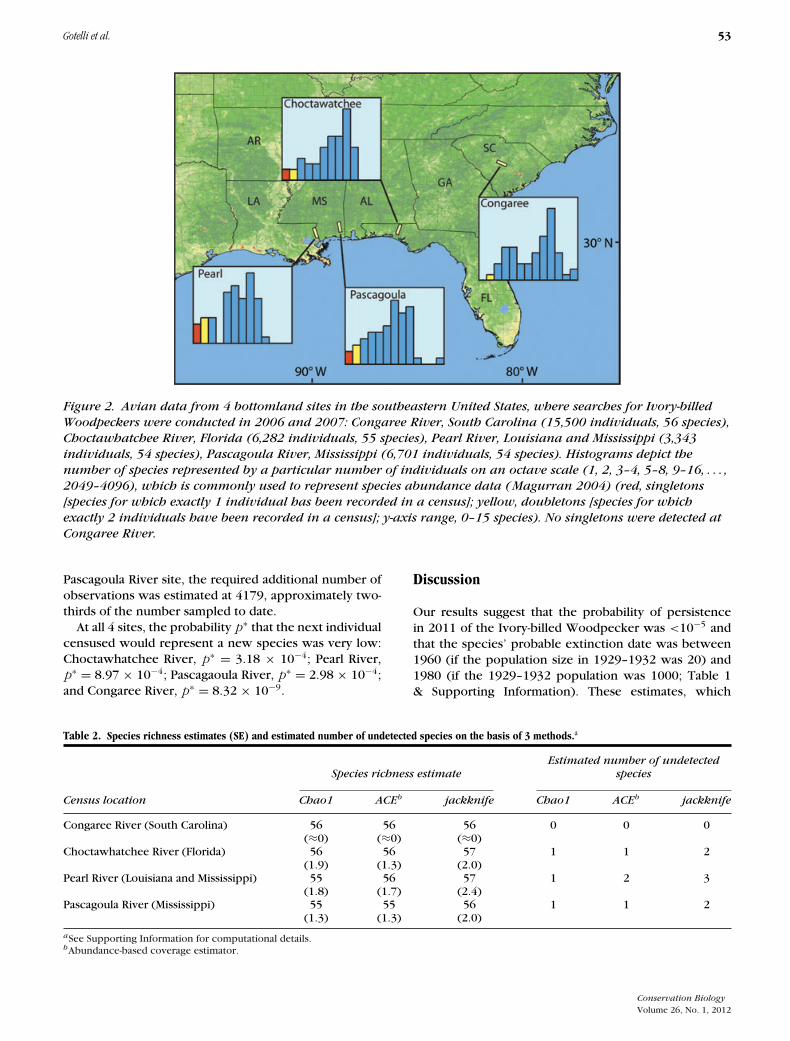
To estimate the number of undetected species at the4 sites, we used 3 species richness estimators that relyon information contained in the frequency distribution ofrare species: Chao1, abundance-based coverage estimator(ACE), and the first-order jackknife (Colwell & Codding-ton 1994; Chao 2005; Supporting Information). To esti-mate the additional sampling effort needed to find theseundetected species, we used equations recently derivedby Chao et al. (2009).

What is the probability p∗ that sampling one additionalindividual in a site will yield a previously undetectedspecies? Turing and Good obtained the first-order approx-imation p∗ ≈ f1

n , which is the proportion of singletons inthe sample of n individuals (Good 1953, 2000). We ex-tended Turing’s formula to apply to samples in which therarest species abundance class is not necessarily the sin-gleton class (Supporting Information). When doubletons(f2) form the rarest abundance class, the probability ofobtaining a previously undetected species is p∗ ≈ 2 f2

n2 .

Results

Specimen-Based Analyses

Our specimen-based model predicted the probabil-ity of persistence of the Ivory-billed Woodpecker in2005–2008, the most recent complete 4-year interval.The estimated number of specimen records between2005 and 2008 was μt = 6.4 × 10−7 (SE = 5.9 × 10−6;Supporting Information). The predicted probability ofpopulation persistence depends on the assumed popu-lation size (N) in 1929–1932. The estimated persistenceprobability ranged from 1.3 × 10−5 for N = 20, to 0.0006for N = 1000, and to 0.0313 for N = 50,000 (Table 1).

On the basis of these probabilities, if we set a per-sistence probability of <0.05 as the criterion of prob-able extinction, the estimated extinction interval forthe Ivory-billed Woodpecker ranged from 1961–1964 forN = 20, to 1969–1972 for N = 100, and to 1981–1984

Table 1. Hypothetical total population sizes of Ivory-billedWoodpeckers from 1929 to 1932, the corresponding predictedprobability of persistence in the time interval 2005 to 2008, and theestimated extinction interval (the earliest period for which theprobability of persistence is <0.05 or <0.01).

Hypothetical Estimated Estimated1929–1932 Probability of extinction extinctionpopulation persistence interval intervalsize 2005–2008 (<0.05) (<0.01)

20 1.3 × 10−5 1961–1964 1969–1972100 6.4 × 10−5 1969–1972 1977–1980500 0.0003 1977–1980 1989–19921,000 0.0006 1981–1984 1993–19965,000 0.0032 1993–1996 2001–200410,000 0.0063 1997–2000 2005–200850,000 0.0313 2005–2008 >2008

for N = 1000 (Table 1 & Supporting Information). Persis-tence later than 2008 was unlikely unless the hypotheticalpopulation size was >50,000 individuals in 1929–1932.With a persistence probability of <0.01 as the criterionfor probable extinction (last column in Table 1), extinc-tion was projected to have occurred in 1969–1972 forN = 20, in 1977–1980 for N = 100, in 1993–1996 forN = 1000, and after 2008 for N = 50,000. Tanner (1942)estimated that approximately 22 woodpeckers were alivein the southeastern United States during the late 1930s.The likelihood that the total population size at this timewas 10,000–50,000 individuals is low. Thus, for a morerealistic population size in 1929–1932 of <100, the es-timated probability of persistence was 6.4 × 10−5 andthe probable extinction date was no later than 1980(Table 1).

Analyses of Contemporary Census Data

According to results of the stopping-rule analysis, thesearch for Ivory-billed Woodpeckers should be halted atthe Congaree River site. After 15,500 observations, therewere no singletons and therefore almost zero probabil-ity of detecting the woodpecker or any other speciesnot already observed that winters regularly in bottom-land hardwood forests at this locality. Surveys at each ofthe other 3 sites have accumulated fewer than half thisnumber of observations, and each of these surveys in-cluded one or more winter-resident species representedby only a single individual (Fig. 2). Because of the largesample sizes used in these surveys, the 3 estimators con-verged to very similar predictions of between 1 and 3undetected species at each of the 3 sites (Table 2 & Sup-porting Information). Estimates of the additional numberof observations needed to find these undetected speciesfor the Choctawhatchee River and Pearl River sites were6613 and 3061 individuals, respectively, about the sameas the number of individuals already sampled. For the

Conservation BiologyVolume 26, No. 1, 2012

Gotelli et al. 53

Figure 2. Avian data from 4 bottomland sites in the southeastern United States, where searches for Ivory-billedWoodpeckers were conducted in 2006 and 2007: Congaree River, South Carolina (15,500 individuals, 56 species),Choctawhatchee River, Florida (6,282 individuals, 55 species), Pearl River, Louisiana and Mississippi (3,343individuals, 54 species), Pascagoula River, Mississippi (6,701 individuals, 54 species). Histograms depict thenumber of species represented by a particular number of individuals on an octave scale (1, 2, 3–4, 5–8, 9–16, . . . ,2049–4096), which is commonly used to represent species abundance data (Magurran 2004) (red, singletons[species for which exactly 1 individual has been recorded in a census]; yellow, doubletons [species for whichexactly 2 individuals have been recorded in a census]; y-axis range, 0–15 species). No singletons were detected atCongaree River.

Pascagoula River site, the required additional number ofobservations was estimated at 4179, approximately two-thirds of the number sampled to date.

At all 4 sites, the probability p∗ that the next individualcensused would represent a new species was very low:Choctawhatchee River, p∗ = 3.18 × 10−4; Pearl River,p∗ = 8.97 × 10−4; Pascagaoula River, p∗ = 2.98 × 10−4;and Congaree River, p∗ = 8.32 × 10−9.

Discussion

Our results suggest that the probability of persistencein 2011 of the Ivory-billed Woodpecker was <10−5 andthat the species’ probable extinction date was between1960 (if the population size in 1929–1932 was 20) and1980 (if the 1929–1932 population was 1000; Table 1& Supporting Information). These estimates, which

Table 2. Species richness estimates (SE) and estimated number of undetected species on the basis of 3 methods.a

Species richness estimateEstimated number of undetected

species

Census location Chao1 ACEb jackknife Chao1 ACEb jackknife

Congaree River (South Carolina) 56 56 56 0 0 0(≈0) (≈0) (≈0)

Choctawhatchee River (Florida) 56 56 57 1 1 2(1.9) (1.3) (2.0)

Pearl River (Louisiana and Mississippi) 55 56 57 1 2 3(1.8) (1.7) (2.4)

Pascagoula River (Mississippi) 55 55 56 1 1 2(1.3) (1.3) (2.0)

aSee Supporting Information for computational details.bAbundance-based coverage estimator.

Conservation BiologyVolume 26, No. 1, 2012

54 Specimen-Based Extinction Assessment

assume a constant search effort, are on the optimisticside because the collective search effort for the Ivory-billed Woodpecker has increased tremendously since1932.

The exhaustive avian censuses carried out to date inthe search for the Ivory-billed Woodpecker (Fig. 2 & Sup-porting Information) also make it unlikely that additionalspecies will be detected at these 4 sites (Table 2) with-out expending almost as much additional effort as hasalready been invested. Of course, even if extensive fur-ther censuses were to yield additional species, there isno guarantee that the Ivory-billed Woodpecker would beamong them. At the Pearl River site, for example, moreplausible candidates for new species observations areAmerican Woodcock (Scolopax minor) and Red-headedWoodpecker (Melanerpes erythrocephalus).

Inevitably, considerable uncertainty must be associ-ated with the statistical estimation of extinction timesfrom historical specimen records. For example, use ofthe Poisson generalized additive model to project spec-imen numbers (Fig. 1) cannot be rigorously justified forapplication to sparse data, and parameter estimates, suchas the size of the Ivory-billed Woodpecker population in1929–1932 (Table 1), can be difficult to establish.

In view of these uncertainties, an effective strategy isto analyze extinction times from a completely differentstatistical perspective and determine whether the resultsare consistent. Elphick et al. (2010) and Roberts et al.(2010) applied Solow’s (1993a, 2005) method, which isderived from extreme value theory, to estimate the ex-tinction year of the Ivory-billed Woodpecker. They basedtheir analyses on physical evidence of museum speci-mens, photographs, and sound recordings as well as onreports of visual sightings confirmed by independent ex-perts. These data were represented as a binary sequenceof annual presences (at least one individual detected inyear t) and absences (no individual detected in year t). El-phick et al. (2010) and Roberts et al. (2010, their Table 2)based their analysis on 39 presences between 1897 and1944, which correspond to the quantitative data usedin our analyses (Supplemental Information) reduced tosimple yearly presence data plus additional records after1932.

In spite of the differing assumptions and treatment ofthe data (discussed fully in Supporting Information), theconclusions of Elphick et al. (2010) and Roberts et al.(2010) are qualitatively consistent with our findings.Their analysis of physical evidence yielded a probableextinction date for the Ivory-billed Woodpecker of 1941,with an upper 95% confidence interval of 1945 (Table 1 inElphick et al. 2010; Fig. 1 in Roberts et al. 2010). Althoughtheir estimated extinction dates differ from ours (1941vs. 1980), our analyses of museum specimens (Fig. 1)and records from contemporary avian censuses (Fig. 2)and the alternative analyses of Roberts et al. (2010)and Elphick et al. (2010) all point to the inescapable

conclusion that the Ivory-billed Woodpecker is nowextinct.

The reported rediscovery of the Ivory-billed Wood-pecker has been one of the most controversial findings inconservation biology, and the survey program designedto confirm that report among the most intensive andcostly. Certainly, such rigorous, quantitative rediscoveryprograms will not be implemented for most possibly ex-tinct species; thus, the methods we used to analyze cen-sus data for the woodpecker cannot be applied often.Similarly, for many species, museum specimen series areeither too meagre or too idiosyncratically obtained (Pyke& Ehrlich 2010) to justify the application of our Poissongeneralized additive model.

Nevertheless, when the data justify it, the analyticalmethods we developed can be applied to other retrospec-tive analyses of museum-collection records and to recordsfrom standardized field surveys, 2 important sources ofdata that are based on evidentiary standards (McKelveyet al. 2008). Moreover, our method can be adapted foruse with Rout et al.’s (2009a, 2009b) analyses of eradica-tion programs for invasive species. These tools can helpguide expectations of search-efforts and optimize the al-location of limited conservation resources in the searchfor other rare species (Chades et al. 2008) or for invasivespecies that have putatively been eradicated (Rout et al.2009a, 2009b).

Acknowledgments

We thank S. Haber and P. Sweet for providing informa-tion on Ivory-billed Woodpecker specimens in the Amer-ican Museum of Natural History, C. Elphick for extensivecomments on the manuscript, and M. Rivadeneira andK. Roy for help in understanding their related work.N.J.G. and R.K.C. were supported by the U.S. National Sci-ence Foundation. A.C. and W.H. were funded by the Tai-wan National Science Council. G.R.G. was supported bythe Alexander Wetmore Fund, Smithsonian Institution,and the Center for Macroecology, Evolution, and Climate,University of Copenhagen. This study is a contribution ofthe Synthetic Macroecological Models of Species Diver-sity Working Group supported by the National Center forEcological Analysis and Synthesis, a Center funded by theNational Science Foundation, the University of California,Santa Barbara, and the State of California.

Supporting Information

The following information is available online: generalstatistical methods for analysis of museum specimendata (Appendix S1); compilation of Ivory-billed Wood-pecker museum specimen data (Appendix S2); statisticalanalyses of Ivory-billed Woodpecker museum specimendata (Appendix S3); statistical analyses of Ivory-billed

Conservation BiologyVolume 26, No. 1, 2012

Gotelli et al. 55

Woodpecker contemporary census data (Appendix S4);comparisons with other published analyses of Ivory-billedWoodpecker extinctions (Appendix S5); frequency dis-tribution of museum specimen data (Appendix S6); fre-quency counts of museum specimen data (AppendixS7); frequency distribution of binned specimen data (Ap-pendix S8); fitted Poisson general additive model (Ap-pendix S9); persistence probabilities as a function ofpopulation size (Appendix S10); frequency counts forcontemporary avian census data (Appendix S11); andspecies counts at each of 4 census sites (Appendix S12).The authors are responsible for the content and func-tionality of these materials. Queries (other than absenceof the material) should be directed to the correspondingauthor.

Literature Cited

Audubon, J. J. 1832. Ornithological biography. E. L. Carey and A. Hart,editors. Philadelphia, Pennsylvania.

Burgman, M. A., R. C. Grimson, and S. Ferson. 1995. Inferring threatfrom scientific collections. Conservation Biology 9:923–928.

Burgman, M., B. Maslin, D. Andrewartha, M. Keatley, C. Boek, and M.McCarthy. 2000. Inferring threat from scientific collections: powertests and an application to Western Australian Acacia species. Pages7–26 in S. Ferson and M. Burgman, editors. Quantitative methodsfor conservation biology. Springer-Verlag, New York.

Chades, I., E. McDonald-Madden, M. A. McCarthy, B. Wintle, M. Linkie,and H. P. Possingham. 2008. When to stop managing or sur-veying cryptic threatened species. Proceedings of the NationalAcademy of Sciences of the United States of America 105:13936–13940.

Chao, A. 2005. Species estimation and applications. Pages 7907–7916 inN. Balakrishnan, C. B. Read, and B. Vidakovic, editors. Encyclopediaof statistical sciences 12. 2nd edition. Wiley, New York.

Chao, A., R. K. Colwell, C.-W. Lin, and N. J. Gotelli. 2009. Sufficient sam-pling for asymptotic minimum species richness estimators. Ecology90:1125–1133.

Collen, B., A. Purvis, and G. M. Mace. 2010. When is a species reallyextinct? Testing extinction inference from a sighting record to in-form conservation assessment. Diversity and Distributions 16:755–764.

Collinson, J. M. 2007. Video analysis of the escape flight of PileatedWoodpecker Dryocopus pileatus: does the Ivory-billed Wood-pecker Campephilus principalis persist in continental North Amer-ica? BMC Biology 5:8.

Colwell, R. K., and J. A. Coddington. 1994. Estimating terrestrial bio-diversity through extrapolation. Philosophical Transactions of theRoyal Society of London Series B: Biological Sciences 345:101–118.

Diamond, J. M. 1987. Extant unless proven extinct? Or, extinct unlessproven extant? Conservation Biology 1:77–79.

Eames, J. C., H. Hla, P. Leimgruber, D. S. Kelly, S. M. Aung, S. Moses, andS. N. Tin. 2005. Priority contribution. The rediscovery of Gurney’sPitta Pitta gurneyi in Myanmar and an estimate of its population sizebased on remaining forest cover. Bird Conservation International15:3–26.

eBird. 2009. An online database of bird distribution and abundance.Avian Knowledge Network and Cornell Laboratory of Ornithology,Ithaca, New York, and National Audubon Society, Washington, D.C.Available from http://www.avianknowledge.net (accessed Decem-ber 2010).

Elphick, C. S., D. L Roberts, and J. M. Reed. 2010. Estimated dates of re-cent extinctions for North American and Hawaiian birds. BiologicalConservation 143:617–624.

Fitzpatrick, J. W., et al. 2005. Ivory-billed Woodpecker (Campephilusprincipalis) persists in continental North America. Science308:1460–1462.

Good, I. J. 1953. The population frequencies of species and the estima-tion of population parameters. Biometrika 40:237–264.

Good, I. J. 2000. Turing’s anticipation of empirical Bayes in connectionwith the cryptanalysis of the naval Enigma. Journal of StatisticalComputation and Simulation 66:101–111.

Hahn, P. 1963. Where is that vanished bird? An index to the knownspecimens of the extinct and near extinct North American species.Royal Ontario Museum, University of Toronto, Toronto.

Hamer, A. J., S. J. Lane, and M. J. Mahony. 2010. Using probabilistic mod-els to investigate the disappearance of a widespread frog-speciescomplex in high-altitude regions of south-eastern Australia. AnimalConservation 13:275–285.

Hasbrouck, E. M. 1891. The present status of the Ivory-billed Wood-pecker (Campephilus principalis). Auk 8:174–186.

Iofescu, M., and P. Tautu. 1973. Stochastic processes and applicationsin biology and medicine. Volume II. Models. Springer-Verlag, Berlin.

Jackson, J. A. 2004. In search of the Ivory-billed Woodpecker. Smithso-nian Institution Press, Washington, D.C.

Magurran, A. E. 2004. Measuring biological diversity. Blackwell Science,Oxford, United Kingdom.

McCarthy, M. A. 1998. Identifying declining and threatened specieswith museum data. Biological Conservation 83:9–17.

McCullagh, P., and J. A. Nelder. 1989. Generalized linear models. 2ndedition. Chapman and Hall/CRC, Boca Raton, Florida.

McKelvey, K. S., K. B. Aubry, and M. K. Schwartz. 2008. Using anecdotaloccurrence data for rare or elusive species: the illusion of reality anda call for evidentiary standards. BioScience 58:549–555.

Pyke, G. H., and P. R. Ehrlich. 2010. Biological collections and ecologi-cal/environmental research: a review, some observations and a lookto the future. Biological Reviews 85:247–266.

Rasmussen, S., and N. Starr. 1979. Optimal and adaptive search for anew species. Journal of American Statistical Association 74:661–667.

Regan, T. J., M. A. McCarthy, P. W. J. Baxter, F. Dane Panetta, and H. P.Possingham. 2006. Optimal eradication: when to stop looking foran invasive plant. Ecology Letters 9:759–766.

Rivadeneira, M. M., G. Hunt, and K. Roy. 2009. The use of sightingrecords to infer species extinctions: an evaluation of different meth-ods. Ecology 90:1291–1300.

Roberts, D. L. 2006. Extinct or possibly extinct? Science 312:997.Roberts, D. L., C. S. Elphick, and J. M. Reed. 2010. Identifying anomalous

reports of putatively extinct species and why it matters. BiologicalConservation 24:189–196.

Roberts, D. L., and A. R. Solow. 2003. When did the dodo becomeextinct? Nature 426:245.

Rohrbaugh, R., M. Lammertink, K. Rosenberg, M. Piorkowski, S. Barker,and K. Levenstein. 2007. 2006–07 Ivory-billed Woodpecker sur-veys and equipment loan program. Report. Cornell Laboratory ofOrnithology, Ithaca, New York. Available from http://www.birds.cornell.edu/ivory/pdf/FinalReportIBWO_071121_TEXT.pdf (acces-sed December 2010).

Rout, T. M., Y. Salomon, and M. A. McCarthy. 2009a. Using sightingrecords to declare eradication of an invasive species. Journal ofApplied Ecology 46:110–117.

Rout, T. M., C. J. Thompson, and M. A. McCarthy. 2009b. Robust deci-sions for declaring eradication of invasive species. Journal of AppliedEcology 46:782–786.

Sibley, D. A., L. R. Bevier, M. A Patten, and C. S. Elphick. 2006. Commenton ‘Ivory-billed Woodpecker (Campephilus principalis) persists incontinental North America. Science Online 311:DOI: 10.1126/sci-ence.1114103.

Conservation BiologyVolume 26, No. 1, 2012

56 Specimen-Based Extinction Assessment

Snyder, N. F. R. 2007. An alternative hypothesis for the cause ofthe Ivory-billed Woodpecker’s decline. Monograph of the WesternFoundation of Vertebrate Zoology 2:1–58.

Snyder, N. F. R., D. E. Brown, and K. B. Clark. 2009. The travails of twowoodpeckers: Ivory-bills and Imperials. University of New MexicoPress, Albuquerque.

Sodhi, N. S., et al. 2008. Correlates of extinction proneness in tropicalangiosperms. Diversity and Distributions 14:1–10.

Solow, A. R. 1993a. Inferring extinction from sighting data. Ecology74:962–964.

Solow, A. R. 1993b. Inferring extinction in a declining population.Journal of Mathematical Biology 32:79–82.

Solow, A. R. 2005. Inferring extinction from a sighting record. Mathe-matical Biosciences 195:47–55.

Solow, A. R., and D. L. Roberts. 2003. A nonparametric testfor extinction based on a sighting record. Ecology 84:1329–1332.

Tanner, J. T. 1942. The Ivory-billed woodpecker. Research report 1.National Audubon Society, New York.

U.S. Fish and Wildlife Service. 2009. Recovery plan for the Ivory-billedWoodpecker (Campephilus principalis). U.S. Fish and Wildlife Ser-vice, Atlanta.

Vogel, R. M., J. R. M. Hosking, C. S. Elphick, D. L. Roberts, and J. M.Reed. 2009. Goodness of fit of probability distributions for sightingsas species approach extinction. Bulletin of Mathematical Biology71:701–719.

Wood, S. N. 2006. Generalized additive models: an introduction withR. Chapman and Hall/CRC Press, Boca Raton, Florida.

Conservation BiologyVolume 26, No. 1, 2012

1

Appendix S1. A general statistical method for estimating the probability of persistence from

museum specimen records

Step 1. The analysis uses museum specimen frequency data in the form of yearly records as in

Appendix S6. Because the raw (yearly) counts typically vary greatly from one year to the next, it

is difficult to model the temporal trend as a smooth curve. Therefore, it will usually be necessary

to first group (bin) the data into multi-year intervals to reveal prominent temporal trends. The

results of the statistical anlaysis are potentially sensitive to the size of the binned interval.

Typically, large intervals (i.e. more data points per bin) lead to a smaller variance but a larger

bias, whereas narrow intervals (fewer data points per bin) lead to a smaller bias but a larger

variance. Appendix S3 demonstrates how to determine an optimal bin size using the Ivory-billed

Woodpecker data as an example.

Step 2. After binning, there are T time-interval bins. Let Yt , t = 1, 2, .., T be the the number of

records for the t-th period, where t =1 is the first binned interval. We first fit a smoothed curve to

the specimen data. If we can assume that the fitted curve of specimen numbers generally reflects

population size pattern, then the fitted series can be used to estimate population abundance.

There are many statistical models can be used to model a time series (and any covariate predictor

variables). We use a generalized additive model (GAM), which combines the properties of

generalized linear models with additive models. The GAM model specifies a distribution

function for Yt (Poisson, normal, binomial etc.) and a link function g, which relates μt = E(Yt) to

the time-varying covariates ,...,2,1;,...,, 21 Ttxxx mttt as:

)(....)()()( 2211 tmmttt xfxfxfg . (S1)

Here “additive” refers to the sum of the functions of f1, f2,…, fm. Each function of f1, f2,…, fm

can be parametric (including linear or quadratic or generalized linear models) or non-parametric

2

(including nonparametric regression). Thus the GAM is flexible and can be fit to many different

kinds of temporal trends. To estimate each f(t), we fit the widely used penalized regression spline

model (Wahba 1990, Ruppert et al. 2006) and selected cubic regression splines as the basis for

constructing each f(t). The penalized regression spline model controls the degree of smoothness

by adding a penalty to the likelihood function. This model usually provides a better fit than

parametric linear or quadratic models. The implementation of the penalized regression spline can

be found in many software applications, including the Proc Glimmix in SAS. A widely used and

free software is the mgcv package in R (Wood, 2006) which can be downloaded from

http://www.r-project.org/. We used Ivory-billed Woodpecker data as an example in Appendix S3

to illustrate the model fitting procedures.

Step 3. After the model fitting, we obtain a fitted time series ,...,2,1;ˆ Ttt. Let k be the latest

time period with non-zero specimen records. That is, after time period k, there are no specimen

records (Yt = 0 for t > k). For a hypothetical population size N in the time interval k, define p as

the probability that any individual would be collected as a specimen within a single time interval.

This probability p in the k-th period can be estimated by the sample proportion Yk/N. We assume

this probability p is a constant in all intervals after time k. Next we estimate the expected

population size in any time interval t > k as kttt YNpn /ˆ/ˆ . The probability of persistence

(of at least one individual) in the t-th interval can be estimated as )0( tnP .

The fitting results in Step 3 can be used to determine an optimal bin size for a particular data set.

For each size interval that is tested, we obtain the fitted series and calculate the adjusted R-

square as a measure of the closeness of the fitted values and the data. The bin size that yields the

largest adjusted R2 from the fitted models is then selected (e.g., a 4-year interval for the Ivory-

3

billed Woodpecker data).

Supplementary Literature Cited

Ruppert, D., Wand, M. P., and R. J. Carroll. 2006. Semiparametric regression. Cambridge

University Press, New York.

Wahba, G. 1990. Smoothing models for observational data. SIAM, Philadelphia.

Wood, S. N. 2006. Generalized additive models: An introduction with R. Chapman and

Hall/CRC Press, Boca Raton.

1

Appendix S2. Compilation of museum specimen data for the Ivory-billed Woodpecker and

historical trends in collecting activity.

Specimen data were compiled from Hahn (1963) with additional data from Jackson (2004) and

Ornis (2004). More than 400 Ivory-billed Woodpecker specimens are deposited in North

American and European museums. Many specimens prepared as taxidermy mounts during the

first half of the 19th

century lack museum labels with date and locality data. However, the quality

of data accompanying specimens collected after 1880 was relatively good because the species

was already considered rare by ornithologists and specimens were highly coveted by museums

and private collectors, both of which placed a premium on well-prepared skins and accurate

locality data.

A substantial proportion of specimens obtained by professional collectors after 1890 were sold

directly to museums and private collectors (Jackson 2004; Snyder et al. 2009). Professional

collectors often employed networks of local hunters to obtain specimens. In the early 1890s,

Arthur T. Wayne, one of the more prolific collectors of Ivory-billed Woodpeckers in Florida, paid

local hunters and trappers up to US$5 ($123 in today’s currency) for specimens in good

condition (Snyder et al. 2009). For comparison, unskilled laborers in rural regions of the

southeastern United States were paid < $1 per day during the 1890s (U.S. Bureau of Labor 1904).

Cash bounties offered by professional collectors and specimen dealers were potent incentives for

local woodsmen to seek out relictual populations. During 1894, specimens were offered for retail

sale at $15 per specimen ($369 in today’s currency; Jackson 2004). Retail valuations of

specimens more than tripled after 1900 as demand greatly outstripped supply (Jackson 2004).

None of the states (Texas, Louisiana, Mississippi, Georgia, Florida, South Carolina) known to

2

support Ivory-billed Woodpecker populations after 1900

(Tanner 1942; Jackson 2004) had laws

protecting the species from commercial collecting in 1903 (Ducher 1903).

Despite the enormous economic incentive, specimen production decreased markedly after 1906

as most of the well-known populations were extirpated. Legal prohibition of commercial

collecting did not occur until the passage of the Migratory Bird Treaty Act of 1918, but effective

regulation of hunting activity of any kind was rare or nonexistent in remote regions of the rural

southeastern United States through the 1930s. State-sanctioned collecting permits for Ivory-

billed Woodpeckers were issued as late as 1932 (Jackson 2004). Populations were also subjected

to intense subsistence hunting and curiosity shooting (Snyder et al. 2009). These sources of

mortality are thought to have greatly outweighed the impact of specimen collecting on relict

populations in the 20th

century (Snyder et al. 2009).

It is likely that the decline of Ivory-billed Woodpecker populations began more than a

millennium ago when American Indian populations expanded greatly in eastern North America

after the introduction of maize cultivation from Mexico. Prized for their bills and plumage, this

species figures frequently in Mississippian culture (800-1500 CE) burial goods, including carved

pipe bowls, shell gorgets, and ceramics (Brain & Phillips 1996; Jackson 2004). Ivory-billed

Woodpecker plumage and bills were traded as curios and ceremonial objects by American

Indians as late as the 19th century, whereas intensive subsistence hunting, trophy hunting, and

scientific collecting by European Americans continued through the early 20th

century (Jackson

2004; Snyder et al. 2009).

3

Range contraction undoubtedly began in earnest with clearing of forests along the lower Atlantic

coastal plain in the Colonial period. The final period of extinction started after the Civil War,

when northern timber companies purchased huge tracts of cheap "government-owned" land in

the southern states. Most virgin timber was cut between 1870 and 1930 (Williams 1989).

Remnant stands lasted until the early 1940s, but the demand for lumber during WW II for gun

stocks, cargo pallets, and plywood for PT boats finished those tracts off (and the woodpeckers

they harbored), including the Singer Tract and another large parcel near Rosedale, Mississippi

(Jackson 2004; Snyder et al. 2009).

In short, the museum specimens on which our analysis is based represent the tail of a long

decline in populations. Our models are based on the premise that the dwindling rate of specimen

accumulation in museum collections mirrors steep population declines throughout the historic

range of the species, particularly given the premium prices paid for specimens by museums and

private collectors after 1880.

Analyses were limited to dated specimens with locality data (at least state). Date refers to the

date of collection rather than the accession date in museums. A few specimens of doubtful

provenance or lacking verifiable dates on museum labels were omitted from the analysis.

Although we only used specimens with reliable locality data, it should be noted that our analyses

are not spatially structured, and instead model the temporal decline of the Ivory-billed

Woodpecker after 1880 throughout its geographic range.

4

Brain, J. P., and P. Phillips. 1996. Shell gorgets. Styles of the late prehistoric and protohistoric

Southeast. Peabody Museum Press, Peabody Museum of Archaeology and Ethnology,

Harvard University, Cambridge.

Supplementary Literature Cited

Dutcher, W. 1903. Report of the A. O. U. committee on the protection of North American birds.

Auk 20:101-159.

Hahn, P. 1963. Where is that vanished bird? An index to the known specimens of the extinct and

near extinct North American species. Royal Ontario Museum, University of Toronto.

Jackson, J. A. 2004. In search of the Ivory-billed Woodpecker. Smithsonian Press, Washington,

D.C.

Ornis. 2004. Ornithological Information System. http://ornisnet.org. Accessed 20 December

2010.

Snyder, N. F. R., D. E. Brown, and K. B. Clark. 2009. The travails of two woodpeckers: Ivory-

bills and Imperials. University of New Mexico Press, Albuquerque.

United States Bureau of Labor. 1904 Wages and hours of labor. Nineteenth Annual Report of the

Commissioner of Labor. Department of Commerce and Labor. Government Printing

Office, Washington, D.C., 976 p.

Williams, M. 1989. Americans and their forests: A historical geography. Cambridge University

Press, Cambridge.

1

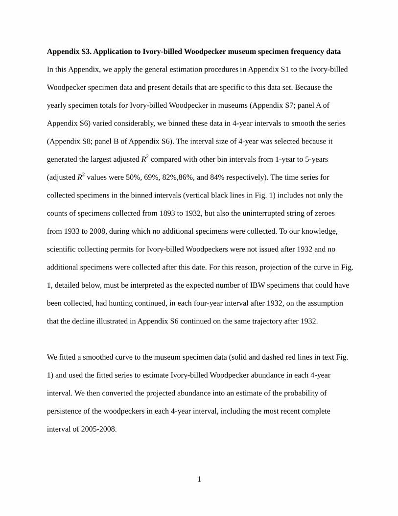
Appendix S3. Application to Ivory-billed Woodpecker museum specimen frequency data

In this Appendix, we apply the general estimation procedures in Appendix S1 to the Ivory-billed

Woodpecker specimen data and present details that are specific to this data set. Because the

yearly specimen totals for Ivory-billed Woodpecker in museums (Appendix S7; panel A of

Appendix S6) varied considerably, we binned these data in 4-year intervals to smooth the series

(Appendix S8; panel B of Appendix S6). The interval size of 4-year was selected because it

generated the largest adjusted R2 compared with other bin intervals from 1-year to 5-years

(adjusted R2

values were 50%, 69%, 82%,86%, and 84% respectively). The time series for

collected specimens in the binned intervals (vertical black lines in Fig. 1) includes not only the

counts of specimens collected from 1893 to 1932, but also the uninterrupted string of zeroes

from 1933 to 2008, during which no additional specimens were collected. To our knowledge,

scientific collecting permits for Ivory-billed Woodpeckers were not issued after 1932 and no

additional specimens were collected after this date. For this reason, projection of the curve in Fig.

1, detailed below, must be interpreted as the expected number of IBW specimens that could have

been collected, had hunting continued, in each four-year interval after 1932, on the assumption

that the decline illustrated in Appendix S6 continued on the same trajectory after 1932.

We fitted a smoothed curve to the museum specimen data (solid and dashed red lines in text Fig.

1) and used the fitted series to estimate Ivory-billed Woodpecker abundance in each 4-year

interval. We then converted the projected abundance into an estimate of the probability of

persistence of the woodpeckers in each 4-year interval, including the most recent complete

interval of 2005-2008.

2

As discussed in the main text, we assume that the decrease in specimens after 1894 reflects a true

decline in Ivory-billed Woodpecker abundance. To model this decline, we assume that Yt

ttYE µ=)(

is a

Poisson random variable with mean where Yt is the number of records for the t-th

four-year period, where t =1 stands for the time period 1893-1896 (the interval with the greatest

number of specimens). We fitted a Poisson GAM to the data after the specimen peak of 1893. In

the model, Yt

log ( )t f tµ α= +

; t = 1, 2, … have different means due to decreasing population size, and the

means are dependent on time. We considered a log link function and the following simple form

of a GAM in Eq. (S1) with time as the sole predictor variable:

, (S2)

where α denotes an unknown baseline constant and f(t) denotes an unknown smooth function of

time. Both α and f(t) are estimated from the data.

We used the mgcv package (Wood 2006) in the R software environment (R Development Core

Team 2008) to carry out the fitting and computation of the penalized regression spline model

(Wahba 1990; Ruppert et al. 2006), We used cubic regression splines (Wahba 1990; Ruppert et al.

2006) to construct a smooth function f(t). For these data, the goodness of fit test yielded a chi-

squared statistic χ2

= 21.95 with 25.7 effective degrees of freedom. From the chi-square

distribution, the P-value = 0.68, implying that the fit of the model to the data was adequate. The

fitted model projects the decline in specimen abundance after 1893 (Fig. 1, Appendix S9) into

more recent time intervals. We focus on inference after 1932 because the last specimen was

collected in that year.

To relate the estimated number of Ivory-billed Woodpecker records in each four-year interval to

3

the corresponding estimated population size, we define p as the probability that any individual,

living woodpeckers would be collected as a specimen or otherwise reliably detected and

recorded within a single, 4-year time interval. Because the last specimen was collected during the

1929-32 interval, and collecting was illegal after 1932, this interval represents the latest

opportunity to infer p from specimen data. Assume the total living population size from 1929-32

is N, then p is approximately 1/N because there was only one specimen collected in this interval.

Thus, we have Np /1≈ in the interval 1929-32. For purposes of the model, we assume that

probability of detection p is roughly a constant after 1932. In fact, the intensity of searches for

Ivory-billed Woodpecker increased substantially after the last known population in Louisiana

disappeared in 1944. If p increased with time, then our analyses over-estimate persistence

probabilities.

Given a hypothetical value of the 1929-32 population size N, we can then estimate the expected

population size of Ivory-billed Woodpeckers in time interval t after 1932 as Npn ttt µµ ˆ/ˆ ≈≈ .

Assuming the population size in any time interval is a Poisson random variable, the probability

of persistence (of at least one individual) in the t-th interval can be estimated as 1 exp( )tn− − ,

which is the probability that a Poisson random variable with mean nt

Supplementary Literature Cited

takes a non-zero value

(Table S4).

R Development Core Team. 2008. R: A language and environment for statistical computing. R

Foundation for Statistical Computing, Vienna.

Ruppert, D., Wand, M. P., and R. J. Carroll. 2006. Semiparametric regression. Cambridge

University Press, New York.

4

Wahba, G. 1990. Smoothing models for observational data. SIAM, Philadelphia.

Wood, S. N. 2006. Generalized additive models: An introduction with R. Chapman and

Hall/CRC Press, Boca Raton.

1

Appendix S4. Statistical analysis of field survey data

Our statistical method for analyzing census data is based principally on the concept of the Good-

Turing frequency formulas (Good 1953, 2000), which helped the British decode German military

ciphers for the Wehrmacht Enigma cryptographic machine during World War II. Alan Turing is

considered to be the founder of modern computer science. His non-intuitive idea (an empirical

Bayesian approach), as applied to the Ivory-billed Woodpecker search problem, is that inference

regarding the probable number of undetected species depends on frequencies of rare species in

the same census area. To apply this concept to our multinomial model for the Ivory-billed

Woodpecker search problem, the species pool considered must be sufficiently large, frequency

data for rare (detected) species must be available, and the sample size should be large.

Ivory-billed Woodpeckers are (or were) conspicuous, diurnal, and sedentary, occupying year-

round territories (Tanner 1942; Jackson 2004). For the purpose of analysis, the pool of species

could be limited appropriately to species that are known to be sedentary, year-round residents of

bottomland forests at the four census sites. We expanded the analyses, however, to include both

resident and migratory species that normally winter in floodplain forest habitats, including early

successional regeneration in canopy gaps. Expanding the sampling pool in this way increases

information about rare species, and therefore potentially increases the estimated number of

undetected species that might be present. We included some species found along roadsides in

bottomland forested habitats (e.g., Mourning Dove) that typically occur in agricultural areas and

old-fields. However, species strongly associated with agriculture and pastures (e.g., Killdeer,

Eastern Meadowlark) were excluded from the analyses. Herons, cormorant, anhinga, ducks, and

coot were excluded, but we included a few species generally associated with rivers and oxbow

2

lakes in bottomland forest (e.g., Bald Eagle, Osprey, Belted Kingfisher, Tree Swallow). Strictly

nocturnal species (e.g., Eastern Screech-Owl) were excluded.

The four sites, searching periods, observed species richness and sample sizes are as follows.

(1) Congaree River, South Carolina: 26 searching days (7 December 2006 to 5 January 2007);

15,500 individuals and 56 species were observed.

(2) Choctawhatchee River, Florida: 14 searching days (23 January 2007 to 7 February 2007);

6282 individuals and 55 species were observed.

(3) Pearl River, Louisiana: 9 searching days (10 February 2007 to 18 February 2007); 3343

individuals and 54 species were observed.

(4) Pascagoula River, Mississippi: 9 searching days (20 February 2007 to 28 February 2007);

6701 individuals and 54 species were observed.

We used a non-parametric approach to estimating species richness based on frequency counts (f1,

f2, …, f10), where fr

denotes the number of species represented by exactly r individuals in sample.

The first ten frequency counts for each site appear in Appendix S11. The detailed data, including

species name and the abundance of each observed species, are provided in Appendix S12.

In the Congaree River site, for example, the ten least common species had observed frequencies

f1 = 0, f2 =1, f3 = 0, f4 =3, f5 =2, …, f10 = 1. That is, there were no singletons, one doubleton, no

species observed three times, three species observed four times, two species observed five

times,…, and one species observed ten times. In the Congaree River census, 13 of 56 species

were relatively rare, observed 10 or fewer times. From a statistical point of view, census data

3

from common species carry almost no information about undetected species; most species

richness estimators are based on inferences derived from the frequency of relatively rare species.

Three estimators of species richness are used in the analysis. All of these estimators converge to

the true species richness, including undetected species, when sample size is sufficiently large.

(1) The Chao1 estimator (Chao 1984)

This estimator is referred to as the Chao1 estimator in the ecological literature (Colwell &

Coddington 1994). This estimator uses only the numbers of singletons and doubletons to

obtain a lower bound of species richness: D is the observed species richness, f1 is the number

of singletons, and f2

is the number of doubletons.

=−+>+

=0if,2/)1(

0 if),2/(ˆ211

222

11 f ffD

f ffDSchao .

(2) ACE (Abundance Coverage-based Estimator; Chao 2005) is based on the first ten

frequencies (f1, f2, …, f10

21 ˆˆˆˆ

rarerarerare

rareabunACE C

fCDDS γ++=

):

,

where Dabun denotes the number of species in the abundant species group (i.e., species with

frequency greater than 10), Drare

−=1ˆrareC

denotes the number of species in the rare species group (i.e.,

species with frequency less than or equal to 10), ∑ =10

11 / i iiff is the estimated

sample coverage in the rare species group, and 2ˆrareγ is the estimated square of CV

4

(coefficient of variation, a measure that characterizes the variation of species abundances) in

the rare group:

−−

−=

∑∑∑

==

= 0,1)1)((

)1(ˆˆ 10

110

1

1012

ififfii

CDmax

i ii i

i i

rare

rarerareγ

(3) The first-order Jackknife estimator (Burnham & Overton 1978) has the following form

1]/)1[(ˆ fnnDSJackknife −+=

That is, only the number of singletons is used to estimate the number of undetected species.

Chao1, ACE, and the Jackknife estimator are easily calculated with the software applications

EstimateS (Colwell 2006) and SPADE (Chao & Shen 2003). The results are shown in Table 2

of the main text.

Turing and Good (Good 1953, 2000) obtained the first-order approximation of the probability P*

nfP /1* ≈

that sampling one additional individual will yield a previously undetected species as ,

which is the proportion of singletons in the sample. With sufficient effort, as additional

individuals are found of species initially represented as singletons, this probability approaches

zero. We have extended Turing’s formula to apply to samples in which the rarest species

abundance class is not necessarily the singleton class. If fr is the expected occurrence frequency

for the rarest abundance class in a sample of n individuals (i.e., fj = 0 for all j < r), then the

approximate probability that the next individual observed will represent a species new to the

survey is

5

rr

nfrP !* ≈ .

Turing’s formula represents the special case of r = 1. For the four census sites, the probabilities

of detecting a new species with the next individual censused are discussed in the main text.

6

Supplementary references

Burnham, K. P. & W. S. Overton. 1978. Estimation of the size of a closed population when

capture probabilities vary among animals Biometrika 65: 625-633.

Chao, A., and T.-J. Shen. 2003. Program SPADE Species Prediction And Diversity Estimation.

User's Guide and application published at:

http://chao.stat.nthu.edu.tw. Accessed 20 December 2010.

Chao, A. 1984. Non-parametric estimation of the number of classes in a population.

Scandinavian Journal of Statistics 11: 265-270.

Chao, A. 2005. Species estimation and applications. Pages 7907-7916 in N. Balakrishnan, C. B.

Read, and B. Vidakovic, editors. Encyclopedia of Statistical Sciences 12. 2nd

Colwell, R. K., and J. A. Coddington. 1994. Estimating terrestrial biodiversity through

extrapolation. Philosophical Transactions of the Royal Society of London B – Biological

Sciences 345: 101–118.

Edition,

Wiley, New York.

Colwell, R.K. 2006. EstimateS: Statistical estimation of species richness and shared species from

samples. Version 8.0. User's Guide and application published

at: http://purl.oclc.org/estimates. Accessed 20 December 2010.

Good, I. J. 1953. The population frequencies of species and the estimation of population

parameters. Biometrika 40: 237–264.

Good, I. J. 2000. Turing’s anticipation of empirical Bayes in connection with the cryptanalysis of

the naval Enigma. Journal of Statistical Computation and Simulation 66: 101–111.

Jackson, J. A. 2004. In search of the Ivory-billed Woodpecker. Smithsonian Press, Washington,

D.C.

7

Tanner, J. T. 1942. “The Ivory-billed Woodpecker. Research Report No. 1” National Audubon

Society, New York.

Appendix S5. Comparisons with other published analyses of Ivory-billed Woodpecker

extinctions.

Solow’s (1993) method is usually interpreted to assume that the total population size remains

constant through time followed by a sudden stochastic extinction (a stationary Poisson process)

(e.g., Solow 2005). In contrast, our quantitative specimen-based analysis assumes that the

diminishing curve of specimen records (Fig. 1 inset) after 1890 reflects a gradual population

decline of the Ivory-billed Woodpecker throughout its geographic range, which would seem to

make the Solow (1993) method inappropriate.

However, an increasing census effort applied to a decreasing population (‘sampling type 4’ with

gradual extinction, in the simulations of Rivadeneira et al. 2009) could, in principle, also yield an

approximately uniform ‘total probability’ of detection up until extinction. Roberts et al. (2010)

justified their application of Solow’s (1993) method on the finding by Vogel et al. (2009, their

Table 2) that data for the populations they considered best fit a uniform distribution of temporal

occurrences, including a data series of 13 ‘undisputed records’ for the Ivory-billed Woodpecker

(an earlier version of the Elphick et al. [2010] dataset, spanning 1897-1939).

However, a potential complication with these analyses is that the crucial terminal sequence of

presence-absence records for the Ivory-billed Woodpecker from 1933 to 1944, analyzed by

Elphick et al. (2010) and Roberts et al. (2010), were all made in a single remnant population that

declined to extinction in northern Louisiana (see Fig. 1; Tanner 1942; Jackson 2004). Moreover,

because the lifespan of an Ivory-billed Woodpecker was probably 10 years or more (U.S. Fish &

Wildlife Service 2009), many of these observations were likely of the same individuals. In

contrast, our specimen-based analysis (Fig. 1) is based on the cumulative database of dated

specimens, each of which can be counted only once, removing at least one key source of non-

independence.

Scott et al. (2008) carried out the only other quantitative analysis of the post-2004 rediscovery

program for Ivory-billed Woodpecker of which we are aware, although they did not use data for

the other species recorded, as we did. Instead, these authors estimated the probability that a

population of n Ivory-billed Woodpeckers could have been present, given the area of

woodpecker habitat covered by the searchers, assuming a spatially uniform probability of

encounter. Unless the population was smaller than 1 or 2 individuals, the search effort was

sufficient to conclude (with P > 0.95) that the Ivory-billed Woodpecker was not present in the

searched area.

Supplementary Literature Cited

Elphick, C. S., D. L Roberts, and J. M. Reed. 2010. Estimated dates of recent extinctions for

North American and Hawaiian birds. Biological Conservation 143: 617–624.

Jackson, J. A. .2004. In search of the Ivory-billed Woodpecker. Smithsonian Press, Washington,

D.C.

Rivadeneira, M. M., G. Hunt, and K. Roy. 2009. The use of sighting records to infer species

extinctions: an evaluation of different methods. Ecology 90: 1291–1300.

Roberts, D. L., C. S. Elphick, and J. M. Reed. 2010. Identifying anomalous reports of putatively

extinct species and why it matters. Biological Conservation 24: 189–196.

Scott, J. M., F. L. Ramsey, M. Lammertink, K.V. Rosenberg, R. Rohrbaugh, J.A. Wiens, and

J.M. Reed. 2008. When is an ‘extinct’ species really extinct? Gauging the search efforts

for Hawaiian forest birds and the Ivory-Billed Woodpecker. Avian Conservation and

Ecology 3: http://www.ace-eco.org/vol3/iss2/art3/

Solow, A. R. 1993. Inferring extinction from sighting data. Ecology 74: 962–964.

Solow, A. R. 2005. Inferring extinction from a sighting record. Mathematical Biosciences 195:

47–55.

Tanner, J. T. 1942. The Ivory-billed woodpecker. Research Report No. 1 National Audubon

Society, New York.

U. S. Fish and Wildlife Service. 2009. Recovery Plan for the Ivory-billed Woodpecker

(Campephilus principalis). U. S. Fish and Wildlife Service, Atlanta.

Vogel, R. M., J. R. M. Hosking, C. S. Elphick, D. L. Roberts, and J. M. Reed. 2009. Goodness of

fit of probability distributions for sightings as species approach extinction. Bulletin of

Mathematical Biology 71: 701–719.

Appendix S6. Dated museum specimens of Ivory-billed Woodpeckers from known

georeferenced localities.

A. Yearly frequency data for museum specimens of the Ivory-billed Woodpecker. B. Museum

specimen data binned in 4-year intervals. Data for the descending portion of collection curve also

appear in Fig. 1 (graph inset).

Appendix S7. Temporal distribution of museum specimens of Ivory-billed Woodpecker

collected in the United States since 1850.

Year Frequency Year Frequency Year Frequency Year Frequency 1850 0 1871 0 1892 2 1913 1 1851 0 1872 1 1893 12 1914 5 1852 0 1873 0 1894 15 1915 0 1853 1 1874 1 1895 3 1916 0 1854 0 1875 0 1896 7 1917 1 1855 0 1876 10 1897 1 1918 0 1856 0 1877 11 1898 5 1919 0 1857 0 1878 2 1899 6 1920 0 1858 0 1879 2 1900 2 1921 0 1859 1 1880 1 1901 3 1922 0 1860 1 1881 6 1902 4 1923 0 1861 0 1882 0 1903 0 1924 0 1862 0 1883 12 1904 21 1925 2 1863 0 1884 3 1905 7 1926 0 1864 0 1885 5 1906 10 1927 0 1865 0 1886 7 1907 4 1928 0 1866 0 1887 14 1908 4 1929 0 1867 0 1888 4 1909 6 1930 0 1868 0 1889 11 1910 1 1931 0 1869 7 1890 5 1911 0 1932 1 1870 3 1891 7 1912 1 >1932 0 Tabled numbers are yearly frequency data (zero means that no museum specimens were collected

that year).

Appendix S8. Binned yearly frequency distribution of museum specimens of the Ivory-billed

Woodpecker.

Period Frequency Period Frequency Period Frequency 1853-56 1 1881-84 21 1909-12 8 1857-60 2 1885-88 30 1913-16 6 1861-64 0 1889-92 25 1917-20 1 1865-68 0 1893-96 37 1921-24 0 1869-72 11 1897-00 14 1925-28 2 1873-76 11 1901-04 28 1929-32 1 1877-80 16 1905-08 25 > 1932 0 Zero means that there were no museum specimens collected in that four-year period. These data

are plotted in Fig. 1 (inset graph) and in Figure S1.

Appendix S9. The Poisson GAM fitted number of Ivory-billed Woodpecker records tµ and the

standard error se( tµ ) in each four-year interval.

Period tµ se( tµ ) Period tµ se( tµ ) 1929-32 0.4225 0.2468 1969-72 0.000375 0.001495 1933-36 0.2157 0.1634 1973-76 0.000184 0.000829 1937-40 0.1078 0.1048 1977-80 9.08×10 0.000457 -5 1941-44 0.0532 0.0657 1981-84 4.47×10 0.00025 -5 1945-48 0.0262 0.0401 1985-88 2.20×10 0.000136 -5 1949-52 0.0129 0.024 1989-92 1.08×10 7.32×10-5 1953-56

-5 0.0064 0.0142 1993-96 5.33×10 3.93×10-6

1957-60

-5 0.0031 0.0082 1997-00 2.62×10 2.10×10-6

1961-64

-5 0.0015 0.0047 2000-04 1.29×10 1.12×10-6

1965-68

-5 8.00×10 0.0027 -4 2005-08 6.36×10 5.94×10-7 -6

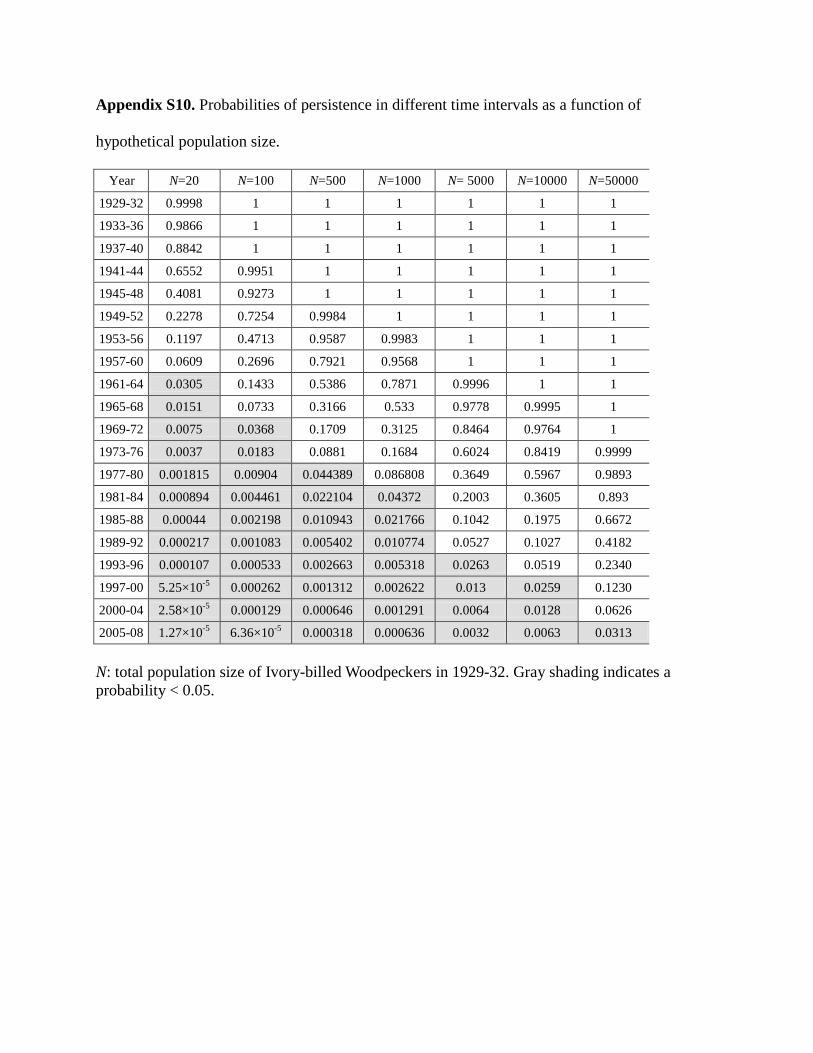
Appendix S10. Probabilities of persistence in different time intervals as a function of

hypothetical population size.

Year N=20 N=100 N=500 N=1000 N= 5000 N=10000 N=50000 1929-32 0.9998 1 1 1 1 1 1 1933-36 0.9866 1 1 1 1 1 1 1937-40 0.8842 1 1 1 1 1 1 1941-44 0.6552 0.9951 1 1 1 1 1 1945-48 0.4081 0.9273 1 1 1 1 1 1949-52 0.2278 0.7254 0.9984 1 1 1 1 1953-56 0.1197 0.4713 0.9587 0.9983 1 1 1 1957-60 0.0609 0.2696 0.7921 0.9568 1 1 1 1961-64 0.0305 0.1433 0.5386 0.7871 0.9996 1 1 1965-68 0.0151 0.0733 0.3166 0.533 0.9778 0.9995 1 1969-72 0.0075 0.0368 0.1709 0.3125 0.8464 0.9764 1 1973-76 0.0037 0.0183 0.0881 0.1684 0.6024 0.8419 0.9999 1977-80 0.001815 0.00904 0.044389 0.086808 0.3649 0.5967 0.9893 1981-84 0.000894 0.004461 0.022104 0.04372 0.2003 0.3605 0.893 1985-88 0.00044 0.002198 0.010943 0.021766 0.1042 0.1975 0.6672 1989-92 0.000217 0.001083 0.005402 0.010774 0.0527 0.1027 0.4182 1993-96 0.000107 0.000533 0.002663 0.005318 0.0263 0.0519 0.2340 1997-00 5.25×10-5 0.000262 0.001312 0.002622 0.013 0.0259 0.1230 2000-04 2.58×10-5 0.000129 0.000646 0.001291 0.0064 0.0128 0.0626 2005-08 1.27×10-5 6.36×10-5 0.000318 0.000636 0.0032 0.0063 0.0313 N: total population size of Ivory-billed Woodpeckers in 1929-32. Gray shading indicates a probability < 0.05.

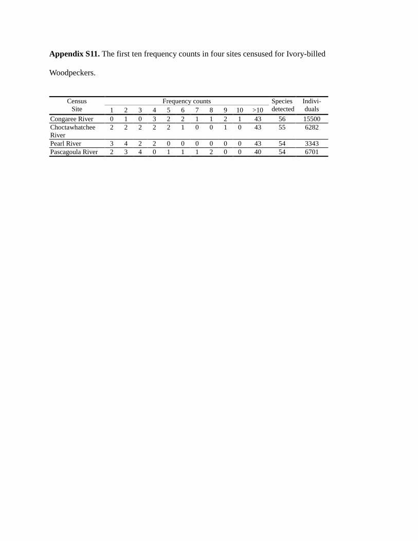
Appendix S11. The first ten frequency counts in four sites censused for Ivory-billed

Woodpeckers.

Census

Site Frequency counts Species

detected Indivi- duals 1 2 3 4 5 6 7 8 9 10 >10

Congaree River 0 1 0 3 2 2 1 1 2 1 43 56 15500 Choctawhatchee River

2 2 2 2 2 1 0 0 1 0 43 55 6282

Pearl River 3 4 2 2 0 0 0 0 0 0 43 54 3343 Pascagoula River 2 3 4 0 1 1 1 2 0 0 40 54 6701

Appendix S12. Avian species and number of individuals censused at four localities in the southeastern United States.

Species

Census locality

Congaree River

Choctawhatchee River

Pascagoula River

Pearl River

Meleagris gallopavo Wild Turkey 93 21 14 1 Coragyps atratus Black Vulture 277 177 31 62 Cathartes aura Turkey Vulture 324 157 147 68 Pandion haliaetus Osprey 0 0 3 2 Haliaeetus leucocephalus Bald Eagle 0 0 1 1

Accipiter striatus Sharp-shinned Hawk 18 3 1 0

Buteo lineatus Red-shouldered Hawk 126 82 88 70

Buteo jamaicensis Red-tailed Hawk 28 9 6 4 Aquila chrysaetos Golden Eagle 2 0 0 0 Falco sparverius American Kestrel 0 1 2 3

Scolopax minor American Woodcock 7 2 5 0

Zenaida macroura Mourning Dove 0 5 3 0 Strix varia Barred Owl 184 96 60 34 Megaceryle alcyon Belted Kingfisher 45 24 43 14 Melanerpes erythrocephalus

Red-headed Woodpecker 9 13 0 0

Melanerpes carolinus Red-bellied Woodpecker 670 498 339 244

Sphyrapicus varius Yellow-bellied Sapsucker 511 390 122 98

Picoides pubescens Downy Woodpecker 344 156 77 75 Picoides villosus Hairy Woodpecker 110 40 32 21 Colaptes auratus Northern Flicker 1100 211 213 204

Dryocopus pileatus Pileated Woodpecker 571 177 216 116

Sayornis phoebe Eastern Phoebe 386 215 63 79 Vireo griseus White-eyed Vireo 10 4 8 2 Vireo solitarius Blue-headed Vireo 101 145 19 11 Cyanocitta cristata Blue Jay 4 63 37 12 Corvus brachyrhynchos American Crow 365 45 37 21 Corvus ossifragus Fish Crow 4 170 92 13 Tachycineta bicolor Tree Swallow 0 5 7 2 Poecile carolinensis Carolina Chickadee 323 138 74 76 Baeolophus bicolor Tufted Titmouse 344 116 46 41 Sitta carolinensis White-breasted 157 0 0 0

Nuthatch

Sitta pusilla Brown-headed Nuthatch 16 0 0 0

Certhia americana Brown Creeper 42 21 11 14 Thryothorus ludovicianus Carolina Wren 309 119 94 57 Troglodytes aedon House Wren 0 6 3 24 Troglodytes troglodytes Winter Wren 394 114 15 21

Regulus satrapa Golden-crowned Kinglet 307 127 27 16

Regulus calendula Ruby-crowned Kinglet 770 435 98 80

Polioptila caerulea Blue-gray Gnatcatcher 9 53 42 45

Sialia sialis Eastern Bluebird 325 29 8 26 Catharus guttatus Hermit Thrush 254 161 44 126 Turdus migratorius American Robin 164 247 169 238 Dumetella carolinensis Gray Catbird 5 1 2 21 Toxostoma rufum Brown Thrasher 8 4 14 16 Bombycilla cedrorum Cedar Waxwing 212 281 150 291

Vermivora celata Orange-crowned Warbler 16 36 22 31

Dendroica coronata Yellow-rumped Warbler 321 453 250 158

Dendroica dominica Yellow-throated Warbler 4 3 0 0

Dendroica pinus Pine Warbler 152 107 12 11

Mniotilta varia Black-and-White Warbler 41 32 3 1

Geothlypis trichas Common Yellowthroat 0 22 33 31

Pipilo erythrophthalmus Eastern Towhee 82 14 19 4 Passerella iliaca Fox Sparrow 6 0 0 3 Melospiza melodia Song Sparrow 15 2 35 55 Melospiza Georgiana Swamp Sparrow 6 57 184 231

Zonotrichia albicollis White-throated Sparrow 639 63 202 220

Junco hyemalis Dark-eyed Junco 164 0 0 2 Cardinalis cardinalis Northern Cardinal 525 235 245 142

Agelaius phoeniceus Red-winged Blackbird 2217 219 3164 66

Euphagus carolinus Rusty Blackbird 28 54 0 37 Quiscalus quiscula Common Grackle 2097 316 2 25 Icterus galbula Baltimore Oriole 5 0 0 0 Carduelis tristis American Goldfinch 254 108 67 77