spread-spectrum methods for lowpass-equivalent volterra
TRANSCRIPT

Spread-Spectrum Methods for
Lowpass-Equivalent Volterra Kernel Identification
in Weakly Nonlinear Passband Systems
Adam R. Wichman
A Dissertation Submitted in Partial Fulfillment of the
Requirements for the Doctor of Philosophy
in the School of Engineering at Brown University
PROVIDENCE, RHODE ISLAND
May 2018

© Copyright 2017 by Adam R. Wichman

This dissertation by Adam R. Wichman is accepted
in its present form by the School of Engineering as satisfying the
dissertation requirement for the degree of Doctor of Philosophy.
DateLawrence E. Larson, Ph.D., Advisor
Recommended to the Graduate Council
DateJacob Rosenstein, Ph.D., Reader
DateDavid Durfee, Ph.D., Reader
Approved by the Graduate Council
DateAndrew G. Campbell, Dean of the Graduate School
iii

Curriculum Vitae
Adam R. Wichman
Research
2013–present
Graduate Research, Brown University, 2015–presentDeveloped novel measurement technique for highly accurate wideband charac-terization of nonlinear microwave systems using spread-spectrum techniques.Developed theory, designed, and prototyped the complete system and demon-strated its effectiveness on RF power amplifiers. SDR system uses commercialcomponents, with time-domain identification method designed for accelerationin real-time applications in place of computationally expensive regression-basedadaptive fitting in existing RF power amplifier digital predistortion systems.Visiting Research Fellow, Fall 2015
National Defense Science and Engineering Graduate Fellow, 2015–present
Graduate Research, Boston University, 2013–2015Designed integrated microwave photonic circuits providing true time delay forW-band phased array communication links, fabricated in LioniX and VTTtechnology. Developed computational models investigating optical generationand carrier transport in GaInAsP (III-V) and HgCdTe (II-VI) short wave in-frared detectors (SWIR); designed novel waveguide unitraveling carrier photo-diodes for increased dynamic range; developed theory explaining dark currentsuppression in densely packed photoarrays; invented new techniques and de-signs to suppress dark current and lateral crosstalk in SWIR focal plane arrays.
College of Engineering, Dean’s Fellow, 2014-2015
Law Practice
2001–2012
Complex civil litigation in patent, antitrust, fraud, contract, environmental disputes,as well as internal investigations, patent prosecution, patent reexamination, intel-lectual property licensing. Supervised case development, expert discovery, motionpractice, depositions.
Law Clerk to Hon. Arthur J. Gajarsa, Circuit Judge,U.S. Court of Appeals for the Federal Circuit, 2004-2005
Law Clerk to Hon. Stephen V. Wilson, District Judge,U.S. District Court for the Central District of California, 2001-2002
iv

U.S. Navy
1992-1997
Division Officer on board USS Boxer (LHD-4), USS Chancellorsville (CG-62); In-structor, Fleet Combat Training Center Pacific;
As a Division Officer led various divisions having from 10 to 60 men as-signed, responsible for sailor welfare, training, professional development,operational readiness and performance; responsible for division equipmentmaintenance and shipyard overhaul.
Service Academy Research Associate, Los Alamos National Laboratory, 1992
Evaluated polarization multiplexed optical communication system; de-signed various electronics in support of evaluations. Awarded electronicssubspecialty code.
EDUCATION EngineeringPh.D., Electrical Engineering, Brown University, expected January 2018.
Dissertation: Spread-Spectrum Methods for Lowpass-Equivalent VolterraKernel Identification in Weakly Nonlinear Passband Sys-tems
Advisor: Lawrence E. Larson
National Defense Science and Engineering Graduate Fellow, 2015–present.
M.S. Electrical Engineering, Boston University, 2014.B.S., Electrical Engineering, with distinction, United States Naval Academy, 1992.
Engineering Duty Option, 1992; Tau Beta Pi, 1991.
OtherJ.D., cum laude, Harvard Law School, 2001.
John M. Olin Fellow in Law and Economics, 2000-2001.
M.Sc. Economics, London School of Economics, 1998.
GRANTS,
HONORS,
& AWARDS
Academic
National Defense Science and Engineering Graduate Fellow, 2015-present.John M. Olin Fellow in Law & Economics, Harvard Law School, 2000-2001.Engineering Duty Option, United States Naval Academy, 1992.Tau Beta Pi, United States Naval Academy, 1991.
Other
Visiting Research Fellow, School of Engineering, Brown University, Fall 2015.Service Academy Research Associate, Los Alamos National Laboratory, 1992.Navy Commendation, Navy Achievement, Southwest Asia Service, and KuwaitiLiberation Medals, Army Airborne.
BAR Massachusetts, California, Washington (inactive)Admitted to various federal district and appellate courts.
v

REGISTRA-
TIONS
U.S. Patent & Trademark Office Reg. No. 43988.Engineer-in-Training, Maryland, 1992.
TECHNICAL ADS, Matlab, Simulink, Python, HDF5, Sentaurus TCAD, Cadence, PhoeniX Op-toDesigner, ASPIC
PUBLICA-
TIONS
Journal Articles
Y. Liu, A. Wichman, B. Isaac, J. Kalkavage, E. Adles, T. Clark, and J. Klamkin,“Ultra-Low Loss Silicon Nitride Optical Beamforming Network for Wideband Wire-less Applications”, IEEE Journal of Selected Topics in Quantum Electronics, 2017(submitted).
Y. Liu, A. Wichman, B. Isaac, J. Kalkavage, E. Adles, T. Clark, and J. Klamkin,“Tuning Optimization of Ring Resonator Delays for Integrated Optical Beam Form-ing Networks,” Journal of Lightwave Technology, vol 35, no. 22, pp. 4954–4960,2017.
J. A. Nanzer,A.Wichman, J. Klamkin, T. P. McKenna, and T. R. Clark, “Millimeter-Wave Photonics for Communications and Phased Arrays,” Fiber and Integrated Op-tics, vol. 34, no. 4, pp.159–174, 2015.
A. R. Wichman, B. J. Pinkie, and E. Bellotti, “Negative Differential Resistance inDense Short Wave Infrared HgCdTe Planar Photodiode Arrays”, IEEE Transactionson Electron Devices, vol. 62, no. 4, pp. 1208-1214, 2015.
A. R. Wichman, B. Pinkie, and E. Bellotti, “Dense Array Effects in SWIR HgCdTePhotodetecting Arrays”, Journal of Electronic Materials, vol. 44, no. 9, pp. 3134–3143, 2015.
R. DeWames, R. Littleton, K. Witte, A. Wichman, and E. Bellotti, “Electro-Optical Characteristics of P+n In0.53Ga0.47As Hetero-Junction Photodiodes in LargeFormat Dense Focal Plane Arrays”, Journal of Electronic Materials, vol. 44, no. 8,pp. 2813–2822, 2015.
B. Pinkie, A. Wichman, and E. Bellotti, “Modulation Transfer Function Conse-quences of Planar Dense Array Geometries in Infrared Focal Plane Arrays”, Journalof Electronic Materials, vol. 44, no. 9, pp. 2981–2989, 2015.
Conference Proceedings
A.R. Wichman, L.E. Larson, “Background Measurement of RF System Nonlinear-ity Using Spread-Spectrum Methods”, 2017 90th ARFTG Microwave MeasurementConference (ARFTG), 2017 (accepted).
Y. Liu, A. Wichman, B. Isaac, J. Kalkavage, E. Adles, T. Clark, and J. Klamkin,“Ring Resonator Based Integrated Optical Beam Forming Network with True TimeDelay for mmW Communications”, 2017 IEEE MTT S International MicrowaveSymposium (IMS), pp. 443-446, 2017.
Y. Liu, A. Wichman, B. Isaac, J. Kalkavage, E. Adles, T. Clark, and J. Klamkin,
vi

“Single ring resonator delays for integrated optical beam forming networks”, 2016IEEE International Topical Meeting on Microwave Photonics, MWP 2016, vol. 7,pp. 321-324, 2016.
Y. Liu, A. Wichman, B. Isaac, J. Kalkavage, E. Adles, and J. Klamkin, 2016.“RingResonator Delay Elements for Integrated Optical Beamforming Networks: GroupDelay Ripple Analysis”. Advanced Photonics 2016 (IPR, NOMA, Sensors, Networks,SPPCom, SOF), OSA technical Digest (online) (Optical Society of America), paperIW1B.3, 2016.
R. DeWames,R. Littleton, K. Witte, A. Wichman, and E. Bellotti,“Modeling DarkCurrent Data of P+n In0.53Ga0.47As Hetero-Junction Photodiodes in Large FormatDense Focal Plane Arrays,” Military Sensing Symposium, 2014.
A. R. Wichman, R. E. DeWames, and E. Bellotti, “Three-dimensional numericalsimulation of planar P+n heterojunction In0.53Ga0.47As photodiodes in dense arraysPart I: dark current dependence on device geometry”, Proc. SPIE 9070, InfraredTechnology and Applications XL 907003, 2014.
A. R. Wichman, R. E. DeWames, and E. Bellotti. 2014. “Three-dimensionalnumerical simulation of planar P+n heterojunction In0.53Ga0.47As photodiodes indense arrays Part II: modulation transfer function modeling”, Proc. SPIE 9070,Infrared Technology and Applications XL 907004, 2014.
In Preparation
A. R. Wichman and L. E. Larson, “A Background Spread-Spectrum Radio Fre-quency Nonlinear Identification Methodology”, 2017.
A. R. Wichman and L. E. Larson, “Spread Pilot Design for Correlation-BasedBandpass Nonlinear Identification”, 2017.
Patent Applications
A. R. Wichman, B. Pinkie, and E. Bellotti, “ Dark Current Mitigation withDiffusion Control.” PCT App. No. US2015/029184 (May 5, 2015), Pub. No.WO2015171572 A1 (Nov 12, 2015) and US 20170077329 A1 (Mar 16, 2017).
vii

Acknowledgements
The opportunity for sustained focus on graduate research in engineering is a luxury
owing the support of many hands. In a sense this particular graduate study started
with my wife’s encouragement, over several years, to go do something interesting.
My fiber optics and waveguides professor at the U.S. Naval Academy, Stephen
Weis, remembered me even many years removed from undergraduate study, and was
willing to support this graduate venture. So did Stephen Burns, my RF electronics
professor and senior design project advisor, now retired in Maine.
Jonathan Klamkin gave me the opportunity to put some knowledge of the GaInAsP
quaternary to work in microwave photonics. We planned to fabricate new waveguide
UTC photodiodes for hybrid integration with silicon-based photonic integrated cir-
cuits. The immediate project, however, was photonic integration providing true time
delay for W band phased array communications. This was a great chance to learn
integrated microwave photonics, optical filter, antenna, and communication system
design, in addition to device design. With Jonathan’s support this led, in part, to
a National Defense Science and Engineering Graduate Fellowship to fund doctoral
studies. I was still helping Jonathan set up the laboratory, to characterize the first
set of true time delay photonic integrated circuits back from the foundry, when the
University of California at Santa Barbara offered him tenure.
Fortunately, within the area, Larry Larson was the Dean for the School of En-
gineering at Brown University. Larry and Jennifer Casasanto were generously open
to, and facilitated, transfer to Brown. The graduate school staff, including Allison
Walsh, Tina Trahan, Kathy DiOrio, and Greg Godino, have at different points all
viii

been helpful with working through details for doing this research. Rachel Levitin, in
the NDSEG program office at ASEE, was instrumental in approving the fellowship
transfer.
While I am not sure how Larry made time to brainstorm ideas, discuss technical
issues, or work through design and prototyping issues for this research, he did. We
set out to try something new on a problem that Larry recognized was significant to
industry, namely, measuring nonlinearity in RF and microwave systems so that we
can proceed to mitigate its unwanted effects. The scope of this research, I think,
kept with the spirit of the NDSEG fellowship to foster independent and creative new
work on practical problems.
Committee members Jacob Rosenstein and David Durfee have also been sounding
boards for different ideas during different stages of this research. Dave has made time
despite the demands of running his own engineering firm, in addition to teaching and
research at Brown.
ix

CONTENTS
Curriculum Vitae iv
Acknowledgments viii
1 Nonlinearity 11.1 Definitions and models . . . . . . . . . . . . . . . . . . . . . . . . . . 2
1.1.1 Linearity . . . . . . . . . . . . . . . . . . . . . . . . . . . . . . 31.1.2 Nonlinearity . . . . . . . . . . . . . . . . . . . . . . . . . . . . 4
1.2 Traditional measures of nonlinearity . . . . . . . . . . . . . . . . . . . 71.2.1 Analytic Taylor series example . . . . . . . . . . . . . . . . . . 81.2.2 Nonlinear model for ideal diode . . . . . . . . . . . . . . . . . 81.2.3 Harmonic stimuli . . . . . . . . . . . . . . . . . . . . . . . . . 10
1.3 Measuring Volterra kernels . . . . . . . . . . . . . . . . . . . . . . . . 121.4 Nonlinearity is the price of power amplifier efficiency . . . . . . . . . 131.5 Memory effects in wideband microwave systems . . . . . . . . . . . . 141.6 Limitations in existing nonlinear measurement . . . . . . . . . . . . . 15
1.6.1 AM/AM, AM/PM models . . . . . . . . . . . . . . . . . . . . 161.6.2 Measuring nonlinearities with a nonlinear vector network an-
alyzer (NVNA) . . . . . . . . . . . . . . . . . . . . . . . . . . 171.6.3 Reducing nonlinearities by predistorting the input with the
nonlinear transfer function inverse . . . . . . . . . . . . . . . . 171.7 A new spread-spectrum measurement approach . . . . . . . . . . . . 18
1.7.1 Early spread-spectrum identification methods . . . . . . . . . 181.7.2 A new spread-spectrum approach. . . . . . . . . . . . . . . . . 201.7.3 Organization . . . . . . . . . . . . . . . . . . . . . . . . . . . 22
2 Spread-Spectrum Methods for Nonlinear Measurement 242.1 Test System Architecture . . . . . . . . . . . . . . . . . . . . . . . . . 252.2 Code design for correlation on intermodulation . . . . . . . . . . . . . 29
2.2.1 Spread pilot design . . . . . . . . . . . . . . . . . . . . . . . . 302.2.2 Nonlinear distortion . . . . . . . . . . . . . . . . . . . . . . . 332.2.3 Intermodulation codes for memoryless cubic nonlinearity . . . 352.2.4 Intermodulation codes for memory representations . . . . . . . 38
x

2.3 Measurement Results . . . . . . . . . . . . . . . . . . . . . . . . . . . 402.3.1 Correlation measurement results . . . . . . . . . . . . . . . . . 432.3.2 Consistent cubic estimates under varying pilot margin . . . . . 492.3.3 Sample memory polynomial coefficients . . . . . . . . . . . . . 52
2.4 Conclusion . . . . . . . . . . . . . . . . . . . . . . . . . . . . . . . . . 53
3 Spread Pilot Design 553.1 Overview . . . . . . . . . . . . . . . . . . . . . . . . . . . . . . . . . . 563.2 Spread pilot design . . . . . . . . . . . . . . . . . . . . . . . . . . . . 56
3.2.1 Stimulating the nonlinearity by the operating signal . . . . . . 563.2.2 Designing pilots for nonlinear measurements . . . . . . . . . . 593.2.3 Code acquisition . . . . . . . . . . . . . . . . . . . . . . . . . 77
3.3 Conclusion . . . . . . . . . . . . . . . . . . . . . . . . . . . . . . . . . 83
4 Conclusion 854.1 Comparison to other nonlinear measurement approaches . . . . . . . 854.2 Future directions for this research . . . . . . . . . . . . . . . . . . . . 88
4.2.1 Acceleration in FPGA, DSP, SoC, or ASIC . . . . . . . . . . . 884.2.2 Extend measurement parameters . . . . . . . . . . . . . . . . 894.2.3 Measure the distortion kernels for spectral broadening . . . . . 904.2.4 Device characterization . . . . . . . . . . . . . . . . . . . . . . 904.2.5 Ultrawideband systems . . . . . . . . . . . . . . . . . . . . . . 904.2.6 Novel system design . . . . . . . . . . . . . . . . . . . . . . . 914.2.7 Calibration . . . . . . . . . . . . . . . . . . . . . . . . . . . . 914.2.8 Predistortion . . . . . . . . . . . . . . . . . . . . . . . . . . . 914.2.9 Novel memory polynomials . . . . . . . . . . . . . . . . . . . . 914.2.10 Optical systems . . . . . . . . . . . . . . . . . . . . . . . . . . 924.2.11 Nonlinear theory . . . . . . . . . . . . . . . . . . . . . . . . . 92
A Definition of Terms 101
B AM/AM, AM/PM Model and the Volterra Series 106B.1 Memoryless Volterra kernel . . . . . . . . . . . . . . . . . . . . . . . . 107B.2 Relation to AM/AM, AM/PM model . . . . . . . . . . . . . . . . . . 108
C Direct Sequence Spread-Spectrum 111C.1 Signal model . . . . . . . . . . . . . . . . . . . . . . . . . . . . . . . . 111C.2 Processing gain . . . . . . . . . . . . . . . . . . . . . . . . . . . . . . 111
C.2.1 Signal . . . . . . . . . . . . . . . . . . . . . . . . . . . . . . . 112C.2.2 Jammer . . . . . . . . . . . . . . . . . . . . . . . . . . . . . . 112C.2.3 Correlation . . . . . . . . . . . . . . . . . . . . . . . . . . . . 113
D Volterra Frequency Representations 116D.1 Volterra model . . . . . . . . . . . . . . . . . . . . . . . . . . . . . . 116D.2 Relations between time, frequency, and multidimensional Volterra rep-
resentations . . . . . . . . . . . . . . . . . . . . . . . . . . . . . . . . 117
xi

D.3 Application to cubic distortion and spread pilots . . . . . . . . . . . . 119
E Generalized Multitone Analysis 124E.1 Generalized multitone analysis . . . . . . . . . . . . . . . . . . . . . . 124E.2 Cubic distortion . . . . . . . . . . . . . . . . . . . . . . . . . . . . . . 126
F Exemplary In-Band Cubic Kernel Measurement 130
G Calibration 135G.1 An Ideal Nonlinear Reference . . . . . . . . . . . . . . . . . . . . . . 135G.2 Shunt Diode Reference . . . . . . . . . . . . . . . . . . . . . . . . . . 138G.3 Other Calibration Options . . . . . . . . . . . . . . . . . . . . . . . . 139
H Testbed Components 141
I Publications 142I.1 Graduate research: Integrated Microwave Photonics . . . . . . . . . . 142I.2 Graduate research: SWIR Devices . . . . . . . . . . . . . . . . . . . . 143
xii
LIST OF TABLES
1.1 Spread-spectrum nonlinear measurement. . . . . . . . . . . . . . . . . 21
2.1 Third-order distortion terms. . . . . . . . . . . . . . . . . . . . . . . . 362.2 CPT Intermodulation. . . . . . . . . . . . . . . . . . . . . . . . . . . 362.3 Intermodulation Codes. . . . . . . . . . . . . . . . . . . . . . . . . . . 372.4 CPT expansion for Generalized Memory Polynomial intermodulation
codes. . . . . . . . . . . . . . . . . . . . . . . . . . . . . . . . . . . . 392.5 Measured linear coefficients. . . . . . . . . . . . . . . . . . . . . . . . 442.6 Reference pilot PN amplitude A given pilot margin PM. The compos-
ite test signal s(t) has PAPR ∼ 11 − 13 dB. DAC full-scale range is±1V . . . . . . . . . . . . . . . . . . . . . . . . . . . . . . . . . . . . . 48
2.7 Measured Diagonal Memory Polynomial Kernels . . . . . . . . . . . . 52
3.1 Third-order distortion terms. . . . . . . . . . . . . . . . . . . . . . . . 623.2 Single pilot cubic intermodulation codes. . . . . . . . . . . . . . . . . 643.3 Cubic intermodulation codes by distortion type. . . . . . . . . . . . . 683.4 LFSR States For r = 3 m-sequence. . . . . . . . . . . . . . . . . . . . 723.5 Product State Matrix and Product Shift Vector. . . . . . . . . . . . . 73
4.1 Spread-spectrum nonlinear measurement. . . . . . . . . . . . . . . . . 86
E.1 Third-Order Distortion Terms . . . . . . . . . . . . . . . . . . . . . . 128
F.1 Third-order lowpass-equivalent Volterra kernel estimates. . . . . . . . 130
G.1 Nonlinear Reference Circuits. . . . . . . . . . . . . . . . . . . . . . . 136
H.1 Principle testbed components. . . . . . . . . . . . . . . . . . . . . . . 141
xiii

LIST OF FIGURES
2.1 Signal path with baseband test signal s(t) generated from multiplexed
pilots x(t) added to the operating signal ˜η(t). . . . . . . . . . . . . . 262.2 Spectrum of baseband test signal pilots X(ω) arrayed in multiple chan-
nels spanning the operating signal η(ω). . . . . . . . . . . . . . . . . 272.3 Diagram of nonlinear test system. The transfer switch provides a
“through” calibration for the linearity measurement. . . . . . . . . . 282.4 m-channel envelope recovery and code acquisition. . . . . . . . . . . 282.5 Correlations on m channel received signal Im or Qm, against unique
real (ICIq ) or quadrature (ICQ
q ) intermodulation codes, measure theparticular q nonlinear distortion coefficient associated with the distor-tion in that channel. Each correlation separates a unique distortionterm. . . . . . . . . . . . . . . . . . . . . . . . . . . . . . . . . . . . 29
2.6 CPT detail. (a) CPT constellation, (b) Normalized pseudoternary(PT) autocorrelation ⟨a1, a1⟩ . . . . . . . . . . . . . . . . . . . . . . 31
2.7 Measured baseband response for linear and DUT signal paths at PM9 dB. . . . . . . . . . . . . . . . . . . . . . . . . . . . . . . . . . . . . 40
2.8 Measured first-zone intermodulated distortion envelope for test signalcomprising five CPT pilots spanning 10 MHz offset (5 MHz baseband)spectrum as shown for the operating signal of interest in Figs. 2.7 and2.2. Fig. 2.8a shows the measured linear testbed response to a com-posite CPT-only test signal. A small DC component is added to eachpilot. The DC component is visible as a frequency impulse at thecenter of each multiplexed CPT pilot and associated test signal sam-pling channel, labeled A to E. Fig. 2.8b shows the measured distortionenvelope spectrum for the stimulus in Fig. 2.8a with pilot intermodu-lation including third-order (5 to 15 MHz) and fifth-order (5-25 MHz)spectral broadening within the first zone. The (intermodulated) DCcomponents provide frequency impulses marking the center of eachpotential sampling channel in the resulting intermodulated distortionenvelope, with the visible upper spectral broadening labeled F to O. . 42
2.9 Measured complex linear transfer coefficient components for morethan 50 dwells after code alignment on center channel with 1960 MHzLO. Shaded region marks calibration interval routing signal throughlinear path on testbed. . . . . . . . . . . . . . . . . . . . . . . . . . . 44
xiv

2.10 Measured uncalibrated correlation output for in-phase and quadra-ture cubic kernel estimates z31(−2, 0, 0) and z32(−2, 0, 0) at 9 dB pilotmargin. Each dwell marks an independent measurement across thefull PN sequence. The shaded region in each plot shows the linearcalibration phase. . . . . . . . . . . . . . . . . . . . . . . . . . . . . . 50
2.11 Uncalibrated mean lowpass-equivalent SMD3 and XMD3 distortionkernel magnitude estimates (in arbitrary units) with fLO = 1960 MHz. 50
2.12 Measured uncalibrated nonlinear correlated output z vs. PN pilot am-plitudes for f = [−2, 0, 0] (corresponding to third-order cross-modulationat -2 MHz due to the pilot at 0 MHz). Overlapping markers for eachPM case show correlations measured at 43 dwells. . . . . . . . . . . . 51
2.13 Measured uncalibrated correlation output z (normalized by channelamplitudes) as a function of pilot margins. Below 9 dB pilot margin
for this case, the value represents an uncalibrated estimate of |h−2,0,031 +
jh−2,0,032 |. . . . . . . . . . . . . . . . . . . . . . . . . . . . . . . . . . . 51
2.14 Memory polynomial estimates at Rc 1 MHz using shunt Schottkydiode at 200 mA forward bias as nonlinear calibration reference. . . . 52
3.1 Test signal S design given operating signal η modeled as bandlim-ited Gaussian white noise, and pilots X =
∑i Aixi: (a) baseband
test signal generation and injection at DUT, showing cubic distortionenvelope; (b) test signal envelope detail, with dashed lines markingchannels associated with each pilot. [From [84].] . . . . . . . . . . . . 58
3.2 Intermodulation code triplet generation. S is the code space size N =2r−1 forQ CPT pilots from primitive polynomial degree r over GF(2).A1 is the set of m-sequences used in all Q CPT pilots, A2 ⊂ A1 is theset of m-sequences used for linear kernel extraction. B is the set ofintermodulated code terms in the DUT output envelope excluding thecorrelated linear codes from the SMD3 and XMD3 distortions (e.g.,i = j, k = i, j), so that A = A1 ∪ B is the set of m-sequences inthe DUT output envelope. C ⊂ B is the set of intermodulated codetriplets in the DUT output envelope selected as correlation argumentsfor cubic distortion kernel identification. . . . . . . . . . . . . . . . . 71
3.3 Pseudoternary sequence normalized periodic autocorrelation. . . . . . 783.4 Offset spectrum for orthogonal pulse-shaped CPT pilots X(f) with
chip rate Rc = 1 MHz in baseband at −4, 2, 0, 2, 4 MHz with B = 5MHz bandlimited operating signal η(f) at 20 dB pilot margin. Dashedlines mark the central (zero offset) channel. (Compare Fig. 3.1.) . . . 79
3.5 Measured code acquisition for r = 20, channel 3 of 5, with pilot margin20 dB. Accumulated phase is nearly an integer multiple of π. . . . . . 82
3.6 Measured code acquisition for r = 20, channel 2 of 5. Accumulatedphase is nearly an integer multiple of π
2. . . . . . . . . . . . . . . . . 83
D.1 Cubic frequency volume corresponding to H(ωi, ωj,−ωk) with spread
pilots Xq(ωq), q ∈ (i, j, k). . . . . . . . . . . . . . . . . . . . . . . . . 122
G.1 Nonlinear reference circuit using shunt Schottky diode. (a) circuitmodel; (b) component placement . . . . . . . . . . . . . . . . . . . . 138
xv
CHAPTER One
Nonlinearity
This work develops novel methods for measuring the lowpass-equivalent nonlinear
transfer coefficients in a truncated Volterra series representing weakly nonlinear ra-
dio frequency (RF) or microwave systems or devices. Measuring the frequency-
dependent polynomial coefficients in these behavioral models is notoriously difficult,
in part because it varies with frequency, dc bias, signal level and history. Pre-
vailing measurement methods are significantly limited because they rely on mea-
suring nonlinearities using unrepresentative signals in a laboratory environment, or
regressions on in situ stimulus and response measurements that are often poorly
conditioned. The approach presented in this work addresses limitations in the pre-
vailing microwave and RF system identification methodologies, drawing on results
and tools from several distinct fields including spread-spectrum communications,
algebraic coding theory, Volterra theory, distortion theory, and nonlinear system
identification.
In the novel approach direct sequence spread-spectrum coding provides pilots that
are combined, in the digital baseband, with uncorrelated wideband operating signals.
The operating signal stimulates a nonlinearity that systematically intermodulates the
relatively low-power spread pilots. The output from a device under test carries a
1

distortion envelope that includes contributions from intermodulated spread coding.
Correlating the envelope, on a channel basis, against intermodulated coding uniquely
associated with each distortion term measures the Volterra kernel for that particular
distortion.
The methodology developed in this work measures the nonlinear transfer function
at several points in multidimensional frequency space. This resembles the rich pa-
rameterization results available from commercially available multisine measurement
approaches, but is instead measured during actual device operation, with the device
nonlinearity stimulated by actual operating signals and subject to in situ loads and
electric and thermal bias.
While regressions on stimulus and response measurements can also estimate ker-
nels with nonlinearities stimulated by actual operating signals under actual operating
conditions, the Volterra kernels are not orthogonal. These regressions, as a result,
can require inverting poorly conditioned matrices, resulting in wide error bounds
on parameter estimates that are not reduced by increasing the number of samples.
The proposed measurement precision, by contrast, is limited by process gain. The
new method thus avoids the conditioning problems associated with traditional kernel
identification involving regressions on stimulus and response measures.
1.1 Definitions and models
Mild nonlinearities with memory are often represented with a polynomial specified
by Volterra kernels or coefficients in a truncated Volterra series, which can be re-
garded as a Taylor series with memory [1], and understood by comparison to the
linear time-invariant (LTI) convolution and impulse response. Nonlinear identifi-
cation means accurately measuring (estimating) the relevant Volterra kernels that
define the nonlinearity over the necessary range of frequencies and operating condi-
tions.
2

The Volterra polynomial representation has been used to describe broad classes
of weakly nonlinear systems (smooth nonlinearities). The Volterra representation,
however, tends to require high-order polynomials to describe hard nonlinearities,
resulting in a rapid growth in model parameters [2, 3]. Other models and techniques,
including describing functions, radial basis functions, or neural networks, have been
used to describe such nonlinearities. This work focuses attention on polynomial
representations for the weakly nonlinear systems generally addressed by a low-order
Volterra series.
1.1.1 Linearity
A linear system y(t) = H[x(t)] with operator H[·] satisfies superposition,
y(t) = H[a1x1(t) + a2x2(t)] (1.1)
= a1H[x1(t)] + a2H[x2(t)].
For a single-input x(t), single-output y(t), the stationary causal linear system is
described by the convolution
y(t) =
∫ ∞
∞h(τ)x(t− τ)dτ (1.2)
=
∫ ∞
∞h(t− τ)x(τ)dτ
with the kernel or impulse response h(t) = 0, t < 0. The usual assumption is that
the impulse response is real-valued and piecewise continuous over all time, allowing
impulses at t = 0 [1], although it is straightforward to extend the recitation using
real or complex discrete time sequences and coefficients [4]. The system has fading
memory if h(τ) → 0 as τ → ∞ [5]. The system has finite memory T if h(τ) = 0 for
τ > T . In a causal system, “memory” describes the set of past stimuli that affect
3

the instant response, through the applicable limits on the convolution.
The more general nonstationary linear system can be described by
y(t) =
∫ ∞
∞h(t, τ)x(τ)dτ (1.3)
with h(t, τ) = 0, τ > t with h(t, τ) piecewise continuous on t ≥ τ ≥ 0, and the
stationary kernel g(t) a special case such that g(t − τ) = h(t, τ). The impulse
response h(t, τ) characterizes the system [1].
1.1.2 Nonlinearity
A stationary (time-invariant), causal, real-valued function (nonlinear system opera-
tor) H[·] of n variables hn(t1, . . . , tn), with hn(t1, . . . , tn) = 0 for any ti < 0, i ∈ [1, n],
can be described by generalizing (1.2),
y(t) =
∫ ∞
∞. . .
∫ ∞
∞hn(τ1, . . . , τn)x(t− τ1) . . . x(t− τn)dτ1 . . . dτn (1.4)
=
∫ ∞
∞. . .
∫ ∞
∞hn(t− τ1, . . . , t− τn)x(τ1) . . . x(τn)dτ1 . . . dτn.
The degree-n homogenous nonlinear system in (1.4) obviously violates superposition
(1.1) for scalar α with H[αx(t)] = αnH[x(t)].
A related, time-invariant nonlinear representation is the Volterra series. The
Volterra series relies on the proposition that “every functional G[x] that is continuous
in the field of continuous functions can be represented by the expansion”
G[x] =∞∑n=0
Fn[x] (1.5)
with each Fn[x] “a regular homogenous functional” of the form in (1.4) [6].
The Volterra series provides exact representation of nonlinear operators, subject
to convergence conditions that we assume for purposes of this work are satisfied by
4

weakly nonlinear systems [1, 5, 7, 8]. Rewriting (1.5), and discarding the DC (zero
stimulus) response (n = 0), the Volterra series has the general form
y(t) = H[x(t)] =∞∑n=1
yn(t), (1.6a)
yn(t) =
∫ ∞
−∞. . .
∫ ∞
−∞hn(τ1, . . . , τn)
n∏i=1
x(t− τi)dτi. (1.6b)
As with (1.4), for a causal system hn(τ1, . . . , τn) = 0 if any τi < 0, i ∈ [1, n]. The
Volterra coefficient hn is called the nth-order kernel. The first-order Volterra series
(n = 1) provides the well-known LTI system response (1.2). The Volterra series
(1.6a) has an infinite number of kernels hn, which makes it somewhat cumbersome
to estimate or manipulate. In practice the Volterra series (1.6) is approximated by
a truncation, such as keeping terms to order n = N as an estimate of nonlinear
operator H[·] [5].
If we regard a nonlinear operator H[·] = (F G)[·] as the response of nonlinearity
G[·] convolved with an ideal first-zone bandpass filter F [·], then we can express
the Volterra series in (1.6) to nonlinear order N in the baseband in terms of an
output signal envelope y(t), input signal envelope x(t), and complex-valued lowpass-
equivalent Volterra kernels hn(·), as [9–11]
y(t) = H[x(t)] =
⌈N2⌉−1∑
k=0
y2k+1(t), (1.7a)
y2k+1(t) =
∫ ∞
0
. . .
∫ ∞
0
h2k+1(τ1, . . . , τ2k+1) (1.7b)
×k+1∏i=1
x(t− τi)2k+1∏i=k+2
x∗(t− τi)(dτ1 . . . dτ2k+1)
with ⌈·⌉ the ceiling operator. This representation facilitates digital baseband analysis
and signal manipulation.
Memory depth in the nonlinear Volterra series is more subtle than in the LTI
5
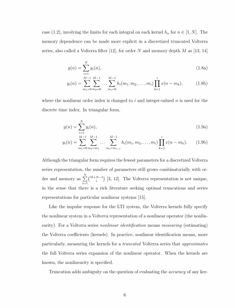
case (1.2), involving the limits for each integral on each kernel hn for n ∈ [1, N ]. The
memory dependence can be made more explicit in a discretized truncated Volterra
series, also called a Volterra filter [12], for order N and memory depth M as [13, 14]
y(n) =N∑i=1
yi(n), (1.8a)
yi(n) =M−1∑m1=0
M−1∑m2=0
. . .
M−1∑mi=0
hi(m1,m2, . . . ,mi)i∏
k=1
x(n−mk), (1.8b)
where the nonlinear order index is changed to i and integer-valued n is used for the
discrete time index. In triangular form,
y(n) =N∑i=1
yi(n), (1.9a)
yi(n) =M−1∑m1=0
M−1∑m2=m1
. . .M−1∑
mi=mi−1
hi(m1,m2, . . . ,mi)i∏
k=1
x(n−mk). (1.9b)
Although the triangular form requires the fewest parameters for a discretized Volterra
series representation, the number of parameters still grows combinatorially with or-
der and memory asN∑i=1
(M+N−1
i
)[3, 12]. The Volterra representation is not unique,
in the sense that there is a rich literature seeking optimal truncations and series
representations for particular nonlinear systems [15].
Like the impulse response for the LTI system, the Volterra kernels fully specify
the nonlinear system in a Volterra representation of a nonlinear operator (the nonlin-
earity). For a Volterra series nonlinear identification means measuring (estimating)
the Volterra coefficients (kernels). In practice, nonlinear identification means, more
particularly, measuring the kernels for a truncated Volterra series that approximates
the full Volterra series expansion of the nonlinear operator. When the kernels are
known, the nonlinearity is specified.
Truncation adds ambiguity on the question of evaluating the accuracy of any ker-
6

nel estimate from a nonlinear identification. Accuracy depends on both statistical
variability and systematic error. Estimating parameters for a truncation that only
poorly approximates a nonlinearity will cause systematic error; with poor condition-
ing this can add statistical variability as well. The kernel estimates, in other words,
may be quite precise, but wholly inaccurate because the truncated Volterra series is
not representative.
The model specification can proceed by assumptions drawn from physical or
sparsity relations, or can be identified through adaptive parameter estimation [16].
“A system identification method is only as good as the model it utilizes.” [17].
In general the model selection is driven by efforts to reduce the parameter space
dimensions [15, 16, 18]. In this context nonlinear identification measures the Volterra
kernels, for a nonlinear device under test (DUT), subject to a preselected series
truncation or representation (or an adaptive model).1
1.2 Traditional measures of nonlinearity
The typical microwave power amplifier data sheet reports nonlinearity in terms of
much coarser metrics like input or output-referred third-order intercept point, or IP3.
Higher IP3 means the device is ‘more linear’—a somewhat imprecise identification
or measure of nonlinearity compared to the parameterized Volterra series. This sim-
plification relates to a special case Volterra series with harmonic stimulus, truncated
(or at least investigated) to third-order (N = 3). With a memoryless approximation
this can be used as reasonably accurate representations for narrowband systems and
devices, but fails as system bandwidth increases.
1Determining the nonlinear order and memory depth can depend on several considerations includingthe analytic, physical or behavioral basis for the model, and may also include the identificationmethodology [12, 15].
7

1.2.1 Analytic Taylor series example
Start by assuming a real, memoryless nonlinearity: hn(τ1, . . . , τm) = 0 ∀τi = 0, i ∈
[1,m]. Applying these simplifications to (1.6), we can write y(t) = F [x(t)], which we
can expand around a given device operating point as
y(t) = h1x(t) + h2x(t)2 + h3x(t)
3 + . . . . (1.10)
Treating (1.10) as a Taylor (Maclaurin) series expansion around x(t) (with (1.10)
converging to F [x(t)]), then we can observe [19]
h1 =dF
dx(1.11a)
h2 =1
2!
d2F
dx2(1.11b)
h3 =1
3!
d3F
dx3. (1.11c)
For an analytic nonlinear functional these kernels can be evaluated symbolically.
1.2.2 Nonlinear model for ideal diode
By way of example, suppose we take a diode in forward bias at DC current Id and
small-signal current id(t) with an ideal diode relation
i(t) = Id + id(t) = Isexp
(Vd + vd(t)
n0VT
+ 1
)(1.12)
where Vd is the DC bias voltage, vd(t) is the small-signal voltage, and DC bias current
Id = Isexp
(Vd
n0VT
+ 1
)(1.13)
8

with n0 the ideality factor and VT = kBTq. Then
id ≃ Isexp
(vd(t)
n0VT
). (1.14)
We can write (1.10) in terms of this diode relation as
id ≃ g1vd(t) + g2v2d(t) + g3v
3d(t) (1.15)
with
n!gn =∂nid(t)
∂v(t)n
∣∣∣∣Id
(1.16)
and
gn =1
n!
(1
n0VT
)n
Id. (1.17)
Using (1.10) we observe that gn = hn, n ∈ [1, 3] in units of A/Vn and
id(t) ≃ Id
(1 +
(1
n0VT
)vd(t) +
12
(1
n0VT
)2vd(t)
2 + 16
(1
n0VT
)3vd(t)
3
). (1.18)
By inspection the ratio of the diode third-order kernel to the first-order kernel has
an analytic expression in terms of device fundamentals,
h3
h1
=1
6
(1
n0VT
)2
(1.19)
in
(1
V2
).
By inspection even this simple example makes some general points about the
nonlinear kernels. Within the limits of the device model, the kernels depend, in this
case, on the current bias point. When expressed in terms of device fundamentals
9

these kernels also have a clear dependence on temperature T−n. In other words, the
nonlinearity is defined by reference to a particular electrical and thermal operating
point.
1.2.3 Harmonic stimuli
We can express basic data sheet nonlinearity measures in terms of the kernels in a
memoryless third-order Volterra series. For a single tone harmonic stimuli, x(t) =
A1cos(ω1t+ α1). Substituting for x(t) in (1.10) [19, 20],
y(t) = A1h1cos(ω1t+ α1)+ (1.20)
A21h2
(12+ cos(2ω1t+ 2α1)
)+
A31h3
(34cos(ω1t+ α1) +
14cos(3ω1t+ 3α1)
).
In the first zone (at ω1) the distorted signal is
(A1h1 +
34A3
1h3
)cos(ω1t+ α1). The
first-zone cubic distortion can be expansive (h1h3 > 0) or compressive (h1h3 < 0) for
large signal x(t) [20]. This gives an input 1 dB compression point at peak amplitude
A1dB =(√
0.145∣∣h1/h3
∣∣) [20]. For a weak nonlinearity (ignoring the signal at the
third harmonic) the third-order relative intermodulation is [19, 20]
IM3 =3
4
∣∣∣∣h3
h1
∣∣∣∣A21. (1.21)
For the ideal diode, substituting (1.19) in (1.21) provides IM3 = 18
(vd(t)n0VT
)2. The
amplitude at which the IM3 is unity gives the typical data sheet input-referred IP3
(IIP3) in terms of the odd order kernels [19]
IP3 = 2
√∣∣∣∣ h1
3h3
∣∣∣∣. (1.22)
10
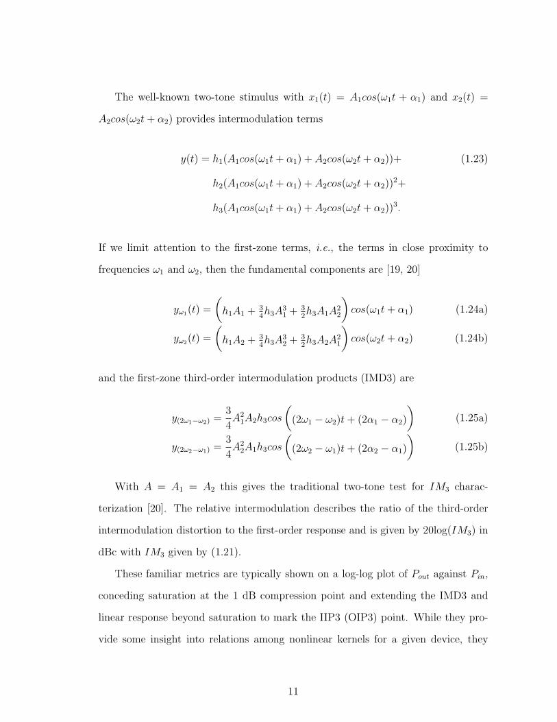
The well-known two-tone stimulus with x1(t) = A1cos(ω1t + α1) and x2(t) =
A2cos(ω2t+ α2) provides intermodulation terms
y(t) = h1(A1cos(ω1t+ α1) + A2cos(ω2t+ α2))+ (1.23)
h2(A1cos(ω1t+ α1) + A2cos(ω2t+ α2))2+
h3(A1cos(ω1t+ α1) + A2cos(ω2t+ α2))3.
If we limit attention to the first-zone terms, i.e., the terms in close proximity to
frequencies ω1 and ω2, then the fundamental components are [19, 20]
yω1(t) =
(h1A1 +
34h3A
31 +
32h3A1A
22
)cos(ω1t+ α1) (1.24a)
yω2(t) =
(h1A2 +
34h3A
32 +
32h3A2A
21
)cos(ω2t+ α2) (1.24b)
and the first-zone third-order intermodulation products (IMD3) are
y(2ω1−ω2) =3
4A2
1A2h3cos
((2ω1 − ω2)t+ (2α1 − α2)
)(1.25a)
y(2ω2−ω1) =3
4A2
2A1h3cos
((2ω2 − ω1)t+ (2α2 − α1)
)(1.25b)
With A = A1 = A2 this gives the traditional two-tone test for IM3 charac-
terization [20]. The relative intermodulation describes the ratio of the third-order
intermodulation distortion to the first-order response and is given by 20log(IM3) in
dBc with IM3 given by (1.21).
These familiar metrics are typically shown on a log-log plot of Pout against Pin,
conceding saturation at the 1 dB compression point and extending the IMD3 and
linear response beyond saturation to mark the IIP3 (OIP3) point. While they pro-
vide some insight into relations among nonlinear kernels for a given device, they
11

remain subject to the operating conditions at measurement and the assertion of
static (memoryless) low-order nonlinearity. In many cases, especially in modern
broadband communication systems, these simple measurements do not capture the
full range of nonlinear device behavior.
1.3 Measuring Volterra kernels
With this context there remains the question of how to measure the Volterra kernels,
which will provide a more accurate and rich characterization of the device. The
nonlinear system identification problem has very general application, and different
contexts place different demands on the measurement approach.
The field arguably started with nonlinear circuit analysis in 1942 when Norbert
Wiener evaluated a diode’s response to white noise [21, 22]. In many respects,
however, nonlinear identification has developed further in the context of biology and
control systems than in microwave and RF system analysis and design [23, 24]. For
microwave and RF systems and devices, nonlinear identification plays a role in both
circuit and device optimization [6, 19, 25–30] and linearization—e.g., mitigating the
consequences of unwanted nonlinearity [15].
Wiener recognized that stimulating a nonlinearity with white noise would excite
the full range of the nonlinear response [21, 31]. Lee and Schetzen refined this insight
to provide a correlation-based methodology that identified orthogonal mixtures of
Volterra kernels hn, called G-functionals Gn, with y(t) =∞∑n=0
Gn
[hn, x(t)
], using
stimuli x(t) that could be represented on a basis of orthogonal polynomials [7, 32, 33].
In this approach the orthogonal polynomials—Legendre, Laguerre, Hermite, Bessel—
were originally taken from special-case solutions (for particular boundary conditions)
of the Sturm-Liousville problem [7, 17, 34]. This measurement framework found
widespread application in fields ranging from nuclear science [35], to control systems,
fluid dynamics, and neuroscience [8, 17, 23, 36–39], and fostered extensive research
12
on stimulus signal design [8, 40–46].
Despite its application in other fields, and its origins in nonlinear circuit analysis,
Lee and Schetzen’s measurement framework did not find widespread application in
microwave and RF systems. For several years there was little effort to measure
Volterra kernels in nonlinear circuits [47]. The 1980’s saw renewed interest in using
multisine stimuli to measure low order Volterra frequency kernels [47].
Since the mid-1990’s the convergence of cheap digital processing power, the ad-
vent of complex modulation schemes that maximize spectral utilization, the prolifer-
ation of wireless communication devices, the push for wider bandwidth communica-
tion systems, and the demand for greater dynamic range and higher transmit power,
has placed increasing interest on nonlinear identification in communication systems
for both circuit optimization and, in particular, linearization. This work focuses
on measurement of a nonlinear transfer function, not the linearizing predistortion
resulting from inverting a measured nonlinear transfer.
From the specific context provided by a microwave transmitter system with a
power amplifier biased in nonlinear operation, we develop an approach of general
applicability suitable for measuring Volterra kernels in weakly nonlinear systems or
devices in any RF or microwave system.
1.4 Nonlinearity is the price of power amplifier efficiency
The power amplifier (PA) in modern communication systems is more efficient (it con-
sumes less DC power) in nonlinear operation [48].2 As a result, modern communica-
tion systems maximize efficiency by operating power amplifiers in compression, rather
than a linear regime. The loss in power added efficiency (PAE)(ηPAE = Pout−Pin
Pdc
)2“[N]o electronic device can maintain constant gain, and thereby linearity, if it depends on a limitedpower supply. Therefore, to be more power efficient, the system needs to draw less power from thesupply for the same amount of output power. This inevitably leads to higher gain compression,which, in turn, makes the system less spectrum efficient. This is the basis of the linearity-efficiencycompromise, also known as the power-spectrum efficiency trade-off.” ([48] at 44.)
13

from backing off to a linear regime can be dramatic, particularly with higher-order
modulation schemes [48–51]. Complex, spectrally-efficient modulation schemes like
ODFM or standards like CDMA can have peak to average power ratios (PAPR) on
the order of 10-12 dB [11, 51, 52]. High PAPR increases the PAE cost from backoff
to a linear operating point at peak signal amplitudes, creating pressure for increased
device linearity and dynamic range [53, 54].
The improved power added efficiency from nonlinear operation comes at a cost
of spectral regrowth and in-band distortion. Compliance with strict spectral mask
regulations and waveform quality metrics often requires linearization strategies like
digital predistortion. Digital predistortion, in turn, is often based on representing
the amplifier nonlinearity with a truncated Volterra series [5, 15, 55–58].
1.5 Memory effects in wideband microwave systems
The Volterra series can represent memory effects in a wide class of nonlineari-
ties including weakly nonlinear power amplifiers in transmit architectures. Short-
term memory involves high-frequency, passband effects with short time constants
on the order of ns, traceable to high-frequency component cutoffs and group delay
in impedance matching networks and filters [59]. Long-term memory involves low-
frequency effects with time constants on the order of µs, traceable to device biasing
networks, AGC loops, or semiconductor device heating and trapping (e.g., thermal
effects) [59]. In a two-tone test long-term memory can manifest as variation in IMD3
with tonal frequency separation [59], or asymmetric sidebands [60].
Regarding the Volterra series as a multidimensional convolution gives intuitive
sense of how it accounts for memory effects for modeling wideband communication
system power amplifiers. As suggested above, viewing the Volterra series as a multi-
dimensional Taylor series expansion of the nonlinear functional around a particular
operating point has a subtle but significant implication for measurement and behav-
14

ioral modeling.
While the Volterra series can exactly represent a given nonlinearity around a
particular operating point, for a given parameterization the model accuracy suffers
as the nonlinear operating point varies. The nonlinear system identified by measur-
ing coefficients at a given operating point (device electrical and thermal bias, load,
and signal stimulus), in other words, becomes less representative of actual system
nonlinearity as operating set point parameters vary increasingly from the conditions
at measurement. In practice this is addressed, in part, with lookup tables of coeffi-
cients associated with different operating conditions (temperature) when the model
is operationalized for predistortion [61]. The Volterra series models, in other words,
are highly particular, and do not generalize well to new operating conditions or de-
vices [15].3 This motivates approaches that can measure device nonlinearity during
system operation and subject to perturbations in nonlinearity determinants.
1.6 Limitations in existing nonlinear measurement
Accurately measuring nonlinear coefficients for a microwave or millimeterwave sys-
tem is notoriously difficult [47, 56, 57]. Within the microwave community, mea-
surement techniques have struggled to keep pace with advances in the sophisticated
behavioral modeling literature [15, 61].
3“[Behavioral model] accuracy is highly sensitive to the adopted model structure and the param-eter extraction procedure. Thus, it is of no surprise that distinct model topologies and differentobservation data sets may lead to a large disparity of model applicability and simulation results.In fact, if such a behavioral modeling approach may guarantee the accurate reproduction of thedata set used for its extraction or, eventually, of some other set pertaining to the same excitationclass, it is no longer obvious if it will also produce useful results for a different data set, a differentPA of the same family, or a PA based on a completely different technology. That is, contrary toan analytical model, a behavioral model tends to suffer from doubtful generality and predictivecapabilities.” ([15] at 1150.)
15

1.6.1 AM/AM, AM/PM models
Memoryless nonlinearities are frequently represented with AM/AM, AM/PM models
[3, 10, 14, 62–64]. Part of the appeal undoubtedly lies in the fact that the nonlinear
parameters can be measured on a network analyzer with a continuous wave (CW)
stimulus power sweep [62, 65]. These models specify ‘static’ nonlinear distortion
in amplitude (AM/AM) and phase (AM/PM) in response to the stimulus signal
amplitude. For a harmonic stimulus x(t) = A(t)cos(ωt + ϕ(t)) we represent the
output as
y(t) = G[A(t)]cos(ωt+ ϕ(t) + Ψ[A(t)]) (1.26)
with G[A(t)] representing nonlinear AM/AM distortion, and Ψ[A(t)] representing
the nonlinear AM/PM phase distortion [62]. The model can be used to predict
spectral regrowth and the adjacent channel power ratio (ACPR) for the measured
nonlinearity [62], and a physical basis for the observed behavioral model can be de-
scribed at different levels of generality in terms of device fundamentals [66] or circuit
theory [65]. The AM/AM, AM/PM representation can be expressed in terms of a
quasi-memoryless simplification of a truncated Volterra series, with complex lowpass-
equivalent coefficients [3, 11]. For convenience, the derivation in [3] is reproduced in
Appendix B.
The AM/AM, AM/PM models work for narrowband systems, but fail when de-
scribing RF power amplifier responses to wideband input signals and in increasingly
wideband systems like WCDMA and OFDM with carrier aggregation [3, 10, 64, 67].
A four-carrier WCDMA signal can have bandwidths of 20 MHz at a ∼ 2 GHz carrier
[10]. Accurately representing a nonlinearity in wideband systems requires modeling
long-term memory effects [3, 11, 62].
16

1.6.2 Measuring nonlinearities with a nonlinear vector net-
work analyzer (NVNA)
State-of-the-art measurement employs nonlinear vector network analyzers with peri-
odic or multisine stimulation and load-pull analysis, which can provide robust results
for design optimizations [28–30, 68, 69]. This static characterization, however, mea-
sures nonlinear response subject to potentially unrepresentative signals and relies on
bulky, expensive equipment unsuited to mobile communication form factors. Sinu-
soidal probes may elicit different nonlinear responses than representative signals with
complex modulation schemes encountered during device operation [1, 47, 70–74]. As
a result, it is desirable to consider a methodology that accurately measures nonlinear
responses to actual system waveforms, subject to varying in situ electric and thermal
bias, load, and memory effects, in a form compatible with mobile communications.
1.6.3 Reducing nonlinearities by predistorting the input with
the nonlinear transfer function inverse
Operational digital predistortion methods use inverse or adaptive regression methods
for parameter extraction, relying on the fact that the response is linear in its Volterra
series parameters [15, 17, 56–58, 75, 76]. While this has the advantage of estimating
Volterra kernels in response to actual signal excitations, these methods are limited
by the fact that the Volterra coefficients are generally not orthogonal [1, 7, 17, 31,
32, 36, 38, 77, 78]. This collinearity can result in high conditioning numbers [77, 78],
slowing adaptive estimation convergence [56] and biasing the nonlinear model by the
identification stimulus [78]. The collinearity can also result in wide estimation error
bounds, which are not necessarily reduced by increasing the number of samples [79].
17

1.7 A new spread-spectrum measurement approach
Given these limitations there is need for a methodology that accurately measures
nonlinearity stimulated by representative test signals, bias, and device load, while
avoiding a need to invert poorly conditioned matrices from a stimulus and response
analysis. It is desirable to provide a system that can track variations in the non-
linearity with changing stimuli or environment, while remaining compatible with
mobile communication form factors.
As with other nonlinear measurement frameworks [7, 28, 32, 35, 47], we treat
measuring Volterra kernels as conceptually distinct from identifying, for predistor-
tion, the nonlinear transfer inverse. For many predistortion analyses this may be a
distinction more honored in the breach than the observance, since these approaches
often leave the nonlinear measurement merely an implicit consequence of finding the
nonlinear transfer inverse. The distinction is nonetheless valuable, even if subse-
quent predistortion still entails the computational expense of inverting the measured
response, because it forces us to consider ways to address the conditioning problem.
1.7.1 Early spread-spectrum identification methods
Direct sequence spread-spectrum methods provide powerful tools that address these
measurement challenges. Prior efforts to identify nonlinear kernels using spread-
spectrum coding relied on single-carrier test signals compiled from forward link
CDMA input [80–83]. More particularly, [80, 81] probed a quasi-memoryless non-
linear response for a base station transmit power amplifier in DS-CDMA based a
single test signal formed by the product (XOR) of three duobinary PN sequences
from sequences already present in a baseband IS-95 forward link input signal. This
approach did not consider test signal design, or sampling the nonlinear coefficients
at different locations in multiple frequency space. Partly as a result, this approach
18

did not consider correlated noise on the kernel measurement that can arise from poor
selection of test signal sequences.
[82] investigated digitally correcting harmonic nonlinear distortion in pipelined
analog-to-digital converters (ADCs). This approach treated the distortion as a mem-
oryless, weakly nonlinear function of input voltage [82]. Like [80, 81], [82] developed
a test signal as a simple sum of duobinary, BPSK PN sequences. Unlike [80, 81],
however, [82] did not develop a test signal from existing signal components. Instead,
it specifically injected m duobinary, BPSK PN sequences to the ADC in order to
probe an mth-order nonlinear distortion, using correlation against suitable sequence
products (XOR) to estimate nonlinear coefficients. [82] recognized some correlated
noise from higher-order distortion on lower-order coefficient estimates, and proposed
algorithms to correct this effect. Like [80, 81], however, [82] only estimated a small
number of distortion coefficients in what we would call a single channel. This low-
dimensionality did not confront correlated noise that could result from improvident
choice of PN sequences in the test signal.
[83] built on [81] to consider, with basic simulations, how nonlinear distortion
corrupts CDMA coding, and suggested that known intermodulation codes could be
used to identify channel nonlinearity. However, [83] did not investigate test signal
generation or sources or remedies of correlated code noise in nonlinear identification.
These early approaches, in short, recognized the basic premises that spread-
spectrum tools provide a mechanism to measure nonlinearity in the background
during system operation; that this facilitates time-domain, correlation-based mea-
surement; and that systematic code intermodulation can (subject to some system-
atic higher-order correlated noise) uniquely identify a particular test nonlinearity.
These efforts, however, were limited to single channel, memoryless nonlinear mea-
surements that disregarded the rich frequency parameterization available through
this approach; gave little attention to test signal design; and did not consider the
19

relation between multi-channel test signals and correlated noise introduced by inter-
modulation.
1.7.2 A new spread-spectrum approach.
In this work we elaborate on a background time-domain approach using direct se-
quence spread-spectrum techniques that are compatible with any existing commu-
nication standard [84]. Unlike [80–82], this approach investigates test signal gener-
ation from first principles as a code domain design problem subject to systematic
intermodulation distortion constraints. Unlike [80, 81], the test signals are injected
during system operation, and the relation between test signal and operating signal
power is closely considered. Particular attention is given to correlated noise from
code domain intermodulation, particularly for rich frequency parameterization using
a multichannel test signal.
The spread-spectrum approach relies on nonlinearities in the device under test
(DUT) stimulated by actual operating signals, under actual electrical and thermal
bias and subject to in situ load matching. The spread pilots that facilitate mea-
surement are, by design, only small perturbations to the nonlinearity stimulated
by the desired operating signal. The proposed method injects spread pilots at de-
sired frequencies in the input signal path, and identifies the lowpass equivalent non-
linear parameters for a truncated Volterra series by correlating the DUT output
with intermodulation codes systematically generated by DUT distortion—at known
frequencies—for a given order nonlinearity.
The demonstration uses off-the-shelf components and a simple correlation-based
algorithm, suitable for acceleration and real-time parameter identification. The re-
sulting identification methodology provides a rich set of nonlinear parameter mea-
surements on a test device during its normal operation, with a nonlinearity stim-
ulated by actual operating signals, subject to actual electric and thermal bias and
20

Table 1.1: Spread-spectrum nonlinear measurement.
Multisine[28–30, 68, 69]
Regression /adaptation[56, 57, 67]
Spreadspectrum(this work)
Form bulky, expensive SoC / FPGA SoC / FPGA ∗
Representativestimulus
no yes yes
Directmeasure
yes no yes
Background no yes yes
Rich freq.parameterization
yes no yes
Computes inverseadaptation
no yes no
Memory kernels some variants [85, 86] at fs at Rc
Limits onestimate precision
interpolate / LUTunrepresentative stim
conditioning,convergence
arbitrary(process gain)
Suitable forreal-time measure
no yes yes
load conditions.
Table 1.1 highlights the spread-spectrum measurement approach developed here
in comparison to the limitations in the existing multisine (NVNA) and regression
approaches. Because each correlation provides a new parameter measurement, this
approach can track changes in the nonlinearity parameterization on intervals longer
than one dwell. The measurement proceeds without needing to invert poorly condi-
tioned matrices from regression on stimulus and response samples, and with precision
limited by the spread pilot code length (process gain).
Like a multisine analysis, the approach samples the nonlinear transfer at several
points in multidimensional frequency space dictated by the pilot frequency multiplex-
ing in a baseband test signal. But unlike a multisine analysis, the spread-spectrum
method identifies distinct in-band distortion terms without needing to isolate the dis-
tortion response in frequency. With proper pilot design, this approach can extract a
21

complete set of Volterra kernels over a given frequency range.
Although we show a proof of concept using a benchtop testbed with offline sig-
nal processing, by design the spread-spectrum methods use standard correlation
DSP blocks and—like the operational predistortion methods—the spread-spectrum
approach is ripe for acceleration in a FPGA or SoC, and integration with digital
transmitter architectures.
1.7.3 Organization
The dissertation is organized as follows.
Chapter 2 describes the novel spread-spectrum measurement architecture and
methodology, and provides proof of concept results from a benchtop demonstration
on a PA chain operated in compression on a 10 MHz bandwidth signal at 1960
MHz. The test signals and signal processing are carried out offline using algorithms
implemented in Matlab.
Chapter 3 provides a deeper discussion of the algebraic coding and spread pilot
design used in this demonstration, including an investigation of correlated noise
arising from the spread pilot design. A methodology is developed to identify safe
spread pilot combinations given the code length, number of spread pilots, and the
particular distortion terms being identified, so as to avoid pseudorandom correlated
noise that we call a code collision.
Chapter 4 provides conclusions and identifies future directions.
This work is the subject of these manuscripts:
22

A.R. Wichman, L.E. Larson, “Background Measurement ofRF System Nonlinearity Using Spread-Spectrum Methods,”2017 90th ARFTG Microwave Measurement Conference (ARFTG),2017 (in press).
A. R. Wichman and L. E. Larson, “A Background Spread-Spectrum Radio Frequency Nonlinear Identification Method-ology,” 2017 (in preparation).
A. R. Wichman and L. E. Larson, “Spread Pilot Design forCorrelation-Based Bandpass Nonlinear Identification,” 2017(in preparation).
23

CHAPTER Two
Spread-Spectrum Methods for Nonlinear Measurement
So, what can be said about the total [degree-3 nonlinear Volterra
system] steady-state response? Not much more than that it is a jungle
into which the prudent venture only with inkwell full.
—Wilson J. Rugh, Nonlinear System Theory:The Volterra/Wiener Approach (1981), p.214
This chapter reports a new correlation-based direct sequence spread-spectrum
technique that measures lowpass-equivalent Volterra coefficients for weakly nonlin-
ear RF systems. The methodology provides robust coefficient estimates at test sig-
nal amplitudes well below the operating signal level during normal system opera-
tion, demonstrating that the technique can be used for “background” nonlinearity
measurement. The methodology is demonstrated by measuring third-order Volterra
kernels for a PA chain operated in compression with a 10 MHz bandwidth signal at
1960 GHz.
The methods described below draw on results from the distinct fields of spread-
spectrum communications and nonlinear system identification theory. Good expla-
nations of spread-spectrum communications can be found in [87–91], while back-
ground on nonlinear identification and Volterra representations can be found in
[1, 7, 9, 15, 28, 31, 32], among other sources. See Appendix C (direct sequence
24

spread-spectrum), D (Volterra frequency interpretation).
2.1 Test System Architecture
We suppose a weakly nonlinear device is properly representated by a Volterra series
truncated to third-order. The third-order case often dominates the distortion for
RF power amplifiers (PAs) and should describe a wide range of weakly nonlinear
systems [3, 49, 70]. 1 For symmetric, triangular kernels a first-zone discrete lowpass-
equivalent third-order Volterra series has the form [10, 14]
y(n) =M−1∑m1=0
h1(m1)x(n−m1) + (2.1)
M−1∑m1=0
M−1∑m2=m1
M−1∑m3=m2
h3(m1,m2,m3)
× x(n−m1)x(n−m2)x(n−m3)∗.
The Volterra coefficient extraction is demonstrated with a coherent direct conver-
sion correlation receiver in a direct sequence spread-spectrum testbed [84]. Figure
2.1 shows the test signal generation. We generate sequences for spread pilots, to
probe the DUT nonlinear response, from a complex mixture a = a1 + ja2 of base-
band pseudoternary (PT) sequences a1,2 with an alphabet on [−2, 0, 2]. Each PT
sequence is formed from BPSK coded duobinary PN m-sequences as set forth in [92].
The underlying PN sequences have a primitive polynomial of degree r over GF(2),
code length N = 2r − 1, and form a pulse train at chip rate Rc.
At Rc, the complex pseudoternary (CPT) pilots ai(m) for channel i are pulse-
shaped with a raised-cosine filter having excess bandwidth α = 0.22, upsampled to
the desired DAC sample rate, and multiplexed to the baseband offset channel or
sub-band at ωi = 2πfi to form the spread pilot Aixi(n) with Ai the amplitude of the
1Extending the spread-spectrum approach to higher-order nonlinearities remains open for futurework.
25
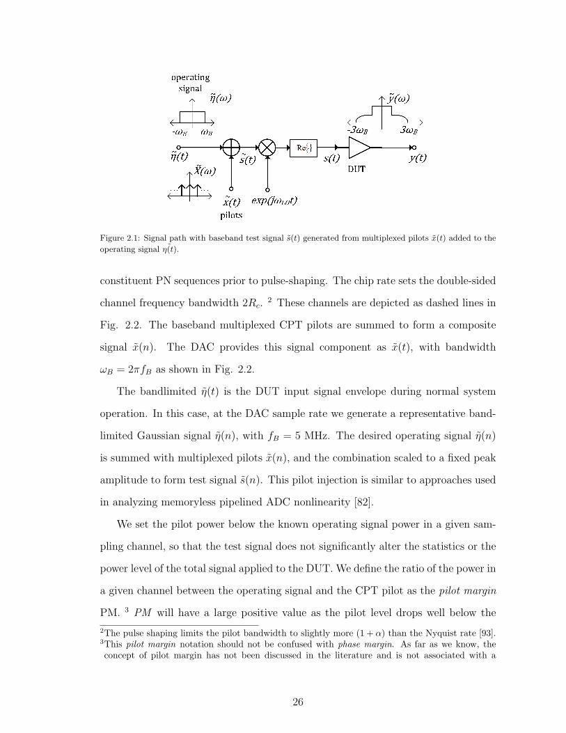
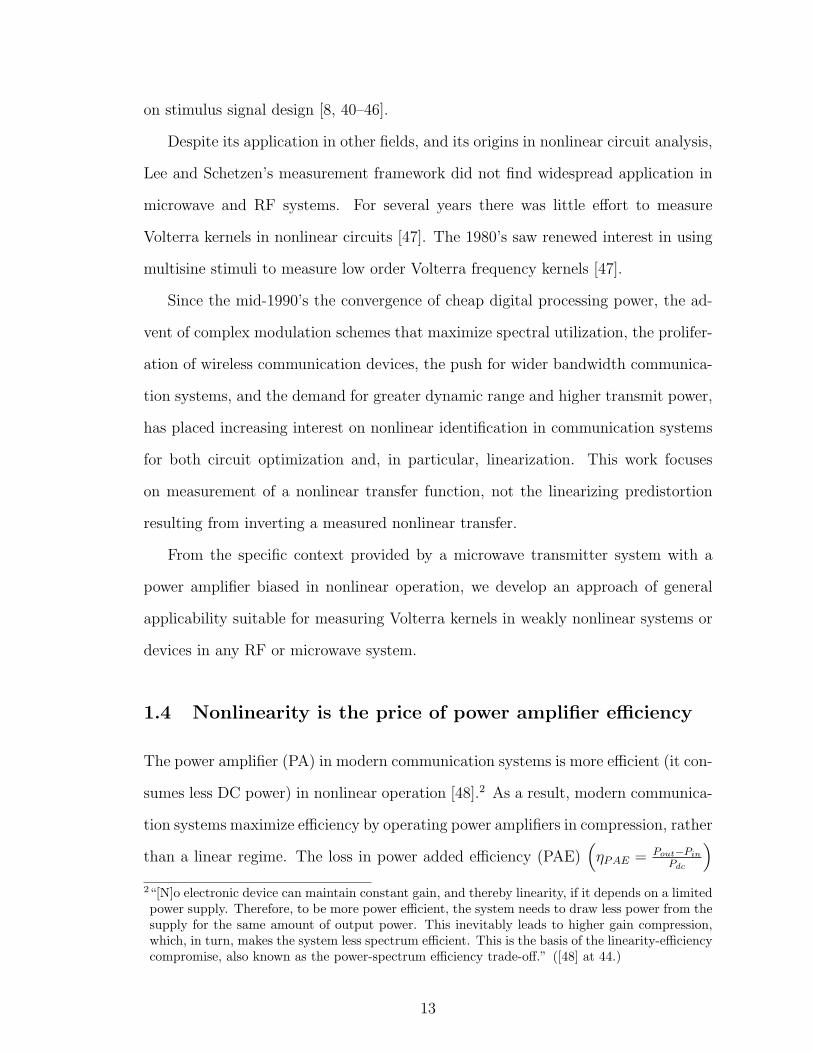
Figure 2.1: Signal path with baseband test signal s(t) generated from multiplexed pilots x(t) added to the
operating signal ˜η(t).
constituent PN sequences prior to pulse-shaping. The chip rate sets the double-sided
channel frequency bandwidth 2Rc.2 These channels are depicted as dashed lines in
Fig. 2.2. The baseband multiplexed CPT pilots are summed to form a composite
signal x(n). The DAC provides this signal component as x(t), with bandwidth
ωB = 2πfB as shown in Fig. 2.2.
The bandlimited η(t) is the DUT input signal envelope during normal system
operation. In this case, at the DAC sample rate we generate a representative band-
limited Gaussian signal η(n), with fB = 5 MHz. The desired operating signal η(n)
is summed with multiplexed pilots x(n), and the combination scaled to a fixed peak
amplitude to form test signal s(n). This pilot injection is similar to approaches used
in analyzing memoryless pipelined ADC nonlinearity [82].
We set the pilot power below the known operating signal power in a given sam-
pling channel, so that the test signal does not significantly alter the statistics or the
power level of the total signal applied to the DUT. We define the ratio of the power in
a given channel between the operating signal and the CPT pilot as the pilot margin
PM. 3 PM will have a large positive value as the pilot level drops well below the
2The pulse shaping limits the pilot bandwidth to slightly more (1 + α) than the Nyquist rate [93].3This pilot margin notation should not be confused with phase margin. As far as we know, theconcept of pilot margin has not been discussed in the literature and is not associated with a
26

Figure 2.2: Spectrum of baseband test signal pilots X(ω) arrayed in multiple channels spanning the oper-ating signal η(ω).
operating signal level. The resulting intermodulation distortion products in a given
channel will have inherently negative signal-to-interference-and-noise ratios (SINR),
where the signal in this case is the intermodulated spread pilots and the noise is
the (amplified) operating signal. Clearly these low SINR conditions require high
processing gain PG = 10log10(N) dB. We can set PG by increasing the m-sequence
order r, and thus increasing the code length N and the associated code interval or
dwell D = N · Tc at Tc = 1/Rc. 4
As shown in Fig. 2.3, a two-channel 16-bit DAC supplies the test signal s(t) to
an IQ modulator, which applies the passband test signal to an HP8763A transfer
switch. The linear path is used for “through” calibration. The transfer switch output
is demodulated by direct conversion and the distorted I, Q envelope is digitized with
a two-channel 16 bit ADC. Each I and Q channel on the DAC and ADC has its own
generally accepted notation.4While our initial goal was to demonstrate kernel extraction with the pilot signal power 20 dBbelow the operating signal in a given channel (20 dB PM), as discussed in the text with 60 dBprocess gain we ultimately demonstrated consistent and repeatable kernel measurements to slightlyunder 12 dB pilot margin. Measuring under the 20 dB PM may require longer signals and higherprocessing gain, which may push the technical limits of the demonstration testbed components.
27
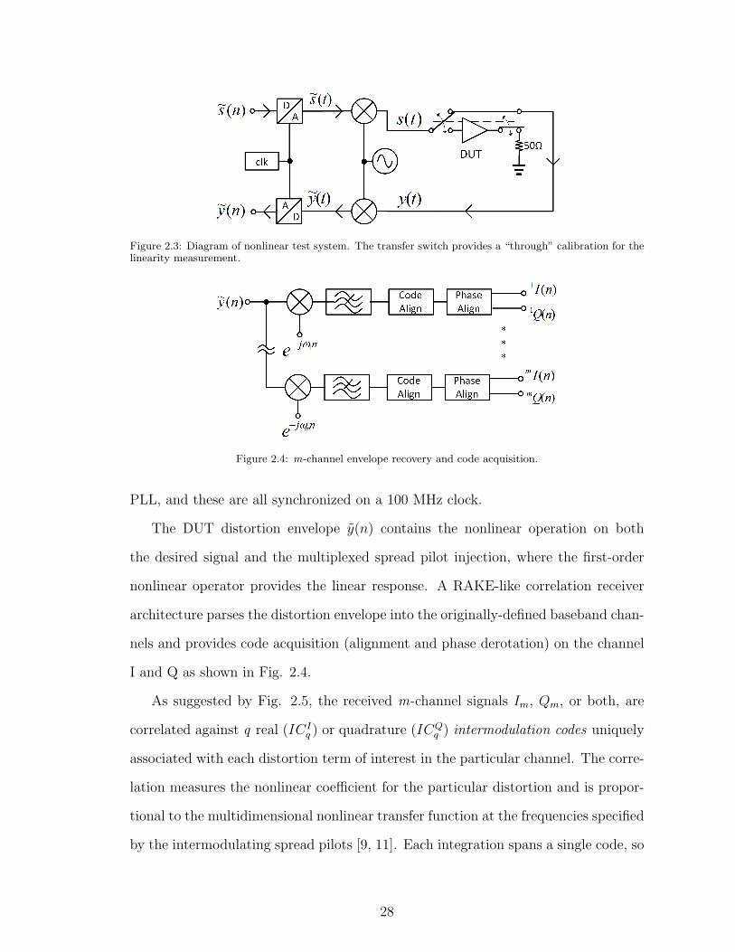
Figure 2.3: Diagram of nonlinear test system. The transfer switch provides a “through” calibration for thelinearity measurement.
Figure 2.4: m-channel envelope recovery and code acquisition.
PLL, and these are all synchronized on a 100 MHz clock.
The DUT distortion envelope y(n) contains the nonlinear operation on both
the desired signal and the multiplexed spread pilot injection, where the first-order
nonlinear operator provides the linear response. A RAKE-like correlation receiver
architecture parses the distortion envelope into the originally-defined baseband chan-
nels and provides code acquisition (alignment and phase derotation) on the channel
I and Q as shown in Fig. 2.4.
As suggested by Fig. 2.5, the received m-channel signals Im, Qm, or both, are
correlated against q real (ICIq ) or quadrature (IC
Qq ) intermodulation codes uniquely
associated with each distortion term of interest in the particular channel. The corre-
lation measures the nonlinear coefficient for the particular distortion and is propor-
tional to the multidimensional nonlinear transfer function at the frequencies specified
by the intermodulating spread pilots [9, 11]. Each integration spans a single code, so
28

Figure 2.5: Correlations on m channel received signal Im or Qm, against unique real (ICIq ) or quadrature
(ICQq ) intermodulation codes, measure the particular q nonlinear distortion coefficient associated with the
distortion in that channel. Each correlation separates a unique distortion term.
that this measurement applies to nonlinearities that are slowly varying on the order
of one dwell. Put differently, this approach can measure temporal variations in the
nonlinear response at a resolution of N · Tc. This resolution is therefore decreasing
(e.g., the dwell is increasing) in code length (process gain), but increasing in chip
rate Rc.
2.2 Code design for correlation on intermodulation
In order to explain the coefficient measurement at the correlation receiver we de-
scribe the spread pilot design, the nonlinear distortion, and the spreading sequence
intermodulation in greater detail below.
The intermodulated spread pilot coding leads to an unexpected source of corre-
lated noise. We refer to this as “pseudorandom correlated code noise,” because the
origins and incidence are related to a “pseudorandom” interplay among the phases of
the underlying pseudorandom sequence. 5 All else being equal, unless corrected, this
unexpected and unwanted correlated noise can result in a systematic bias leading to
inaccurate distortion kernel estimates. Chapter 3 provides a more extensive treat-
ment addressing code design considerations to avoid correlated noise. In order to
describe the spread-spectrum measurement, however, the following discussion simply
5In one form that we call a “code collision,” this correlated noise resembles the degeneracy calleda “hash collision” in computer science. See Chapter 3.
29

assumes that correlated noise has been addressed as set forth in Chapter 3.
2.2.1 Spread pilot design
The complex pseudoternary (CPT) pilot sequence a = a1 + ja2 is formed from PT
sequences
a1 = c1 − c2 (2.2)
a2 = c3 − c4
where each constituent m-sequence cq, q ∈ [1, 4] is drawn from a reference duobinary
BPSK sequence c at a specified initial condition (register state). There are, in other
words, four PN sequences per CPT sequence (or CPT pilot). These defines a nine-
point ternary constellation as shown in Fig. 2.6a with an alphabet on [−2, 0, 2].
The periodic reference m-sequence c provides N cyclically-shifted orthogonal PN
sequences, each with a different phase p ∈ [0, N − 1] [88]. In particular, we write the
PT sequence in channel i
aqi = T pq,i(c− T 1c) (2.3)
where T is the cyclical left shift operator; pq,i and pq,i + 1 are the PN phase or
chip offsets defining the underlying PN sequences for aqi ; and q identifies the real
(1) or imaginary (2) PT sequence in ai following (2.2). With M channels there are
4M PN sequences in the composite test signal, and (2.3) constrains the sequence
specification to 2M phase choices p relative to the reference sequence c. These code
phases are specified, given the number of CPT pilots and code length, so as to impose
orthogonality on the intermodulation codes for the coefficient measurement.
Substituting (2.3) in (2.2) provides a way to describe each CPT pilot sequence
30

(a)
(b)
Figure 2.6: CPT detail. (a) CPT constellation, (b) Normalized pseudoternary (PT) autocorrelation⟨a1,a1
⟩
ai in channel i in terms of its constituent PN sequences cqi with q ∈ [1, 4]. The
intermodulation codes used in the distortion measurements are orthogonal XOR
combinations of the constituent BPSK coded PN sequences in each CPT sequence.
The coefficient measurement correlates the received channel signal components I orQ
against intermodulation codes expressed in terms of these underlying PN sequences.
31

The periodic autocorrelation for any BPSK coded duobinary m-sequence u is
θu,u(i) =⟨u, T iu
⟩(2.4)
=N−1∑n=0
u(n)u∗(n+ i) =
N, i mod N = 0,
−1, else
using the property that the product of BPSK-encoded bits is the XOR or modulo 2
addition of those bits [88]. In other words, as noted above, each cyclically-shifted m-
sequence is orthogonal to every other cyclically-shifted m-sequence, so that a given
binary polynomial order r defines N orthogonal m-sequences [87, 88]. 6
The PT sequence autocorrelation is somewhat different from the underlying PN
sequences. It has a normalized autocorrelation as shown in Fig. 2.6b, and is identi-
cally zero for N − 3 chips.
For the nonlinear measurement, we are interested in correlating the complex mix-
ture of the pseudoternary pilots, as intermodulated by the nonlinear DUT, against
selected PN sequences representing intermodulation codes. By way of example, us-
ing the well-known PN correlation properties [88], we observe for a single CPT pilot
and underlying PN sequence,
⟨ai, c
1i
⟩= (N − (−1)) + j0 (2.5)
= N + 1,
6Note that the finite nonzero cross correlation result (-1) means that the ‘orthogonality’ providedby the PN sequence autocorrelation is only an approximation. If we normalize the autocorrelationby dividing out peak cross correlation N , we can drive the normalized PN sequence autocorrelationarbitrarily close to zero as we increase the coding process gain (code length N). The consequence of
this divergence from the traditional mathematical description of orthogonality(e.g., ⟨a,b⟩
|⟨a,a⟩| = δab
)is nonzero spread code noise.
32

while for a CPT pilot with PN sequence from a different CPT pilot,
⟨ai, c
1j
⟩= 0, i = j. (2.6)
This cross correlation will be the foundation for the correlation-based measurement
of the DUT nonlinearity.
2.2.2 Nonlinear distortion
Before we can identify the intermodulation codes associated with each nonlinear
distortion term, we need to consider how the nonlinearity operates on particular
spreading codes. While this information could be gleaned from a truncated Volterra
series in frequency domain with bandlimited spread pilots, the time-domain pro-
vides a more informative perspective consistent with how the spreading sequences
and correlation receivers are implemented. Appendix E provides a more extensive
development of the generalized multitone analysis summarized below.
By reference to Fig. 2.3 the first-zone DUT passband output is y(t) = (F
G)[s(t)], where G is a nonlinear operator, F is a first-zone filter, H = (F G) is the
first-zone nonlinearity being measured, and s(t) is the composite signal applied at
the DUT. Suppose for discussion we disregard the desired signal and only consider
intermodulation on pilots, so that s(t) = x(t),
x(t) =∑i
xi(t) (2.7)
and
xi(t) = Re
Ψi(t)
, (2.8)
33

Ψi(t) = Aixi(t)exp(jωit)exp(jωLOt) (2.9)
with Aixi(t) the baseband spread pilot corresponding to the pulse-shaped CPT se-
quence ai with PN sequence amplitude Ai, and Aixi(t)exp(jωit) the multiplexed
CPT pilot for channel i. In terms of the analytic signal Ψ(t) =∑
i Ψi(t), and the
first-zone cubic distortion terms have the form Ψ(t)Ψ(t)Ψ(t)∗ where ∗ is complex
conjugation.
With three spread pilots at (i, j, k) ∈ [1, 2, 3], Ψ(t) = Ψi(t) + Ψj(t) + Ψk(t). If
we first limit our attention to a memoryless cubic distortion, then operating on the
three pilots a cubic distortion generates eighteen difference frequency products in the
first zone, each having the form Ψi(t)Ψj(t)Ψ∗k(t), and each at an offset (baseband)
frequency i + j − k, using the indices as a shorthand for the applicable CPT pilot
offset frequencies.
At this point we define a cubic distortion taxonomy in terms of the pilots that con-
tribute to a distortion term. The cubic nonlinearity generates four distinct distortion
types that we call self-modulation (SMD3), cross-modulation (XMD3), intermodu-
lation (IMD3), and triple product (TPD3) distortions, falling at f , with phase ϕ,
scaled by amplitude A, according to the rules shown in Table 2.1.7
Taking a single pilot Ψi(t), for example, the resulting cubic distortion term is
Ψi(t) (Ψi(t)Ψ∗i (t)) at i ; with two pilots Ψi(t) and Ψj(t), i = j, cross-modulation
distortions are Ψi(t)(Ψj(t)Ψ
∗j(t))at i and Ψj(t) (Ψi(t)Ψ
∗i (t)) at j ; the familiar in-
7We use this taxonomy to name particular first-zone third-order distortion permutations using therules in Table 2.1. For the most part this convention is more specific than general usage. TheIMD3 terminology has fairly well-understood usage in RF, although this terminology is sometimesapplied indiscriminately to refer to all in-band third-order distortions [19, 20]. Third-order cross-modulation XMD3 has a more general usage describing the transfer of AM modulation from a highpower blocker to a signal of interest, although in this context we use XMD3 to describe distortionfrom equal amplitude and bandwidth pilots [19, 20]. As used in this distortion taxonomy, XMD3is sometimes called third-order desensitization [19]. In the sense used here, SMD3 is also calledthird-order compression or expansion [19]. As far as we know, there is no generally acceptedterminology to describe the TPD3 distortion terms–and few published discussions separately seemto consider these particular distortions. Their presence, however, requires attention and is readilyapparent when considering the first-zone distortion permutations. See Table 2.1, Appendix E.
34

termodulation distortion terms are Ψi(t)Ψi(t)Ψ∗j(t) at 2i − j and Ψj(t)Ψj(t)Ψ
∗i (t)
at 2j − i; and so on. Two pilots engender SMD3, XMD3, and IMD3; three pilots
are needed to provide TPD3. IMD3 and TPD3 can contribute to spectral broaden-
ing, while SMD3 and XMD3 always fall on top of an underlying pilot as “in-band”
distortion.
In a discretized lowpass-equivalent formulation, the memoryless cubic envelope
distortion term for spread pilots at ijk is
yijk3 (n) =
(34α1
)AiAjAkh
ijk3 xi(n)xj(n)x
∗k(n) (2.10)
where the ijk superscript gives the cubic distortion provenance.8 The scalar α1 comes
from the multinomial (cubic) expansion (Ψ(t) + Ψ∗(t))3 on the real passband signal,
and is (1, 2, 1, 2) for distortions (SMD3, XMD3, IMD3, TPD3). These nonlinear
coefficients hijk3 are thus similar to those identified in a multisine analysis, which
can be viewed as sampling the multidimensional nonlinear transfer at discrete points
in multidimensional frequency space [6]. The spread pilots, by comparison, can be
regarded as sampling the multidimensional nonlinear transfer in discrete volumes in
multidimensional frequency space, with the volume dimensions set by the two-sided
channel bandwidth 2Rc. See generally Appendix D.
2.2.3 Intermodulation codes for memoryless cubic nonlin-
earity
Using this taxonomy, the cubic distortion intermodulates any three spread pilots ijk
as the XOR of the associated CPT sequences. With BPSK coded PN m-sequences,
the XOR is obtained as the bitwise product of the underlying sequences. Table
8We note in passing that the distortion envelope formulation in (2.10) is mathematically analogousto a nonlinear polarization vector with difference frequency generation from three-wave mixing innonlinear optics, where the Volterra coefficient is analogous to the susceptibility matrix element[94].
35

Table 2.1: Third-order distortion terms.
Type Rule f ϕ A
SMD3 i = j = k i ϕi A3i
XMD3i = j, j = ki = j, i = k
ij
ϕi
ϕj
A2jAi
A2iAj
IMD3 i = j, j = k 2i− k 2ϕi − ϕk A2iAk
TPD3i = j, i = k,
j = ki+ j−k
ϕi + ϕj
−ϕkAiAjAk
Table 2.2: CPT Intermodulation.
Type CPT Mixing
SMD3aiaia
∗i = 6(c1i − c2i )− 2(c134i − c234i )
+j[6(c3i − c4i )− 2(c123i − c124i )
]XMD3
aiaja∗j = 4(c1i − c2i )− 2(c12j + c34j )(c1i − c2i )
+j[4(c3i − c4i )− 2(c12j + c34j )(c3i − c4i )
]
IMD3
aiaia∗k =
2(c34i − c12i )(c1k − c2k)
+2(c1i − c2i )(c3i − c4i )(c
3k − c4k)
+j
−2(c34i − c12i )(c3k − c4k)
+2(c1i − c2i )(c3i − c4i )(c
1k − c2k)
TPD3aiaja
∗k =
(c1i − c2i )(c
1j − c2j)(c
1k − c2k) + . . .
+j+ . . .− (c1i − c1i )(c
1j − c1j)(c
3k − c4k)
2.2 reports the CPT intermodulation associated with each cubic distortion type,
expanding each CPT sequence in terms of its underlying PN sequences, using a
contracted notation cxyzi to note the PN sequence XOR with PN sequences all taken
from channel i, and observing that cqi (n) · cqi (n) = 1 ∀n ∈ [0, N − 1].
Given the intermodulation products, it remains to select a triple PN sequence
XOR, or pilot triplet, as an intermodulation code (IC) for each particular distortion
type at ijk. By inspection the choice of IC is not unique. Table 2.3 shows represen-
tative candidate IC for the real and quadrature components of each cubic distortion.
These IC are shown in the correlation on the corresponding CPT triplet, with the
36

Table 2.3: Intermodulation Codes.
Type Correlation Result
SMD3 ⟨aiaia∗i , c
234i ⟩ 2(N + 1)
⟨aiaia∗i , c
124i ⟩ j2(N + 1)
XMD3⟨aiaja
∗j , c
12j c2i
⟩2(N + 1)⟨
aiaja∗j , c
12j c4i
⟩j2(N + 1)
IMD3 ⟨aiaia∗k , c
34i c1k⟩ 2(N + 1)
⟨aiaia∗k , c
34i c4k⟩ j2(N + 1)
TPD3⟨aiaja
∗k , c
1i c
1jc
1k
⟩(N + 1)⟨
aiaja∗k , c
1i c
1jc
4k
⟩j(N + 1)
expected ideal correlation output. We rely on the shift-and-add property [88], ap-
plied twice in series, to ensure that the IC code triplet is itself an m-sequence in
c.
We require that the ICs used to measure each distortion are mutually orthogonal.
Since we measure distortion on a channelized basis, it is sufficient to require that
each IC used to measure a distortion is orthogonal to every other code product that
appears in the same channel as the distortion. In the remaining discussion we set the
2M PN sequence phases of code offsets in the CPT pilots to satisfy the requirements
of the shift-and-add property, as well as this orthogonality requirement—with one
caveat. By inspection Table 2.2 shows that the SMD3 and XMD3 distortions include
a scaled version of the original, underlying CPT pilot sequence, falling in the same
channel as the underlying CPT pilot. This represents coded correlated noise on the
linear response (the first-order Volterra coefficient) and can, if desired, be subtracted
from the linear response estimate once the associated cubic distortion envelope coef-
ficient is estimated. The remaining intermodulation terms in the SMD3 and XMD3,
however, remain orthogonal to the constituent PN sequences in the underlying CPT
pilot and provide candidate intermodulation codes.
37

2.2.4 Intermodulation codes for memory representations
The spread-spectrum measurement also extends to memory coefficient measurements
by a modified choice of IC. In this section we show the extension in terms of a
memory polynomial [67] and generalized memory polynomial [56],two behavioral
models commonly used to develop digital predistortion for weak PA nonlinearities.
2.2.4.1 Memory polynomial
We write a memory polynomial model with order K and memory depth M , in terms
of lowpass equivalent Volterra coefficients, limited to first-zone, as [67]
y(n) =
⌈K2⌉−1∑
k=0
M−1∑m=0
h(2k+1)mx(n−m)|x(n−m)|2k (2.11)
or for cubic distortion with K = 3
y(n) =M−1∑m=0
h1mx(n−m) (2.12)
+M−1∑m=0
h3mx(n−m)|x(n−m)|2.
The memory polynomial has the form of the SMD3 distortion discussed above.
For a given sampling channel we can identify coefficients h3m to arbitrary memory
M by choice of the intermodulation code. Instead of the SMD3 CPT sequence ex-
pansion aiaia∗i in Table 2.2, we select the corresponding IC from terms found on
expanding the suitably delayed CPT sequences T−maiT−maiT
−ma∗i in their under-
lying PN sequences (using a shorthand T−m = TN−m for delay in terms of a cyclical
left shift). In the memory polynomial, for example, the corresponding IC take the
form T−mc2iT−mc3iT
−mc4i and T−mc1iT−mc2iT
−mc4i .
38

The result is a memory polynomial representation for a given channel, with mem-
ory resolution at the chip interval Tc.
2.2.4.2 Generalized memory polynomial
The lowpass-equivalent generalized memory polynomial with orderK, memory depth
M , and cross-term G, limited to first-zone terms, has the form [56]
y(n) =
⌈K2⌉−1∑
k=0
M∑m=0
akmx(n−m)|x(n−m)|2k (2.13)
+
⌈K2⌉−1∑
k=0
M∑m=0
G∑g=1
bkmgx(n−m)|x(n−m− g)|2k
+
⌈K2⌉−1∑
k=0
M∑m=0
G∑g=1
ckmgx(n−m)|x(n−m+ g)|2k.
As with the memory polynomial formulation, given the memory depth m and cross-
term g Table 2.4 shows the form of CPT expansion in channel i to identify in-
termodulation codes for the SMD3-like third-order generalized memory polynomial
coefficients. As above, the memory resolution is provided at the chip interval Tc
rather than the sample rate fs.
Table 2.4: CPT expansion for Generalized Memory Polynomial intermodulation codes.
Coefficient CPT expansion
akm aiaia∗i ⇒ T−maiT
−maiT−ma∗
i
bkmg aiaia∗i ⇒ T−maiT
−(m+g)aiT−(m+g)a∗
i
ckmg aiaia∗i ⇒ T−maiT
−(m−g)aiT−(m−g)a∗
i
The memory and generalized memory polynomial representations operate on the
stimulus x(t) without regard for particular distortion components within the DUT
output. Because the spread-spectrum measurement distinguishes in-band distortion
terms on the basis of CPT pilots contributing to the distortion, this approach might
enable new memory predistortion models that leverage this frequency-selective dis-
39

Figure 2.7: Measured baseband response for linear and DUT signal paths at PM 9 dB.
tortion measurement.
2.3 Measurement Results
We demonstrate the technique by measuring frequency-dependent third-order Volterra
coefficents on a representative RF power amplifier. In this work, the DUT in Fig. 2.3
consists of a MiniCircuits ZX60-242LN-S+ in series with MiniCircuits UWB ZX60-
V62+ PA. We use five CPT pilots with chip rate Rc = 1 MHz centered at baseband
f=[−4,−2, 0, 2, 4] MHz, as shown in Fig. 2.2, with the CPT pilots formed from
duobinary m-sequences with primitive polynomial of order r = 20. This provides
code length N = 220 − 1 with process gain PG ∼ 60 dB and dwell D = 1.05 sec.
The full scale range for s(n) is ±800 mV at the I and Q inputs to the quadrature
modulator. This signal amplitude drives the DUT into compression. The ADC sam-
ples at fs = 125 MHz, much higher than twice the spectral broadening for the cubic
distortion envelope on the 5 MHz wide baseband test signal. We use fLO = 1960
MHz, within the operating spectrum for the DUT PA chain.
The channel pilot signal power is set for a range of PM cases from 0 to 21 dB
40

in steps of 3 dB. A reference case with no operating signal (pilots only) is also
included. The transfer switch toggles the DUT into the signal path after we capture
five dwells (complete codes) through the linear calibration path. Fig. 2.7 shows the
linear input and DUT output envelope power densities with PM 9 dB at a typical
operating point.
Within the baseband operating signal η(ω), the five pilots combine for 85 frequency-
dependent cubic distortion terms, each centered on one of the five original channels.
The cubic distortion terms include spectral broadening from IMD3 and TPD3, and
additional distortion channels can be defined within this spectrally broadened region.
To make this more explicit, Fig. 2.8 shows the measured envelope for intermod-
ulation distortion using five CPT pilots and no operating signal. Fig. 2.8a shows
the linear testbed response to a stimulus that arrays five CPT pilots at [-4, -2, 0,
2, 4] MHz, each at the center of 2 MHz sampling channels. Within each sampling
channel the CPT pilots have a blue noise-like spectra with a notch at DC, a conse-
quence of the CPT pilot autocorrelation having zero mean as shown in Fig. 2.6b.
For visualization purposes a small DC component was added to each CPT pilot prior
to forming the multiplexed composite shown in the Fig. 2.8a; in keeping with the
objective of minimizing the test signal perturbation on the device nonlinear set point
we refrain from marking channels with this DC component in the actual test signals
such as shown in Fig. 2.7. The DC is visible as a frequency impulse marking the
center of each CPT pilot spectrum and each associated sampling channel in the test
signal. The five CPT pilots / channels are labeled A to E.
Fig. 2.8b shows the first-zone distortion envelope in response to the stimulus
in Fig. 2.8a. The response in this example is in fact strongly nonlinear, which
helps emphasize the potential sampling channel identification options in the first-
zone spectral broadening. The “in-band” distortion terms are associated with the
original channels A-E, while the upper sideband spectral broadening is associated
41

(a)
(b)
Figure 2.8: Measured first-zone intermodulated distortion envelope for test signal comprising five CPTpilots spanning 10 MHz offset (5 MHz baseband) spectrum as shown for the operating signal of interestin Figs. 2.7 and 2.2. Fig. 2.8a shows the measured linear testbed response to a composite CPT-onlytest signal. A small DC component is added to each pilot. The DC component is visible as a frequencyimpulse at the center of each multiplexed CPT pilot and associated test signal sampling channel, labeledA to E. Fig. 2.8b shows the measured distortion envelope spectrum for the stimulus in Fig. 2.8a with pilotintermodulation including third-order (5 to 15 MHz) and fifth-order (5-25 MHz) spectral broadening withinthe first zone. The (intermodulated) DC components provide frequency impulses marking the center ofeach potential sampling channel in the resulting intermodulated distortion envelope, with the visible upperspectral broadening labeled F to O.
42

with channels F-O (channels for lower sideband spectral broadening are not labeled).
The third-order spectral broadening is visible in the envelope spectrum at 5-15 MHz
(channels F-J), and fifth-order spectral broadening is visible at 5-15 MHz (channels
F-J) as well as 15-25 MHz (channels K-O).
While we can recover distortion coefficient magnitudes for each particular IMD3
and TPD3 distortion term contributing to the spectral broadening in channels F-
J (and for this measurement spectrally-broadening fifth-order distortion terms in
channels F-O) in Fig. 2.8 (and the lower sideband counterparts), we do not have
a phase reference against which to evaluate the distortion coefficient phase in the
spectrally-broadened region.
Within the “in-band” channels (A-E), the underlying linear CPT pilot provides
a phase reference for evaluating the particular distortion term phase. We sample
the linear CPT pilot, as shown in Fig. 2.8a, during a ’calibration’ interval prior to
toggling the transfer switch and applying the test signal to the DUT. As a result,
for the demonstration and measured distortion in Fig. 2.7 we restrict our attention
to these “in-band” distortion terms so that we can use the associated linear pilots as
relative phase references to determine the phase estimates for the distortion kernels.
2.3.1 Correlation measurement results
2.3.1.1 Linear coefficients
For the first-order complex coefficient in channel i, correlating the received signal
envelope Ii (Qi) on PN sequences from the injected CPT pilot sequences c1i (c3i )
and using (2.5) yields a correlation output zi11,12 proportional to the memoryless
first-order lowpass-equivalent Volterra coefficient estimate ˆhi11 or ˆhi
12,
zi11,12 =ˆhi11,12(N + 1) · SF1 · Ai + SCN (2.14)
43

Figure 2.9: Measured complex linear transfer coefficient components for more than 50 dwells after codealignment on center channel with 1960 MHz LO. Shaded region marks calibration interval routing signalthrough linear path on testbed.
Table 2.5: Measured linear coefficients.
f ¯|H1|(a.u.) std ¯|H1| ∠H1 () std ∠H1
-4 16.63 0.0017 -98.70 0.0086
-2 16.81 0.0018 -103.80 0.0090
0 16.93 0.0018 -109.16 0.0095
2 17.02 0.0018 -114.55 0.0102
4 17.05 0.0017 -120.08 0.0108
with ˆhi1 =
ˆhi11+jˆhi
12. In this formulation Ai is the PN amplitude in the CPT pilot at
the DUT input. The second term in (2.14) is the spread code noise (SCN ) residual
from correlating the operating signal η(n) against a pulse train from the IC code, in
this case the PN sequence c1i (c3i ). For an uncorrelated operating signal and infinite
length code the SCN should tend to zero; with finite code lengths, however, the SCN
will be a small finite quantity compared to the first term in (2.14). The SCN sets a
noise floor that limits the Volterra coefficient extraction at low SINR values, which
can be a binding constraint for measuring higher-order nonlinear coefficients. We
limit the SCN by increasing the process gain PG (code length N).
Calibration scaling factor SF1 is determined from kernel measurement on signal
44

through the testbed linear path prior to switching in the DUT. Figure 2.9 shows the
measured 0 MHz baseband channel linear coefficient components for the signal and
DUT described above. Each marker is the measured real (ˆh11) or imaginary (ˆh12)
components of the first-order Volterra coefficient (e.g., the linear DUT response in
channel i) over one dwell. The shaded regions show a calibration interval, during
which the testbed routes the signal through a linear path. This persists until reading
5 dwells of signal from commencing the data capture, at which point we trigger the
transfer switch and apply the test signal to the DUT. 9 After a brief interval that
includes a mechanical switching transient and the DUT nonlinear operating point
adjusting to the newly applied test signal, the correlation output settles on stationary
magnitude estimates at each integration.
We specify a reference memoryless linear path impulse response as a unit transfer
with no rotation, or hi
1 = 1∠0. The linear kernel extraction is “self-calibrating” in
the sense that we de-embed the effect of linear testbed propagation by rotating and
scaling the ˆh1 =ˆhi11+
ˆhi12 measured during the calibration phase (prior to switching)
to match the reference linear response. The multiplier that accomplishes this rotation
and scaling is the calibration scaling factor SFi. The shaded regions on Fig. 2.9 show
the calibrated unitless linear response in I and Q prior to switching.
The change in the measured coefficients in Fig. 2.9 after switching shows the
effect of the DUT, e.g., it provides the measured linear coefficient components. Table
2.5 shows the mean magnitude and angle measurements for each channel, starting
9The choice of dwells for linear calibration is arbitrary, subject to providing at least one dwell pastcode acquisition. Since code acquisition requires up to one dwell, a single linear measurementrequires capturing at least 2 dwells of data. In this example, we selected 5 dwells as sufficient todampen any testbed measurement transients (and provide some confirmation for a linear steadystate response), while maximizing the remaining number of measurements on the DUT given afixed number of total dwells in the data capture. The results in Fig. 2.9 confirm this assumption;indeed, there is no transient visible on the linear response. Note that the system toggles thetransfer switch based on data capture from the run initiation, not the acquisition mark, but themechanical switch itself has a finite latency. In Fig. 2.9 this means that the system toggled theswitch before the fifth dwell (from alignment, as plotted), but by inspection the switching transientdoes not begin until after that fifth dwell (from alignment).
45

at two dwells past the switching mark. The PA chain provides ∼ 25 dB gain in each
channel, consistent with the amplifier specifications.
2.3.1.2 Cubic coefficients
The cubic distortion correlation is likewise proportional to the relevant Volterra ker-
nels, but includes additional scaling factors and presents different calibration chal-
lenges than the first-order coefficient correlations in (2.14).
Given a particular cubic distortion at i+j−k, we select a suitable intermodulation
code from the CPT pilot sequence triplet XOR as shown in Table 2.3. Correlating the
received signal envelope in a given channel against the known intermodulation code,
the correlation output z for the memoryless complex lowpass-equivalent nonlinear
third-order Volterra coefficient at ijk takes the form
zijk31,32 =ˆhijk31,32 · α1 · α2(N + 1) (2.15)
×SF3 ·∏q
Aq + SCN,
where the nonlinear transfer coefficients being measured combine in a complex lowpass-
equivalent coefficient ˆhijk3 = ˆhijk
31 + j · ˆhijk32 that relates to the multidimensional non-
linear frequency response H3(i, j,−k) for the Volterra coefficient at the particular
frequencies.
The SCN term in (2.15) has the same origin and behavior as in (2.14), though
resulting from correlating the uncoded desired operating signal against the different
intermodulation code used for the cubic identification. The α1 scalar in (2.15) is the
same as appears in (2.10). The α2 scalar in (2.15) relates to the XOR combination of
the BPSK-coded spread pilot codes in the particular distortion. For the exemplary
IC in Table 2.3, α2 is (2, 2, 2, 1)T for distortion types (SMD3, XMD3, IMD3, TPD3)T .
The SF3 term in (2.15) is a calibration scaling factor that relates the measured
46

correlation output for a particular third-order distortion term to that of a known
reference nonlinear device, evaluated in the particular test set-up. 10 Since it is a
constant, we disregard the scaling factor SF3 in the following discussion, in order
to focus on the nonlinear coefficient measurement consistency under increasing pilot
margin.
2.3.1.3 Measurement sensitivity to process gain
As in (2.14) we call Aq in (2.15) the effective amplitude at the DUT input for
applicable duobinary PN m-sequences in the CPT pilots aq at q ∈ [i, j, k] that
contribute to the distortion. The correlation output z at the end of each integration—
or dwell—is then directly proportional to AiAjAk for third-order distortion terms.
In turn, the pilot PN amplitudes Aq depend on the pilot margin (PM) through
scaling that fits the composite signal s(n) to the full-scale DAC range. As the pilot
margin increases, the amplitude of the pilot, and underlying PN sequences, decreases.
Table 2.6 shows the relative PN magnitudes for different pilot margins in terms of
a reference effective pilot PN amplitude A for a given PM after appropriate signal
scaling. We measure A in each channel at the DAC by correlating the associated
scaled test signal s(t) against a unit PN sequence associated with the CPT pilot in
channel q.
If we ignore the spread code noise (SCN) in (2.15), the correlation z of the inter-
modulation code and the output envelope is directly proportional to—and measures—
the lowpass-equivalent nonlinear Volterra coefficient components ˆhijk31 and ˆhijk
32 . Guar-
anteeing negligible SCN at a given PM requires system PG above a detection thresh-
old. We can approximate the criteria with a 10 dB SINR margin as
PG+ (3AdB + 3L+ 3Tx) + |h3|dB ≥ 10 +Xq. (2.16)
10The nonlinear reference idea is discussed further in Appendix G.
47

Table 2.6: Reference pilot PN amplitude A given pilot margin PM. The composite test signal s(t) hasPAPR ∼ 11− 13 dB. DAC full-scale range is ±1V .
PM (dB) A (V) AdB (dB)
none 0.070 -23
0 0.044 -27
3 0.036 -29
6 0.026 -32
9 0.018 -34
12 0.013 -38
15 0.009 -41
18 0.006 -44
21 0.004 -47
where|h3|dB = 20log10(|hijk31,32|) is the kernel magnitude being measured, Tx is the
signal power at the DAC relative to a ±1 V scale, L is the conversion and path loss
to the DUT, and Xq is the DUT output operating signal power in dBm at channel q.
The left side of (2.16) represents the cubic distortion signal, while the right represents
the primary ‘noise’ and SINR threshold.
For the Volterra coefficient measurements, Xq is the “noise” originating from
the operating signal that contributes to the SCN term in (2.15). If we define the
baseband equivalent power as N0 in mW for the operating signal s(t) at the DAC
output across the bandwidth ±fB, then the DUT output operating signal power in
the channel is, in dBm,
Xq = L+ 10log10
(N0 ·
Rc
fB
)+ |h1|dB (2.17)
with |h1|dB = 20log10(|hijk1 |) the lowpass-equivalent linear response kernel magnitude
for pilots at i, j, k.
Based on (2.16), with sufficient PG we can ignore the SCN term in (2.15), and
the correlation output z should be directly proportional to the product of the PN
48

amplitudes A as well as the Volterra coefficient ˆhijk31 or ˆhijk
32 being measured.
2.3.2 Consistent cubic estimates under varying pilot margin
Table F.1 in Appendix F shows exemplary in-band cubic kernel estimates using the
foregoing methodology for a test signal comprising five CPT pilots only.
More interesting than any particular set of kernel estimates is considering whether
we can identify consistent kernel estimates regardless of pilot margin in the presence
of the operating signal. For discussion we focus on just one of the 85 in-band dis-
tortions, the cubic cross-modulation distortion (XMD3) on the −2 MHz pilot due to
the 0 MHz pilot (e.g., the [-2, 0, 0] pilot triplet). Figure 2.10 shows the measured
uncalibrated correlation output for the [-2, 0, 0] cubic distortion for a test signal
with PM 9 dB. The shaded region shows the calibration over 5 dwells after starting
data capture. The uncalibrated correlation output settles on stationary magnitude
estimates for the nonlinear response at each integration for the [-2, 0, 0] in-phase
and quadrature nonlinear transfer function components.
The measurements for several distortion coefficient magnitudes can be plotted
in terms of the baseband CPT pilot frequencies. Figure 2.11 shows uncalibrated
third-order coefficient estimates at CPT pilot frequency combinations for XMD3
and SMD3 distortions.
Fig. 2.12 shows the quadrature sum of the uncalibrated z31 and z32 correlation
output at the same [-2, 0, 0] distortion for a range of PM test signals against the
reference effective channel PN amplitude product, A−2A0A0. For each test signal
(PM case) the markers in Fig. 2.12 are overlapping plots of 43 correlation measures
taken from 2 dwells past the transfer switch trigger, starting from code alignment,
as shown for the 9 dB PM case in Fig. 2.10.
Figures 2.12 and 2.13 show the desired result. Fig. 2.12 confirms that the uncal-
ibrated correlation output z is linear in the effective channel PN amplitude product
49

Figure 2.10: Measured uncalibrated correlation output for in-phase and quadrature cubic kernel estimatesz31(−2, 0, 0) and z32(−2, 0, 0) at 9 dB pilot margin. Each dwell marks an independent measurement acrossthe full PN sequence. The shaded region in each plot shows the linear calibration phase.
Figure 2.11: Uncalibrated mean lowpass-equivalent SMD3 and XMD3 distortion kernel magnitude estimates(in arbitrary units) with fLO = 1960 MHz.
below a 12 dB pilot margin. At 12 dB PM, the nonlinear coefficient estimate is
comparable to the SCN noise floor. This is seen more clearly in Fig. 2.13.
Fig. 2.13 shows the same correlation output normalized by A−2A0A0. The hor-
izontal region for PM of 9 dB or lower represent a robust measure of |h−2,0,03 | for
h−2,0,03 = h−2,0,0
31 + jh−2,0,032 . This means that above the SCN noise floor the proposed
50

Figure 2.12: Measured uncalibrated nonlinear correlated output z vs. PN pilot amplitudes for f = [−2, 0, 0](corresponding to third-order cross-modulation at -2 MHz due to the pilot at 0 MHz). Overlapping markersfor each PM case show correlations measured at 43 dwells.
Figure 2.13: Measured uncalibrated correlation output z (normalized by channel amplitudes) as a functionof pilot margins. Below 9 dB pilot margin for this case, the value represents an uncalibrated estimate of
|h−2,0,031 + jh−2,0,0
32 |.
identification methodology provides consistent third-order nonlinear coefficient mea-
surements, to within a calibration scale factor, regardless of the pilot margin.
51

Figure 2.14: Memory polynomial estimates at Rc 1 MHz using shunt Schottky diode at 200 mA forwardbias as nonlinear calibration reference.
Table 2.7: Measured Diagonal Memory Polynomial Kernels
f Mdiag¯|H3|(
1V 2
)std ¯|H3| ∠H3 (
) std ∠H3
0 0 5930 15 -29 0.04
0 1 652 4 -60 0.77
0 2 27 2 -83 16.23
0 3 10 0 -186 29.82
0 4 11 2 -306 36.91
0 5 4 1 -25 18.35
0 6 18 4 -41 26.02
0 7 3 4 -25 11.30
0 8 14 2 -117 35.03
0 9 8 2 -335 19.53
2.3.3 Sample memory polynomial coefficients
As a final demonstration Fig. 2.14 shows memory polynomial coefficients measured
at Rc 1 MHz for the 0 MHz channel. The reported memory polynomial magnitudes
are the quadrature sum of the real and imaginary Volterra coefficients measured using
the intermodulation codes as described in Section 2.2.4. The memory polynomial
52

coefficients are plotted in absolute magnitude(
1V 2
)based on calibration measuring
the IMD3 from a shunt Schottky diode (MACOM MA4E2054-1141T in SOD-323
having n = 1.05, Rs = 11Ω, Cj = 0.13pF, Cpar = 0.14pF, and Ls = 1.2nH) on an
SMA-connected 50Ω stripline, forward biased at 200µA, compared to an ADS two-
tone harmonic balance simulation for the same nonlinear reference circuit assuming
a 50Ω match. Beyond two memory terms (no memory and one chip at 1 µs interval)
the measured coefficients fall into the measurement noise, suggesting that they are
not needed to represent the device nonlinearity.
Table 2.7 identifies memory polynomial kernels for the central pilot with the
kernel magnitude plotted in Fig 2.14. Beyond one chip (Tc) memory, the magnitude
of the kernel estimates falls to the noise floor suggesting that for this DUT and at
this process gain, chip and sample rate, only one chip memory length is needed. As
noted above, leading and lagging kernels for a generalized memory polynomial model
can be extracted in similar fashion using the corresponding intermodulation codes.
2.4 Conclusion
We have described a direct sequence spread spectrum approach to nonlinear param-
eter identification for weakly nonlinear RF systems and devices. With proper pilot
design this can identify a very complete set of Volterra kernels that samples a nonlin-
ear transfer across a rich set of frequency combinations in multidimensional frequency
space. This work proposes pilot design using complex pseudo-ternary m-sequences,
suitable for both multispectral analysis and memory kernel identification.
The open-loop methodology relies on correlation-based processing and avoids
inverting poorly conditioned matrices as in regression identification approaches. The
kernel estimate precision can be improved by increasing processing gain or code
length, or, for a stationary nonlinearity, increasing the number of integrations or
dwells for mean kernel estimation.
53

We demonstrated the system for both multispectral and memory cubic kernel
identification for a PA chain in compression. The methodology shows robust results
with tightly-grouped kernels and low standard deviations for the demonstration test
nonlinearity. While the demonstration identifies the nonlinear response to applica-
tion of a test signal alone, the system design allows for pilot injection below a typical
system operating signal so as to facilitate background kernel identification during
device operation under genuine conditions.
Note that the spread-spectrum methodology develops memory polynomials on a
channel basis, that is, it provides a distinct behavioral model for each in-band chan-
nel. This contrasts with the canonical memory polynomial models, which provide
representations across the entire first-zone distorted signal bandwidth. In addition,
we have explicitly shown the spread-spectrum methodology only for third-order dis-
tortions, whereas the memory polynomial representations often probe the nonlin-
earity to higher-order distortions. Extending the spread-spectrum measurement to
higher-order nonlinearity, and combining the channel-specific nonlinear parameters
in a representation for the full in-band (or spectrally-broadened) signal, remain topics
for future investigation.
54

CHAPTER Three
Spread Pilot Design
[Y]ou’ve got to know the shape of the river perfectly. It is all there is
left to steer by on a very dark night. . . . [Y]ou learn it with such
absolute certainty that you can always steer by the shape that‘s in your
head, and never mind the one that’s before your eyes.
—Mark Twain, Life on the Mississippi (1883)
Spread-spectrum methods for nonlinear identification require special attention
to code design, which must anticipate intermodulation code generation by the non-
linearity. The resulting intermodulation codes must remain orthogonal while mini-
mizing spread code noise and facilitating code acquisition. The nonlinearity, however,
generates intermodulation codes with both systematic and pseudorandom correlation—
which we call a code collision.
This chapter presents a code design methodology for background measurement of
frequency-dependent bandpass nonlinearities in microwave and RF systems that min-
imizes or avoids code collision while meeting the remaining nonlinear identification
system constraints. Complex pseudoternary coding provides a useful compromise for
identifying cubic intermodulation distortion.
55

3.1 Overview
The spread-spectrum approach relies on nonlinearities in the device under test (DUT)
stimulated by actual operating signals, under actual electrical and thermal bias and
subject to in situ load matching. The spread pilots that facilitate measurement are,
by design, only small perturbations to the nonlinearity stimulated by the desired op-
erating signal. The spread-spectrum approach should generate parameter estimates
with precision limited primarily by choice of process gain.
The spread-spectrum measurement framework imposes several requirements that
constrain spread pilot design:
• for in situ measurement, the pilots should minimally perturb the system sub-
ject to the actual operating signal stimulus.
• for direct nonlinear kernel measurement, the intermodulated pilots associated
with particular distortion terms must be orthogonal all other DUT outputs
(including pilots) that fall in the channel being measured.
• the pilots must facilitate code acquisition on the DUT output.
This chapter explores code design that meets these requirements and facilitates non-
linear system identification using the spread-spectrum methodology.
3.2 Spread pilot design
3.2.1 Stimulating the nonlinearity by the operating signal
Static nonlinear identification methods, like X-parameter extraction, rely on har-
monic superposition in which a fundamental tone dominates the DUT large-signal
response and additional small-signal stimuli elicit particular distortion responses
[28, 59, 68, 95]. By contrast, the spread-spectrum methodology relies on stimulating
56
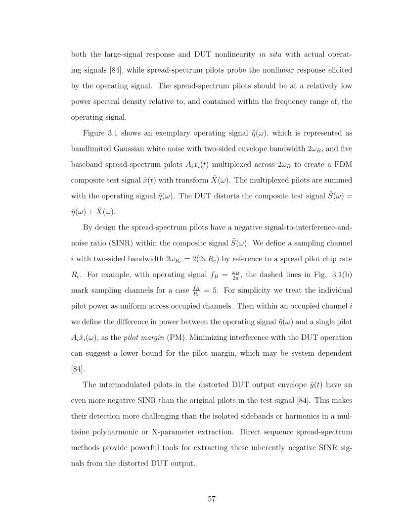
both the large-signal response and DUT nonlinearity in situ with actual operat-
ing signals [84], while spread-spectrum pilots probe the nonlinear response elicited
by the operating signal. The spread-spectrum pilots should be at a relatively low
power spectral density relative to, and contained within the frequency range of, the
operating signal.
Figure 3.1 shows an exemplary operating signal η(ω), which is represented as
bandlimited Gaussian white noise with two-sided envelope bandwidth 2ωB, and five
baseband spread-spectrum pilots Aixi(t) multiplexed across 2ωB to create a FDM
composite test signal x(t) with transform X(ω). The multiplexed pilots are summed
with the operating signal η(ω). The DUT distorts the composite test signal S(ω) =
η(ω) + X(ω).
By design the spread-spectrum pilots have a negative signal-to-interference-and-
noise ratio (SINR) within the composite signal S(ω). We define a sampling channel
i with two-sided bandwidth 2ωRc = 2(2πRc) by reference to a spread pilot chip rate
Rc. For example, with operating signal fB = ωB
2π, the dashed lines in Fig. 3.1(b)
mark sampling channels for a case fBRc
= 5. For simplicity we treat the individual
pilot power as uniform across occupied channels. Then within an occupied channel i
we define the difference in power between the operating signal η(ω) and a single pilot
Aixi(ω), as the pilot margin (PM). Minimizing interference with the DUT operation
can suggest a lower bound for the pilot margin, which may be system dependent
[84].
The intermodulated pilots in the distorted DUT output envelope y(t) have an
even more negative SINR than the original pilots in the test signal [84]. This makes
their detection more challenging than the isolated sidebands or harmonics in a mul-
tisine polyharmonic or X-parameter extraction. Direct sequence spread-spectrum
methods provide powerful tools for extracting these inherently negative SINR sig-
nals from the distorted DUT output.
57

(a)
(b)
Figure 3.1: Test signal S design given operating signal η modeled as bandlimited Gaussian white noise, andpilots X =
∑i Aixi: (a) baseband test signal generation and injection at DUT, showing cubic distortion
envelope; (b) test signal envelope detail, with dashed lines marking channels associated with each pilot.[From [84].]
58

Spread pilots resemble noise from the DUT viewpoint [87, 89]. The requirement
that the pilots minimally perturb the DUT operation further implies that the pilots
X(ω) must be uncorrelated with the operating signal η(ω). If we model our rep-
resentative operating signal as bandlimited Gaussian white noise, then duobinary
maximal length pseudorandom (PN) sequences (m-sequences) provide a good start-
ing point for system measurement pilots. Pulse shaping can bandlimit the pilots in
a manner that facilitates the baseband multiplexing as shown in Fig. 3.1(b) [84].
In short, measuring nonlinearity responding to a dominant operating signal, and
only minimally perturbed by spread probing signals, suggests spread-spectrum meth-
ods based on pulse-shaped PN sequence pilots. The PN chip rate is chosen to define
a desired number of sampling channels spanning the operating signal bandwidth. A
fixed positive power margin should be preserved between the operating signal and pi-
lot in each channel, leading to inherently negative SINR for nonlinear identification,
which can be overcome by the processing gain of the system.
3.2.2 Designing pilots for nonlinear measurements
For nonlinear kernel measurement the pilot design must ensure orthogonality among
the intermodulated codes resulting from nonlinear operation on the multiplexed pilot
envelope x(t). By inspection, however, the intermodulation products include two
types of correlated results that require attention in the code design.
The first, which we call a systematic correlation, concerns the correlation of cer-
tain cubic distortion terms (involving third-order self-modulation distortion (SMD3)
and cross-modulation distortion (XMD3)) with the first-order DUT output. As
shown below, this well-known result from harmonic distortion theory [96] also ap-
plies to the intermodulation code products, insofar as these cubic distortion terms
contribute correlated signal on the linear output term. The converse, however, does
not hold, as the cubic distortion terms can be designed so that they include inter-
59

modulation coding that remains orthogonal to the DUT linear output (as well as
each other distortion term).
The second correlated intermodulation distortion is more subtle. This problem
takes two forms, which we describe under the heading of pseudorandom correlation.
The problem lies in the binary product (XOR) of three (or more) duobinary maximal-
length pseudorandom (PN) sequences (in a nonlinearity with or without memory),
rather than the polynomial expansion of a no-memory nonlinearity that introduces
systematic correlation. As discussed further below, the defining properties of the PN
sequence [88] mean that the intermodulating bitwise binary multiplication of three or
more distinct PN sequences can produce the same PN sequence as an intermodulated
code resulting from another set of PN sequences. We call this event a code collision.
A code collision involving the intermodulation code adds correlated noise on the
intermodulation distortion (the signal for the coefficient measurement) that distorts
the coefficient estimate when that intermodulation code is used as an argument in
nonlinear parameter extraction.
The code collision includes a special case in which the intermodulation product of
two PN sequences results in the third PN sequence in an intermodulation product (for
a cubic distortion). We call this case an intermediate code collision (more properly,
a failure of the conditions needed to apply the shift-and-add property [88]). The
intermediate code collision introduces a DC term in the distortion products and
makes the associated intermodulation code inoperable as a correlation argument.
Given these considerations the code design proceeds as follows. The code is
optimized for measuring nonlinear distortion subject to unavoidable systematic cor-
relation on the DUT linear output (or distortion terms having order less than the
nonlinearity). This design is subject to additional steps to avoid code collisions in
the DUT output.
60

3.2.2.1 Systematic intermodulation
Wemodel the discretized first-zone DUT output envelope in Fig. 3.1a with a lowpass-
equivalent quasi-memoryless cubic polynomial
y(n) = h1x(n) + h3x(n) (x∗(n)x(n)) (3.1)
with complex coefficients h1,3. x(n) is the test signal aggregating multiplexed spread
pilots Aqxq, q ∈ [1, Q] for Q pilots as shown in Fig. 3.1b, and ∗ notes complex
conjugation. The amplitude Aq relates to relevant spread coding element magnitudes
as described further below.1 Probing individual distortion terms, we can write the
quasi-memoryless third-order nonlinear distortion envelope due to mixing particular
pilots at ijk channels as
yijk(n) = AiAjAkhijk3 xi(n) (xj(n)x
∗k(n)) , (3.2)
(i, j, k) ∈ [1, Q].
The superscript pilot indices track the distortion term provenance. The channel i
envelope component associated with the linear (first-order) DUT response is yi(n) =
Aihi1xi(n).
For a cubic distortion we can define a distortion taxonomy in terms of the pi-
lots that contribute to a particular distortion term. A cubic nonlinearity generates
four distinct distortion types that we call self-modulation (SMD3), cross-modulation
(XMD3), intermodulation (IMD3), and triple product (TPD3) distortions, falling
at f , with phase ϕ, scaled by amplitude A, according to the rules shown in Table
2.1, using the pilot index as shorthand for the associated channel frequency. This
1The third-order quasi-memoryless Volterra series is introduced in order to provide context for thecode design problem. The code design and correlation-based nonlinear identification methodol-ogy using those spread codes can be extended to memory polynomials or other Volterra seriestruncations with memory.
61

Table 3.1: Third-order distortion terms.
Type Rule f ϕ A
SMD3 i = j = k i ϕi A3i
XMD3i = j, j = ki = j, i = k
ij
ϕi
ϕj
A2jAi
A2iAj
IMD3 i = j, j = k 2i− k 2ϕi − ϕk A2iAk
TPD3i = j, i = k,
j = ki+ j−k
ϕi + ϕj
−ϕkAiAjAk
framework will specify the third-order spread pilot combinations that generate the
intermodulated code sequences for any given distortion term.
Suppose we define the spread pilots Aixi(n) in channel i as maximal length
duobinary BPSK-coded PN sequences with primitive polynomial of degree r over
GF(2) and code length (period) N = 2r − 1. With a given initial condition the
primitive polynomial specifies a reference sequence c. We define M orthogonal PN
sequences cm = T pmc with a chip offset or phase pm from c and m ∈ [1, 2, . . . ,M ],
M ≤ N .
In order to unambiguously measure the nonlinearity, we want to identify a spread
pilot sequence that, applied to a DUT, results in orthogonal coded distortion terms.
If we restrict our attention to simple additive combinations, this requires combining
multiple PN sequences. To see this, consider the case of third-order distortion and
a single baseband pilot c1 centered on DC. As shown in Table 3.1, the cubic dis-
tortion for this pilot alone is third-order self-modulation distortion (SMD3), whose
magnitude we want to identify.
With a single BPSK-encoded PN sequence the third-order distortion at the DUT
output is proportional to the intermodulated coding (IC). Suppressing the time in-
62

dex, the cubic IC in this case is
IC = c1(c1∗c1
)(3.3)
= c1,
using c(n) · c(n) = 1, ∀n ∈ [0, N − 1].
We reject this single PN sequence as the spread coding for kernel extraction be-
cause the intermodulated code is indistinguishable from the undistorted, linear code
c1. In other words, this code choice cannot distinguish the cubic intermodulation
distortion from the first-order DUT output.
The same result holds for other simple PN sequence combinations. Suppose we
take the sum of two real PN sequences, a = c1 + c2. The cubic intermodulated code
is
IC =(c1 + c2
) (c1 + c2
)∗ (c1 + c2
)(3.4)
=(c1 + c2
) (|c1|2 + 2c1c2 + |c2|2
)=(c1 + c2
) (2 + 2c1c2
)= 4
(c1 + c2
).
This intermodulated code, in other words, is also a scaled version of the undistorted
spread pilot and cannot distinguish cubic distortion from linear DUT output (e.g.,
a scaling and rotation in a given channel).
Table 3.2 collects the cubic intermodulation products for a range of possible PN
combinations. Prior efforts at identifying nonlinear kernels of RF systems using
spread-spectrum coding relied on single-carrier test signals compiled from forward
link CDMA inputs [80, 81, 83]. These spread-spectrum codes resembled those used
in [82]. The fourth row in Table 3.2 provides a species of the coding described in
63
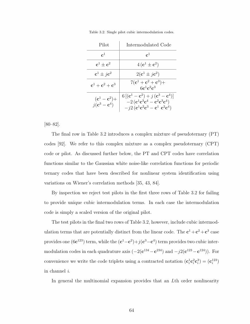
Table 3.2: Single pilot cubic intermodulation codes.
Pilot Intermodulated Code
c1 c1
c1 ± c2 4 (c1 ± c2)
c1 ± jc2 2(c1 ± jc2)
c1 + c2 + c37(c1 + c2 + c3)+
6c1c2c3
(c1 − c2)+j(c3 − c4)
6 [(c1 − c2) + j (c3 − c4)]−2 (c1c3c4 − c2c3c4)−j2 (c1c2c3 − c1 c2c4)
[80–82].
The final row in Table 3.2 introduces a complex mixture of pseudoternary (PT)
codes [92]. We refer to this complex mixture as a complex pseudoternary (CPT)
code or pilot. As discussed further below, the PT and CPT codes have correlation
functions similar to the Gaussian white noise-like correlation functions for periodic
ternary codes that have been described for nonlinear system identification using
variations on Wiener’s correlation methods [35, 43, 84].
By inspection we reject test pilots in the first three rows of Table 3.2 for failing
to provide unique cubic intermodulation terms. In each case the intermodulation
code is simply a scaled version of the original pilot.
The test pilots in the final two rows of Table 3.2, however, include cubic intermod-
ulation terms that are potentially distinct from the linear code. The c1+c2+c3 case
provides one (6c123) term, while the (c1−c2)+j(c3−c4) term provides two cubic inter-
modulation codes in each quadrature axis (−2(c134−c234) and −j2(c123−c124)). For
convenience we write the code triplets using a contracted notation (c1i c2i c
3i ) = (c123i )
in channel i.
In general the multinomial expansion provides that an Lth order nonlinearity
64

applied to M PN sequences spread across Q channel pilots results in
M + L− 1
L
intermodulation terms. Among those terms,
M
L
will consist of intermodulated
code products involving L distinct PN sequences. In a cubic nonlinearity the re-
maining intermodulation codes are necessarily products of at least two identical PN
sequences. The XOR of the two identical BPSK coded PN sequences reduces to an
Nx1 vector of ones, so that the resulting intermodulation code product will be iden-
tical to the third sequence in the product, meaning identical to one of the sequences
used to generate the underlying pilot.
These intermodulation distortion code terms are not useful for nonlinear identi-
fication. In general, the number of distinct PN codes used to form the pilot must be
at least as large as the nonlinear order being investigated, e.g., M ≥ L. The number
of sequences used to form the spread pilot, in other words, must be at least the same
as highest nonlinear order [81].
The shift-and-add property guarantees that for integers i and j, i = j and 0 ≤
i, j < N , ∃ k = i, j with 0 ≤ k < N such that T ic⊕
T jc = T kc [88]. In other
words, the XOR of two m-sequences with distinct phases from the same primitive
polynomial is another m-sequence in the same code space. Applying this property
twice means that the intermodulated code triplets in Table 3.2 are themselves m-
sequences from the same N -dimensional code space as c.
3.2.2.2 Nonlinear identification with multiple pilots
Nonlinear identification code design requires ensuring that the code triplets in the
cubic intermodulation code products remain orthogonal to all the other intermod-
ulation code products, including the m-sequences forming the undistorted pilot.
Code triplets in this sense means the XOR of three different PN sequences (e.g.,
65

c1c2c3 = c123). When we add more pilots, at more frequencies, the resulting code
triplets need to remain orthogonal to other intermodulated code terms that will
have frequency components overlapping the spectrum for the intermodulated code
of interest. For this systematic intermodulation discussion we will assume, for argu-
ment, that the code triplet orthogonality can be ensured by suitable choice of the
underlying code phases pm for m ∈ [1,M ] distinct PN sequences.
To make this issue more concrete, assuming that the code triplets that result
from intermodulating a single pilot are orthogonal m-sequences, then these code
triplets (3-tuples) are candidate correlation arguments for identifying the complex
coefficient, or kernel, associated with the nonlinearity for those pilot frequencies. For
example, taking c234 as a correlation argument against the distorted output, from
the last row in Table 3.2, with a = (c1 − c2) + j(c3 − c4) and using the well-known
correlation properties of PN sequences [88],
< (aiaia∗i ),c
234i > (3.5)
= < 6[(c1i − c2i ) + j(c3i − c4i )], c234i >
− < 2(c134i − c234i ), c234i >
− < j2(c123i − c124i ), c234i >
= 6(−1− (−1)) + j(−1− (−1))
−2(−1−N)
−j2(−1− (−1))
= 2(N + 1).
We set the amplitudes Aq in (3.2) as the magnitude of individual PN sequences c
in the combinations in Table 3.3. Now using this correlation on the DUT distor-
tion product we can identify the kernel, or complex coefficient hijk3 , that scales the
nonlinear output envelope for these pilot combinations in (3.2).
66

Turning back to the last two rows of test codes in Table 3.2 as possible candi-
dates for identifying bandpass nonlinearities, we observe that the real sum of three
BPSK PN sequences (c1 + c2 + c3) has a quaternary alphabet with amplitudes of
−3,−1, 1, 3. Without pulse shaping the peak to average power ratio (PAPR) for
a single test pilot based on this sequence is ∼ 4.8 dB, with signal power in only one
quadrature axis.
The last test pilot in Table 3.2 can be rewritten a = a1 + ja2, where a1 = (c1 −
c2) and a2 = (c3 − c4) are pseudoternary (PT) codes [92]. Each pseudoternary code
has an alphabet −2, 0, 2, and without pulse shaping the complex pseudoternary
(CPT) pilot based on this sequence has PAPR ∼ 3 dB in each quadrature axis.
Unlike the real sum of three PN sequences, the CPT pilot has equal signal power
in each quadrature axis. The lower PAPR can become significant as the number of
multiplexed pilots in a test signal increases.
For this application several features make the CPT pilot superior to the sequence
sum in Table 3.2 row 4, and [80–82]. The CPT pilot has better spread code noise
rejection than the real PN sum pilot. Correlating on an underlying PN sequence
provides comparable correlation peak values: the CPT pilot provides < (c1 − c2) +
j(c3 − c4), c1 >= N + 1, while the triple sum pilot provides < (c1 + c2 + c3), c1 >=
N−2. With an uncorrelated sequence c5 = T p5c, however, the CPT pilot correlation
provides a null < (c1−c2)+j(c3−c4), c5 >= 0 while the real PN sum pilot provides
nonzero spread code noise < (c1 + c2 + c3), c5 >= −3.
The spread code noise rejection improvement for CPT codes also holds for cor-
relation on the associated intermodulation products. For CPT code a = (c1 − c2) +
j(c3−c4), < (aaa∗), c234 >= 2(N +1), and < (aaa∗), c5 >= 0, while for the real PN
sum pilot a = c1 + c2 + c3, < (aaa∗), c123 >= 6N − 21 and < (aaa∗), c5 >= −27.
Because of its generally preferable spread code noise values, lower PAPR and even
power distribution in the real and quadrature signal axis, we will focus our attention
67

Table 3.3: Cubic intermodulation codes by distortion type.
Type Rule Intermodulated Code
SMD3i = jj = k
ai(a∗iai) =
6i [(c1 − c2) + j (c3 − c4)]−2 · (c1i c3i c4i − c2i c
3i c
4i )
−j2 ·i (c1i c2i c3i − c1i c2i c
4i )
XMD3i = jj = k
ai(a∗jaj) =[4(c1i − c2i )− 2(c12j + c34j )(c1i − c2i )
]+j[4(c3i − c4i )− 2(c12j + c34j )(c3i − c4i )
]
IMD3i = ji = k
(aiai)(a∗k) =
2 [(c3i c4i − c1i c
2i )(c
1k − c2k)
+(c1i − c2i )(c3i − c4i )(c
3k − c4k)]
−j2 [(c3i c4i − c1i c
2i )(c
3k − c4k)
−(c1i − c2i )(c3i − c4i )(c
1k − c2k)]
TPD3i = ji = kj = k
(aiaj)a∗k =[
(c1i − c2i )(c1j − c2j)(c
1k − c2k) + . . .
]+j[. . .− (c1i − c2i )(c
1j − c2j)(c
3k − c4k)
]on the CPT pilot for nonlinear identification.
Now instead of a single pilot, suppose we allowQ ≥ 3 CPT pilots ai, aj, ak, i, j, k ∈
[1, Q] distributed in Q channels across the baseband as in Fig. 3.1. The first-zone
cubic distortion products have the general form aiaj(a∗k) as described in Table 2.1.
Table 3.3 gives the resulting intermodulation code terms for third-order distortion on
CPT pilots. The intermodulated code for each distortion contains several candidate
code-tuples, in phase and quadrature, which can be used as correlation arguments.
Only one orthogonal correlation argument is strictly needed to identify the associ-
ated distortion coefficient for a given channel and pilot combination. For the kernel
identification, the unused intermodulated code terms are simply redundant. The
CPT pilots are in this sense somewhat inefficient, since nonlinear DUT intermodu-
68

lation spreads signal energy to unused intermodulated code terms. This inefficiency,
however, is inherent in the tendency of nonlinear distortion to spread signal energy
in frequency and code space.
Finally, Table 3.3 shows that the SMD3 and XMD3 intermodulated code terms
include scaled versions of the original CPT pilot. For example, XMD3 contains a
4 ((c1i − c2i ) + j(c3i − c4i )) term, which is a scaled version of the i CPT pilot. This
means that the SMD3 and XMD3 distortions generate correlated, coded signal on
the first-order transfer. The remaining SMD3 and XMD3 intermodulation terms,
however, are orthogonal to the PN sequences in the underlying CPT pilot. For
kernel identification purposes, this means that we can uniquely identify the highest-
order distortion coefficients by correlation on the distorted DUT output envelope.
The linear kernel identification is indirect insofar as it requires first identifying, then
subtracting, the systematic coded correlated cubic distortion from the SMD3 and—
when there are 2 or more pilots—the XMD3 distortion term. In most cases, the
potential error that might result from this subtraction is very small [84].
3.2.2.3 Avoiding code collision
The shift-and-add property guarantees that the triple code products in the inter-
modulated code terms are themselves m-sequences in the same code space as the
underlying PN sequences, but says nothing about the exact phase of the resulting
code products.
In terms of cubic intermodulation we want to specify Q = 4M PN sequences in
terms of the phases for the underlying PN sequences using cqi = T pi,qc with q ∈ [1, 4]
marking the PN location in the complex pseudoternary sequence mixture for the
CPT pilot in channel i ∈ [1,M ].
To simplify the notation for any three PN triplets, in this discussion we will use
generic indices to represent the code phase. Then for three PN sequences having
69

phase i, j, k, i = j = k, cijk = T ic⊕ T jc⊕ T kc, we can break the bitwise product
(sequence XOR) into parts
cij = T ic⊕ T jc = Tmc, (3.6a)
cijk = Tmc⊕ T kc = T pc, m = k. (3.6b)
Determining the result of the code intermodulation for use in a correlation on a
received signal requires ascertaining the resulting phase for a given the code triplet
cijk. Note that the shift-and-add property requires that the resulting intermediate
code product phase is itself different from the final code phase in the triple product,
so that the intermodulated code triplet will be an m-sequence from c.
This process is visualized in Fig. 3.2, where code space S is the set of N orthog-
onal PN sequences defined by the binary generating polynomial with degree r. The
Q CPT pilots consist of M = 4Q PN sequences drawn from the code space S. A1
is the set of M = 4Q orthogonal PN sequences comprising the Q CPT pilots, and
A2 ⊂ A1 is the set of the correlation arguments for linear kernel extraction. B is the
set of(M3
)code triplets comprised of distinct PN sequences in the resulting inter-
modulation terms, excluding the systematic correlated terms (linear codes) from the
SMD3 and XMD3 distortions (e.g., i = j, k = i, j). B ∪A1 is the set m-sequences
in the DUT output envelope.
The code collision problem concerns intermodulated code duplication. C ⊂ B is
the set of intermodulation code triplets selected as correlation arguments for cubic
kernel extraction. The code orthogonality condition for the cubic distortion correla-
tion arguments can be written as C ∩ B \ C = ∅, while for the linear distortion
correlation arguments we require B ∩A2 = ∅. In other words, given a set of distinct
intermodulated code triplets for correlation arguments, it is necessary that no other
intermodulation products duplicate the phase for any code in C ∪ A2. Violating
70

Figure 3.2: Intermodulation code triplet generation. S is the code space size N = 2r − 1 for Q CPT pilotsfrom primitive polynomial degree r over GF(2). A1 is the set of m-sequences used in all Q CPT pilots,A2 ⊂ A1 is the set ofm-sequences used for linear kernel extraction. B is the set of intermodulated code termsin the DUT output envelope excluding the correlated linear codes from the SMD3 and XMD3 distortions(e.g., i = j, k = i, j), so that A = A1 ∪B is the set of m-sequences in the DUT output envelope. C ⊂ Bis the set of intermodulated code triplets in the DUT output envelope selected as correlation arguments forcubic distortion kernel identification.
these conditions results in correlated noise that will distort the corresponding kernel
estimate based on the correlation output.
In order to avoid code collision, we test safe m-sequence combinations by screen-
ing the intermodulation products for initial PN phases in A1. Testing for these
code collisions could involve an exhaustive search among all code intermodulated
possibilities—an enormous list. To improve the search, it is helpful to consider the
XOR operation with reference to the initial LSFR state for sequence u.
Observing that the cyclical left-shift operator is distributive over the XOR oper-
71

Table 3.4: LFSR States For r = 3 m-sequence.
i Q3 Q2 Q1
0 0 0 1
1 0 1 0
2 1 0 0
3 1 0 1
4 1 1 1
5 0 1 1
6 1 1 0
ation. we can premultiply (3.6a) by a null shift T iT−i,
T ic⊕ T jc= T iT−i(T ic⊕ T jc
)= T i
(c⊕ T (j−i)c
)= Tmc. (3.7)
This expresses the intermediate code product phase m in terms of any two code
phases (i < j) and an XOR referenced to the initial code c.
In order to apply this result to reduce the code search, we construct a N × r
matrix of the shift register states (which we call the state matrix ) for codes T ic
with 0 ≤ i ≤ N − 1, where each row advances the register and code phase by one
state. The LSFR register states are the vector representation of the polynomial basis
(αi), i ∈ [0, ..., N −1] used to construct GF (2r) from the irreducible polynomial f(x)
of degree r over GF (2) [91].
For exposition Table 3.4 shows a representative state matrix for a third-degree
m-sequence LFSR with a primitive polynomial f(x) = x3 + x2 + 1 of degree r = 3
over GF (2) [87, 90]. The code length is N = 23 − 1 = 7 bits.
Next we construct an auxiliary (N − 1) × r matrix (the product state matrix )
for 1 ≤ j ≤ N − 1, with each row being the XOR of the register state (tabulated
72

Table 3.5: Product State Matrix and Product Shift Vector.
j Q3 Q2 Q1 m
1 0 1 1 5
2 1 0 1 3
3 1 0 0 2
4 1 1 0 6
5 0 1 0 1
6 1 1 1 4
in the state matrix row vectors) for the c and T jc sequences. Table 3.5 shows a
representative product state matrix for the state matrix in Table 3.4.
For a given LFSR state j, the XOR with the initial LFSR state (i = 0) results in
a third LFSR register state associated with the shifted code product c⊕T jc = Tmc.
Locating the LFSR state in the state matrix provides the associated shift m. We
form an (N − 1)× 1 product shift vector m associating each product phase mj with
the offset phase j, 1 ≤ j ≤ N − 1, used in the code product.
The final column in Table 3.5 shows an exemplary product shift vector m for the
LFSR state matrix in Table 3.4. The vector m is also the trinomial table τ(i) where
1+αi = ατ(i) for the vector representation of the polynomial basis in Table 3.4 [91].
Now given any two codes with phases i < j, we identify the shift associated with
c⊕T (j−i)c from the product shift vector m, and add i to identify the shift associated
with T ic⊕ T jc = T i(c⊕ T (j−i)c).
We give a numeric example of this calculation using Tables 3.4 and 3.5. For
degree r = 3 the m-sequence primitive polynomial over GF(2) is f (x) = x3 + x2 +1
and the initial condition is (001) [90]. In terms of the vector representation, α0 = 1
and αi = 0 ∀i ∈ [1, ..., N − 1] [91].
Consider an example, such as T 2c⊕ T 5c. Using Table 3.4, computing the XOR
directly in state space provides (100)⊕ (011) = (111). By inspection Table 3.4 shows
73

that the sequence with register state (111) is T 4c, so T 2c⊕T 5c = T 4c. This matches
the result by XOR on the literal code sequences themselves, (1110100)⊕(0100111) =
(1010011).
By comparison, the shift calculation using the product state matrix is more
computationally efficient. Using Table 3.5, we find c ⊕ T (5−2)c = T 2c. In the
preceding notation, j = 3 and m3 = 2. Adding i = 2 provides, as expected, i+m3 =
2 + 2 = 4 and T 2c⊕ T 5c = T 2 (c⊕ T 3c) = T 2 (T 2c) = T 4c.
Another example demonstrates the duplicate phase or code collision problem.
Consider two code triplets, T 0c⊕ T 3c⊕ T 4c and T 0c⊕ T 2c⊕ T 6c. Both triplets in-
volve orthogonal m-sequences, with phases 0, 3, 4 and 0, 2, 6. Both code triplets,
however, result in the same sequence T 5c. Reducing the first triplet,
T 0(c⊕ T 3c) = T 2c, (3.8a)
T 2c⊕ T 4c = T 2(c⊕ T (4−2)c)
= T 2(T 3c) = T 5c (3.8b)
and the second triplet,
T 0(c⊕ T 2c) = T 3c, (3.9a)
T 3c⊕ T 6c = T 3(c⊕ T (6−3)c)
= T 3(T 2c) = T 5c. (3.9b)
The duplication would introduce a code collision if either triplet, (c⊕ T 2c⊕ T 5c) or
(c⊕ T 2c⊕ T 6c), were used as a correlation argument for kernel extraction.
Note that T 0c⊕T 2c⊕T 3c—another code triplet also involving three orthogonal
sequences—provides an intermediate code collision, or the XOR of the intermediate
distortion product with itself. The second XOR violates the shift-and-add condition
74

on T ic⊕T jc that i = j. Distortion triplets with intermediate code collision add DC
to the channel envelope, and like code collision, add noise to the correlation-based
kernel estimates. The code triplet with intermediate code collision is inoperative as
a correlation argument.
We apply these tools to anticipate and eliminate the potential for code collision
as follows. First, we set the code degree r and number of pilots (channels) Q that will
be used to probe the cubic DUT nonlinearity [84]. Second, we form the associated
state matrix, product shift vector m, and product state matrix for the code order r.
These look-up references are generated once per code order r.
Given Q CPT pilots with code order r, we need to specify the particular phases
pi,j, i ∈ [1, Q], j ∈ [1, 4] for the 4Q constituent PN sequences. For reasons relating
to code acquisition discussed below, for cji = T pi,jc we constrain pi,2 = pi,1 + 1,
pi,4 = pi,3 + 1, and (|pi,3 − pi,1|) > 3 [92]. This leaves 2Q free code phases. Rather
than catalog the safe codes for r,Q combinations, we search by randomly seeding
the free code phases subject to 0 ≤ pj < N and rankp = 4Q.
Next we identify the correlation arguments C ∪ A2 that will be used for kernel
extraction from the DUT output [84]. Using the methodology described above, for
each random code seeding we test each code triplet correlation argument to ensure
1) no intermediate code collision (each intermediate product phase is distinct from
the final code phase), and 2) no code collision with each other member of C ∪ A2.
Assuming no conflict, given Q we identify each unique intermodulated code triple
product in the DUT output for each distortion combination in Table 3.3 [84]. This
gives us B. Now we test each code triplet in B \ (C ∪A2) to verify no collision with
the correlation arguments in C ∪ A2.
If we encounter a collision or intermediate code collision condition, we repeat the
search with a new random code seeding. If the test completes without encountering
conflict, then the test seed coding can be used with cubic distortion kernel extraction
75

without intermediate code collision or code collision [84].
The number of random trials needed before identifying suitable code phase seed-
ing is inversely proportional to the degrees of freedom in the intermodulated code
terms, which relates to the code order r (and code length N) and the number of
channels Q. In the memoryless case with Q channels and CPT pilots, the number
of distinct code triplets in the intermodulated output is no more than(4Q3
), while
the code space S has size N . When the number of intermodulation products ex-
ceeds the size of the code space S some set of code triplets must result in duplicate
phases, although not necessarily duplicate phases within C ∪ A2, which introduces
the unwanted pseudorandom correlated noise. The larger the code space—meaning
the higher the code order r and the longer the m-sequences—the greater the choice
of code phases in the seed codes and the lower the probability of a intermediate
code collision in the intermodulated code terms or a collision with the correlation
arguments.
In relation to the number of code triplets or code space size, the number of cor-
relation arguments grows much more slowly. If we intend to identify the memoryless
third-order nonlinear kernel for each distortion in each pilot-occupied channel, then
the minimum number of correlation arguments will never be larger than 5Q. For
code order r = 20 and five pilots (Q = 5), safe seed codes can be identified in a
handful of trials, whereas a low code order r = 10 with three pilots (Q = 3) may
require closer to 1,000 trials.
While we have described the process for CPT pilot design for memoryless cubic
distortion kernel extraction, the same process can be also applied to verify safe code
phase seeding for the complete memory polynomial model of (E.2) [84]. In this case,
the search has to additionally encompass the nearby codes associated with the delay
of the DUT.
76

3.2.3 Code acquisition
The system must determine the code alignment in the received signal before it can
extract kernels by correlation against the intermodulation code terms. While there
are several code acquisition and tracking methodologies for BPSK-encoded data, it
is not clear that CPT pilot acquisition has been deeply explored. Reference [92] ob-
served that pseudoternary pilots themselves have autocorrelations that can improve
bit error rates.
The PT pilot autocorrelations can be evaluated using the periodic crosscorre-
lation properties of the constituent m-sequences. Take c1 = T p1c and c2 = T p2c
with p2 = (p1 + 1). We can write, < (c1 − c2), (c1 − c2) >=< (c1 − c2), c1 > − <
(c1 − c2), c2 >. The first periodic correlation is
< (c1 − c2), c1 > = < T p1(c− T 1c), T p1c > (3.10)
=N−1∑n=0
T p1(c− T 1c)⊕ T nc
=
N + 1, n = 0,
−(1 +N), n = 1,
0, else.
The second periodic correlation is similarly,
< (c1 − c2), c2 > = < T p1(c− T 1c), T p1+1c > (3.11)
=N−2∑n=−1
T p1(c− T 1c)⊕ T 1+nc
=
(N + 1), n = −1,
−(N + 1), n = 0,
0, else.
77

Figure 3.3: Pseudoternary sequence normalized periodic autocorrelation.
Combining (E.14) and (E.15) provides a periodic autocorrelation with a single max-
imum. The periodic autocorrelation is identically zero more than one chip from
alignment,
θc1−c2,c1−c2(n) = (3.12)
−(N + 1), n = −1
2(N + 1), n = 0
−(N + 1), n = 1
0, else.
Fig. 3.3 shows the normalized periodic autocorrelation detail for the pseu-
doternary pilot. The delay associated with the secondary peak autocorrelations
−(N + 1) are determined by the relative phases in the m-sequences c1 and c2 in the
pseudoternary code, in this case set to 1. The pseudoternary autocorrelation mimics
78

Figure 3.4: Offset spectrum for orthogonal pulse-shaped CPT pilots X(f) with chip rate Rc = 1 MHz inbaseband at −4, 2, 0, 2, 4 MHz with B = 5 MHz bandlimited operating signal η(f) at 20 dB pilot margin.Dashed lines mark the central (zero offset) channel. (Compare Fig. 3.1.)
the periodic ternary autocorrelation from an m-sequence in a third-order Galois field
[35, 43]. The periodic pseudoternary autocorrelation is zero-mean, resulting in a DC
null in the power spectral density.
Fig. 3.4 shows a representative spectrum for five CPT pilots, with chip rate Rc =
1 MHz, subject to raised-cosine filtering with excess bandwidth α = 0.22. After pulse
shaping the CPT pilots are multiplexed in the baseband at −4,−2, 0, 2, 4 MHz.
The CPT pilots are shown with a 20dB pilot margin (PM) compared to operating
signal η with two-sided bandwidth 2B = ∼ 10 MHz. The PM is defined as
PM = −10log10
(var(F ∗ xi(t)) ·Bvar(η(t)) ·Rc
)(3.13)
with F the impulse response for a unit amplitude brickwall channel filter with two-
sided bandwidth 2Rc.
Conventional correlation maximization strategies have some limitations for code
79

acquisition using the proposed complex pseudoternary pilots, although they can be
used for “real” pseudoternary pilots alone [92]. To see this, for a given channel q write
the CPT pilot aq = a1q + ja2
q, with a1q = T pq,1c− T pq,1+1c and a2q = T pq,2c− T pq,2+1c
subject to the constraints described above. More generally, we can write ajq =
T pq,j(c− T 1c), j ∈ 1, 2.
Any rotation θ by the signal path through the DUT or the nonlinear distortion
projects some portion of the in-phase pseudoternary pilot a1 onto the quadrature
axis, and some portion of the quadrature pseudoternary pilot a2 onto the in-phase
axis,
a · exp(jθ) = (a1 + ja2)(cos(θ) + jsin(θ)) (3.14)
=
[a1cos(θ)− a2sin(θ)
]+j
[a1sin(θ) + a2cos(θ)
].
In a typical test environment, unfortunately, we have no a priori information about
the received signal rotation θ.
Except where an accumulated phase is an integer multiple of π and nulls the
complementary axis projection on the in-phase or quadrature signal, correlation
against the pseudoternary pilot on the axis of interest returns a local maximum
associated with each CPT pilot component. As an example, let us evaluate the
autocorrelation of the in-phase received (and rotated) signal against the in-phase
pseudoternary code a1, where the received in-phase signal has components of both
a1 and a2. Suppose p2 > p1. Then T (p2−p1)T p1(c1 − T 1c1) = T p2(c1 − T 1c1) = a2.
In other words, at shift n = (p2 − p1) away from the correct code alignment, the
correlation argument for the cross-correlation on the in-phase signal is converted
to the quadrature pilot, and the cross-correlation output reports a“false alignment”
resulting from the quadrature pilot projection in addition to the “correct” alignment
80

peak from the in-phase projection. The same effect applies to the quadrature signal.
The false alignment peaks on the in-phase and quadrature cross correlations move
in opposite directions, relative to the correct alignment mark.
If we consider both the in-phase and quadrature signal autocorrelations against
their respective pilots, we see that except for a π2, 3π
2rotation, the I and Q autocor-
relations always have coincident delay peaks at the code alignment, in addition to
non-coincident peaks resulting from the phase rotation.
This suggests that, for best performance, code acquisition should maximize the
product of the received I and Q signal crosscorrelations with their respective pseu-
doternary pilots. For completeness, to exclude the case of a π2, 3π
2phase accumulation
we can also include the product of I and Q autocorrelations subject to unequal phase
dithers on the received signal, such as π4, π
8. With the dither, at least two of the
autocorrelation products must be nonzero at the code alignment.
We applied this methodology using CPT pilots in the coherent direct sequence
spread-spectrum nonlinear identification system described in [84]. The pilots are
combined with an operating signal, injected at the DUT input, with the intermod-
ulated codes evaluated at the DUT output.
We divide the code acquisition process into a coarse and fine alignment. Although
we sample at a rate much higher than the chip rate, for the coarse alignment we max-
imize the product of the I and Q pseudoternary pilot autocorrelations at the chip
rate. Once we have the coarse alignment to within a chip, we can maximize the auto-
correlation magnitude on one axis (in-phase) to find the channel code alignment—if
desired—to within a sample, or Rc
fsof a chip for chip rate Rc and sample rate fs.
Fig. 3.5 shows code acquisition measured for long CPT codes with degree r = 20
at arbitrary delays for one of five representative channels, with a 20 dB pilot margin.
The CPT pilots have chip rate Rc = 1 MHz, located at −4,−2, 0, 2, 4 offset in
the baseband as shown in Fig. 3.1, prior to combining with the operating signal,
81

Figure 3.5: Measured code acquisition for r = 20, channel 3 of 5, with pilot margin 20 dB. Accumulatedphase is nearly an integer multiple of π.
multiplexed to fLO = 1960 MHz and injected at the DUT [84]. Pilots are pulse
shaped with raised cosine filtering [84]. As discussed in the text, each CPT consists
of orthogonal pseudoternary pilots with fixed phase offset of one chip between m-
sequences. The seed code phases were selected using the methodology outlined in
the previous subsection, resulting for each channel in different offsets between CPT
in phase and quadrature pseudoternary codes.
The top panel in Fig. 3.5 shows the in phase received signal correlation against
the associated pseudoternary pilot, RI(n); the middle panel shows the quadrature
received signal correlation against its associated pseudoternary pilot, RQ(n); and
the third panel shows the product of the two RI(n) · RQ(n) with peak at the code
alignment. A dotted line marks the measured true alignment in each panel, in
samples from the data capture start.
The absolute phase, or signal rotation, at each data capture is arbitrary. Since
we use a coherent detector, the phase accumulation per channel reflects individual
channel dispersion as well as any residual jitter between the signal generating PLL
per I and Q channel at the AWG, and the ADC PLL per I and Q channel in the 16
82

Figure 3.6: Measured code acquisition for r = 20, channel 2 of 5. Accumulated phase is nearly an integermultiple of π
2.
bit digitizer [84]. In Fig. 3.5 the data capture channel phase accumulation is nearly
an integer multiple of π, since the correlation peaks in I and Q are large compared
to the secondary correlation peaks.
For comparison, Fig. 3.6 shows a corner case in which the channel phase ac-
cumulation is nearly π2or 3π
2. Here the quadrature pseudoternary pilot is almost
entirely projected onto the in phase signal axis. The true correlation peak for each
axis is virtually nulled, while the false correlations are increased. The code acquisi-
tion marked by the peak in the product of the in phase and quadrature correlations,
however, remains unambiguous.
3.3 Conclusion
A direct sequence spread spectrum coding approach has been proposed as a back-
ground bandpass nonlinearity measurement technique [84]. In this chapter, we
83

demonstrated the utility of complex pseudoternary (CPT) pilots for this application.
We also demonstrated robust code collision avoidance and improved code acquisition
algorithms for CPT codes in the presence of background signals. These approaches
will find utility in any nonlinear bandpass measurement technique.
84

CHAPTER Four
Conclusion
We have described a direct sequence spread-spectrum approach to nonlinear param-
eter identification for weakly nonlinear RF systems and devices. With proper pilot
design this technique can identify a very complete set of Volterra kernels that samples
a nonlinear transfer across a rich set of frequency combinations in multidimensional
frequency space. This work proposes pilot design using complex pseudo-ternary m-
sequences, suitable for both multispectral analysis and memory kernel identification.
4.1 Comparison to other nonlinear measurement approaches
The open-loop methodology that we have described relies on correlation-based pro-
cessing and avoids inverting poorly conditioned matrices, as in regression identifi-
cation approaches. The kernel estimate precision can be improved by increasing
processing gain or code length, or, for a stationary nonlinearity, increasing the num-
ber of integrations or dwells for mean kernel estimation.
We demonstrated the system for both multispectral and memory cubic kernel
identification for a PA chain in compression. The methodology shows robust results
with tightly-grouped kernels and low standard deviations for the demonstration test
nonlinearity. While the demonstration identifies the nonlinear response to applica-
85
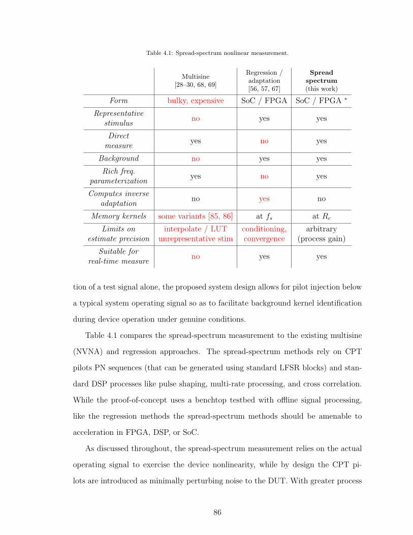
Table 4.1: Spread-spectrum nonlinear measurement.
Multisine[28–30, 68, 69]
Regression /adaptation[56, 57, 67]
Spreadspectrum(this work)
Form bulky, expensive SoC / FPGA SoC / FPGA ∗
Representativestimulus
no yes yes
Directmeasure
yes no yes
Background no yes yes
Rich freq.parameterization
yes no yes
Computes inverseadaptation
no yes no
Memory kernels some variants [85, 86] at fs at Rc
Limits onestimate precision
interpolate / LUTunrepresentative stim
conditioning,convergence
arbitrary(process gain)
Suitable forreal-time measure
no yes yes
tion of a test signal alone, the proposed system design allows for pilot injection below
a typical system operating signal so as to facilitate background kernel identification
during device operation under genuine conditions.
Table 4.1 compares the spread-spectrum measurement to the existing multisine
(NVNA) and regression approaches. The spread-spectrum methods rely on CPT
pilots PN sequences (that can be generated using standard LFSR blocks) and stan-
dard DSP processes like pulse shaping, multi-rate processing, and cross correlation.
While the proof-of-concept uses a benchtop testbed with offline signal processing,
like the regression methods the spread-spectrum methods should be amenable to
acceleration in FPGA, DSP, or SoC.
As discussed throughout, the spread-spectrum measurement relies on the actual
operating signal to exercise the device nonlinearity, while by design the CPT pi-
lots are introduced as minimally perturbing noise to the DUT. With greater process
86

gain, the CPT pilot power can be reduced even further (and the pilot margin cor-
respondingly increased). In contrast to the multisine approaches, this provides a
way for the spread-spectrum method to measure the nonlinearity subject to actual
(representative) stimulus.
In the spread-spectrum method the correlation for a given distortion component
is the coefficient measurement. In the multisine approach, the particular distortion
component magnitude and angle (like IMD3 for a two-tone analysis) is the coefficient
measurement. We refer to these as ‘direct’ measurements. In comparison to the
regression methods, these ‘direct’ measures avoid inference and matrix inversion on
stimulus and response data, and thus avoid the estimation limitations arising from
collinearity and poor conditioning.
Because the spread-spectrum correlation method avoids inverting a poorly-conditioned
matrix, the nonlinear coefficient estimate precision can be increased with process
gain. This avoids the conditioning problem that limits coefficient estimates in re-
gression approaches. Note that this measurement result is distinct from the matrix
inversion that may be needed to identify the nonlinear transfer inverse for predistor-
tion, which can still involve conditioning problems. And because the measurement
is made over code intervals on the actual operating signal, the spread-spectrum
method avoids the need to interpolate among benchtop measurements memorialized
in a lookup table.
The spread-spectrum measurement approximates the rich frequency parameter-
ization from a multisine approach. This provides a richer sampling of the nonlinear
transfer in multidimensional frequency space than the regression approaches, which
are designed to operate on the full bandwidth input and output stimulus response.
The spread-spectrum method also provides a straightforward way to estimate
coefficients memory coefficients on a channelized basis. The memory resolution in
the spread-spectrum approach is the chip rate, as compared to the sample rate for the
87

regression approaches. For long-term memory with time constants on the order of µs,
however, chip rates of 1 MHz or more should provide sufficient memory resolution.
Depending on the implementation, the spread-spectrum measurement may be
suitable for real-time nonlinear coefficient measurements. In this context ‘real-time’
means making measurements on the in situ DUT with temporal resolution of the
code dwell. This temporal resolution is decreasing in code length (process gain) but
increasing in chip rate (channel bandwidth).
4.2 Future directions for this research
This novel nonlinear measurement modality could provide a foundation for an active
research program, and/or form the basis of a commercial product or functionality.
Some possible directions for future research are summarized below.
4.2.1 Acceleration in FPGA, DSP, SoC, or ASIC
The approach is demonstrated using benchtop components, high speed 16-bit data
capture, and offline Matlab processing. A logical extension suitable for commercial-
ization would move the test signal generation, combination with the in situ operating
signal, sampling, and correlation in the RAKE architecture to a FPGA, DSP, SoC,
or ASIC. For example, the analog components could be provided by something like
the Analog Devices AD9361 transceiver or its successor parts, and the processing
done in a XilinX Zynq Ultrascale or comparable system on chip (SoC). This would
provide a step towards a real-time system measurement, although even in situ mea-
surement with processing lag would have value compared to cell tower base stations
that now use fixed lookup tables to develop linearizing predistortion.
88

4.2.2 Extend measurement parameters
There are several ways to further investigate the methodology by extending system
parameters and stimuli beyond those used in this work.
The demonstration shows Volterra kernel extraction using duobinary PN m-
sequences with primitive polynomials having order r = 20 for process gain ∼ 60
dB. In order to measure nonlinearity with a 20 dB pilot margin, future work should
investigate measurements using even longer codes and higher process gain, such as ∼
75 dB with primitive polynomials on order r = 25, or higher. Acceleration in FPGA
or SoC might aid this demonstration, with local test signal generation eliminating
an AWG memory requirement for test signal playback, and provided that system
integration reduces the insertion and path loss shown in the demonstration testbed
used in this work.
Future work should evaluate the Volterra kernel measurement with in situ oper-
ating signals (whether LTE or otherwise) rather than the discrete cyclical baseband
bandlimited Gaussian white noise model used in this work.
Further investigations can also characterize the measurement behavior with re-
spect to variations in chip rate and sampling channel bandwidth at different modu-
lating frequencies.
We have developed the spread-spectrum measurement for third-order distortion.
This covers a wide range of nonlinear device applications, but not all. In principle
the methodology extends to higher-order distortion terms, although this complicates
the code design requirements and correlated noise analysis. Further research into
code design and correlation measuring higher-order distortion is warranted.
89

4.2.3 Measure the distortion kernels for spectral broadening
This work limits kernel measurement to in-band distortion terms in order to evaluate
the distortion phase by reference to the CPT pilot in the linear testbed response.
Future work should investigate techniques to establish the distortion phase in the
spectrally-broadened regions, so as to characterize these additional distortion terms.
A related investigation can consider the effect on nonlinear measurement by vary-
ing the pilot frequency division. In this work five pilots are used in 2 MHz channels
to span a 10 MHz operating signal. There is no a priori reason, however, to require
that the pilots contiguously span the operating signal. Given the nonlinear order, the
pilot offset frequencies determine the frequencies of the resulting coded distortions
that can be measured. It may be more efficient to measure nonlinear kernels with
sparser, or noncontiguous, pilot placement.
4.2.4 Device characterization
The methodology can further be used to investigate nonlinearity for a panel of de-
vices with variations in operating frequencies, temperatures, and operating signal
bandwidths. In principle this approach can be refined to define a standard device
nonlinearity characterization with greater detail than reference to IP3.
4.2.5 Ultrawideband systems
This work shows nonlinear measurement for 10 MHz signals at 2 GHz. Given in-
dustry interest in ultrawideband systems (at 30 GHz and higher), and 5G plans
to aggregate 20 MHz signals to bandwidths of 100 MHz or more, future research
should investigate the spread-spectrum methodology for characterizing nonlinearity
in ultrawideband devices or systems.
90

4.2.6 Novel system design
We show the spread-spectrum measurement using complex pseudoternary pilots de-
fined over GF(2). The rich literature in spread-spectrum signal design and algebraic
coding theory could provide insight on other pilot designs useful in this nonlinear
measurement, subject to the constraints and considerations set forth in Chapter 3.
4.2.7 Calibration
Different efforts at calibrating the nonlinear measurement in this work have con-
sumed inordinate time. Several microwave circuits were tried. Comparing measure-
ments on a shunt Schottky diode on a 50Ω stripline to two-tone ADS simulations pro-
vide marginally acceptable calibration so as to report kernel magnitudes in absolute
( 1V 2 ) terms. Future research should focus on improving and defining a standardized
nonlinear calibration methodology.
4.2.8 Predistortion
Future work includes applying the nonlinear parameters measured using the spread-
spectrum methodology to demonstrate digital predistortion.
4.2.9 Novel memory polynomials
Note that the spread-spectrum methodology develops memory polynomials on a
channel basis, that is, it provides a distinct behavioral model for each in-band chan-
nel. This contrasts with the canonical memory polynomial models, which provide
representations across the entire first-zone distorted signal bandwidth. In addition,
we have explicitly shown the spread-spectrum methodology only for third-order dis-
tortions, whereas the memory polynomial representations often probe the nonlin-
earity to higher-order distortions. Extending the spread-spectrum measurement to
91

higher-order nonlinearity, and combining the channel-specific nonlinear parameters
in a representation for the full in-band (or spectrally-broadened) signal, remain topics
for future investigation.
4.2.10 Optical systems
Although this work is developed by reference to nonlinear PA in a transmit ar-
chitecture, several electrically-driven optical devices (lasers, phase modulators) in
integrated microwave photonics can also benefit from linearization schemes. As a
result, it may be worth investigating how the spread-spectrum nonlinear measure-
ment modality could apply to measure, then mitigate, nonlinear responses in these
optical devices.
4.2.11 Nonlinear theory
The spread-spectrum methodology is shown with rich sampling for the nonlinear
transfer in three-dimensional frequency space. Further work can be done to unify
the theoretical consideration of measurements on a channel base with the kernel
estimates provided by the common regression or adaptive techniques to identify the
nonlinear inverse for predistortion.
92

BIBLIOGRAPHY
[1] W. J. Rugh, Nonlinear System Theory: The Volterra/Wiener Approach. TheJohns Hopkins University Press, 1981.
[2] E. Heredia and G. Arce, “Piecewise Volterra filters based on the threshold de-composition operator,” in 1996 IEEE International Conference on Acoustics,Speech, and Signal Processing Conference Proceedings, vol. 3. IEEE, 1996, pp.1593–1596.
[3] P. Singerl and G. Kubin, “Constructing memory-polynomial models fromfrequency-dependent am/am and am/pm measurements,” in 2007 50th Mid-west Symposium on Circuits and Systems, Aug 2007, pp. 321–324.
[4] S. Benedetto and E. Biglieri, Principles of Digital Transmission: With WirelessApplications. New York: Kluwer Academic, 1999.
[5] S. Boyd and L. Chua, “Fading memory and the problem of approximating non-linear operators with Volterra series,” IEEE Transactions on Circuits and Sys-tems, vol. 32, no. 11, pp. 1150–1161, 1985.
[6] J. Bussgang, L. Ehrman, and J. Graham, “Analysis of nonlinear systems withmultiple inputs,” Proceedings of the IEEE, vol. 62, no. 8, 1974.
[7] M. Schetzen, “Nonlinear System Modeling Based on the Wiener Theory,” Pro-ceedings of the IEEE, vol. 69, no. 12, pp. 1557–1573, 1981.
[8] C. M. Cheng, Z. K. Peng, W. M. Zhang, and G. Meng, “Wavelet basis expansion-based Volterra kernel function identification through multilevel excitations,”Nonlinear Dynamics, vol. 76, no. 2, pp. 985–999, 2014.
[9] S. Benedetto, E. Biglieri, and R. Daffara, “Modeling and Performance Evalu-ation of Nonlinear Satellite Links-A Volterra Series Approach,” IEEE Trans-actions on Aerospace and Electronic Systems, vol. AES-15, no. 4, pp. 494–507,1979.
[10] P. Singerl, A. Agrawal, A. Garg, Neelabh, G. Kubin, and H. Eul, “ComplexBaseband Predistorters for Nonlinear Wideband RF Power Amplifiers,” in 200649th IEEE International Midwest Symposium on Circuits and Systems, vol. 2,no. 1, 2006, pp. 675–678.
93

[11] P. Singerl, “Complex Baseband Modeling and Digital Predistortion for Wide-band RF Power Amplifiers,” Ph.D. dissertation, Graz University of Technology,Austria, 2006.
[12] P. M. S. Burt and J. H. de Morais Goulart, “Efficient Computation of BilinearApproximations and Volterra Models of Nonlinear Systems,” IEEE Transactionson Signal Processing, vol. PP, no. 99, pp. 1–1, 2017.
[13] T. Wang and T. J. Brazil, “Volterra-mapping-based behavioral modeling ofnonlinear circuits and systems for high frequencies,” IEEE Transactions onMicrowave Theory and Techniques, vol. 51, no. 5, pp. 1433–1440, 2003.
[14] M. Isaksson, D. Wisell, and D. Ronnow, “A comparative analysis of behavioralmodels for RF power amplifiers,” IEEE Transactions on Microwave Theory andTechniques, vol. 54, no. 1, pp. 348–359, 2006.
[15] J. C. Pedro and S. A. Maas, “A Comparative Overview of Microwave and Wire-less Power Amplifier Behavioral Modeling Approaches,” IEEE Transactions onMicrowave Theory and Techniques, vol. 53, no. 4, pp. 1150–1163, 2005.
[16] M. Zeller, L. A. Azpicueta-Ruiz, J. Arenas-Garcıa, and W. Kellermann, “Adap-tive Volterra filters with evolutionary quadratic kernels using a combinationscheme for memory control,” IEEE Transactions on Signal Processing, vol. 59,no. 4, pp. 1449–1464, 2011.
[17] T. Ogunfunmi, Adaptive Nonlinear System Identification, ser. Signals And Com-munication Technology. Boston, MA: Springer US, 2007.
[18] G. Valenza, L. Citi, E. P. Scilingo, and R. Barbieri, “Point-process nonlinearmodels with Laguerre and Volterra expansions: Instantaneous assessment ofheartbeat dynamics,” IEEE Transactions on Signal Processing, vol. 61, no. 11,pp. 2914–2926, 2013.
[19] P. Wambacq and W. Sansen, Distortion Analysis of Analog Integrated Circuits.Kluwer, 1998.
[20] B. Razavi, RF Microelectronics, 2nd ed. Pearson Education, Inc., 2012.
[21] N. Wiener, “Response of a Non-Linear Device to Noise,” Massachusetts Insti-tute of Technology, Radiation Laboratory Report No. 165, Cambridge, Mas-sachusetts, Tech. Rep., 1942.
[22] E. Bedrosian and S. O. Rice, “The Output Properties of Volterra Systems (Non-linear Systems with Memory) Driven by Harmonic and Gaussian Inputs,” Pro-ceedings of the IEEE, vol. 59, no. 12, pp. 1688–1707, 1971.
[23] G. B. Giannakis and E. Serpedin, “A bibliography on nonlinear system identi-fication,” Signal Processing, vol. 81, no. 3, pp. 533–580, 2001.
[24] G. Palm and T. Poggio, “The Volterra Representation and the Wiener Expan-sion: Validity and Pitfalls,” SIAM Journal on Applied Mathematics, vol. 33,no. 2, pp. 195–216, 1977.
94

[25] L. Chua and C. Ng, “Frequency-domain analysis of nonlinear systems: formu-lation of transfer functions,” IEE Journal on Electronic Circuits and Systems,vol. 3, no. 6, p. 257, 1979.
[26] ——, “Frequency domain analysis of nonlinear systems: general theory,” IEEJournal on Electronic Circuits and Systems, vol. 3, no. 4, pp. 165–185, 1979.
[27] P. Wambacq, G. G. Gielen, P. R. Kinget, and W. Sansen, “High-FrequencyDistortion Analysis of Analog Integrated Circuits,” IEEE Transactions on Cir-cuits and Systems—II: Analog and DIgital Signal Processing, vol. 46, no. 3, pp.335–345, 1999.
[28] D. E. Root, J. Verspecht, D. Sharrit, J. Wood, and A. Cognata, “Broad-bandPoly-Harmonic Distortion (PHD) behavioral models from fast automated sim-ulations and large-signal vectorial network measurements,” IEEE Transactionson Microwave Theory and Techniques, vol. 53, no. 11, pp. 3656–3664, 2005.
[29] D. E. Root, J. Xu, J. Horn, M. Iwamoto, and G. Simpson, “Device modelingwith NVNAs and X-parameters,” in 2010 Workshop on Integrated NonlinearMicrowave and Millimetre-Wave Circuits, INMMiC 2010 - Conference Proceed-ings, 2010, pp. 12–15.
[30] P. Roblin, Nonlinear RF Circuits and Nonlinear Vector Network Analyzers:Interactive Measurement and Design Techniques. Cambridge, UK: CambridgeUniversity Press, 2011.
[31] N. Wiener, Non Linear Problems in Random Theory. Technology Press of theMassachusetts Institute of Technology and John Wiley & Sons, Inc., 1958.
[32] Y. W. Lee and M. Schetzen, “Measurement of the Wiener Kernels of a Non-linear System by Cross-correlation,” International Journal of Control, vol. 2,no. 3, pp. 237–254, 1965.
[33] R. Simpson and H. Power, “Correlation Techniques for the Identification ofNon-Linear Systems,” Measurement and Control, vol. 5, no. 8, pp. 316–321,1972.
[34] A. G. Bose, “A Theory of Nonlinear Systems,” Ph.D. dissertation, Mas-sachusetts Institute of Technology, 1956.
[35] E. P. Gyftopoulos and R. J. Hooper, “Signals for Transfer Function Measure-ments in Nonlinear Systems,” in Proc. of Conf. on Noise Analysis in NuclearSystems, no. CONF-332-11. U.S. Atomic Energy Commission, 1964, pp. 335–345.
[36] S. Orcioni, “Improving the approximation ability of volterra series identifiedwith a cross-correlation method,” Nonlinear Dynamics, vol. 78, no. 4, pp. 2861–2869, 2014.
[37] G. Favier, A. Y. Kibangou, and T. Bouilloc, “Nonlinear system modelingand identification using Volterra-PARAFAC models,” International Journal ofAdaptive Control and Signal Processing, vol. 26, no. 1, pp. 30–53, jan 2012.
95

[38] M. O. Franz and B. Scholkopf, “A Unifying View of Wiener and Volterra Theoryand Polynomial Kernel Regression,” Neural Computation, vol. 18, no. 12, pp.3097–3118, 2006.
[39] V. Z. Marmarelis, “Modeling methodology for nonlinear physiological systems.”Annals of Biomedical Engineering, vol. 25, no. 2, pp. 239–251, 1997.
[40] K. Godfrey, “Three-Level mSequences,” Electronics Letters, vol. 2, no. 7, pp.241–243, 1966.
[41] H. Barker and S. Obidegwu, “Combined crosscorrelation method for the mea-surement of 2nd-order Volterra kernels,” Proceedings of the Institution of Elec-trical Engineers, vol. 120, no. 1, p. 114, 1973.
[42] H. A. Barker and R. W. Davy, “Measurement of second-order Volterra kernelsusing pseudorandom ternary signals,” International Journal of Control, vol. 27,no. 2, pp. 277–291, 1978.
[43] ——, “2nd - order Volterra kernel measurement using pseudorandom ternarysignals and discrete Fourier transforms,” Proceedings of IEE, vol. 126, no. 5, pp.457–460, 1979.
[44] H. A. Barker, A. H. Tan, and K. R. Godfrey, “Optimal levels of perturbationsignals for nonlinear system identification,” IEEE Transactions on AutomaticControl, vol. 49, no. 8, pp. 1404–1407, 2004.
[45] K. R. Godfrey, A. H. Tan, H. A. Barker, and B. Chong, “A survey of readily ac-cessible perturbation signals for system identification in the frequency domain,”Control Engineering Practice, vol. 13, no. 11, pp. 1391–1402, 2005.
[46] A. H. Tan and K. R. Godfrey, “A guide to the design and selection of perturba-tion signals,” in Proceedings of the IEEE Conference on Decision and Control,2009, pp. 464–469.
[47] S. Boyd, Y. Tang, and L. Chua, “Measuring Volterra kernels,” IEEE Transac-tions on Circuits and Systems, vol. 30, no. 8, pp. 571–577, 1983.
[48] P. Lavrador, T. Cunha, P. Cabral, and J. Pedro, “The Linearity-EfficiencyCompromise,” IEEE Microwave Magazine, vol. 11, no. 5, pp. 44–58, aug 2010.
[49] G. Zhou, “Analysis of spectral regrowth of weakly nonlinear power amplifiers,”IEEE Communications Letters, vol. 4, no. 11, pp. 357–359, 2000.
[50] K. G. Gard, L. E. Larson, and M. B. Steer, “The impact of RF front-end char-acteristics on the spectral regrowth of communications signals,” IEEE Trans-actions on Microwave Theory and Techniques, vol. 53, no. 6, pp. 2179–2185,2005.
[51] Z. El-Khatib, L. MacEachern, and S. A. Mahmoud, Distributed CMOS Bidirec-tional Amplifiers. New York, NY: Springer New York, 2012.
[52] T. Nesimoglu, RF and Microwave Amplifier Linearization for Wireless Com-munication: Harmonic Injections and Polynomial Predistortion. Saarbrucken,Germany: VDM Verlag, 2011.
96
[53] S. Maas, “Linearity and Dynamic Range of Carbon Nanotube Field-Effect Tran-sistors,” in 2017 IEEE MTT S International Microwave Symposium (IMS),2017, pp. 1–4.
[54] DARPA Microsystems Technology Office BAA No. HR001117S0024, “DynamicRange-enhanced Electronics and Materials (DREaM),” pp. 1–45, March 2017.
[55] H. Jiang and P. Wilford, “Digital Predistortion for Power Amplifiers UsingSeparable Functions,” IEEE Transactions on Signal Processing, vol. 58, no. 8,pp. 4121–4130, 2010.
[56] D. R. Morgan, Z. MA, J. Kim, M. G. Zierdt, and J. Pastalan, “A GeneralizedMemory Polynomial Model for Digital Predistortion of RF Power Amplifiers,”IEEE Transactions on Signal Processing, vol. 54, no. 10, pp. 3852–3860, 2006.
[57] A. Zhu, P. J. Draxler, J. J. Yan, T. J. Brazil, D. F. Kimball, and P. M. As-beck, “Open Loop Digital Predistorter for RF Power Amplifiers Using DynamicDeviation Reduction-Based Volterra Series,” IEEE Transactions on MicrowaveTheory and Techniques, vol. 56, no. 7, pp. 1–10, 2008.
[58] A. Zhu, M. Wren, and T. Brazil, “An efficient Volterra-based behavioral modelfor wideband RF power amplifiers,” in IEEE MTT-S International MicrowaveSymposium Digest, 2003, vol. 2, 2003, pp. 3–6.
[59] J. Wood and D. E. Root, Eds., Fundamentals of Nonlinear Behavioral Modelingfor RF and Microwave Design. Norwood, MA: Artech House, 2005.
[60] N. B. de Carvalho and J. C. Pedro, “A comprehensive explanation of distortionsideband asymmetries,” IEEE Transactions on Microwave Theory and Tech-niques, vol. 50, no. 9, pp. 2090–2101, 2002.
[61] D. D. Silveira, P. L. Gilabert, P. M. Lavrador, J. C. Pedro, M. Gadringer,G. Montoro, E. Bertran, and G. Magerl, “Improvements and Analysis of Non-linear Parallel Behavioral Models,” International Journal of RF and MicrowaveComputer-Aided Engineering, vol. 19, no. 5, pp. 615–626, 2009.
[62] S. Chen, W. Panton, and R. Gilmore, “Effects on nonlinear distortion onCDMA communication systems,” IEEE Transactions on Microwave Theoryand Tecniques, vol. 44, no. 12, pp. 2743–2750, 1996.
[63] S. C. Cripps, RF Power Amplifiers for Wireless Communications, 2nd ed. Nor-wood, MA: Artech House, 2006.
[64] D. Wisell, “A baseband time domain measurement system for dynamic charac-terization of power amplifiers with high dynamic range over large bandwidths,”in Proceedings of the 20th IEEE Instrumentation and Measurement TechnologyConference, vol. 2, 2003, pp. 1177–1180.
[65] P. Cabral, J. Pedro, and N. Carvalho, “Dynamic AM-AM and AM-PM Be-havior in Microwave PA Circuits,” in 2005 Asia-Pacific Microwave ConferenceProceedings, vol. 4. IEEE, 2005, pp. 1–4.
97

[66] L. C. Nunes, P. M. Cabral, and J. C. Pedro, “A physical model of power ampli-fiers AM/AM and AM/PM distortions and their internal relationship,” in 2013IEEE MTT-S International Microwave Symposium Digest (MTT). IEEE, jun2013, pp. 1–4.
[67] J. Kim and K. Konstantinou, “Digital predistortion of wideband signals basedon power amplifier model with memory,” Electronics Letters, vol. 37, no. 23,pp. 1417–18, 2001.
[68] P. Roblin, Y. S. Ko, C. K. Yang, I. Suh, and S. J. Doo, “NVNA Techniquesfor Pulsed RF Measurements,” IEEE Microwave Magazine, vol. 12, no. 2, pp.65–76, 2011.
[69] G. Simpson, J. Horn, D. Gunyan, and D. E. Root, “Load-Pull + NVNA =Enhanced X-Parameters for PA Designs with High Mismatch and Technology-Independent Large-Signal Device Models,” in 2008 72nd ARFTG MicrowaveMeasurement Symposium, ARFTG 2008, 2008, pp. 88–91.
[70] D. Ronnow, D. Wisell, and M. Isaksson, “Three-tone characterization of non-linear memory effects in radio-frequency power amplifiers,” IEEE Transactionson Instrumentation and Measurement, vol. 56, no. 6, pp. 2646–2657, 2007.
[71] J. Vuolevi, T. Rahkonen, and J. Manninen, “Measurement technique for char-acterizing memory effects in RF power amplifiers,” IEEE Transactions on Mi-crowave Theory and Techniques, vol. 49, no. 8, pp. 1383–1389, 2001.
[72] C. P. Silva, C. J. Clark, A. A. Moulthrop, and M. S. Muha, “Survey of char-acterization techniques for nonlinear communication components and systems,”in IEEE Aerospace Conference Proceedings, 2005, pp. 1–25.
[73] C. P. Silva, “Time-domain measurement and modeling techniques for widebandcommunication components and systems,” International Journal of RF and Mi-crowave Computer-Aided Engineering, vol. 13, no. 1, pp. 5–31, 2003.
[74] W. Bosch and G. Gatti, “Measurement and simulation of memory effects inpredistortion linearizers,” IEEE Transactions on Microwave Theory and Tech-niques, vol. 37, no. 12, pp. 1885–1890, 1989.
[75] B. Schubert, J. Liszewski, and W. Keusgen, “Identification of the Volterra ker-nels of nonlinear power amplifiers,” in IEEE International Conference on Com-munications, Circuits and Systems (ICCCAS’09), 2009, pp. 767–771.
[76] A. Zhu and T. Brazil, “Behavioral modeling of RF power amplifiers based onpruned Volterra series,” IEEE Microwave and Wireless Components Letters,vol. 14, no. 12, pp. 563–565, 2004.
[77] P. Jaraut, G. C. Tripathi, M. Rawat, and P. Roblin, “Independent componentanalysis for multi-carrier transmission for 4G/5G power amplifiers,” in 201789th ARFTG Microwave Measurement Conference (ARFTG), June 2017, pp.1–4.
98

[78] E. Ngoya and S. Mons, “Progress for behavioral challenges: A summary oftime-domain behavioral modeling of RF and microwave subsystems,” IEEE Mi-crowave Magazine, vol. 15, no. 6, pp. 91–105, 2014.
[79] D. A. Belsley, E. Kuh, and R. E. Welsch, Regression Diagnostics: IdentifyingInfluential Data And Sources of Collinearity. John Wiley & Sons, 1980.
[80] M. Li, I. Galton, L. Larson, and P. Asbeck, “Correlation techniques for esti-mation of amplifier nonlinearity,” in Proceedings of the 2004 IEEE Radio andWireless Conference, 2004, pp. 179–182.
[81] ——, “Nonlinearity estimation and spectral regrowth prediction of power am-plifiers using correlation techniques,” in IEEE Annual Conference Wireless andMicrowave Technology, 2005, pp. 170–173.
[82] A. Panigada and I. Galton, “Digital background correction of harmonic distor-tion in pipelined adcs,” IEEE Transactions on Circuits and Systems I: RegularPapers, vol. 53, no. 9, pp. 1885–1895, Sept 2006.
[83] G. Ballantyne, “Code domain analysis of nonlinear links,” Electronics Letters,vol. 44, no. 21, pp. 1–2, 2008.
[84] A. R. Wichman and L. E. Larson, “Background Measurement of RF Sys-tem Nonlinearity Using Spread-Spectrum Methods,” in 2017 90th ARFTGMicrowave Measurement Conference (ARFTG), November 2017, pp. 1–4, (inpress).
[85] J. Verspecht, J. Horn, and D. E. Root, “A Simplified Extension of X-parametersto Describe Memory Effects for Wideband Modulated Signals,” in 75th ARFTGConf. Rec., 2010, pp. 1–6.
[86] J. Verspecht, T. Nielson, and D. Root, “Digital predistortion method basedon dynamic X-parameters,” in Novel 5G Applications of Nonlinear Vector Net-work Analyzer for Broadband Modulation and Millimeter Wave CharacterizationWorkshop, IMS 2017. Honolulu: Int’l Microwave Symp., 2017.
[87] R. Pickholtz, D. Schilling, and L. Milstein, “Theory of Spread-SpectrumCommunications–A Tutorial,” IEEE Transactions on Communications, vol. 30,no. 5, pp. 855–884, 1982.
[88] D. V. Sarwate and M. B. Pursley, “Crosscorrelation properties of pseudorandomand related sequences,” Proceedings of the IEEE, vol. 68, no. 593, pp. 170–182,1980.
[89] B. Sklar, Digital Communications Fundamentals and Applications. EnglewoodCliffs, NJ: Prentice-Hall, 1988.
[90] D. Torrieri, Principles of Spread-Spectrum Communication Systems. Springer,2005.
[91] Solomon W. Golomb and Guang Gong, Signal Design for Good Correlation:For Wireless Communication, Cryptography, and Radar. New York, NY: Cam-bridge University Press, 2005.
99

[92] R. Enomoto, H. Habuchi, and K. Hashiura, “Performance of DS/SS SystemUsing Pseudo-Ternary M-Sequences,” IEICE Transactions on Fundamentals ofElectronics, Communications and Computer Sciences, no. 11, pp. 2299–2306,2010.
[93] J. G. Proakis and M. Salehi, Digital Communications, 5th ed. McGraw-Hill,Inc., 2008.
[94] R. W. Boyd, Nonlinear Optics, 3rd ed. Academic Press, 2008.
[95] J. Verspecht and D. E. Root, “Polyharmonic distortion modeling,” IEEE Mi-crowave Magazine, vol. 7, no. 3, pp. 44–57, 2006.
[96] J. Pedro, N. Carvalho, and P. Lavrador, “Modeling nonlinear behavior of band-pass memoryless and dynamic systems,” in IEEE MTT-S International Mi-crowave Symposium Digest, 2003, vol. 3, 2003, pp. 2133–2136.
[97] J. Graham and L. Ehrman, “Nonlinear system modeling and analysis with ap-plications to communications receivers,” Rome Air Development Center, Tech.Rep. June, 1973.
100

APPENDIX A
Definition of Terms
List of Abbreviations
IM3 relative third-order intermodulation
m-sequence maximal length PN sequence
ACPR adjacent channel power ratio
ADC analog to digital converter
ADS Keysight Advanced Design System
AGC automatic gain control
AM amplitude modulation
AM/AM, AM/PM nonlinear amplitude (AM/AM) and phase (AM/PM) modula-
tion with signal amplitude
ASIC application specific integrated circuit
101

AWG arbitrary wave generator
AWGN additive white Gaussian noise
BPSK binary phase shift key
CDMA code dividion multiple access
CPT complex pseudoternary
CW continuous wave
DAC digital to analog converter
DSSS direct sequence spread-spectrum
DUT device under test
FPGA field programmable gate array
IC intermodulation code
IIP3 input-referred third-order intermodulation point
IMD3 cubic intermodulation distortion
IP3 third-order intercept point
IP3 third-order intermodulation product
IS-95 TIA/EIA IS-95 Mobile Station-Base Station Compatibility Standard for Dual-
Mode Wideband Spectrum Cellular Systems
LFSR linear feedback shift register
LO local oscillator
LTI linear time invariant
102

LUT lookup table
NVNA nonlinear vector network analyzer
ODFM orthogonal frequency division multiplexing
OIP3 output-referred third-order intermodulation point
PA power amplifier
PAE power added efficiency ηPAE = Pout−Pin
Pdc
PAPR peak to average power ratio, same as crest factor in dB
PG process gain
PLL phase locked loop
PM pilot margin
PN pseudorandom noise
PT pseudoternary
RF radio frequency
SCN spread code noise
SINR signal to interference and noise ratio
SMD3 cubic self-modulation distortion
SoC system on chip
TPD3 cubic triple product distortion
XMD3 cubic cross-modulation distortion
XOR exclusive OR
103

List of Symbols
APM reference PN amplitude for given PM with AWG full scale range ± 1V
ˆhqij lowpass equivalent Volterra kernel estimate for order i, position j, due to
pilots at q
ωB baseband operating signal radial bandwidth
ωi baseband offset radial frequency for channel i
ωLO LO radial frequency
Ψi(t) analytic pilot in offset channel i
cqi = T pq,ic duobinary maximal length PN sequence in channel i with phase q (pq,i)
η(t) baseband operating signal
s(t) lowpass equivalent composite pilots and operating signal
x(t) lowpass-equivalent composite FDM pilots
xi(t) lowpass-equivalent pilot in channel i
y(t) DUT distortion envelope
yijk3 (n) first-zone lowpass-equivalent discrete cubic distortion due to pilots at i, j, k
Ai pilot PN amplitude in channel i
D dwell (code interval N · Tc)
F [·] first-zone filter
fB DAC output bandwidth
fs sample rate (ADC unless otherwise noted)
104

fLO local oscillator frequency
G[·] nonlinear operator
H[·] first-zone nonlinear operator
L testbed conversion and path loss from AWG to DUT input
N code length (unless otherwise noted)
N0 lowpass equivalent operating signal s(t) power in mW at DAC (AWG) output
across ±fB
r primitive polynomial order
Rc chip rate
T (·) cyclical left shift operator
Tc chip interval
Xq DUT output operating signal power in dBm at channel q
y(t) DUT output
z correlator output
GF(2) second-order Galois field
Tx DAC (AWG) signal power relative to ±1V scale
105
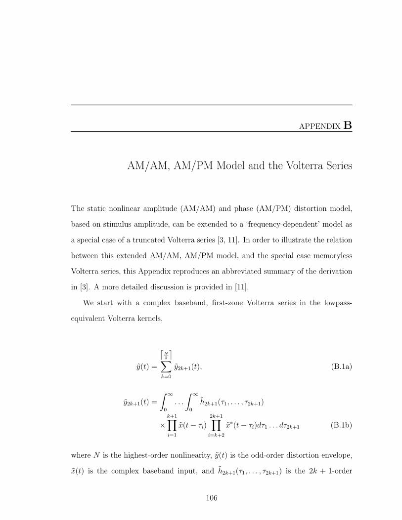
APPENDIX B
AM/AM, AM/PM Model and the Volterra Series
The static nonlinear amplitude (AM/AM) and phase (AM/PM) distortion model,
based on stimulus amplitude, can be extended to a ‘frequency-dependent’ model as
a special case of a truncated Volterra series [3, 11]. In order to illustrate the relation
between this extended AM/AM, AM/PM model, and the special case memoryless
Volterra series, this Appendix reproduces an abbreviated summary of the derivation
in [3]. A more detailed discussion is provided in [11].
We start with a complex baseband, first-zone Volterra series in the lowpass-
equivalent Volterra kernels,
y(t) =
⌈N2
⌉∑k=0
y2k+1(t), (B.1a)
y2k+1(t) =
∫ ∞
0
. . .
∫ ∞
0
h2k+1(τ1, . . . , τ2k+1)
×k+1∏i=1
x(t− τi)2k+1∏i=k+2
x∗(t− τi)dτ1 . . . dτ2k+1 (B.1b)
where N is the highest-order nonlinearity, y(t) is the odd-order distortion envelope,
x(t) is the complex baseband input, and h2k+1(τ1, . . . , τ2k+1) is the 2k + 1-order
106

lowpass-equivalent Volterra kernel.
B.1 Memoryless Volterra kernel
We restrict the representation to a “memoryless” system by constraining the off-
diagonal Volterra kernels to be zero, h2k+1(τ1, . . . , τ2k+1) ≡ 0 unless τ1 = τ2 = . . . =
τ2k+1.
A stationary linear system with kernel h(t) has system transfer function
H(s) =
∫ ∞
0
h(t)exp(−st)dt. (B.2)
For one-sided input signal u(t),
y(t) =
∫ ∞
−∞h(τ)u(t− τ)dτ (B.3)
=
∫ ∞
0
h(τ)u(t− τ)dτ
which reduces to
Y (s) = H(s)U(s). (B.4)
For a degree-n homogenous system with one-sided inputs,
y(t) =
∫ ∞
−∞. . .
∫ ∞
−∞h(τ1, . . . , τn)u(t− τ1) . . . u(t− τn)dτ1 . . . dτn. (B.5)
The nth-order term in y(t) =∑N
n=1 yn(t) is
yn(t1, . . . , tn) =
∫ t1
0
. . .
∫ tn
0
h(τ1, . . . , τn) (B.6)
×u(t− τ1) . . . u(t− τn)dτ1 . . . dτn.
107

The multidimensional transform
Y (s1, . . . , sn) =
∫ ∞
0
. . .
∫ ∞
0
y(t1, . . . , tn)exp(−n∑
i=1
siti)dt1 . . . dtn. (B.7)
Using
y(t) = yn(t1, . . . , tn)∣∣∣t1=...=tn=t
= yn(t, . . . , t), (B.8)
write
L[y(t1, . . . , tn)
]∣∣∣t1=...=tn=t
= (B.9)∫ ∞
0
. . .
∫ ∞
0
y(t1, . . . , tn)exp
(−
n∑i=1
siti
)dt1 . . . dtn
=
∫ ∞
0
y(t)exp
(−
(n∑
i=1
si
)t
)dt
= Y (s1 + s2 + . . .+ sn).
So this implies that L[hn(t1, . . . , tn)
]at t = t1 = . . . = tn is Hn(s1+ s2+ . . .+ sn), or
L[yn(t1, . . . , tn)
]∣∣∣t1=...=tn=t
= Y (s1 + s2 + . . .+ sn) (B.10)
= Hn(s1 + s2 + . . .+ sn)X(s1) . . . X(sn).
B.2 Relation to AM/AM, AM/PM model
Applying this restriction to the higher-order Volterra kernels from (B.1b) and sub-
stituting in (B.1a) simplifies the complex baseband Volterra series to
y(t) =
⌈N2
⌉∑k=0
∫ ∞
0
h2k+1(τ)x(t− τ)∣∣x(t− τ)
∣∣2kdτ. (B.11)
108

Now apply a complex baseband two-tone signal x(t) = acos(ωwt + ϕ) in (B.11),
so that the two-tone response is
y(t) =
⌈N2
⌉∑k=0
(a2
)2k+1 ∫ ∞
0
h2k+1(τ)
[exp (jζ) + exp (−jζ)
]2k+1
dτ, (B.12)
with ζ = ωm(t− τ) + ϕ.
Expanding the bracketed quantity in (B.12) and pulling the constant terms out-
side the integral,
y(t) =
⌈N2
⌉∑k=0
(a2
)2k+1 2k+1∑n=0
2k + 1
n
exp
j(2n− 2k − 1)ωmt
+(2n− 2k − 1)ϕ
(B.13)
×∫ ∞
0
h2k+1(τ)exp (−j(2n− 2k − 1)ωmτ)) dτ.
The first-zone components near angular fundamental ωm in (B.13) are selected
by requiring n = k + 1, representing the effect of applying a first-zone filter to the
two-tone response in (B.12) and (B.13). Then (B.13) reduces to
yf (t) = exp(jωmt+ ϕ)
[ ⌈N2
⌉∑k=0
(a2
)2k+1
2k + 1
k + 1
H2k+1(ωm)
](B.14)
where H2k+1(ωm) =∫∞−∞ h2k+1(τ)exp(−jωmτ)dτ , and yf (t) is the first-zone output
envelope.
From (B.14) we define the bracketed-quantity as a complex-valued function
v(a, ωm) =
⌈N2
⌉∑k=0
(a2
)2k+1
2k + 1
k + 1
H2k+1(ωm). (B.15)
109

Then we can express the first-zone, lowpass-equivalent output of the two-tone
stimulus in terms of (B.15) as
yf (t) =∣∣v(a, ωm)
∣∣exp(j (ωmt+ ϕ+ argv(a, ωm))
). (B.16)
This provides the desired relationship. (B.16) expresses the AM/AM, AM/PM
nonlinear representation in terms of a “memoryless” Volterra series, in a lowpass-
equivalent first-zone representation, with complex-valued Volterra kernels, through
the complex coefficient v(a, ωm). At the carrier ωm the magnitude∣∣v(a, ωm)
∣∣ rep-resents the AM/AM distortion response to the stimulus amplitude, and the angle
argv(a, ωm) represents the AM/PM distortion response to the stimulus.
110

APPENDIX C
Direct Sequence Spread-Spectrum
This appendix summarizes various results in direct sequence spread-spectrum rele-
vant to the nonlinear kernel measurement. The development follows [87, 89, 90].
C.1 Signal model
A transmitter sends a signaling waveform si(t), 0 ≤ t ≤ T ; 1 ≤ i ≤ M . In a
channel this combines with additive white Gaussian noise (AWGN) n(t) with two-
sided power spectral density η0/2 in WHz. A receiver detects r(t) = si(t) + n(t) over a
symbol interval [0, T ] [87].
Given a specific signal design, communication system performance is a function of
the energy per bit to noise spectral density [87]. An optimum detector with additive
white Gaussian noise (AWGN) is a bank of correlators [87], which are matched filters
over an integration (symbol interval) [89].
C.2 Processing gain
The spread-spectrum technique distributes a low-dimensional signal in high-dimensional
signal space [87, 89].
111

C.2.1 Signal
Take D orthogonal signals si(t), 1 ≤ i ≤ D in N -dimensional signal space, with
D < N . Each signal can be expanded on an orthonormal basis,
si(t) =N∑j=1
aijϕj(t), (C.1)
with aij = ⟨si(t), ϕj(t)⟩ and ⟨ϕj(t), ϕk(t)⟩ = δjk.
The orthonormal basis functions ϕj(t) span the N -dimensional signal space. The
coefficients aij (the ‘signaling coefficients’) are BPSK PN sequence chip j values
for signal i with alphabet ±a and Pr(a) = 12.
The energy is assumed equal in each signal waveform, with each signal having
average energy
Es = E[si(t)2] =
∫ T
o
s2i (t)dt =N∑j=1
a2ij. (C.2)
The spreading sequences are orthogonal in the sense that for each sequence the
coefficients are independently selected with zero mean and correlation aijaik =Es
Nδjk,
1 ≤ i ≤ D.
C.2.2 Jammer
A jammer is represented by expansion on the same basis functions,
J(t) =N∑k=1
Jkϕk(t) (C.3)
with total energy
EJ =
∫ T
o
J2(t)dt =N∑k=1
J2k . (C.4)
112

For analysis receiver noise is ignored and the received signal is
r(t) = si(t) + J(t). (C.5)
In the spread-spectrum nonlinear kernel measurement, the jammer J(t) is the desired
operating signal η(t).
C.2.3 Correlation
The received signal is correlated against possible transmitted signals (the known
spreading sequences),
r(t) = si(t) + J(t). (C.6)
The ith correlator output is
zi = ⟨r(t), si(t)⟩ (C.7)
=
∫ T
0
r(t)si(t)dt
=N∑k=1
(a2ik + Jkaik.
)
Then given si transmitted, assuming the jammer is independent of the spreading
sequence E(Jkaik) = 0, the correlation output signal energy is
E(zi|si) =N∑k=1
a2ik = Es. (C.8)
With D equiprobable transmitted signals,
E(zi) =Es
D. (C.9)
113

The correlation variance given ith signal transmission is
var(zi|si) =∑k,l
JkJlaikail (C.10)
=N∑k=1
J2ka
2ik
=Es
NEJ ,
var(zi) =Es
NDEJ . (C.11)
The signal-to-noise (jammer) ratio can be expressed as
SNR =E2(z)
var(z)(C.12)
=Es
EJ
(N
D
).
The ratio(ND
)is the process gain [87, 89]. In terms of the relative signal band-
widths, which have approximately the same relative dimensionality as the spreading
signal per symbol,
Gp =N
D(C.13)
≃ Wss
R
=Rc
R
for chip rate Rc and symbol rate R, where Wss is the bandwidth in Hz for the
spreading sequence [87, 89]. This can be regarded as the correlation ‘despreading’
the received signal, while simultaneously spreading the jammer energy in bandwidth.
For the spread-spectrum measurement, the spread pilots use only a spreading
114

sequence. The process gain is therefore approximated by Gp = Rc
R= N ·Tc
Tc= N , or
the code length [87]. Put differently, the direct sequence spread-spectrum system
SNR is increasing with spreading code length N .
115

APPENDIX D
Volterra Frequency Representations
It is frequently more intuitive to consider Volterra kernels in terms of nonlinear
transfer functions in multidimensional frequency space than nth-order nonlinear im-
pulse responses in discrete time [6, 11, 13, 21, 22, 25, 47]. The spread-spectrum
measurement, however, is implemented as a time-domain correlation between an ac-
quired signal and intermodulation code. The intermodulation code design translates
to an inherently time-based pulse sequence. It is thus worth considering how we
can interpret the time-domain correlation-based measurement results in terms of a
multidimensional frequency representation.
D.1 Volterra model
We will now express the distortion coefficients in terms of baseband Volterra kernels,
assuming that the nonlinearity satisfies the Volterra series convergence requirements
[1, 7]. The lowpass-equivalent output y(t) for the first zone components y(t) in
y(t) = (F G)[x(t)] (D.1)
116

with nonlinear operator G, first-zone filter F , and H = (F G) can be represented
by
y(t) = H[x(t)] =
⌈L2⌉−1∑
k=0
y2k+1(t), (D.2)
where
y2k+1(t) = λ2k+1
∫ ∞
0
. . .
∫ ∞
0
h2k+1(τ1, . . . , τ2k+1) (D.3)
×k+1∏i=1
x(t− τi)2k+1∏i=k+2
x∗(t− τi)(dτ1 . . . dτ2k+1)
and
λ2k+1 =
2k + 1
k
2−(2k+1), (D.4)
with L the highest-order nonlinearity for the lowpass equivalent Volterra kernel h2k+1
[6, 9, 11]. The binomial coefficient λ is tacitly suppressed in the main text, and thus
can be viewed as either absorbed in the Volterra kernel or the correlation scaling
factors.
D.2 Relations between time, frequency, and multidimen-
sional Volterra representations
The development by Benedetto [9] and Singerl [11] provides some useful insight
into the relation between the CPT pilots and the third-order distortion transfer
functions. Expressing the lowpass equivalent (2k + 1)-order nonlinear output in
terms of an auxiliary multidimensional output, y2k+1(t) → y2k+1(t1, . . . , t2k+1), a
multidimensional Fourier transform provides the (2k + 1)-order output nonlinear
117

spectral density
Y2k+1(ω1, . . . , ω2k+1)=
∫ ∞
0
. . .
∫ ∞
0
y2k+1(t1, . . . , t2k+1) (D.5)
×2k+1∏i=1
exp (−jωiti) dti
so that
Y2k+1(ω1, . . . , ω2k+1)=λ2k+1H2k+1(ω1, . . . , ω2k+1) (D.6)
×k+1∏i=1
X(ωi)2k+1∏i=k+2
X∗(−ωi)
with H2k+1(ω1, . . . , ω2k+1) the (2k+1)th-order lowpass-equivalent nonlinear transfer.
We can express a multidimensional lowpass equivalent output of order (2k + 1) in
terms of the multidimensional spectral density by multidimensional inverse transform
as
y2k+1(t1, . . . , t2k+1)=1
(2π)2k+1
∫ ∞
−∞. . .
∫ ∞
−∞Y2k+1(ω1, . . . , ω2k+1) (D.7)
×2k+1∏i=1
exp (jωiti) dωi.
A 2k-fold frequency domain convolution [11, 13], or association of variables [1], re-
duces the multidimensional spectral density to a one-dimensional (2k + 1)-order
lowpass equivalent output spectral density or associated transform Y2k+1(ω). The
frequency convolution proceeds by requiring ω =∑2k+1
i=1 ωi, and
Y2k+1(ω) =1
(2π)2k
∫ ∞
−∞. . .
∫ ∞
−∞Y2k+1(ω − v1, v1 − v2, . . . , v2k)
2k∏i=1
dvi (D.8)
We can recover a one-dimensional time-domain lowpass equivalent distortion output
of order (2k + 1) by inverse transform on the one-dimensional distortion envelope
118

spectral density,
y2k+1(t) =1
2π
∫ ∞
−∞Y2k+1(ω)exp(jωt)dω. (D.9)
D.3 Application to cubic distortion and spread pilots
For the cubic distortion k = 1, using (D.6) we can write the third-order lowpass
equivalent multispectral density in terms of the third-order nonlinear transfer and
the pilot spectral densities,
Y3(ωi, ωj,−ωk)=λ3H3(ωi, ωj,−ωk)X(ωi)X(ωj)X∗(ωk) (D.10)
with X∗(ωk) = X(−ωk) [6]. We can regard the multitone analysis as sampling
the third-order frequency kernel H3(ωi, ωj,−ωk) at a particular point (ωi, ωj,−ωk)
in three-dimensional frequency space [6, 70]. To make this more concrete, when
the pilots are sinusoidal tones (“harmonic” or “probing” input) the pilot spectral
densities in (D.10) are impulses [6]. Without loss of generality the kernels can be
regarded as symmetric [7].
Suppose the frequency kernel (third-order nonlinear transfer) at these input ar-
guments is fixed or, e.g., slowly varying on the frequency domain specified by the
constituent spread pilots. In other words, we suppose that the nonlinear transfer is
constant on the three-dimensional frequency volume delineated by the spread pilot
spectra. Substituting (D.6) in (D.7) and taking the frequency kernel outside the
integral, we can write
y3(t1, t2, t3)=1
(2π)3λ3H3(ωi, ωj,−ωk) (D.11)
×∫ ∞
−∞. . .
∫ ∞
−∞X(ωi)X(ωj)X
∗(ωk)
×exp (j(ωit1 + ωjt2 + ωkt3)) dωidωjdωk.
119

Following [11], this reduces to
y3(t1, t2, t3)=[λ3H3(ωi, ωj,−ωk)
]xi(t1)xj(t2)x
∗k(t3). (D.12)
If we reduce the dimensionality of the third-order distortion term by setting t1, t2, t3 →
t after the quasi-memoryless model reasoning in [11], then
y3(t)=λ3H3(ωi, ωj,−ωk)xi(t)xj(t)x∗k(t), (D.13)
or
yi,j,k3 (t)=3
8H3(ωi, ωj,−ωk)xi(t)xj(t)x
∗k(t) (D.14)
with λ3 =
(3!2!
)2−3 = 3
8(again using the pilot index superscript to denote the
nonlinear distortion output envelope provenance).
We can reach the same result in terms of the dimension-reducing frequency con-
volution in (D.8) (under the constraint ω = ωi + ωj − ωk, v1 = ω − ωi, v2 =
ω−ωi−ωj, and v3 = −ωk) [11, 13]. By assuming that the cubic frequency transform
H(ωi, ωj,−ωk) has a constant value for particular frequencies in the sample space
ωq ± 2πRc, q ∈ [i, j,−k] and is only sampled on the identified frequency range per
pilot triplet.
The convolution integral has peak magnitude when the dummy frequency ar-
guments are centered on the underlying pilots at (ωi, ωj,−ωk), while other dummy
frequency values introduce spectral broadening for the cubic distortion on these fre-
quency arguments [11, 13]. The correlation receiver, however, samples the channel
distortion for the given pilot triplets at the convolution maximum, which is pro-
portional to the constant-valued cubic frequency transform that we are estimating.
The frequency transform comes out of the remaining inverse Fourier integral (D.9),
120

leaving the result in (D.14).
Now consider how this analysis applies to particular distortion terms developed
in Chapter 2. Using (D.14) the cubic distortion by SMD3 in channel i is
yi,i,i3 (t)=3
8H3(ωi, ωi,−ωi)A
3i xi(t) (xi(t)x
∗i (t)) exp(jωit) (D.15)
=3
8H3(ωi, ωi,−ωi)A
3i |xi(t)|2xi(t)exp(jωit).
Replacing Aixi(t) in (D.15) with the coding Aiai(t) and applying the correlation
measurement from Chapter 2 suggests that the correlation measures the third-order
nonlinear transfer at (ωi, ωi,−ωi).
We can envision this nonlinear transfer sampling in frequency space as disposed
midway along a spectrum of restrictive assumptions on the nonlinear transfer vari-
ation in frequency, embodied in the multitone and quasi-memoryless (AM/AM and
AM/PM) approaches. These provide two different limiting cases for kernel identifi-
cation.
The multitone analysis samples frequency kernels with sinusoidal inputs at dis-
crete points in multidimensional frequency space [6]. Each point maps to a unique
frequency kernel H3(ωi, ωj,−ωk) for those arguments. The quasi-memoryless analy-
sis, on the other hand, assumes that the frequency Volterra kernel can be treated as
constant over the input signal x(t) bandwidth [11, 15]. In other words, with a nar-
rowband input the quasi-memoryless approximation maps each point in frequency
space to the same, frequency independent, distortion kernel.
The spread pilot analysis that we employ here occupies an intermediate ground
between these cases. Alternatively, we can regard the spread pilot analysis as an
extension of the ’ultranarrowband’ analysis in [11] to the multi-dimensional frequency
volume defined by the pulse-shaped pilot triplets. Unlike the individual excitations
in the multitone analysis, the spread pilots have a finite bandwidth ωRc = 2πRc. As
121

Figure D.1: Cubic frequency volume corresponding to H(ωi, ωj ,−ωk) with spread pilots Xq(ωq), q ∈ (i, j, k).
illustrated in Fig. D.1 we can regard the third-order nonlinear transfer in (D.10)
as a mapping from the finite volume of a cube in three-dimensional frequency space
having sides 2ωRc .
Then, for this particular set of frequencies, the auxiliary (2k + 1)-order multidi-
mensional nonlinear output envelope in (D.7) can be written
yi,j,k3 (t1, t2, t3)=1
(2π)3
∫ bk
ak
∫ bj
aj
∫ bi
ai
Y3(ωi, ωj,−ωk) (D.16)
×2k+1∏q=1
exp (jωqtq) dωq
with aq = ωq − ωRc , bq = ωq + ωRc , ωq ∈ [ωi, ωj,−ωk]. With a change of variable
ω =∑
i ωi, v1 = ωj − ωk, v2 = −ωk, we can rewrite (D.16) in terms of (D.8) using a
two-fold frequency convolution,
yi,j,k3 (t) =1
2π
∫ ∞
−∞exp(jωt)
(1
2π
)2
(D.17)
×∫ ∞
−∞
∫ ∞
−∞Y3(ω − v1, v1 − v2, v2)dv1dv2dω.
Now we consider how the multidimensional nonlinear transfer function scales the
third-order nonlinear output envelope in (D.17) using CPT pilot inputs.
Instead of requiring that the frequency kernel is constant for all frequency space,
as in the quasi-memoryless models, we can consider a weaker constraint that the
frequency kernel H(ωi, ωj,−ωk) is constant for at least the subset of arguments
122

within this multidimensional frequency volume, e.g., the volume defined by the pilot
triplet in cubic frequency space in Fig. D.1 (or the volume defined by a hypercube
in multidimensional frequency space for higher order nonlinearity). In that case,
the frequency kernel again comes out of the convolution (D.17) and inverse Fourier
integrals (D.16).
The spread code correlation on the filtered channel response identifies the con-
stant frequency kernel associated with the volume demarcated by the spread pilot
bandwidth in multidimensional frequency space. If the kernel varies appreciably for
arguments within the frequency hypercube, then the slowly-varying kernel descrip-
tion no longer holds and it may be more accurate to regard the output signal yi,j,k(t)
as requiring its own full Volterra series representation. In the simplest formulation
of a single pilot, we can set the chip rate to match the baseband spectral range over
which we want to develop a Volterra representation. The third-order distortion for
the single pilot is described by SMD3, with the frequency kernel in (D.10) setting
i = j = k. Correlation on the baseband IQ returns an estimate for the frequency
kernel subject to the memory depth identified in the test pilots.
123

APPENDIX E
Generalized Multitone Analysis
The interaction between a nonlinearity and spread pilots can be understood by de-
veloping a generalized distortion model with unspecified pilots that can take the
form of sinusoids or spreading sequences. Using that formulations, we can evaluate
the intermodulation effects on spreading sequences by defining the stimulus in terms
of spread pilots.
E.1 Generalized multitone analysis
We consider a multitone DUT input x(t)
x(t) =m∑i=1
xi(t) (E.1)
with pilots xi, i ∈ [1,m], so that
xi(t) = ReΨi(t) (E.2)
with the analytic input signal Ψi(t) defined as
Ψi(t) = Aixi(t)exp(jωit)exp(jω0t). (E.3)
124

Then Ψ(t) =∑
i Ψi(t) and x(t) = ReΨ(t). Each pilot is associated with a
lowpass equivalent Aixi(t) = Ai [Ii(t) + jQi(t)], with phase ϕi(t) = arg(xi(t)) =
atan(Qi(t)/Ii(t)), in channel centered on ωi. Ai denotes a relevant amplitude: peak for
sinusoidal x(t), PN sequence for spread-pilot x(t). The channel has bandwidth on
the order of the pilot bandwidth, both of which are much smaller than the carrier
ω0. In a traditional multitone analysis the pilots Aixi(t) take the form of sinusoids
with frequency ωi. The modulated RF excitation x(t) has Fourier transform X(ω)
with bandwidth 2ωB.
To begin the analysis, the DUT applies a memoryless nonlinearity G[x(t)] with
degree, or highest order, L. The first-zone output can be modeled as applying a
bandpass filter F to the output from nonlinearity G, e.g.
y(t) = (F G)[x(t)] (E.4)
containing only odd-order terms. The output
y(t) = Rey(t)exp(jω0t) (E.5)
has complex envelope y(t) and Fourier transform Y (ω), and the nonlinearity broadens
the bandwidth to (2⌈L2⌉ − 1)2ωB, where ⌈ ⌉ is the ceiling function.
125

E.2 Cubic distortion
For simplicity we initially consider a memoryless third-order nonlinearity. Treating
the output as an odd-order power series, the DUT output is
G[x(t)] = a1x(t) + a3x(t)3 (E.6)
= a1ReΨ(t)+ a3ReΨ(t)3
=1
2a1
[Ψ(t) + Ψ∗(t)
]+
1
8a3
[(Ψ(t) + Ψ∗(t)
)3].
Expanding the cubic term, with the time dependence suppressed,
(Ψ+Ψ∗
)3
=
[ΨΨΨ+ (ΨΨΨ)∗
]+3
[Ψ∗ΨΨ+ (Ψ∗ΨΨ)∗
] (E.7)
where ∗ denotes complex conjugation. The first-zone filter F rejects the first brack-
eted terms, which fall at the third harmonic, and passes the second bracketed terms,
which fall in the first zone. We can write the bandpass output in (E.6) as
y(t) = Rey(t)exp(jω0t) (E.8)
We can describe the complex envelope of the output signal in the first (baseband)
zone as
y(t) =
[γ1Ψ(t) + 3
4γ3Ψ
∗(t)Ψ(t)Ψ(t)
]exp(−jω0t). (E.9)
Unlike the real coefficients in (E.6), the analytic signal generally has lowpass equiv-
alent complex coefficients γ1,3. This expresses the passband signal content in the
memoryless DUT output in (E.6) in terms of a quasi-memoryless model in the low-
pass equivalent [11, 15]. With the quasi-memoryless model, the coefficients (γ1,3)
126

will be frequency-independent complex scalars [11, 15].
Since a cubic nonlinearity requires three tones to exercise all distortion terms
[70], we consider the intermodulation of three pilots at i, j, k ∈ [1,m] such that
Ψ(t) = Ψi(t) + Ψj(t) + Ψk(t). (E.10)
Substituting (E.10) in the cubic expansion in (E.6) results in a series of distortion
terms having the form ΨiΨjΨ∗k.
Three pilots (i, j, k) ∈ [1, 2, 3] product provides 18 first-zone distortion terms,
ΨΨΨ∗ =
[Ψ1Ψ1Ψ
∗1 +Ψ2Ψ2Ψ
∗2 +Ψ3Ψ3Ψ
∗3
]SMD3 (E.11)
+ 2
Ψ∗
2Ψ2Ψ1 +Ψ∗3Ψ3Ψ1
+Ψ∗1Ψ1Ψ2 +Ψ∗
3Ψ3Ψ2
+Ψ∗1Ψ1Ψ3 +Ψ∗
2Ψ2Ψ3
XMD3
+
Ψ1Ψ1Ψ2 ∗+Ψ1Ψ1Ψ
∗3
+Ψ2Ψ2Ψ∗1 +Ψ2Ψ2Ψ
∗3
+Ψ3Ψ3Ψ∗1 +Ψ3Ψ3Ψ
∗2
IMD3
+ 2
[Ψ1Ψ2Ψ
∗3 +Ψ1Ψ3Ψ
∗2 +Ψ2Ψ3Ψ
∗1
]TPD3
at frequency ω0 +ωf , ωf = 2πf , f = fi + fj − fk, phase ϕ(t), and amplitude A, and
multiplicity coefficient α1 due to the multinomial (cubic) expansion around the pilot
sum in the first zone. These terms can be sorted into a taxonomy of self-modulation
distortion (SMD3), cross-modulation distortion (XMD3), intermodulation distortion
(IMD3), and triple product distortion (TPD3), as summarized in Table E.1.
We can catalog the distortion terms at a given frequency, analogous to the two-
tone degree-3 subsystem frequency response terms in [1]. For example, for a single
127

Table E.1: Third-Order Distortion Terms
Type Rule f ϕ A α1
SMD3 i = j = k fi ϕi A3i 1
XMD3 i = j = k fi ϕi A2jAi 2
IMD3 i = j = k 2fi − fk 2ϕi − ϕk A2iAk 1
TPD3 i = j = k, fi + fj ϕi + ϕj AiAjAk 2i = k −fk −ϕk
normalized pilot xi(t) the DUT cubic distortion is SMD3,
yi,i,i3 (t) =3
4Re
γi,i,i3 A3
i xi(t)|xi(t)|2exp(j(ω0 + ωi)t)
(E.12)
where the superscript denotes the distortion’s provenance (distortion and (i, j, k)
frequency basis). The associated envelope is
yi,i,i3 (t) =3
4γi,i,i3 A3
i xi(t)|xi(t)|2exp(jωit). (E.13)
For two normalized pilots xi, xj, i = j, the cubic distortion envelope at ωi consists
of SMD3 and XMD3,
y3,i(t)=ySMD3i,i,i3 + y
XMD3i,j,j3 (E.14)
=3
4
[γi,i,i3 A3
i |xi(t)|2 + γi,j,j3 2A2
jAi|xj(t)|2]xi(t)exp(jωit).
In (E.14), y3,i(t) is a subset of the full third-order distortion output envelope. The
cubic distortion for the same two tones, at ωj, can be identified by permuting the
i, j indices in (E.14). By comparison, the IMD3 envelope at 2ωi − ωk is
yi,i,k3 (t) =3
4γi,i,k3 A2
iAk(xi(t))2x∗
k(t) (E.15)
×exp
[j(2ωi − ωk)t
].
128

Table E.1 summarizes characteristic cubic distortion results. The SMD3 and
XMD3 distortion products correlate with the linear term at a subject pilot frequency
(xi(t) at ωi), while the IMD3 and TPD3 products generally do not [96]. Since the
SMD3 and XMD3 terms should be in phase with the linear term, whether they
coherently add (gain) or subtract (compression) from the linear signal power depends
on the sign of the associated distortion coefficient (γ3). IMD3 and TPD3 terms
centered on the subject pilot frequency, however, add coherently or incoherently
with the linear term depending on the resulting distortion phase in addition to the
coefficient sign.
Note that the coefficients γi,j,k3 are closely related to the baseband third-order
Volterra coefficients [9, 11]. As a result, the preceding approach can be used to
specify the memoryless distortion products in the time domain.
129

APPENDIX F
Exemplary In-Band Cubic Kernel Measurement
Table F.1 shows exemplary in-band cubic kernel estimates using a five-CPT pilot
stimulus through a PA chain as described in Chapter 2, with Rc=1 MHz, at fc = 1960
MHz. CPT pilots are uniformly distributed across 10 MHz of offset spectrum. In this
example the test signal comprised multiplexed pilots only, with no operating signal.
Calibration is done against a shunt Schottky forward biased at 200µA, compared to
ADS harmonic balance simulation, as described Chapter 2 and Appendix G.
Table F.1: Third-order lowpass-equivalent Volterra kernel estimates.
f (MHz) fi fj fk ¯|H3|(
1V 2
)std ¯|H3| ∠H3 (
) std ∠H3
-4 -4 -4 -4 916 13 -298 0.15
-4 -4 -2 -2 994 35 -298 0.10
-4 -4 0 0 1021 14 -297 0.07
-4 -4 2 2 1028 14 -297 0.08
-4 -4 4 4 1040 15 -297 0.10
-4 -2 -2 0 1020 14 -297 0.17
130

Table F.1: Third-order lowpass-equivalent Volterra kernel estimates.
f (MHz) fi fj fk ¯|H3|(
1V 2
)std ¯|H3| ∠H3 (
) std ∠H3
-4 0 0 4 1008 14 -293 0.16
-4 -2 0 2 1149 15 -297 0.14
-4 -2 2 4 1102 38 -292 0.15
-4 0 -2 2 1149 15 -297 0.14
-4 2 -2 4 1102 38 -292 0.15
-2 -2 -2 -2 920 19 -301 0.16
-2 -2 -4 -4 954 20 -297 0.08
-2 -2 0 0 992 20 -301 0.09
-2 -2 2 2 1019 21 -301 0.09
-2 -2 4 4 1042 21 -301 0.06
-2 0 0 2 934 8 -296 0.19
-2 -4 0 -2 1091 23 -299 0.17
-2 -4 2 0 1118 22 -299 0.17
-2 -4 4 2 1056 22 -293 0.18
-2 0 -4 -2 1080 9 -299 0.17
-2 0 2 4 1166 24 -301 0.13
-2 2 -4 0 1108 11 -299 0.17
-2 2 0 4 1166 24 -301 0.13
131

Table F.1: Third-order lowpass-equivalent Volterra kernel estimates.
f (MHz) fi fj fk ¯|H3|(
1V 2
)std ¯|H3| ∠H3 (
) std ∠H3
-2 4 -4 2 1056 22 -293 0.18
0 0 0 0 963 12 -310 0.26
0 0 -4 -4 924 16 -301 0.15
0 0 -2 -2 896 16 -300 0.14
0 0 2 2 923 16 -305 0.13
0 0 4 4 971 16 -305 0.11
0 -2 -2 -4 913 10 -296 0.25
0 2 2 4 958 13 -307 0.27
0 -4 2 -2 1036 17 -301 0.22
0 -4 4 0 1014 18 -295 0.22
0 -2 2 0 950 9 -295 0.15
0 -2 4 2 1051 17 -302 0.20
0 2 -4 -2 1036 17 -301 0.22
0 2 -2 0 941 15 -295 0.15
0 4 -4 0 1014 18 -295 0.22
0 4 -2 2 1051 17 -302 0.20
2 2 2 2 914 15 -308 0.21
2 2 -4 -4 975 23 -304 0.07
132

Table F.1: Third-order lowpass-equivalent Volterra kernel estimates.
f (MHz) fi fj fk ¯|H3|(
1V 2
)std ¯|H3| ∠H3 (
) std ∠H3
2 2 -2 -2 968 23 -304 0.11
2 2 0 0 959 23 -303 0.09
2 2 4 4 982 23 -309 0.07
2 0 0 -2 912 21 -292 0.25
2 -4 4 -2 1036 24 -297 0.16
2 -2 0 -4 1079 25 -301 0.16
2 -2 4 0 1096 26 -303 0.11
2 0 -2 -4 1112 15 -301 0.16
2 0 4 2 1082 26 -304 0.12
2 4 -4 -2 1036 24 -297 0.16
2 4 -2 0 1096 26 -303 0.11
2 4 0 2 1082 26 -304 0.12
4 4 4 4 986 21 -313 0.18
4 4 -4 -4 1023 30 -308 0.11
4 4 -2 -2 1021 29 -307 0.13
4 4 0 0 1040 31 -306 0.09
4 4 2 2 996 30 -307 0.09
4 0 0 -4 1013 30 -296 0.22
133

Table F.1: Third-order lowpass-equivalent Volterra kernel estimates.
f (MHz) fi fj fk ¯|H3|(
1V 2
)std ¯|H3| ∠H3 (
) std ∠H3
4 2 2 0 1014 30 -303 0.20
4 -2 2 -4 1109 18 -296 0.19
4 0 2 -2 1131 32 -303 0.21
4 2 -2 -4 1097 21 -296 0.19
4 2 0 -2 1131 32 -303 0.21
134

APPENDIX G
Calibration
In order to report absolute nonlinear kernel measurement we need to calibrate the
testbed response. Although the testbed is self-calibrating for linear gain, the third-
order distortion calibration is not. Therefore we investigate ways to establish the
testbed third-order scaling SF3 as described in (2.15).
G.1 An Ideal Nonlinear Reference
In a perfect world we would calibrate the testbed by replacing the DUT with a
NIST-traceable nonlinear reference (NLR) and measuring the testbed response to
a given stimulus. Suppose, for example, an ideal NLR has a known memoryless
lowpass-equivalent coefficient h3 response to a bandlimited white Gaussian signal
with specified bandwidth, at a given power, at a given temperature, at a given carrier
frequency. The ratio of the calibrated third-order response to the measurement for
a given distortion (SMD3) is the desired scaling factor SF3.
Unfortunately, we are not aware of any commercial nonlinear reference fitting
this description, NIST-certified or otherwise.
135

Table G.1: Nonlinear Reference Circuits.
NLR Detail Result
Cubicpredistortion
Apply a known memoryless cubic(pre)distortion to the test signalwhen generated in Matlab, eval-uate linear path response to thecubic distorted signal.
Unable to get reliable signalacquisition on distorted sig-nal envelope.
Customcalibration
board on 10 milRogers 4350B
Place Schottky diode (SkyWorksSMS7621-060 in 0201 packagewith Rs = 10.3Ω) in shuntleg of T-pad attenuator, with8.66Ω series (branch) resistances,with input and output impedancematched to 50Ω stripline (22mil wide) over 10 mil Rogers4350B (using 55 mil FR4 back-ing for stiffness, a ground planedisposed between the dielectrics,and a backing ground plane onFR4, with through vias tyingground planes together), edge-mounted SMA connectors, andsurface mount bias tee (Marki Mi-crowave BT-0014SM-2). For rd =1.05VTV200µA
≃ 133Ω at room temper-ature, adding the Rs = 10.3Ω,with matched 50Ω input and out-put impedance, input and outputseries resistance of 8.66Ω shouldprovide ∼ 3 dB attenuation.
Several issues:
• repeated stripline de-tachment from 10 milRogers dielectric
• uncontrolled impedanceat edge-mounted SMA,not remedied by addingvertical mount SMAson board interior
• 0201 surface placement/ solder, and pad mis-match for 0402, 0603packages
• erratic surface mountbias tee operation
• ADS simulation of sur-face mount bias tee ashigh order diplexer
136

Table G.1: Nonlinear Reference Circuits.
NLR Detail Result
Shunt Schottkydiode
Place Schottky diode (MACOMMA4E2054-1141T in SOD-323)as shunt to ground on SMA-connected 50Ω through usingPulse Research Laboratory PRL-PINET-SFF signal conditioningkit. Forward bias diode at DUTposition with external bias teesand Keithley 2400 current source.Compare measured distortion re-sponse to: (1) analytic model ofshunt diode with parasitics; (2)ADS IMD3 calculation for two-tone harmonic balance simulationwith two-tone power commensu-rate with measured signal powerat DUT position on testbed.
To first order provides ar-guably passable reference, al-though there is wideband dis-persion visible for 10 MHz op-erating signal at various cen-ter frequencies (1500, 1900,1960 MHz). As discussed intext, the IM3 at the testbedDUT position is observed tobe ∼ 45 dBc.
Shunt Schottkydiode in T-padattenuator
Place Schottky diode (MACOMMA4E2054-1141T in SOD-323)as shunt to ground on SMA-connected 50Ω through usingPulse Research Laboratory PRL-TNET-SFF signal conditioningkit. Add 8.66Ω surface mount re-sistors in branch arms, for 3 dBattenuation as in the custom cal-ibration board but using externalbias tees as in the simple shuntSchottky diode set up.
Unexplained 10-15 dB atten-uation at DUT in testbed.
137

(a)
(b)
Figure G.1: Nonlinear reference circuit using shunt Schottky diode. (a) circuit model; (b) componentplacement
G.2 Shunt Diode Reference
We explored several nonlinear circuit references for calibration. Table G.1 summa-
rizes various efforts. Fig. G.1 shows the simplest attempt using a Schottky diode
(MACOM MA4E2054-1141T in SOD-323) shunt to ground on an SMA-connected
50Ω stripline (Pulse Research Laboratory PRL-PINET-SFF), with n0 = 1.05, Rs =
11Ω, Cpar = 0.14pF, Cj(0) = 0.13pF, Ls ≃ 1.2nH. Fig. G.1a shows the parasitic
circuit model for the shunt Schottky disposed between external bias tees and placed
in the DUT position on the testbed. Fig. G.1b shows the Schottky shunt to ground
in the SMA-connected PRL signal conditioning π kit. We forward bias the Schottky
at Id = 200µA using a Keithley 2400 source meter. Using (1.16) and n = 1, this
138

bias should provide small signal resistance rd ≃ 133Ω through the diode. Using this
reference we observed about 5 dB attenuation in the test signal at the shunt diode
output at 1960 MHz.
We also observed roughly 45 dBc relative third-order intermodulation (IM3),
which can be explained using (1.23) by the low effective PN amplitude applied at
the DUT. This was also consistent with ADS harmonic balance two-tone simulation,
as well as the analytic nonlinear response using [6, 19, 97]. We found that it was
possible to detect the cubic distortion through the shunt diode for CPT-only test
signals, but with increasing pilot margin the distortion signal appears to be lost in
the spread code noise at 60 dB process gain.
For the calibration we compare the measured cubic distortion from the shunt
Schottky with CPT-only test signal to the ADS harmonic balance two-tone simula-
tion with an ideal 50Ω match. This calibration is used, for example, to report the
absolute kernel nonlinearity for the memory polynomial kernel estimates in Table
2.7 and the cubic kernel estimates in Appendix F.
G.3 Other Calibration Options
In addition to the limited sensitivity at moderate pilot margin, the shunt Schottky
approach seems relatively crude. The ADS harmonic balance result calls for com-
paring the Schottky response to wideband stimulus in the testbed to the result of a
two-tone simulation.
A better approach might use existing nonlinear characterization tools to boot-
strap into a testbed calibration. For example, a PA chain DUT could be measured
using the spread-spectrum measurement and a conventional characterization like the
multisine or periodic stimulus from am NVNA. Alternatively, a regression approach
might be formulated to identify a zero-memory Volterra model for a channel SMD3
from stimulus and response, and compared against the spread-spectrum measure-
139

ment. If the result of the conventional approach is treated as the standard, then
the scaling factor can be evaluated against that measured result. This approach is
currently resource-constrained.
140

APPENDIX H
Testbed Components
Principle components for system demonstration.
Table H.1: Principle testbed components.
Item Component
DACSpectrum Instruments M6i.6620x8
16-bit two channel AWG
ADCSpectrum Instruments M4i.6620x8
16-bit two channel
synthesizer Anritsu MG3642A
IQ modulator Polyphase Microwave AM0350A
IQ demodulator Polyphase Microwave AD0540B
clock Rohde & Schwarz SMJ100A
transfer switch HP8763A
amplifierMinicircuits ZX60-242LN-S+
Minicrcuits ZX60-V62+Hittite HMC454ST89
calibrationPulse Research Lab PRL-TNET-SFFMACOM MA4E2054-1141T (SOD-323)
Keithley 2400
data capture
custom tower with Areca 1883i controller6 Xeon E5-1650V4 processors
5 Intel S3510 SSD for 1.7 TB RAID 0128 GB RAM
141

APPENDIX I
Publications
I.1 Graduate research: Integrated Microwave Photonics
Y. Liu, A. Wichman, B. Isaac, J. Kalkavage, E. Adles, T. Clark, and J. Klamkin,“Ultra-Low Loss Silicon Nitride Optical Beamforming Network for Wideband Wire-less Applications,” IEEE Journal of Selected Topics in Quantum Electronics, 2017(submitted).
Y. Liu, A. Wichman, B. Isaac, J. Kalkavage, E. Adles, T. Clark, and J. Klamkin,“Tuning Optimization of Ring Resonator Delays for Integrated Optical Beam Form-ing Networks,” Journal of Lightwave Technology, vol 35, no. 22, pp. 4954–4960,2017.
J. A. Nanzer,A.Wichman, J. Klamkin, T. P. McKenna, and T. R. Clark, “Millimeter-Wave Photonics for Communications and Phased Arrays,” Fiber and Integrated Op-tics, vol. 34, no. 4, pp.159–174, 2015.
Y. Liu, A. Wichman, B. Isaac, J. Kalkavage, E. Adles, T. Clark, and J. Klamkin,“Ring Resonator Based Integrated Optical Beam Forming Network with True TimeDelay for mmW Communications”, 2017 IEEE MTT S International MicrowaveSymposium (IMS), pp. 443-446, 2017.
Y. Liu, A. Wichman, B. Isaac, J. Kalkavage, E. Adles, T. Clark, and J. Klamkin,“Single ring resonator delays for integrated optical beam forming networks”, 2016IEEE International Topical Meeting on Microwave Photonics, MWP 2016, vol. 7,pp. 321-324, 2016.
142

Y. Liu, A. Wichman, B. Isaac, J. Kalkavage, E. Adles, and J. Klamkin, 2016. “RingResonator Delay Elements for Integrated Optical Beamforming Networks: GroupDelay Ripple Analysis”. Advanced Photonics 2016 (IPR, NOMA, Sensors, Networks,SPPCom, SOF), OSA technical Digest (online) (Optical Society of America), paperIW1B.3, 2016.
I.2 Graduate research: SWIR Devices
A. R. Wichman, B. J. Pinkie, and E. Bellotti, “Negative Differential Resistance inDense Short Wave Infrared HgCdTe Planar Photodiode Arrays”, IEEE Transactionson Electron Devices, vol. 62, no. 4, pp. 1208-1214, 2015.
A. R. Wichman, B. Pinkie, and E. Bellotti, “Dense Array Effects in SWIR HgCdTePhotodetecting Arrays”, Journal of Electronic Materials, vol. 44, no. 9, pp. 3134–3143, 2015.
R. DeWames, R. Littleton, K. Witte, A. Wichman, and E. Bellotti, “Electro-Optical Characteristics of P+n In0.53Ga0.47As Hetero-Junction Photodiodes in LargeFormat Dense Focal Plane Arrays”, Journal of Electronic Materials, vol. 44, no. 8,pp. 2813–2822, 2015.
B. Pinkie, A. Wichman, and E. Bellotti, “Modulation Transfer Function Conse-quences of Planar Dense Array Geometries in Infrared Focal Plane Arrays”, Journalof Electronic Materials, vol. 44, no. 9, pp. 2981–2989, 2015.
R. DeWames,R. Littleton, K. Witte, A. Wichman, and E. Bellotti,“Modeling DarkCurrent Data of P+n In0.53Ga0.47As Hetero-Junction Photodiodes in Large FormatDense Focal Plane Arrays,” Military Sensing Symposium, 2014.
A. R. Wichman, R. E. DeWames, and E. Bellotti, “Three-dimensional numericalsimulation of planar P+n heterojunction In0.53Ga0.47As photodiodes in dense arraysPart I: dark current dependence on device geometry”, Proc. SPIE 9070, InfraredTechnology and Applications XL 907003, 2014.
A. R. Wichman, R. E. DeWames, and E. Bellotti. 2014. “Three-dimensionalnumerical simulation of planar P+n heterojunction In0.53Ga0.47As photodiodes indense arrays Part II: modulation transfer function modeling”, Proc. SPIE 9070,Infrared Technology and Applications XL 907004, 2014.
A. R. Wichman, B. Pinkie, and E. Bellotti, “ Dark Current Mitigation withDiffusion Control.” PCT App. No. US2015/029184 (May 5, 2015), Pub. No.WO2015171572 A1 (Nov 12, 2015) and US 20170077329 A1 (Mar 16, 2017).
143