AEROSOL REMOVALin

AeroCom modeling exercises

Stefan Kinne, Michael Schulz and Jan Griesfeller

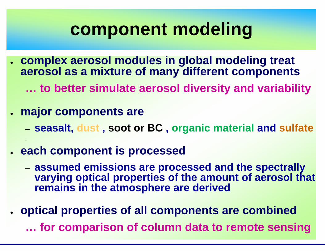
component modeling● complex aerosol modules in global modeling treat

aerosol as a mixture of many different components… to better simulate aerosol diversity and variability

● major components are– seasalt, dust , soot or BC , organic material and sulfate–

● each component is processed – assumed emissions are processed and the spectrally

varying optical properties of the amount of aerosol that remains in the atmosphere are derived

● optical properties of all components are combined… for comparison of column data to remote sensing

models like to please AOD

0

0.04

0.08

0.12

0.16

LO LS UL SP CT MIEH NF OT OG IM GM GO GITM GR NM NC Ae S*

annu

al g

loba

l aot

all

SS

DU

POM

BC

SU

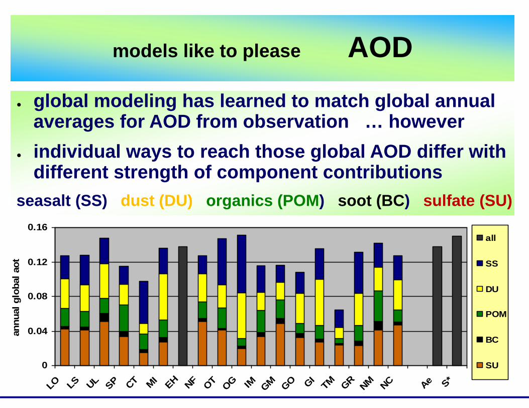
● global modeling has learned to match global annual averages for AOD from observation … however

● individual ways to reach those global AOD differ with different strength of component contributions

seasalt (SS) dust (DU) organics (POM) soot (BC) sulfate (SU)

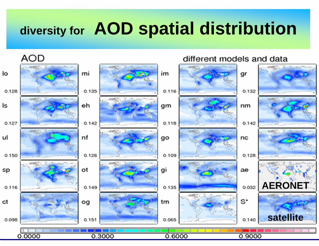
diversity for AOD spatial distribution

AERONET

satellite

understanding differences ?● model input (assumed component emissions) could

be a main reason... however, simulations with harmonized emissions did not have a major influences on component AOD biases

● aerosol processing (e.g. transport, removal, chemistry) seems the major driver for model diversity… and to make things worse, assumed processes lack validation (at least at modeling scales) no obs constrains

● QUESTION: how is the aerosol removal of aerosol components treated in aerosol modules? Is there agreement ? Is there diversity ? If so, how bad ?

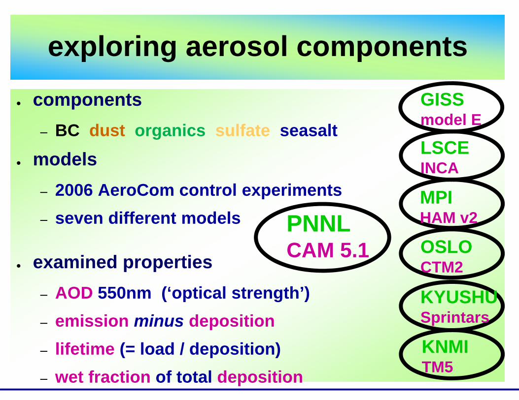
exploring aerosol components● components

– BC dust organics sulfate seasalt● models

– 2006 AeroCom control experiments– seven different models

● examined properties– AOD 550nm (‘optical strength’)– emission minus deposition– lifetime (= load / deposition)– wet fraction of total deposition

MPIHAM v2

GISSmodel E

LSCEINCA

OSLOCTM2

KYUSHUSprintars

KNMITM5

PNNLCAM 5.1

exploration by component● AOD

– spread indicates transport

● EMISSION (‘P’) minus DEPOSITION (‘L’)– separating P-areas, L-areas and ‘deserts’

● Lifetime– focus on differences in P- and L-areas

● WET deposition FRACTION (of total deposition)– Are there clouds? Is mixing inhibited (inversions)?

BC summary

● AOD maxima over S/E Asia and wildfire regions● strong differences in transport and deposition also

effect global AOD averages and distribution ● shorter lifetime near sources and longer lifetimes

over stratocumulus decks, where mixing of elevated BC aerosol in inhibited and where wet deposition fractions are lower.

● P near sources and L in outflow regions close by. Vast regions with very small L large lifetimes

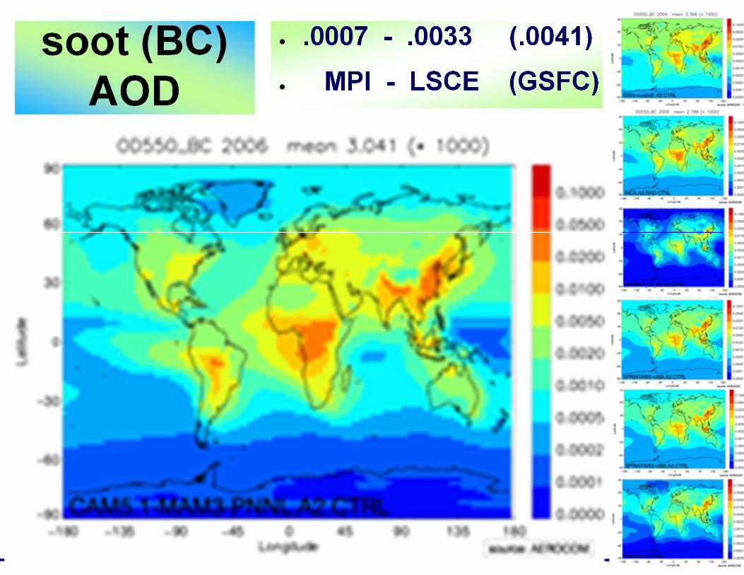
soot (BC) AOD

● .0007 - .0033 (.0041)● MPI - LSCE (GSFC)

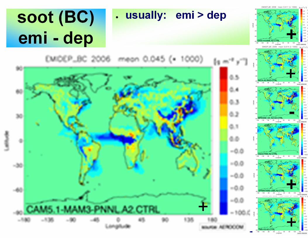
soot (BC) emi - dep

● usually: emi > dep

+

+

-

++

+

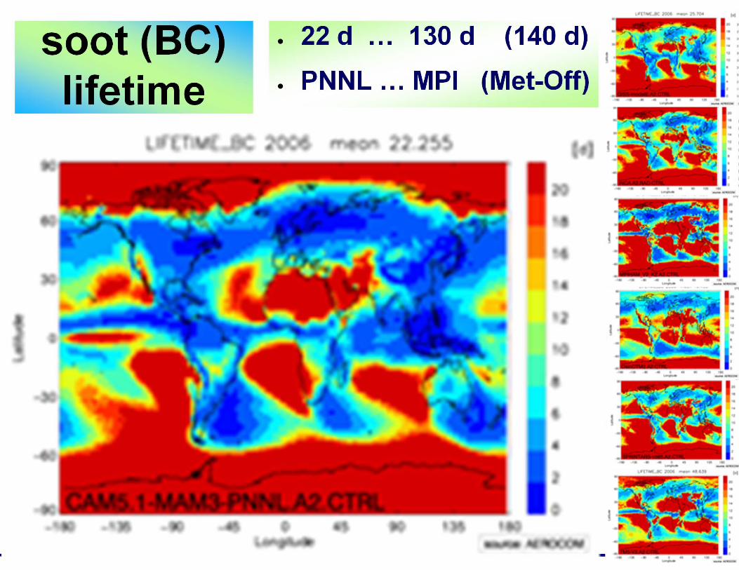
soot (BC) lifetime

● 22 d … 130 d (140 d)● PNNL … MPI (Met-Off)

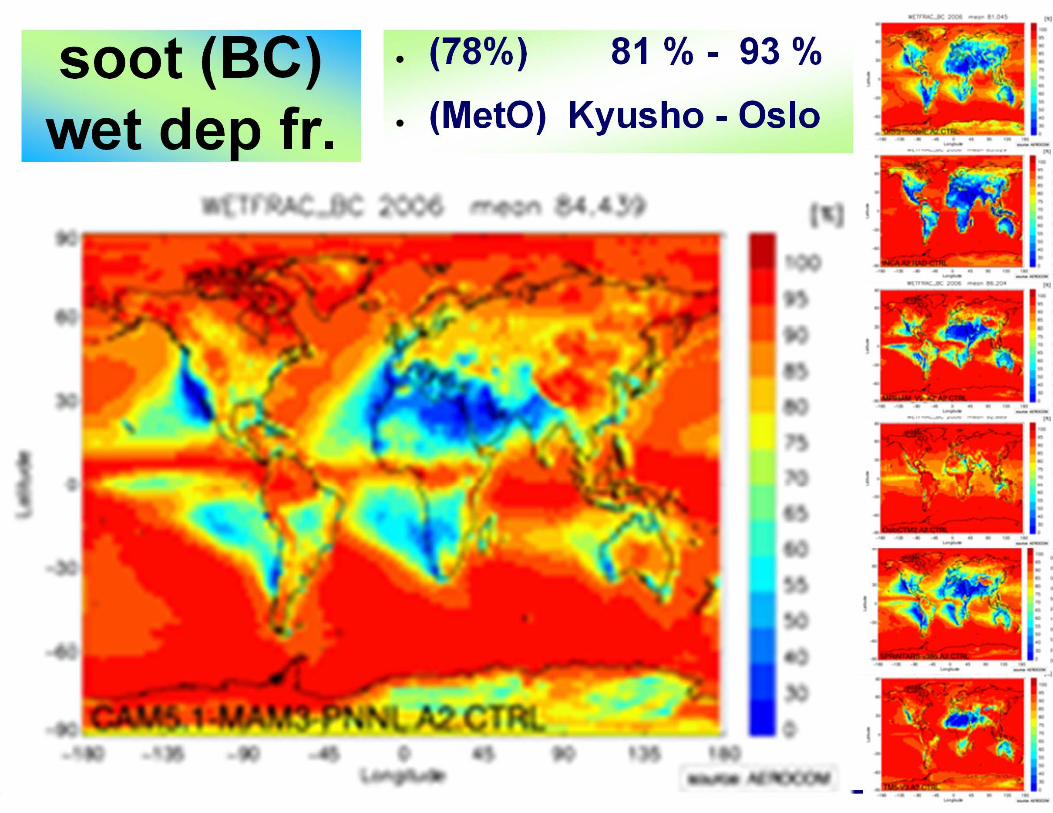
soot (BC) wet dep fr.

● (78%) 81 % - 93 %● (MetO) Kyusho - Oslo

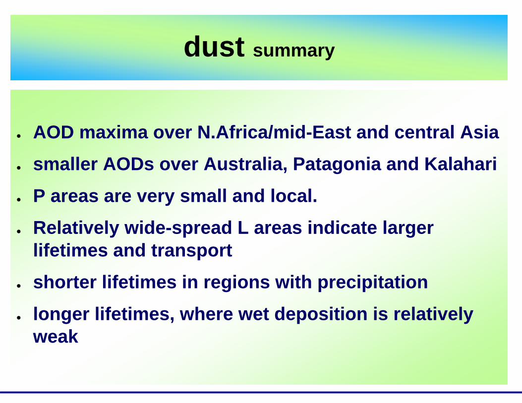
dust summary

● AOD maxima over N.Africa/mid-East and central Asia● smaller AODs over Australia, Patagonia and Kalahari ● P areas are very small and local.● Relatively wide-spread L areas indicate larger

lifetimes and transport● shorter lifetimes in regions with precipitation ● longer lifetimes, where wet deposition is relatively

weak

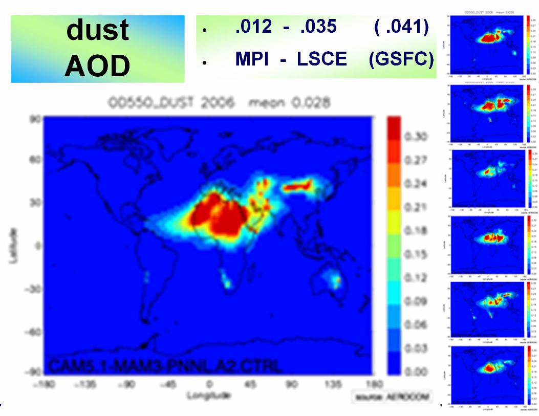
dust AOD

● .012 - .035 ( .041)● MPI - LSCE (GSFC)

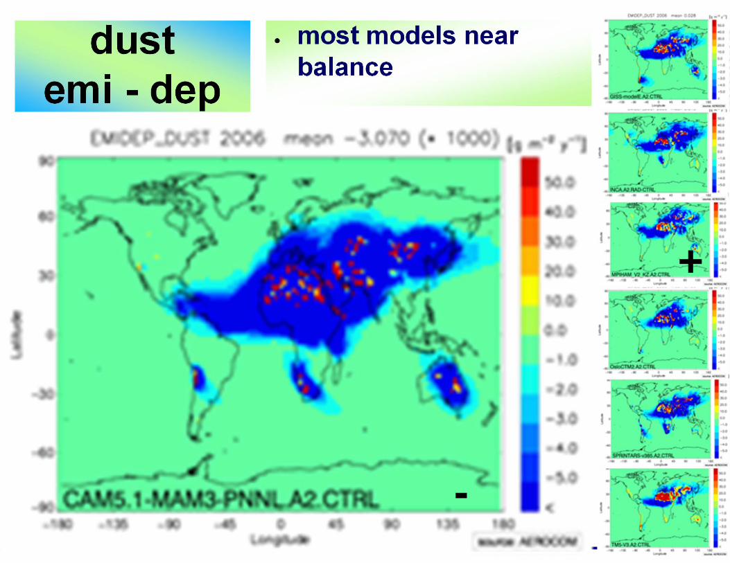
dust emi - dep

● most models near balance

+

-

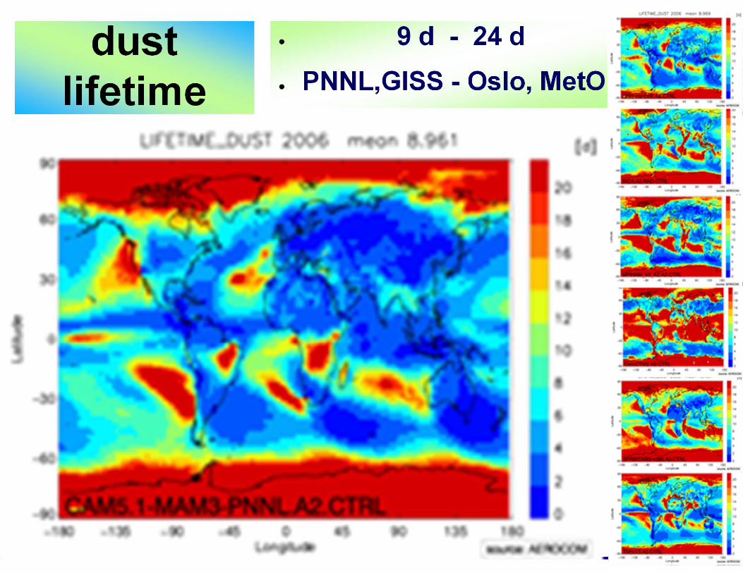
dust lifetime

● 9 d - 24 d● PNNL,GISS - Oslo, MetO

dust wet dep fr.

● 60 % - 80 %● Kyushu - Oslo

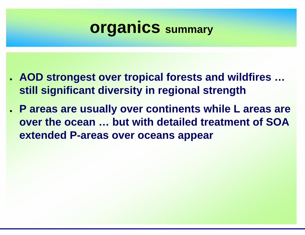
organics summary

● AOD strongest over tropical forests and wildfires … still significant diversity in regional strength

● P areas are usually over continents while L areas are over the ocean … but with detailed treatment of SOA extended P-areas over oceans appear

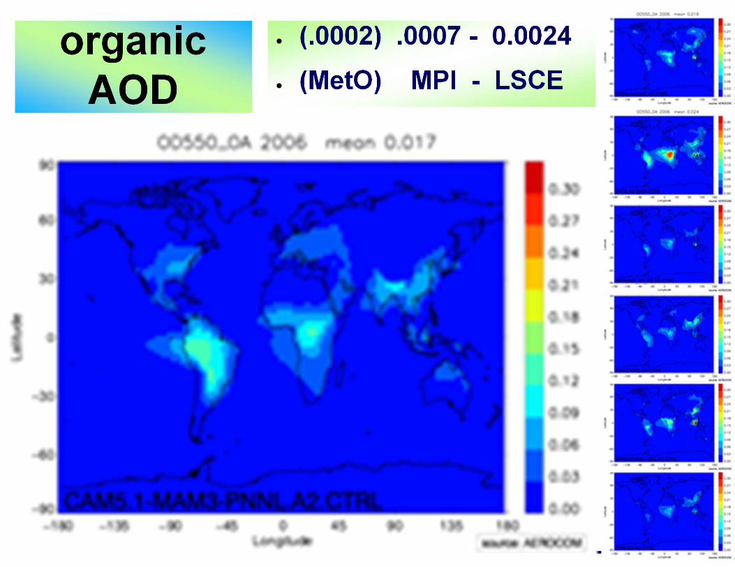
organic AOD

● (.0002) .0007 - 0.0024● (MetO) MPI - LSCE

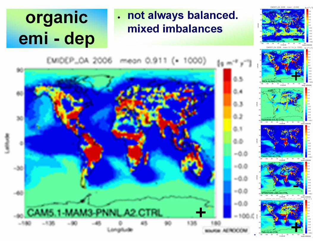
organic emi - dep

● not always balanced. mixed imbalances

++

+

-

-

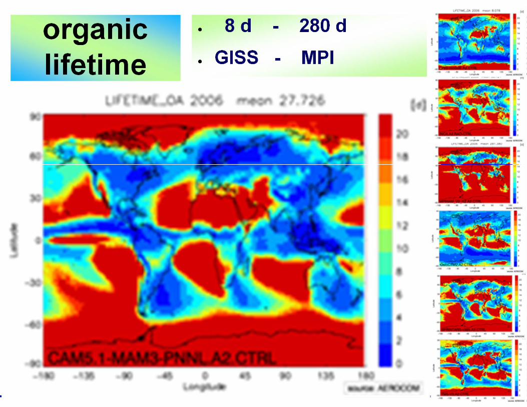
organic lifetime

● 8 d - 280 d● GISS - MPI

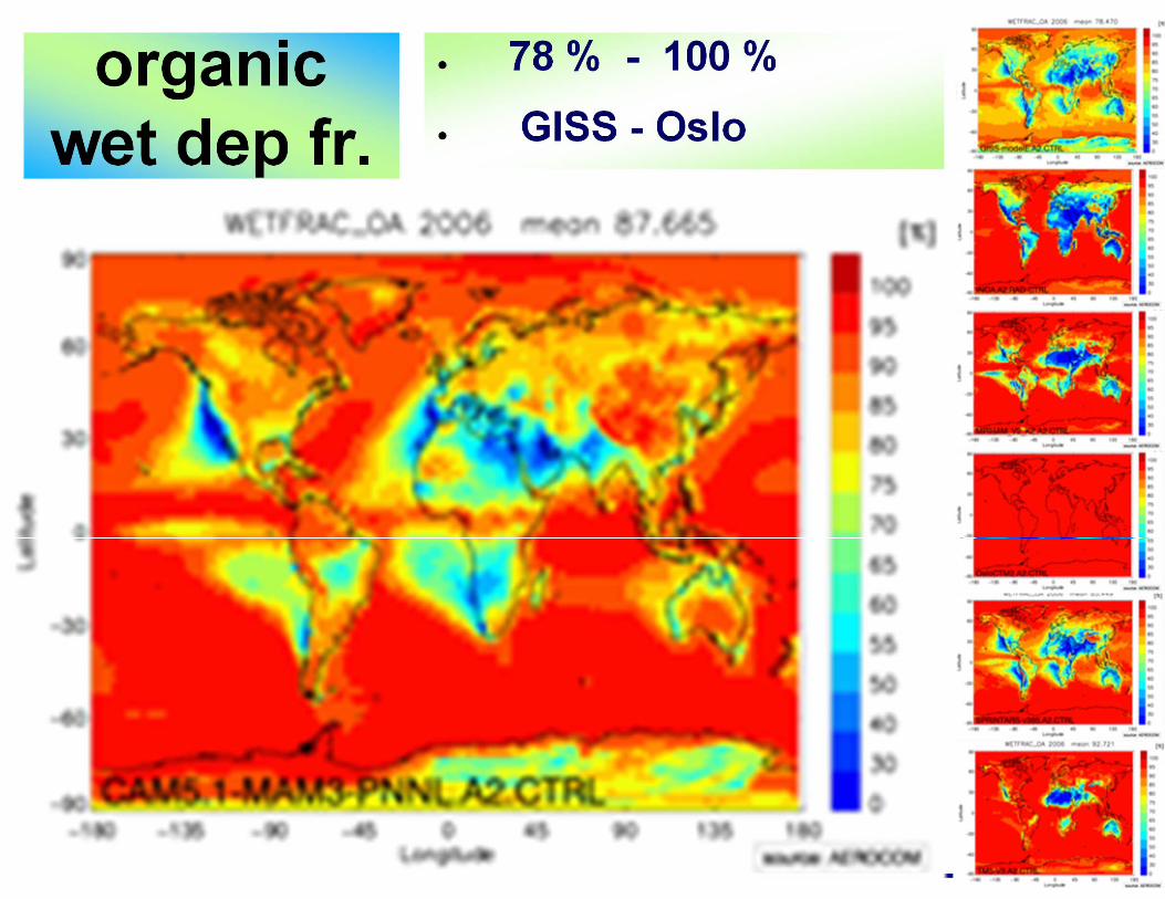
organic wet dep fr.

● 78 % - 100 %● GISS - Oslo

sulfate summary

● AOD maxima over (NH) urban industrial regions● Models with ‘easier’ transport display larger AOD● Regional wet deposition fraction patterns similar to

OA, but shorter lifetimes than OA● SO4 deposition analysis is difficult, as it is often not

clear inhowfar in individual models contribution from DMS and SO2 are included

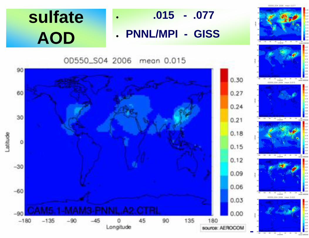
sulfate AOD

● .015 - .077● PNNL/MPI - GISS

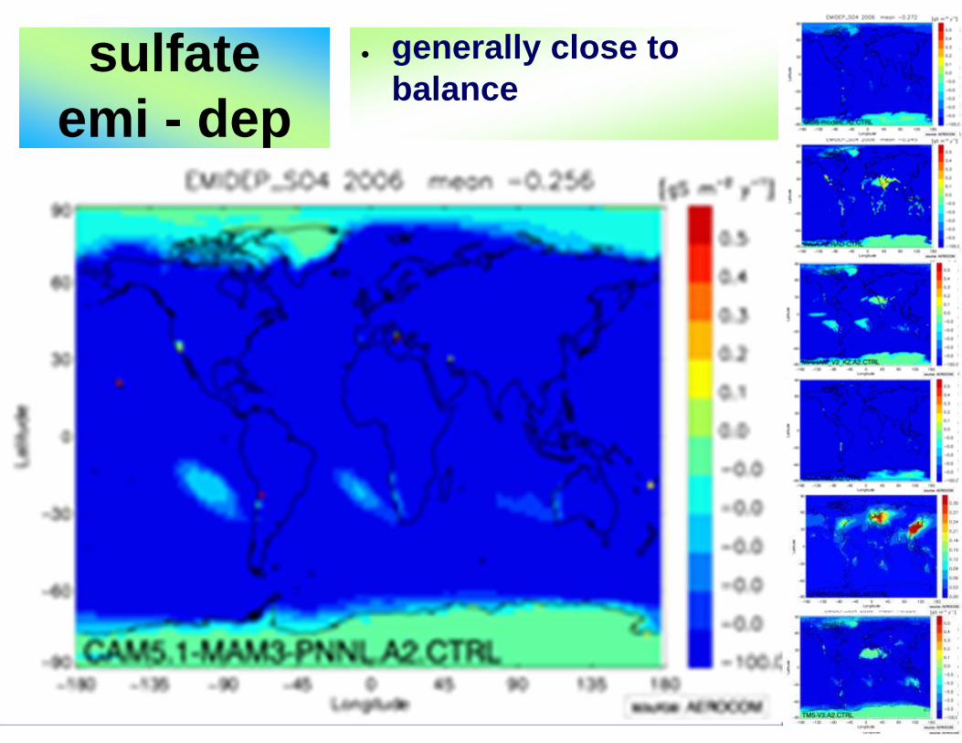
sulfate emi - dep

● generally close to balance

+

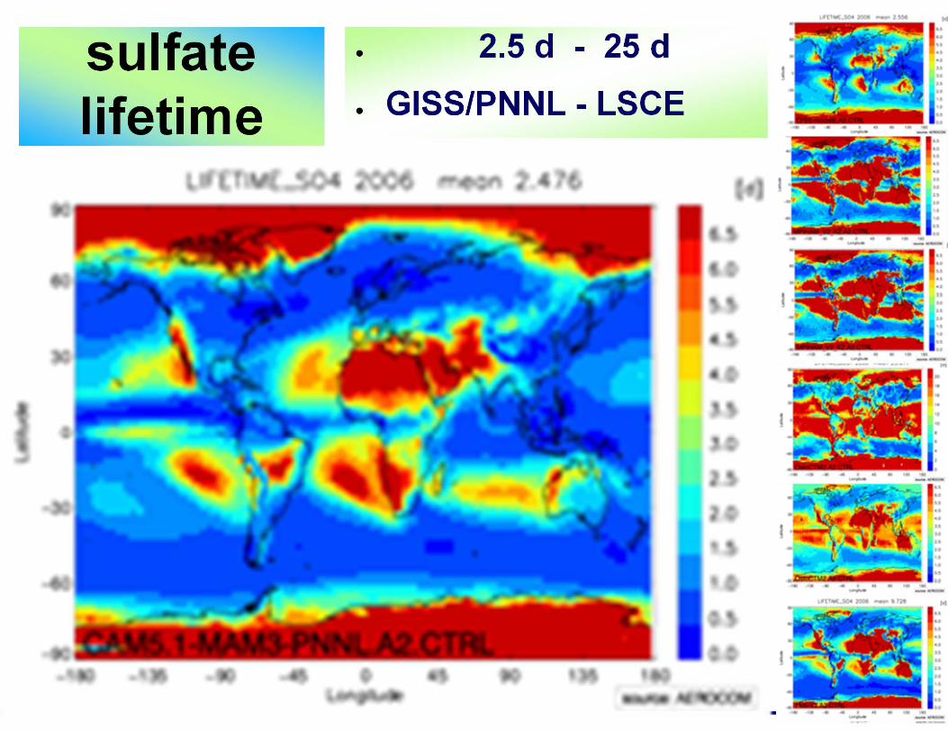
sulfate lifetime

● 2.5 d - 25 d● GISS/PNNL - LSCE

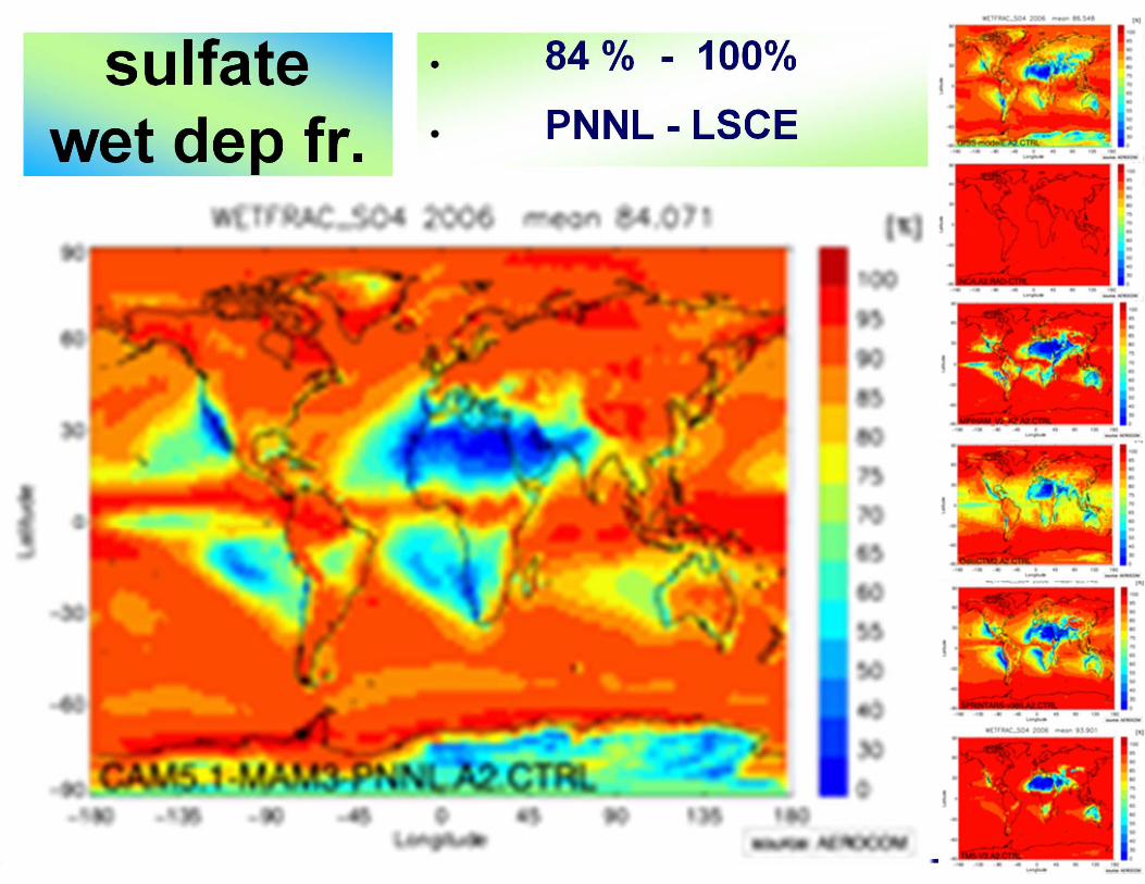
sulfate wet dep fr.

● 84 % - 100%● PNNL - LSCE

sea-salt summary

● huge diversity in AOD and location od AOD maxima … in part due to the strong ‘slave’ dependence on carrier model properties (rel. humidity, surface winds)

● relatively (also to all other aerosol components) low wet deposition fraction – only larger over continents and the ITCZ

● apparently, sea-salt modeling has received less attention, possibly because it is not ‘anthropogenic’, has a small greenhouse effect and is over oceans

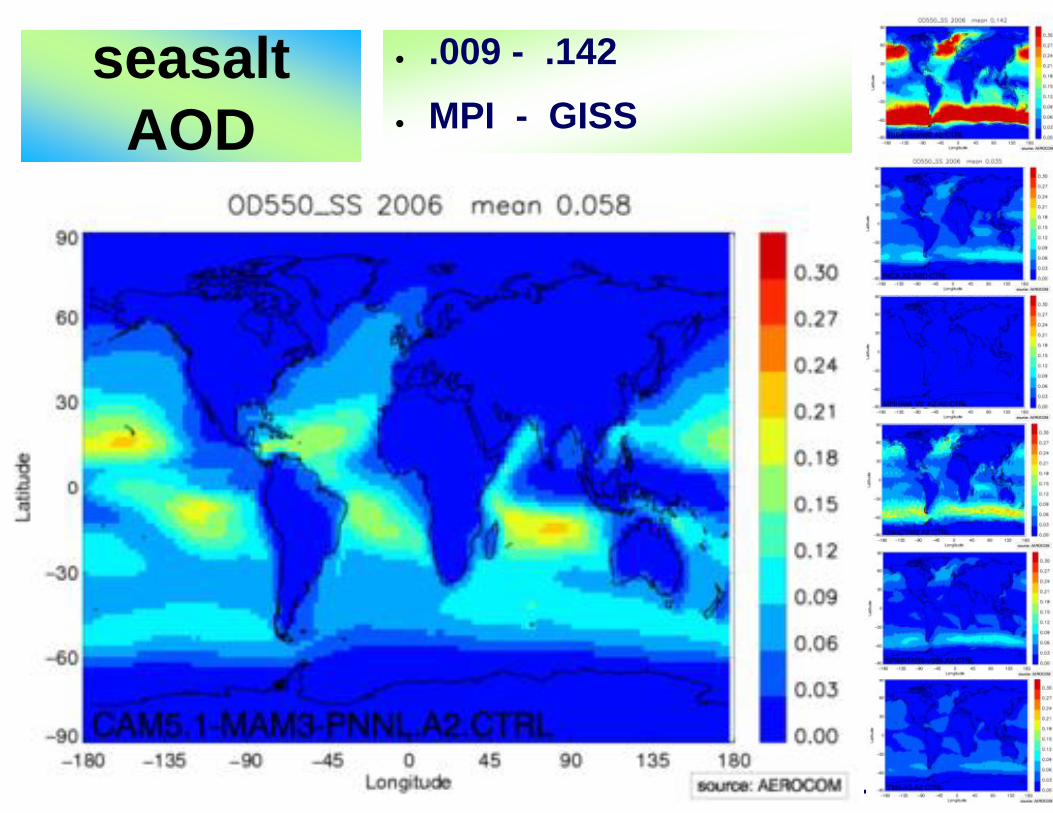
seasalt AOD

● .009 - .142● MPI - GISS

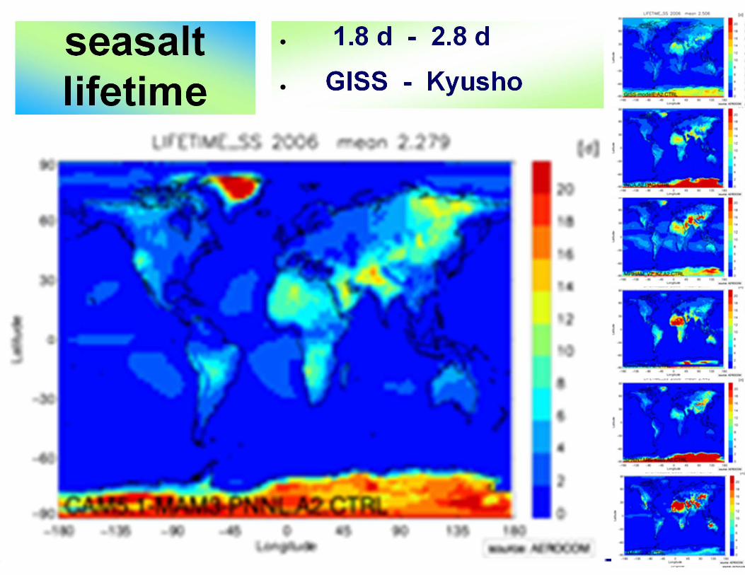
seasalt lifetime

● 1.8 d - 2.8 d● GISS - Kyusho

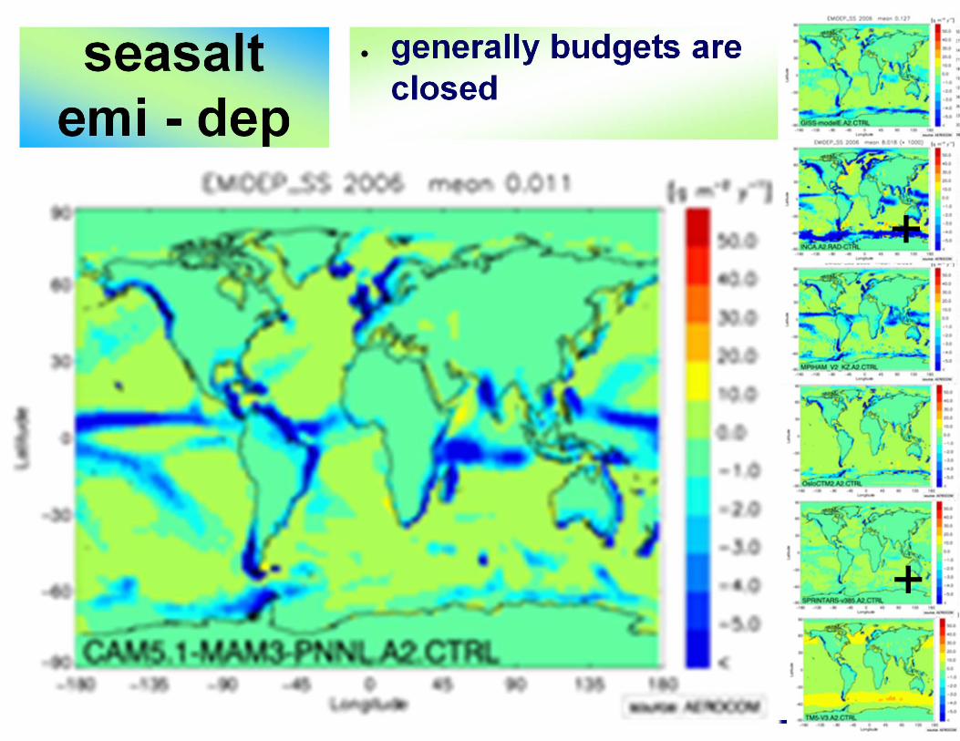
seasalt emi - dep

● generally budgets are closed

+

+

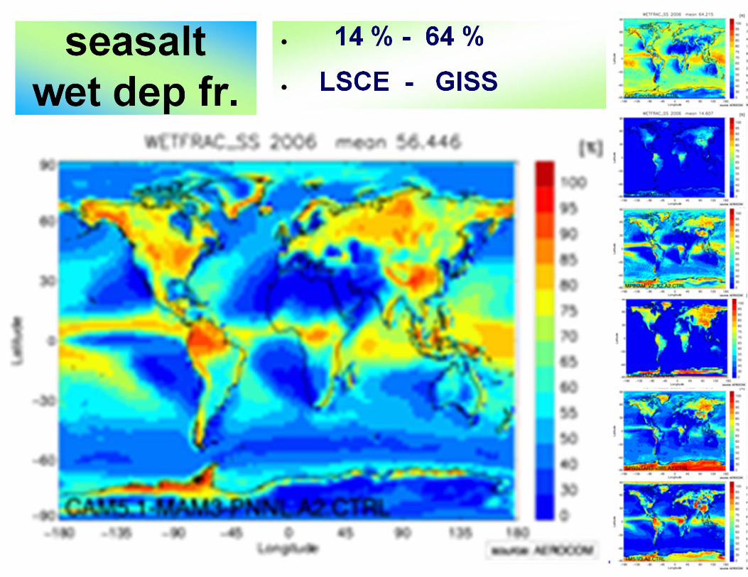
seasalt wet dep fr.

● 14 % - 64 %● LSCE - GISS

resource - all and more● MetNo webpage

– data from more models and different experiments are ready to be viewed …

– http://aerocom.met.no/cgi-bin/aerocom/surfobs_annualrs.pl

● any volunteer (e.g. master student) is invited to look at the many plots and budgets– I doubt that many modelers have intensely looked at

their model performance in detail (which they should)

● median model (and central diversity for confidence ) – to be established for all properties as general reference

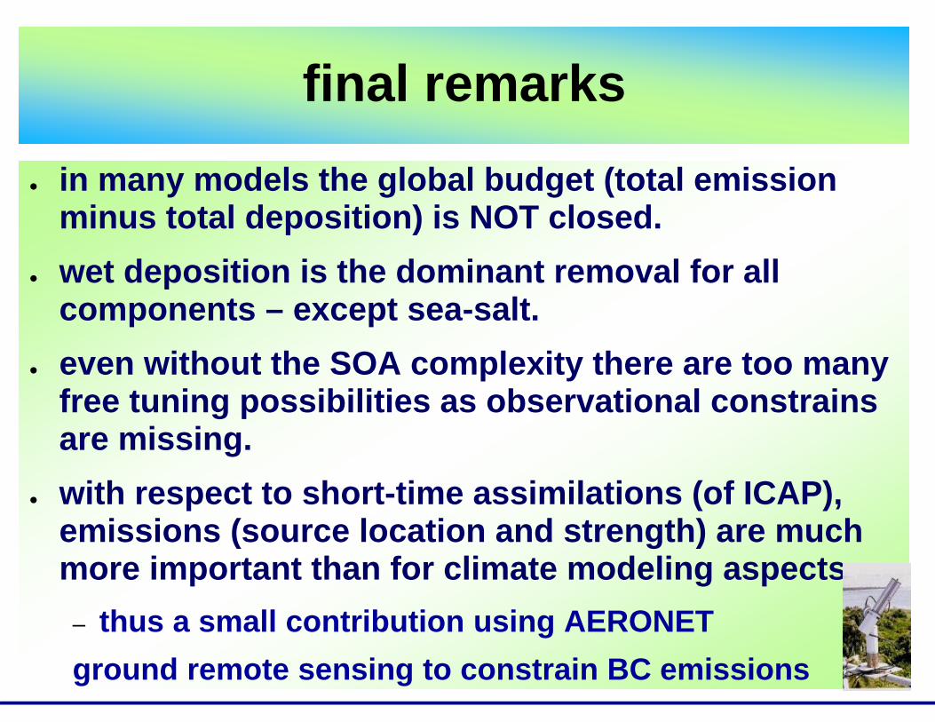
final remarks● in many models the global budget (total emission

minus total deposition) is NOT closed.● wet deposition is the dominant removal for all

components – except sea-salt. ● even without the SOA complexity there are too many

free tuning possibilities as observational constrains are missing.

● with respect to short-time assimilations (of ICAP), emissions (source location and strength) are much more important than for climate modeling aspects– thus a small contribution using AERONET ground remote sensing to constrain BC emissions

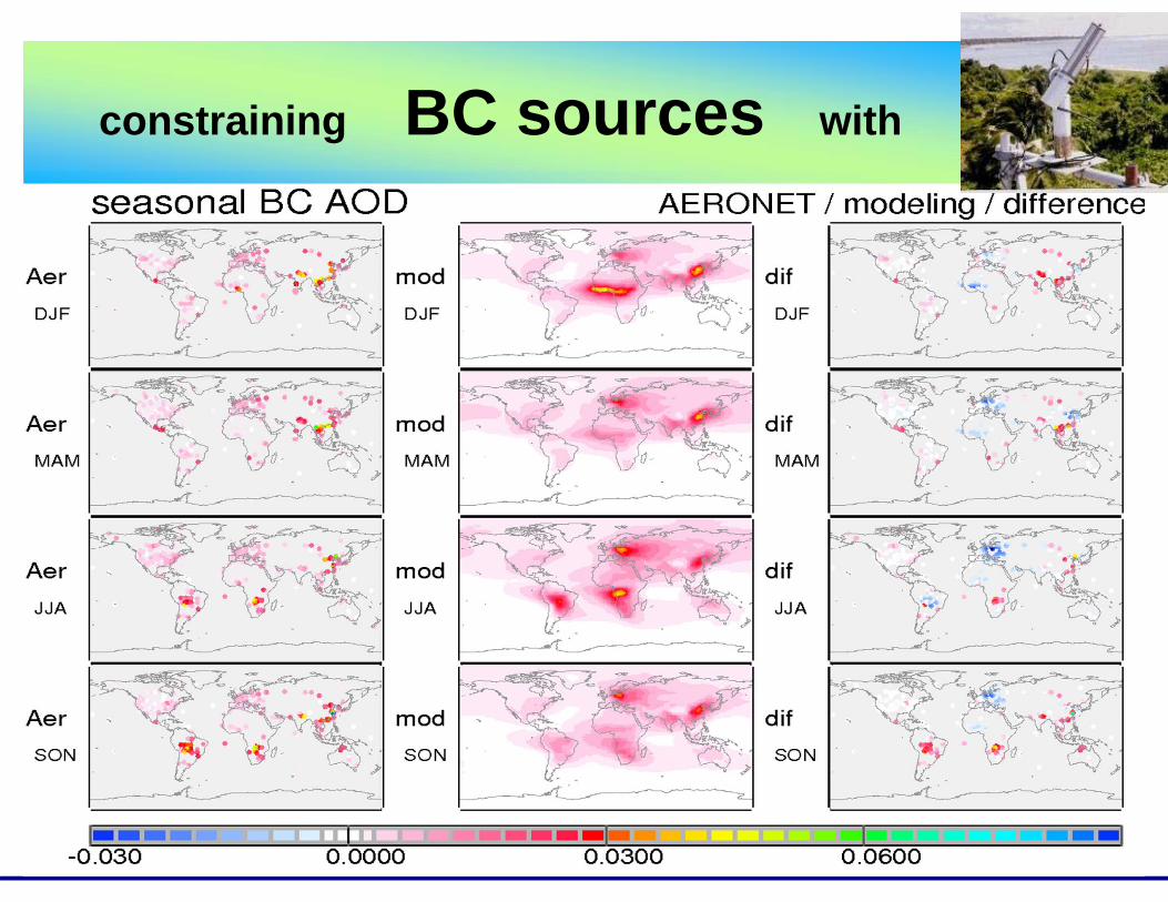
constraining BC sources with

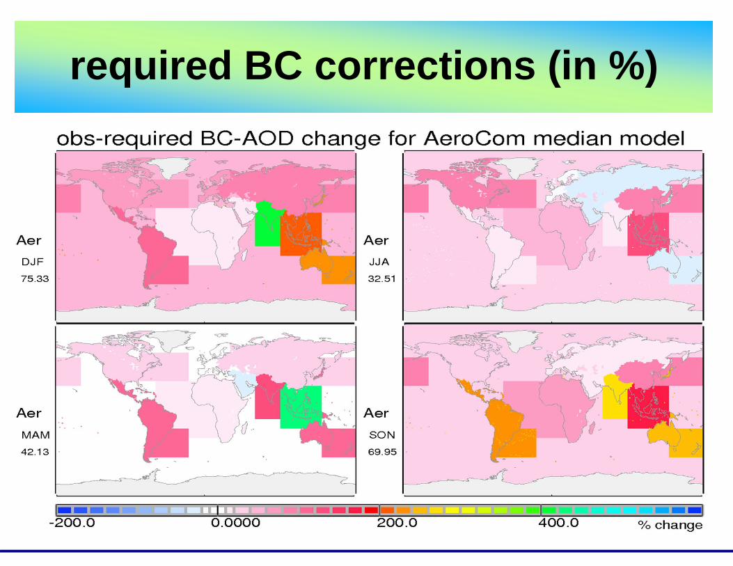
required BC corrections (in %)