Parallel Implementation of the Bi-CGSTAB

Method with Block Red-Black Gauss-Seidel

Preconditioner Applied to the Hermite

Collocation Discretization of Partial

Di�erential Equations

Stephen H. Brill

Department of Mathematics, Boise State University, Boise, Idaho, U.S.A.

George F. Pinder

Department of Civil and Environmental Engineering, University of Vermont,

Burlington, Vermont, U.S.A.

Abstract

We describe herein the parallel implementation of the Bi-CGSTAB method witha block Red-Black Gauss-Seidel (RBGS) preconditioner applied to the systems oflinear algebraic equations that arise from the Hermite collocation discretization ofpartial di�erential equations in two spatial dimensions. The method is implementedon the Cray T3E, a parallel processing supercomputer. Speedup results are dis-cussed.

Key words: Hermite collocation, Bi-CGSTAB, preconditioner, speedup

1 Introduction

We are concerned with the rapid solution of matrix equations which arise fromthe Hermite collocation discretization of partial di�erential equations (PDEs)in two spatial dimensions. This discretization is attractive for several reasons,including

.

.

Preprint submitted to Elsevier Preprint 10 September 2001

� the freedom in how one numbers equations and unknowns, thus being ableto manipulate to best advantage the structure of the resulting matrix (thispoint is discussed in greater detail in Section 3 below);

� the freedom in how one locates the \collocation points," which can acceleratethe rate at which convergence to the solution occurs (see [4] and [5]); and

� the spline that represents the solution has a continuous �rst derivative.This last property can be he helpful in modeling subsurface multiphase owproblems, like those in [12].

In general, the matrix arising from the Hermite collocation discretization doesnot enjoy many pleasant properties of matrices arising from other populardiscretizations (e.g., �nite di�erences or �nite elements). In particular, collo-cation matrices are not diagonally dominant, not positive de�nite, and notsymmetric (even in the case of symmetric di�erential operators).

To solve these matrix equations, the two most widely used approaches arethe GMRES [20] and Bi-CGSTAB [22] methods. For this work, we choose theBi-CGSTAB method for two reasons. First, the Bi-CGSTAB method lendsitself more readily to parallel processing than does GMRES. Also, there isevidence ([2], [7], [21], [23]) that Bi-CGSTAB is superior for a large class ofproblems. We combine Bi-CGSTAB with a Red-Black numbering system andpreconditioning matrix which facilitates use of the Bi-CGSTAB method in aparallel processing mode. It was shown in [2] that BiCGSTAB/RBGS is ane�ective serial (i.e., not parallel) method for solving such matrix equations.

In [1], a parallel method based on fast Fourier transforms (FFTs) for solv-ing PDEs discretized by Hermite collocation is presented. However, the FFTmethod is limited by requiring the same uniform mesh in both coordinate di-mensions (our technique allows nonuniform meshes and the meshes in the twocoordinate dimensions may be di�erent) and the PDEs amenable to the FFTmethod are less general than those amenable to ours.

A multisplitting method designed for parallel processing is implemented in [18]for solving Poisson's equation discretized by Hermite collocation. Other e�ortscombining parallel processing with collocation include [8] and [9], which usesquadratic, rather than cubic, basis functions; [12], which uses an alternatingdirection solver; and [13], where the focus is on describing a method for coarsegrain partitioning applied to PDE problems.

In addition, the PIM (Parallel Iterative Methods) [10] software package forsolving linear systems deserves mention. PIM requires the user to select aniterative method (choices include Bi-CGSTAB and GMRES) and then to in-terface his/her own code with that of PIM. The user must supply code formatrix-vector multiplication, solving preconditioned linear systems, vector in-

2

ner products, and computation of vector norms. For the case of GMRES, usingPIM would result in substantially less e�ort on the part of the user to pro-duce working code. However, the only components of Bi-CGSTAB that theuser would not have to write himself/herself are routines for vector addition(and subtraction), the multiplication of a vector by a scalar, and scalar arith-metic. Since these are easily written, using PIM in conjunction with our codeis hardly worthwhile.

In general, Krylov methods (like GMRES and Bi-CGSTAB) are usually foundto be superior to \splitting" methods, in terms of minimizing solving time.Thus, based on evaluation of the literature, we believe our method to be thefastest, most general one available for solving collocation matrix equations,even when implemented serially. This last point is relevant to the discussionin Section 5.4.

This paper is organized as follows. After a brief introduction to collocation, weintroduce the Red-Black numbering scheme and our preconditioning matrix.After then discussing the parallel implementation of the Bi-CGSTAB with ourpreconditioner, we provide speedup results. A short section summarizing ourwork concludes the paper.

2 Collocation in two spatial dimensions

In this section we provide a brief overview of collocation in two spatial dimen-sions. For a thorough development, see [3].

We are concerned with the numerical solution of the PDE

L [u] (x; y) = A (x; y)@2u

@x2+B (x; y)

@2u

@x@y+ C (x; y)

@2u

@y2

+D (x; y)@u

@x+ E (x; y)

@u

@y+ F (x; y)u = H (x; y)

(1)

on the domain D = [ax; bx] � [ay; by] with Dirichlet or Neumann boundaryconditions. UponD we impose a rectilinear mesh of rectangular �nite elements.Let mx and my be the number of �nite elements in the x- and y-directions,respectively. (Throughout this work, we assume that my is even.)

The collocation discretization proceeds by introducing a piecewise Hermitebi-cubic interpolating polynomial �u into (1), resulting in

L [�u] (x; y)�H (x; y) = � (x; y) ;

3

where � (x; y) is an error function. We then enforce

� (x; y) = 0 (2)

at four distinct collocation points within the interior of each rectangular �-nite element. Since there are mxmy �nite elements, we are de�ning 4mxmy

equations by enforcing (2) at the collocation points. In this work, we let thecollocation points coincide with the points of Gaussian quadrature, a choicethat, given certain smoothness conditions, minimizes truncation error [19].

The degrees of freedom (dofs) of �u are approximations to u, @u@x, @u@y, and @2u

@x@y

at the (mx + 1)(my + 1) nodes (i.e., corners of the �nite elements). Afterintroducing boundary conditions, we are left with 4mxmy unknown degrees offreedom. Since we have 4mxmy equations from enforcing (2) at the collocationpoints, we can determine the unknown coeÆcients.

3 The Red-Black ordering scheme

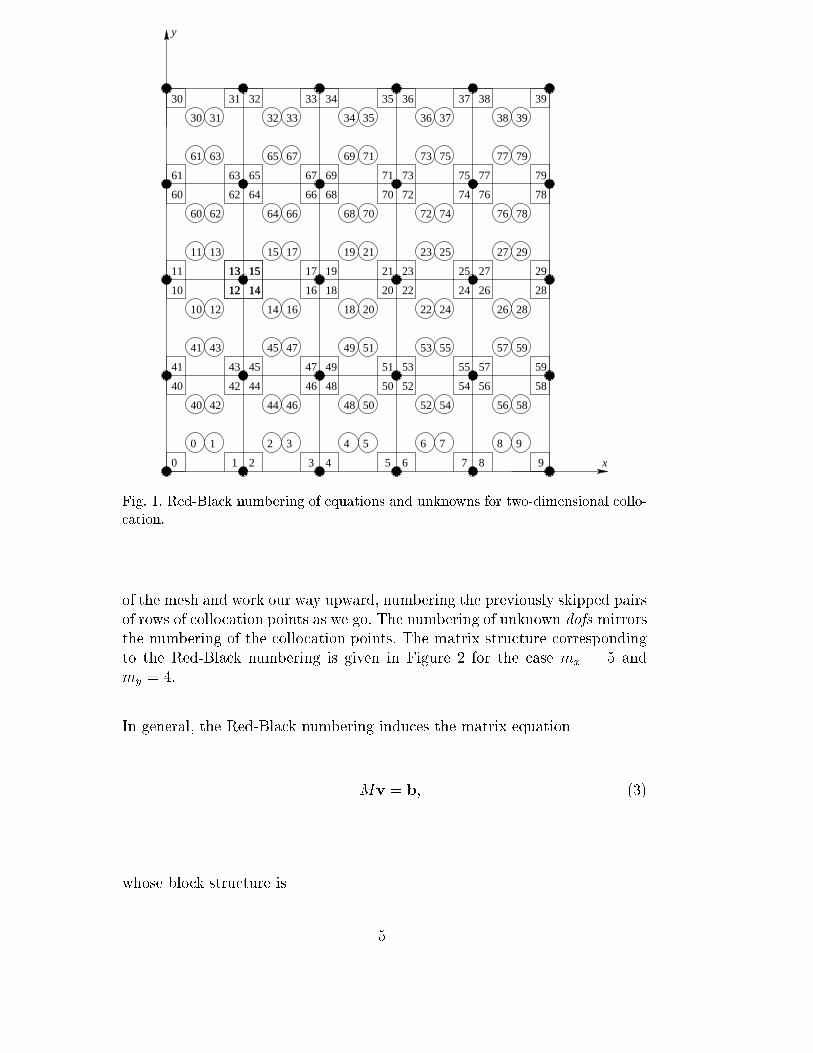
Collocation provides freedom in how one orders the equations and unknowns.In the literature, the most popular numbering provides a block tridiagonalstructure, as implemented in [11], [16], and [17]. In this work (and previouslyin [2] and [6]), we permute the block tridiagonal numbering to arrive at ourRed-Black ordering, depicted in Figure 1 for the case mx = 5 and my = 4.

In Figure 1, we have 20 (= mxmy) rectangular �nite elements; at each cornerof each �nite element is a node (depicted by a �lled-in circle). At each node arefour dofs. However, only the interior nodes are depicted as having four dofs.This is because each node on the boundary has fewer than four unknown dofsassociated with it due to the imposition of boundary conditions. In particular,the boundary nodes have two unknown dofs each with the exception of thosenodes at the four corners of the domain, which have one unknown dof each.Each of these unknown dofs is depicted by an integer (from 0 to 79 (= 4mxmy�1)) inside a small square adjacent to the node with which it is associated. Inaddition, in the interior of each of the 20 �nite elements are four collocationpoints, each depicted by a circle with an integer (between 0 and 79 also) inside.

With reference to Figure 1, the Red-Black ordering proceeds by numbering (inascending order and from left to right) the bottom row of collocation points,then skipping two rows of collocation points, then resuming the numberingwith the next two rows of collocation points. This pattern of skipping andthen numbering pairs of rows of collocation points continues until we reachthe top of the mesh where, since my must be even, we have a single row ofcollocation points remaining, which we number. We then return to the bottom

4

29

2810

11

41

40

59

58

79

78

61

60

y

x

��������

��������

��������

��������

��������

��������

��������

��������

��������

��������

��������

��������

��������

��������

��������

��������

��������

��������

��������

��������

��������

��������

��������

��������

��������

��������

��������

��������

��������

��������

0 1 2 3 4 5 6 7 8 9

10 12 14 16 18 20 22 24 26 28

11 13 15 17 19 21 23 25 27 29

42 4640 44 48 565250 54 58

62 6660 64 68

43 4741 45 49 575351 55 59

63 6761 65 69

30 31 32 33 34 35 36 37 38 39

70

71

72

73

74

75

76

77

78

79

90

12 14

13 15

12 14

13 15

24 26

25 27

20 2216 18

17 19 21 23

30 31 32 35 36 3933 34 37 38

42 44

43 45

46 48

47 49

50 52

51 53

54 56

55 57

74 76

75 77

70 72

71 73

66 68

67 69

62 64

63 65

1 2 3 4 5 6 7 8

Fig. 1. Red-Black numbering of equations and unknowns for two-dimensional collo-cation.

of the mesh and work our way upward, numbering the previously skipped pairsof rows of collocation points as we go. The numbering of unknown dofs mirrorsthe numbering of the collocation points. The matrix structure correspondingto the Red-Black numbering is given in Figure 2 for the case mx = 5 andmy = 4.

In general, the Red-Black numbering induces the matrix equation

Mv = b; (3)

whose block structure is

5

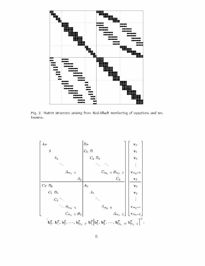
Fig. 2. Matrix structure arising from Red-Black numbering of equations and un-knowns.

266666666666666666666666666664

AF BF

A1 C0 B1

A3 C2 B3

. . .. . .

. . .

Amy�3 Cmy�4 Bmy�3

AL CL

CF B0 A0

C1 B2 A2

C3

. . .. . .

. . . Bmy�4 Amy�4

Cmy�3 BL Amy�2

377777777777777777777777777775

266666666666666666666666666664

vF

v1

v3

...

vmy�3

vL

v0

v2

...

vmy�4

vmy�2

377777777777777777777777777775

=hbTF ; b

T1; bT

3; � � � ; bTmy�3

; bTL bT0; bT

2; � � � ; bTmy�4

; bTmy�2

iT;

6

which we abbreviate264R U

L B

375264 vRvB

375 =

264 bRbB

375 : (4)

(The symbols R and B in (4) may, respectively, be considered to stand for\red" and \black".) As discussed earlier, matrix M is not symmetric, notpositive de�nite, and not diagonally dominant.

4 Our preconditioning matrix

As with any Krylov method (like Bi-CGSTAB), the fastest convergence isobtained via the use of an appropriate \preconditioning" matrixQ. The matrixQ is chosen such that Q � M and that linear systems of the form Qy = c areeasy to solve. For our purposes, we stipulate a third requirement: Q must havea structure amenable to parallel processing. With respect to (4), we chooseour preconditioning matrix Q to be

Q =

264RL B

375 : (5)

We note that this is the matrix corresponding to implementing a block Gauss-Seidel method to solve (3).

There are, of course, other possible choices for the preconditioning matrixQ. One is the incomplete block LU preconditioner which, as studied in [2],compares most unfavorably to Q. A block Jacobi preconditioner is anotheroption, but would be expected to perform poorly because the matrix M is farfrom being block diagonally dominant.

A possible drawback of using our Red-Black numbering scheme is that theconvergence of \splitting" methods (like Jacobi, Gauss-Seidel, SOR, etc.) isknown to be adversely a�ected by such numberings [15]. However, this draw-back does not apply directly to our case, since we are not using a splittingmethod. Rather, we are using the matrix corresponding to a splitting method(in this case, Gauss-Seidel) as a preconditioner within a Krylov method.

As is evident from Section 5.3 below, it is precisely the Red-Black numbering,combined with the block Gauss-Seidel preconditioning matrix Q, that allowsus to distribute our data evenly among the various processors and to easily ex-ecute Bi-CGSTAB in parallel. While the block tridiagonal numbering of [11],

7

[16], and [17], discussed at the beginning of Section 3, permits the identicaldistribution of data among processors, the corresponding block Gauss-Seidelpreconditioning matrix, lacking the Red-Black structure, does not permit sim-ple parallelization. One could, of course, use a block Jacobi preconditioner inconjunction with the block tridiagonal ordering to achieve parallelization, butthis su�ers from the drawback discussed above.

5 Parallel implementation

In this section, we discuss the implementation of the Bi-CGSTAB methodwith our preconditioner on the Cray T3E, a parallel processing supercom-puter. (Source code is available at [24].) After describing how each entry ofM , v, and b is assigned to its particular processor, we brie y discuss theissue of which parallel processing architecture should be chosen. We next de-tail the parallel implementation of those operations in the Bi-CGSTAB/RBGSalgorithm which require interprocessor communication. (The operations in Bi-CGSTAB/RBGS that do not require interprocessor communication parallelizein a straightforward and obvious manner.) We then give speedup results.

In this work, we will assume that my, the number of �nite elements in they-direction, is a multiple of p, the number of processors.

5.1 The allocation of portions of M , v and b to the various processors

We illustrate the ideas in this subsection using the particular case my = 16and p = 4. The general case will then be transparent.

Let the p = 4 processors be denoted P1, �P2, _P3, and �P4. For the case wheremy = 16, we have v, b and the blocks of M (i.e., R, U , L, and B) given by

v =�vTF ; v

T1; �vT

3; �vT

5; _vT

7; _vT

9; �vT

11; �vT

13; vL vT

0; vT

2; �vT

4; �vT

6; _vT

8; _vT

10; �vT

12; �vT

14

�T;

b =�bTF ; b

T1; �bT

3; �bT

5; _bT

7; _bT

9; �bT

11; �bT

13; bL vT

0; bT

2; �bT

4; �bT

6; _bT

8; _bT

10; �bT

12; �bT

14

�T;

8

R =

2666666666666666666666666664

AF

A1

�A3

�A5

_A7

_A9

�A11

�A13

AL

3777777777777777777777777775

,

U =

2666666666666666666666666664

BF

C0 B1

C2�B3

�C4�B5

�C6_B7

_C8_B9

_C10�B11

�C12�B13

�CL

3777777777777777777777777775

,

L =

2666666666666666666666664

CF B0

C1 B2

�C3�B4

�C5�B6

_C7_B8

_C9_B10

�C11�B12

�C13�BL

3777777777777777777777775

,

9

and

B =

2666666666666666666666664

A0

A2

�A4

�A6

_A8

_A10

�A12

�A14

3777777777777777777777775

.

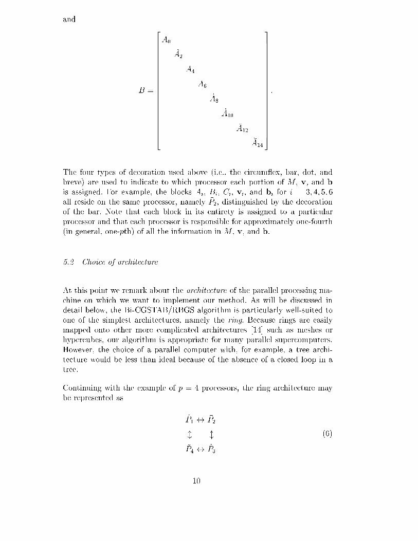
The four types of decoration used above (i.e., the circum ex, bar, dot, andbreve) are used to indicate to which processor each portion of M , v, and b

is assigned. For example, the blocks Ai, Bi, Ci, vi, and bi for i = 3; 4; 5; 6all reside on the same processor, namely �P2, distinguished by the decorationof the bar. Note that each block in its entirety is assigned to a particularprocessor and that each processor is responsible for approximately one-fourth(in general, one-pth) of all the information in M , v, and b.

5.2 Choice of architecture

At this point we remark about the architecture of the parallel processing ma-chine on which we want to implement our method. As will be discussed indetail below, the Bi-CGSTAB/RBGS algorithm is particularly well-suited toone of the simplest architectures, namely the ring. Because rings are easilymapped onto other more complicated architectures [14] such as meshes orhypercubes, our algorithm is appropriate for many parallel supercomputers.However, the choice of a parallel computer with, for example, a tree archi-tecture would be less than ideal because of the absence of a closed loop in atree.

Continuing with the example of p = 4 processors, the ring architecture maybe represented as

P1 $ �P2

l l

�P4 $ _P3

(6)

10

5.3 Parallel implementation of Bi-CGSTAB/RBGS

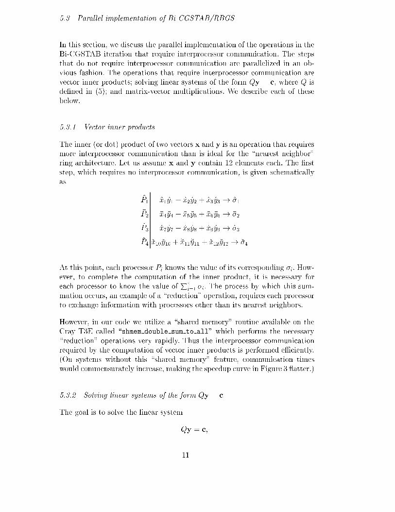
In this section, we discuss the parallel implementation of the operations in theBi-CGSTAB iteration that require interprocessor communication. The stepsthat do not require interprocessor communication are parallelized in an ob-vious fashion. The operations that require interprocessor communication arevector inner products; solving linear systems of the form Qy = c, where Q isde�ned in (5); and matrix-vector multiplications. We describe each of thesebelow.

5.3.1 Vector inner products

The inner (or dot) product of two vectors x and y is an operation that requiresmore interprocessor communication than is ideal for the \nearest neighbor"ring architecture. Let us assume x and y contain 12 elements each. The �rststep, which requires no interprocessor communication, is given schematicallyas

P1 x1y1 + x2y2 + x3y3 ! �1

�P2 �x4�y4 + �x5�y5 + �x6�y6 ! ��2

_P3 _x7 _y7 + _x8 _y8 + _x9 _y9 ! _�3

�P4 �x10�y10 + �x11�y11 + �x12�y12 ! ��4

At this point, each processor Pi knows the value of its corresponding �i. How-ever, to complete the computation of the inner product, it is necessary foreach processor to know the value of

P4

i=1 �i. The process by which this sum-mation occurs, an example of a \reduction" operation, requires each processorto exchange information with processors other than its nearest neighbors.

However, in our code we utilize a \shared memory" routine available on theCray T3E called \shmem double sum to all" which performs the necessary\reduction" operations very rapidly. Thus the interprocessor communicationrequired by the computation of vector inner products is performed eÆciently.(On systems without this \shared memory" feature, communication timeswould commensurately increase, making the speedup curve in Figure 3 atter.)

5.3.2 Solving linear systems of the form Qy = c

The goal is to solve the linear system

Qy = c,

11

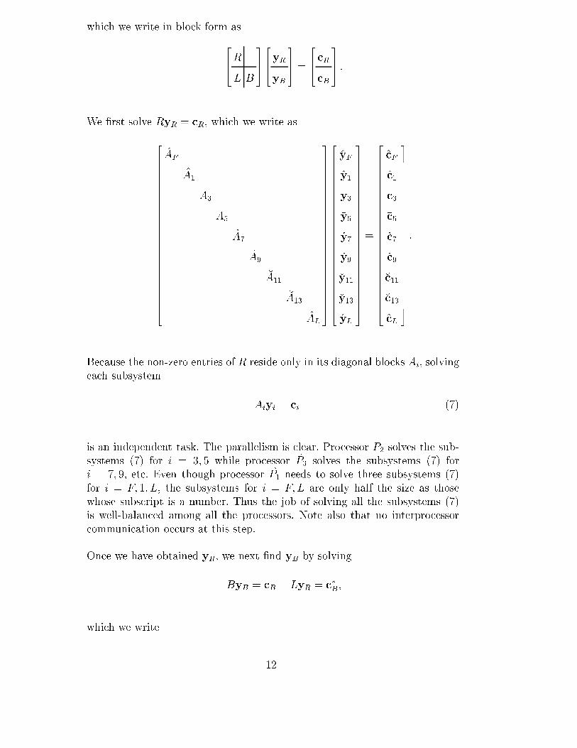
which we write in block form as

264RL B

375264 yRyB

375 =

264 cRcB

375 .

We �rst solve RyR = cR, which we write as

2666666666666666666666666664

AF

A1

�A3

�A5

_A7

_A9

�A11

�A13

AL

3777777777777777777777777775

2666666666666666666666666664

yF

y1

�y3

�y5

_y7

_y9

�y11

�y13

yL

3777777777777777777777777775

=

2666666666666666666666666664

cF

c1

�c3

�c5

_c7

_c9

�c11

�c13

cL

3777777777777777777777777775

.

Because the non-zero entries of R reside only in its diagonal blocks Ai, solvingeach subsystem

Aiyi = ci (7)

is an independent task. The parallelism is clear. Processor �P2 solves the sub-systems (7) for i = 3; 5 while processor _P3 solves the subsystems (7) fori = 7; 9, etc. Even though processor P1 needs to solve three subsystems (7)for i = F; 1; L, the subsystems for i = F; L are only half the size as thosewhose subscript is a number. Thus the job of solving all the subsystems (7)is well-balanced among all the processors. Note also that no interprocessorcommunication occurs at this step.

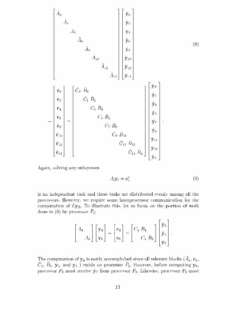
Once we have obtained yR, we next �nd yB by solving

ByB = cB � LyR = c�B,

which we write

12

2666666666666666666666664

A0

A2

�A4

�A6

_A8

_A10

�A12

�A14

3777777777777777777777775

2666666666666666666666664

y0

y2

�y4

�y6

_y8

_y10

�y12

�y14

3777777777777777777777775

(8)

=

2666666666666666666666664

c0

c2

�c4

�c6

_c8

_c10

�c12

�c14

3777777777777777777777775

�

2666666666666666666666664

CF B0

C1 B2

�C3�B4

�C5�B5

_C7_B6

_C9_B10

�C11�B12

�C13�BL

3777777777777777777777775

2666666666666666666666666664

yF

y1

�y3

�y5

_y7

_y9

�y11

�y13

yL

3777777777777777777777777775

.

Again, solving any subsystem

Aiyi = c�i (9)

is an independent task and these tasks are distributed evenly among all theprocessors. However, we require some interprocessor communication for thecomputation of LyR. To illustrate this, let us focus on the portion of workdone in (8) by processor �P2:

264�A4

�A6

375264 �y4�y6

375 =

264 �c4�c6

375�

264�C3

�B4

�C5�B6

375

2666664

�y3

�y5

_y7

3777775.

The computation of �y4 is easily accomplished since all relevant blocks ( �A4, �c4,�C3, �B4, �y3, and �y5 ) reside on processor �P2. However, before computing �y6,processor �P2 must receive _y7 from processor _P3. Likewise, processor �P2 must

13

send �y3 to processor P1. So, as part of the Qy = c operation, each processormust both send and receive a portion of a vector. Note that this interprocessorcommunication occurs only between nearest neighbors in the ring architecture.

In addition, since the matrices Ai in the subsystems (7) and (9) are blocktridiagonal, eÆcient code may be written for the solution of each. For i = F

or L, the blocks are 2� 2 matrices. For i = 0; 1; 2; : : : ; my � 2, the blocks are4� 4 matrices.

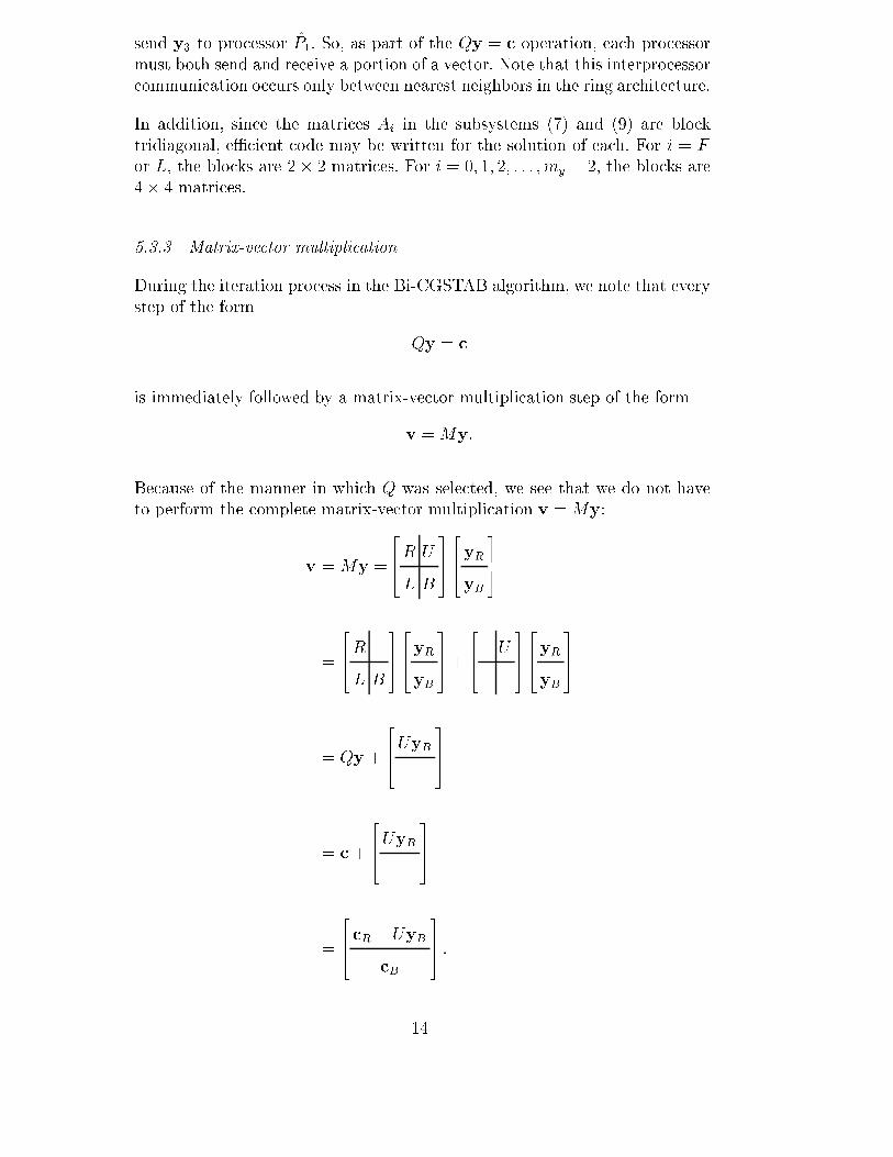
5.3.3 Matrix-vector multiplication

During the iteration process in the Bi-CGSTAB algorithm, we note that everystep of the form

Qy = c

is immediately followed by a matrix-vector multiplication step of the form

v =My.

Because of the manner in which Q was selected, we see that we do not haveto perform the complete matrix-vector multiplication v =My:

v =My =

264R U

L B

375264 yRyB

375

=

264RL B

375264 yRyB

375 +

264 U

375264 yRyB

375

= Qy +

264UyB

375

= c+

264UyB

375

=

264 cR + UyB

cB

375 .

14

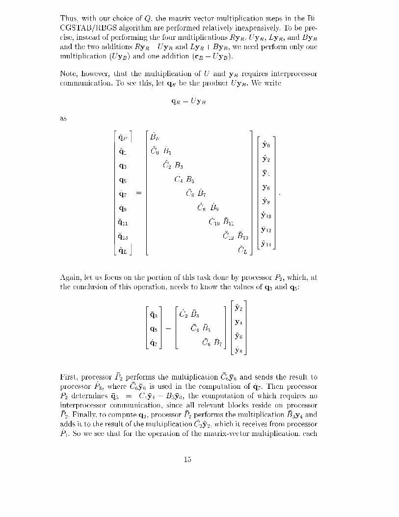
Thus, with our choice of Q, the matrix-vector multiplication steps in the Bi-CGSTAB/RBGS algorithm are performed relatively inexpensively. To be pre-cise, instead of performing the four multiplications RyR, UyB , LyR, and ByBand the two additions RyR+UyB and LyR+ByB, we need perform only onemultiplication (UyB) and one addition (cR + UyB).

Note, however, that the multiplication of U and yB requires interprocessorcommunication. To see this, let qR be the product UyB. We write

qR = UyB

as

2666666666666666666666666664

qF

q1

�q3

�q5

_q7

_q9

�q11

�q13

qL

3777777777777777777777777775

=

2666666666666666666666666664

BF

C0 B1

C2�B3

�C4�B5

�C6_B7

_C8_B9

_C10�B11

�C12�B13

�CL

3777777777777777777777777775

2666666666666666666666664

y0

y2

�y4

�y6

_y8

_y10

�y12

�y14

3777777777777777777777775

.

Again, let us focus on the portion of this task done by processor �P2, which, atthe conclusion of this operation, needs to know the values of �q3 and �q5:

2666664

�q3

�q5

_q7

3777775=

2666664

C2�B3

�C4�B5

�C6_B7

3777775

2666666664

y2

�y4

�y6

_y8

3777777775

First, processor �P2 performs the multiplication �C6�y6 and sends the result toprocessor _P3, where �C6�y6 is used in the computation of _q7. Then processor�P2 determines �q5 = �C4�y4 + �B5�y6, the computation of which requires nointerprocessor communication, since all relevant blocks reside on processor�P2. Finally, to compute �q3, processor �P2 performs the multiplication �B3�y4 andadds it to the result of the multiplication C2y2, which it receives from processorP1. So we see that for the operation of the matrix-vector multiplication, each

15

processor must both send and receive a portion of a vector and that thisinterprocessor communication occurs only between nearest neighbors in thering architecture.

5.4 Implementation on the Cray T3E

We implemented Bi-CGSTAB/RBGS on a Cray T3E, a supercomputer thatcan take advantage of the parallelism inherent in the method. The T3E hasaddress space for 2048 processors con�gured on a three-dimensional torusarchitecture. Further details concerning the technical speci�cations of the T3Emay be found in [25].

We illustrate below that we obtain reasonably good speedups for suÆcientlylarge problem size. We note that the times reported below include only the\main loop" portion of the Bi-CGSTAB/RBGS algorithm which is, of course,where the bulk of the computations occur.

Let TS = serial run time = time required to solve a problem using a singleprocessor. Speci�cally, the algorithm used here is the one-processor versionof the algorithm described above, the code for which does not include anyfeatures speci�c to the T3E or Cray computers in general. In addition, asdiscussed in Section 1, this is the fastest most general serial method known.Let TP = parallel run time = time required to solve a problem using parallelprocessing. Speedup is de�ned as

S = speedup =TS

TP.

Ideally, one would like S = p, a phenomenon known as linear speedup. How-ever, in practice, one observes only sub-linear speedup due to parallel overhead(i.e., manifestations of parallel algorithms that are absent in serial algorithms),the main sources of which are [14]:

� interprocessor communication,

� load imbalance, and

� extra computation.

We saw in our discussion above that interprocessor communication occurs inthree separate operations of the Bi-CGSTAB/RBGS iteration: solving linearsystems of the form Qy = c, matrix-vector multiplication, and in the reduc-tion portion of vector inner product computation. Fortuitously, the interpro-cessor communication is the only signi�cant source contributing to sub-linear

16

speedup. The load is balanced as well as possible (i.e., processors do not sit idlewaiting for messages from other processors before they can resume perform-ing useful computations) and although extra computation does occur, theseredundancies always occur simultaneously across all the processors.

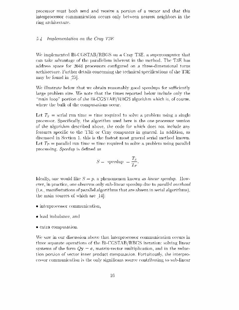
When testing our code on the Cray T3E, we selected a particular PDE withDirichlet boundary conditions and allowed the number of �nite elements inthe x-direction (mx) and the number of �nite elements in the y-direction (my)to (independently) assume the values 16, 32, 64, and 128. We ran the codeusing p = 1, 2, 4, 8, 16, and 32 processors. For each parameter set fmx; my; pg,we ran the code �ve times and then took the mean of these �ve times as therepresentative time used to compile the results given in Table 1.

Table 1Speedup results

mx my p = 1 p = 2 p = 4 p = 8 p = 16 p = 32

16 16 1.0000 1.2106 1.3818

16 32 1.0000 1.3881 1.8314 2.1219

16 64 1.0000 1.6372 2.2701 3.1482 3.7461

16 128 1.0000 1.7782 2.8277 4.3781 5.5691 6.4388

32 16 1.0000 1.4578 1.8974

32 32 1.0000 1.5980 2.3621 3.0986

32 64 1.0000 1.6408 2.7593 4.4253 5.5811

32 128 1.0000 1.8731 3.3643 5.6086 8.4241 11.3382

64 16 1.0000 1.5828 2.3070

64 32 1.0000 1.7641 2.9244 4.2942

64 64 1.0000 1.8707 3.4074 5.6325 8.2351

64 128 1.0000 1.9059 3.3788 6.5883 10.1703 16.1655

128 16 1.0000 1.7507 2.8698

128 32 1.0000 1.8780 3.4103 5.6460

128 64 1.0000 1.9383 3.6523 6.6972 11.1015

128 128 1.0000 1.9717 3.8835 7.3626 12.8075 22.0124

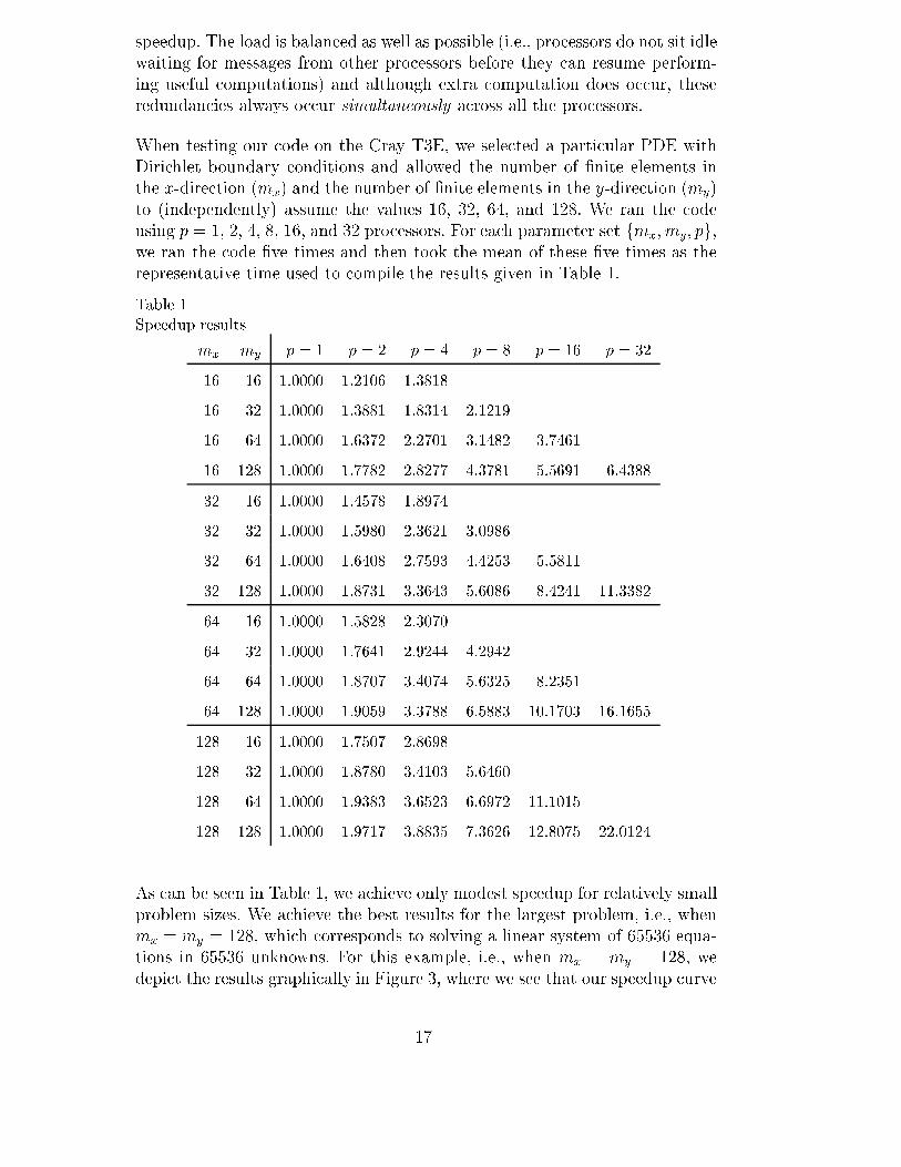
As can be seen in Table 1, we achieve only modest speedup for relatively smallproblem sizes. We achieve the best results for the largest problem, i.e., whenmx = my = 128, which corresponds to solving a linear system of 65536 equa-tions in 65536 unknowns. For this example, i.e., when mx = my = 128, wedepict the results graphically in Figure 3, where we see that our speedup curve

17

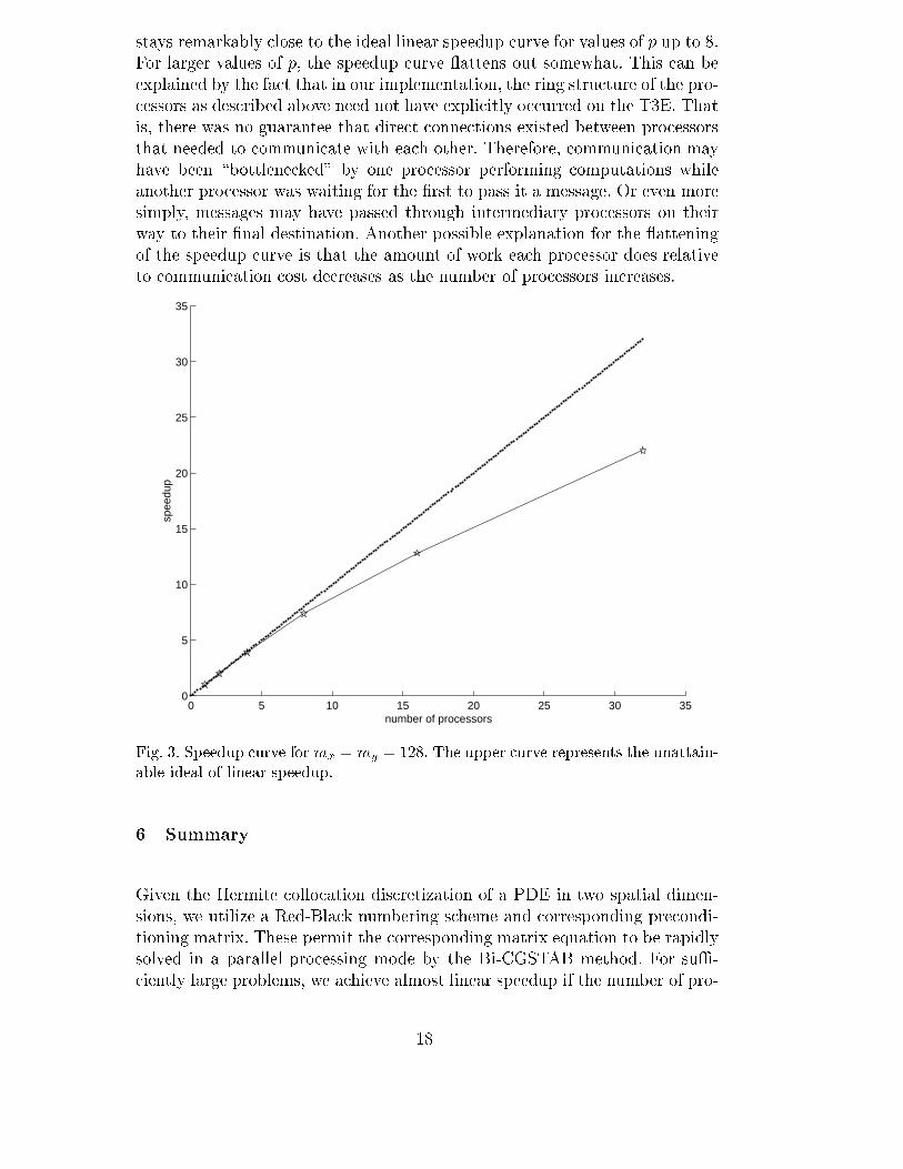
stays remarkably close to the ideal linear speedup curve for values of p up to 8.For larger values of p, the speedup curve attens out somewhat. This can beexplained by the fact that in our implementation, the ring structure of the pro-cessors as described above need not have explicitly occurred on the T3E. Thatis, there was no guarantee that direct connections existed between processorsthat needed to communicate with each other. Therefore, communication mayhave been \bottlenecked" by one processor performing computations whileanother processor was waiting for the �rst to pass it a message. Or even moresimply, messages may have passed through intermediary processors on theirway to their �nal destination. Another possible explanation for the atteningof the speedup curve is that the amount of work each processor does relativeto communication cost decreases as the number of processors increases.

0 5 10 15 20 25 30 350

5

10

15

20

25

30

35

number of processors

spee

dup

Fig. 3. Speedup curve formx = my = 128. The upper curve represents the unattain-able ideal of linear speedup.

6 Summary

Given the Hermite collocation discretization of a PDE in two spatial dimen-sions, we utilize a Red-Black numbering scheme and corresponding precondi-tioning matrix. These permit the corresponding matrix equation to be rapidlysolved in a parallel processing mode by the Bi-CGSTAB method. For suÆ-ciently large problems, we achieve almost linear speedup if the number of pro-

18

cessors is 8 or less. When a greater number of processors is used, the speedupcurve attens out somewhat. We believe that this could be ameliorated byensuring that the ring architecture favored by our method be embedded uponthe architecture of the parallel processing computer being used.

Acknowledgments

The authors gratefully acknowledge the contribution of Dr. Ilene Carpenter ofCray Research/SGI, for providing access to the T3E supercomputer and forher magnanimous assistance during the numerical experiments. We also thankthe referees for their insightful comments and suggestions.

References

[1] B. Bialecki, G. Fairweather, and K. R. Bennett, Fast Direct Solvers for PiecewiseHermite Bicubic Orthogonal Spline Collocation Equations, SIAM J. Numer.

Anal. 29 (1992) 156{173.

[2] S. H. Brill, Hermite Collocation Solution of Partial Di�erential Equations viaPreconditioned Krylov Methods, Numerical Methods for Partial Di�erential

Equations 17 (2001) 120{136.

[3] S. H. Brill, Documentation for Collocation Software, RCGRD Publication#98-01, Research Center for Groundwater Remediation Design, University ofVermont, Burlington, Vermont, 1998. Available at the World Wide Web sitehttp://math.boisestate.edu/~brill/research/doc coll.html.

[4] S. H. Brill and G. F. Pinder, Analysis of a Block Red-Black PreconditionerApplied to the Hermite Collocation Discretization of a Model ParabolicEquation, Numerical Methods for Partial Di�erential Equations, in press.

[5] S. H. Brill and G. F. Pinder, Eigenvalue Analysis of a Block Red-Black Gauss-Seidel Preconditioner Applied to the Hermite Collocation Discretization ofPoisson's Equation, Numerical Methods for Partial Di�erential Equations 17

(2001) 204{228.

[6] S. H. Brill and G. F. Pinder, A Parallel Preconditioned Bi-ConjugateGradient Algorithm for Two-Dimensional Elliptic and Parabolic EquationsUsing Hermite Collocation, Proceedings of the Eighth SIAM Conference on

Parallel Processing for Scienti�c Computing (1997).

[7] P. Chin and P. A. Forsyth, A Comparison of GMRES andCGSTAB Accelerations for Incompressible Navier-Stokes Problems, Journal ofComputational and Applied Mathematics 46 (1993) 415{426.

19

[8] C. C. Christara, Quadratic Spline Collocation Methods for Elliptic PartialDi�erential Equations, BIT 34 (1998) 33{61.

[9] C. C. Christara, E. N. Houstis, and J. R. Rice, A Parallel Spline Collocation-Capacitance Method for Elliptic Partial Di�erential Equations, SupercomputingConference Proceedings (1988) 375{384.

[10] R. D. da Cunha and T. Hopkins, Parallel Iterative Methods. Available at theWorld Wide Web site http://www.mat.ufrgs.br/~rudnei/pim/pim-i.html.

[11] E. O. Frind and G. F. Pinder, A Collocation Finite Element Method forPotential Problems in Irregular Domains, Int. J. Numer. Meth. Eng. 14 (1979)681{701.

[12] J. F. Guarnaccia and G. F. Pinder, A Collocation Based Parallel Algorithm toSolve Immiscible Two Phase Flow in Porous Media, Proceedings of the Fifth

SIAM Conference on Parallel Processing for Scienti�c Computing , (1992) 205{210.

[13] C. E. Houstis, E. N. Houstis, and J. R. Rice, Partitioning PDE Computations:Methods and Performance Evaluation, Parallel Computing 5 (1987) 141{163.

[14] V. Kumar, A. Grama, A. Gupta, and G. Karypis, Introduction to Parallel

Computing (Benjamin/Cummings Publishing Company, Inc., Redwood City,California, 1994).

[15] C.-C. J. Kuo and T. F. Chan, Two-Color Fourier Analysis of IterativeAlgorithms for Elliptic Problems with Red/Black Ordering, SIAM J. Sci. Stat.

Comput. 11 (1990) 767{793.

[16] Y.-L. Lai, A. Hadjidimos, E. N. Houstis, and J. R. Rice, On the IterativeSolution of Hermite Collocation Equations, SIAM J. Matrix Anal. Appl. 16

(1995) 254{277.

[17] T. S. Papatheodorou, Block AOR Iteration for Nonsymmetric Matrices, Math.

Comp. 41 (1983), 511{525.

[18] T. S. Papatheodorou and Y. G. Saridakis, Parallel Algorithms and Architecturesfor Multisplitting Iterative Methods, Parallel Computing 12 (1989) 171{182.

[19] P. M. Prenter and R. D. Russell, Orthogonal Collocation for Elliptic PartialDi�erential Equations, SIAM J. Numer. Anal. 13 (1976) 923{939.

[20] Y. Saad and M. H. Schultz, GMRES: A Generalized Minimal ResidualAlgorithm for Solving Nonsymmetric Linear Systems, SIAM J. Sci. Stat.

Comput. 7 (1986) 856{869.

[21] W. Schmid, M. Pa�rath, and R. H. W. Hoppe, Application of Iterative Methodsfor Solving Nonsymmetric Linear Systems in the Simulation of SemiconductorProcessing, Surveys on Mathematics for Industry 5 (1995) 1{26.

[22] H. A. van der Vorst, Bi-CGSTAB: A Fast and Smoothly Converging Variant ofBi-CG for the Solution of Nonsymmetric Linear Systems, SIAM J. Sci. Stat.

Comput. 13 (1992) 631{644.

20

[23] C. Vulk, Further Experiences with GMRESR, Supercomputer 10 (1993) 13{27.

[24] World Wide Web site:http://www.math.boisestate.edu/~brill/research/cray code.html.

[25] World Wide Web site:http://www.tera.com//products/systems/crayt3e/paper1.html.

21