string field theory and its applications
TRANSCRIPT

String Field Theory and its Applications
Ashoke Sen
Harish-Chandra Research Institute, Allahabad, India
Florence, April 2019
1

What is string fieldtheory?
2

In the conventional world-sheet approach to string theory, thescattering amplitudes with n external states take the form:∑
g≥0
(gs)2g∫
Mg,n
Ig,n
Mg,n: Moduli space of genus g Riemann surface with n punctures
Ig,n: an appropriate correlation function of vertex operators andother operators (ghosts, PCOs) on a genus g Riemann surface.
3

String field theory is a quantum field theory with infinite numberof fields in which perturbative amplitudes are computed bysumming over Feynman diagrams.
Each Feynman diagram can be formally represented as anintegral over the moduli space of a Riemann surface with
– the correct integrand Ig,n (as in world-sheet description)
– but only a limited range of integration.
Sum over all Feynman diagrams reproduces the integration overthe whole moduli space Mg,n.
4
Why should we study string field theory?
Original motivation: Use string field theory to give anon-perturbative definition of string theory.
In this talk the focus will be to use string field theory to betterunderstand string perturbation theory
– address the ‘infra-red issues’ to make perturbation theorywell-defined.
In the rest of the talk we shall focus on closed string fieldtheories.
Review: arXiv:1703.06410Corinne de Lacroix, Harold Erbin, Sitender Pratap Kashyap, A.S., Mritunjay Verma
5

General structure ofstring field theory
6

Begin with classical closed bosonic string field theorySaadi, Zwiebach; Kugo, Suehiro; Sonoda, Zwiebach; Zwiebach; · · ·
A string field ψ is an element of some vector space H.
H is a subspace of the full Hilbert space of matter and ghostworld-sheet CFT, defined by the constraints:
b−0 |ψ〉 = 0, L−0 |ψ〉 = 0, ng|ψ〉 = 2|ψ〉
b±0 = b0 ± b̄0, L±0 = L0 ± L̄0, c±0 =12
(c0 ± c̄0)
ng = ghost number
Matter CFT: Any CFT with c=26.
Note: No physical state constraint on |ψ〉
7

If {|φr〉} is a basis in H, then we can expand |ψ〉 as
|ψ〉 =∑
r
ψr|φr〉
ψr are the dynamical degrees of freedom
– path integral ≡ integration over the ψr ’s
∑r includes integration over momenta along non-compact
directions
⇒ makes ψr into fields (in momentum space)
8

Classical action (setting gs = 1):
S =12〈ψ|c−0 QB|ψ〉+
∑n
1n!{ψn}
QB: BRST charge
For |Ai〉 ∈ H, {A1 · · ·An} is constructed from correlationfunctions of the vertex operators Ai on the sphere, integratedover a subspace S of the moduli space M0,n.
1. Since Ai’s are off-shell, the correlation function depends onthe choice of world-sheet metric, or equivalently the choice oflocal coordinate system z in which the metric = |dz|2 locally.
2. The subspace S avoids all degenerations, and its choice iscorrelated with the choice of local coordinates in step 1.
Different choices (z, S) give equivalent string field theoriesrelated by field redefinition
9

S =12〈ψ|c−0 QB|ψ〉+
∑n
1n!{ψn}
This action has infinite parameter gauge invariance of the form
δ|ψ〉 = QB|λ〉+ · · ·
|λ〉 represents gauge transformation parameter.
This theory can be quantized using Batalin-Vilkovisky (BV)formalism
– introduces ghosts and anti-fields
10

Net result: Relax the constraint on the ghost number of |ψ〉.
The action has similar structure:
SBV =12〈ψ|c−0 QB|ψ〉+
∑n
1n!{ψn}
But now {A1 · · ·An} contains contribution from integrals oversubspaces of Mg,n for all g
The higher genus contributions are needed to cancel gaugenon-invariance of the path integral measure.
Note: We shall continue to use the symbols
H for this extended Hilbert space carrying arbitrary ng
|ψ〉 for the extended string field ∈ H
{A1 · · ·An} for the new, quantum corrected product.
11
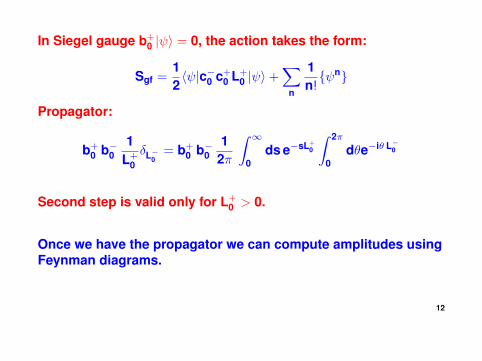
In Siegel gauge b+0 |ψ〉 = 0, the action takes the form:
Sgf =12〈ψ|c−0 c+
0 L+0 |ψ〉+
∑n
1n!{ψn}
Propagator:
b+0 b−0
1L+
0δL−0
= b+0 b−0
12π
∫ ∞0
ds e−sL+0
∫ 2π
0dθe−iθ L−0
Second step is valid only for L+0 > 0.
Once we have the propagator we can compute amplitudes usingFeynman diagrams.
12
Each Feynman diagram has vertices and propagators.
We have some integrals from the vertices (integration oversubspaces of Mg′,n′ ).
g′,n′ refer to individual vertices
We also have two integrals from each propagator (s, θ)
Together the total set of integrals can be interpreted as integralover a subspace of Mg,n with the correct integrand
(g,n) refer to the full amplitude
Sum over all Feynman diagrams generate integration over thefull moduli space Mg,n with the correct integrand
13

Instead of summing over all Feynman diagrams, one could sumover only one particle irreducible (1PI) diagrams
– gives 1PI effective action
S1PI =12〈ψ|c−0 QB|ψ〉+
∑n
1n!{ψn}1PI
The definition of {A1 · · ·An}1PI remains similar to that of{A1 · · ·An}, except that the subspace of Mg,n that we integrateover is larger
– includes boundaries of the moduli space that arenon-separating type
(degenerating cycle that does not split the Riemann surface intotwo disconnected parts.)
14

Separating Non-separating
Note: For bosonic string theory, the 1PI effective action is aformal object due to tachyons propagating in the loop.
But there will be no such problem in heterotic and type IItheories.
15
Heterotic string theory:
World-sheet theory contains β, γ ghosts and associated ξ, η, φsystem after bosonization
β = ∂ξ e−φ, γ = η eφ
Hilbert space H splits into direct sum ⊕nHn
n: picture number
– integer for NS sector, integer + 1/2 for R sector
Picture changing operator (PCO) Friedan, Martinec, Shenker; Knizhnik
X (z) = {QB, ξ(z)}
16
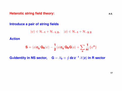
Heterotic string field theory: A.S.
Introduce a pair of string fields
|ψ〉 ∈ H−1 +H−1/2, |φ〉 ∈ H−1 +H−3/2
Action
S = 〈φ|c−0 QB|ψ〉 −12〈φ|c−0 QBG|φ〉+
∑n
1n!{ψn}
G=Identity in NS sector, G = X0 ≡∮
dz z−1 X (z) in R sector
17
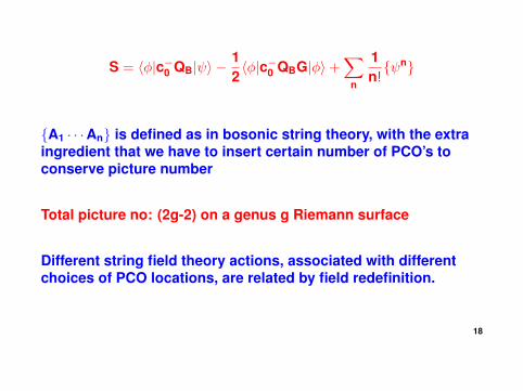
S = 〈φ|c−0 QB|ψ〉 −12〈φ|c−0 QBG|φ〉+
∑n
1n!{ψn}
{A1 · · ·An} is defined as in bosonic string theory, with the extraingredient that we have to insert certain number of PCO’s toconserve picture number
Total picture no: (2g-2) on a genus g Riemann surface
Different string field theory actions, associated with differentchoices of PCO locations, are related by field redefinition.
18

〈φ|c−0 QB|ψ〉 −12〈φ|c−0 QBG|φ〉+
∑n
1n!{ψn}
Note: We have doubled the number of degrees of freedom (|φ〉and |ψ〉)
However since |φ〉 enters the action at most quadratically, itdescribes free field degrees of freedom
– completely decouples from the interacting part of the theorydescribed by |ψ〉
– has no observable effects.
Quantization of this theory proceeds in the same way as inbosonic string theory.
19

For type II string theory the structure of the theory is similar.
|ψ〉 ∈ H−1,−1 ⊕H−1,−1/2 ⊕H−1/2,−1 ⊕H−1/2,−1/2
|φ〉 ∈ H−1,−1 ⊕H−1,−3/2 ⊕H−3/2,−1 ⊕H−3/2,−3/2
S = 〈φ|c−0 QB|ψ〉 −12〈φ|c−0 QBG|φ〉+
∑n
1n!{ψn}
G: identity in NSNS sector, X0 in NSR sector,
X̄0 in RNS sector, X0X̄0 in RR sector
20
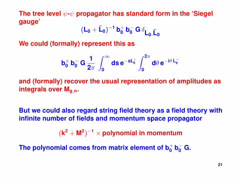
The tree level ψ-ψ propagator has standard form in the ‘Siegelgauge’
(L0 + L̄0)−1 b+0 b−0 G δL0,L̄0
We could (formally) represent this as
b+0 b−0 G
12π
∫ ∞0
ds e−sL+0
∫ 2π
0dθ e−iθ L−0
and (formally) recover the usual representation of amplitudes asintegrals over Mg,n.
But we could also regard string field theory as a field theory withinfinite number of fields and momentum space propagator
(k2 + M2)−1 × polynomial in momentum
The polynomial comes from matrix element of b+0 b−0 G.
21

k1 k2
k3kn · · ·
Vertices are accompanied by a suppression factor of
exp
[−A
2
∑i
(k2i + m2
i )
]
A: a positive constant whose precise value depends on thechoice of coordinate system used to define the off-shell vertex.
Hata, Zwiebach
This makes
– momentum integrals UV finite (almost)
– sum over intermediate states converge22

Momentum dependence of vertex includes
exp
[−A
2
∑i
(k2i + m2
i )
]= exp
[−A
2
∑i
(~k2
i + m2i ) +
A2
(k0i )2
]
Integration over ~ki converges for large |~ki|, but integration overk0
i diverges at large |k0i |.
The spatial components of loop momenta can be integratedalong the real axis, but we have to treat integration over loopenergies more carefully.
23

Resolution: Need to have the ends of loop energy integralsapproach ±i∞.
In the interior the contour may have to be deformed away fromthe imaginary axis to avoid poles from the propagators.
Complex k0-plane
××
We shall now describe how to choose the loop energyintegration contour.
24

General procedure: Pius, A.S.
1. Begin with a configuration of off-shell external momentawhere all energies are imaginary and all spatial momenta arereal.
2. In this case we can take all loop energy contours to lie alongthe imaginary axis without encountering any singularity.
3. Now deform the energies to real values (Wick rotation)
4. If some pole of a propagator approaches the loop energyintegration contours, deform the contours away from the pole,keeping their ends at ±i∞.
Result: Such deformations are always possible
– the loop energy contours do not get pinched by poles from twosides during this deformation.
25

Applications
26

Momentum space integrals vs integrals over Mg,n:
Key link:
1L+
0δL−0
=1
2π
∫ ∞0
ds e−sL+0
∫ 2π
0dθ e−iθ L−0
1. For L+0 < 0 the left hand side is finite but the right hand side is
divergent (as s→∞)
2. For L+0 = 0 both sides are divergent.
All divergences appearing in the world-sheet description havetheir origin in one of these two cases.
– divergences appearing at the boundary of Mg,n where theRiemann surface degenerates
27

1L+
0δL−0
=1
2π
∫ ∞0
ds e−sL+0
∫ 2π
0dθ e−iθ L−0
For L+0 < 0 the left hand side is finite
⇒ string field theory gives perfectly finite result even thoughintegral over Mg,n diverges
For L+0 = 0 both sides are divergent
But in string field theory these are associated with some internalpropagator going on-shell
⇒ field theory intuition tells us how to handle them
28
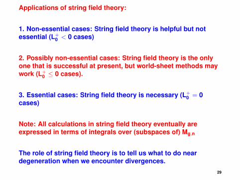
Applications of string field theory:
1. Non-essential cases: String field theory is helpful but notessential (L+
0 < 0 cases)
2. Possibly non-essential cases: String field theory is the onlyone that is successful at present, but world-sheet methods maywork (L+
0 ≤ 0 cases).
3. Essential cases: String field theory is necessary (L+0 = 0
cases)
Note: All calculations in string field theory eventually areexpressed in terms of integrals over (subspaces of) Mg,n
The role of string field theory is to tell us what to do neardegeneration when we encounter divergences.
29

Example of a non-essential case:
Consider N tachyon amplitude in bosonic string theory
∝∫ N∏
i=4
d2zi
∏i<j
|zi − zj|pi.pj
This integral diverges if pi.pj < −2 for any pair (i,j).
– needs to be defined via analytic continuation.
Not very useful for numerical evaluation.
Witten’s iε prescription treats Re(ln zi) and Im(ln zi) as complexvariables and turns the Re(ln zi) contours into complex plane.
Makes divergent integrals into oscillatory integrals, but we stillneed to apply some numerical trick to evaluate the integrals.
30

In string field theory these divergences can be associated withL+
0 < 0 states propagating in the internal line.
We need to represent the propagator by 1/L+0 instead of using
Schwinger parametrization.
This suggests a specific procedure.
1. Remove all regions where 2 or more zi’s approach each other
– gives a finite integral.
2. The missing regions are compensated for by adding boundaryterms.
Also need additional boundary terms where two boundariesintersect etc.
The boundary terms correspond to Feynman diagrams with oneor more internal propagators.
The bulk term corresponds to the elementary N-string vertex. 31
Examples of possibly non-essential cases:
1. Proof of unitarity
2. Finding the domain of analyticity of the S-matrix
32

Unitarity: Mercus; Amano, Tsuchiya; Sundborg; Berera; D’Hoker, Phong; Iengo, Russo; Witten
String theory amplitudes, written as integrals over Mg,n, arealways formally hermitian (T− T† = 0)
– apparently violates unitarity
However one finds by examining the integrals over Mg,n that theintegrals diverge whenever the external momenta go above thethreshold of production of intermediate states
– related to the fact that some particle propagating in the loophas L+
0 < 0.
Therefore the apparent reality is only formal, and one has todefine the integral by analytic continuation.
33

Witten’s iε prescription gives a way to define these integrals in away that makes them manifestly finite but complex.
But to construct a direct proof that the amplitudes defined thisway satisfy the Cutkosky rules is hard.
String field theory can be used to solve this problem. Pius, A.S.
Since string field theory defines the loop amplitudes asmomentum integrals in complex momentum space, itautomatically comes with some ‘iε prescription’.
1. One can give a direct proof of Cutkosky rules using Feynmandiagram analysis.
2. One can show that this agrees with Witten’s iε prescription.
34
Domain of analyticity:
Consider a general amplitude characterized by a set ofMandelstam variables:
sij = −(pi + pj)2
In which domain in the complex sij plane is the S-matrixanalytic?
– related to the question of crossing symmetry (ability toanalytically continue from one physical channel to another)
– believed to be related to the question of locality
35

In principle this question can be addressed without goingoff-shell but at present this seems to be hard.
The generalization of Witten’s iε prescription for complexexternal momenta is not known yet.
36

String field theory allows us to use an old approach in(axiomatic) quantum field theory.
Jost, Lehmann; Dyson; Bros, Messiah, Stora; Bros, Epstein, Glaser
1. Use the locality of the position space Green’s function toprove analyticity of the off-shell momentum space Green’sfunctions in certain primitive domain.
2. Then extend the domain using general properties of functionsof many complex variables.
3. Study the intersection of this domain with the mass-shell.
This has been generalized to string field theory. de Lacroix, Erbin, A.S.
Non-trivial step is step 1 since we do not have analog of positionspace Green’s function on which we impose locality.
Instead we analyze momentum space Feynman diagramsdirectly to find the primitive domain. 37

Examples of essential cases: Pius, Rudra, A.S.; A.S.
1. Vacuum shift
2. Mass renormalization
38

For a given amplitude, the usual world-sheet description ofstring perturbation theory gives one term at every loop order
– usually considered an advantage, but this may not always bethe case
e.g. in a quantum field theory, self energy insertions on externallegs need special treatment.
ll lSteps required:
1. Separate graphs with self-energy insertions on external lines
2. Resum to compute off-shell 2-point function
3. Look for pole positions39

In the usual world-sheet approach we do not do any of this.
Result: integration over Mg,n diverges from the separating typedegeneration.
××
××
40
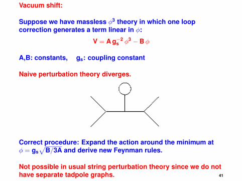
Vacuum shift:
Suppose we have massless φ3 theory in which one loopcorrection generates a term linear in φ:
V = A g−2s φ3 − Bφ
A,B: constants, gs: coupling constant
Naive perturbation theory diverges.
Correct procedure: Expand the action around the minimum atφ = gs
√B/3A and derive new Feynman rules.
Not possible in usual string perturbation theory since we do nothave separate tadpole graphs. 41

Result: Tadpole divergence in integration over Mg,n.
×
××
In contrast, in string field theory we can deal with massrenormalization and vacuum shift by following the standardprocedure in quantum field theory.
42

Vacuum shift and mass renormalization in string field theory
Step 1. Construct the 1PI effective action
{A1 · · ·AN}1PI: 1PI amplitude of states A1, · · · ,AN computed fromthe string field theory
{A1 · · ·AN}1PI =∑
g
(gS)2g∫Rg,N
〈· · ·A1 · · ·AN〉g,N
Rg,N: a subspace of Mg,N corresponding to sum of 1PI diagrams
S1PI =1
g2S
[−1
2〈φ|c−0 QB G|φ〉+ 〈φ|c−0 QB|ψ〉+
∞∑N=1
1N!{ψN}1PI
]
43

Step 2: Derive equations of motion from S1PI
QB(G|φ〉 − |ψ〉) = 0
QB|φ〉+∞∑
N=0
1N!
[ψN] = 0
[A1 · · ·AN] ∈ H is defined via:
〈A|c−0 [A1 · · ·AN]〉 = {A A1 · · ·AN}1PI
Combine two equations to get the interacting field equation:
QB|ψ〉+∞∑
N=0
1N!
G [ψN] = 0
Systematically construct the vacuum solution in the zeromomentum sector in power series in gs:
QB|ψv〉+∞∑
N=0
1N!
G [ψNv ] = 0
44

Step 3. Define|χ〉 = |ψ〉 − |ψv〉
and expand the action in powers of |χ〉 to derive new Feynmanrules.
For mass renormalization, analyze linearized equations ofmotion of |χ〉 in the background |ψv〉.
Result:
QB|χ〉+∞∑
N=0
1N!
G [ψNv χ] = 0
Solve this equation systematically in a power series in gs
If the solution exists at p2 + M2 = 0 then M is the renormalizedmass.
Solutions which exist for all p are pure gauge 45

Details of the iterative construction of the vacuum solution:
Suppose |ψk〉 is the solution to order gsk. (|ψ0〉 = 0)
P: projection operator to L+0 ≡ L0+L̄0 = 0 states.
Then
|ψk+1〉 = −b+
0
L+0
k+1∑N=0
1N!
(1− P) G [ψNk ] + |ξk+1〉 ,
|ξk+1〉 is an L+0 = 0 state satisfying
QB|ξk+1〉 = −k+1∑N=0
1N!
P G [ψNk ] +O(gs
k+2) .
46
|ψk+1〉 = −b+
0
L+0
k+1∑N=0
1N!
(1− P) G [ψNk ] + |ξk+1〉 ,
QB|ξk+1〉 = −k+1∑N=0
1N!
P G [ψNk ] +O(gs
k+2) .
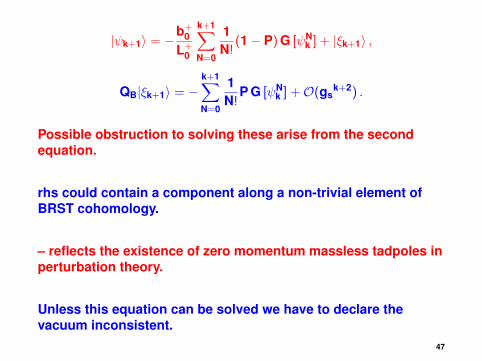
Possible obstruction to solving these arise from the secondequation.
rhs could contain a component along a non-trivial element ofBRST cohomology.
– reflects the existence of zero momentum massless tadpoles inperturbation theory.
Unless this equation can be solved we have to declare thevacuum inconsistent.
47

|ψk+1〉 = −b+
0
L+0
k+1∑N=0
1N!
(1− P) G [ψNk ] + |ξk+1〉 ,
QB|ξk+1〉 = −k+1∑N=0
1N!
P G [ψNk ] +O(gs
k+2) .
Once these equations have been solved, we do not encounterany further tadpole divergence in perturbation theory.
Note: The full solution |ψv〉 is |ψ∞〉, but in practice we shall stopat some fixed order in gs.
Similar iterative procedure can be used to solve linearizedequations for fluctuations around the vacuum and hence therenormalized masses.
48

This also allows us to deal with the cases involving multiplesolutions, e.g. when a scalar field χ in low energy theory haspotential
c g−2s (χ2 − K gs
2)2 .
At order gs we have three solutions χ = 0,±gs√
K.
In 1PI effective string field theory this will be reflected in theexistence of multiple solutions for |ψ1〉.
The solution corresponding to χ = 0 will have non-zero dilatonone point function at higher order
⇒ an obstruction to extending the corresponding 1PI effectivefield theory solution to higher order.
The solutions corresponding to χ = ±gs√
K will not encountersuch obstructions.
49
This situation arises in SO(32) heterotic string compactificationon Calabi-Yau manifolds.
String field theory analysis reproduces all the results expectedfrom supersymmetry.
1. Existence of multiple solutions at low order.
2. Correct one loop renormalized scalar and fermion masses,both at the maximum and the minimum of the potential.
3. Correct value of two loop dilaton tadpole at the maximum.
4. Vanishing dilaton tadpole at the minimum.
50

Similar iterative approach can also be used to constructsolutions in string field theory corresponding to marginaldeformations by NSNS or RR fields. Cho, Collier, Yin
51

Practical difficulties in pushing this to higher order:
Construction of 1PI effective action requires choosing localcoordinates on the world-sheet and PCO locations to define the1PI vertices.
It is hard to find an explicit systematic procedure for makingthese choices.
Final result is known to be independent of these choices but wehave to make these choices to do computation
Once a systematic procedure for making these choices is foundthen one could make this into an automated procedure.
52

So far there are two concrete proposals based on minimal areametric and constant negative curvature metric.
Zwiebach; Moosavian, Pius
Requires more effort to make them into useful computationaltools.
Alternative approach: Try to develop a formalism where theindependence of physical quantities on the choice of localcoordinates and PCO locations is manifest all through thecomputation.
53
Conclusion
String field theory was originally designed to studynon-perturbative aspects of string theory.
However it is also a useful tool for making perturbation theorywell defined.
When the world-sheet approach works fine, we do not needstring field theory.
When in doubt, we can invoke string field theory.
54