supervised learning. introduction 3 why “learn”? machine learning is programming computers to...

Supervised Learning

Introduction

3

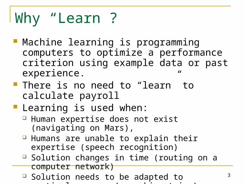
Why “Learn”? Machine learning is programming computers to

optimize a performance criterion using example data or past experience.

There is no need to “learn” to calculate payroll Learning is used when:

Human expertise does not exist (navigating on Mars), Humans are unable to explain their expertise (speech

recognition) Solution changes in time (routing on a computer

network) Solution needs to be adapted to particular cases (user

biometrics)

4

What We Talk About When We Talk About“Learning”

Learning general models from a data of particular examples

Data is cheap and abundant (data warehouses, data marts); knowledge is expensive and scarce.

Example in retail: Customer transactions to consumer behavior:

People who bought “Da Vinci Code” also bought “The Five People You Meet in Heaven” (www.amazon.com)

Build a model that is a good and useful approximation to the data.

5

What is Machine Learning? Study of algorithms that improve their

performance at some task with experience Optimize a performance criterion using example

data or past experience. Role of Statistics: Inference from a sample Role of Computer science: Efficient algorithms to

Solve the optimization problem Representing and evaluating the model for inference

Growth of Machine Learning Machine learning is preferred approach to

Speech recognition, Natural language processing Computer vision Medical outcomes analysis Robot control Computational biology

This trend is accelerating

Improved machine learning algorithms Improved data capture, networking, faster computers Software too complex to write by hand New sensors / IO devices Demand for self-customization to user, environment It turns out to be difficult to extract knowledge from human

expertsfailure of expert systems in the 1980’s.

Alpydin & Ch. Eick: ML Topic1 6

7

Applications

Association Analysis Supervised Learning

Classification Regression/Prediction

Unsupervised Learning Reinforcement Learning

Learning Associations Basket analysis:

P (Y | X ) probability that somebody who buys X also buys Y where X and Y are products/services.

Example: P ( chips | beer ) = 0.7 Market-Basket transactions

TID Items

1 Bread, Milk

2 Bread, Diaper, Beer, Eggs

3 Milk, Diaper, Beer, Coke

4 Bread, Milk, Diaper, Beer

5 Bread, Milk, Diaper, Coke

9

Classification Example: Credit

scoring Differentiating

between low-risk and high-risk customers from their income and savings

Discriminant: IF income > θ1 AND savings > θ2 THEN low-risk ELSE high-risk

Model

10

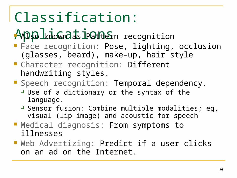
Classification: Applications Also known as Pattern recognition Face recognition: Pose, lighting, occlusion

(glasses, beard), make-up, hair style Character recognition: Different handwriting

styles. Speech recognition: Temporal dependency.

Use of a dictionary or the syntax of the language. Sensor fusion: Combine multiple modalities; eg,

visual (lip image) and acoustic for speech Medical diagnosis: From symptoms to illnesses Web Advertizing: Predict if a user clicks on an

ad on the Internet.

11

Face Recognition

Training examples of a person

Test images

AT&T Laboratories, Cambridge UK http://www.uk.research.att.com/facedatabase.html

12

Prediction: Regression

Example: Price of a used car

x : car attributes

y : price

y = g (x | θ )

g ( ) : model,

θ : parameters

y = wx+w0

13

Regression Applications

Navigating a car: Angle of the steering wheel (CMU NavLab)

Kinematics of a robot armα1= g1(x,y)

α2= g2(x,y)

α1

α2

(x,y)

14

Supervised Learning: Uses

Prediction of future cases: Use the rule to predict the output for future inputs

Knowledge extraction: The rule is easy to understand

Compression: The rule is simpler than the data it explains

Outlier detection: Exceptions that are not covered by the rule, e.g., fraud

Example: decision trees tools that create rules

15

Unsupervised Learning

Learning “what normally happens” No output Clustering: Grouping similar instances Other applications: Summarization,

Association Analysis Example applications

Customer segmentation in CRM Image compression: Color quantization Bioinformatics: Learning motifs

16

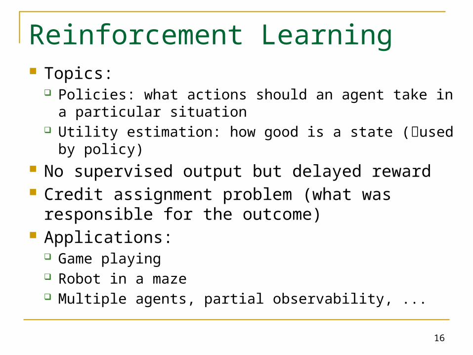
Reinforcement Learning Topics:

Policies: what actions should an agent take in a particular situation

Utility estimation: how good is a state (used by policy) No supervised output but delayed reward Credit assignment problem (what was responsible

for the outcome) Applications:

Game playing Robot in a maze Multiple agents, partial observability, ...

17

Road Map Basic concepts Decision tree induction Evaluation of classifiers Rule induction Classification using association rules Naïve Bayesian classification Naïve Bayes for text classification Support vector machines K-nearest neighbor Summary

18

An example application

An emergency room in a hospital measures 17 variables (e.g., blood pressure, age, etc) of newly admitted patients.

A decision is needed: whether to put a new patient in an intensive-care unit.

Due to the high cost of ICU, those patients who may survive less than a month are given higher priority.

Problem: to predict high-risk patients and discriminate them from low-risk patients.

19

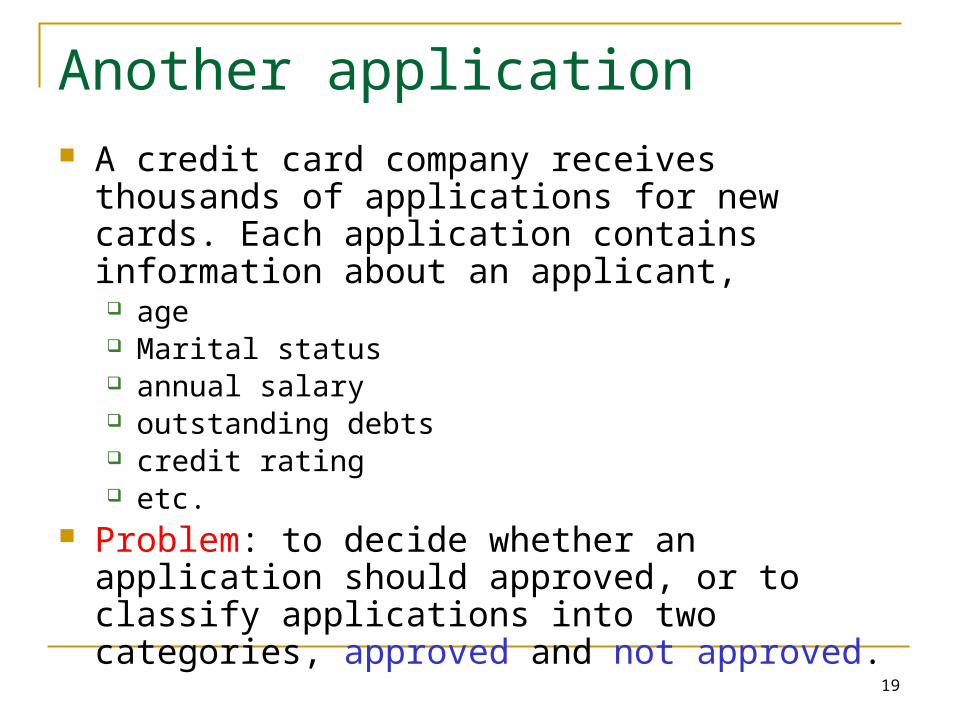
Another application A credit card company receives thousands of

applications for new cards. Each application contains information about an applicant, age Marital status annual salary outstanding debts credit rating etc.

Problem: to decide whether an application should approved, or to classify applications into two categories, approved and not approved.

20

Machine learning and our focus Like human learning from past experiences. A computer does not have “experiences”. A computer system learns from data, which

represent some “past experiences” of an application domain.

Our focus: learn a target function that can be used to predict the values of a discrete class attribute, e.g., approve or not-approved, and high-risk or low risk.

The task is commonly called: Supervised learning, classification, or inductive learning.

21

Data: A set of data records (also called examples, instances or cases) described by k attributes: A1, A2, … Ak. a class: Each example is labelled with a pre-

defined class. Goal: To learn a classification model from the

data that can be used to predict the classes of new (future, or test) cases/instances.

The data and the goal

22

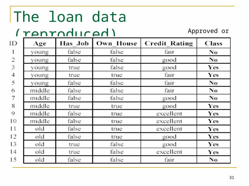
An example: data (loan application) Approved or not

23

An example: the learning task1) Learn a classification model from the data

2) Use the model to classify futureloan applications into

Yes (approved) and No (not approved)

What is the class for following case/instance?

24

Supervised vs. unsupervised Learning Supervised learning: classification is seen as

supervised learning from examples. Supervision: The data (observations,

measurements, etc.) are labeled with pre-defined classes. It is like that a “teacher” gives the classes (supervision).

Test data are classified into these classes too. Unsupervised learning (clustering)

Class labels of the data are unknown Given a set of data, the task is to establish the

existence of classes or clusters in the data

25

Supervised learning process: two steps1. Learning (training): Learn a model using the

training data2. Testing: Test the model using unseen test

data to assess the model accuracy

,cases test ofnumber Total

tionsclassificacorrect ofNumber Accuracy

26

What do we mean by learning? Given

a data set D, a task T, and a performance measure M,

a computer system is said to learn from D to perform the task T if after learning the system’s performance on T improves as measured by M.

In other words, the learned model helps the system to perform T better as compared to no learning.

27

An example Data: Loan application data Task: Predict whether a loan should be

approved or not. Performance measure: accuracy.

No learning: classify all future applications (test data) to the majority class

(majority of the data is classified as YES)

Accuracy = 9/15 = 60%. We can do better than 60% with learning.

28

Fundamental assumption of learningAssumption: The distribution of training

examples is identical to the distribution of test examples (including future unseen examples).

In practice, this assumption is often violated to a certain degree.

Strong violations will clearly result in poor classification accuracy.

To achieve good accuracy on the test data, training examples must be sufficiently representative of the test data.

29


30

Introduction Decision tree learning is one of the most

widely used techniques for classification. Its classification accuracy is competitive with

other methods, and it is very efficient.

The classification model is a tree, called decision tree.

C4.5 by Ross Quinlan is perhaps the best known system. It can be downloaded from the Web.

31

The loan data (reproduced)Approved or not

32

A decision tree from the loan data Decision nodes and leaf nodes (classes)

33

Use the decision tree

No

34

Is the decision tree unique? No. Here is a simpler tree. We want smaller tree and accurate tree.

Easy to understand and perform better.

Finding the best tree is NP-hard.

All current tree building algorithms are heuristic algorithms

35

From a decision tree to a set of rules A decision tree can

be converted to a set of rules

Each path from the root to a leaf is a rule.

36

Algorithm for decision tree learning Basic algorithm (a greedy divide-and-conquer algorithm)

Assume attributes are categorical now (continuous attributes can be handled too)

Tree is constructed in a top-down recursive manner At start, all the training examples are at the root Examples are partitioned recursively based on selected

attributes Attributes are selected on the basis of an impurity function

(e.g., information gain) Conditions for stopping partitioning

All examples for a given node belong to the same class There are no remaining attributes for further partitioning –

majority class is the leaf There are no examples left

37

Decision tree learning algorithm

38

Choose an attribute to partition data The key to building a decision tree - which

attribute to choose in order to branch. The objective is to reduce impurity or

uncertainty in data as much as possible. A subset of data is pure if all instances belong to

the same class. The heuristic in C4.5 is to choose the attribute

with the maximum Information Gain or Gain Ratio based on information theory.

CS583, Bing Liu, UIC 39

The loan data (reproduced)Approved or not

40

Two possible roots, which is better?

Fig. (B) seems to be better.

41

Information theory

Information theory provides a mathematical basis for measuring the information content.

To understand the notion of information, think about it as providing the answer to a question, for example, whether a coin will come up heads. If one already has a good guess about the answer,

then the actual answer is less informative. If one already knows that the coin is rigged so that it

will come with heads with probability 0.99, then a message (advanced information) about the actual outcome of a flip is worth less than it would be for a honest coin (50-50).

42

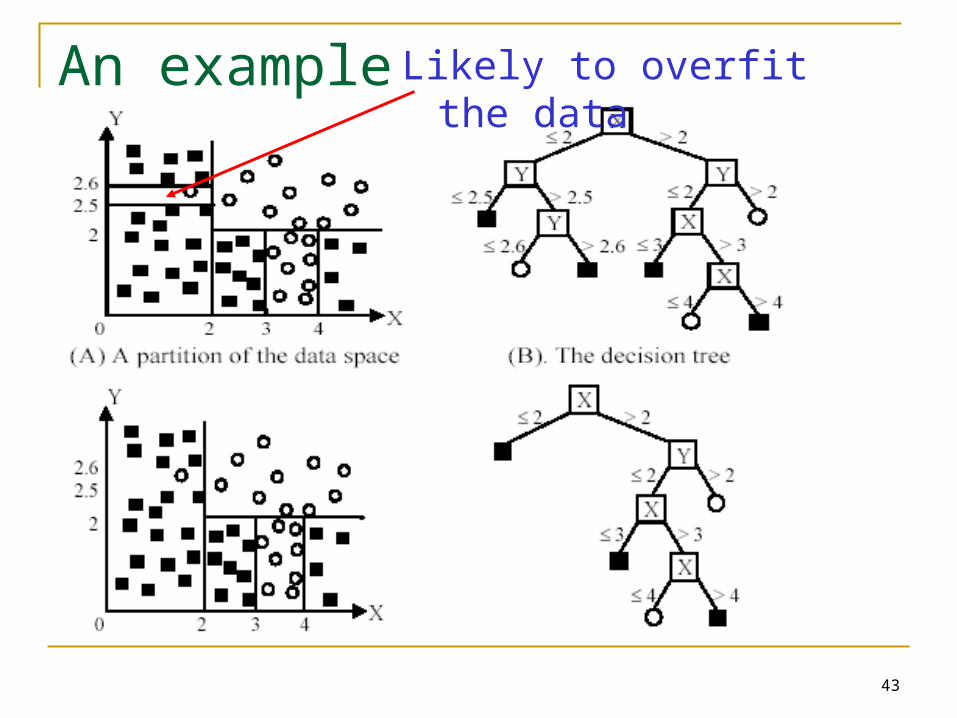
Avoid overfitting in classification Overfitting: A tree may overfit the training data

Good accuracy on training data but poor on test data Symptoms: tree too deep and too many branches,

some may reflect anomalies due to noise or outliers Two approaches to avoid overfitting

Pre-pruning: Halt tree construction early Difficult to decide because we do not know what may

happen subsequently if we keep growing the tree. Post-pruning: Remove branches or sub-trees from a

“fully grown” tree. This method is commonly used. C4.5 uses a statistical

method to estimates the errors at each node for pruning. A validation set may be used for pruning as well.

43

An example Likely to overfit the data

44

Other issues in decision tree learning From tree to rules, and rule pruning Handling of miss values Handing skewed distributions Handling attributes and classes with different

costs. Attribute construction Etc.

45


46

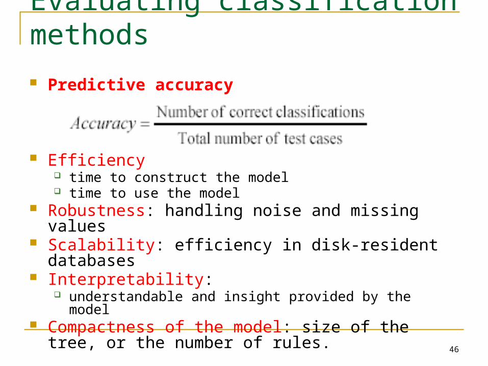
Evaluating classification methods

Predictive accuracy

Efficiency time to construct the model time to use the model

Robustness: handling noise and missing values Scalability: efficiency in disk-resident databases Interpretability:

understandable and insight provided by the model Compactness of the model: size of the tree, or the

number of rules.

47

Evaluation methods Holdout set: The available data set D is divided into

two disjoint subsets, the training set Dtrain (for learning a model) the test set Dtest (for testing the model)

Important: training set should not be used in testing and the test set should not be used in learning. Unseen test set provides a unbiased estimate of accuracy.

The test set is also called the holdout set. (the examples in the original data set D are all labeled with classes.)

This method is mainly used when the data set D is large.

48

Evaluation methods (cont…) n-fold cross-validation: The available data is

partitioned into n equal-size disjoint subsets. Use each subset as the test set and combine the rest

n-1 subsets as the training set to learn a classifier. The procedure is run n times, which give n

accuracies. The final estimated accuracy of learning is the

average of the n accuracies. 10-fold and 5-fold cross-validations are commonly

used. This method is used when the available data is not

large.

49

Evaluation methods (cont…)

Leave-one-out cross-validation: This method is used when the data set is very small.

It is a special case of cross-validation Each fold of the cross validation has only a

single test example and all the rest of the data is used in training.

If the original data has m examples, this is m-fold cross-validation

50

Evaluation methods (cont…) Validation set: the available data is divided into

three subsets, a training set, a validation set and a test set.

A validation set is used frequently for estimating parameters in learning algorithms.

In such cases, the values that give the best accuracy on the validation set are used as the final parameter values.

Cross-validation can be used for parameter estimating as well.

Training,Development, Test Sets Unseen test set

Avoid overfitting or tuning to the test set Don’t use test data for parameter tuning - use separate

validation/development data

Cross Validation over multiple splits Use Cross-validation for small data results over each split Compute pooled development set

performance

Training Set Development Set Test Set

Training Set Dev Set

Dev Set Training Set

Dev Set Trng SetTrng

Test Set

52

Classification measures Accuracy is only one measure (error = 1-accuracy). Accuracy is not suitable in some applications. In text mining, we may only be interested in the

documents of a particular topic, which are only a small portion of a big document collection.

In classification involving skewed or highly imbalanced data, e.g., NER, network intrusion and financial fraud detections, we are interested only in the minority class. High accuracy does not mean any intrusion is detected. E.g., 1% intrusion. Achieve 99% accuracy by doing nothing.

The class of interest is commonly called the positive class, and the rest negative classes.

53

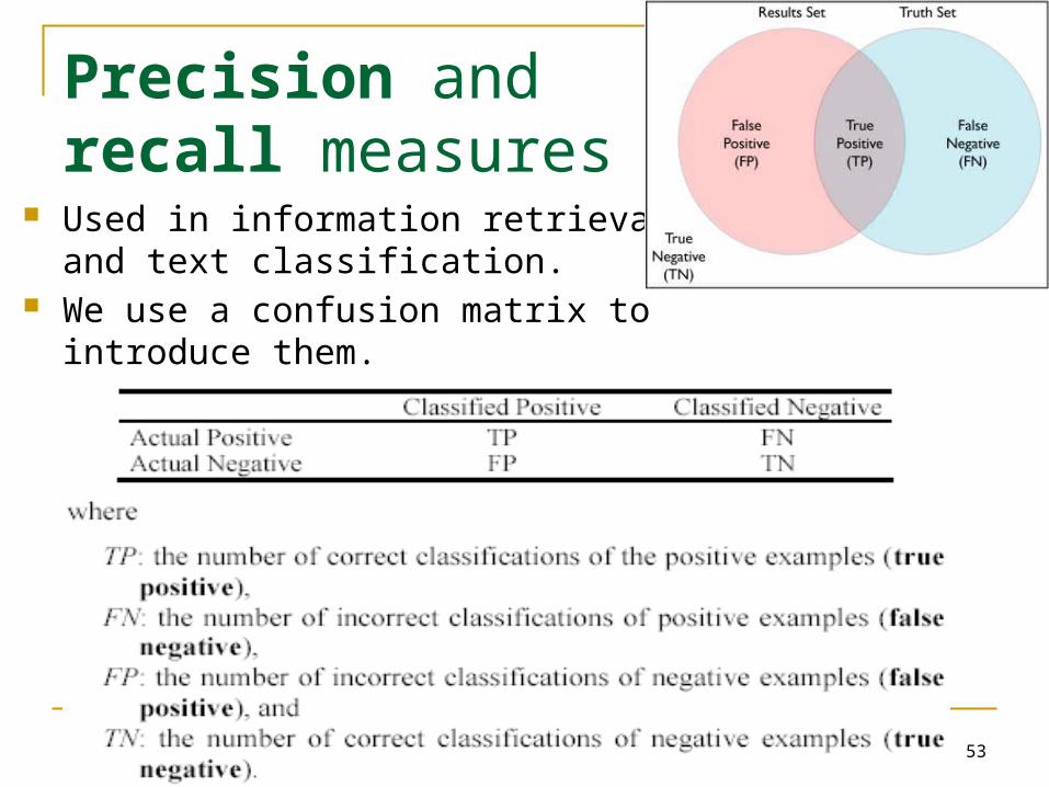
Precision and recall measures

Used in information retrieval and text classification.

We use a confusion matrix to introduce them.

Evaluation : Definitions

For a two-class classification problem: True Positive (TP) : The outcome is correctly

classified as positive. False Negative (FN) : The outcome is incorrectly

classified as negative when it is positive. False positive (FP): The outcome is incorrectly

classified as positive when it is negative. True Negative (TN): The outcome is correctly

classified as negative.

Evaluation : Definitions (2)

True Positive (TP) : Actual class of the test instance is positive and the classifier correctly predicts the class as positive

False Negative (FN) : Actual class of the test instance is positive but the classifier incorrectly predicts the class as negative

False positive (FP): Actual class of the test instance is negative but the classifier incorrectly predicts the class as positive

True Negative (TN) : Actual class of the test instance is negative and the classifier correctly predicts the class as negative

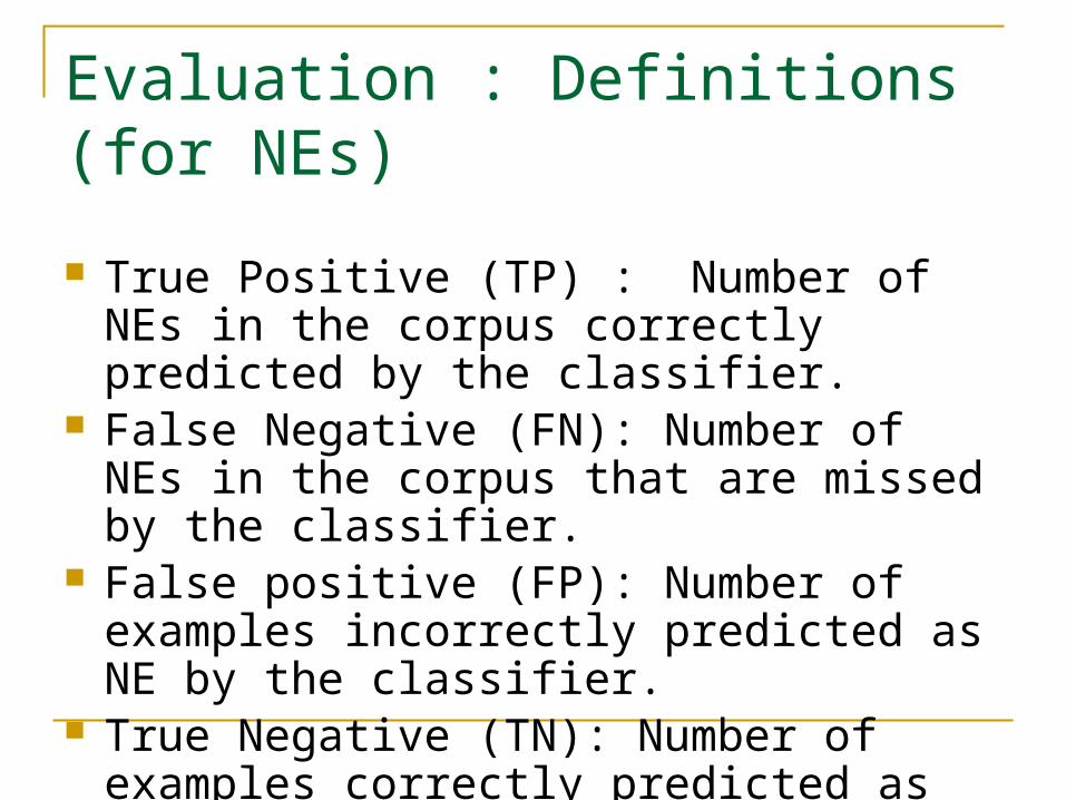
Evaluation : Definitions (for NEs)

True Positive (TP) : Number of NEs in the corpus correctly predicted by the classifier.

False Negative (FN): Number of NEs in the corpus that are missed by the classifier.

False positive (FP): Number of examples incorrectly predicted as NE by the classifier.

True Negative (TN): Number of examples correctly predicted as Outside

Evaluation for NEs

The classifier performance for classifying each multi token entity separately and the overall performance can be evaluated. At the left boundary At the right boundary At both boundaries

The metrics commonly used are Recall = sensitivity (% of correct items that are selected) Precision = specificity (% of selected items that are

correct) F-score = 2recallprecision/(recall+precision)

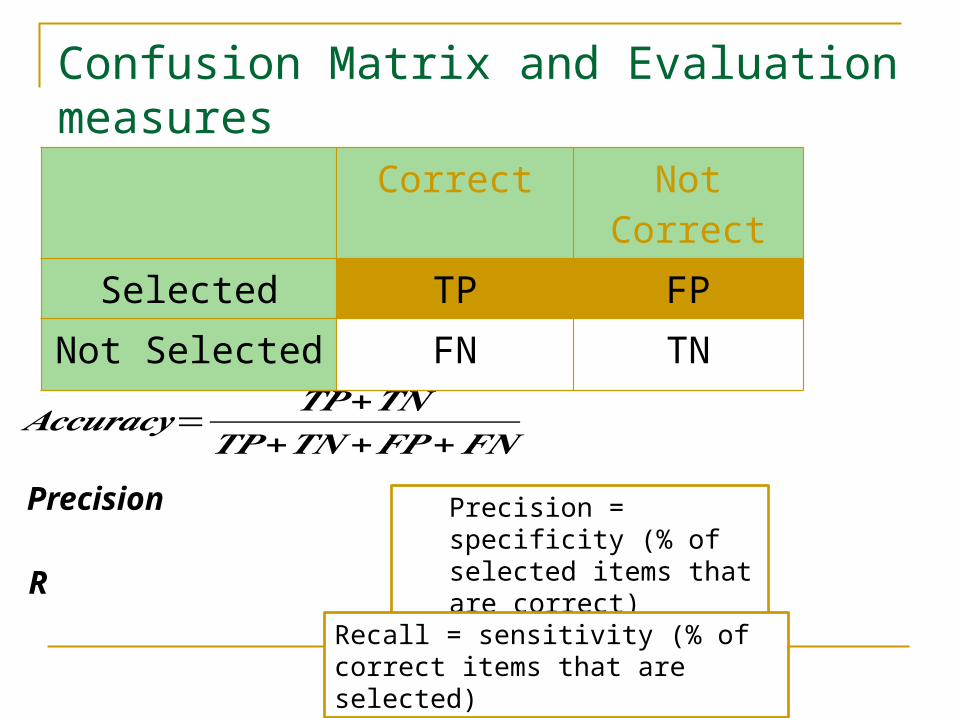
Confusion Matrix and Evaluation measures

Correct Not Correct

Selected TP FP

Not Selected FN TN

𝑨𝒄𝒄𝒖𝒓𝒂𝒄𝒚=𝑻𝑷+𝑻𝑵

𝑻𝑷+𝑻𝑵+𝑭𝑷+𝑭𝑵PrecisionR

Precision = specificity (% of selected items that are correct)

Recall = sensitivity (% of correct items that are selected)

59

An example

This confusion matrix gives precision p = 100% and recall r = 1%

because we only classified one positive example correctly and no negative examples wrongly.

Note: precision and recall only measure classification on the positive class.

. .FNTP

TP r

FPTP

TPp

60

F1-value (also called F1-score) It is hard to compare two classifiers using two measures. F1

score combines precision and recall into one measure

The harmonic mean of two numbers tends to be closer to the smaller of the two.

For F1-value to be large, both p and r much be large.

61

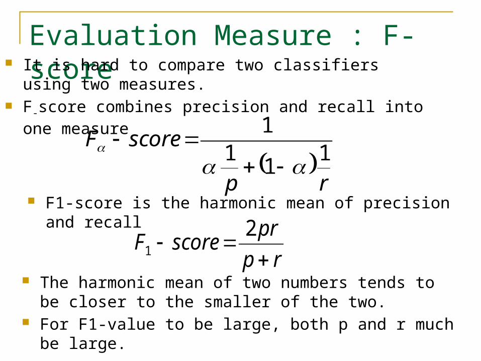
Evaluation Measure : F-score It is hard to compare two classifiers using two measures. F-score combines precision and recall into one measure

rp

scoreF1

11

1

F1-score is the harmonic mean of precision and recall

rp

prscoreF

21

The harmonic mean of two numbers tends to be closer to the smaller of the two.

For F1-value to be large, both p and r much be large.

Evaluation for each class: per-class measure Recall: Fraction of instances in class i that are

correctly classified

Precision: Fraction of instances assigned to class i that are actually in class i.

Accuracy: Fraction of documents classified correctly

Sample data

Confusion Matrix

Samples Predicted UK

Predicted poultry

Predicted wheat

Predicted coffee

Predicted interest

Predicted trade

Correct UK

95 1 13 0 1 0

Correct poultry

0 1 0 0 0 0

Correct wheat

10 90 0 1 0 0

Correct coffee

0 0 0 34 3 7

Correct interest

0 1 2 13 26 5

Correct trade

0 0 2 14 5 10

Evaluation for each class: per-class measure Recall: Fraction of instances in

class i that are correctly classified

Precision: Fraction of instances assigned to class i that are actually in class i.

Accuracy: Fraction of documents classified correctly

𝒄𝒊𝒊

∑𝒋𝒄 𝒊𝒋

𝒄 𝒊𝒊

∑𝒋𝒄 𝒋𝒊

∑𝒊

𝒄𝒊𝒊

∑𝒋∑𝒊

𝒄 𝒋𝒊

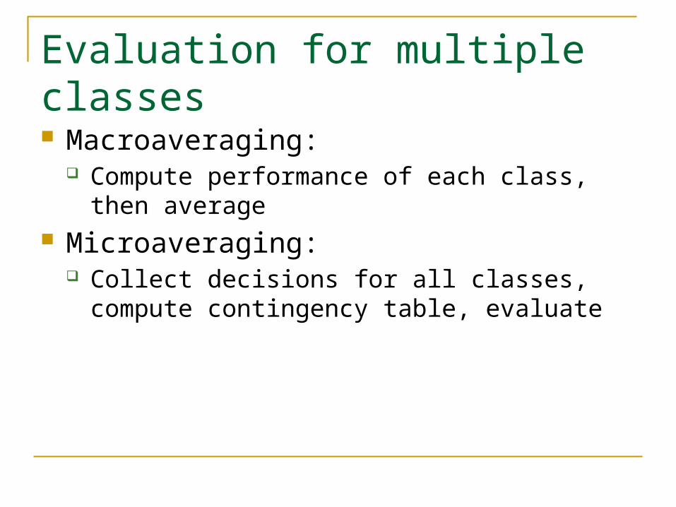
Evaluation for multiple classes Macroaveraging:

Compute performance of each class, then average

Microaveraging: Collect decisions for all classes, compute

contingency table, evaluate

Example: Micro vs Macro Averaging

CorrectYes

CorrectNo

Predicted Yes

10 10

Predicted No

10 970

CorrectYes

CorrectNo

Predicted Yes

90 10

Predicted No

10 890

CorrectYes

CorrectNo

Predicted Yes

100 20

Predicted No

20 1860

Class 1 Class 2 Micro Average

Macro Averaged Precision : ((10/(10+10) +(90/(90+10))/2=0.7

Micro Averaged Precision : 100/(20+100)=0.83

68


69

Introduction We showed that a decision tree can be

converted to a set of rules. if-then rules can be found directly from data

for classification Rule induction systems find a sequence of

rules (also called a decision list) for classification.

The commonly used strategy is sequential covering.

Sequential covering algorithms These algorithms generate the rules sequentially by looking for the

best rule that covers a subset of the examples Learn one rule at a time, sequentially.

We look for the rule with the best accuracy but not the maximum coverage

Once we have the best rule, we can eliminate the examples covered After a rule is learned, the training examples covered by the rule are

removed. Only the remaining data are used to find subsequent rules.

This procedure can be iterated until we have rules that cover all the dataset or some stopping criteria is met

The result is a disjunction of rules that can be ordered by accuracy

70

Note: a rule covers an example if the example satisfies the conditions of the rule.

Sequential covering algorithms - Algorithm

Algorithm: sequential-covering (attributes,examples,min)

list rules=[]

rule = learn-one-rule(attributes,examples)

while accuracy(rule,examples)>min and example is NOT NULL

loop

list rules= list rules + rule

examples = examples - correct-examples(rule, examples)

rule = learn-one-rule(attributes,examples)

end loop

list rules = order-by-accuracy(list rules)

71

Sequential covering algorithms

72

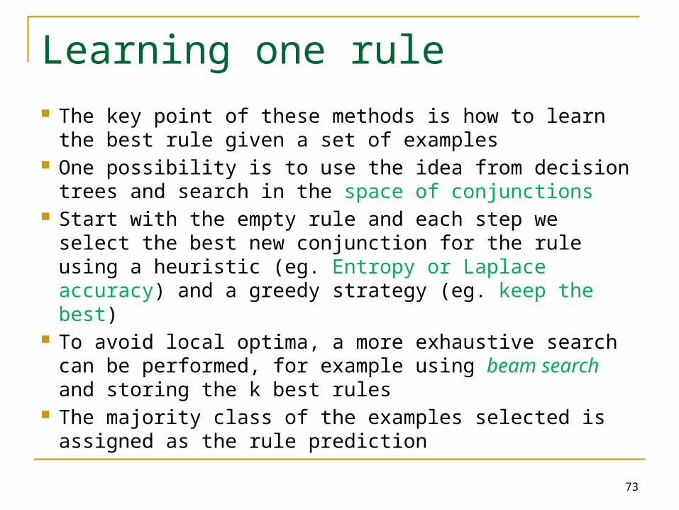
Learning one rule The key point of these methods is how to learn the best

rule given a set of examples One possibility is to use the idea from decision trees and

search in the space of conjunctions Start with the empty rule and each step we select the best

new conjunction for the rule using a heuristic (eg. Entropy or Laplace accuracy) and a greedy strategy (eg. keep the best)

To avoid local optima, a more exhaustive search can be performed, for example using beam search and storing the k best rules

The majority class of the examples selected is assigned as the rule prediction

73

Learn-One-Rule

The Learn-One-Rule procedure is normally implemented as general to specific beam search.

This is not the only way, but is reported to be the most efficient search technique.

It generates complexes from the most general, then greedily specialize those complexes until desired performance is reached.

Complex is conjunction of attribute-value specification. It forms the condition part in a rule, like "if condition then predict class".

74

Learn One Rule Algorithm1. Initialize a set of most general complexes.

2. Evaluate performances of those complexes over the example set.

i. Count how many positive and negative examples it covers.

ii. Evaluate their performances.

3. Sort complexes according to their performances.

4. If the best complex satisfies some threshold, form the hypothesis and return.

5. Otherwise, pick k best performing complexes for the next generation.

6. Specializing all k complexes in the set to find new set of less general complexes.

7. Go to step 2.

75

The number k is the beam factor of the search, meaning the maximum number of complexes to be specialized.

http://www.cse.unsw.edu.au/~cs9417ml/Rule/beamSearch.html#beam

http://www.cse.unsw.edu.au/~cs9417ml/Rule/beamSearch.html#beam

76

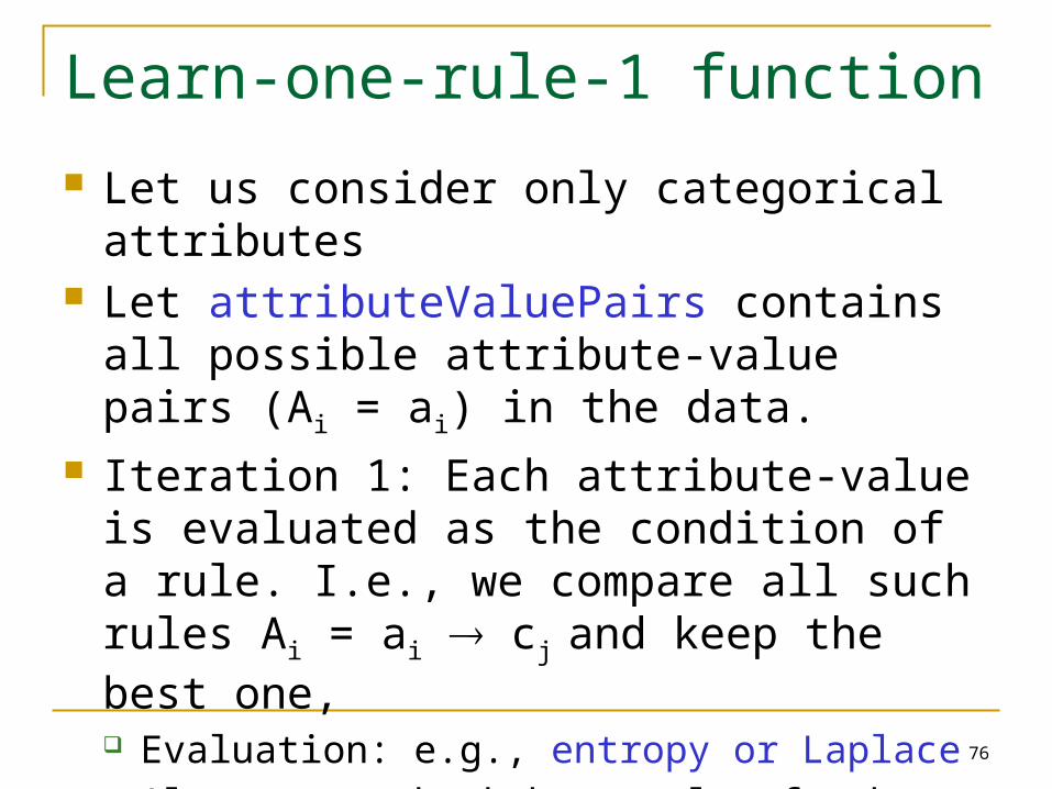
Learn-one-rule-1 function

Let us consider only categorical attributes Let attributeValuePairs contains all possible

attribute-value pairs (Ai = ai) in the data. Iteration 1: Each attribute-value is evaluated

as the condition of a rule. I.e., we compare all such rules Ai = ai cj and keep the best one, Evaluation: e.g., entropy or Laplace Also store the k best rules for beam search (to

search more space). Called new candidates.

77

Learn-one-rule-1 function (cont …) In iteration m, each (m-1)-condition rule in the new candidates set is expanded by attaching each attribute-value pair in attributeValuePairs as an additional condition to form candidate rules.

These new candidate rules are then evaluated in the same way as 1-condition rules. Update the best rule Update the k-best rules

The process repeats unless stopping criteria are met.

78

Discussions Accuracy: similar to decision tree Efficiency: Run much slower than decision tree

induction because To generate each rule, all possible rules are tried on the

data (not really all, but still a lot). When the data is large and/or the number of attribute-value

pairs are large. It may run very slowly. Rule interpretability: Can be a problem because

each rule is found after data covered by previous rules are removed. Thus, each rule may not be treated as independent of other rules.

79


80

Association rules for classification Classification: mine a small set of rules

existing in the data to form a classifier or predictor. It has a target attribute: Class attribute

Association rules: have no fixed target, but we can fix a target.

Class association rules (CAR): has a target class attribute. E.g.,

Own_house = true Class =Yes [sup=6/15, conf=6/6] CARs can obviously be used for classification.

81

Decision tree vs. CARs The decision tree below generates the following 3 rules.Own_house = true Class =Yes [sup=6/15, conf=6/6]Own_house = false, Has_job = true Class=Yes [sup=5/15, conf=5/5]Own_house = false, Has_job = false Class=No [sup=4/15, conf=4/4]

But there are many other rules that are not found by the decision tree

82

There are many more rules

CAR mining finds all of them.

In many cases, rules not in the decision tree (or a rule list) may perform classification better.

Such rules may also be actionable in practice

83

Decision tree vs. CARs (cont …) Association mining require discrete attributes.

Decision tree learning uses both discrete and continuous attributes. CAR mining requires continuous attributes

discretized. There are several such algorithms. Decision tree is not constrained by minsup or

minconf, and thus is able to find rules with very low support. Of course, such rules may be pruned due to the possible overfitting.

84

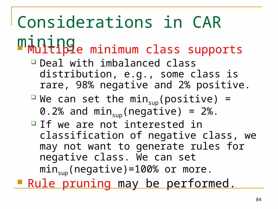
Considerations in CAR mining Multiple minimum class supports

Deal with imbalanced class distribution, e.g., some class is rare, 98% negative and 2% positive.

We can set the minsup(positive) = 0.2% and minsup(negative) = 2%.

If we are not interested in classification of negative class, we may not want to generate rules for negative class. We can set minsup(negative)=100% or more.

Rule pruning may be performed.

85

Building classifiers There are many ways to build classifiers using

CARs. Several existing systems available. Simplest: After CARs are mined, do nothing.

For each test case, we simply choose the most confident rule that covers the test case to classify it. Microsoft SQL Server has a similar method.

Or, using a combination of rules. Another method (used in the CBA system) is

similar to sequential covering. Choose a set of rules to cover the training data.

86

Rules are sorted first

Definition: Given two rules, ri and rj, ri rj (also called ri precedes rj or ri has a higher precedence than rj) if the confidence of ri is greater than that of rj, or their confidences are the same, but the support of

ri is greater than that of rj, or both the confidences and supports of ri and rj are

the same, but ri is generated earlier than rj.

A CBA classifier L is of the form:

L = <r1, r2, …, rk, default-class>

87

Classifier building using CARs

This algorithm is very inefficient CBA has very efficient algorithm that scans the

data at most two times (quite involved).

88


89

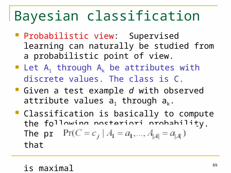
Bayesian classification Probabilistic view: Supervised learning can naturally

be studied from a probabilistic point of view. Let A1 through Ak be attributes with discrete values.

The class is C. Given a test example d with observed attribute

values a1 through ak.

Classification is basically to compute the following posteriori probability. The prediction is the class cj such that

is maximal

90

Apply Bayes’ Rule

Pr(C=cj) is the class prior probability: easy to estimate from the training data.

||

1||||11

||||11

||||11

||||11

||||11

)Pr()|,...,Pr(

)Pr()|,...,Pr(

),...,Pr(

)Pr()|,...,Pr(

),...,|Pr(

C

rrrAA

jjAA

AA

jjAA

AAj

cCcCaAaA

cCcCaAaA

aAaA

cCcCaAaA

aAaAcC

91

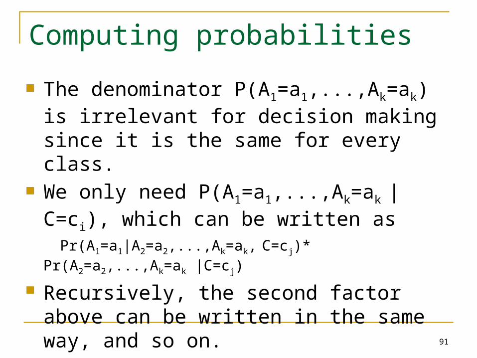
Computing probabilities

The denominator P(A1=a1,...,Ak=ak) is irrelevant for decision making since it is the same for every class.

We only need P(A1=a1,...,Ak=ak | C=ci), which can be written as

Pr(A1=a1|A2=a2,...,Ak=ak, C=cj)* Pr(A2=a2,...,Ak=ak |C=cj)

Recursively, the second factor above can be written in the same way, and so on.

Now an assumption is needed.

92

Conditional independence assumption All attributes are conditionally independent

given the class C = cj. Formally, we assume, Pr(A1=a1 | A2=a2, ..., A|A|=a|A|, C=cj) = Pr(A1=a1 | C=cj)

and so on for A2 through A|A|. I.e.,

||

1||||11 )|Pr()|,...,Pr(

A

ijiiiAA cCaAcCaAaA

93

Final naïve Bayesian classifier

We are done! How do we estimate P(Ai = ai| C=cj)? Easy!.

||

1

||

1

||

1

||||11

)|Pr()Pr(

)|Pr()Pr(

),...,|Pr(

C

r

A

iriir

A

ijiij

AAj

cCaAcC

cCaAcC

aAaAcC

94

Classify a test instance If we only need a decision on the most

probable class for the test instance, we only need the numerator as its denominator is the same for every class.

Thus, given a test example, we compute the following to decide the most probable class for the test instance

||

1

)|Pr()Pr(maxarg A

ijiij

ccCaAcc

j

95

An example

Compute all probabilities required for classification

96

An Example (cont …)

For C = t, we have

For class C = f, we have

C = t is more probable. t is the final class.

25

2

5

2

5

2

2

1)|Pr()Pr(

2

1

j

jj tCaAtC

25

1

5

2

5

1

2

1)|Pr()Pr(

2

1

j

jj fCaAfC

97

Additional issues Numeric attributes: Naïve Bayesian

learning assumes that all attributes are categorical. Numeric attributes need to be discretized.

Zero counts: An particular attribute value never occurs together with a class in the training set. We need smoothing.

Missing values: Ignored

ij

ijjii nn

ncCaA

)|Pr(

98

On naïve Bayesian classifier

Advantages: Easy to implement Very efficient Good results obtained in many applications

Disadvantages Assumption: class conditional independence,

therefore loss of accuracy when the assumption is seriously violated (those highly correlated data sets)

99


100

Text classification/categorization Due to the rapid growth of online documents in

organizations and on the Web, automated document classification has become an important problem.

Techniques discussed previously can be applied to text classification, but they are not as effective as the next three methods.

We first study a naïve Bayesian method specifically formulated for texts, which makes use of some text specific features.

However, the ideas are similar to the preceding method.

101

Probabilistic framework Generative model: Each document is

generated by a parametric distribution governed by a set of hidden parameters.

The generative model makes two assumptions

The data (or the text documents) are generated by a mixture model,

There is one-to-one correspondence between mixture components and document classes.

102

Mixture model A mixture model models the data with a

number of statistical distributions. Intuitively, each distribution corresponds to a data

cluster and the parameters of the distribution provide a description of the corresponding cluster.

Each distribution in a mixture model is also called a mixture component.

The distribution/component can be of any kind

103

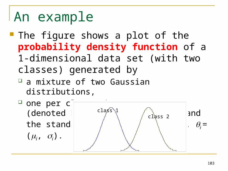
An example The figure shows a plot of the probability

density function of a 1-dimensional data set (with two classes) generated by a mixture of two Gaussian distributions, one per class, whose parameters (denoted by i) are

the mean (i) and the standard deviation (i), i.e., i = (i, i).

class 1 class 2

104

Mixture model (cont …)

Let the number of mixture components (or distributions) in a mixture model be K.

Let the jth distribution have the parameters j. Let be the set of parameters of all

components, = {1, 2, …, K, 1, 2, …, K}, where j is the mixture weight (or mixture probability) of the mixture component j and j is the parameters of component j.

How does the model generate documents?

105

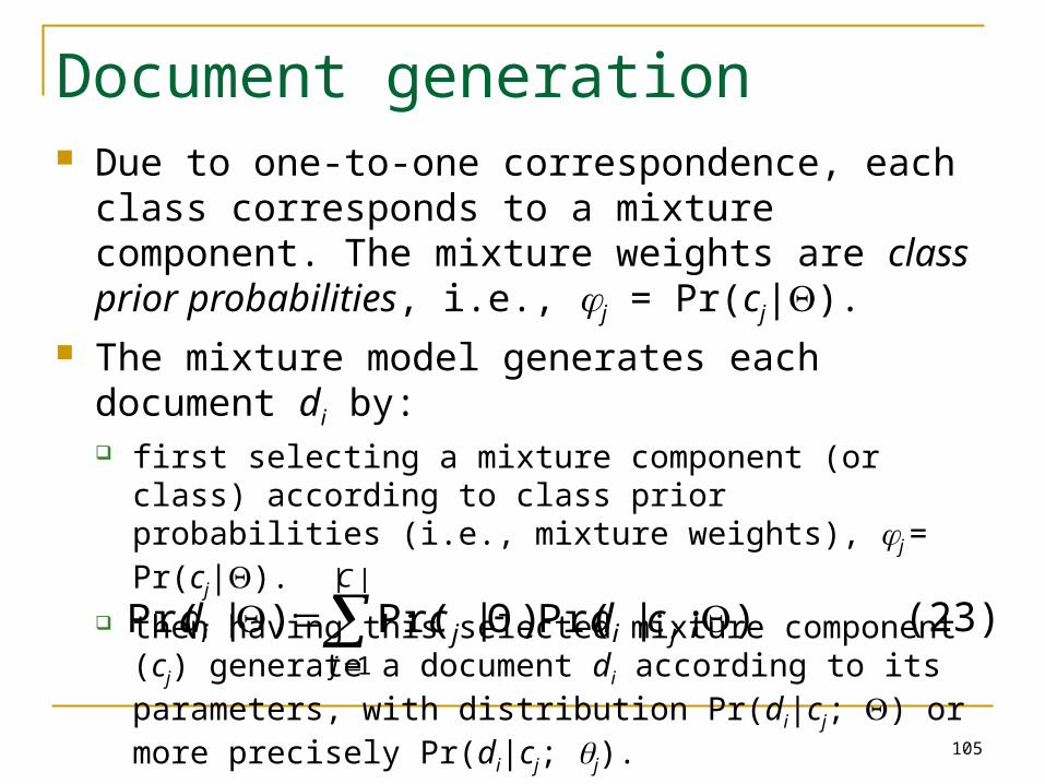
Document generation Due to one-to-one correspondence, each class

corresponds to a mixture component. The mixture weights are class prior probabilities, i.e., j = Pr(cj|).

The mixture model generates each document di by: first selecting a mixture component (or class) according to

class prior probabilities (i.e., mixture weights), j = Pr(cj|). then having this selected mixture component (cj) generate

a document di according to its parameters, with distribution Pr(di|cj; ) or more precisely Pr(di|cj; j).

) ;|Pr()Θ|Pr()|Pr(||

1

C

jjiji cdcd (23)

106

Model text documents The naïve Bayesian classification treats each

document as a “bag of words”. The generative model makes the following further assumptions: Words of a document are generated

independently of context given the class label. The familiar naïve Bayes assumption used before.

The probability of a word is independent of its position in the document. The document length is chosen independent of its class.

107

Multinomial distribution

With the assumptions, each document can be regarded as generated by a multinomial distribution.

In order words, each document is drawn from a multinomial distribution of words with as many independent trials as the length of the document.

The words are from a given vocabulary V = {w1, w2, …, w|V|}.

108

Use probability function of multinomial distribution

where Nti is the number of times that word wt occurs in document di and

||

1 !

);|Pr(|!||)Pr(|);|Pr(

V

t ti

tiNjt

iiji

N

cwddcd

||||

1

i

V

t

it dN

.1);|Pr(||

1

V

t

jt cw

(24)

(25)

109

Parameter estimation The parameters are estimated based on empirical

counts.

In order to handle 0 counts for infrequent occurring words that do not appear in the training set, but may appear in the test set, we need to smooth the probability. Lidstone smoothing, 0 1

.)|Pr(

)|Pr()ˆ;|Pr(

||

1

||

1

||

1

V

s

D

i ijsi

D

i ijti

jtdcN

dcNcw

.)|Pr(||

)|Pr()ˆ;|Pr(

||

1

||

1

||

1

V

s

D

i ijsi

D

i ijti

jtdcNV

dcNcw

(26)

(27)

110

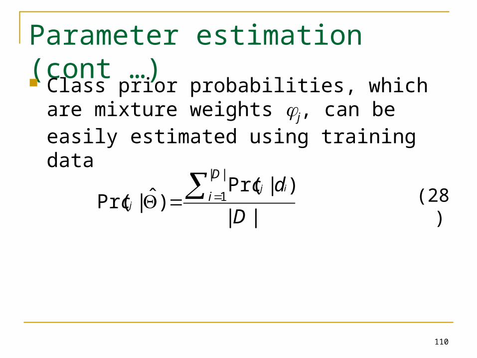
Parameter estimation (cont …) Class prior probabilities, which are mixture

weights j, can be easily estimated using training data

||

)|Pr()ˆ|Pr(

||

1

D

dcc

D

iij

j (28)

111

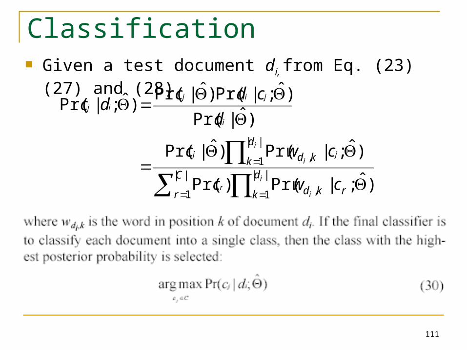
Classification Given a test document di, from Eq. (23) (27) and (28)

||

1

||

1 ,

||

1 ,

)ˆ;|Pr()Pr(

)ˆ;|Pr()ˆ|Pr(

)ˆ|Pr(

)ˆ;|Pr()ˆ|Pr()ˆ;|Pr(

C

r

d

k rkd

d

k kd

i

ir

ij

ij

i

jij

ij

cwc

cwc

d

cdcdc

112

Discussions Most assumptions made by naïve Bayesian

learning are violated to some degree in practice.

Despite such violations, researchers have shown that naïve Bayesian learning produces very accurate models. The main problem is the mixture model

assumption. When this assumption is seriously violated, the classification performance can be poor.

Naïve Bayesian learning is extremely efficient.

113


114

Introduction Support vector machines were invented by V.

Vapnik and his co-workers in 1970s in Russia and became known to the West in 1992.

SVMs are linear classifiers that find a hyperplane to separate two class of data, positive and negative.

Kernel functions are used for nonlinear separation. SVM not only has a rigorous theoretical foundation,

but also performs classification more accurately than most other methods in applications, especially for high dimensional data.

It is perhaps the best classifier for text classification.

115

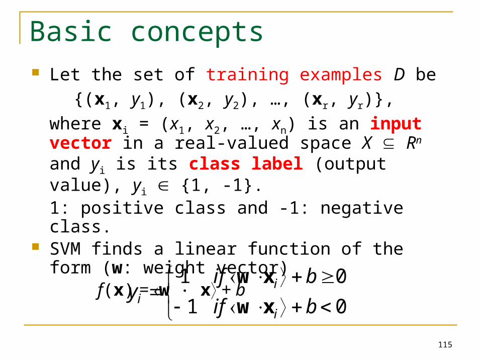
Basic concepts Let the set of training examples D be

{(x1, y1), (x2, y2), …, (xr, yr)},

where xi = (x1, x2, …, xn) is an input vector in a real-valued space X Rn and yi is its class label (output value), yi {1, -1}. 1: positive class and -1: negative class.

SVM finds a linear function of the form (w: weight vector)

f(x) = w x + b

01

01

bif

bify

i

ii xw

xw

116

The hyperplane The hyperplane that separates positive and negative

training data is

w x + b = 0 It is also called the decision boundary (surface). So many possible hyperplanes, which one to

choose?

117

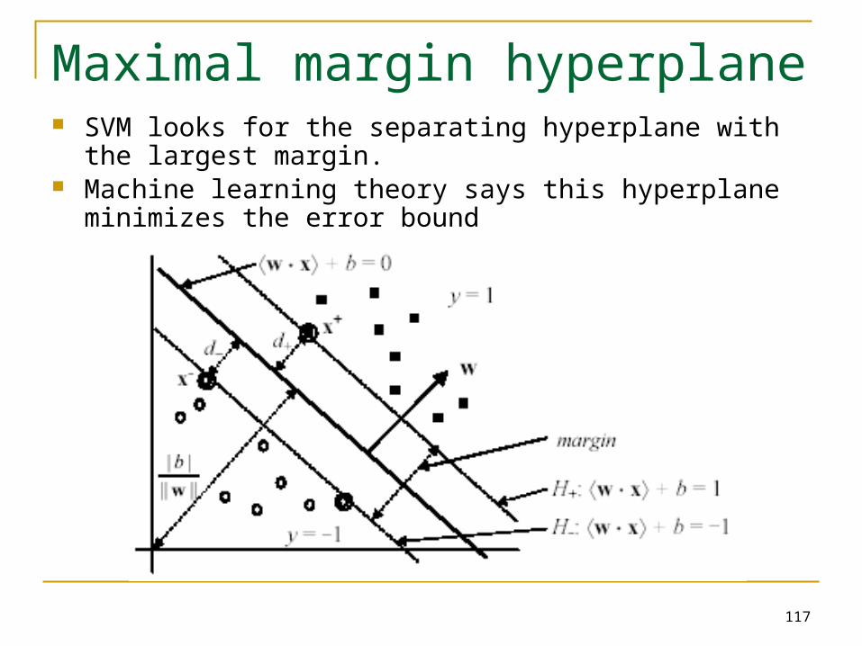
Maximal margin hyperplane SVM looks for the separating hyperplane with the largest

margin. Machine learning theory says this hyperplane minimizes the

error bound

118

Linear SVM: separable case Assume the data are linearly separable. Consider a positive data point (x+, 1) and a negative

(x-, -1) that are closest to the hyperplane <w x> + b = 0.

We define two parallel hyperplanes, H+ and H-, that pass through x+ and x- respectively. H+ and H- are also parallel to <w x> + b = 0.

119

Compute the margin Now let us compute the distance between the two

margin hyperplanes H+ and H-. Their distance is the margin (d+ + d in the figure).

Recall from vector space in algebra that the (perpendicular) distance from a point xi to the hyperplane w x + b = 0 is:

where ||w|| is the norm of w,

||||

||

w

xw bi

222

21 ...|||| nwww www

(36)

(37)

120

Compute the margin (cont …) Let us compute d+. Instead of computing the distance from x+ to the

separating hyperplane w x + b = 0, we pick up any point xs on w x + b = 0 and compute the distance from xs to w x+ + b = 1 by applying the distance Eq. (36) and noticing w xs + b = 0,

||||

1

||||

|1|

ww

xw s

b

d

||||

2

w ddmargin

(38)

(39)

121

A optimization problem!Definition (Linear SVM: separable case): Given a set of

linearly separable training examples,

D = {(x1, y1), (x2, y2), …, (xr, yr)}

Learning is to solve the following constrained minimization problem,

summarizes

w xi + b 1 for yi = 1w xi + b -1 for yi = -1.

riby ii ..., 2, 1, ,1)( :Subject to2

:Minimize

xw

ww

riby ii ..., 2, 1, ,1( xw

(40)

122

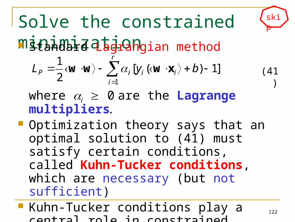
Solve the constrained minimization Standard Lagrangian method

where i 0 are the Lagrange multipliers. Optimization theory says that an optimal

solution to (41) must satisfy certain conditions, called Kuhn-Tucker conditions, which are necessary (but not sufficient)

Kuhn-Tucker conditions play a central role in constrained optimization.

]1)([2

1

1

byL i

r

iiiP xwww (41)

skip

123

Kuhn-Tucker conditions

Eq. (50) is the original set of constraints. The complementarity condition (52) shows that only those

data points on the margin hyperplanes (i.e., H+ and H-) can have i > 0 since for them yi(w xi + b) – 1 = 0.

These points are called the support vectors, All the other parameters i = 0.

skip

124

Solve the problem In general, Kuhn-Tucker conditions are necessary

for an optimal solution, but not sufficient. However, for our minimization problem with a

convex objective function and linear constraints, the Kuhn-Tucker conditions are both necessary and sufficient for an optimal solution.

Solving the optimization problem is still a difficult task due to the inequality constraints.

However, the Lagrangian treatment of the convex optimization problem leads to an alternative dual formulation of the problem, which is easier to solve than the original problem (called the primal).

125

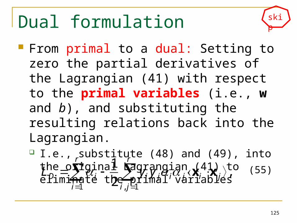
Dual formulation From primal to a dual: Setting to zero the

partial derivatives of the Lagrangian (41) with respect to the primal variables (i.e., w and b), and substituting the resulting relations back into the Lagrangian. I.e., substitute (48) and (49), into the original

Lagrangian (41) to eliminate the primal variables

(55),2

1

1,1

ji

r

jijiji

r

iiD yyL xx

skip

126

Dual optimization prolem

This dual formulation is called the Wolfe dual. For the convex objective function and linear constraints of

the primal, it has the property that the maximum of LD occurs at the same values of w, b and i, as the minimum of LP (the primal).

Solving (56) requires numerical techniques and clever

strategies, which are beyond our scope.

skip

127

The final decision boundary After solving (56), we obtain the values for i, which

are used to compute the weight vector w and the bias b using Equations (48) and (52) respectively.

The decision boundary

Testing: Use (57). Given a test instance z,

If (58) returns 1, then the test instance z is classified as positive; otherwise, it is classified as negative.

0

bybsvi

iii xxxw (57)

sviiii bysignbsign zxzw )( (58)

128

Linear SVM: Non-separable case Linear separable case is the ideal situation. Real-life data may have noise or errors.

Class label incorrect or randomness in the application domain.

Recall in the separable case, the problem was

With noisy data, the constraints may not be satisfied. Then, no solution!

riby ii ..., 2, 1, ,1)( :Subject to2

:Minimize

xw

ww

129

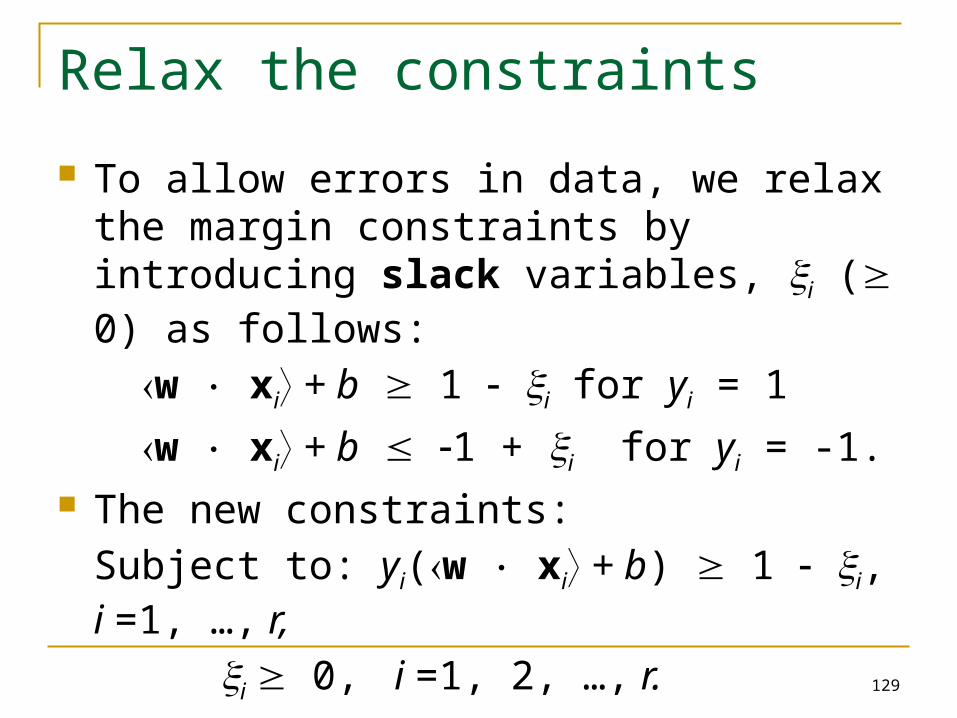
Relax the constraints

To allow errors in data, we relax the margin constraints by introducing slack variables, i ( 0) as follows:

w xi + b 1 i for yi = 1

w xi + b 1 + i for yi = -1. The new constraints:

Subject to: yi(w xi + b) 1 i, i =1, …, r,

i 0, i =1, 2, …, r.

130

Geometric interpretation Two error data points xa and xb (circled) in wrong

regions

131

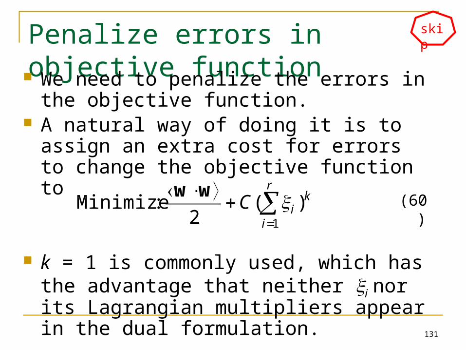
Penalize errors in objective function We need to penalize the errors in the

objective function. A natural way of doing it is to assign an extra

cost for errors to change the objective function to

k = 1 is commonly used, which has the advantage that neither i nor its Lagrangian multipliers appear in the dual formulation.

r

i

kiC

1

)(2

:Minimize ww (60)

skip

132

New optimization problem

This formulation is called the soft-margin SVM. The primal Lagrangian is

where i, i 0 are the Lagrange multipliers

ri

riby

C

i

iii

r

ii

..., 2, 1, ,0

..., 2, 1, ,1)( :Subject to

2 :Minimize

1

xw

ww(61)

r

iiiii

r

iii

r

iiP byCL

111

]1)([2

1 xwww

(62)

skip

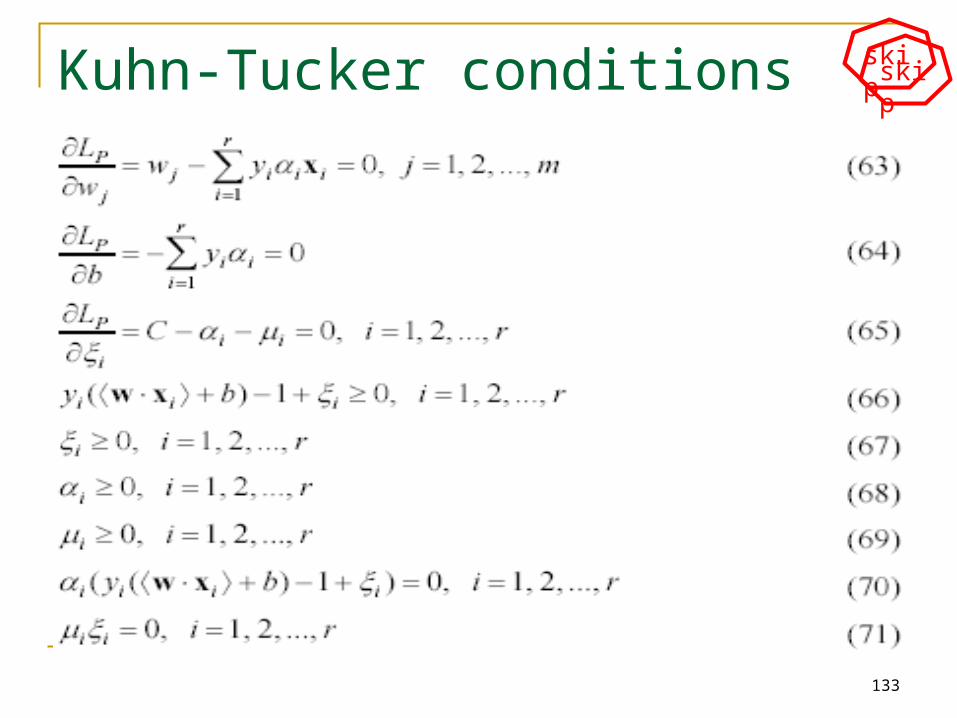
133

Kuhn-Tucker conditions skipskip

134

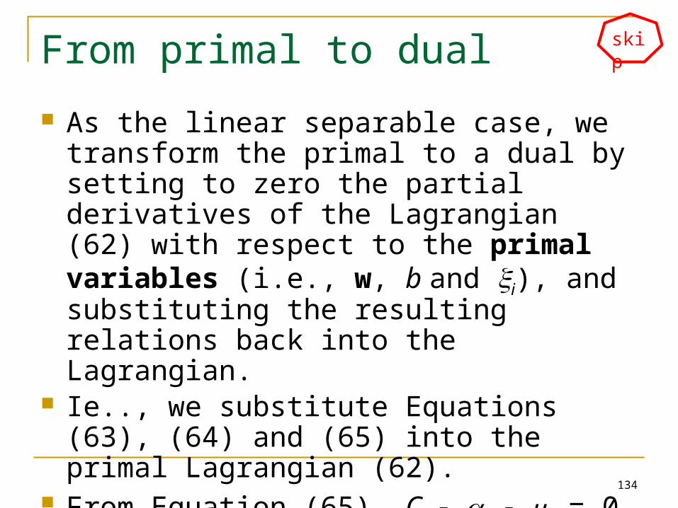
From primal to dual

As the linear separable case, we transform the primal to a dual by setting to zero the partial derivatives of the Lagrangian (62) with respect to the primal variables (i.e., w, b and i), and substituting the resulting relations back into the Lagrangian.

Ie.., we substitute Equations (63), (64) and (65) into the primal Lagrangian (62).

From Equation (65), C i i = 0, we can deduce that i C because i 0.

skip

135

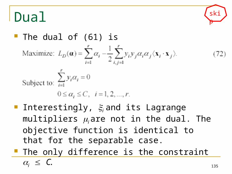
Dual The dual of (61) is

Interestingly, i and its Lagrange multipliers i are not in the dual. The objective function is identical to that for the separable case.

The only difference is the constraint i C.

skip

136

Find primal variable values The dual problem (72) can be solved numerically. The resulting i values are then used to compute w

and b. w is computed using Equation (63) and b is computed using the Kuhn-Tucker complementarity conditions (70) and (71).

Since no values for i, we need to get around it. From Equations (65), (70) and (71), we observe that if 0 < i

< C then both i = 0 and yiw xi + b – 1 + i = 0. Thus, we can use any training data point for which 0 < i < C and Equation (69) (with i = 0) to compute b.

.01

1

j

r

iiii

i

yy

b xx (73)

skip

137

(65), (70) and (71) in fact tell us more

(74) shows a very important property of SVM. The solution is sparse in i. Many training data points are

outside the margin area and their i’s in the solution are 0. Only those data points that are on the margin (i.e., yi(w xi

+ b) = 1, which are support vectors in the separable case), inside the margin (i.e., i = C and yi(w xi + b) < 1), or errors are non-zero.

Without this sparsity property, SVM would not be practical for large data sets.

skip

138

The final decision boundary

The final decision boundary is (we note that many i’s are 0)

The decision rule for classification (testing) is the same as the separable case, i.e.,

sign(w x + b).

Finally, we also need determine the parameter C in the objective function. It is normally chosen through the use of a validation set or cross-validation.

01

bybr

iiii xxxw (75)

139

How to deal with nonlinear separation? The SVM formulations require linear separation. Real-life data sets may need nonlinear separation. To deal with nonlinear separation, the same

formulation and techniques as for the linear case are still used.

We only transform the input data into another space (usually of a much higher dimension) so that a linear decision boundary can separate positive and

negative examples in the transformed space, The transformed space is called the feature space.

The original data space is called the input space.

140

Space transformation

The basic idea is to map the data in the input space X to a feature space F via a nonlinear mapping ,

After the mapping, the original training data set {(x1, y1), (x2, y2), …, (xr, yr)} becomes:

{((x1), y1), ((x2), y2), …, ((xr), yr)}

)(

:

xx

FX (76)

(77)

141

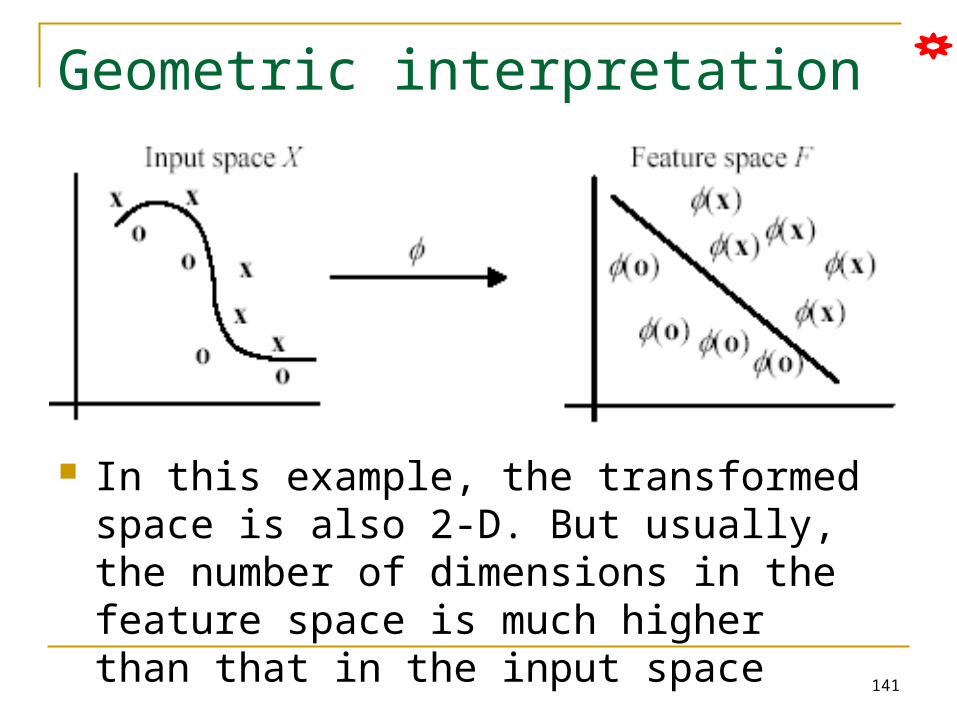
Geometric interpretation

In this example, the transformed space is also 2-D. But usually, the number of dimensions in the feature space is much higher than that in the input space

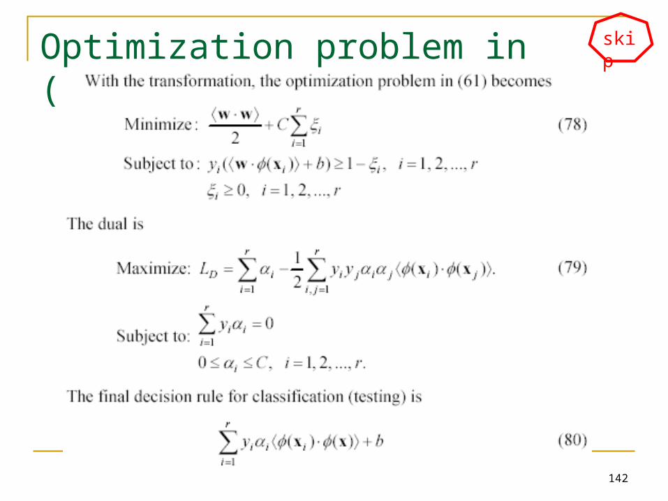
142

Optimization problem in (61) becomes

skip

143

An example space transformation Suppose our input space is 2-dimensional,

and we choose the following transformation (mapping) from 2-D to 3-D:

The training example ((2, 3), -1) in the input space is transformed to the following in the feature space:

((4, 9, 8.5), -1)

)2 , ,() ,( 212

22

121 xxxxxx

144

Problem with explicit transformation The potential problem with this explicit data

transformation and then applying the linear SVM is that it may suffer from the curse of dimensionality.

The number of dimensions in the feature space can be huge with some useful transformations even with reasonable numbers of attributes in the input space.

This makes it computationally infeasible to handle. Fortunately, explicit transformation is not needed.

145

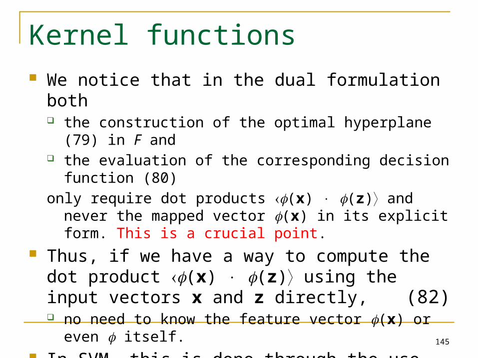
Kernel functions We notice that in the dual formulation both

the construction of the optimal hyperplane (79) in F and the evaluation of the corresponding decision function (80)

only require dot products (x) (z) and never the mapped vector (x) in its explicit form. This is a crucial point.

Thus, if we have a way to compute the dot product (x) (z) using the input vectors x and z directly, no need to know the feature vector (x) or even itself.

In SVM, this is done through the use of kernel functions, denoted by K,

K(x, z) = (x) (z) (82)

146

An example kernel function Polynomial kernel

K(x, z) = x zd Let us compute the kernel with degree d = 2 in a 2-

dimensional space: x = (x1, x2) and z = (z1, z2).

This shows that the kernel x z2 is a dot product in a transformed feature space

(83)

,)()(

)2()2(

2

)(

2222

2222

22

122

1122

1

2211

21

21

211

2

zx

zx

zz,z,zxx,x,x

zxzxzxzx

zxzx(84)

147

Kernel trick The derivation in (84) is only for illustration

purposes. We do not need to find the mapping function. We can simply apply the kernel function

directly by replace all the dot products (x) (z) in (79) and

(80) with the kernel function K(x, z) (e.g., the polynomial kernel x zd in (83)).

This strategy is called the kernel trick.

148

Is it a kernel function?

The question is: how do we know whether a function is a kernel without performing the derivation such as that in (84)? I.e, How do we know that a kernel function is indeed a

dot product in some feature space? This question is answered by a theorem

called the Mercer’s theorem, which we will not discuss here.

149

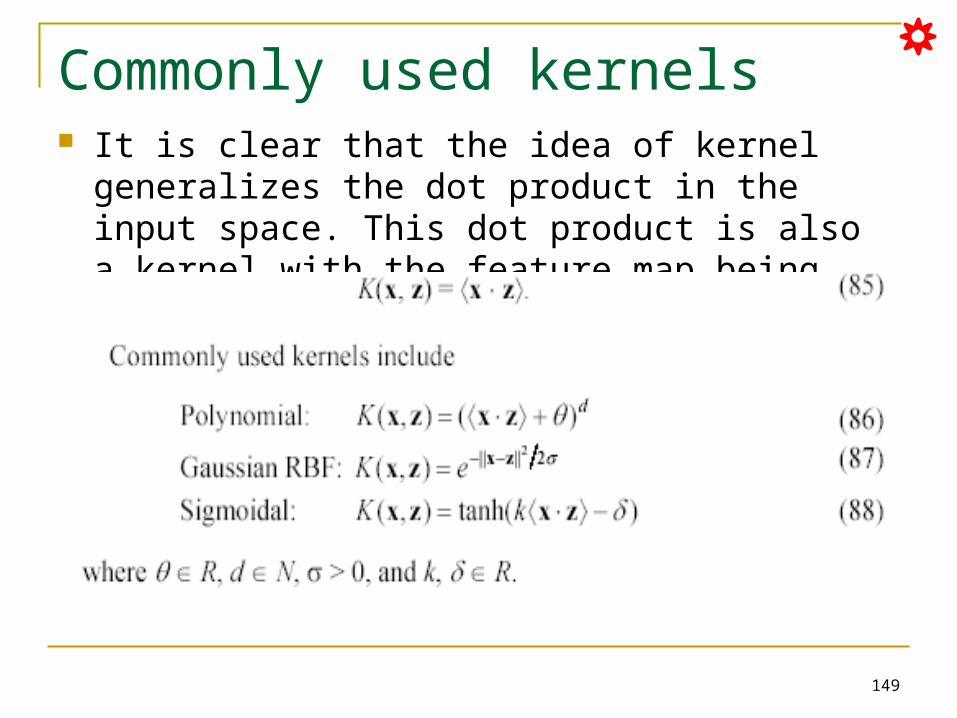
Commonly used kernels It is clear that the idea of kernel generalizes the dot

product in the input space. This dot product is also a kernel with the feature map being the identity

150

Some other issues in SVM SVM works only in a real-valued space. For a

categorical attribute, we need to convert its categorical values to numeric values.

SVM does only two-class classification. For multi-class problems, some strategies can be applied, e.g., one-against-rest, and error-correcting output coding.

The hyperplane produced by SVM is hard to understand by human users. The matter is made worse by kernels. Thus, SVM is commonly used in applications that do not require human understanding.

151


152

k-Nearest Neighbor Classification (kNN) Unlike all the previous learning methods, kNN

does not build model from the training data. To classify a test instance d, define k-

neighborhood P as k nearest neighbors of d Count number n of training instances in P that

belong to class cj

Estimate Pr(cj|d) as n/k No training is needed. Classification time is

linear in training set size for each test case.

153

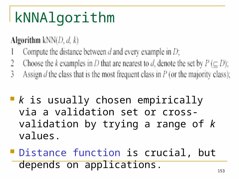
kNNAlgorithm

k is usually chosen empirically via a validation set or cross-validation by trying a range of k values.

Distance function is crucial, but depends on applications.

154

Example: k=6 (6NN)

Government

Science

Arts

A new point Pr(science| )?

155

Discussions kNN can deal with complex and arbitrary

decision boundaries. Despite its simplicity, researchers have

shown that the classification accuracy of kNN can be quite strong and in many cases as accurate as those elaborated methods.

kNN is slow at the classification time kNN does not produce an understandable

model

156


157

Summary Applications of supervised learning are in almost

any field or domain. We studied 8 classification techniques. There are still many other methods, e.g.,

Bayesian networks Neural networks Genetic algorithms Fuzzy classification

This large number of methods also show the importance of classification and its wide applicability.

It remains to be an active research area.

supervised learning. introduction 3 why “learn”? machine learning is programming computers to...

Documents