Sustaining Groundwater: Role of Policy Reforms in Promoting Conservation in India*

Sheetal Sekhri†

This Draft: January , 2013

Abstract

Groundwater depletion has become an increasingly important policy concern in many

countries around the world especially so in India, which is the largest user of groundwater for

irrigation. Groundwater is contended to have ushered green revolution in the country. However,

a downside to this pattern of development is that it is not sustainable. As in other countries, the

stocks of groundwater are rapidly depleting in India. Against this backdrop, it is important to

understand what policies can help conserve this vital resource. This study uses data from

observation and monitoring wells of the country to identify depletion hot-spots and evaluate the

impact of two policies- rainwater harvesting mandates and delaying of paddy transplanting time-

on water tables. Rain water harvesting mandates did not have beneficial effects on water tables in

the short run and delayed transplanting of paddy resulted in increased use of groundwater.

Keywords: Groundwater, India

* I wish to thank the Central Ground Water Board (CGWB) of India for providing the groundwater data. Daniel Muldoon provided excellent research assistance. † University of Virginia, Email: SSekhri@virginia.edu

1

1 Introduction

India is the largest user of groundwater for irrigation in the world. The amount of groundwater

drawn is estimated to be 230 billion cubic meters per year (in 2004) compared to 101 billion

cubic meters in China and 108 billion cubic meters in US in 2005 (FAO, Aquastat dataset).

Indian agriculture is sustained by groundwater. According to the 2005-06 Agricultural Census of

the country, 60.4 percent of the net irrigated area is irrigated using groundwater. Agriculture is

the source of livelihood for majority of Indian population. In 2009-10, agriculture employed 52.9

percent of the working population (National Sample Survey Organization, 2011). In addition,

around 80 percent of the rural population relies on groundwater for meeting their drinking water

needs.

Groundwater is contended to have ushered green revolution in the country (Repetto,

1994; Shah et al 2007). Groundwater irrigation has ensured food security in times of deficit

rainfall and facilitated a manifold increase in agricultural productivity. The country has become a

net exporter of food grains. However, this pattern of development is not sustainable. As in other

countries, the stocks of groundwater are rapidly depleting in India. According to the central

groundwater board, 15 percent of the administrative blocks are over-exploited (more water is

extracted than is replenished each year) and are growing at a rate of 5.5 percent per annum.

India’s legal framework allows for unchecked open access to groundwater. Riparian

rights govern extraction of groundwater. Any person who owns land can extract groundwater

free of cost. In addition to this, most states provide huge electricity subsidies to the farm sector.

In large agricultural states such as Punjab and Tamil Nadu, farmers get free electricity. In other

states, electricity is not metered but provided at a flat rate based on horse power of the pumps

used for groundwater extraction. The central governments assured minimum support pricing

policy distorts the prices of food-grains such as wheat, and more importantly, paddy

incentivizing growing paddy in areas not conducive for it. These factors compound the depletion

problem.

Against this backdrop, it is important to understand what policies can help conserve this

vital resource. There are more than 27 million private tube-wells in the country (Shankar et al,

2011). Pervasive usage of individual wells makes monitoring and enforcement extremely

difficult, and hence impedes conventional policy design to check over-extraction. Therefore,

2

public policy focus has mostly been on supply side interventions. This study uses data from

observation and monitoring wells to evaluate the impact of two policies- rainwater harvesting

mandates and delaying of paddy transplanting time- on water tables.

This paper has three objectives. First, the paper highlights the depletion hot-spots and

trends in water table decline in these hot-spots. Second, the paper summarizes the literature to

establish the expected welfare costs of groundwater depletion. Third, the paper presents detailed

evaluation of three policies targeted towards reversing water table decline in various parts of the

country. The paper is organized as follows: Section 2 discusses current groundwater situation

and trends in groundwater decline in the entire country. Section 3 discusses potential welfare

implications of declining groundwater levels. In section 4, I provide detailed discussion of the

three policies being evaluated in this paper. Section 5 provides concluding remarks including

comments on the characteristics of policies that can effectively address the issue of declining

groundwater levels.

2 Current Groundwater Scenario and Depletion Trends

In this section, I highlight the spatial distribution of the current groundwater situation in the

country and the trends in the depletion rates. For the purposes of this assessment, I use the

monitoring wells (observation wells) level data for each well from 1980 onwards and the spatial

boundaries of Indian districts from Census of India 2001. Monitoring wells data contains 4

quarterly observations on level of groundwater in meters below ground level (mbgl). Annual

averages are constructed for each district for each year using this data.

Figure 1 shows the changes in the stock of groundwater over a period of 30 years

between 1980 to 2010. The most substantial decline in groundwater level is observed in north

western India. In parts of Gujarat and Rajasthan, groundwater level fell more than 16 meters over

this period. In central Punjab and Haryana, the groundwater level declined between 12-16

meters. Other pockets of Punjab, Haryana, Rajasthan, Gujarat, Western Uttar Pradesh, and New

Delhi also experienced noticeable declines between 8 to 12 meters. A few districts in coastal

Gujarat, central Rajasthan, Madhya Pradesh, Uttar Pradesh, West Bengal, Karnataka and Tamil

Nadu saw a decline of 4 to 8 meters. In addition, a 1 to 4 meters decline over this period was

wide spread extending to many other states. Figure 2 Panels A, B, and C show the patterns of

3

decline by decade. Groundwater depletion had already commenced between 1980-1990. But in

the following decades, there was a sharp downward trend in the North Western region of the

country. Trends in groundwater level for states in the top quartile of absolute water table decline

and top quartile of percentage change are shown in Figure 3, panels A and B. Punjab, Gujarat

and Delhi experienced the largest quantum of change. Figure 4 shows the area within states that

experienced different degree of decline. Delhi has the largest area experiencing the worst

decline, followed by Punjab.

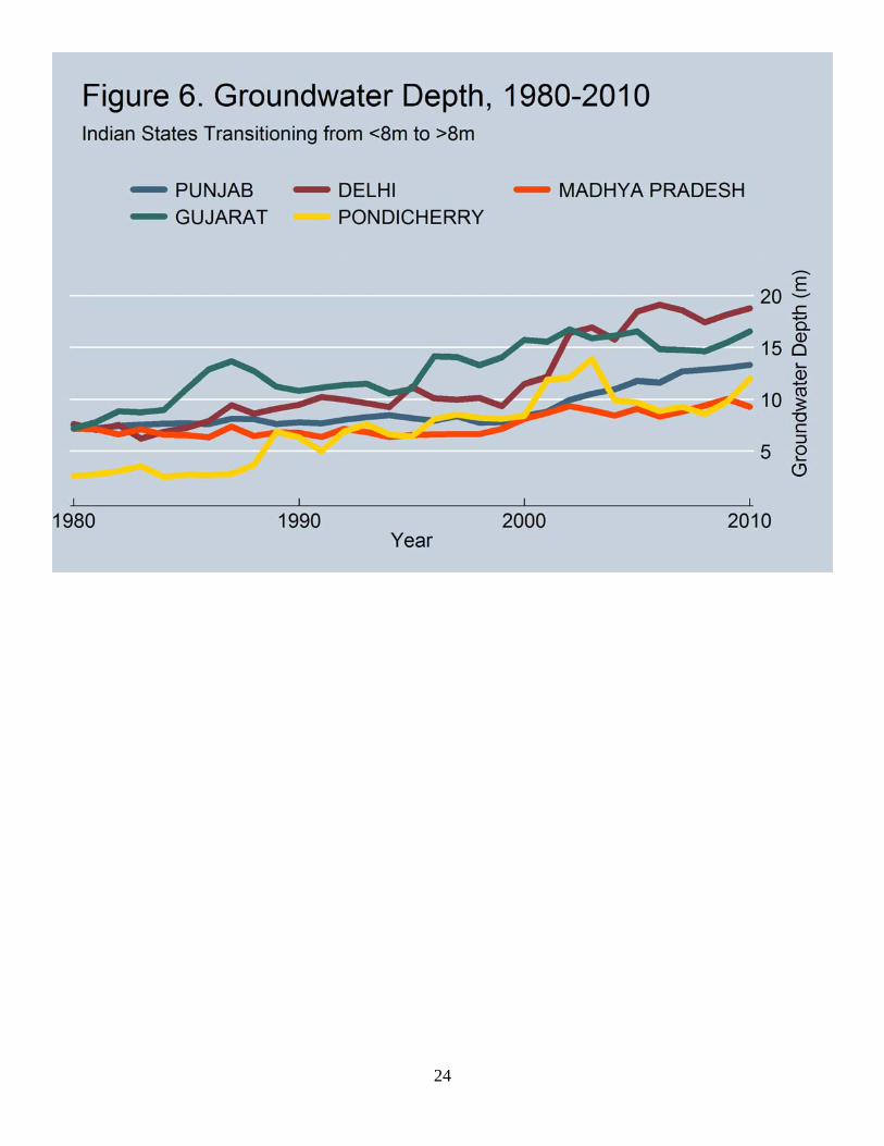
The cost of extracting groundwater depends on the depth of water table. There is a sharp

rise in the fixed cost of extracting groundwater at around 8 meters. At 8 meters, surface pumps

become infeasible to extract water and farmers have to invest in more expensive technologies

such as submersible pumps to extract groundwater.1 From social and economic perspective, it

becomes important to determine the extent of depletion where water tables fall from over 8

meters to below 8 meters. Figure 5 shows the districts where water table has fallen below 8

meters between 1980 and 2010. Most districts in Punjab have experienced such patterns of

decline. Other states including Haryana, New Delhi, Gujarat, Rajasthan, Madhaya Pradesh,

Maharashtra, Uttar Pradesh, Bihar, Jharkhand, West Bengal, Andra Pradesh, Pondicherry,

Kerala, and Tamil Nadu also have pockets where declines of water table are costly to the

farmers. Figure 6 shows the trends over time in the top 5 states -Punjab, Gujarat, Delhi,

Pondechery and Madhya Pradhesh - where average groundwater depth went from above 8 meters

to below 8 meters. Figure 7 shows the area of the states that experienced decline from above 8 to

below 8 meters. Punjab had the largest area experiencing such decline, followed by Pondicherry,

Madhya Pradesh, Haryana, New Delhi and Gujarat.

Three important facts emerge from these figures. One, the decline in water tables in India

is spatially heterogeneous with North Western region affected the most.2 Two, the bread basket

states, including Punjab and Haryana with endowments of thick aquifers are experiencing

significant declines in water tables. These states are the role models of green revolution. Three,

the decline has accelerated over time.

1 Surface pumps use atmospheric pressure to draw water. Atmospheric pressure can practically support the weight of a column of water of height 8 meters. 2 This is consistent with other findings using recent satellite based data. Data from NASA's GRACE satellites shows significant depletion of groundwater levels in Northern India. Non-renewable aquifers are being mined over large areas (NASA, 2009).

4

3 Why is Conservation Vital? Poverty and other Implications

From welfare perspective, rapid decline in water tables can result in significant social cost. Case

studies have documented that access to groundwater can reduce poverty and ensure food security

(Moench, 2001; Moench, 2003; Mookherji, 2008). Sekhri (2011a) uses groundwater data in

conjunction with annual agricultural output data at the district level to show that a 1 meter

decline in groundwater from its long term mean can reduce food grain production by around 8

percent. Controlling for district fixed effects, year fixed effects, and district specific trends, this

paper uses the plausibly exogenous fluctuations in groundwater depth from long term means to

estimate the effect of groundwater scarcity on food grain production. A 1 meter decline of

groundwater depth results in very large reduction in food grain production. Given that

groundwater irrigation is the main stay of irrigation in India, this is not unexpected. Consistent

with previous field studies, this paper shows that groundwater depletion can have significant

effect on food security in the country.

Sekhri (2012) identifies the causal impact of groundwater scarcity on poverty. Using village

level data from Uttar Pradesh, and exploiting the fact that there is a non-linearity in cost required

to access groundwater at 8 meters, this study shows that poverty rate increases by around 11

percent as groundwater depth falls below 8 meters. The full sample estimation controls for other

village characteristics that may be correlated with poverty rate and hence, generate omitted

variable bias. These include geographical controls like rainfall and temperature; geological

controls like elevation and slope; demographic characteristics like population, literacy rate, total

female population; infrastructure including availability of schools, medical facilities, access to

electricity, distance to nearest town, village council expenditure on public goods, banking facility

and bus service. This study uses a regression discontinuity design for identification. Both

parametric and non-parametric techniques have been used to show that the results do not depend

on the estimation method. The study provides a variety of tests to substantiate the findings. This

study also shows that self- reported conflict over irrigation water increases substantially near the

cutoff. The findings echo the results of field studies. Groundwater scarcity increases poverty. On

the flip side, uncontrolled access can lead to very rapid depletion. Therefore, sustainable access

5

to groundwater is required to curb poverty in rural areas of the country. One limitation of this

study is that is provides a static estimate. How poverty dynamically evolves with groundwater

depletion is not well understood. More work is required to understand and estimate the optimal

level of depletion in the long term.

In Gujarat, where the water tables are falling almost at a rate of 3 meters a year, Narula et al

(2011) estimate that water savings of 30 percent can free up 2.7 billion units of electricity for

non-agricultural use. Department of Drinking Water Supply, Government of India estimates that

in 2010, approximately 15 percent of the total habitations in the country went from full coverage

of drinking water to partial coverage due to drying up of sources. These findings indicate that the

welfare costs of groundwater depletion are very large in magnitude, and thus groundwater

depletion warrants an appropriate policy response.

4 Policy Response

State governments have introduced policies with the objective to reverse these trends of rapidly

falling groundwater. One of the first policies that has been introduced across many states is

mandated rainwater harvesting. States opted into selecting various measures for mandating rain

water harvesting. These measures included construction of rain water harvesting structures on

the roofs of buildings which met specific size criterion. Delhi was the first to pass this mandate

in 2001. The other states that mandated rain water harvesting include Andhra Pradesh, Tamil

Nadu, Kerala, Madhya Pradesh, Rajasthan, Bihar and West Bengal. Table 1 provides details of

the mandates along with the dates on which the mandates were passed. In this paper, I conduct a

district level analysis to examine whether such mandates have had any short run impact on water

table decline.

I also examine the impact of a policy pursued by the Gujarat government that promoted

decentralized rain water harvesting. Concentrated efforts to recharge groundwater began in the

Saurashtra region of Gujarat after the drought of 1987 (Mehta, 2006). Initial efforts to divert run-

off to groundwater wells led to widespread adoption of the practice by farmers throughout

Saurashtra without government intervention. Over time, farmers experimented with new

technologies and farmers began constructing check dams in streams and rivers to reduce water

6

speed and to allow the river water to seep into the ground and replenish the groundwater supply

(Mehta, 2006). Farmers continued constructing check dams through the 1990s with assistance

from NGOs who bore some of the costs.

In January, 2000, the Gujarat government introduced the Sardar Patel Participatory Water

Conservation Project in response to the work of farmers and NGOs in the Saurashtra, Kachchh,

Ahdamabad, and Sabar Kantha regions(Government of Gujarat, 2012b). The first phase of the

program ran from January 17, 2000 to February 20, 2001, and 10,257 check dams were

constructed by September 1, 2000. The program initially funded 60 percent of the estimated cost

of new check dams, and beneficiaries/NGOs financed the remaining 40 percent. By early 2004,

almost 24,500 check dams had been constructed, of which roughly 18,700 were in the Saurashtra

region (Pandya, 2004). In 2005, the government increased its financing to 80 percent of the

estimated cost, and the pace of construction increased outside of the Saurashtra region.

According to statistics from the Gujarat government, by the end of March, 2012 70,719 check

dams had been constructed in total under the project. Of these, 26,799 (38 percent) are in the

Saurashtra region, and 22,257 (31 percent) are in Kachchh or North Gujarat (Government of

Gujarat, 2012a). Figure 8 shows the geographic distribution of check dams constructed under the

Sardar Patel Participatory Water Conservation Project.

As discussed above, Punjab and Haryana are experiencing very rapid decline in water

tables. This can threaten future food security in the country. Punjab did not mandate rain water

harvesting. One of the key initiatives undertaken in Punjab to decelerate water table decline is

mandated delay of paddy transplanting. In 2006, the state government influenced the date of

paddy transplanting by changing the date on which free electricity is diverted to the farm sector

for operating mechanized tube wells for groundwater extraction. The date was pushed to June 10,

thereby reducing the amount of intensive watering that the crop can receive during its production

cycle (Tribune News service, 2006). The delayed date was mandated in 2008 via an ordinance.

This was later turned into a law -The Punjab Preservation of Sub Soil Water Act, 2009. The main

purpose of the law is to preserve groundwater by prohibiting sowing paddy before May 10 and

transplanting paddy before June 10. In addition, the law creates the authority to destroy, at the

farmer's expense, paddy sowed or transplanted early, and the law assesses a penalty of 10,000

rupees per month, per hectare of land in violation of the law (Government of Punjab, 2009).

7

Haryana followed suit and mandated delay in paddy transplanting in 2009. Haryana

passed its Preservation of Sub-Soil Water Act in March 2009, and it is very similar to the Punjab

act. Its main provisions prohibit sowing paddy before May 15 and transplanting paddy before

June 15. The law also contains punitive provisions similar to Punjab. These include destruction

of paddy sowed or transplanted early and a penalty of 10,000 rupees per month, per hectare of

land in violation of the law (Government of Haryana, 2009). The law took immediate effect for

the 2009 paddy season.3 In this paper, I make use of the timing of the introduction of this policy

in Punjab and Haryana to isolate the causal effect of the policy on water tables. Because of the de

facto prohibition of transplanting paddy before June 10 in Punjab, I treat 2006 as the effective

year for Punjab's policy rather than 2008.

4.1 Data Data from several sources has been combined to analyze the trends in Indian groundwater levels

since 1980, and to evaluate the impact of various policies on water table decline. The

groundwater level data are from the Indian Central Ground Water Board. Individual monitoring

well data has been used to construct measures of district groundwater depth from 1980 through

2010. The precipitation data from the University of Delaware Center for Climactic Research

have been used to calculate district annual average monthly precipitation through 2008. The

district precipitation data from the India Meteorological Department has been used for the years

2009 to 2010. In addition, district demographic and socioeconomic characteristics are from the

2001 Census of India. Area under various crops by districts is from the Directorate of Economics

and Statistics, Department of Agriculture and Cooperation, Ministry of Agriculture. This has

been used to classify districts as high rice growing districts as explained later.

4.1.1 Groundwater Data

The Indian Central Ground Water Board measures groundwater depth throughout each year at

approximately 16000 monitoring wells across India. In this paper, I use observations from 1980

to 2010 to construct district-level measures of groundwater depth. Groundwater depth is

3 Singh (2009) provides more details.

8

typically measured in January, May, August, and November although some wells have more or

fewer observations within a given year. The number of wells in the sample increased greatly over

the years. There were 3,305 wells in 1980, 11,063 in 1990, 15,782 in 2000, and 13,683 in 2010.

The density of wells in states increased to cover more geographical area and more states started

coverage. In the policy analysis conducted later, I use observations from year 2000 to 2010.

During this time, the number of wells was, by and large, stable. The monitoring wells are spread

over the entire country and not concentrated in any particular area. Wells have not been located

in places where the groundwater has been depleting the most. For these reasons, endogenous

well placement will not be a concern in the policy analysis.

In addition to groundwater depth, the data include latitude and longitude for each well, and I use

this information to match each well to the spatial boundaries of the Indian districts in 2001 and

construct a district-level panel of monthly and annual groundwater depth. These district-level

measures of groundwater levels are the primary outcomes studied in this paper.

4.1.2 Precipitation Data

I use precipitation data from the University of Delaware and the India Meteorological

Department to control for annual variation in precipitation which greatly affects groundwater

depth. The Center for Climactic Research at the University of Delaware compiled monthly

weather station data from 1900 to 2008 from several sources.4 From this data, all grid points

within India's administrative boundaries were extracted to construct district-level annual average

and monthly precipitation in each year. Since the Center for Climactic Research's data only cover

years through 2008, I use data from the India Meteorological Department for 2009 to 2010. The

India Meteorological Department collects monthly rainfall data for all Indian districts and

publishes tables for each district containing monthly rainfall for the past 5 years (India

4 These sources include the Global Historical Climatology Network, the Atmospheric Environment Service/Environment Canada, the Hydrometeorological Institute in St. Petersburg, Russia, GC-Net, the Automatic Weather Station Project, the National Center for Atmospheric Research, Sharon Nicholson's archive of African precipitation data, Webber and Willmott's (1998) South American monthly precipitation station records, and the Global Surface Summary of Day. After combining data from various sources, the Center for Climactic Research used various spatial interpolation and cross-validation methods to construct a global 0.5 degree by 0.5 degree latitude/longitude grid of monthly precipitation data from 1900 to 2008 (Matsuura and Wilmott, 2009).

9

Meteorological Department, 2012). For 2009 to 2010, district-level annual average and monthly

precipitation was calculated from these tables.

4.1.3 Demographic Data

The 2001 Indian census data has been used to control for district demographic and

socioeconomic characteristics. Specifically, district population, percent of the district population

with at least some college education, district literacy rate, district employment rate, and the

percent of the district population that is female have been controlled. Because these variables

have not been observed in intercensal years, these have been interacted with indicators for each

year in the sample to control for these characteristics non-parametrically in regression analysis.

4.1.4 Crop Production Data

Data on area under various crops by district has been used to construct high rice production and

low rice production district groups in the analysis of Punjab's and Haryana's policies to delay

paddy transplanting before the middle of June. Specifically, the fraction of cultivated area under

rice for each district in Punjab and Haryana has been calculated. I then classify districts in

Punjab and Haryana above the median as “high rice growing districts.”

4.2 Conceptual Framework

The change in the depth of groundwater is a function of demand side variables, supply side

variables, and natural recharge rate.

The change in depth can be modeled as: Wt-Wt-1 = Rt-Dt +St+ Et

Where Rt is the rate of recharge. This would be influenced by the geology of the place including

soil characteristics, slope, elevation and such features. These features are time invariant. The

recharge will also be affected by precipitation. Dt represents the demand side variables which

may include population, type of industry or sector that is dominant in the district, crops grown,

area under various crops, number of pumps being used, availability of alternate form of

irrigation, prices of crops, and inputs such as electricity and diesel. The supply side variables St

10

include management policies and prevalent institutions. Et represents an error term. Most of the

policies that have been designed change the factors in the set St. In what follows, I examine a

subset.

A few comments on relating this model to the policy analysis conducted are in order. I use panel

data and the methodologies used control for time invariant characteristics of districts. I also

control for rainfall and temperature in every regression to account for the recharge. I do not have

data on very comprehensive set of variables that can affect the demand for groundwater. I do

control for a set of demographic and economic variables. But to the extent that these variables

have not influenced policy choices or implementation logistics differentially in treated and

control areas, the estimation yields unbiased results.

The following analysis is carried out at the level of districts. Districts are administrative units

under states. Most program allocations and monitoring of government programs are delegated to

districts. Hence, they are a natural choice for unit of analysis. One concern may be that the

underlying aquifers are interconnected. The lateral velocity of groundwater is very low (Todd,

1980). Hence, over this time frame spatial externalities may not have arisen. I address this more

specifically in the analysis, where I allow spatial correlation between standard errors.

4.3 Identification Strategy Rain Water Harvesting Mandates The states selected into mandating rainwater harvesting. Hence, comparing the outcomes in the

states that mandated rain water harvesting with the ones that did not, will result in biased

estimates. Therefore, I compare groundwater levels in districts in the states that passed the

mandates earlier to the states that passed them later in order to circumvent selection concerns.

The identifying assumption is that the timing of such mandates is plausibly exogenous.

The empirical model is as follows:

∗ (1)

where is the groundwater level in district i in state s at time t, are the year fixed effects,

is the treatment indicator which takes the value 1 if the district is in a treated state, and is

a vector of time varying district specific controls. Post is an indicator variable that switches to 1

11

after the rain water harvesting mandates were passed in the states. The coefficient is the

parameter of interest. is the error term. Robust standard errors are clustered at the level of

states. Year specific common shocks to all districts are absorbed by the time fixed effects. Time

invariant district specific omitted variables that affect the likelihood of treatment are controlled

for by including the treatment indicator. The interaction ∗ yields the effect of the

treatment on the treated post treatment where the treatment is passing of rain water harvesting

mandates.

4.3.1 Decentralized Rain Water Harvesting – Sardar Patel Participatory

Water Conservation Project

I compare the groundwater levels of districts in the regions that received the subsidy program

earlier in January 2000 (treatment regions – Saurashtra, Kachchh, Ahdamabad, and Sabar Kantha

regions) to the districts that received the program later in 2005 when it expanded (control

regions).5 Figure 9 plots the average groundwater level in the treated and the control districts

from 1990 to 2011. The pretreatment groundwater levels prior to 2000 are similar across these

districts and the two groups do not exhibit differential trends. The following empirical model is

estimated using the data from 1990 to 2011:

∗ (2)

where is the groundwater level in district d in region r at time t, are the year fixed effects,

is the treatment indicator which takes the value 1 if the district is in a treated region, and

is a vector of time varying district specific controls. Post is an indicator variable that switches to

1 after 1999. The coefficient is the parameter of interest. is the error term. Robust

standard errors are clustered at the level of districts. Year specific common shocks to all districts

are absorbed by the time fixed effects. Time invariant district specific omitted variables that

affect the likelihood of treatment are controlled for by including the treatment indicator. Region

specific time invariant unobservables are absorbed by the region fixed effects in certain

specifications. It is important to note that the areas where the subsidy was initiated first were the

5 Districts in treated group include Rajkot, Junagadh, Bhavnagar, Porbandar, Jamnagar, Amreli, Surendranagar, Ahmadabad, Kachchh, and Sabar Kantha. Control group includes Banas Kantha, Patan, Mahesana, Gandhinagar, Kheda, Anand, Panch Mahals, Dohad, Valdora, Narmada, Bharuch, Surat, Navsari, the Dangs, and Valsad.

12

ones where such decentralized initiatives were successful with the help of NGOs and donor

funding. Hence, the estimated coefficient cannot be interpreted as causal. Although pretrends in

groundwater level are controlled for, there can be other potential time varying factors that

influenced early initiation of the program and are unobserved. An example could be a gradual

change in people's attitude towards groundwater conservation or awareness about implications of

water depletion.

4.3.2 Delayed Paddy Transplanting

In the estimation procedure, I employ a difference-in-difference methodology comparing the

paddy growing areas in Punjab to the bordering Haryana. Since both states adopted measures to

ensure delayed transplanting of paddy at different time, I use the variation in the timing of

introduction of the policy to evaluate its impact on groundwater levels. As mentioned before, in

Punjab, the de-facto change in date of transplanting happened in 2006 and in Haryana, the

mandate was passed in 2009. The rice growing districts were identified using the area under

various crops. The districts where the ratio of area under rice to the total cultivated area exceeded

the sample median in 2003 for all districts in Haryana and Punjab are considered the high rice

growing districts. Since the policy delayed transplanting rice, the policy should have affected the

water use in rice growing districts, and hence impact water tables in these districts. Figure 10

maps the high rice production districts (treatment) and low rice production districts (control) in

Punjab and Haryana.6 I compare the high rice growing districts with low rice growing districts

before and after the policy change.

The empirical specification is given by:

∗ ∗ ∗

(3)

where is the groundwater level in district i at time t. are the year fixed effects, is an

indicator variable which takes value 1 if the district is rice growing district and 0 otherwise, and

is a vector of time varying district specific controls. Post is an indicator variable that

6 High rice production districts are Gurdaspur, Amritsar, Firzopur, Faridkot, Moga, Kapurthala, Jalandhar, Nawanshahr, Ludhiana, Sangrur, Fatehgarh Sahbi, Patala, Kaithal, Kurukshetra, Ambala, Yamunanagar, Karnal, and Panipat. The low rice production districts are Hoshiapur, Rupnagar, Muktsar, Bathinda, Mansa, Panchkula, Sirsa, Fatehabad, Hisar, Jind, Sonipat, Rohtak, Bhiwani, Jhajjar, Manendragarh, Rewari, Gurgagon, and Faridabad.

13

switches to 1 after the paddy transplanting was delayed and is equal to 0 before that. The

coefficient is the parameter of interest. The regressions include full sets of interaction

between state and rice growing districts, and rice growing districts and year indicators. is the

error term. Robust standard errors are clustered at the level of districts. I also report Conley

(1999) errors to account for spatial correlation in groundwater levels of neighboring districts.7

Year specific common shocks to all districts are absorbed by the time fixed effects. Time

invariant rice growing district specific omitted variables are controlled for by including the rice

growing indicator. The specifications allow for high rice growing districts in the two states to be

different by including state times rice growing fixed effects. Differences in high rice growing

and low rice growing districts over years are also accounted for by including high rice growing

districts times year fixed effects. The vector includes average annual rainfall in the district

and demographic controls including percentage of females, percentage of working population,

percentage of literate population, percentage of population with some college, and total

population.8 The interaction term ∗ yields the difference-in-difference estimator. In

robustness checks, I also allow for state specific trends that non-parametrically account for time

varying state specific factors that may have influenced timing of treatment.

4.3.3 Results

Tables 2 and 3 report the results for the impact of rain water harvesting mandates on

groundwater levels. Table 2 reports the effect on groundwater levels for 4 different months-

January, May, August, and November. Each specification includes treatment and year fixed

effects. I do not find evidence of beneficial effects of rainwater harvesting mandates on

groundwater levels at least in the short run. The coefficients on the interaction term are

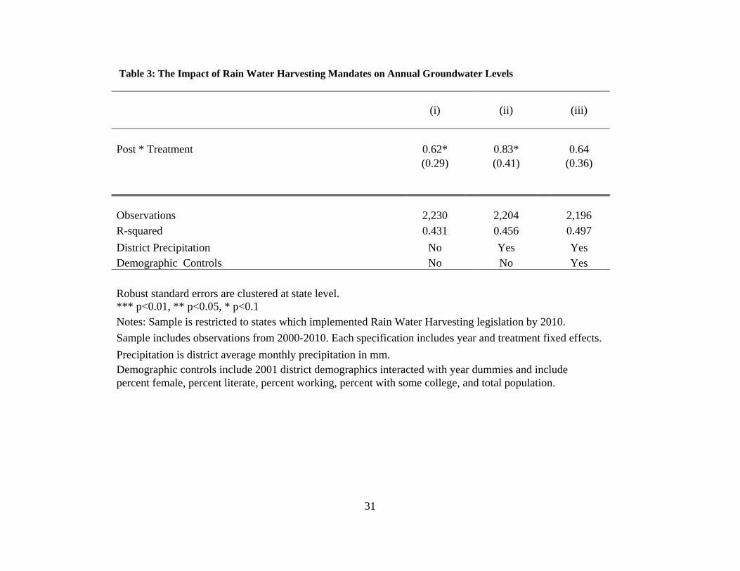
statistically insignificant.9 In Table 3, this analysis is repeated for annual groundwater levels.

Each specification controls for state and year fixed effects. In column (ii), annual average district

precipitation is added to the empirical specification and in column (iii), demographic controls

interacted with year indicators are added in addition to the precipitation. Although, the

7 The aquifers could be interconnected. The lateral velocity of groundwater is very low. In the short run, cross district externalities are not likely to arise. Conley's standard errors correct for such externalities. 8 These variables are available for the year 2001 from the Census of India. These are interacted with year indicators to control for trends in these variables starting at the 2001 initial values. 9 The number of observations change across specifications because of missing data in some of the district year cells.

14

interaction term is marginally significant at 10 percent in the columns (i) and (ii), this is not

robust to including demographic controls in column (iii). These results do not bear out any

evidence of a beneficial effect of rain water harvesting mandates on water tables in the short run.

Table 4 reports the results for the impact of the Sardar Patel Participatory Water

Conservation Project on annual groundwater levels. The subsidy program had an ameliorative

effect on groundwater levels. Column (i) reports the baseline specification. The coefficient is

negative but statistically insignificant. In column (ii), I add region fixed effects. Columns (iii)

and (iv) control for annual precipitation levels with and without region fixed effects. The effect

continues to be statistically insignificant. In columns (v) and (vi), demographic controls are

added interacted with year indicators are added in addition to the precipitation. Both

specifications -with and without region fixed effects- yield a negative and highly statistically

significant effect of the program. The point estimate of 9.3 is 0.82 of a standard deviation and

very large in magnitude. The subsidy program had a huge effect on the annual groundwater level

in treated areas. However, these results should be interpreted with caution as the areas that

received the early treatment were the areas where decentralized rain water harvesting was very

effective prior to the subsidy program. The government focused the subsidy in regions where

NGOs and other donor funded projects were successful. Hence, I cannot rule out selection bias.

As mentioned before, previous experience with such projects may have gradually changed the

attitudes towards conservation which is unobserved. Controlling demographic characteristics in

column (v) of Table 4 relative to column (iv) changes the results substantially. This strongly

suggests that program was targeted selectively in certain types of areas. Figure 9 shows that

there are no differential trends in groundwater level prior to the program. Hence, it is likely that

the results emerge as a result of this program alone. On the other hand, it is possible that such

programs may not be successful in randomly chosen areas, where people do not have prior

experience with such projects. More research is required to address selection and establish the

causal impact of such subsidy programs.

Tables 5 and 6 report the results of the impact of delayed paddy transplantation on

groundwater levels. The outcome variable is depth to groundwater in meters below ground level

(mbgl). Paddy transplantation occurs in June. Table 5 reports the effect of the policy on post

transplanting groundwater level in August and Table 6 reports the results for annual depth to

groundwater. Column (i) in Table 5 shows the coefficient of the interaction term from a

15

specification which includes year fixed effects, state X rice fixed effects, and rice X year fixed

effects. In column (ii), precipitation is added to the regression specification. Column (iii) controls

for trends in demographic variables, and column (iv) includes state specific time trends in

addition to the above mentioned controls. In all specifications, the policy increases depth to

groundwater. The coefficient is marginally significant at 10 percent significance level is the most

conservative specification in column (iv). The August groundwater levels declined in response to

the policy. The depth to groundwater level in high rice growing districts post the policy change

was 1.17 meters deeper than the low rice growing districts. Similar specifications are repeated

for the annual depth to groundwater in Table 6. In each specification, the coefficient on the

interaction term is positive and highly statistically significant. In the last column, we observe a

decline in depth of 1.60 mbgl and it is significant at 1 percent level. This effect is 0.28 of a

standard deviation and is economically moderate. The findings indicate that the annual

groundwater level situation worsened in rice growing areas after the policy change.10 It is

possible that the farmers responded to the policy by increasing the number of irrigations applied

or using more water per irrigation after the mid June transplanting.11

5. What do we learn from the experience with these policies?

The rain water harvesting mandates were unsuccessful in reversing the depletion rates whereas

the decentralized experience in Gujarat has been more positive. From this comparison it appears

that technical or engineering limitations or short duration that has elapsed since the program

commencement are not the principal explanations for success or failure of these policies. The

effective policies will need to be decentralized in nature. Engagement of the stake holders is an

important ingredient for these policies to work. Bottom-up rather than top-down policy tools are

more successful. None of these policies are pricing mechanisms. In Sekhri (2011b), I show that

public wells provision can reduce the rate of depletion. If an optimal price is charged it can also

reverse depletion. But this can work only where cost of groundwater extraction is high, or in

other words in areas where water tables are deep. In Sekhri and Foster (2008), we find evidence

10 In contrast to these findings, Singh(2009) estimates a 30 cm water saving effect of the policy but the estimate is based on simulations using historic data from central Punjab and does not account for selection issues. 11 In the absence of farm level data on applied number of irrigations and water use, it is not possible to establish the mechanism.

16

that bilateral trade arrangements between farmers who sell and buy groundwater also decelerate

depletion rates. The benefit of promoting these is that these arrangements do not require top

down monitoring. Introduction of pricing mechanisms may be another important lever to reduce

over-extraction.

6. Future Directions with Policy Choices

What kind of policies- direct or indirect- can or cannot work? Reducing electricity subsidies can

potentially affect groundwater extraction rates (Badiani and Jessoe, 2011). West Bengal and

Uttarakhand have recently adopted metering of electricity for tube wells. Gujarat, under the

flagship Jyotirgram Yojana, has separated agricultural feeders from non-agricultural feeders,

improved the quality of the power supply and rationed the number of hours of electricity to

agriculture to 8 hours a day. Important policy lessons can be learnt from the experience of these

states.12 Other possibilities include promoting water saving infrastructure and agricultural

practices. More research is required to understand the effect of policies that promote such

practices, and is a very promising area of future research.

12 Mukherji et al (2010) provide details of the reforms.

17

Bibliography

Agriculture Census Division, Ministry of Agriculture, Governemnt of India. (2006). Agricultural Census of India Database.

Badiani, R., & Jessoe, K. K. (2011). Electricity subsidies for agriculture: Evaluating the impact and persistence of these subsidies in India. University of California Davis Working Paper.

Conley, T. G. (1999). GMM Estimation with Cross Sectional Dependence. Journal of Econometrics, 92(1), 1-45.

FAO ( 2012) AQUASTAT database - Food and Agriculture Organization of the United Nations (FAO). Website accessed on [05/12/2012 5:42] Foster, A., & Sekhri, S. (2008). Can Expansion of Markets for Groundwater in Rural India?

Brown University Working Paper. Government of Gujarat. (2012a). Details of Checkdams Completed in Gujarat State as on 31

March 2012. Retrieved from http://www.guj-nwrws.gujarat.gov.in/showpage.aspx?contentid=1537&lang=English

Government of Gujarat. (2012b). Sardar Patel Participatory Water Conservation Scheme - Water Conservation through Partnership Between People and Government - Success Story Of Gujarat. Retrieved from http://www.guj-nwrws.gujarat.gov.in/showpage.aspx?contentid=1538&lang=English

Haryana Government. (2009, March 18). The Haryan Preservation of Sub-Soil Water Act. India Meteorological Department. (2012). Last 5-Years Districtwise Rainfall. Retrieved from

http://www.imd.gov.in/section/hydro/distrainfall/districtrain.html Kelbert, A., Schultz, A., & Egbert, G. (2008). Global Electromagnetic Induction Constraints on

Transition-zone Water Content Variations. Nature. Kumar, B. (2007, July 31). Punjab's Depleting Groundwater Stagnates Agricultural Growth.

Retrieved from DownToEarth: http://www.downtoearth.org.in/node/6267 Matsuura, K., & Willmott, C. J. (2009). Terrestrial Precipitation: 1900-2008 Gridded Monthly

Time Series. Version 2.01. Center for Climactic Research at University of Delaware. Retrieved from http://climate.geog.udel.edu/~climate/html_pages/download.html

Mehta, A. (2006). The Rain Catchers of Saurashtra, Gujarat. In K. Okonski (Ed.), The Water Revolution: Practical Solutions to Water Scarcity (p. 226). London: International Policy Press.

Modi, V., Kapil, N., Fishman, R., & Polycarpou, L. (2011). Addressing the Water. Columbia Water Center White Paper.

Moench, M. (2003). “Groundwater and Poverty: Exploring the Connections”, In Llamas, R. and Custodio, E. (eds.). Intensive Use of Groundwater: Challenges and Opportunities, Swets & Zeitlinger B.V., Lisse, The Netherlands, pp. 441–455 Mukherji, A. (2008), "Poverty, groundwater, electricity and agrarian politics: Understanding the linkages in West Bengal" Mukherji, A., Shah, T., & Verma, S. (2010). Electricity reforms and their impact on ground

water use in states of Gujarat, West Bengal and Uttarakhand, India. In J. Lundqvist (Ed.), On the Water Front: Selections from the 2009 World Water Week in Stockholm. Stockholm: Stockholm International Water Institute.

18

National Sample Survey Office. (2011). Key Indicators of Employment and Unemployment in India, 2009-2010.

One India News. (2008, June 11). Power Situation Normal in Punjab as Paddy Sowing Begins. Retrieved from One India News: http://news.oneindia.in/2008/06/09/power-situation-normal-in-punjab-as-paddy-sowing-begins-1213167693.html

Pandya, H. (2004, February 24). Check Dams Help Raise Water Table in Jamnagar, Amreli. Business Standard. Retrieved from http://www.business-standard.com/india/news/check-dams-help-raise-water-table-in-jamnagar-amreli/145167/

Parkash, C. (2006, April 29). Power Supply to Improve from May 1. Tribune India. Retrieved from Tribune India: http://www.tribuneindia.com/2006/20060429/punjab1.htm

Punjab Government. (2009, April 28). The Punjab Preservation of Sub Soil Water Preservation Act.

Punjab Newsline. (2006, June 13). PSEB Copes with High Demand of Power for Paddy. Retrieved from Punjab Newsline: http://punjabnewsline.com/content/view/698/70

Registrar General and Census Commissioner, India. (2001). Census of India. Repeto, R. (1994), `The Second India' Revisited:popultaion, poverty and environmental stress

over two decades, Washington,DC, World Resources Institute. Sekhri, S. (2011a). Missing Water: Agricultural Stress and Adaptation Strategies in. Mimeo,

University of Virginia. Sekhri, S. (2011b). Public Provision and Protection of Natural Resources: Groundwater.

American Economic Journal: Applied Economics, 3(4), 29-55. Sekhri, S. (2012). Wells, Water and Welfare: Impact of Access to Groundwater on Rural

Poverty. Mimeo, University of Virginia. Shah, T., Scott, C., Kishore, A., & Sharma, A. "Energy-Irrigation Nexus in South Asia: Improving groundwater Conservation and Power Sector Viability" , Chapter 11 in The Agricultural Groundwater Revolution: Opportunities and Threat to Development, ed. M. Giordana and K.G. Villholth, 2007, CAB International Shankar, P. V., Kulkarni, H., & Krishnan, S. (2011). India's Groundwater Challenge and the

Way Forward. Economic and Political Weekly, 46(2). Singh Gill, P. P. (2006, April 11). Punjab Advances Power Austerity Drive. Retrieved from

Business Standard: http://www.business-standard.com/india/news/punjab-advances-power-austerity-drive-date/239859/

Singh, K. (2009). Act to Save Groundwater in Punjab: Its Impact on Water Table, Electricity Subsidy and Environment. Agricultural Economics Research Review, 365-386.

Todd, D. 1980 Groundwater hydrology, John Wiley & Sons Tribune News Service. (2006, June 13). Power Woes Return with Paddy Season. Tribune India.

Retrieved from http://www.tribuneindia.com/2006/20060613/punjab1.htm#12 Webber, S. R., & Willmott, C. J. (1998). South American Precipitation: 1960-1990 Gridded

Monthly Time Series (Version 1.02). Newark, Delaware: Center for Climatic Research, Deptartment of Geography, University of Delaware.

19

20

Figure 2. Decadal Changes in Indian District Groundwater Depth

21

Figure 3. District Groundwater Depth in Selected States, 1980-2010

22

23

24

25

26

27

28

29

Table 1: Rain Water Harvesting Mandates

State Year Passed Description Delhi 2001 RWH mandatory for all new buildings with more than 100 sq m roof area and all newly

developed plots of land larger than 1000 sq m. Also,mandated RWH by March 31, 2002 for all institutions and residential colonies in notified areas (South and southwest Delhi, and adjoining areas) and all buildings in notified areas that have tubewells

Andhra Pradesh

2002 Andhra Pradesh Water, Land and Tree Act, 2002 stipulates mandatory provision to construct RWH structures at new and existing constructions for all residential, commercial and other premises and open space having area of not less than 200 sq m in the stipulated period, failing which the authority construct such RWH structures and recover the cost incurred along a prescribed penalty

Tamil Nadu 2003 Vide Ordinance No. 4 of 2003 dated July, 2003 mandates RWH facilities for all existing and new buildings. Like Andhra Pradesh, the state may construct RWH facilities and recover the cost incurred by means of property taxes

Kerala 2004 Roof top RWH is mandatory for all new buildings as per Kerala Municipality Building (Amendment) Rules, 2004

Madhya Pradesh

2006 The State Govt. vide Gazette notification dated 26.8.2006, has made roof top RWH mandatory for all buildings with plot size larger than 140 sq.m. Also there is a 6% rebate in property tax to individuals for the year in which the individual installs roof top RWH structures.

Rajasthan 2006 Roof Top RWH is mandatory in state-owned buildings and all buildings with plots larger than 500 sq m in urban areas

Bihar 2007 The Bihar Ground Water Act, enacted in 2007, mandates privions of RWH structures for buildings with plots larger than 1000 sq m

West Bengal 2007 Vide Rule 171 of the West Bengal Municipal (Building) Rules, 2007, mandates installation of RWH system on new and existing buildings

Sources: http://www.rainwaterharvesting.org/Policy/Legislation.htm#

State profiles at: http://cgwb.gov.in/gw_profiles/st_ap.htm http://www.cseindia.org/content/legislation-rainwater-harvesting

30

Table 2: The Impact of Rain Water Harvesting Mandates on Seasonal Groundwater Levels

(i) (ii) (iii) (iv) January May August November

Post * Treatment 0.84* 0.86* 0.51 0.35

(0.44) (0.37) (0.42) (0.24)

Observations 2,206 2,153 2,060 2,118 R-squared 0.435 0.433 0.405 0.433

Robust standard errors are clustered at the state level. *** p<0.01, ** p<0.05, * p<0.1 Notes: Sample is restricted to states which implemented Rain Water Harvesting legislation by 2010. Sample includes observations from 2000-2010. Each specification includes year and treatment fixed effects.

31

Table 3: The Impact of Rain Water Harvesting Mandates on Annual Groundwater Levels

(i) (ii) (iii)

Post * Treatment 0.62* 0.83* 0.64 (0.29) (0.41) (0.36)

Observations 2,230 2,204 2,196 R-squared 0.431 0.456 0.497

District Precipitation No Yes Yes Demographic Controls No No Yes

Robust standard errors are clustered at state level. *** p<0.01, ** p<0.05, * p<0.1 Notes: Sample is restricted to states which implemented Rain Water Harvesting legislation by 2010.

Sample includes observations from 2000-2010. Each specification includes year and treatment fixed effects.

Precipitation is district average monthly precipitation in mm. Demographic controls include 2001 district demographics interacted with year dummies and include percent female, percent literate, percent working, percent with some college, and total population.

32

Table 4: The Impact of Sardar Patel Water Conservation Subsidy Program on Annual Groundwater Level

(i) (ii) (iii) (iv) (v) (vi)

Treatment x Post-1999 -4.744 -4.744 -3.742 -4.593 -9.318*** -9.314***

(2.918) (2.932) (2.661) (2.974) (1.540) (1.593) [2.847] [2.847] [2.586] [2.882] [1.309] [1.347]

Observations 550 550 550 550 550 550 R-squared 0.056 0.597 0.249 0.598 0.762 0.810 Year FE YES YES YES YES YES YES Treatment FE YES YES YES YES YES YES Region FE NO YES NO YES NO YES Precipitation (mm) NO NO YES YES YES YES Census Controls NO NO NO NO YES YES Robust standard errors clustered at district level are in parenthesis and Conley (1999) standard errors correcting for spatial correlation are in brackets. *** p<0.01, ** p<0.05, * p<0.1 Note: Sample restricted to districts in Gujarat and includes observations from 1990-2011. All regressions include a Treatment dummy for districts which received early check dam construction from the Sardar Patel Participatory Water Conservation Program. These include the Saurasthra region, Kachchh, Ahdamabad, and Sabar Kantha. Regions in Gujarat include Kachchh, North Gujarat, Central Gujarat, Saurashtra, East Gujarat, and South Gujarat. Precipitation is district average monthly precipitation in mm. Census controls include 2001 district demographics interacted with year dummies and include percent female, percent literate, percent working, percent with some college, and total population.

33

Table 5: The Impact of Delay in Paddy Transplantation on Groundwater Levels Post Transplanting

(Groundwater Level Measured in August)

(i) (ii) (iii) (iv)

Post * High Rice Producing Districts 1.30** 1.28** 1.13 1.17*

(0.53) (0.53) (0.70) (0.64) [0.51] [0.51] [0.62] [0.57]

Observations 324 321 321 321 R-squared 0.100 0.101 0.252 0.254 State x Rice FE Yes Yes Yes Yes Year x Rice FE Yes Yes Yes Yes District Precipitation No Yes Yes Yes Census Controls No No Yes Yes State Specific Time Trend No No No Yes Robust standard errors clustered at district level are in parentheses. Conley (1999) standard errors correcting for spatial correlation are in brackets. *** p<0.01, ** p<0.05, * p<0.1 Note: Sample is restricted to districts in Punjab and Haryana. Each regression controls for year fixed effects Sample includes observations from 2003-2011. Districts with rice area as a fraction of total cultivated area above the median in Punjab and Haryana (.30) are classified as rice-producing. Punjab began limiting paddy water supply in 2006 (2 years before its legislation) by way of rationing electricity, and Haryana passed legislation in 2009. Precipitation is district average monthly precipitation in mm. Census controls include 2001 district demographics interacted with year dummies and include percent female, percent literate, percent working, percent with some college, and total population.

34

  Table 6: The Impact of Delay in Paddy Transplantation on Annual Groundwater Levels

(i) (ii) (iii) (iv)

Post * High Rice Producing Districts 1.25*** 1.13** 1.58*** 1.60***

(0.45) (0.46) (0.54) (0.53) [0.44] [0.45] [0.48] [0.47]

Observations 324 321 321 321 R-squared 0.090 0.097 0.248 0.249 State x Rice FE Yes Yes Yes Yes Year x Rice FE Yes Yes Yes Yes District Precipitation No Yes Yes Yes Census Controls No No Yes Yes State Specific Time Trend No No No Yes Robust standard errors clustered at district level are in parentheses. Conley (1999) standard errors correcting for spatial correlation are in brackets. *** p<0.01, ** p<0.05, * p<0.1 Note: Sample is restricted to districts in Punjab and Haryana. Each regression controls for year fixed effects Sample includes observations from 2003-2011. Districts with rice area as a fraction of total cultivated area above the median in Punjab and Haryana (.30) are classified as rice-producing. Punjab began limiting paddy water supply in 2006 (2 years before its legislation) by way of rationing electricity, and Haryana passed legislation in 2009. Precipitation is district average monthly precipitation in mm. Census controls include 2001 district demographics interacted with year dummies and include percent female, percent literate, percent working, percent with some college, and total population.