tbs910 regression models

Regression ModelsRegression ModelsRegression ModelsRegression Models

TBS910 BUSINESS ANALYTICSTBS910 BUSINESS ANALYTICS

byProf. Stephen Ong

Visiting Professor, Shenzhen University

Visiting Fellow, Sydney Business School, University of Wollongong

Today’s Overview Today’s Overview

Learning ObjectivesLearning Objectives

1.1. Identify variables and use them in a regression model.Identify variables and use them in a regression model.2.2. Develop simple linear regression equations. from sample data and Develop simple linear regression equations. from sample data and

interpret the slope and intercept.interpret the slope and intercept.3.3. Compute the coefficient of determination and the coefficient of Compute the coefficient of determination and the coefficient of

correlation and interpret their meanings.correlation and interpret their meanings.4.4. Interpret the Interpret the FF-test in a linear regression model.-test in a linear regression model.5.5. List the assumptions used in regression and use residual plots to List the assumptions used in regression and use residual plots to

identify problems.identify problems.6.6. Develop a multiple regression model and use it for prediction Develop a multiple regression model and use it for prediction

purposes.purposes.7.7. Use dummy variables to model categorical data.Use dummy variables to model categorical data.8.8. Determine which variables should be included in a multiple Determine which variables should be included in a multiple

regression model.regression model.9.9. Transform a nonlinear function into a linear one for use in regression.Transform a nonlinear function into a linear one for use in regression.10.10. Understand and avoid common mistakes made in the use of Understand and avoid common mistakes made in the use of

regression analysis.regression analysis.

After completing this lecture, students will be able to:After completing this lecture, students will be able to:

Regression Models : OutlineRegression Models : Outline4.14.1 IntroductionIntroduction4.24.2 Scatter DiagramsScatter Diagrams4.34.3 Simple Linear RegressionSimple Linear Regression4.44.4 Measuring the Fit of the Regression ModelMeasuring the Fit of the Regression Model4.54.5 Using Computer Software for RegressionUsing Computer Software for Regression4.64.6 Assumptions of the Regression ModelAssumptions of the Regression Model4.74.7 Testing the Model for SignificanceTesting the Model for Significance4.84.8 Multiple Regression AnalysisMultiple Regression Analysis4.94.9 Binary or Dummy VariablesBinary or Dummy Variables4.104.10 Model BuildingModel Building4.114.11 Nonlinear Regression Nonlinear Regression 4.124.12 Cautions and Pitfalls in Regression AnalysisCautions and Pitfalls in Regression Analysis

5-5

Regression Regression AnalysisAnalysis

MultipleMultiple

RegressionRegression

MovingAverage

Exponential Smoothing

Trend Projections

Decomposition

Delphi Methods

Jury of Executive Opinion

Sales ForceComposite

Consumer Market Survey

Time-Series Time-Series MethodsMethods

Qualitative Qualitative ModelsModels

Causal Causal MethodsMethods

Forecasting ModelsForecasting ModelsForecasting Forecasting TechniquesTechniques

Figure 5.1

IntroductionIntroduction

Regression analysisRegression analysis is a very valuable tool is a very valuable tool for a manager.for a manager.

Regression can be used to:Regression can be used to: Understand the relationship between variables.Understand the relationship between variables. Predict the value of one variable based on Predict the value of one variable based on

another variable.another variable.

Simple linear regression models have only Simple linear regression models have only two variables.two variables.

Multiple regression models have more Multiple regression models have more variables.variables.

IntroductionIntroduction The variable to be predicted is called The variable to be predicted is called

the the dependent variabledependent variable.. This is sometimes called the This is sometimes called the response response

variable.variable.

The value of this variable depends on The value of this variable depends on the value of the the value of the independent variable.independent variable. This is sometimes called the This is sometimes called the explanatoryexplanatory

or or predictor variable.predictor variable.

Independent Independent variablevariable

Dependent Dependent variablevariable

Independent Independent variablevariable

= +

4-8

Scatter DiagramScatter Diagram A A scatter diagramscatter diagram or or scatter plotscatter plot

is often used to investigate the is often used to investigate the relationship between variables.relationship between variables.

The independent variable is The independent variable is normally plotted on the normally plotted on the XX axis. axis.

The dependent variable is The dependent variable is normally plotted on the normally plotted on the YY axis. axis.

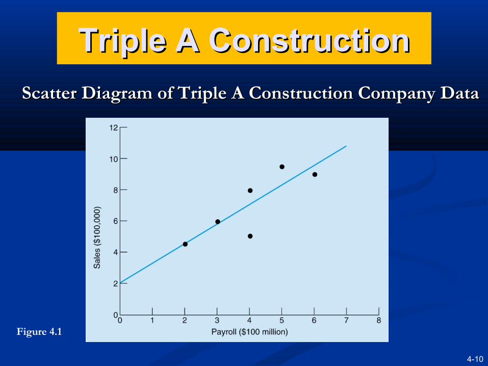
Triple A ConstructionTriple A Construction Triple A Construction renovates old homes.Triple A Construction renovates old homes. Managers have found that the dollar volume Managers have found that the dollar volume

of renovation work is dependent on the area of renovation work is dependent on the area payroll.payroll.

TRIPLE A’S TRIPLE A’S SALESSALES

($100,000s)($100,000s)

LOCAL PAYROLLLOCAL PAYROLL($100,000,000s)($100,000,000s)

66 33

88 44

99 66

55 44

4.54.5 22

9.59.5 55Table 4.1

4-10

Triple A ConstructionTriple A Construction

Figure 4.1

Scatter Diagram of Triple A Construction Company DataScatter Diagram of Triple A Construction Company Data

Simple Linear RegressionSimple Linear Regression

wherewhereYY = dependent variable (response)= dependent variable (response)

XX = independent variable (predictor or explanatory)= independent variable (predictor or explanatory) ββ 00 = intercept (value of = intercept (value of YY when when XX = 0) = 0)

ββ 11 = slope of the regression line = slope of the regression line

εε = random error= random error

Regression models Regression models are used to test if there is are used to test if there is a relationship between variables.a relationship between variables.

There is some There is some random error random error that cannot be that cannot be predicted.predicted.

εββ ++= XY 10

Simple Linear RegressionSimple Linear Regression True values for the slope and intercept True values for the slope and intercept

are not known so they are estimated are not known so they are estimated using sample data.using sample data.

XbbY 10 +=ˆwherewhere

YY = predicted value of = predicted value of YYbb00 = estimate of = estimate of ββ00, based on sample results, based on sample results

bb11 = estimate of = estimate of ββ11, based on sample results, based on sample results

^


Triple A Construction is trying to Triple A Construction is trying to predict sales based on area payroll.predict sales based on area payroll.

YY = Sales = SalesXX = Area payroll = Area payroll

The line chosen in Figure 4.1 is the one The line chosen in Figure 4.1 is the one that minimizes the errors.that minimizes the errors.

Error = (Actual value) – (Predicted value)Error = (Actual value) – (Predicted value)

YYe ˆ−=

Triple A ConstructionTriple A ConstructionFor the simple linear regression model, the For the simple linear regression model, the values of the intercept and slope can be values of the intercept and slope can be calculated using the formulas below.calculated using the formulas below.

XbbY 10 +=ˆ

values of (mean) average Xn

XX == ∑

values of (mean) average Yn

YY == ∑

∑∑

−−−

= 21 )(

))((

XX

YYXXb

XbYb 10 −=


YY XX ((XX – – XX))22 ((XX – – XX)()(YY – – YY))

66 33 (3 – 4)(3 – 4)22 = 1 = 1 (3 – 4)(6 – 7) = 1(3 – 4)(6 – 7) = 1

88 44 (4 – 4)(4 – 4)22 = 0 = 0 (4 – 4)(8 – 7) = 0(4 – 4)(8 – 7) = 0

99 66 (6 – 4)(6 – 4)22 = 4 = 4 (6 – 4)(9 – 7) = 4(6 – 4)(9 – 7) = 4

55 44 (4 – 4)(4 – 4)22 = 0 = 0 (4 – 4)(5 – 7) = 0(4 – 4)(5 – 7) = 0

4.54.5 22 (2 – 4)(2 – 4)22 = 4 = 4 (2 – 4)(4.5 – 7) = 5(2 – 4)(4.5 – 7) = 5

9.59.5 55 (5 – 4)(5 – 4)22 = 1 = 1 (5 – 4)(9.5 – 7) = 2.5(5 – 4)(9.5 – 7) = 2.5

ΣΣYY = 42= 42YY = 42/6 = 7 = 42/6 = 7

ΣΣXX = 24= 24XX = 24/6 = 4 = 24/6 = 4

ΣΣ((XX – – XX))22 = 10= 10 ΣΣ((XX – – XX)()(YY – – YY) ) = 12.5= 12.5

Regression calculations for Triple A Regression calculations for Triple A ConstructionConstruction


46

246

=== ∑ XX

7642

6=== ∑Y

Y

25110

51221 .

.)(

))((==

−−−

= ∑∑

XX

YYXXb

24251710 =−=−= ))(.(XbYb

Regression calculationsRegression calculations

XY 2512 .ˆ +=ThereforeTherefore


46

246

=== ∑ XX

7642

6=== ∑Y

Y

25110

51221 .

.)(

))((==

−−−

= ∑∑

XX

YYXXb

24251710 =−=−= ))(.(XbYb

Regression calculationsRegression calculations

XY 2512 .ˆ +=Therefore

sales = 2 + 1.25(payroll)sales = 2 + 1.25(payroll)If the payroll next year is If the payroll next year is $600 million$600 million

000950 $ or 5962512 ,.)(.ˆ =+=Y

Measuring the Fit Measuring the Fit of the Regression Modelof the Regression Model

Regression models can be developed for Regression models can be developed for any variables any variables XX and and Y.Y.

How do we know the model is actually How do we know the model is actually helpful in predicting helpful in predicting YY based on based on XX?? We could just take the average error, but the positive and We could just take the average error, but the positive and

negative errors would cancel each other out.negative errors would cancel each other out.

Three measures of variability are:Three measures of variability are: SSTSST – Total variability about the mean.– Total variability about the mean. SSESSE – Variability about the regression line.– Variability about the regression line. SSRSSR – Total variability that is explained by the model.– Total variability that is explained by the model.


Sum of the squares total Sum of the squares total ::2)(∑ −= YYSST

Sum of the squared errorSum of the squared error::∑ ∑ −== 22 )ˆ( YYeSSE

Sum of squares due to regressionSum of squares due to regression::∑ −= 2)ˆ( YYSSR

SSESSRSST +=


YY XX ((YY – – YY))22 YY ((YY – – YY))22 ((YY – – YY))22

66 33 (6 – 7)(6 – 7)22 = 1 = 1 2 + 1.25(3) = 5.752 + 1.25(3) = 5.75 0.06250.0625 1.5631.563

88 44 (8 – 7)(8 – 7)22 = 1 = 1 2 + 1.25(4) = 7.002 + 1.25(4) = 7.00 11 00

99 66 (9 – 7)(9 – 7)22 = 4 = 4 2 + 1.25(6) = 9.502 + 1.25(6) = 9.50 0.250.25 6.256.25

55 44 (5 – 7)(5 – 7)22 = 4 = 4 2 + 1.25(4) = 7.002 + 1.25(4) = 7.00 44 00

4.54.5 22 (4.5 – 7)(4.5 – 7)22 = 6.25 = 6.25 2 + 1.25(2) = 4.502 + 1.25(2) = 4.50 00 6.256.25

9.59.5 55 (9.5 – 7)(9.5 – 7)22 = 6.25 = 6.25 2 + 1.25(5) = 8.252 + 1.25(5) = 8.25 1.56251.5625 1.5631.563

∑∑((YY – – YY))22 = 22.5 = 22.5 ∑∑((YY – – YY))22 = 6.875= 6.875 ∑∑((YY – – YY))22 = = 15.62515.625

YY = 7 = 7 SSTSST = 22.5 = 22.5 SSESSE = 6.875= 6.875 SSRSSR = 15.625 = 15.625

^

^^

^^

Table 4.3

Sum of Squares for Triple A ConstructionSum of Squares for Triple A Construction

Sum of the squares total

2)(∑ −= YYSST

Sum of the squared error

∑ ∑ −== 22 )ˆ( YYeSSE

Sum of squares due to regression

∑ −= 2)ˆ( YYSSR

An important relationship

SSESSRSST +=


For Triple A ConstructionFor Triple A Construction

SSTSST = 22.5 = 22.5SSESSE = 6.875 = 6.875SSRSSR = 15.625 = 15.625


Figure 4.2

Deviations from the Regression Line and from the MeanDeviations from the Regression Line and from the Mean

Coefficient of DeterminationCoefficient of Determination

The proportion of the variability in The proportion of the variability in YY explained by explained by the regression equation is called the the regression equation is called the coefficient coefficient of determination.of determination.

The coefficient of determination is The coefficient of determination is rr22..

SSTSSE

SSTSSR

r −== 12

69440522

625152 ... ==r

About 69% of the variability in About 69% of the variability in YY is explained by is explained by the equation based on payroll (the equation based on payroll (XX).).

4-24

Correlation CoefficientCorrelation Coefficient The correlation coefficient is an expression of the

strength of the linear relationship. It will always be between +1 and –1. The correlation coefficient is r.

2rr = For Triple A Construction:For Triple A Construction:

8333069440 .. ==r

Four Values of the Four Values of the Correlation CoefficientCorrelation Coefficient

**

*

*(a)(a) Perfect PositivePerfect Positive

Correlation: Correlation: rr = +1 = +1

X

Y

*

* *

*

(c)(c) No No Correlation: Correlation: rr = 0 = 0

X

Y

* **

** *

* ***

(d)(d)Perfect Perfect Negative Negative Correlation: Correlation: rr = = ––11

X

Y

**

**

* ***

*(b)(b)PositivePositive

Correlation: Correlation: 0 < 0 < rr < 1 < 1

X

Y

****

*

**

Figure 4.3

4-26

Using Computer Software for Using Computer Software for RegressionRegression

Program 4.1A

Accessing the Regression Option in Excel 2010Accessing the Regression Option in Excel 2010


Program 4.1B

Data Input for Regression in ExcelData Input for Regression in Excel

4-28


Program 4.1C

Excel Output for the Triple A Construction ExampleExcel Output for the Triple A Construction Example

4-29

Assumptions of the Assumptions of the Regression ModelRegression Model

1.1. Errors are independent.Errors are independent.

2.2. Errors are normally distributed.Errors are normally distributed.

3.3. Errors have a mean of zero.Errors have a mean of zero.

4.4. Errors have a constant variance.Errors have a constant variance.

If we make certain assumptions about the errors in a If we make certain assumptions about the errors in a regression model, we can perform statistical tests to regression model, we can perform statistical tests to determine if the model is useful.determine if the model is useful.

A plot of the residuals (errors) will A plot of the residuals (errors) will often highlight any glaring violations often highlight any glaring violations of the assumption.of the assumption.

Residual Plots Residual Plots Pattern of Errors Indicating RandomnessPattern of Errors Indicating Randomness

Figure 4.4A

Err

or

X

4-31

Residual Plots Residual Plots

Nonconstant error varianceNonconstant error variance

Figure 4.4B

Err

or

X

4-32

Residual Plots Residual Plots Errors Indicate Relationship is not LinearErrors Indicate Relationship is not Linear

Figure 4.4C

Err

or

X

Estimating the VarianceEstimating the Variance

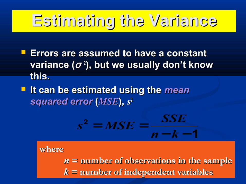
Errors are assumed to have a constant Errors are assumed to have a constant variance (variance (σσ 22), but we usually don’t know ), but we usually don’t know this.this.

It can be estimated using the It can be estimated using the mean mean squared errorsquared error ( (MSEMSE), ), ss2.2.

12

−−==

knSSE

MSEs

wherewherenn = number of observations in the sample = number of observations in the samplekk = number of independent variables = number of independent variables

4-34

Estimating the VarianceEstimating the Variance

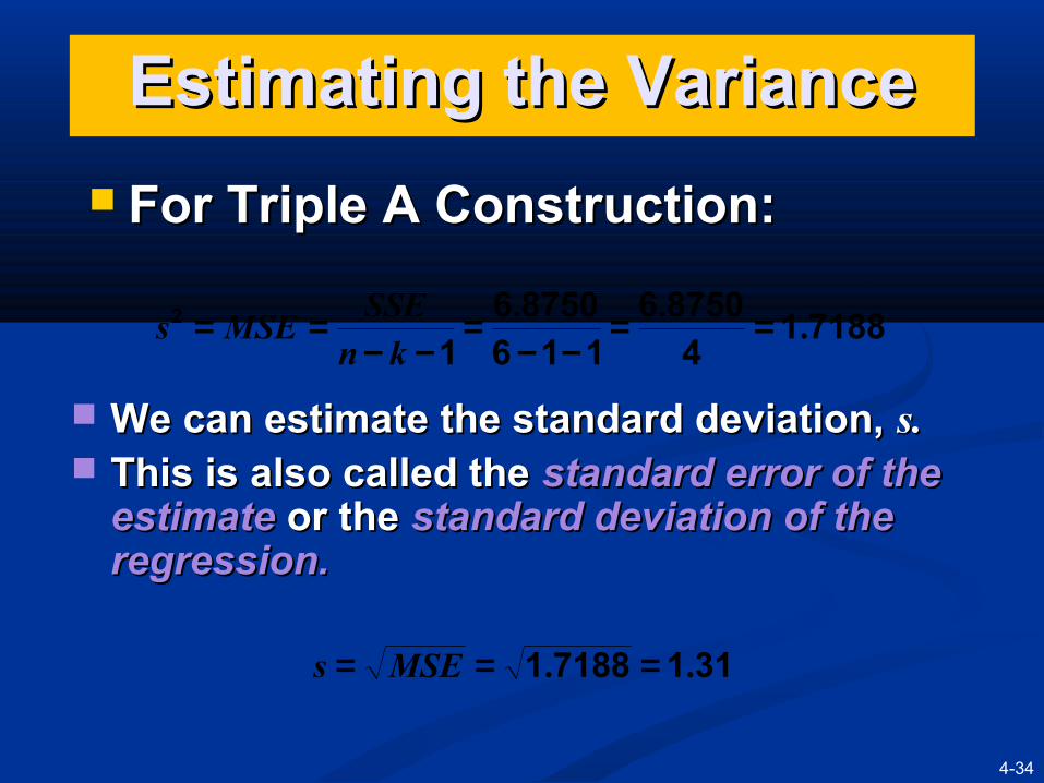
For Triple A Construction:For Triple A Construction:

718814

87506116

875061

2 ... ==

−−=

−−==

knSSE

MSEs

We can estimate the standard deviation, We can estimate the standard deviation, s.s. This is also called the This is also called the standard error of the standard error of the

estimateestimate or the or the standard deviation of the standard deviation of the regression.regression.

31171881 .. === MSEs

4-35

Testing the Model for Testing the Model for SignificanceSignificance

When the sample size is too small, you When the sample size is too small, you can get good values for can get good values for MSEMSE and and rr22 even if there is no relationship between even if there is no relationship between the variables.the variables.

Testing the model for significance Testing the model for significance helps determine if the values are helps determine if the values are meaningful.meaningful.

We do this by performing a statistical We do this by performing a statistical hypothesis test.hypothesis test.

Testing the Model for SignificanceTesting the Model for Significance

We start with the general linear We start with the general linear modelmodel

εββ ++= XY 10

If If ββ 11 = 0, the null hypothesis is that there is = 0, the null hypothesis is that there is nono relationship between relationship between XX and and Y.Y.

The alternate hypothesis is that there The alternate hypothesis is that there isis a a linear relationship (linear relationship (ββ 11 ≠ 0).≠ 0).

If the null hypothesis can be rejected, we If the null hypothesis can be rejected, we have proven there is a relationship.have proven there is a relationship.

We use the We use the FF statistic for this test. statistic for this test.

4-37

Testing the Model for Testing the Model for SignificanceSignificance

The The FF statistic is based on the statistic is based on the MSEMSE and and MSR:MSR:

kSSR

MSR =

wherewherekk = = number of independent variables in the modelnumber of independent variables in the model

The The FF statistic is: statistic is:

MSEMSR

F = This describes an This describes an FF distribution with: distribution with:

degrees of freedom for the numerator = degrees of freedom for the numerator = dfdf11 = = kk

degrees of freedom for the denominator = degrees of freedom for the denominator = dfdf22 = = nn – – kk – 1 – 1

4-38

Testing the Model for SignificanceTesting the Model for Significance

If there is very little error, the If there is very little error, the MSEMSE would be would be small and the small and the FF--statistic would be large statistic would be large indicating the model is useful.indicating the model is useful.

If the If the FF-statistic is large-statistic is large, the significance , the significance level (level (pp-value) will be low, indicating it is -value) will be low, indicating it is unlikely this would have occurred by unlikely this would have occurred by chance.chance.

So when the So when the FF--value is large, value is large, we can reject we can reject the null hypothesisthe null hypothesis and accept that there is a and accept that there is a linear relationship between linear relationship between XX and and YY and the and the values of the values of the MSEMSE and and rr22 are meaningful. are meaningful.

Steps in a Hypothesis TestSteps in a Hypothesis Test

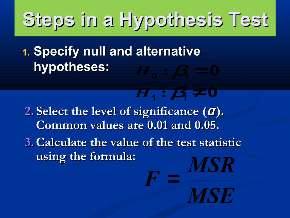
1.1. Specify null and alternative Specify null and alternative hypotheses:hypotheses: 010 =β:H

011 ≠β:H2.2. Select the level of significance (Select the level of significance (αα ). ).

Common values are 0.01 and 0.05.Common values are 0.01 and 0.05.3.3. Calculate the value of the test statistic Calculate the value of the test statistic

using the formula:using the formula:

MSEMSR

F =

Steps in a Hypothesis TestSteps in a Hypothesis Test4.4. Make a decision using one of the Make a decision using one of the

following methods:following methods:a)a) Reject the null hypothesis if the test statistic is greater than Reject the null hypothesis if the test statistic is greater than

the the FF-value from the table in Appendix D. Otherwise, do not -value from the table in Appendix D. Otherwise, do not reject the null hypothesis:reject the null hypothesis:

21 ifReject dfdfcalculated FF ,,α>

kdf =1

12 −−= kndf

b)b) Reject the null hypothesis if the observed significance Reject the null hypothesis if the observed significance level, or level, or pp-value, is less than the level of significance -value, is less than the level of significance ((αα ). Otherwise, do not reject the null hypothesis:). Otherwise, do not reject the null hypothesis:

)( statistictest calculatedvalue- >= FPp

α<value- ifReject p


Step 1.Step 1.HH00: : ββ 11 = 0 = 0 (no linear relationship (no linear relationship between between XX and and YY))HH11: : ββ 11 ≠ 0 ≠ 0 (linear relationship exists (linear relationship exists between between XX and and YY))Step 2.Step 2.

Select Select αα = 0.05 = 0.05

6250151625015

.. ===

kSSR

MSR

09971881625015

... ===

MSEMSR

F

Step 3.Step 3.Calculate the value of the test statistic.


Step 4.Step 4.Reject the null hypothesis if the test statistic is greater than the F-value in Appendix D.

dfdf11 = = kk = 1 = 1

dfdf22 = = nn – – kk – 1 = 6 – 1 – 1 = 4 – 1 = 6 – 1 – 1 = 4

The value of The value of FF associated with a 5% level of associated with a 5% level of significance and with degrees of freedom 1 and 4 is significance and with degrees of freedom 1 and 4 is found in Appendix D.found in Appendix D.

FF0.05,1,40.05,1,4 = 7.71 = 7.71

FFcalculatedcalculated = 9.09 = 9.09

Reject Reject HH00 because 9.09 > 7.71 because 9.09 > 7.71

F = 7.71

0.05

9.09


Figure 4.5

We can conclude there is a We can conclude there is a statistically significant statistically significant relationship relationship between between XX and and Y.Y.

The The rr22 value of 0.69 means about value of 0.69 means about 69% of the variability in sales (69% of the variability in sales (YY) ) is explained by local payroll (is explained by local payroll (XX).).

4-44

Analysis of Variance Analysis of Variance (ANOVA) Table(ANOVA) Table

When software is used to develop a regression When software is used to develop a regression model, an model, an ANOVA table ANOVA table is typically created that is typically created that shows the observed significance level (shows the observed significance level (pp-value) for -value) for the calculated the calculated FF value. value.

This can be compared to the level of significance This can be compared to the level of significance ((αα ) to make a decision.) to make a decision.

DFDF SSSS MSMS FF SIGNIFICANCESIGNIFICANCE

RegressionRegression kk SSRSSR MSRMSR = = SSRSSR//kk MSRMSR//MSEMSE PP((FF > > MSRMSR//MSEMSE))

ResidualResidual nn - - kk - 1 - 1 SSESSE MSEMSE = = SSESSE//((nn - - kk - 1) - 1)

TotalTotal nn - 1 - 1 SSTSST

Table 4.4

4-45

ANOVA for Triple A ConstructionANOVA for Triple A Construction

Because this probability is less than 0.05, we reject Because this probability is less than 0.05, we reject the null hypothesis of no linear relationship and the null hypothesis of no linear relationship and conclude there is a linear relationship between conclude there is a linear relationship between XX and and Y.Y.

Program 4.1C (partial)

PP((FF > 9.0909) = 0.0394 > 9.0909) = 0.0394

4-46

Multiple Regression AnalysisMultiple Regression Analysis Multiple regression models are extensions

to the simple linear model and allow the creation of models with more than one independent variable.

YY = = ββ 00 + + ββ 11XX11 + + ββ 22XX22 + … + + … + ββ kkXXkk + + εεwherewhere

YY = = dependent variable (response variable)dependent variable (response variable)XXii = = iithth independent variable (predictor or explanatory independent variable (predictor or explanatory variable)variable)ββ 00 = = intercept (value of intercept (value of YY when all when all XXii = 0)= 0)

ββ ii = = coefficient of the coefficient of the iithth independent variable independent variable

kk = = number of independent variablesnumber of independent variablesεε == random errorrandom error

Multiple Regression AnalysisMultiple Regression Analysis

To estimate these values, a sample is To estimate these values, a sample is taken the following equation developedtaken the following equation developed

kk XbXbXbbY ++++= ...ˆ22110

wherewhere == predicted value of predicted value of YYbb00 = = sample intercept (and is an estimate of sample intercept (and is an estimate of ββ 00))

bbii == sample coefficient of the sample coefficient of the iithth variable (and variable (and is an estimate of is an estimate of ββ ii))

Y

4-48

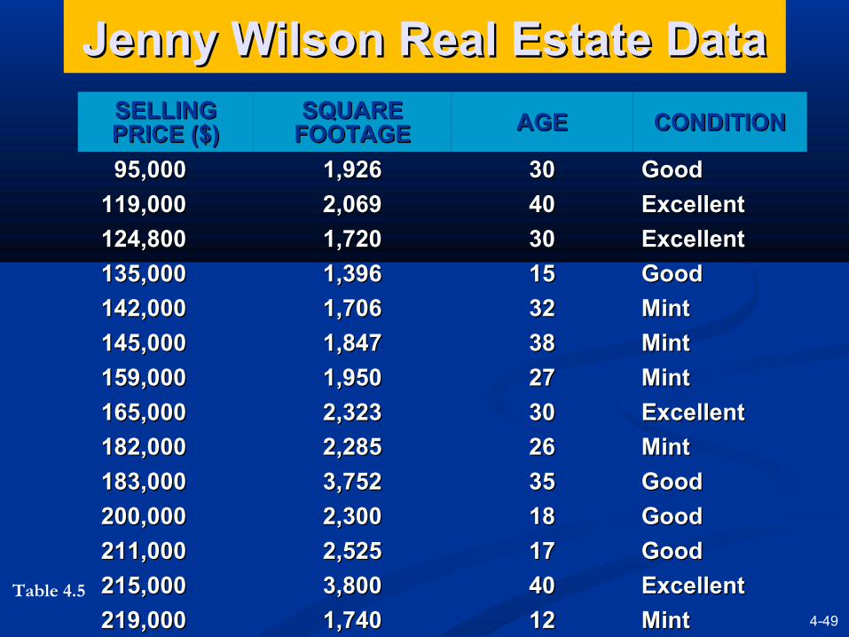
Jenny Wilson RealtyJenny Wilson RealtyJenny Wilson wants to develop a model to Jenny Wilson wants to develop a model to determine the suggested listing price for determine the suggested listing price for houses based on the size and age of the houses based on the size and age of the house.house.

22110ˆ XbXbbY ++=

wherewhere == predicted value of dependent variable predicted value of dependent variable (selling price)(selling price)bb00 = = YY intercept intercept

XX11 and and XX22 = = value of the two independent value of the two independent variables (square footage and age) respectivelyvariables (square footage and age) respectivelybb1 1 andand bb22 = =slopes for slopes for XX11 and and XX22 respectively respectively

Y

She selects a sample of houses that have sold She selects a sample of houses that have sold recently and records the data shown in Table 4.5recently and records the data shown in Table 4.5

4-49

Jenny Wilson Real Estate DataJenny Wilson Real Estate DataSELLING SELLING PRICE ($)PRICE ($)

SQUARE SQUARE FOOTAGEFOOTAGE AGEAGE CONDITIONCONDITION

95,00095,000 1,9261,926 3030 GoodGood

119,000119,000 2,0692,069 4040 ExcellentExcellent


135,000135,000 1,3961,396 1515 GoodGood

142,000142,000 1,7061,706 3232 MintMint

145,000145,000 1,8471,847 3838 MintMint

159,000159,000 1,9501,950 2727 MintMint


182,000182,000 2,2852,285 2626 MintMint

183,000183,000 3,7523,752 3535 GoodGood

200,000200,000 2,3002,300 1818 GoodGood

211,000211,000 2,5252,525 1717 GoodGood


219,000219,000 1,7401,740 1212 MintMintTable 4.5

4-50

Jenny Wilson RealtyJenny Wilson Realty

Program 4.2A

Input Screen for the Jenny Wilson Input Screen for the Jenny Wilson Realty Multiple Regression ExampleRealty Multiple Regression Example

4-51


Program 4.2B

Output for the Jenny Wilson Realty Multiple Output for the Jenny Wilson Realty Multiple Regression ExampleRegression Example

Evaluating Multiple Evaluating Multiple Regression ModelsRegression Models

Evaluation is similar to simple linear Evaluation is similar to simple linear regression models.regression models. The The pp-value for the -value for the FF-test and -test and rr22 are are

interpreted the same.interpreted the same. The hypothesis is different because there is The hypothesis is different because there is

more than one independent variable.more than one independent variable. The The FF-test is investigating whether all -test is investigating whether all

the coefficients are equal to 0 at the same the coefficients are equal to 0 at the same time.time.

Evaluating Multiple Evaluating Multiple Regression ModelsRegression Models

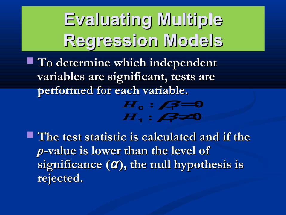
To determine which independent To determine which independent variables are significant, tests are variables are significant, tests are performed for each variable.performed for each variable.

010 =β:H011 ≠β:H

The test statistic is calculated and if the The test statistic is calculated and if the pp-value is lower than the level of -value is lower than the level of significance (significance (αα ), the null hypothesis is ), the null hypothesis is rejected.rejected.

4-54

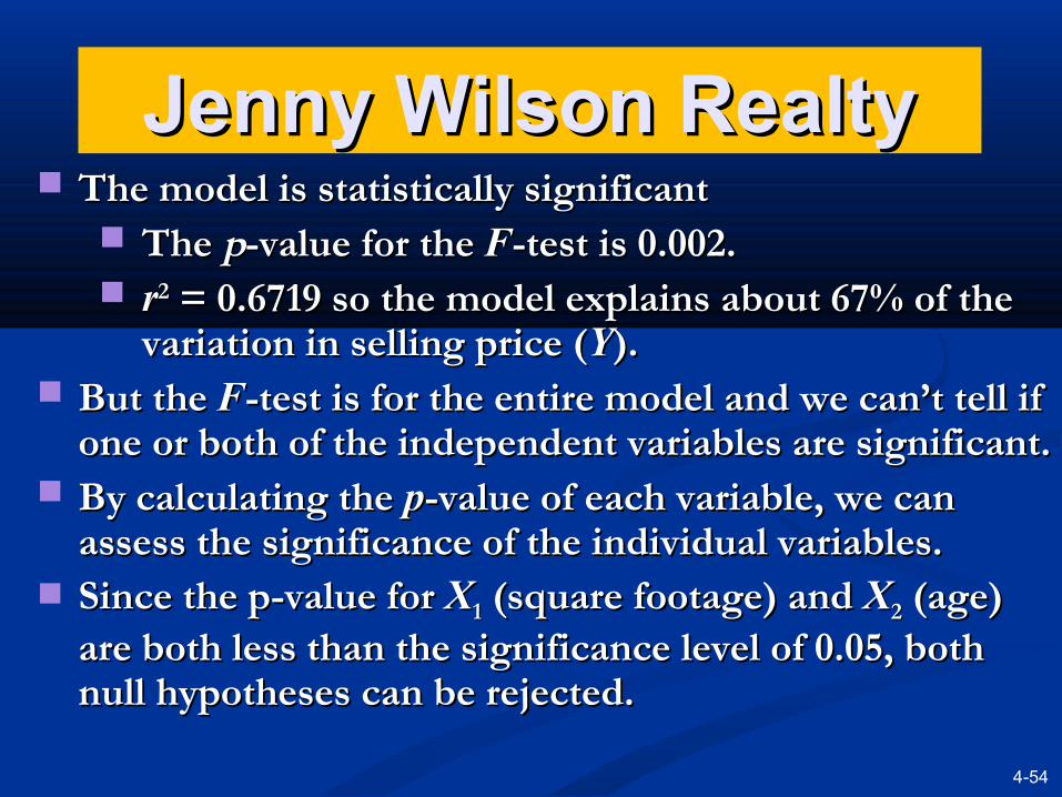
Jenny Wilson RealtyJenny Wilson Realty The model is statistically significantThe model is statistically significant

The The pp-value for the -value for the FF-test is 0.002.-test is 0.002. rr22 = 0.6719 so the model explains about 67% of the = 0.6719 so the model explains about 67% of the

variation in selling price (variation in selling price (YY).). But the But the FF-test is for the entire model and we can’t tell if -test is for the entire model and we can’t tell if

one or both of the independent variables are significant.one or both of the independent variables are significant. By calculating the By calculating the pp-value of each variable, we can -value of each variable, we can

assess the significance of the individual variables.assess the significance of the individual variables. Since the p-value for Since the p-value for XX11 (square footage) and (square footage) and X X22 (age) (age)

are both less than the significance level of 0.05, both are both less than the significance level of 0.05, both null hypotheses can be rejected.null hypotheses can be rejected.

Binary or Dummy VariablesBinary or Dummy Variables BinaryBinary (or (or dummydummy or or indicatorindicator) )

variables are special variables variables are special variables created for qualitative data.created for qualitative data.

A dummy variable is assigned a A dummy variable is assigned a value of 1 if a particular condition value of 1 if a particular condition is met and a value of 0 otherwise.is met and a value of 0 otherwise.

The number of dummy variables The number of dummy variables must equal one less than the must equal one less than the number of categories of the number of categories of the qualitative variable.qualitative variable.

4-56

Jenny Wilson RealtyJenny Wilson Realty Jenny believes a better model can be Jenny believes a better model can be

developed if she includes information developed if she includes information about the condition of the property.about the condition of the property.

XX33 = 1 if house is in excellent condition= 1 if house is in excellent condition

= 0 otherwise= 0 otherwiseXX44 = 1 if house is in mint condition= 1 if house is in mint condition

= 0 otherwise= 0 otherwise Two dummy variables are used to describe the Two dummy variables are used to describe the

three categories of condition.three categories of condition. No variable is needed for “good” condition No variable is needed for “good” condition

since if both since if both XX33 and and XX44 = 0, the house must be in = 0, the house must be in good condition.good condition.

4-57


Program 4.3A

Input Screen for the Jenny Wilson Realty Input Screen for the Jenny Wilson Realty Example with Dummy VariablesExample with Dummy Variables

4-58


Program 4.3B

Output for the Jenny Wilson Realty Example Output for the Jenny Wilson Realty Example with Dummy Variableswith Dummy Variables

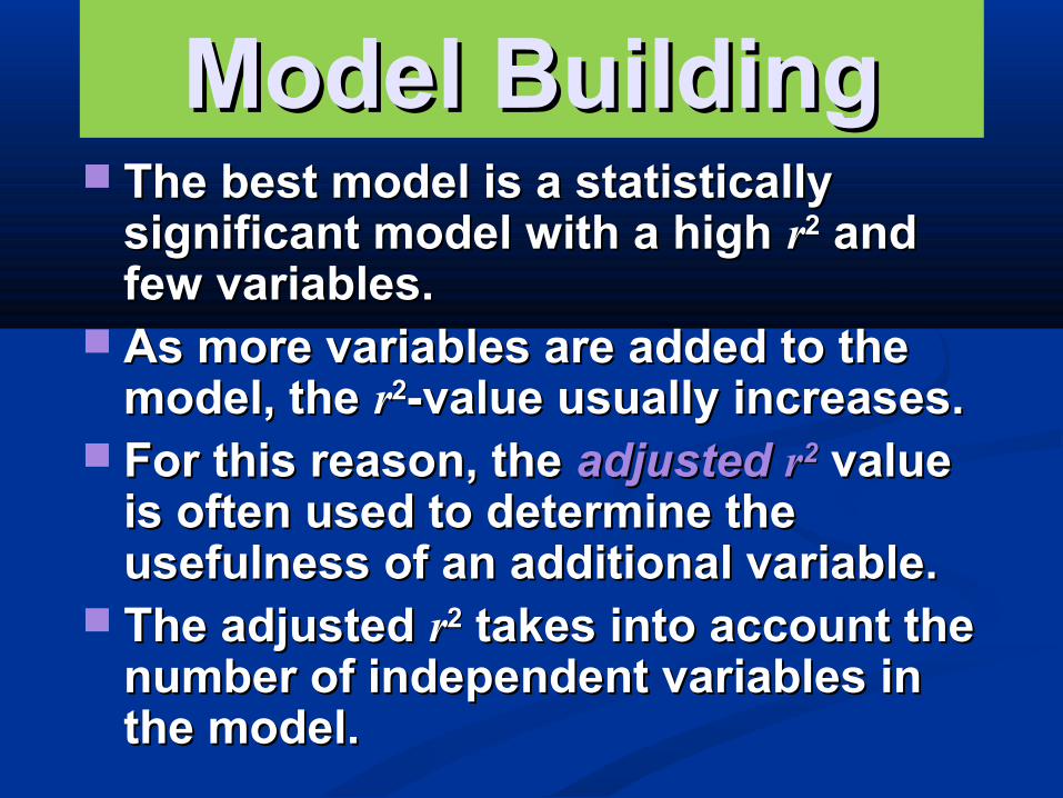
Model BuildingModel Building The best model is a statistically The best model is a statistically

significant model with a high significant model with a high rr22 and and few variables.few variables.

As more variables are added to the As more variables are added to the model, the model, the rr22-value usually increases.-value usually increases.

For this reason, the For this reason, the adjusted adjusted rr22 value value is often used to determine the is often used to determine the usefulness of an additional variable.usefulness of an additional variable.

The adjusted The adjusted rr22 takes into account the takes into account the number of independent variables in number of independent variables in the model.the model.

Model BuildingModel Building

SSTSSE

SSTSSR −== 12r

The formula for The formula for rr22

The formula for adjusted The formula for adjusted rr22

)/(SST)/(SSE

11

1 Adjusted 2

−−−−=

nkn

r

As the number of variables increases, the As the number of variables increases, the adjusted adjusted rr22 gets smaller unless the increase gets smaller unless the increase due to the new variable is large enough to due to the new variable is large enough to offset the change in offset the change in k.k.

Model BuildingModel Building In general, if a new variable increases the In general, if a new variable increases the

adjusted adjusted rr22, it should probably be included in the , it should probably be included in the model.model.

In some cases, variables contain duplicate In some cases, variables contain duplicate information.information.

When two independent variables are correlated, When two independent variables are correlated, they are said to be they are said to be collinear.collinear.

When more than two independent variables are When more than two independent variables are correlated, correlated, multicollinearitymulticollinearity exists. exists.

When multicollinearity is present, When multicollinearity is present, hypothesis hypothesis tests for the individual coefficients are not valid tests for the individual coefficients are not valid but the model may still be useful.but the model may still be useful.

4-62

Nonlinear RegressionNonlinear Regression In some situations, variables are not In some situations, variables are not

linear.linear. Transformations may be used to turn Transformations may be used to turn

a nonlinear model into a linear model.a nonlinear model into a linear model.

** **

** ** *

Linear relationshipLinear relationship Nonlinear relationshipNonlinear relationship

**** **

****

*

4-63

Colonel MotorsColonel Motors Engineers at Colonel Motors want to use

regression analysis to improve fuel efficiency. They have been asked to study the impact of

weight on miles per gallon (MPG).

MPGMPG

WEIGHT WEIGHT (1,000 (1,000 LBS.)LBS.) MPGMPG

WEIGHT WEIGHT (1,000 (1,000 LBS.)LBS.)

1212 4.584.58 2020 3.183.18

1313 4.664.66 2323 2.682.68

1515 4.024.02 2424 2.652.65

1818 2.532.53 3333 1.701.70

1919 3.093.09 3636 1.951.95

1919 3.113.11 4242 1.921.92

Table 4.6

4-64

Colonel MotorsColonel Motors

Figure 4.6A

Linear Model for MPG DataLinear Model for MPG Data

4-65


Program 4.4

This is a useful model with a small This is a useful model with a small FF-test -test for significance and a good for significance and a good rr22 value. value.

Excel Output for Linear Regression Excel Output for Linear Regression Model with MPG DataModel with MPG Data

4-66


Figure 4.6B

Nonlinear Model for MPG DataNonlinear Model for MPG Data

4-67


The nonlinear model is a quadratic model.The nonlinear model is a quadratic model. The easiest way to work with this model is The easiest way to work with this model is

to develop a new variable.to develop a new variable.2

2 weight)(=X This gives us a model that can be This gives us a model that can be

solved with linear regression software:solved with linear regression software:

22110 XbXbbY ++=ˆ

4-68


Program 4.5

A better model with a smaller A better model with a smaller FF-test for -test for significance and a larger adjusted significance and a larger adjusted rr22 value value

21 43230879 XXY ...ˆ +−=

Cautions and PitfallsCautions and Pitfalls If the assumptions are not met, the If the assumptions are not met, the

statistical test may not be valid.statistical test may not be valid. Correlation does not necessarily mean Correlation does not necessarily mean

causation.causation. Multicollinearity makes interpreting Multicollinearity makes interpreting

coefficients problematic, but the model may coefficients problematic, but the model may still be good.still be good.

Using a regression model beyond the range Using a regression model beyond the range of of XX is questionable, as the relationship may is questionable, as the relationship may not hold outside the sample data.not hold outside the sample data.

Cautions and PitfallsCautions and Pitfalls AA t t-test for the intercept (-test for the intercept (bb00) may be ignored ) may be ignored

as this point is often outside the range of as this point is often outside the range of the model.the model.

A linear relationship may not be the best A linear relationship may not be the best relationship, even if the relationship, even if the FF-test returns an -test returns an acceptable value.acceptable value.

A nonlinear relationship can exist even if a A nonlinear relationship can exist even if a linear relationship does not.linear relationship does not.

Even though a relationship is statistically Even though a relationship is statistically significant it may not have any practical significant it may not have any practical value.value.

TutorialTutorial

Lab Practical : Spreadsheet Lab Practical : Spreadsheet

1 - 71

Further ReadingFurther Reading

Render, B., Stair Jr.,R.M. & Hanna, M.E. (2013) Quantitative Analysis for Management, Pearson, 11th Edition

Waters, Donald (2007) Quantitative Methods for Business, Prentice Hall, 4 th Edition.

Anderson D, Sweeney D, & Williams T. (2006) Quantitative Methods For Business Thompson Higher Education, 10th Ed.

QUESTIONS?QUESTIONS?

tbs910 regression models

Business

nonlinear regression

regression model4

regression analysis5

multiple regression

use of regression analysis

multiple regression

regression line e

response variable