technical and economic considerations of … · simulation of the amine absorption post-combustion...

International Journal of Advances in Engineering & Technology, Nov., 2014.

©IJAET ISSN: 22311963

1549 Vol. 7, Issue 5, pp. 1549-1581

TECHNICAL AND ECONOMIC CONSIDERATIONS OF POST -

COMBUSTION CARBON CAPTURE IN A COAL FIRED POWER

PLANT

Mohammed Isah Yakub1*, Mohamed, Samah2 and Sule Umar Danladi3 1Department of Chemical Engineering,

Abubakar Tafawa Balewa University P.M.B 0248 Bauchi Nigeria 2Department of Chemical Engineering, the University of Khartoum, Sudan

3Department of Chemical Engineering, the Federal Polytechnic P.M.B 55 Bida, Nigeria

ABSTRACT Techno-economic consideration of post combustion carbon capture in a coal fired power plant (500MW) was

carried out. Primary (MEA), secondary (DEA) and tertiary (MDEA) amines were analysed regarding their

tendency to corrode the equipments and their performance in the absorption and stripping columns using Aspen

Hysys® 7.2 software. From the simulation work, DEA showed better performance. The DEA process was

optimised to find the optimum parameters that explore the trade-off between efficiency and operating and

capital costs at an acceptable operating point. The cost of commissioning and operating the capture plant was

also estimated and different cost metrics were calculated for the plant feasibility. The levelized cost of electricity

increased by £0.028/kWh compared to the original cost of £0.105/kWh. The cost of CO2 treatment was found to

be £26.8/ton which is higher compared to UK carbon floor price (2012) of £16/ton CO2. Finally, the decision

will be either to operate the power plant without a capture plant and pay the carbon tax or retrofitting the

power plant for carbon capture and pay the cost of treating the CO2. However, if the emphasis is on

environmental consideration, the retrofitting becomes the best option.

KEYWORDS: Modelling; simulation; amine; post-combustion; carbon capture, Hysys® 7.2

I. INTRODUCTION

Greenhouse gas emissions are serious dilemma that concerns the scientist and politician together,

which accelerate the pace of finding solutions. As such, different regulation are issued a year after a

year forcing polluters to cut these emissions. Several methods are currently being investigated

towards reducing carbon emissions among which include higher efficiency energy conversion

processes, fuel switching and of particular interest, carbon capture and storage, CCS [1]. In the higher

efficiency conversion process, carbon reduction is performed prior to the combustion. This operate

based upon the increased energy output of power generation plants for every unit of fuel used through

more efficient processes which in turn reduces the mass of carbon dioxide released into the

atmosphere per unit of energy produced. An example of a higher efficiency conversion process is

integrated gasification combined cycles (IGCC) which can be modelled as heat engines [2, 3, 4]. By

combining two heat engines cycles, the overall efficiency will increase. However, to implement such

processes, it may require installing additional and retrofitting new equipment onto the existing power

plant which will result in accrued capital costs. Another solution to increased efficiency with or

without combined cycles is to increase the temperature differential between the heat input and the



1550 Vol. 7, Issue 5, pp. 1549-1581

rejected heat by increasing the temperature and pressure of the cycle but there may not be many

materials that can withstand such high levels of the temperature and pressure [2, 3, 4].

Fuel switching is another option for reduction of CO2 emissions into the atmosphere. The objective of

fuel switching is to utilize means that possess lower carbon content in its composition or produces less

emission in its energy generation [3, 5]. In doing so, combusting these fuel sources or its generation

methods will result in lower CO2 emissions into the atmosphere. Renewable sources of energy such

as solar, wind, wave, etc are examples of fuel switching options as they do not emit CO2 during the

generation. However, despite this simple and straightforward as well as advantageous solution to

carbon dioxide emissions, the energy output of these fuels is lower and larger amounts of the fuel

sources are required compared to fossil sources. This may result in higher capital and operating costs

[3, 5]. Biomass co-firing is one of the options currently used in the industry. It is a process where a

proportion of a biomass fuel source is burnt together with a proportion of coal. The energy density of

coal is significantly greater than biomass and therefore energy output will be lower. Natural gas is

also another alternative fuel as its combustion emits lower levels of harmful substances into the

atmosphere. Availability of these alternative fuel sources in the long run may also be an issue [3, 5].

CCS has been considered as an option for limiting CO2 emissions from the combustion of fossil fuels

[1]. This approach includes pre-combustion capture, post-combustion capture and oxy-fuel

combustion [2, 3, 4, 5]. In pre-combustion capture, the carbon is removed prior to the combustion

process through a series of chemical reactions or processes and it may include the methods of higher

energy conversion processes and fuel switching. In post combustion capture, the removal of CO2 is

done after the combustion of the fuel source. In oxy-fuel capture, the fuel source is combusted with

O2/air and the flue gas is cleaned for a carbon free stream [6, 7]. The post-combustion capture

technology is more feasible as opposed to the other carbon capture approaches because of its lower

cost and retrofitting option. It allows implementation without incurring relatively larger capital and

operating costs and allows more plant flexibility as well [7].

Generally, carbon capture plants is still under the development stages, thus great efforts are focused

on the most favourable capture method to establish optimum conditions. Hysys® software is used

extensively in this direction. Many attempts recently to simulate the carbon capture plant, especially

amine based, are carried out for the purposes of feasibility study and the design aiding. Simulation of

the amine absorption post-combustion technology is considered as a complex matter, as accurate

rigorous models are required [8]. Most modelling focuses mainly on parameter optimization such as

the flue gas flow rate and its effect, CO2 concentration, solvent temperature and pressure, recycle

stream, heat and work duties along with other parameters as reported by Singh et al. (2003) [9]; Fisher

et al. (2005) [10]. An attempt to analyse a 500MW existing coal power plant with monoethanolamine

(MEA) for CO2 capture in Canada was carried out by Ali (2004) [11] using ASPEN PLUS. The

pressure profile for the columns was of utmost priority to analyse the hydrodynamic performance for

design purposes. Further development for the same case was done by Alie et al. (2005) [12] to

improve the convergence in ASPEN.

Another trial was performed for 600MW bituminous coal fired power plant, using MEA in ASPEN

software for column design. The optimized parameter was the thermal energy consumption. 3.0

GJ/ton was found as the minimum achieved by 40 wt% MEA solutions for 13 %v/v CO2 in flue gas

and 90% recovery [13]. A similar attempt was done by Oi, (2007) [14]. The work of Khakdaman et al.

(2008) [15] focused on improving efficiency, using a mixture of solvents, diethanolamine (DEA) and

N-methyldiethanolamine (MDEA) for a fixed CO2 recovery and heat duty in columns. The simulation

proved that a better capacity could be achieved when solvent blends are used.

In this present study, initial attempts were made at simulating a carbon capture and storage system

using a chemical absorption process with chilled ammonia as the solvent. Our investigations revealed

that the chilled ammonia process has many advantages over the conventional amine solvents in terms

of cost efficiency and technical viability. One example of these advantages is the lower heat of

absorption which leaves the process in less need of heating requirements. This is also in accordance

with Darde et al (2010) [16]. However, the process met a lot of difficulties due to the absence of

suitable property packages in Aspen HYSYS and lack of data (such as interaction parameters to use

other conventional fluid packages) and therefore decided to continue with the amine solvents.



1551 Vol. 7, Issue 5, pp. 1549-1581

The objective of this study was to carry out a technical and economic analysis of carbon capture in

500MW full capacity (420MW generation) coal fired power plant using Hysys® simulation to

achieve a above 90% recovery of CO2 with a purity of 99% using amine solvents.

This article is structured in to different sections: Methodology, results and discussions, conclusion,

future work, acknowledgment, references and appendix.

II. METHODOLOGY

2.1 Feed Composition The plant feed comprises of mainly carbon dioxide, nitrogen, water and oxygen which is obtained

from a 500 MW plant. Table 1 below gives a typical composition of the flue gas from a coal fired

power plant. The operational window of the power plant is assumed to be 8000 hours annually. The

desired removal of carbon dioxide from the inlet stream is to be approximately 90% of the original in-

flow in to the absorption column.

2.2 Process Description The absorber column is operating at certain pressure with a pressure drop across each stage. The

absorber column consists of packings which maximise gas/liquid contact and give sufficient liquid

hold-up for reaction between CO2 and amine solvent to take place. The flue gas leaves the top of the

absorber column with a largely reduced concentration of CO2 at a particular temperature and

pressure. The gas leaving the top of the absorber is released into the atmosphere with a significantly

reduced concentration of CO2. The solvent, now rich with CO2 leaves the bottom of the absorber

column at a specific temperature and pressure. The bottom stream is then pumped to increase the

pressure before entering the 2 way heat exchanger. The 2 way heat exchanger brings into contact the

rich-in-CO2 bottom stream from the absorber column and the lean CO2 solvent which exits the

bottom of the stripper column. The CO2 rich stream is heated before it enters the stripping unit where

CO2 is stripped off from the amine solvent. The lean solvent is then cooled and reused in the

absorption column. A schematic process flow diagram is shown in Figure 1 below.

Table 1: Coal Fired Power Plant Flue Gas [3]

Capacity (MW) 500

Temperature (°C) 50

Pressure (Kpa) 110

Molar Flow (Kmole/h) 71280

Volume Flow (m3/h) 1914000

Composition (mole percent)

Carbon Dioxide (CO2) 15.00

Nitrogen (N2) 77.00

Sulphur Dioxide (SO2) 0.00001

Nitrogen Oxides (NOx) 0.00005

Water (H2O) 5.00

Carbon Monoxide (CO) 0.00001

Oxygen (O2) 3.00



1552 Vol. 7, Issue 5, pp. 1549-1581

Figure 1: Schematic of amine scrubbing process in CO2 post-combustion capture

III. RESULTS AND DISCUSSIONS

3.1 Amine Selection

Amine selection for carbon capture is based on three important factors: Corrosiveness, absorption

capacity and stripping condition. A study of the absorption and desorption (stripping) capacity of the

amines is also necessary to avoid the need for extremely tall towers that can offer the process enough

area and residence time for the CO2 transfer from/towards the solvent. It is well known that corrosion

effect of amines varies depending on the class and concentration used. No tertiary amine

concentration can have corrosion rates similar to those of primary and secondary amines, so a

concentration of 50%w/w as suggested by the literature [17] was used to compare the behaviour of

MDEA against MEA and DEA. Similarly, 30%w/w of the secondary amine DEA, and 16.5%w/w

MEA (primary amine) were employed. The results of simulations are shown in Figures (2 to 4) for the

three different amines.

50

56

62

68

74

93

94

95

96

97

98

99

100

101

10 15 20 25 30 35

Refl

ux R

ati

o (

R=

L/

D)

CO

2C

ap

tured

(%

)

Number of Stages

Absorption/Stripping Performance

MEA - Coal Fired Plant

1 bar 5 bar 10 bar Stripping

Figure 2: MEA performance for a Coal Fired Power Plant

Figure 2: MEA performance for a Coal Fired Power Plant



1553 Vol. 7, Issue 5, pp. 1549-1581

From the Figure 3, it is seen that a primary amine, MEA is very appropriate for absorb CO2 in the

flue gas with capture over 90% as required (Audit report, 2009). However, from the stripping curve

read from the right side of the plot, it is also observed that the system requires huge reflux ratios in

separation which suggests that this process is not cost effective.

Figure 3: DEA performance for a Coal Fired Power Plant

Performance of absorber and stripper in a carbon capture plants at different pressures, for DEA based

solvent showed reduction in affinity with the acid gas, requiring further efforts in absorption. The

process requires either high pressures or more than 23 stages in absorption for an atmospheric

pressure absorber to captures over 90% CO2. On the other hand, stripping has been improved to very

acceptable levels, with reflux ratios within the range 2– 3.2 as shown in the Figure 3.

Tertiary amines as MDEA are very well known to have limited affinity for acid gases in comparison

to primary and secondary amines as earlier stated. This fact can easily be observed in Figures 4 above

where no operating pressure can achieve the target capture, making of this option the least favourable

in terms of absorption rate. Nevertheless, the stripping process is much easier with very low reflux

ratio in relatively small columns.

Figure 4: MDEA performance for a Coal Fired Power Plant

It is now clear that using only tertiary amines to capture acid gases is not technically feasible due to

the high number of stages needed for absorption at the required level, no matter how easy the

2.5

2.6

2.7

2.8

2.9

3.0

3.1

3.2

3.3

75

80

85

90

95

100

10 15 20 25 30 35

Refl

ux R

ati

o (

R=

L/

D)

CO

2C

ap

tured

(%

)

Number of Stages


DEA - Coal Fired Plant


2.0

2.1

2.2

2.3

2.4

2.5

2.6

2.7

2.8

2.9

3.0

20

25

30

35

40

45

50

55

60

65

70

10 15 20 25 30 35

Refl

ux R

ati

o (

R=

L/

D)

CO

2C

ap

tured

(%

)

Number of Stages


MDEA - Coal Fired Plant




1554 Vol. 7, Issue 5, pp. 1549-1581

stripping process could be. On the other hand, primary amines showed a good tendency to removing

CO2 from the flue gas with the additional constraint of difficult separation in the recovery process.

This would be an advisable option only in case of diluted flue gas stream. The secondary amine DEA

showed the best performance in terms of affinity for the acid gas and separation viability with

moderate reflux ratio making it suitable for the design considered in this study.

3.2 Process Modelling and Simulation

From the process flow diagram in the Figure 5 below, it is necessary to ensure that the inlet stream

can overcome the head loss through the absorption towers. It is also well known that a higher

operating pressure in tower will increase the CO2 absorption into the liquid phase, however, this

process is very expensive due to the high energy requirement to increase the pressure of the large flue

gas flow rate coming from the power station and therefore lower pressures are preferred despite their

lower performance within the absorption equipment, thus, only the necessary head was supplied to the

flue gas using blower to travel across the absorption stages. A 2 kPa pressure drop was assumed for

each stage in the absorption towers.

Amine absorption processes for CO2 capture are typically carried out with aqueous amine solutions

with concentrations between 25-30% by mass, which enters at 45°C on the top of the absorber while

the acid gas enters in the tower at the bottom and leaves the equipment at the top as a sweet gas with

very low CO2 concentration (under 1.5% mole fraction). This equipment was designed by modifying

the number of stages, until the absorption rose over 90%. It is necessary to clarify that temperatures

over 125 ºC can cause amine degradation and therefore there is a software limitation associated with

the fluid package available for this purpose (Amines Package in Aspen HYSYS), warnings about the

accuracy of calculation for the properties of streams above 125 °C are shown during the simulation,

this operating condition was established to reach a desired recovery and top composition of CO2 and

the solver was run until convergence was reached. A bottom pressure of 215 kPa and a condenser

temperature of 40 ºC achieved up to 91% recovery of CO2 with an initial 3.81 reflux ratio and CO2

purity on tops of 95.7% by mole. The bottom stream leaving the stripping column contains all the

amine used in absorbing the acid gas and was recycled. Enthalpy of the recycled stream was used to

preheat incoming feed to the tower as system heat integration.

The amine and water concentrations in the treated gas stream were very low and their accumulation

was observed when the recycle unit is connected. As the iterations reach convergence, the amine

required to keep the system stable is always under 1 kg/h, typically 0.5 kg/h. On the other hand, the

water balance shows that high temperatures in the recycled stream will increase the water loss in

absorption pushing for a high water make up, while low temperatures are difficult to reach due to the

high cooling demand in this stream. This balance deserves an economic analysis in order to establish

the equilibrium point in which the water consumption does not exceed the cooling expenses. Two

adjust units were used to vary different parameters in the process, one of them is used to change the

inlet gas flow based on the capacity of the power station and evaluate its impact on the capture

efficiency. The other was used to vary the inlet flow rate of amine to the absorber to ensure a good

CO2/mol Amine ratio for the absorption units.

The cooling requirements for this process are related to the heats that must be removed from the

condenser of the stripping column, where the amine is recovered, and an additional heat that must be

taken out in the recycled amine in to the absorber. This heat was taken out from the process by means

of heat exchangers. All the heat exchangers were designed to keep a temperature approach of 12.6 ºC.

The rate at which the makeup components are fed into the process could help reducing the effect of

the amine decomposition. In this case, purging some part of the used amine became necessary and a

greater make up was required in order to keep the chemical activity of the absorbent in the system.

As the flue gas coming from the power plant consist of low percentage of solids that could not be

simulated in Aspen HYSYS, a microfilter casing with special designed cartridges suitable for amines

operation was installed in the recycled amine stream coming from the bottom of the stripper, this

equipment is expected to retain solids captured from the flue gas during the absorption and

degradation products formed during the stripping procedure.

All pressure drops due to friction, tubing accessories and head losses were calculated and imposed on

hypothetical valves right after each pump in the process flow diagram. These valves will only account



1555 Vol. 7, Issue 5, pp. 1549-1581

for the energy required to move the streams through the pipes at the different levels of the plant and

do not include the pressure drops within the different pieces of equipment.

Figure 5: Process Flow Diagram



1556 Vol. 7, Issue 5, pp. 1549-1581

Table 2: Summary of material stream obtained from Hysys



1557 Vol. 7, Issue 5, pp. 1549-1581

Table 3: Summary of energy streams

3.3 Equipment Specification

Detail description of the procedure on how to determine all the parameters used in this section are

shown in the Appendix

3.3.1 Absorption column

Assumptions and design considerations:

CO2 absorption is carried out in a continuous counter current packed column, to achieve high

contact area between the flue gas and the solvent.

Both structured and random packing could be used, but random is chosen because it is

cheaper. Plastic Intalox® saddles are used to overcome the corrosive nature of Amines, beside

its high efficiency compared to ceramic [18].

DEA absorption has no tendency to produce foams in the absorption process [19].

Table 4: Absorption column specification

Column Details

Number of columns - 8

Number of stages - 301

Internals - Packed2

Internals Type - Intalox saddles (3_inche)2

HETP - 0.8468

Foaming Factor - 12

Maximum flooding % 843

Material of construction - Stainless steel

Column sizing

Section diameter m 61

Section height m 25.51

1 Obtained from the simulation 2 Assumed 3Calculated in appendix

3.3.2 Stripper column Assumptions and design considerations:

Solvent recovery is carried out in a stage wise distillation column.

Sieve plate is used among the different plate types, as it is cheap, has less tendency for fouling

and suitable for most applications [18].

DEA absorption has no tendency to produce foams in the absorption process [19].

Table 5: Stripper column specification

Column Details

Number of columns 8

Number of stages - 301

Internals - plate2

Internals Type - Sieve plate2

Tray spacing m 0.60962

Tray thickness mm 3.1752

Foaming Factor - 1



1558 Vol. 7, Issue 5, pp. 1549-1581

Maximum flooding % 653

Column sizing

Section diameter m 61

Section height m 181

1 Obtained from the simulation 2 Assumed 3 Calculated in appendix

3.3.3 Compressors

Table 6: Compressor specification

Specification Flue Gas Compression Compression to Storage

Operating Conditions

Qin m3/h 1’739,485 175,712

Qout m3/h 1’350,182 2,463

Pout bar 1.6 100

∆P bar 0.5 98.45

Pressure Ratio - 3:2 4:1

Inlet Temperature ºC 50 38.4

Polytropic Efficiency % 82.57

81.7

Compressor Details

Single/Multi stage - Single Stage Multi Stage

Intercooling? y/n No Yes

Material - Carbon Steel Carbon Steel

Type - Centrifugal fan / Axial blower Centrifugal Compressor

Compressor Disposition

Number of compressors - 5 9

Series - 0 3

Parallel - 5 3

3.3.4 Pumps and pipelines

Table 7: Pump specifications data

Specification Stripper Feed Make Up Recycle

Piping and Head Losses

Flow rate m3/h

16,390

0.079

16,223

Piping Inside Diameter in 21.6 0.1 32.3

∆P equipment kPa 20.0 0.0 450.2

∆P static kPa 174.3 274.0 252.1

∆P friction kPa 86.2 0.0 97.0

Pump Details

Pumps required - 9 2 4

Material - Stainless Steel 316 Stainless Steel 316 Stainless Steel 316

Type of pump -

Single Stage

(3500 rpm)

Single Stage

(3500 rpm)

Single Stage

(1750 rpm)

Specific Speed rpm 10824 76 7274

Type of Impeller - Axial Radial Axial

Efficiency % 82 60 82



1559 Vol. 7, Issue 5, pp. 1549-1581

3.3.5 Microfilter

Table 8: Microfiltration system specification

Specification Units Value

Volumetric flow rate m3/h 16,449

Number of Systems Installed - 4

Cartridges per System - 19

Casing Pressure Drop kPa 30.4

Cartridges Pressure Drop kPa 304.8

Pressure Drop kPa 335.2

3.3.6 Heat Exchangers

The four heat exchangers are: the recovery heat exchanger, cooler, stripper condenser and stripper

reboiler.

Table 9: Heat recovery exchanger specification

Shell side conditions

Parameters Inlet Outlet

Shell side flow kmol/hr 703849.23 703849.23

Temperature oC 59.09 110.00

Pressure kPa 548.80 200.00

Tube side conditions


Tube side flow kmol/hr 693251.16 693239.26



Table 10: Cooler specification

Shell side conditions (CO2 lean solvent)



Temperature oC 25 25


Tube side conditions (Cooling water)




Pressure kPa 150 100

Table 11: Stripper condenser specification

Parameter Unit Value

Flow into condenser kg/h 960514.75

Flow out of condenser kg/h 454175.65

Reflux kg/h 506339.10

Condenser Inlet temperature oC 103.43

Condenser Outlet temperature oC 38.28



1560 Vol. 7, Issue 5, pp. 1549-1581

Table 12: Stripper reboiler specification

Parameter Unit Value

Flow into reboiler kg/h 17972649.79

Flow out of stripper bottoms kg/h 16675110.21

Total flow out kg/h 34647759.99

Temperature into boiler oC 123.07

Temperature in boiler oC 123.72

Table 13: Heat exchanger area specifications

Area

Heat Recovery Exchanger 60.32 m2

Cooler Design 60.32 m2

The stripper condenser 117.6 m2

Stripper reboiler 52,640m2

3.4 Energy Requirements

3.4.1 Heating - steam

The heat supplied to the reboiler in the stripping columns will be given to the process according to the

specifications below as calculated in the Appendix

Table 14: Steam specifications for the CCS process

Specification Value


Reboiler Temperature ºC 123.7

Min Temperature of Steam ºC 130.7

Saturation Pressure @ 130.7ºC kPa 279.6

Steam Pressure Used kPa 300

Steam Flow Rate ton/h 1310

3.4.2 Cooling – water from cooling towers

The most common and efficient refrigerant used for plants when the temperatures are above ambient

25 ºC and below 50 ºC is water, as mentioned in Sinnott (2005) [18] pp. 769, where cases with

temperatures above 65 ºC are suggested to be cooled in a cheaper way by means of air (using fans).

However, the only stream suitable to be cooled down with air (DEA recycled) can be refrigerated by

using heat exchange nets and a complete calculation of the cooling water requirements and the

possibilities for reuse in the process is presented in Appendix, the results are summarized below in

Table 14.

Table 15: Cooling requirements for the CCS process simulated in Aspan-HYSYS

Specification Condenser Cooler Compression


Heat Flow Rate MJ/h 1,307,881 1,540,199 141,604

Water Flow Rate ton/h 49,873 43,916 < 5957

Water Inlet Temperature ºC 25.0 31.4 31.4

Source* : Fresh/Reuse - Fresh Reuse Reuse

Water Outlet Temperature ºC 31.4 39.9 37.2



1561 Vol. 7, Issue 5, pp. 1549-1581

*Notes

Fresh : Water coming directly from cooling towers

Reuse: Water coming from a previous heat exchanger

3.5 Cost Analysis

Assumptions and economic parameter used

Discount rate:

The discount rate of a project is linked to its market risk. The market risk is usually a systematic risk

that includes technology maturity, policy risk and others. Therefore, the final discount rate is

calculated according to Oxera (2011) [20] as follows:

Discount rate = Risk-free rate + compensation for risk -------------- (1)

Coal CCS is considered as a high risk, immature technology with a great uncertainty in the estimation

of it is feasibility. It is found that in 2011 the rate for a coal CCS plant ranged from 12 to 17% [20].

An average discount rate of 15% was used in this study.

Useful life time:

As the capital cost for this plant may be very high, we try to make the plant life time extend as long as

the equipment can withstand the corrosion, degradation and other effects that shorten the life time of

the plant. Usually many studies expected a life time for a CCS from 30 to 40 [21, 22]. In this study a

life time of 25 years is suggested, after which an equipment replacement may be implemented to

extend the life time of the plant which will add another term to the plant cost.

Table 16 Assumed values for cost estimation

parameter Value

Discount rate 15%

Plant lifetime 25 years

Year of plant start-up 2015

Plant Capacity 500 MW

Capacity factor 90%1

Net energy output 420MW2

1Assumed 2Calculated in appendix

Cost measures:

To characterize CO2 capture, the following are some metrics of cost.

Capital cost: It is known as the first cost or the investment cost. It could be expressed in cost per year

or per kW [23].

Cost of CO2 avoided: This cost shows the average cost of reducing unit mass of CO2 from the

atmosphere, providing the same kW of electricity from the plant without carbon capture (reference

plant). It is calculated by the following formula [23]:

Cost of CO2 avoided (£/ton CO2) = COCcapture− COCref

Co2/kWhref− Co2/kWhcapture---------------------------- (2)

Where, CO2/kWh is CO2 mass emission rate per kW generated.

Cost of CO2 captured: This based on mass of CO2 captured or removed instead of CO2 avoided, and it

could be found by:



1562 Vol. 7, Issue 5, pp. 1549-1581

Cost of CO2 captured (£/ton CO2) = COEcapture− COEref

CO2/kWhcapture------------------------------------ (3)

Where COE is the levelized cost of electricity (cost/kWh)

Table 17 below shows a summary of the obtained cost and a detailed calculation is showed in the

appendix

Table 17: Results of the cost estimation

Cost value

Total capital investment (£) 417,974,468.1053

Total product cost (£/year) 104,115,032.2031

Electricity cost before CCS (£/kW.h) 0.1051

Additional Electricity cost after CCS (£/kW.h) 0.028

Carbon floor price (£/ton of CO2) 16.00

Cost of treating a ton of CO2 (£/ton of CO2) 26.80

IV. CONCLUSION

Simulation of amine based post-combustion carbon capture plant in a 500MW coal fired power plant

was carried using Aspen HysysR. Preliminary analysis of different amine solvent was conducted and

diethanolamine (DEA) showed better performance. The plant was found to require eight absorber and

eight stripping units. Equipment specification and economic analysis were carried out. The decision in

this case (higher cost for treating CO2 than carbon floor price) will be at the discretion of the plant

stakeholders either by operating without a capture plant and paying the carbon tax or by retrofitting

the power plant for carbon capture and paying the cost of treating the CO2. The costing of the capture

plant may hinder the feasibility of the retrofitting option. However, if the emphasis is on

environmental consideration, the retrofitting option is one they should consider.

V. FUTURE WORK

Techno-economic analysis of carbon capture in a gas fired power plant of similar capacity will be an

interesting study. This will provide basis for comparison between the two sources of fuel.

ACKNOWLEDGEMENTS

The Federal Government of Nigeria (ETF) and Sudan Government are gratefully acknowledged for

the financial supports. Authors also thank the Department of Chemical and Environmental

Engineering of the University of Nottingham United Kingdom for the supports during this study

REFERENCES

[1] Steeneveldt, R., Berger, B., Torp, T.A. (2006). CO2 Capture and Storage Closing the Knowing-Doing Gap.

Chemical Engineering Research and Design 84 (A9): pp. 739-763.

[2] Woudstra, N., Woudstra, T., Pirone, A., Stelt, T., (2010) Thermodynamic evaluation of combined cycle

plants, Energy Conversion and Management, Volume 51, Issue 5; 1099-1110.

[3] Drage, T.C., (2012) Carbon Abatement Technologies, from H84PGC Power Generation and Carbon

Capture. At University of Nottingham WebCT, Blackboard. [Accessed 27/03/14]

[4] Trapp, C., and Colonna, P., (2013). Efficiency improvement in pre-combustion CO2 removal units with a

waste-heat recovery ORC power plant. J. Eng. Gas Turb. Power, 135(4):042311–1—12

[5] Henson, J., (2014) Carbon abatement technologies at: https://connect.innovateuk.org/web/carbon-abatement-

technologies accessed 10th August 2014

https://connect.innovateuk.org/web/carbon-abatement-technologies

https://connect.innovateuk.org/web/carbon-abatement-technologies



1563 Vol. 7, Issue 5, pp. 1549-1581

[6] Valero, A., and Usón, S., (2006) Oxy-co-gasification of coal and biomass in an integrated gasification

combined cycle (IGCC) power plant. Energy, Volume 31, Issues 10-11; 1643-1655.

[7] Olajire, A.A., (2010) CO2 capture and separation technologies for end-of-pipe applications – A review.

Energy 35; 2610-2628

[8] Rodriguez, N., Mussati, S., and Scenna, N., (2011) Optimization of post-combustion CO2 process using

DEA-MDEA mixtures. Chemical Engineering Research and Design, 89(9); 1763-1773.

[9] Singh, D., Croiset, E., Douglas, P., and Douglas, M., (2003) Techno-economic study of CO2 capture from

an existing coal-fired power plant: MEA crubbing vs O2/CO2 recycle combustion. Energy conversion

and Management, Volume 44; 3073-3091.

[10] Fisher, K., (2005) Integrating MEA Regeneration with CO2 Compression to Reduce CO2 Capture Costs.

The University of Texas at: http://trimeric.com/Report%20060905.pdf accessed 10th August 2014

[11] Ali, C., (2004) Simulation and Optimisation of a coal power plant with integrated CO2 capture using MEA

scrubbing. Master Thesis, University de Waterloo.

[12] Alie, C., Backam, L., Croiset, E., and Douglas, P., (2005) Simulation of CO2 Capture using MEA

scrubbing: a flow-sheet decomposition method. Energy Conversion and Management, Volume 46; 475-

487.

[13] Abu-Zahra, M., Schneiders, L., Niederer, J., Feron, P., and Geert, F., (2007) Versteeg CO2 capture from

power plants: Part II. A parametric study of the economical performance based on mono-ethanolamine.

International Journal of Greenhouse Gas Control, Volume 1, Issue 2; 135-142

[14] Oi, L., 2007. Aspen HYSYS simulation of CO2 removal by amine absorption from a gas based power

plant. Gosteborg: SIMS 2007 Conference.

[15] Khakdaman, H., Zoghi, A., Abedinzadegan, M. & Ghadirian, H., (2008). Revamping of gas refineries using

amine blends IUST. International Journal of Engineering Science, 19(3); 27-32.

[16] Darde, V., Thomsen, K., Van Well, W. & Stenby, E. 2010. Chilled Ammonia Process for CO2 Capture.

International Journal of Greenhouse Gas Control, Volume 4, pp. 131-136.

[17] Mitra, S., (2010). A Technical Report On Gas Sweetening by Amines at : http://www.share-

pdf.com/6feca286bac2473282c2b7c4fbb7379f/Gas_sweetening_process.pdf accessed 1st April, 2014

[18] Sinnott, R. K., (2005). Coulson & Richardson’s chemical engineering. Volume 6, 4 ed.Chemical

engineering design., Oxford : Butterworth-Heinemann.

[19] Thitakamol, B. & Veawab, A. (2008). Foaming Behavior in CO2 Absorption Process Using Aqueous

Solutions of Single and Blended Alkanolamines. Ind. Eng. Chem. Res., 47, 216-225.

[20] Oxera 2011. Discount rates for low-carbon and renewable generation technologies. England.

[21] Sekar, R. C., Parsons, J. E., Herzog, H. J. & Jacoby, H. D. (2005). Future carbon regulations and current

investments in alternative coal-fired power plants design. Energy Policy, 35, 1064-1074

[22] Bohm, M., Herzog, H. J., Parsons, J. E. & Sekar, R. C. (2007). Capture-ready coal plants - Options,

Technologies and Economics. International Journal of Greenhousegas control, 1, 113-120.

[23] IPCC 2005. IPCC Special report on carbon dioxide capture and storage.

[24] Dimoplon, W., (1978). What Process Engineers Need to Know About Compressors. Hydrocarbon

Processing, May, 57(5), p. 221.

[25] Loh, H., Lyons, J. & White, C. W., (2002). Process Equipment Cost Estimation Final Report, U.S.

Department of Energy and National Energy Technology Laboratory.

[26] Chemical Engineering Plant Cost Indexes CEPCI (Magazine, Feb 2012)

[27] Smith, R. & Varbanov, P., 2005. What's the price of steam?. Chemical Engineering Process magazine, July,

pp. 29-33.

[28] Dupart, M., Bacon, T. & Edwuards, D., 1993. Understanding corrosion in alkanolamine gas treating plants

Part 1&2. Hydrocarbon Processing, Issue April 1993, pp. 75-80.

[29] Gurian, P. L., (2001). Microfiltration Cost Benchmarking for Large Facilities. Philadelphia, U.S.A.: Drexel

University.

[30] Peters, M. S., Timmerhaus, K. D. & West, R. E. (2003). Plant design and economics for chemical

engineers, New York ; London, McGraw-Hill chemical engineering series

AUTHORS BIOGRAPHY

Isah Yakub Mohammed was born in Bida, Niger State, Nigeria on the 22nd March, 1982. He

obtained BEng and MSc degrees in Chemical Engineering from Federal University of

Technology Minna, Nigeria and the University of Nottingham United Kingdom in 2006 and

2012 respectively. He is currently a PhD student in Chemical Engineering at University of

Nottingham and a lecturer at Abubakar Tafawa Balewa University Bauchi, Nigeria.

Isah Yakub Mohammed is a registered Engineer with Council for the regulation of

Engineering in Nigeria (COREN), a Coporate member of Nigerian Society of Engineers

http://trimeric.com/Report%20060905.pdf

http://www.share-pdf.com/6feca286bac2473282c2b7c4fbb7379f/Gas_sweetening_process.pdf

http://www.share-pdf.com/6feca286bac2473282c2b7c4fbb7379f/Gas_sweetening_process.pdf



1564 Vol. 7, Issue 5, pp. 1549-1581

(NSE) and Nigerian society of Chemical Engineers (NSChE). Member American Institute of Chemical

Engineers (AIChE), International Water Association (IWA) and Associate Member Institution of Chemical

Engineers (IChemE).

Samah Mohamed was born in Sudan. She obtained BSc and MSc degrees in Chemical

Engineering from University of Khartoum, Sudan and the University of Nottingham United

kingdom in 2009 and 2012 respectively. She is currently at King Abdullah University of Science

and Technology (KAUST) Saudi Arabia as a graduate student for her PhD degree. Samah is a

lecture at university of Khartoum.

Umar Sule Danladi was born in Bida, Niger State Niger, Nigeria on the 6th June, 1965. He obtained MEng

decree in Chemical Engineering from Federal University of Technology Minna, Nigeria in 2010. He is currently

a Senior Lecturer at the Federal Polytechnic Bida, Nigeria. He is also a Coporate member of Nigerian Society of

Engineers (NSE) and Nigerian society of Chemical Engineers (NSChE).

APPENDIX

DETAILED DESIGN CALCULATION AND COSTING

1. Absorption Column

Design based on the following data from a stage below the feed position:

Mass flow rate (kg/h) Volumetric flow rate (m3/h) Calculated density (kg/m3)

Liquid 1.975e6 1905 1027.3

gas 2.209e5 1.673e5 1.32

To size the absorber using HYSYS®, the following are the parameters that need to be calculated.

Pressure drop in mmH2O/plate:

ΔP /plate = 2 kPA

ΔP in mmH2O = 𝜌 𝑔 ℎ = 1000 × 9.81 × ℎ ℎ = 203.9 𝑚𝑚𝐻2𝑂

ΔP in mmH2O/meter of packed height = 203.9 𝑚𝑚𝐻2𝑂/0.8468 𝑚

ΔP/plate = 240.8 𝑚𝑚𝐻2𝑂/𝑚

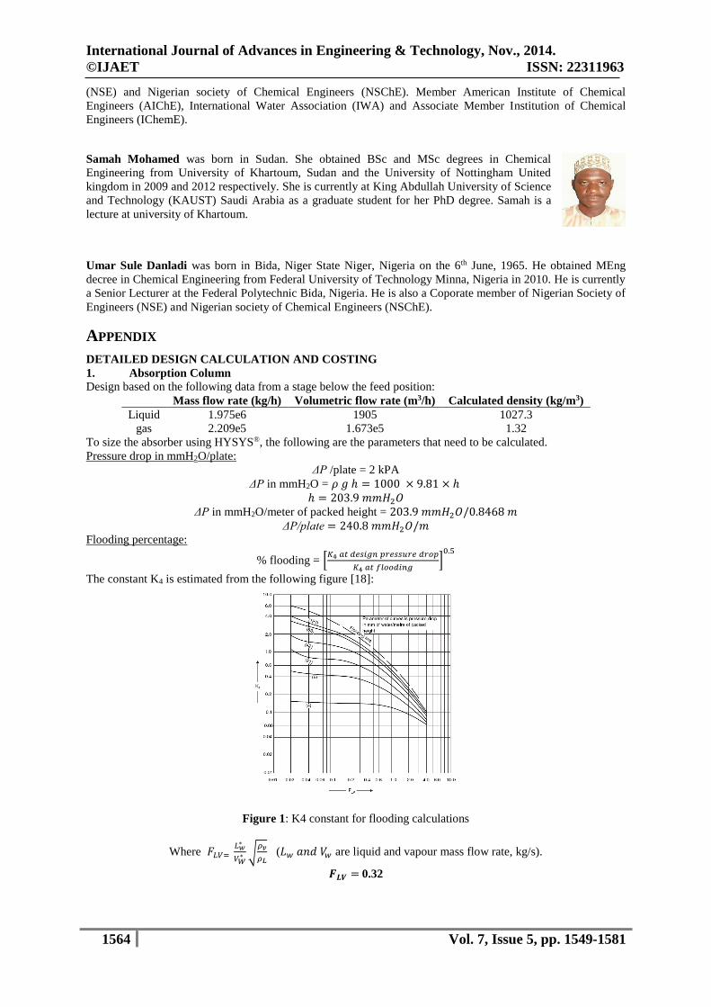
Flooding percentage:

% flooding = [𝐾4 𝑎𝑡 𝑑𝑒𝑠𝑖𝑔𝑛 𝑝𝑟𝑒𝑠𝑠𝑢𝑟𝑒 𝑑𝑟𝑜𝑝

𝐾4 𝑎𝑡 𝑓𝑙𝑜𝑜𝑑𝑖𝑛𝑔]

0.5

The constant K4 is estimated from the following figure [18]:

Figure 1: K4 constant for flooding calculations

Where 𝐹𝐿𝑉= 𝐿𝑤

∗

𝑉𝑊∗ √

𝜌𝑣

𝜌𝐿 (𝐿𝑤 𝑎𝑛𝑑 𝑉𝑤 are liquid and vapour mass flow rate, kg/s).

𝑭𝑳𝑽 = 0.32



1565 Vol. 7, Issue 5, pp. 1549-1581

From the graph at 𝐹𝐿𝑉= 0.32 and 240.8 𝑚𝑚𝐻2𝑂/𝑚 curve

𝑭𝑳𝑽 Curve K4

At design pressure drop 0.32 240.8 mmH2O/m 1.3

At flooding 0.32 (Flooding curve) 1.8

% flooding = [𝐾4 𝑎𝑡 𝑑𝑒𝑠𝑖𝑔𝑛 𝑝𝑟𝑒𝑠𝑠𝑢𝑟𝑒 𝑑𝑟𝑜𝑝

𝐾4 𝑎𝑡 𝑓𝑙𝑜𝑜𝑑𝑖𝑛𝑔]

0.5

= 84.98%

Cost estimation:

Wall thickness is calculated (Sinnott, 2005): 𝑡 =𝑃𝑖𝐷𝑖

2𝑆−𝑃𝑖

Where, 𝑃𝑖 is the internal pressure, and

S is the maximum allowable stress (For stainless steel = 20 ksi = 1.397.5 kPa)

t = 0.0054m (adding 2mm for corrosion allowance)

The cost formula used [18]:

Cost = a + b.Sn

a b N S S* Cost

Vessel 15000 68.00 0.85 Shell mass (kg) 19.8e3 kg 3.205e5

Packing 0.0 1800 1.00 Volume (m3) 2675 4.186e6

Total Cost £/year £5.136e6

*S calculations:

Shell mass = 𝜋𝐷𝐿𝑡𝑤𝜌 = 19.8e3 kg [𝜌 = metal density (8000kg/m3)]

Packing volume = 𝜋𝑟2𝐿 = 2675 m3

Cost for 8 columns = £5.136e6 × 8 = £41.08 million

Cost at (2011) using Table II-3 = £50.94 million

2. Stripper Column

Design based on a stage below the feed position:

Mass flow rate (kg/h) Volumetric flow rate (m3/h) Calculated density (kg/m3)

Liquid 2.077e6 2605 1005.8

gas 1.333e5 1.11e5 1.2

To size the absorber using HYSYS®, the following are the parameters that need to be calculated.

Flooding percentage:

Assume 85% flooding initially

Thus actual real flooding [18]:

Flooding % = 𝑈𝑛

∗

𝑈𝑓

Flooding velocity = 𝑈𝑓 = 𝐾1∗ √

𝜌𝐿−𝜌𝑣

𝜌𝑣

K1 obtained from the graph [18]:

Figure 2: K4 constant for flooding calculations



1566 Vol. 7, Issue 5, pp. 1549-1581

Where 𝐹𝐿𝑉= 𝐿𝑤

𝑉𝑤√

𝜌𝑣

𝜌𝐿 (𝐿𝑤 𝑎𝑛𝑑 𝑉𝑤 are liquid and vapour mass flow rate, kg/s).

FLV = 0.54

Plate spacing is assumed = 0.6096 m

From the graph:

K1 = 0.058

Corrected 𝐾1∗ = 𝐾1 [

𝜎

0.02]

0.2

[𝜎 is the liquid surface tension]

𝐾1∗= 0.069

Flooding velocity = 𝑈𝑓 = 𝐾1∗ √

𝜌𝐿−𝜌𝑣

𝜌𝑣 = 1.996 m/s

Thus, the velocity 𝑈𝑛 = 𝑓𝑙𝑜𝑜𝑑𝑖𝑛𝑔% × 𝑈𝑓 = 1.697𝑚/𝑠

The velocity Un = 1.697 m/s

After sizing the velocity = 𝑈𝑛∗ =

𝑓𝑙𝑜𝑤 𝑟𝑎𝑡𝑒

𝑐𝑟𝑜𝑠𝑠 𝑠𝑒𝑐𝑡𝑖𝑜𝑛𝑎𝑙 𝑎𝑟𝑒𝑎 =

(1.11𝑒5/3600)

𝜋32 = 1.1𝑚/𝑠

Thus, actual flooding % = 𝑈𝑛

∗

𝑈𝑓 = 65%

Cost estimation:

Wall thickness is calculated [18]: 𝑡 =𝑃𝑖𝐷𝑖

2𝑆−𝑃𝑖

Where, 𝑃𝑖 is the internal pressure, and

S is the maximum allowable stress (For stainless steel = 15 ksi = 1.034e5 kPa)

t = 0.0085m (adding 2mm for corrosion allowance)

The cost formula used [18]:

Cost = a + b.Sn

a b N S S* Cost

Vessel 15000 68.00 0.85 Shell mass (kg) 2.359e4 kg 3.693e5

Trays 110.0 380.0 1.80 Diameter (m) 6 1.039e4×30

Total Cost £/year £6.811e5

*S calculations:

Shell mass = 𝜋𝐷𝐿𝑡𝑤𝜌 = 2.359e5 kg [𝜌 = metal density (8000kg/m3)]

Cost for 8 columns = 6.811e5 × 8 = £5.449 million

Cost at (2011) using Table II-3 = £6.76 million

3. Compressors

Compressors are needed in the process flow sheet for pumping the gas streams through the absorbers and finally

to increase the pressure of the carbon captured in order to store it underground. As these two processes are well

distinguished for the pressure range allowed, it is possible to use Figure 3 and Table 1 in order to define each

type of compressor.

Figure 3: Compressor Operating ranges for selection [18, pp. 477] and [24 pp. 1]



1567 Vol. 7, Issue 5, pp. 1549-1581

Table 1: Operating ranges for compressors and blowers from [18]

Type of Compressor

Normal maximum

speed

Normal maximum

capacity

Normal maximum pressure

(differential) (bar)

(rpm) (m3/h) Single stage Multiple stage

Displacement

1. Reciprocating 300 85,000 3.50 5000

2. Sliding Vane 300 3,400 3.50 8

3. Liquid Ring 200 2,550 0.70 1.7

4. Rootes 250 4,250 0.35 1.7

5. Screw 10,000 12,750 3.50 17

Dynamic

6. Centrifugal Fan 1,000 170,000

0.2

7. Turbo Blower 3,000 8,500 0.35 1.7

8. Turbo compressor 10,000 136,000 3.50 100

9. Axial flow fan 1,000 170,000 0.35 2

10. Axial flow blower 3,000 170,000 3.50 10

Taking the volumetric flow rate at the inlet of the absorbers, we have:

QAct = 1,350.182 m3/h

To establish the pressure of this stream, it is necessary to analyze the absorbers and their outlets and recalculate

back the necessary pressure to overcome the head losses caused by the packing material. A pressure drop of 2

kPa/stage and an atmospheric outlet for the sweet gas were assumed for the gas through the absorbers.

Accounting for 30 stages in the absorption operation,

Pinlet Abs = Poutlet + ΔPAbsorption

ΔPAbsorption = NStages * ΔP [kPa/stage]

= (30 * 2) kPa

=60 kPa

Poutlet = 100 kPa (atmospheric)

Pinlet Abs = 100 kPa + 60 kPa

Pinlet Abs = 160 kPa

From Table 4-1, it is possible to get the pressure of the flue gas coming from the power plant and therefore a

pressure increase can be calculated for this compressor,

Pflue Gas = 110 kPa

ΔP Compressor = Pinlet Abs – Pflue Gas = (160 – 110) kPa

ΔP Compressor = 50 kPa = 0.5 bar

By using these values in Figure 3 and Table 1, it can be seen that only dynamic compressors can fit the process

conditions because of their high volumetric flow rate and low differential pressure. It is also possible to realize

that several blowers in parallel are needed in order to achieve the total volumetric flow rate and therefore data

for the maximum actual capacity of blowers is needed. From Figure 3 and considering the limitations for these

data [25]:

Centrifugal Compressors

Axial (inline) centrifugal gas compressor with motor driver. Excludes intercoolers and knock-out drums.

Design Basis Simulation Conditions

Year 1st Quarter 1998 Dollars Nov 2011 (last CEPCI available)

Material Carbon Steel Carbon Steel

Inlet Temperature 68 F 122 F

Inlet Pressures 14.7/ 14.7/ 190 psia 15.95 psia

Pressure Ratios 3:1/ 10:1/ 10:1 1.5:1

Molecular Weight 29 30.03

Specific Heat Ratio 1.4 1.38

Cost estimation:



1568 Vol. 7, Issue 5, pp. 1549-1581

With exception to the higher inlet temperature and the low pressure ratio suggesting that no multiple stages are

required, this equipment seems to fit all the process conditions to calculate accurately the cost. In the case of this

simulation, the installed cost was taken from Table 2, source for Figure 4 and finally these costs will be brought

to present according to the last Chemical Engineering Plant Cost Indexes available, shown in Table 3.

Figure 4: Cost plot for centrifugal compressors [25]

Table 2: Data for constructing Figure 4. [25]

Actual Capacity Purchased

Equipment Cost Installed Cost

(cfm) (USD) (USD)

500 595,400 702,700

1,000 626,400 749,300

5,000 719,700 907,100

10,000 1,114,800 1,339,000

50,000 2,699,800 3,247,700

100,000 5,275,800 6,142,000

150,000 8,722,600 9,735,100

200,000 9,627,600 10,980,400

Table 3: Chemical Engineering Plant Cost Indexes CEPCI [26]

Year CE Index

1998 389.5

2001 394.3

2004 444.2

2005 468.2

Nov 2011 550.8

From Table 2, the maximum volumetric flow rate available for costing is:

Qmax = 200,000 ft3/min = 339,802 m3/h

Therefore, the number of compressors in parallel required is given by:



1569 Vol. 7, Issue 5, pp. 1549-1581

Number of compressors needed = QAct / Qmax = 1,350,182 / 339,802

= 3.973 ~ 4 Compressors

Actual Number of compressors = Compressors needed + 1 (spare equipment)

Actual number of compressors = 5 Compressors

Flow rate per compressor = QAct/#Compressors

=1,350,182 / 4

Flow rate per compressor = 337,545 m3/h = 198,672 cfm

Cost per installed compressor = 10,947,320 USD (interpolated from Table 2)

Total cost of compressors = 10.95 million USD * 5 = 54.74 million USD (1998)

Total cost to present = 54.74 m USD * (550.8/389.5)*(1£/1.571USD)

Total Capital Cost = 52.85 million £

It is also possible to estimate and input into the simulation the polytropic efficiency for a compressor with a

determined inlet flow rate by reading the y-axis in Figure 5 as follows,

Suction flow rate = 1,739,485 m3/h (from Aspen HYSYS simulation)

Suction flow rate = 255,956 acfm

Actual Polytropic Efficiency: 0.8257 (read from Fig. 5)

Figure 5: Approximate polytropic efficiencies for centrifugal and axial-flow compressors [24]

Taking the power requirements for the compressor from the simulation in Aspen HYSYS and applying the data

from literature:

Power price: 0.05 $/kW.h [27]

Power Consumption: 25,296 kW (from Aspen HYSYS simulation)

CO2 Captured = 445.56 tons/h (from Aspen HYSYS simulation)

Power Cost = 0.05 USD/kW.h * 25,296 kW * (1£/1.571USD) * (550.8/468.2)

Power Cost = 947.13 £/h

Power Cost = 2.13 £/ton CO2 Captured

4. Pumps

These are necessary in the process flow sheet to move the absorbent solution through the pipelines and other

major pieces of equipment where high pressure drops are present, such as heat exchangers and filters. Tall



1570 Vol. 7, Issue 5, pp. 1549-1581

towers do not offer losses due to friction but for static head that has to be overcome in order to distribute the

liquid at the top of the equipment.

The most common used pumps are centrifugal and these can be selected according to the flow rate and the total

head according to Figure 6

Figure 6: Guideline for Centrifugal pump selection [18] pp. 200.

The materials for pumps construction and other major pieces of equipment have to be resistant to corrosiveness

and some authors [28] have suggested that stainless steel is suitable for rich amine streams (high CO2 content,

velocities in pipes between 5 – 8 ft/s) and carbon steel can be used for lean amine streams (low CO2 content,

maximum velocity in pipes 3 ft/s), in addition, the velocity of the fluid must be considered for amine solutions

flowing through pipes to avoid further damage for erosion and corrosion effects. Thus, the pump design is

intrinsically related to the pipelines design not only for accounting for friction losses but for materials of

construction, velocities and heights of interconnected pieces of equipment as well.

Recycled Amine pump:

Taking the flow rate from the simulation,

Q = 16,223 m3/h

Despite the CO2 load (and implicitly the corrosiveness) of this steam is the lowest in all the flow sheet, this point

of the process is the one with the greatest erosion effects due to the stream solids content because it includes the

microfiltration equipment inlet (where solids are collected and removed from the stream) so stainless steel

piping will be used in this and every other point of flow of amine in the system. In order to keep the velocity in

the range suggested by the literature as discussed before, the area for the flow and therefore the pipe diameter

should be:

v = 7 ft/s (2.134 m/s) Velocity chosen

Aflow = Q / v = (16.223 m3/h) / (2.134 m/s) = π.D2/4

D = 0.82 m ~ 32.3 in

Before a centrifugal pump type can be chosen from Figure 6, it is necessary to calculate the total head required

and therefore an estimation of pressure drops from pipelines and heights of the different equipment must be

done. For this purpose, it is assumed to have a plant as shown in Figure 7 below where the distance between

connected equipments was set to 1.5 times the biggest dimension of both in the attachment direction, allowing

for maintenance/replacement if necessary.

Table 4: Accessories in Figure 7 for friction loss determination in Lean Amine pump

ACCESSORIES Equivalent

Diameters

BEFORE PUMP AFTER PUMP

# Eq. Length (m) # Eq. Length (m)

Pipelines Length (m) - 213.5 213.5 109.8 109.8

90° standard long elbow 23 2.0 37.7 2.0 37.7

Tee-entry from leg 60

4.0 196.8

Tee-entry into leg 90 9.0 664.2 12.0 885.5



1571 Vol. 7, Issue 5, pp. 1549-1581

Union and coupling 2 5.0 8.2 6.0 9.8

Sharp reduction (tank outlet) 25 8.0 164.0

Sudden expansion (tank inlet) 50

8.0 328.0

TOTAL EQUIVALENT LENGTH

1087.6

1567.6

Total length (L) = 1087.6 m + 1567.6 m = 2655 m

To calculate the friction losses it is necessary to apply [18]:

ΔPf = 8.f.(L/D)(ρv2/2)

Where,

ρ = 1027.9 kg/m3 (taken from the simulation)

µ = 1.55 cP (taken from the simulation)

Absolute roughness = 0.046 mm (taken from Sinnott, 2005 [18], pp 202)

Pipe roughness = Absolute roughness/Diameter = 4.6x10-5 / 0.82 = 5.61x10-5

Pipe roughness ~ 0.0001

Re = ρvD/µ= 1,157,597 ~ 1.16 x 106

f = 0.0016 (read from Figure 7)

Then,

ΔPf = 96.97 kPa

Taking from the simulation the pressure drops for the flow of the solution through the heat exchangers and

microfilters,

ΔPeq = ΔPH.E + ΔPCOOLER+ΔPMICROFILTER

ΔPeq = 65 kPa + 50 kPa + 335.2 kPa

ΔPeq = 450.2 kPa

To calculate the static head necessary to take the fluid from the bottom of the stripper to the top of the absorbers

for recycling, it is necessary to check Figure 6 to get:

ΔPh = ρg. Δh = 1027.9 kg/m3 * 9.81 kg/m.s2 * (26-1) m

ΔPh = 252.1 kPa

The total head to define the type of pump from Fig.6 is defined by,

h (m) = (ΣΔPi)/ρ.g = (96.97 + 450.2 + 252.1)/(1027.9 * 9.81) m

h = 79.27 m

And the number of pumps required from the process flow sheet is 3, so the flow per pump is:

Qp = Q / 3 = 4056 m3/h

Type of Pump: Single Stage (1750 rpm)

It must be noticed that the number of pumps do not affect the calculations made for the pressure drop based on

the initial volumetric flow rate because the flow is only divided to feed the microfilters and it is converged into

one stream after the microfiltration systems. To calculate the specific speed commonly used by pump

manufacturers, and define the type of impeller:

𝑁′𝑠 = 1.73 𝑥 104 𝑁𝑄1/2

(𝑔ℎ)3/4

Where,

N = revolutions per second (1750 rpm)

Q = flow, m3/s (4056 m3/h)

h = head, m (79.3 m)

g = gravitational acceleration m/s2 (9.81 m/s2)

And using the appropriate units,

N’s = 7274 rpm

The pump impeller type can be defined from Table 5 as:

Table 5: Different types of Impellers

Type of Impeller Specific Speed

Radial 400 - 1000

Mixed Flow 1000 - 7000

Axial > 7000

Type of Impeller: Axial



1572 Vol. 7, Issue 5, pp. 1549-1581

Figure 7: Fanning factor for friction pressure drop calculations [18]

Cost estimation

Single and multistage centrifugal pumps for process or general service when flow/head conditions exceed

general service. Split casing not a cartridge or barrel. Includes standard motor driver.

Design Basis Simulation Conditions

Year 1st Quarter 1998 Dollars Nov 2011 (last CEPCI available)

Material Carbon Steel Stainless Steel

Design Temperature 120 F 117 F

Design Pressure 150 psig 111 psia

Liquid Specific Gravity 1 1.03

Efficiency <50 GPM = 60% 17,859 GPM = 82%

50 – 199 GPM = 65%

100 – 500 GPM = 75%

> 500 GPM = 82%

Driver Type Standard motor

Seal Type Single mechanical seal

With exception to the material of construction which can be corrected with an appropriate factor, this

description fits all the process conditions to calculate accurately the cost. The installed cost was taken from

Table 6. with extrapolation and using the 0.6 rule, and finally these costs will be brought to present according to

the last Chemical Engineering Plant Cost Indexes available, shown previously in Table 3.

Table 6: Costing data for centrifugal pumps [25]

Actual

Capacity

Purchased

Equipment

Cost

Installed

Cost

(gpm) (USD) (USD)

3,000 15,200 58,100

4,000 19,500 72,300

5,000 23,800 77,100

6,000 28,400 93,400

7,000 37,800 103,000

8,000 41,300 119,700

9,000 47,300 126,200

10,000 51,200 144,800



1573 Vol. 7, Issue 5, pp. 1549-1581

From Table 6, the maximum volumetric flow rate available for costing is:

Qmax = 10,000 gpm = 2271 m3/h

Which is less than the actual flow rate required (4056 m3/h).

Therefore, by using the 0.6 rule for the actual volumetric flow rate per pump:

Extrapolated Cost = Max Cost*(4056/Qmax)0.6

Extrapolated Cost =144,800 * (4056/2271)0.6

Cost per installed Pump = 0.2051 million USD

Actual Number of pumps = Pumps needed + 1 (spare equipment)

Actual number of pumps = 4 Pumps

Total cost of pumps = 0.2051 million USD * 4 = 0.8204 million USD (1998)

Total cost to present = 0.8204 m USD * (550.8/389.5)*(1£/1.571USD)

Partial Total Capital Cost = 0.8202 million £

Total cost corrected by Material = Total cost * Correction factor (S.S. 316)

Total cost corrected by Material =0.8202 m£ * 1.8 [25] pp. 45

Total Capital Cost = 1.426 million £

Taking the power requirements for the pumping process from the simulation in Aspen HYSYS and applying the

data from literature:

Power price: 0.05 $/kW.h [27]

Power Consumption: 4,002 kW (from Aspen HYSYS simulation)


Power Cost = 0.05 USD/kW.h * 4,002 kW * (1£/1.571USD) * (550.8/468.2)

Power Cost = 149.84 £/h

Power Cost = 0.336 £/ton CO2 Captured

5. Microfilter Design

This step is necessary to remove the solids coming from the flue gas that were scrubbed during the absorption

and those formed during the degradation process of the amine. This equipment is suitable for treatments with

amines at temperatures over those present in the simulation and therefore complies with the necessary

specifications to fit the purpose.

The flow rate across the filter will be the recycled stream with the following characteristics (taken from the

simulation in Aspen-HYSYS):

Total Q = 16,449 m3/h (72430 gpm / 104.3 mgd / 4345.8 kgal/h)

Temperature = 47 ºC

µ = 1.544 cP

Specific Gravity (SG) = 1.014

Using HDC II filter,

Qmax = 30500 gpm

Housing ΔP = 0.3*SG [bar] - Pall, 19 HDC II Medium 80 in length cartridges

Cartridges ΔP = 0.12*µ [mbar/(m3/h)] - Pall, HDC II Medium 80 in length

Maximum Pressure Drop Allowed = 3.44 bar @ 82 ºC

Then,

Number of Microfilters Required = Total Q / Qmax

Number of Microfilters Required = 2.37 ~ 3

Actual Number of Microfilters = Number of Microfilter Required + 1 (Spare Equipment)

Actual Number of Microfilters = 4 systems

Number of cartridges = 19 (cartridges/housing) * 4 systems= 76 Cartridges

ΔP Housing = 30.41 kPa

ΔP Cartridges = 304.8 kPa

Total ΔP = 335.2 kPa (3.35 bar ok!)

Cost estimation:



1574 Vol. 7, Issue 5, pp. 1549-1581

According to literature [29], cost estimation can be made depending on the necessary flow rate according to

Figure 8:

Figure 8: Cost estimation for microfiltration according to flow rate [29] pp. 3.

According to the flow rate (Q) from the simulation and assuming the last available cost according to the curve in

Figure 8,

Cost of microfiltration ~ 33 cents/kgal (read)

Cost of microfiltration = 0.33 USD/kgal * 4345.8 kgal/h * (590.8/394.3) / 1.571 USD/£

(CEPCI taken from Table AIII)

Cost of Microfiltration = 1368 £/h


Cost of Microfiltration = 3.07 £/Ton CO2

6. Heat Exchangers

The calculations were exported from variables in Aspen Hysys.

Table 7: Heat exchanger conditions

Shell side conditions





Tube side conditions





The type of heat exchanger is U-tube bundle.

The overall heat transfer coefficient, U and the parameter UA where A is the area:

Table 8: U and UA

Overall U kJ/h m2 oC 4888565.07

UA kJ/h oC 294871298.39



1575 Vol. 7, Issue 5, pp. 1549-1581

The area for heat transfer is 60.32 m2.

The shell and tube material is stainless steel.

Figure 9: Correlation for heat exchanger cost [18] pp. 254

The purchase cost of the heat exchanger is given by the formula:

𝑃𝑢𝑟𝑐ℎ𝑎𝑠𝑒𝑑 𝑐𝑜𝑠𝑡 = (𝑏𝑎𝑟𝑒 𝑐𝑜𝑠𝑡 𝑓𝑟𝑜𝑚 𝑓𝑖𝑔𝑢𝑟𝑒) × 𝑇𝑦𝑝𝑒𝑓𝑎𝑐𝑡𝑜𝑟 × 𝑃𝑟𝑒𝑠𝑠𝑢𝑟𝑒 𝑓𝑎𝑐𝑡𝑜𝑟

From the Figure 9, the capital cost is £50,000.

Capital cost as of 2004 is £42,500.

To update the cost, the annual index:

As of 2004 As of Nov 2011

444.2 686.6

Therefore, the cost of the heat exchanger in 2012 is £65,692.3. To convert the cost into £/h, one year with an

operational period of 8000 hours is assumed. Therefore, cost per hour in a year is 8.2 £/h.

7. Cooler Design

Table 9: Cooler conditions

Shell side conditions (CO2 lean solvent)



Temperature oC 25 25


Tube side conditions (Cooling water)




Pressure kPa 150 100

The type of heat exchanger is U-tube bundle.

The overall heat transfer coefficient, U and the parameter UA where A is the area:

Overall U 1448758.50

UA 87387053.92

The area for heat transfer is 60.32 m2.

The shell and tube material are carbon steel and stainless steel respectively.



1576 Vol. 7, Issue 5, pp. 1549-1581

From Figure 9, the purchase cost of the cooler is £37,000.

The cost as of 2004 is £31,450. The updated cost of the cooler as of 2012 is £48,612.30. To convert the cost into

£/h, one year with an operational period of 8000 hours is assumed. Therefore, cost per hour in a year is 6.1 £/h.

8. Stripper Condenser Design

The condenser operates at full reflux with a negligible pressure drop.

Table 10: Flows involving condenser

Flow into condenser kg/h 960514.75

Flow out of condenser kg/h 454175.65

Reflux kg/h 506339.10

The heat transferred, Q is 1.308E+09 kJ/h.

The UA parameter is exported from Aspen Hysys and was found to be 360000 kJ/ oC h. The estimated U was

found from Coulson & Richardson’s Chemical Engineering and Design, from the following table:

Table 11: Estimated U values [18]

The overall heat transfer coefficient, U was found to be 3060 kJ/h m2 oC.

The inlet and outlet temperatures of the condenser are given by:

Condenser Inlet 103.43

Condenser Outlet 38.28

Assuming cooling water as the cooling agent with an inlet temperature of 25 oC and a maximum temperature

increase of 20oC, the mass of water required is:

𝑚 =𝑄

𝐶𝑝∆𝑇

The specific heat capacity of 4.2 kJ/kmol oC was used. Hence, mass of water is 6.92E+06 kg/h. The driving

force of the heat exchanger was found to be 30.48oC and therefore, the area for heat transfer was found to be

117.6 m2.

The type of heat exchanger is a shell and tube heat exchanger where the material of the shell and tube are carbon

steel and stainless steel respectively.

The purchase cost found was and as of 2004, £160,000. The estimated cost in 2012 is £247,300 and cost per

hour in a year of 30.91 £/h.



1577 Vol. 7, Issue 5, pp. 1549-1581

9. Reboiler Design

The type of reboiler is a kettle reboiler.

The heat transferred, Q is 2.87E+09 kJ/h.

Table 12: Flows involving reboiler

Flow into reboiler kg/h 17972649.79

Flow out of stripper bottoms kg/h 16675110.21

Total flow out kg/h 34647759.99

From Table 11, estimated U is 5400 kJ/h m2 oC.

The temperatures involving the boiler are:

Tempearture into boiler oC 123.07

Temperature in boiler oC 123.72

Steam enters the system at 3 bar. The saturation temperature is 133.5 oC.

The LMTD found was 10.10oC. Therefore, the area for heat transfer is 52,640 m2. The capital cost found as of

2012 is £26,440,000 with a cost/hour in a year of 3305 £/h. This can be improved by using steam at a higher

pressure and temperature.

ENERGY REQUIREMENTS

Heating

The only piece of equipment with calorific energy requirement in the process flow diagram is the reboiler in the

stripper, the variables associated are (taken from the simulation in Aspen-HYSYS):

Reboiler Heat = 2’870,174 MJ/h

Reboiler Temperature = 123.7 ºC

The easiest way to supply this amount of energy in a reboiler is by using saturated steam and the appropriate

temperature should assure a high heat transfer coefficient. The temperature approach assumed for the process

will be used to calculate the minimum temperature and therefore pressure for the steam required as follows,

Temperature Approach = 7 ºC (Assumed)

Min. Temperature of steam = Temperature of reboiler + Temperature Approach

Min. TSteam = 123.7 ºC + 7 ºC = 130.7 ºC

Psat131ºC = 279.6 kPa ~ 3 bar (Taken from Aspen-HYSYS)

λvap3 bar = 2191.4 MJ/ton (Taken from Aspen-HYSYS)

Steam Flow rate = Reboiler Heat / λvap3 bar

Steam Flow rate = 1310 ton/h

Cost Estimation

By using the data found in the literature [27], the cost of this steam will be:

Type of Steam = Low Pressure Steam (L.P. Steam 3 bar)

Price of L.P. Steam = 0.17 USD/ton (2005)

Now, by using the CECPI in Table 3 and the exchange rate for USD:

Cost of Steam = Steam Flow rate * Price of Steam * Correction factors

Cost of steam = 1310 ton/h * 0.17 USD/ton * (590.8/468.2) / (1.571 USD/£)

Cost of Steam = 178.8 £/h

(CO2 Captured = 445.56 ton/h)

Cost of Steam = 0.4013 £/ton CO2

Cooling

There are three streams that need to be cooled down during the process but as it will be seen, only one coolant

stream is necessary due to the possibility of heat exchanger nets (HEN) that can be applied and the difference in

temperature of the different processes.

a. Cooling for condenser in Stripper



1578 Vol. 7, Issue 5, pp. 1549-1581

Taking the values of the process variables from the simulation (Aspen-HYSYS) and assuming a water

temperature between 25-30ºC (25 ºC used in this case),

Heat to remove = 1’307,881 MJ/h

Condenser Temperature = 38.4 ºC

Inlet Water Temperature = 25 ºC (from cooling tower)

Cp (water) = 4.126 kJ/kg.ºC

Temperature Approach = 7 ºC

Water Outlet Temperature = Condenser Temperature - Temperature Approach

Water Outlet Temperature = 31.4 ºC

Water ΔT = (31.4 – 25) ºC

Heat = Flow rate * Cp * ΔT

Water Flow rate = Heat / (Cp * ΔT)

Water Flow rate = 49,873 ton/h

b. Cooling for recycled DEA stream

Once again, the variables in the process are (from Aspen-HYSYS simulation),

Heat to remove = 1’540,199 MJ/h

DEA inlet Temperature = 71.15 ºC

DEA outlet Temperature = 46.9 ºC

Inlet Water Temperature = 31.4 ºC (from condenser)


Temperature = DEA outlet Temperature - Temperature Approach

Water Outlet Temperature ~ 39.9 ºC

Water ΔT = (39.9 – 31.4) ºC

Heat = Flow rate * Cp * ΔT

Water Flow rate = Heat / (Cp * ΔT)

Water Flow rate = 43,916 ton/h

c. Cooling for inter-stage Compression for carbon storage

The heat to be removed to improve the compression efficiency is (from Aspen-HYSYS simulation),

Heat to remove = 141,604 MJ/h

Inlet Water Temperature = 31.4 ºC (from condenser)


Water flow rate still available = Water for condenser – Water for DEA cooling

Water flow rate still available = (49,873 – 43,916) ton/h = 5957 ton/h

∆T = Heat / (Flow rate * Cp) = 5.8 ºC

Water outlet Temperature = Water Inlet Temperature + ∆T = (31.4 + 5.8) ºC

Water outlet inter-stage temperature = 37.2 ºC (Suitable!)

As seen in these calculations, the water from the condenser is enough for both DEA cooling and CO2

compression inter-stage cooling, so the cost can be estimated as:

Price of Water from Cooling Towers = 0.015 £/ton (2004)

Water Flow rate required = 49,873 ton/h

Cost of Cooling water from Towers = 995 £/h (Nov 2011)

Cost of Cooling water from Towers = 2.23 £/ton CO

CAPITAL AND OPERATING COST CALCULATIONS:

Total Capital Investment:

Total Capital investment (TCI) = Fixed capital investment (FCI)+Working capital (WC)

(TCI) = FCI + 10% TCI

(FCI) = Total equipment cost (TEC) + Direct cost (DC) + Indirect cost (IC)

= £372,437,287.29

Total Capital investment (TCI) = £372,437,287.29 + 10% of TCI = £413,819,208.1053

Adding the initial raw material cost (DEA and water): (TCI) = £417,974,468.1053

Total Product Cost: Total product cost (TPC) = Manufacturing cost (MC) + General expenses (GE)

(TPC) = (MC) + (9% TPC)

(MC) = Direct product cost (DPC) + Fixed charges (FC) + Plant overhead cost (POC)

= (Direct product cost (DPC) +Raw material cost) + Fixed charges (FC) + (5% TPC)

£111,512,670.4687



1579 Vol. 7, Issue 5, pp. 1549-1581

Total Annual Cost:

Total cost per year = Total product cost + Energy cost + Abatement cost + Geological sequestration cost =

£147,258,623.7395

Total cost per year:

The capital recovery (equivalent annual cost for the total capital investment):

𝐴 = 𝑃 × [𝑖 (1 + 𝑖)𝑛

(1 + 𝑖)𝑛 − 1]

Where P = £417,974,468.1053, i = 15% and n = 25 years

A = £55,957,911.88

Total cost per year = £196,987,006.8782

The working capital includes the amount of money required for one month production (raw material,

monthly cash on hand, account payable and other costs), it ranges from 10-20% of TCI [30]. It is

assumed as 10% of the total capital investment.

The plant overhead cost include the expenditure required for routine plant services it ranges from 5-

15% of TPC [30]. It is assumed as 10% of the total capital investment.

Tables below summarize the percentages and costs used in the above calculations

Table 13: Total equipment cost

Equipment Total cost

Absorber 4.11E+07

Stripping 5.45E+06

Compressor 8.78E+07

Heat exchanger 1.31E+05

Microfiltration 1.03E+07

Pump 2.55E+06

Sum £152,096,904.00

Table 14: Breakdown of direct cost

Direct cost Assum

ed Comments and (Justifications)

% of fixed capital investment

Purchased equip. 15-40 0 All equipment including spare parts, modifications during start-up.

(Calculated separately in the table above)

% of purchased equipment cost

Installation 25-55 0 Installation of all equipment with supports, insulation, paint

(Included in equipment cost)

Instrumentation &

control 8-50 10

Purchase, installation, calibration, computer tie-in

(high control is required mainly on the columns)

Piping 10-80 20 Process piping, pipe hangers, fittings, valves and insulation

Electrical 10-40 20 Electrical equipment -switches, motors, conduit, wire etc. and

electrical materials

Building 10-70 20 Process buildings - Auxiliary buildings - Maintenance shops -

Building services

Service facilities &

Yard improvement

40-

100 40

Utilities – Facilities - Nonprocess equipment - Distribution and

packaging, Yard: Site development

Land 4-8 4 Surveys and fees and property cost

Sum _ 114

Table 15: Breakdown of indirect cost

Indirect cost Assum

ed Comments and (Justifications)

% of direct cost

Eng.

&supervision 5-30 5 Engineering costs and engineering supervision and inspection

% of fixed capital investment

Legal expenses 1-3 2 Preparing and submission of forms required by regulatory agencies,

contract negotiations

construction

expenses

10-

20 10

Construction, operation, tools and equipment, supervision, accounting,

Safety, medical, Permits, field tests, special licenses, Taxes, insurance,



1580 Vol. 7, Issue 5, pp. 1549-1581

interest

Contractor fee 10-

20 5 (assume 5% because it is a large capital investment project)

Contingency 5-15 10 (High risk project)

Sum _ 27

Table 16: Breakdown of direct production cost

Cost % Assum

ed

Comments and (Justifications)

Operating labour 10-20 of total product

cost 12

Skilled and unskilled labour

Laboratory charges 10-20 of operating labour 1.8 Cost of laboratory tests and quality control. It

depends on labour involved in these tests

Direct supervisory &

clerical labour 10-20 of operating labour 1.8

For Direct supervisory which related to the

operating labour

Utilities 10-20 of total product

cost 5

Electricity, fuel, cooling and heating agent,

waste treatment and disposal, process water

Patents and royalties 0-6 of total Product cost 2 Payment for the use of patent rights or royalty

SUM (1) _ 22.6

Main & repair 2-10 of fixed capital

investment 4

Annual cost for repair equipment (Usually

known as 4% in capture plants)

Oper. Supp. 0.5-1 of fixed capital

investment 0.75

SUM (2) _ 5.75

Table 17: Breakdown of fixed charges

Cost % of fixed capital

investment

Assume

d


Machine

depreciation

10

10

Building

depreciation

2-3

2

Compromise the amount of money that must be paid

pack from the initial investment. Better to be

calculated precisely.

local taxes 1-4

2

Depend on the regional lows and the locality (area

population)

Insurance 0.4-1

0.7

Depend on the process and the available protection

facilities

SUM _ 14.7

Table 18: Breakdown of general expenses

Cost % of total

product

cost

Assume

d


Administrative 2-5 3 executive salaries, clerical wages, computer support, legal

fee, office supplies and communications

Distribution and

marketing 2-20 2 costs for sale office, sales people, shipping and advertising

Research and

development 5 5

Developing of new methods and all cost related to personnel,

equipment, supplies etc.

SUM _ 10



1581 Vol. 7, Issue 5, pp. 1549-1581

Table 19: Energy cost

Energy cost

Material Cost/year

Feed compressor 7577040

Storage compressor 1.61E+07

Stripper feed pump 706880

Microfiltration pump 1198720

makeup pump 2.40E+00

SUM £25,547,842.40

Table 20: Raw material cost

Material Cost

Material Cost/year

DEA 849,600.00

cooling agent 7,960,000.00

steam 1,424,000.00

Makeup water 416,000.00

SUM £10,649,600.00

Table 21: Abatement cost

Abatement cost

Material Amount Cost

discharge cost £1.2/hr £9,600.00

geological sequestration cost £3.18/ton CO2 £11,356,620.40

Net energy calculation:

Energy Cost = £25,547,842.40/year

Energy required = Total energy cost (£/year) / energy cost per (MW.year)

Energy cost per (MW.year) = £840,000.00/(MW.year)

Energy required = 30.41 MW

Net energy produced from the plant at 90% capacity = 500/0.9 = 450 MW

Net energy produced after CCS plant = 450 – 30.41 ≈ 420 MW

technical and economic considerations of … · simulation of the amine absorption post-combustion...

Documents