Technical description of interpolation and processing ofmeteorological data in CGMS

Erik van der Goot, November 1997Stefania Orlandi, December 2003

PREFACE

ACKNOWLEDGEMENTS

1 INTRODUCTION....................................................................................................................5

2 GLOBAL RADIATION CALCULATION................................................................................6

2.1 Introduction.........................................................................................................................................................................6

2.2 Calculation...........................................................................................................................................................................62.2.1 The Angot radiation.......................................................................................................................................................62.2.2 Angot radiation remarks................................................................................................................................................72.2.3 The Ångström formula..................................................................................................................................................82.2.4 The Supit formula..........................................................................................................................................................82.2.5 The Hargreaves formula................................................................................................................................................8

2.3 The regression constants.....................................................................................................................................................92.3.1 Estimation of the regression constants..........................................................................................................................92.3.2 Interpolation of regression constants.............................................................................................................................9

3 CALCULATION OF THE POTENTIAL EVAPORATION.....................................................10

3.1 The Penman formula.........................................................................................................................................................10

4 INTERPOLATION OF DAILY METEOROLOGICAL DATA................................................12

4.1 Interpolation procedure....................................................................................................................................................124.1.1 General selection of weather stations..........................................................................................................................124.1.2 Qualification of weather stations.................................................................................................................................124.1.3 Interpolation of rainfall (and snow) data.....................................................................................................................134.1.4 Interpolation of the other data.....................................................................................................................................144.1.5 Missing data.................................................................................................................................................................14

5 REFERENCES.....................................................................................................................16

APPENDIX A...........................................................................................................................1

2

Preface

This document describes the processing chain used to process daily meteorological data for use withthe Crop Growth Monitoring System (CGMS). The document reflects the state of the software CGMSversion 2.3. Very little of the information in this document is original, and some parts of the text arelifted almost verbatim from the original publications. However, the main purpose of this document is todescribe accurately the current state of the software. For this purpose, a synthesis has been made fromall of the available and relevant documentation and from the program source codes. The differencesbetween the original publications and this document are sometimes subtle, and mainly concern valuesand dimensions of constants. None of the previous publications described the processing chainaccurately, and some implementation details are being documented for the first time.

3

Acknowledgements

CGMS is a complicated system, and before understanding the purpose and requirements of the weatherdata interpolation, it is necessary to have an understanding of the whole CGMS. This is only possiblewhen the few people that fully understand the system are willing to share their knowledge. For thismany thanks are due to Iwan Supit(JRC), Tamme van der Wal (SC-DLO) and Paul Vossen(JRC).Without their support I would have not been able to complete this task.

Erik van der Goot, November 1997.

4

1 Introduction

The final product of the level 1 processing of CGMS is the interpolated daily grid weather. The valuesinterpolated onto the 50*50 km grid are the following:

Value DescriptionMAXIMUM_TEMPERATURE maximum temperature (°C)MINIMUM_TEMPERATURE minimum temperature (°C)VAPOUR_PRESSURE mean daily vapour pressure (hPa)WINDSPEED mean daily windspeed at 10m (m/s)RAINFALL mean daily rainfall (mm)E0 Penman potential evaporation from a free

water surface (mm/day)ES0 Penman potential evaporation from a moist

bare soil surface (mm/day)ET0 Penman potential transpiration from a crop

canopy (mm/day)CALCULATED_RADIATION daily global radiation in KJ/m2/daySNOW_DEPTH daily mean snow depth in cm

It is important to realise that these values are used to describe the ‘average’ conditions prevalent in thegrid cell for this day. They do not necessarily represent the meteorological conditions that could bemeasured at the grid cell centre. Another reason for this is that the altitude value used to describe thegrid cell is not the altitude that can be measured at the grid cell centre, but rather a value that describesthe mean altitude of agricultural activity in the grid cell.

In order to carry out the interpolation of the above-mentioned variables, they need to be available at theweather station level. Unfortunately, the global radiation and the potential evaporation values are notwidely measured or distributed on a regular basis. These values are therefore estimated at the stationlevel, using the available measured meteorological parameters.

This document describes the formula and methods used to estimate global radiation and potentialevaporation and subsequently how the daily meteorological parameters are combined to produce thegrid cell results. This document reflects accurately the state of the software as implemented underWindows NT, November 1997.

5

2 Global radiation calculation

2.1 Introduction

The global radiation calculation is performed using one of three formulae, depending on the availabilityof the meteorological parameters for a station. The calculation is based on work by Iwan Supit asdescribed in ‘Global Radiation, EUR 15745 EN’ and Supit and Van Kappel, ‘A simple method toestimate global radiation (to be published)’.

2.2 Calculation

2.2.1 The Angot radiation

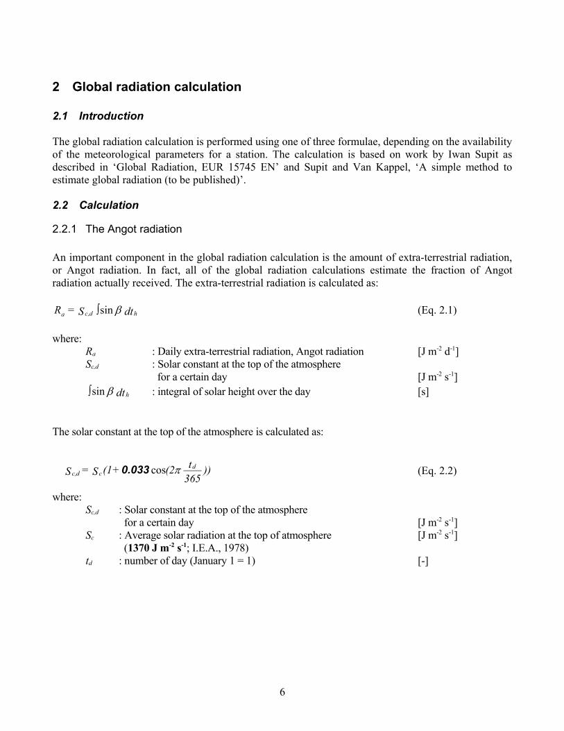
An important component in the global radiation calculation is the amount of extra-terrestrial radiation,or Angot radiation. In fact, all of the global radiation calculations estimate the fraction of Angotradiation actually received. The extra-terrestrial radiation is calculated as:

dt S=R hdc,a βsin∫ (Eq. 2.1)

where:Ra : Daily extra-terrestrial radiation, Angot radiation [J m-2 d-1]Sc,d : Solar constant at the top of the atmosphere

for a certain day [J m-2 s-1]dthβsin∫ : integral of solar height over the day [s]

The solar constant at the top of the atmosphere is calculated as:

))365t(2+(1S=S d

cdc, πcos0.033 (Eq. 2.2)

where:Sc,d : Solar constant at the top of the atmosphere

for a certain day [J m-2 s-1]Sc : Average solar radiation at the top of atmosphere [J m-2 s-1]

(1370 J m-2 s-1; I.E.A., 1978)td : number of day (January 1 = 1) [-]

6

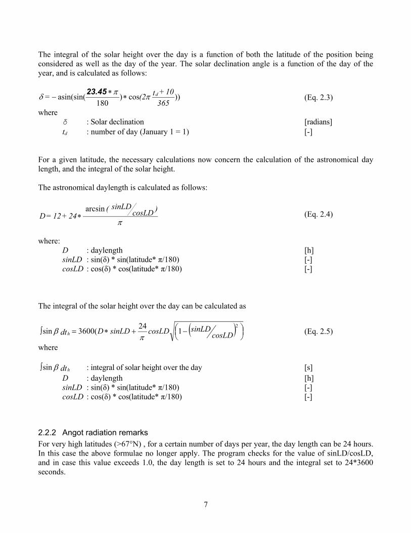
The integral of the solar height over the day is a function of both the latitude of the position beingconsidered as well as the day of the year. The solar declination angle is a function of the day of theyear, and is calculated as follows:

))cos)180

asin(sin(365

10+t(2 = dππδ ∗∗

−23.45

(Eq. 2.3)

whereδ : Solar declination [radians]td : number of day (January 1 = 1) [-]

For a given latitude, the necessary calculations now concern the calculation of the astronomical daylength, and the integral of the solar height.

The astronomical daylength is calculated as follows:

π

)cosLDsinLD (

24 + 12 = Darcsin

∗ (Eq. 2.4)

where:D : daylength [h]sinLD : sin(δ) * sin(latitude* π/180) [-]cosLD : cos(δ) * cos(latitude* π/180) [-]

The integral of the solar height over the day can be calculated as

( )

−+∗=∫

2124(3600sin cosLD

sinLDcosLDsinLDDdth πβ (Eq. 2.5)

where

dthβsin∫ : integral of solar height over the day [s]D : daylength [h]sinLD : sin(δ) * sin(latitude* π/180) [-]cosLD : cos(δ) * cos(latitude* π/180) [-]

2.2.2 Angot radiation remarksFor very high latitudes (>67°N) , for a certain number of days per year, the day length can be 24 hours.In this case the above formulae no longer apply. The program checks for the value of sinLD/cosLD,and in case this value exceeds 1.0, the day length is set to 24 hours and the integral set to 24*3600seconds.

7

2.2.3 The Ångström formula

When the sunshine duration is known, the global radiation is calculated using the Ångström formula,which also relies on two constants that depend on the geographic location.

))/(*(* daaag LnBARR += (Eq. 2.6)

where:Rg : global radiation [J m-2 d-1]Ra : extra-terrestrial radiation (Angot radiation) [J m-2 d-1]Aa, Ba : regression coefficients (Ångström) [-]n : bright sunshine hours per day [h]Ld : astronomical day length [h]

2.2.4 The Supit formula

When the sunshine duration is not available but the minimum and maximum temperature and the cloudcover are known, the following formula is used, which is an extension of the Hargreaves formula. Theregression coefficients depend on the geographic location:

sssag CCCBTTARR +−+−= ))8/1(*)((** minmax (Eq. 2.7)where:

Rg : global radiation [J m-2 d-1]Ra : extra-terrestrial radiation (Angot radiation) [J m-2 d-1]As, Bs : regression coefficients (Supit) [-]Cs : regression coefficients (Supit) [J m-2 d-1]Tmin, Tmax : minimum and maximum daily temperature [°C]CC : Cloud cover in octets [-]

2.2.5 The Hargreaves formula

When only the minimum and maximum temperatures are known, only the first part of the formulaabove is used. Again, the regression coefficients depend on the geographic location:

hhag BTTARR +−= )(** minmax (Eq. 2.8)where:

Rg : global radiation [J m-2 d-1]Ra : extra-terrestrial radiation (Angot radiation) [J m-2 d-1]Ah, Bh : regression coefficients (Hargreaves) [-]Tmin, Tmax : minimum and maximum daily temperature [°C]

8

2.3 The regression constants

2.3.1 Estimation of the regression constantsThe main problem with the application of these formulae is the quality of the regression constants. Thestudy by Supit (1994) shows that in many cases there is no relationship between the latitude and thecoefficients, although such a relation is frequently used to estimate these regression constants.

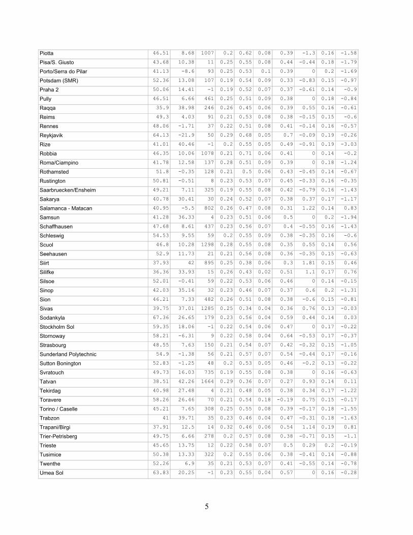
The main purpose of the work by Supit and van Kappel (1994) has been to obtain sets of regressionconstants for the above mentioned formulae for as many weather stations as possible, with a geographicdistribution that corresponds to the area of interest for CGMS. As a result, a set of 256 referencestations has been identified for which a relevant set of measured radiation data and other parameters inthe formulae exist. For these stations the regression constants have been calculated based on measuredradiation data for the three formulae mentioned above (see appendix A).

2.3.2 Interpolation of regression constantsThis body of data, consisting of latitude, longitude, altitude and the regression constants calculated forthe reference stations, is now being used for the derivation of the regression constants for the set ofstations used for the interpolation of the daily meteorological data. This is a process that only has to becarried out once, unless the set of reference stations changes. Once the regression constants have beenestablished for the operational set of stations, the global radiation estimation can proceed using any oneof the above formulae.

The interpolation of the regression constants is based on a simple distance weighted average of thethree nearest stations. For each of the three sets of constants (Ångström, Supit, Hargreaves) a subset iscreated from the complete set of reference stations, by selecting only those stations that have theregression coefficients for the desired method. This subset of stations is then sorted based on distanceto the station for which the regression coefficients are being calculated. This sorting process is alsosubject to an altitude threshold test i.e. if the altitude difference between the target station and areference station is greater than a set threshold the reference station is rejected in favour of the nextnearest reference station. Depending on a distance threshold, the nearest one, two or three stations arethen used to calculate the regression constants. If the threshold tests exclude all stations, the neareststation will be used, regardless of the distance. The altitude threshold value is 200m, the distancethreshold is 200km.

The distance weighted average method used is based on the relative distance of the reference stations tothe station of interest. Assume the distances d0, d1 and d2 to be the distances to the three nearestreference stations, and w0, w1 and w2 the weights to be used in the calculation. As an example, assumethat d1 is 2*d0, then w1 will be w0/2. More general, w1 = w0*d0/d1. Similarly, w2 = w0*d0/d2.Furthermore, the sum of the weights should be 1, so w0+w1+w2 = 1. From the above, the followingrelation can be established:

w0 = d1d2 / (d0d1 + d0d2 + d1d2) (Eq. 2.9) w1 = d0d2 / (d0d1 + d0d2 + d1d2) w2 = d0d1 / (d0d1 + d0d2 + d1d2)

9

3 Calculation of the potential evaporation

3.1 The Penman formula

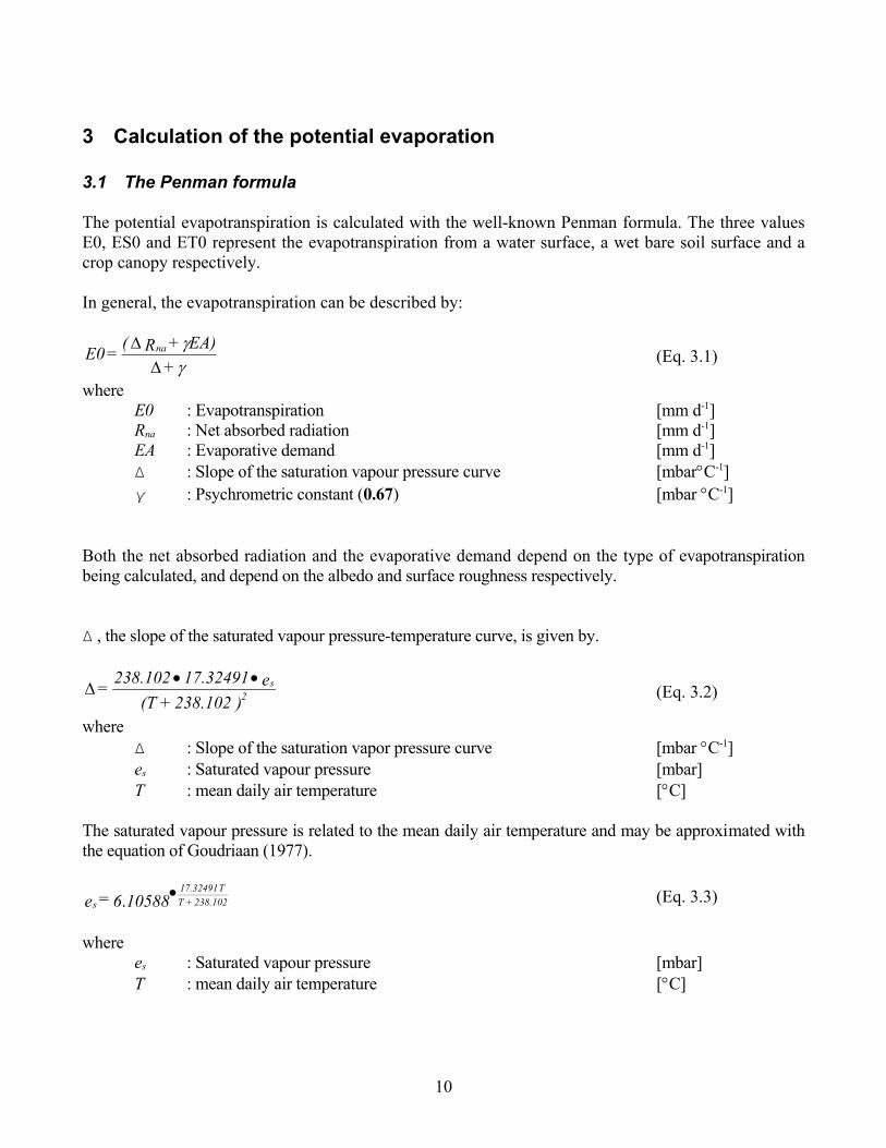
The potential evapotranspiration is calculated with the well-known Penman formula. The three valuesE0, ES0 and ET0 represent the evapotranspiration from a water surface, a wet bare soil surface and acrop canopy respectively.

In general, the evapotranspiration can be described by:

γγ

+ EA) + R( = E0 na

∆∆

(Eq. 3.1)

whereE0 : Evapotranspiration [mm d-1]Rna : Net absorbed radiation [mm d-1]EA : Evaporative demand [mm d-1]∆ : Slope of the saturation vapour pressure curve [mbar°C-1]γ : Psychrometric constant (0.67) [mbar °C-1]

Both the net absorbed radiation and the evaporative demand depend on the type of evapotranspirationbeing calculated, and depend on the albedo and surface roughness respectively.

∆ , the slope of the saturated vapour pressure-temperature curve, is given by.

)238.102 + (Te 17.32491 238.102 = 2

s••∆ (Eq. 3.2)

where∆ : Slope of the saturation vapor pressure curve [mbar °C-1]es : Saturated vapour pressure [mbar]T : mean daily air temperature [°C]

The saturated vapour pressure is related to the mean daily air temperature and may be approximated withthe equation of Goudriaan (1977).

105886 = e 238.102 + TT 17.32491

s . • (Eq. 3.3)

wherees : Saturated vapour pressure [mbar]T : mean daily air temperature [°C]

10

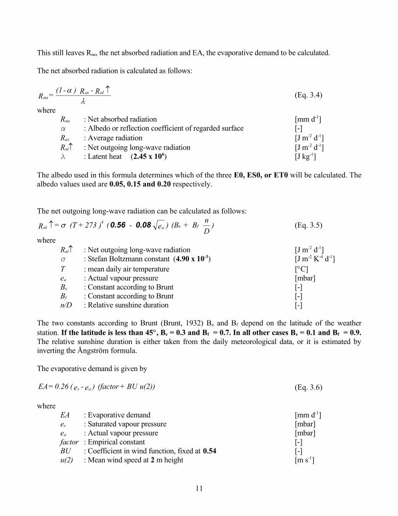
This still leaves Rna, the net absorbed radiation and EA, the evaporative demand to be calculated.

The net absorbed radiation is calculated as follows:

λα ↑R - R ) - (1 = R nlav

na (Eq. 3.4)

whereRna : Net absorbed radiation [mm d-1]α : Albedo or reflection coefficient of regarded surface [-]Rav : Average radiation [J m-2 d-1]Rnl↑ : Net outgoing long-wave radiation [J m-2 d-1]λ : Latent heat (2.45 x 106) [J kg-1]

The albedo used in this formula determines which of the three E0, ES0, or ET0 will be calculated. Thealbedo values used are 0.05, 0.15 and 0.20 respectively.

The net outgoing long-wave radiation can be calculated as follows:

)Dn B + (B )e - ( )273+(T = R fa

4nl e0.080.56σ↑ (Eq. 3.5)

whereRnl↑ : Net outgoing long-wave radiation [J m-2 d-1]σ : Stefan Boltzmann constant (4.90 x 10-3) [J m-2 K-4 d-1]T : mean daily air temperature [°C]ea : Actual vapour pressure [mbar]Be : Constant according to Brunt [-]Bf : Constant according to Brunt [-]n/D : Relative sunshine duration [-]

The two constants according to Brunt (Brunt, 1932) Be and Bf depend on the latitude of the weatherstation. If the latitude is less than 45°, Be = 0.3 and Bf = 0.7. In all other cases Be = 0.1 and Bf = 0.9.The relative sunshine duration is either taken from the daily meteorological data, or it is estimated byinverting the Ångström formula.

The evaporative demand is given by

u(2)) BU + (factor )e - e( 0.26 = EA as (Eq. 3.6)

whereEA : Evaporative demand [mm d-1]es : Saturated vapour pressure [mbar]ea : Actual vapour pressure [mbar]factor : Empirical constant [-]BU : Coefficient in wind function, fixed at 0.54 [-]u(2) : Mean wind speed at 2 m height [m s-1]

11

The following values for factor are assumed (Frère, 1979). For crop canopies (ET0) factor = 1.0 and fora free water surface and for the wet bare soil (E0, ES0) factor = 0.5. This is where the evaporativedemand for E0, ES0 and ET0 is differentiated.

4 Interpolation of daily meteorological data

The interpolation has been implemented following the recommendations of a study carried out by SC-DLO by van der Voet et. Al. (1994). The basis of the interpolation is the selection of the suitable meteorological stations for thedetermination of the representative meteorological conditions for a grid cell. The actual interpolation,once this selection has been made, is in fact a simple average for most of the meteorologicalparameters, corrected for an altitude difference in the case of temperature and vapour pressure. Theexception is the rainfall data, which is taken directly from the most suitable station.

4.1 Interpolation procedure

4.1.1 General selection of weather stationsNot all of the meteorological stations broadcast a complete set of data via the GlobalTelecommunication System (GTS), and not all of the stations are broadcasting all of the time. Toincrease the reliability of the interpolation, and to reduce the computational requirements a number ofchecks is performed on the availability of the data from the weather stations. The first check is basedon a classification with respect to the type of data that the station can deliver. Three classes are beingdistinguished: rainfall data, temperature data and all other data. The second check is based on thetemporal availability of the data in these classes. For the current year the selection of available stationsis simply based on a daily analysis, for historic years the selection procedure determines for eachweather station if the availability for a class of data falls above a certain threshold. If so, then thestation will be marked as a valid station for that type of data. The threshold value can be selected perstation, but is applied to all three categories. A typical example would be a threshold value of 80%, i.e.if the station data in a particular class is available for more than 80% of the time, the station will beused for the interpolation of the data in that class. The timeframe taken into account for the check is thetotal number of days in the year for past years, and the number of days up to the ‘end-of-simulation’day in the current year.

4.1.2 Qualification of weather stationsTo establish the suitability of a weather station for the interpolation, a selection procedure is appliedthat relies on the similarity of the station and the grid centre. This similarity is expressed as the result ofa scoring algorithm that takes the following characteristics into account:

• Distance• Difference in altitude• Difference in distance to coast• Climatic barrier separation

12

The final score is expressed in kilometres and is derived from these geographic characteristics byempirically converting them into kilometres. The higher the score, the less the similarity between thestation and the grid centre.

The score is calculated as follows:

Score = dist + ∆alt*Walt + ∆dCstcorr + ClbInc (Eq. 4.1)

where:dist : distance between the weather station and the grid centre. [km]∆alt : absolute difference in altitude. [m]Walt : weighting factor for ∆alt (= 0.5). [km/m]∆dCstcorr : absolute difference in corrected distance to coast (see below) [km]ClbInc : climate barrier increment. (see below) [km]

The climate barrier increment is set to 1000 when the station and the grid centre are separated by aclimate barrier, otherwise it is set to 0.

The difference in the distance to the coast is expected to be more important when the absolute distanceto coast is small, and of no importance when the actual distance to the coast is large. The empiricalcorrection maps the true distance to coast to a range between 0 and 100 km.

Empirical correction for distance to coast

0

20

40

60

80

100

0 50 100 200 250

True distance to coast (km)

Corr

ecte

d di

stan

ce to

co

ast (

km)

4.1.3 Interpolation of rainfall (and snow) dataIn the current implementation of CGMS precipitation data is not interpolated. The precipitation for agrid is taken from the weather station that is the most similar (as explained above) to the grid centre,i.e. the station with the lowest score. For snow depth the same way is adopted.

13

4.1.4 Interpolation of the other dataAll other data is interpolated using data from up to four stations. To determine which stations to use,and indeed how many stations to use, a combination score is used. This combination score is calculatedin a similar way to the single station score, but is based on the mean values of the combination ofstations.

The set score is calculated as follows:

SetScore = distavg + ∆altavg*Walt + ∆dCstcorravg + DCG + FnS*Scoremin (Eq. 4.2)

where:distavg : average distance between the stations and the grid centre [km]∆altavg : average of the absolute difference in altitude [m]Walt : weighting factor for ∆altavg (=0.5) [km/m]∆dCstcorravg : average of the absolute difference in corrected distance to coast [km]DCG : distance between the grid centre and the centre of gravity

of the set of stations [km] FnS : factor based on the number of stations in the set (see below) [-]Scoremin : minimum single station score from the complete set of scores. [-]

The factor FnS increases as the number of stations in the set decreases. It is 0 for three or four stationsin the set, 0.2 when two stations are used and 0.5 for a set consisting of a single station. The termFnS*Scoremin is used to balance the importance of the number of stations in relation to the othercomponents.

Theoretically the set score could be calculated for all possible combinations of up to four stations,taken from all available stations. However it is clear that this would lead to many unnecessarycalculations. Calculation of the set score is therefore only carried out for all combinations of up to 4stations, taken from the seven stations most similar to the grid centre. This results in 98 sets for whichthe set score has to be calculated.

Once the best set of stations for the interpolation of the data for this grid has been established, asexpressed by the minimum set score, the data is simply averaged. For the temperature and the vapourpressure, the result of the averaging is corrected for the difference in altitude between the centre ofgravity of the set of selected stations, and the altitude of the grid centre. The correction factor used forthe temperature is -0.006, and the correction factor used for the vapour pressure is -0.00025.

4.1.5 Missing dataAs mentioned previously, an availability threshold is applied to the weather stations used for theinterpolation of meteorological data. This implies that a station can be missing data for a number ofdays, and still be deemed suitable for interpolation. In this case, when data for a given day is notavailable, it is substituted with the long-term average for that station for that day. This long-termaverage is calculated using the complete set of historical data available for the station. The procedure tocalculate this long-term average is as follows. First, for every Julian day, calculate the average valuefor all available meteorological parameters. Second, when for a given day an average value is not

14

available, try to substitute this value by stepping back in time until a value is found, and use this for thecurrent day. The stepping-back in time rolls over from Jan 1st to December 31st and is limited to 30days. If no value is found, a long-term average for this day is not available.

15

5 References

Ångström, A., (1924). Solar and terrestrial radiation. Quarterly Journal of the Royal MeteorologicalSociety, 50:121-125.

Brunt, D., (1932). Notes on radiation in the atmosphere. Quarterly Journal of the Royal MeteorologicalSociety, 58:389-420. Frère, M., (1979). A method for the practical application of the Penman formula for the estimation ofpotential evapotransporation and evaporation from a free water surface. FAO, AGP: Ecol/ 1979/1, Rome,Italy.

Goudriaan, J., (1977). Crop micrometeorology: a simulation study. Simulation Monographs. Pudoc,Wageningen, the Netherlands.

Penman, H.L., (1948). Natural evaporation from open water, bare soil and grass. Proceedings RoyalSociety, Series A, 193:120-146.

Supit, I.,Hooijer, A.A., van Diepen, C.A. (eds.) (1994). System Description of the Wofost 6.0 CropSimulation Model Implemented in CGMS. Volume 1: Theory and Algorithms, EUR 15956 EN.Catalogue number: CL-NA-15956-EN-C.

Supit, I., (1994). Global Radiation, EUR 15745 EN, Catalogue number CL-NA-15956-EN-C

Supit, I., Van Kappel, R., (1997). A simple method to estimate global radiation (to be published)

van der Voet, P., van Diepen, C.A., Oude Voshaar, J., (1994). Spatial interpolation of meteorologicaldata. A knowledge based procedure for the region of the European Communities. SC-DLO, Report53.3, DLO Winand Staring Centre, Wageningen, The Netherlands.

16

17

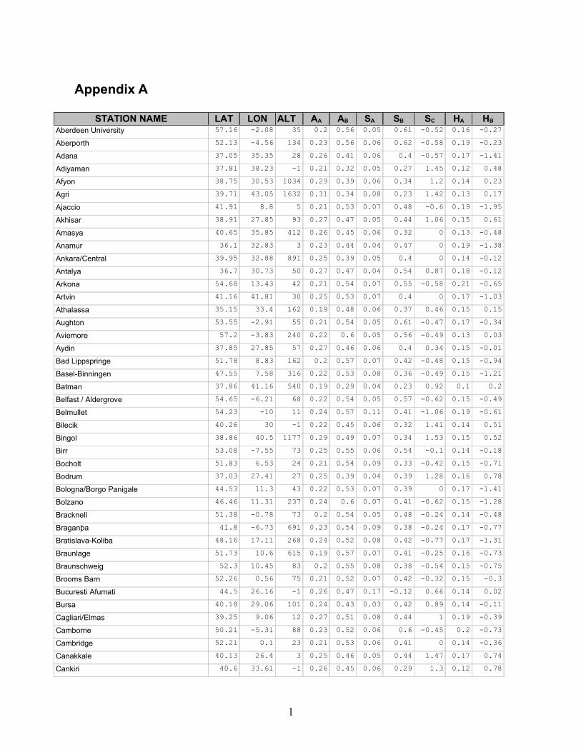
Appendix A

STATION NAME LAT LON ALT AA AB SA SB SC HA HB

Aberdeen University 57.16 -2.08 35 0.2 0.56 0.05 0.61 -0.52 0.16 -0.27

Aberporth 52.13 -4.56 134 0.23 0.56 0.06 0.62 -0.58 0.19 -0.23

Adana 37.05 35.35 28 0.26 0.41 0.06 0.4 -0.57 0.17 -1.41

Adiyaman 37.81 38.23 -1 0.21 0.32 0.05 0.27 1.45 0.12 0.48

Afyon 38.75 30.53 1034 0.29 0.39 0.06 0.34 1.2 0.14 0.23

Agri 39.71 43.05 1632 0.31 0.34 0.08 0.23 1.42 0.13 0.17

Ajaccio 41.91 8.8 5 0.21 0.53 0.07 0.48 -0.6 0.19 -1.95

Akhisar 38.91 27.85 93 0.27 0.47 0.05 0.44 1.06 0.15 0.61

Amasya 40.65 35.85 412 0.26 0.45 0.06 0.32 0 0.13 -0.48

Anamur 36.1 32.83 3 0.23 0.44 0.04 0.47 0 0.19 -1.38

Ankara/Central 39.95 32.88 891 0.25 0.39 0.05 0.4 0 0.14 -0.12

Antalya 36.7 30.73 50 0.27 0.47 0.04 0.54 0.87 0.18 -0.12

Arkona 54.68 13.43 42 0.21 0.54 0.07 0.55 -0.58 0.21 -0.65

Artvin 41.16 41.81 30 0.25 0.53 0.07 0.4 0 0.17 -1.03

Athalassa 35.15 33.4 162 0.19 0.48 0.06 0.37 0.46 0.15 0.15

Aughton 53.55 -2.91 55 0.21 0.54 0.05 0.61 -0.47 0.17 -0.34

Aviemore 57.2 -3.83 240 0.22 0.6 0.05 0.56 -0.49 0.13 0.03

Aydin 37.85 27.85 57 0.27 0.46 0.06 0.4 0.34 0.15 -0.01

Bad Lippspringe 51.78 8.83 162 0.2 0.57 0.07 0.42 -0.48 0.15 -0.94

Basel-Binningen 47.55 7.58 316 0.22 0.53 0.08 0.36 -0.49 0.15 -1.21

Batman 37.86 41.16 540 0.19 0.29 0.04 0.23 0.92 0.1 0.2

Belfast / Aldergrove 54.65 -6.21 68 0.22 0.54 0.05 0.57 -0.62 0.15 -0.49

Belmullet 54.23 -10 11 0.24 0.57 0.11 0.41 -1.06 0.19 -0.61

Bilecik 40.26 30 -1 0.22 0.45 0.06 0.32 1.41 0.14 0.51

Bingol 38.86 40.5 1177 0.29 0.49 0.07 0.34 1.53 0.15 0.52

Birr 53.08 -7.55 73 0.25 0.55 0.06 0.54 -0.1 0.14 -0.18

Bocholt 51.83 6.53 24 0.21 0.54 0.09 0.33 -0.42 0.15 -0.71

Bodrum 37.03 27.41 27 0.25 0.39 0.04 0.39 1.28 0.16 0.78

Bologna/Borgo Panigale 44.53 11.3 43 0.22 0.53 0.07 0.39 0 0.17 -1.41

Bolzano 46.46 11.31 237 0.24 0.6 0.07 0.41 -0.62 0.15 -1.28

Bracknell 51.38 -0.78 73 0.2 0.54 0.05 0.48 -0.24 0.14 -0.48

Braganþa 41.8 -6.73 691 0.23 0.54 0.09 0.38 -0.24 0.17 -0.77

Bratislava-Koliba 48.16 17.11 268 0.24 0.52 0.08 0.42 -0.77 0.17 -1.31

Braunlage 51.73 10.6 615 0.19 0.57 0.07 0.41 -0.25 0.16 -0.73

Braunschweig 52.3 10.45 83 0.2 0.55 0.08 0.38 -0.54 0.15 -0.75

Brooms Barn 52.26 0.56 75 0.21 0.52 0.07 0.42 -0.32 0.15 -0.3

Bucuresti Afumati 44.5 26.16 -1 0.26 0.47 0.17 -0.12 0.66 0.14 0.02

Bursa 40.18 29.06 101 0.24 0.43 0.03 0.42 0.89 0.14 -0.11

Cagliari/Elmas 39.25 9.06 12 0.27 0.51 0.08 0.44 1 0.19 -0.39

Camborne 50.21 -5.31 88 0.23 0.52 0.06 0.6 -0.45 0.2 -0.73

Cambridge 52.21 0.1 23 0.21 0.53 0.06 0.41 0 0.14 -0.36

Canakkale 40.13 26.4 3 0.25 0.46 0.05 0.44 1.47 0.17 0.74

Cankiri 40.6 33.61 -1 0.26 0.45 0.06 0.29 1.3 0.12 0.78

1

Cardington 52.1 -0.41 28 0.22 0.54 0.06 0.47 0 0.13 -0.27

Castelo Branco 39.83 -7.48 386 0.23 0.56 0.08 0.42 0.49 0.18 -0.11

Cawood 53.83 -1.13 6 0.21 0.54 0.04 0.53 -0.32 0.13 -0.08

Chemnitz 50.8 12.86 418 0.21 0.6 0.06 0.5 -0.28 0.17 -0.71

Churanov 49.06 13.61 1122 0.18 0.57 0.06 0.42 0 0.15 -0.7

Chur-Ems 46.86 9.53 555 0.25 0.54 0.07 0.37 0 0.14 -0.2

Clones 54.18 -7.23 89 0.24 0.54 0.12 0.31 -0.61 0.17 -0.58

Coburg 50.26 10.95 357 0.2 0.56 0.09 0.29 -0.42 0.15 -0.94

Coimbra 40.2 -8.41 141 0.25 0.51 0.09 0.37 0.27 0.17 -0.56

Corum 40.55 34.96 776 0.26 0.43 0.06 0.32 1.44 0.12 0.43

Crawley 51.08 -0.21 144 0.19 0.54 0.05 0.5 -0.68 0.15 -0.85

Crotone 39 17.06 171 0.3 0.48 0.06 0.46 1.4 0.18 0.44

Dalaman 36.7 28.78 7 0.25 0.45 0.05 0.4 1.33 0.16 0.15

De Bilt 52.1 5.18 38 0.21 0.54 0.06 0.41 -0.35 0.15 -0.77

De Kooy 52.91 4.78 2 0.23 0.54 0.07 0.53 -0.16 0.19 -0.41

Deir Ezzor 35.26 40.16 215 0.3 0.44 0.05 0.46 0 0.17 -0.67

Denizli 37.76 29.08 428 0.21 0.33 0.06 0.27 0 0.13 -0.7

Dikili 39.05 26.86 3 0.23 0.39 0.04 0.45 0 0.16 -0.63

Diyarbakir 37.88 40.18 686 0.28 0.45 0.04 0.45 1.37 0.15 0.06

Dresden-Klotzsche 51.13 13.75 230 0.21 0.54 0.06 0.46 -0.19 0.15 -0.52

Dublin Airport 53.43 -6.23 71 0.23 0.51 0.06 0.57 -0.49 0.15 -0.39

Dundee 56.45 -3.06 30 0.21 0.57 0.06 0.56 -0.61 0.16 -0.24

Dunstaffnage 56.46 -5.43 3 0.22 0.59 0.06 0.56 -0.25 0.17 -0.57

East Craigs 55.95 -3.33 61 0.24 0.51 0.05 0.55 0.21 0.14 0.56

East Malling 51.28 0.45 37 0.2 0.54 0.07 0.44 -0.6 0.15 -0.63

Edirne 41.73 26.61 -1 0.19 0.33 0.04 0.28 0 0.1 -0.1

Edremit 39.61 27.03 -1 0.29 0.46 0.05 0.44 1.49 0.16 0.86

Eelde 53.13 6.58 2 0.22 0.54 0.05 0.45 -0.1 0.14 -0.52

Eindhoven 51.45 5.41 23 0.21 0.54 0.06 0.41 -0.45 0.14 -0.82

Elazig 38.6 39.28 902 0.29 0.36 0.05 0.35 1.75 0.13 0.94

Erzincan 39.73 39.5 1156 0.28 0.41 0.09 0.21 0 0.13 -0.4

Erzurum 39.91 41.26 1756 0.39 0.31 0.02 0.42 4.76 0.12 3.57

Eskdalemuir 55.31 -3.2 242 0.19 0.59 0.04 0.55 -0.24 0.13 -0.36

Eskisehir 39.78 30.56 785 0.26 0.34 0.03 0.38 1.92 0.11 1.16

Evora 38.56 -7.9 309 0.27 0.52 0.08 0.45 0.6 0.17 0.95

Fahy 47.43 6.95 596 0.22 0.52 0.07 0.42 -0.17 0.16 -1.17

Faro/Aeroporto 37.01 -7.96 8 0.3 0.45 0.1 0.37 0.9 0.2 0.06

Fichtelberg 50.43 12.95 1219 0.17 0.61 0.05 0.54 0.45 0.17 -0.71

Finike 36.3 30.15 3 0.24 0.39 0.03 0.44 0.59 0.15 0.37

Finningley 53.48 -1 10 0.21 0.53 0.05 0.5 -0.36 0.14 -0.25

Foggia Amendola 41.43 15.55 57 0.27 0.52 0.08 0.41 0.55 0.17 -0.32

Freiburg 48 7.85 308 0.19 0.57 0.09 0.39 -0.74 0.17 -1.56

Froson Sol 63.2 14.5 -1 0.25 0.56 0.04 0.63 0 0.16 0.12

Garston 51.7 -0.38 77 0.19 0.54 0.06 0.45 -0.48 0.14 -0.76

Geisenheim 49.98 7.95 131 0.2 0.55 0.08 0.37 -0.6 0.15 -1.17

Gela 37.08 14.21 22 0.35 0.43 0.05 0.58 0.69 0.25 -0.11

Gemerek 39.18 36.05 1171 0.36 0.43 0.03 0.45 3.35 0.13 3

2

Geneve-Cointrin 46.25 6.13 420 0.25 0.5 0.06 0.45 -0.25 0.15 -1.09

Genova/Sestri 44.41 8.85 2 0.22 0.55 0.08 0.5 -0.38 0.22 -1.93

Giessen 50.58 8.7 201 0.19 0.58 0.09 0.32 -0.5 0.15 -0.88

Glarus 47.03 9.06 515 0.21 0.63 0.07 0.38 -0.5 0.14 -1.02

Gogerddan 52.43 -4.01 40 0.21 0.56 0.06 0.55 -0.69 0.16 -0.48

Goteborg Sol 57.7 12 5 0.21 0.56 0.02 0.68 -0.63 0.16 -0.33

Granada - Aeropuerto 37.18 -3.78 569 0.3 0.44 0.08 0.28 1.86 0.14 0.95

Great Horkesley 51.95 0.88 50 0.23 0.5 0.07 0.42 -0.34 0.15 -0.35

Grendon Underwood 51.9 -1.01 70 0.21 0.54 0.05 0.47 0 0.13 -0.29

Guettingen 47.6 9.28 440 0.22 0.55 0.08 0.35 -0.12 0.16 -1.4

Gumushane 40.45 39.45 1219 0.32 0.42 0.08 0.32 0.89 0.15 0.33

Hakkari 37.56 43.76 1720 0.32 0.32 0.05 0.36 2.6 0.15 1.84

Hamburg-Sasel 53.65 10.11 49 0.19 0.55 0.07 0.44 -0.72 0.15 -0.91

Hazelrigg 54.01 -2.75 95 0.22 0.57 0.06 0.56 -0.84 0.17 -0.64

Heiligendamm 54.15 11.85 21 0.21 0.55 0.05 0.59 -0.17 0.18 -0.17

Helsinki-Vantaa 60.31 24.96 53 0.21 0.57 0.04 0.56 -0.14 0.16 -0.52

Hemsby 52.68 1.68 13 0.22 0.52 0.05 0.57 -0.35 0.17 -0.02

Hinterrhein 46.51 9.18 1611 0.29 0.57 0.1 0.3 0 0.16 -0.61

Hohenpeissenberg 47.8 11.01 990 0.2 0.6 0.05 0.55 0.43 0.17 0.04

Hradec Kralove 50.18 15.83 -1 0.2 0.57 0.08 0.36 -0.59 0.15 -1.15

Hurbanovo 47.87 18.19 115 0.26 0.49 0.08 0.37 -0.95 0.16 -1.47

Interlaken 46.66 7.86 580 0.22 0.58 0.08 0.36 -0.48 0.15 -1.23

Iskenderun 36.58 36.16 3 0.21 0.37 0.05 0.43 -0.67 0.19 -1.58

Isparta 37.75 30.55 997 0.23 0.29 0.02 0.37 2.04 0.1 1.91

Istanbul/Goztepe 40.96 29.08 33 0.24 0.45 0.05 0.44 0 0.19 -1.09

Izra' 32.85 36.23 570 0.24 0.53 0.07 0.45 -1.47 0.17 -1.56

Jableh 35.37 35.95 36 0.26 0.36 0.04 0.43 0.8 0.16 -0.25

Jersey 49.18 -2.18 85 0.22 0.55 0.06 0.58 -0.47 0.21 -0.74

Jokioinen 60.81 23.5 104 0.21 0.58 0.05 0.53 0.2 0.15 -0.16

Jyvaskyla 62.4 25.68 141 0.21 0.57 0.03 0.6 0.21 0.14 -0.15

Kahramanmaras 37.6 36.93 549 0.24 0.52 0.05 0.46 0 0.18 -1.48

Karlstad Sol 59.36 13.46 46 0.23 0.54 0.04 0.6 -0.16 0.16 -0.44

Kassel 51.3 9.45 237 0.21 0.55 0.08 0.39 -0.52 0.15 -0.85

Kastamonu 41.36 33.76 799 0.22 0.36 0.05 0.27 0.8 0.11 0.31

Kayseri/Erkilet 38.78 35.48 1053 0.26 0.29 0.03 0.34 1.96 0.1 1.07

Kharabo 33.5 36.45 620 0.31 0.32 0.03 0.36 2.5 0.1 2.45

Kilkenny 52.66 -7.26 66 0.26 0.56 0.06 0.58 -0.35 0.15 -0.36

Kirikkale 39.88 33.53 -1 0.25 0.43 0.06 0.37 0.82 0.15 -0.13

Kirsehir 39.13 34.16 995 0.33 0.32 0.06 0.32 2.27 0.14 1.27

Kiruna Sol 67.83 20.43 -1 0.25 0.57 0.04 0.57 0.41 0.14 0.33

Klagenfurt-Flughafen 46.65 14.33 448 0.22 0.53 0.07 0.38 -0.24 0.14 -0.72

Klodzko 54.43 16.61 356 0.21 0.47 0.04 0.47 0 0.13 -0.06

Kocelovice 49.46 13.83 519 0.2 0.54 0.08 0.38 -0.41 0.15 -0.82

Kolobzreg 54.18 15.58 3 0.26 0.52 0.04 0.68 0 0.18 -0.26

Konstanz 47.68 9.18 450 0.2 0.57 0.09 0.35 -0.59 0.16 -1.4

Konya 37.96 32.55 1032 0.32 0.42 0.03 0.52 1.79 0.15 0.97

Konya/Eregli 37.5 34.06 1044 0.31 0.38 0.05 0.35 1.87 0.14 1.02

3

Kramolin-Kosetice 49.56 15.06 534 0.2 0.53 0.08 0.35 -0.22 0.15 -0.77

Kucharovice 48.88 16.08 334 0.2 0.53 0.07 0.37 -0.49 0.15 -0.85

Kusadasi 37.91 27.3 -1 0.29 0.38 0.06 0.37 1.6 0.17 0.59

La Rochelle 46.15 -1.15 4 0.24 0.5 0.08 0.46 0.57 0.19 0.03

Leconfield 53.86 -0.43 6 0.24 0.45 0.06 0.46 0 0.14 -0.06

Lerwick 60.13 -1.18 82 0.22 0.61 0.07 0.6 -0.55 0.19 -0.55

Lindenberg 52.21 14.11 98 0.19 0.52 0.06 0.41 -0.38 0.15 -0.6

Lisboa/Geof 38.71 -9.15 77 0.24 0.52 0.13 0.31 0.6 0.21 -0.63

List/Sylt 55.01 8.41 33 0.22 0.56 0.07 0.54 -0.34 0.21 -0.51

Ljubljana - Bezigrad 46.06 14.51 299 0.21 0.63 0.09 0.39 -0.7 0.17 -1.83

Logrono - Agoncillo 42.63 -2.4 364 0.22 0.55 0.09 0.32 0 0.15 -0.86

London Weather Centre 51.51 -0.11 77 0.18 0.53 0.06 0.48 -0.62 0.16 -0.61

Long Ashton 51.43 -2.66 51 0.2 0.55 0.05 0.54 -0.55 0.15 -0.53

Lugano 46 8.96 273 0.19 0.54 0.07 0.45 -0.48 0.17 -0.95

Luka 49.05 16.95 513 0.2 0.54 0.08 0.38 -0.4 0.16 -0.89

Lulea Sol 65.55 22.13 17 0.24 0.54 0.03 0.65 -0.1 0.17 -0.32

Lund Sol 55.71 13.21 73 0.22 0.55 0.07 0.44 -0.12 0.17 -0.64

Luzern 47.03 8.3 456 0.22 0.55 0.07 0.36 0.14 0.15 -1.39

Malatya/Erhac 38.43 38.08 862 0.29 0.37 0.08 0.28 1.78 0.15 0.84

Mannheim 49.51 8.55 106 0.19 0.55 0.08 0.38 -0.83 0.15 -1.35

Marmaris 36.83 28.26 3 0.21 0.46 0.05 0.43 0 0.18 -1.25

Mersin 36.81 34.6 3 0.27 0.47 0.06 0.54 -0.73 0.25 -3.11

Messina 38.2 15.55 54 0.25 0.55 0.09 0.5 0.49 0.24 -0.81

Milano / Linate 45.43 9.28 120 0.23 0.55 0.08 0.4 -0.68 0.18 -1.93

Milhostov 48.66 21.72 105 0.24 0.44 0.06 0.34 0 0.14 -0.76

Missilmieh 36.32 37.22 415 0.24 0.45 0.05 0.45 0 0.16 -1.03

Mugla 37.2 28.35 646 0.19 0.47 0.01 0.48 0.65 0.13 0.13

Murcia 37.98 -1.11 62 0.27 0.48 0.11 0.24 -0.21 0.16 -0.85

Mus 38.73 41.51 1320 0.29 0.34 0.04 0.34 2.97 0.13 1.11

Napoli Capodichino 40.85 14.3 88 0.26 0.5 0.08 0.43 -0.24 0.18 -1.79

Neubrandenburg 53.55 13.2 83 0.2 0.55 0.09 0.36 -0.43 0.16 -0.68

Neuchatel 47 6.95 485 0.22 0.55 0.08 0.39 0 0.17 -1.3

Nice 43.65 7.2 4 0.21 0.53 0.09 0.5 -1.45 0.25 -3.08

Nigde 37.96 34.68 1208 0.39 0.41 0.06 0.42 3.12 0.17 1.94

Norderney 53.71 7.15 29 0.22 0.55 0.06 0.58 -0.24 0.21 -0.05

Norrkoping Sol 58.58 16.15 -1 0.22 0.55 0.04 0.55 -0.27 0.15 -0.42

Nuernberg 49.5 11.08 312 0.19 0.54 0.07 0.4 -0.46 0.15 -0.98

Olbia/Costa Smeralda 40.9 9.51 12 0.24 0.54 0.07 0.51 -0.52 0.18 -1.2

Ordu 41.06 37.53 -1 0.21 0.57 0.08 0.38 -0.66 0.19 -2.92

Osnabrueck 52.25 8.05 104 0.2 0.56 0.09 0.32 -0.45 0.15 -0.81

Ostrava Poruba 49.81 19.15 -1 0.17 0.57 0.06 0.38 -0.46 0.13 -0.89

Oviedo 43.35 -5.86 348 0.24 0.57 0.1 0.38 -0.51 0.17 -1

Palma de Mallorca 39.55 2.61 8 0.25 0.48 0.07 0.42 -0.31 0.17 -1.13

Payerne 46.81 6.95 490 0.23 0.53 0.08 0.4 -0.13 0.15 -1.07

Penhas Douradas 40.41 -7.55 1380 0.25 0.55 0.08 0.48 1.28 0.21 -0.04

Perpignan 42.73 2.86 42 0.21 0.53 0.07 0.5 -0.19 0.18 -0.76

Pescara 42.43 14.2 16 0.26 0.56 0.08 0.45 0 0.19 -1.96

4

Piotta 46.51 8.68 1007 0.2 0.62 0.08 0.39 -1.3 0.16 -1.58

Pisa/S. Giusto 43.68 10.38 11 0.25 0.55 0.08 0.44 -0.44 0.18 -1.79

Porto/Serra do Pilar 41.13 -8.6 93 0.25 0.53 0.1 0.39 0 0.2 -1.69

Potsdam (SMR) 52.36 13.08 107 0.19 0.54 0.09 0.33 -0.83 0.15 -0.97

Praha 2 50.06 14.41 -1 0.19 0.52 0.07 0.37 -0.61 0.14 -0.9

Pully 46.51 6.66 461 0.25 0.51 0.09 0.38 0 0.18 -0.84

Raqqa 35.9 38.98 246 0.26 0.45 0.06 0.39 0.55 0.16 -0.61

Reims 49.3 4.03 91 0.21 0.53 0.08 0.38 -0.15 0.15 -0.6

Rennes 48.06 -1.71 37 0.22 0.51 0.08 0.41 -0.14 0.16 -0.57

Reykjavik 64.13 -21.9 50 0.29 0.68 0.05 0.7 -0.09 0.19 -0.26

Rize 41.01 40.46 -1 0.2 0.55 0.05 0.49 -0.91 0.19 -3.03

Robbia 46.35 10.06 1078 0.21 0.71 0.06 0.41 0 0.14 -0.2

Roma/Ciampino 41.78 12.58 137 0.28 0.51 0.09 0.39 0 0.18 -1.24

Rothamsted 51.8 -0.35 128 0.21 0.5 0.06 0.43 -0.45 0.14 -0.67

Rustington 50.81 -0.51 8 0.23 0.53 0.07 0.45 -0.33 0.16 -0.35

Saarbruecken/Ensheim 49.21 7.11 325 0.19 0.55 0.08 0.42 -0.79 0.16 -1.43

Sakarya 40.78 30.41 30 0.24 0.52 0.07 0.38 0.37 0.17 -1.17

Salamanca - Matacan 40.95 -5.5 802 0.26 0.47 0.08 0.31 1.22 0.14 0.83

Samsun 41.28 36.33 4 0.23 0.51 0.06 0.5 0 0.2 -1.94

Schaffhausen 47.68 8.61 437 0.23 0.56 0.07 0.4 -0.55 0.16 -1.43

Schleswig 54.53 9.55 59 0.2 0.55 0.09 0.38 -0.35 0.16 -0.6

Scuol 46.8 10.28 1298 0.28 0.55 0.08 0.35 0.55 0.14 0.56

Seehausen 52.9 11.73 21 0.21 0.56 0.08 0.36 -0.35 0.15 -0.63

Siirt 37.93 42 895 0.25 0.38 0.06 0.3 1.81 0.15 0.46

Silifke 36.36 33.93 15 0.26 0.43 0.02 0.51 1.1 0.17 0.76

Silsoe 52.01 -0.41 59 0.22 0.53 0.06 0.46 0 0.14 -0.15

Sinop 42.03 35.16 32 0.23 0.46 0.07 0.37 0.6 0.2 -1.31

Sion 46.21 7.33 482 0.26 0.51 0.08 0.38 -0.6 0.15 -0.81

Sivas 39.75 37.01 1285 0.25 0.34 0.04 0.36 0.76 0.13 -0.03

Sodankyla 67.36 26.65 179 0.23 0.56 0.04 0.59 0.44 0.14 0.03

Stockholm Sol 59.35 18.06 -1 0.22 0.54 0.06 0.47 0 0.17 -0.22

Stornoway 58.21 -6.31 9 0.22 0.58 0.04 0.64 -0.53 0.17 -0.37

Strasbourg 48.55 7.63 150 0.21 0.54 0.07 0.42 -0.32 0.15 -1.05

Sunderland Polytechnic 54.9 -1.38 56 0.21 0.57 0.07 0.54 -0.44 0.17 -0.16

Sutton Bonington 52.83 -1.25 48 0.2 0.53 0.05 0.46 -0.2 0.13 -0.22

Svratouch 49.73 16.03 735 0.19 0.55 0.08 0.38 0 0.16 -0.63

Tatvan 38.51 42.26 1664 0.29 0.36 0.07 0.27 0.93 0.14 0.11

Tekirdag 40.98 27.48 4 0.21 0.48 0.05 0.38 0.34 0.17 -1.22

Toravere 58.26 26.46 70 0.21 0.54 0.18 -0.19 0.75 0.15 -0.17

Torino / Caselle 45.21 7.65 308 0.25 0.55 0.08 0.39 -0.17 0.18 -1.55

Trabzon 41 39.71 35 0.23 0.46 0.04 0.47 -0.31 0.18 -1.63

Trapani/Birgi 37.91 12.5 14 0.32 0.46 0.06 0.54 1.14 0.19 0.81

Trier-Petrisberg 49.75 6.66 278 0.2 0.57 0.08 0.38 -0.71 0.15 -1.1

Trieste 45.65 13.75 12 0.22 0.58 0.07 0.5 0.29 0.2 -0.19

Tusimice 50.38 13.33 322 0.2 0.55 0.06 0.38 -0.41 0.14 -0.88

Twenthe 52.26 6.9 35 0.21 0.53 0.07 0.41 -0.55 0.14 -0.78

Umea Sol 63.83 20.25 -1 0.23 0.55 0.04 0.57 0 0.16 -0.28

5

Usak 38.66 29.41 919 0.26 0.43 0.05 0.38 0.71 0.14 0.41

Usti Nad Labem 50.68 14.03 377 0.2 0.55 0.07 0.39 -0.97 0.16 -1.46

Ustica 38.7 13.18 259 0.29 0.5 0.05 0.57 1.96 0.23 2

Utsjoki - Kevo 69.75 27.03 107 0.24 0.56 0.04 0.56 0.71 0.13 0.49

Vaduz (Liechtenstein) 47.13 9.51 460 0.21 0.6 0.07 0.38 -0.14 0.15 -1.1

Valentia Observatory 51.93 -10.25 11 0.24 0.59 0.07 0.59 -0.56 0.18 -1.04

Van 38.45 43.31 1667 0.31 0.42 0.07 0.4 2.36 0.18 0.95

Vaxjo Sol 56.93 14.73 182 0.22 0.55 0.05 0.5 -0.15 0.15 -0.48

Vigna di Valle 42.08 12.21 270 0.24 0.53 0.1 0.4 -0.14 0.19 -0.56

Visby Sol 57.66 18.35 28 0.23 0.53 0.03 0.67 -0.12 0.18 0.02

Visp 46.3 7.85 640 0.26 0.52 0.1 0.3 -1.61 0.16 -1.58

Wallingford 51.6 -1.16 49 0.2 0.54 0.05 0.47 -0.45 0.13 -0.57

Wareham 50.66 -2.18 10 0.24 0.49 0.06 0.5 0 0.16 -0.16

Weihenstephan 48.4 11.7 472 0.22 0.55 0.08 0.38 0 0.15 -0.82

Weimar 50.98 11.31 257 0.21 0.51 0.08 0.32 -0.33 0.14 -0.74

Weissenburg 49.01 10.96 428 0.2 0.55 0.08 0.37 -0.36 0.15 -0.87

Wellesbourne 52.2 -1.6 48 0.24 0.52 0.07 0.44 0 0.14 0.02

Wuerzburg 49.76 9.96 275 0.23 0.54 0.08 0.37 -0.41 0.15 -0.86

Wye 51.18 0.95 59 0.23 0.51 0.07 0.46 -0.7 0.16 -0.84

Wynau 47.25 7.78 422 0.23 0.54 0.08 0.34 -0.31 0.15 -1.47

Yozgat 39.83 34.81 1298 0.27 0.37 0.07 0.27 1.82 0.14 0.69

Zagreb/Gric 45.81 15.98 157 0.21 0.56 0.1 0.31 -0.67 0.16 -1.79

Zinnwald-Georgenfeld 50.73 13.75 877 0.21 0.6 0.07 0.46 0.49 0.17 -0.04

Zuid Limburg 50.91 5.78 2 0.21 0.54 0.06 0.41 -0.33 0.15 -0.83

Zurich-(Town/Ville) 47.38 8.56 556 0.21 0.57 0.06 0.46 -0.43 0.16 -1.41

6