technical note 2011/02 - waterconnect.sa.gov.au

TECHNICAL NOTE 2011/02 Department for Water

© Government of South Australia, through the Department for Water 2011

This work is Copyright. Apart from any use permitted under the Copyright Act 1968 (Cwlth), no part may be

reproduced by any process without prior written permission obtained from the Department for Water. Requests and

enquiries concerning reproduction and rights should be directed to the Chief Executive, Department for Water, GPO

Box 2834, Adelaide SA 5001.

Disclaimer

The Department for Water and its employees do not warrant or make any representation regarding the use, or results

of the use, of the information contained herein as regards to its correctness, accuracy, reliability, currency or

otherwise. The Department for Water and its employees expressly disclaims all liability or responsibility to any person

using the information or advice. Information contained in this document is correct at the time of writing. Information

contained in this document is correct at the time of writing.

ISBN 978-1-921923-02-9

Preferred way to cite this publication

Alcorn M. R., 2011, Hydrological Modelling of the Eastern Mount Lofty Ranges: Demand and Low Flow Bypass

scenarios, DFW Technical Note 2011/02, Department for Water, Adelaide

Department for Water

Science, Monitoring and Information Division

25 Grenfell Street, Adelaide

GPO Box 2834, Adelaide SA 5001

Telephone National (08) 8463 6946

International +61 8 8463 6946

Fax National (08) 8463 6999

International +61 8 8463 6999

Website www.waterforgood.sa.gov.au

Download this document at:

http://www.waterconnect.sa.gov.au/TechnicalPublications/Pages/default.aspx

Hydrological Modelling of the Eastern Mount Lofty Ranges: Demand and Low Flow Bypass scenarios

Mark R Alcorn

February 2011

Technical note 2011/02 1


SUMMARY

The Science, Monitoring and Information (SMI) Division within the Department for Water (DFW) was

engaged by the SA Murray-Darling Basin Natural Resources Management Board (SAMDBNRM) to

undertake surface water demand modelling of the Eastern Mount Lofty Ranges (EMLR) Prescribed

Water Resources Area (PWRA) for the scenarios where Low-Flow Bypass (LFB) occurs at:

All irrigation dams; and

All dams with a cease-to-flow storage volume of 5 megalitres (ML) or greater

This report also investigates the impact of various demand scenarios on the daily stream flow

regime, as well as the effects on the annual water balance of the modelled catchments. It also

details the modelling assumptions and methods employed to pass low flows around dams, vary

demand from irrigation dams and set threshold flow rates for watercourse extractions. The outputs

from this report, daily time step stream flow estimates at 63 test sites, have been delivered to the

SAMDBNRMB. These outputs are intended to be analysed by the SAMDBNRMB with regard to

meeting the environmental water requirements (EWR) metrics and targets through the adoption of

any, or a combination of the scenarios presented. The outcome of the analysis is likely that the

SAMDBNRMB will be able to establish Consumptive Use Limits (CUL) and Threshold Flow Rates (TFR)

where flows will be required to be bypassed.

This report should be read in conjunction with the following, which have also been delivered to the

SAMDBNRMB as part of this work:

Environmental Water Requirements (EWR) spreadsheets (EWR_Scenarios2010.xlsm); and

Data folders containing individual stream flow records for each EWR result spreadsheet for

testing locations.

The results of this modelling indicate that providing low flows to the catchments downstream of

selected irrigation and large stock and domestic dams would provide an overall increase in mean

annual end of system flows of around 2%. There appears to be minimal difference in the total

volume of flows (at the mean annual streamflow scale) delivered by either the “Irrigation Dam only”

scenario or the scenario with “additional LFB on large (>= 5 ML) stock and domestic dams”.

However, analysis of the daily flow regime suggest that there will be appreciable benefits to the low-

flow regime, particularly during the low flow and transition seasons of January through to June, and

in particular for the scenario of “LFB on large stock and domestic dams and all irrigation dams”.


Contents

SUMMARY ............................................................................................................................................. 2

INTRODUCTION ..................................................................................................................................... 6

AIM. ........................................................................................................................................................................ 6

SCOPE. ........................................................................................................................................................................ 6

BACKGROUND ............................................................................................................................................................... 6

LOW FLOW RELEASE RATES .................................................................................................................... 8

UNIT THRESHOLD FLOW RATES .................................................................................................................................... 8

SCENARIO MODELLING .......................................................................................................................... 9

SCENARIO DESCRIPTIONS ............................................................................................................................................. 9

SCENARIO 1: NO FARM DAMS OR WATERCOURSE EXTRACTIONS .......................................................... 11

SCENARIO 2: CURRENT ESTIMATE OF DEMAND – WITHOUT LOW-FLOW RELEASES ................................ 11

WATER USE DATA ....................................................................................................................................................... 11

FARM DAMS DATA ...................................................................................................................................................... 11

Summary ..................................................................................................................................................... 12

WATER USE FROM FARM DAMS ................................................................................................................................. 13

Internal Annual Use Fraction ...................................................................................................................... 13

Definition of monthly usage distribution patterns ..................................................................................... 14

NET EVAPORATION FROM DAMS ............................................................................................................................... 16

SCENARIO 3, SCENARIO 4 AND SCENARIO 5 .......................................................................................... 19

DEMAND FROM FARM DAMS ..................................................................................................................................... 19

Variation of Usage from Lumped Dam Nodes where there is a combination of Licensed Irrigation Dams

and Non-licensed Stock and Domestic dams .............................................................................................. 20

VARIATION OF DEMAND FROM WATERCOURSE EXTRACTIONS AND LOW FLOW BYPASS

CONDITIONS. ............................................................................................................................................................... 21

Watercourse extraction estimates: Catchment Scale ................................................................................. 22

Selection of sub-catchments for low flow releases .................................................................................... 22

Description of programs and data required to process inputs and outputs ............................................... 22

RESULTS .............................................................................................................................................. 34

FARM DAMS ................................................................................................................................................................ 34

MODEL SUB-CATCHMENTS ......................................................................................................................................... 34

WATER USE ESTIMATES FOR DEMAND SCENARIOS .................................................................................................... 34

CATCHMENT WATER BALANCES ................................................................................................................................. 35

EFFECT OF LFB AND DEMAND SCENARIOS ON DAILY FLOW ....................................................................................... 37

Site B18 Results ........................................................................................................................................... 38

Site F15 Results ........................................................................................................................................... 40

REFERENCES ........................................................................................................................................ 42


Table of Figures

Figure 1. Unit Threshold Flow rates For the EMLR ..................................................................................................... 8

Figure 2. EMLR Prescribed Area showing model Domains ....................................................................................... 10

Figure 3. Monthly Usage Distribution Patterns......................................................................................................... 15

Figure 4. Farm dam area-volume relationship at less than full supply level............................................................. 17

Figure 5. Range of dam volume exceedences ........................................................................................................... 18

Figure 6. Mean monthly storage volume of EMLR Farm Dams ................................................................................ 18

Figure 7. Watercourse Extraction Set-up WaterCRESS Model .................................................................................. 21

Figure 8. Angas River Testing Sites and LFB Selection Scenario 4 ............................................................................ 25

Figure 9. Bremer River Testing Sites and LFB Selection Scenario 4 .......................................................................... 26

Figure 10. Currency Creek Testing Sites and LFB Selection Scenario 4 ....................................................................... 27

Figure 11. Finniss River Testing Sites and LFB Selection Scenario 4 ........................................................................... 28

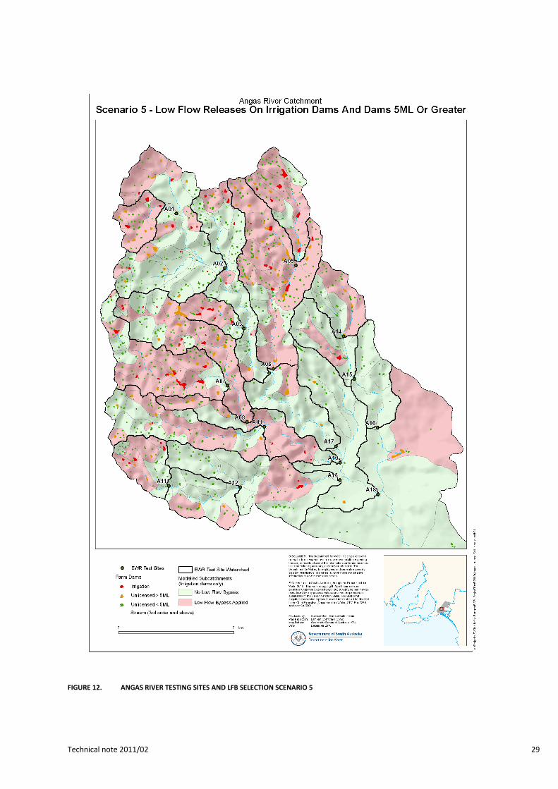
Figure 12. Angas River Testing Sites and LFB Selection Scenario 5 ............................................................................. 29

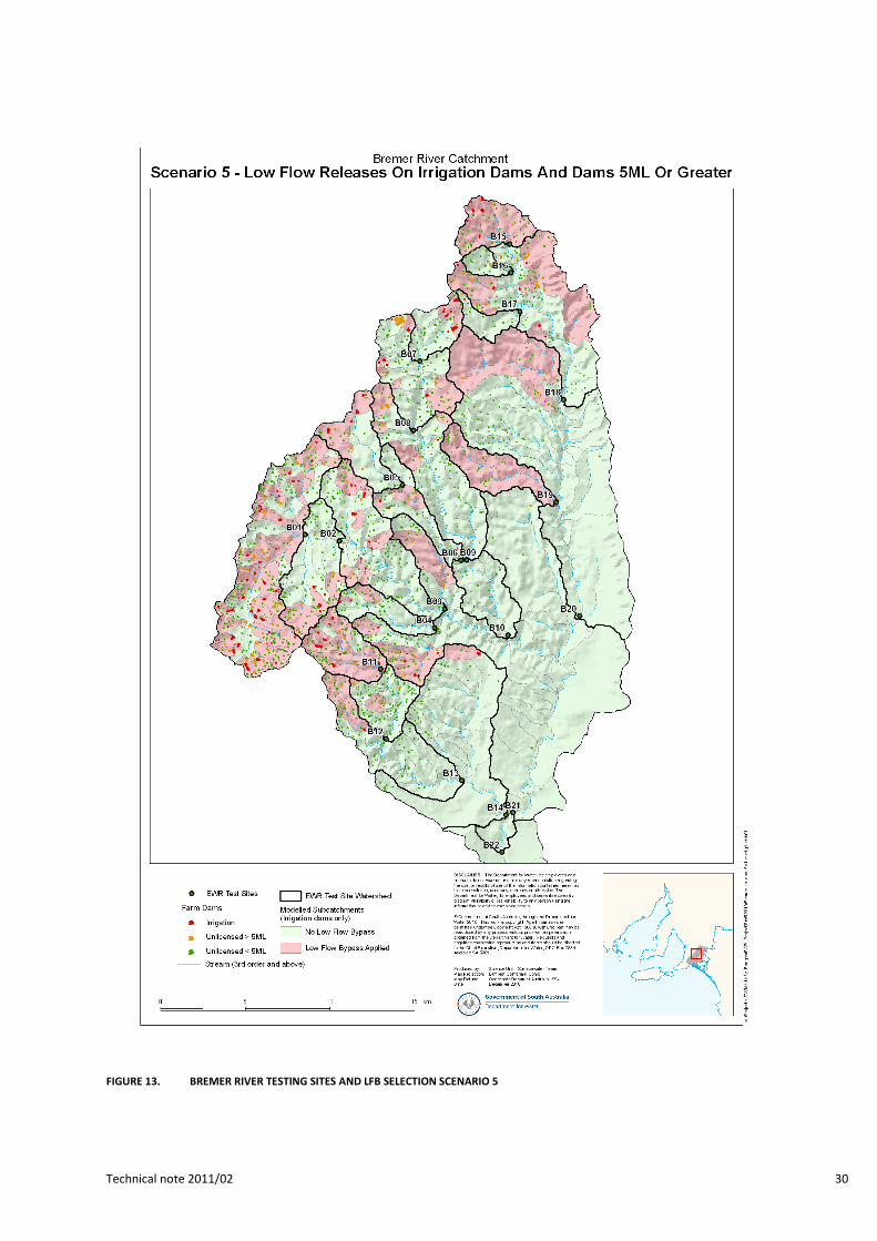
Figure 13. Bremer River Testing Sites and LFB Selection Scenario 5 .......................................................................... 30

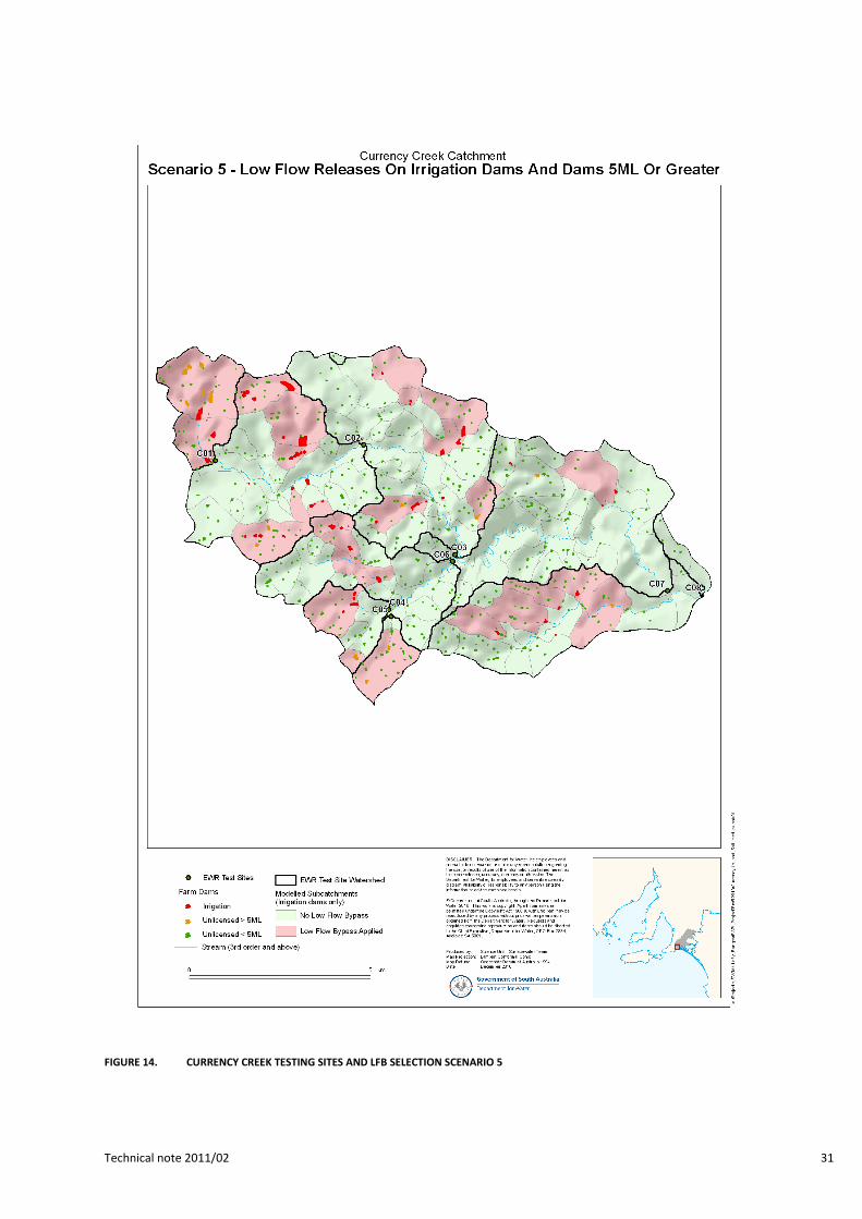
Figure 14. Currency Creek Testing Sites and LFB Selection Scenario 5 ....................................................................... 31

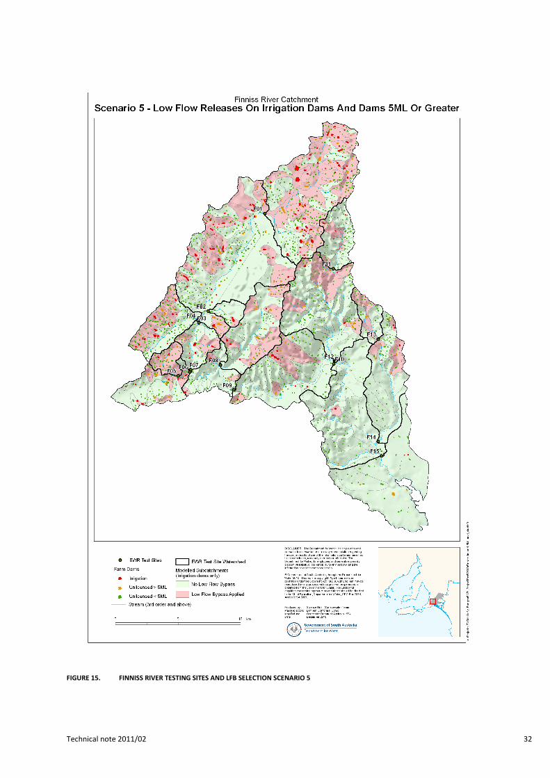
Figure 15. Finniss River Testing Sites and LFB Selection Scenario 5 ............................................................................ 32

Figure 16. Model Layout comparison of Scenarios 4 and 5 for ewr Site B18 in the Upper Bremer River .................. 38

Figure 17. Flow Duration Curves for EWR Site B18 in the Upper Bremer River .......................................................... 39

Figure 18. Model Layout comparison of Scenarios 4 and 5 for ewr Site F15 in the Lower Finniss River .................... 40

Figure 19. Flow Duration Curves for EWR Site F15 in the Lower FINNISS RIVER ........................................................ 41

Table of Tables

Table 1. Farm Dam Statistics for the EMLR .............................................................................................................. 12

Table 2. Farm Dam Statistics for the Five Modelled Catchments in the EMLR ........................................................ 12

Table 3. Usage patterns for Irrigation Proportion Ranges ...................................................................................... 14

Table 4. Evaporation details for selected farm dams .............................................................................................. 17

Table 5. Annual demand and flux estimates ............................................................................................................ 19

Table 6. November–April demand and flux estimates ............................................................................................ 19

Table 7. Example for a 50% Irrigation Proportion ................................................................................................... 20

Table 8. Catchment-Scale WaterCourse Demand Estimates ................................................................................... 22

Table 9. Sub-catchments Selected for low flow bypass ........................................................................................... 22

Table 10. List of Scripts to run EWR Scenario Analysis .............................................................................................. 23

Table 11. Model Sub-catchments Selected for LFB ................................................................................................... 34

Table 12. Water usage as percent of total Catchment Runoff for various Demand scenarios .................................. 35

Table 13. Angas River Catchment Water Balance ...................................................................................................... 36

Table 14. Bremer River Catchment Water Balance ................................................................................................... 36

Table 15. Currency Creek Catchment Water Balance ................................................................................................ 36

Table 16. Finniss River Catchment Water Balance .................................................................................................... 37

Table 17. EWR Site Details for B18 in the Upper Bremer River ................................................................................. 38

Table 18. Daily Flow Statistics for EWR Site B18 in the Upper Bremer River ............................................................ 39

Table 19. EWR Site Details for F15 in the Lower Finniss River ................................................................................... 40

Table 20. Daily Flow Statistics for EWR Site F15 in the Lower Finniss River .............................................................. 40


INTRODUCTION

AIM

The aim of this report is to summarise the work of the Science Monitoring and Information (SMI)

Division within the Department for Water (DFW) in undertaking surface water modelling of the

Eastern Mount Lofty Ranges (EMLR) Prescribed Surface Water Area (PSWA) for a range of water

usage and Low Flow Bypass scenarios.

The scenarios where Low Flow Bypass (LFB) occurs at: 1. All irrigation dams; and

2. All irrigation dam and all stock and domestic dams with a cease-to-flow storage volume of 5

megalitres (ML) or greater, and for a range of water demands from dams and watercourses.

This work was requested by the SA Murray-Darling Basin Natural Resources Management Board

(SAMDBNRMB), to provide input to the determination of Environmental Water Requirements (EWR)

for the EMLR.

SCOPE

The intended scope of this report is to document the techniques and assumptions used to model the

effect of low flow bypasses on farm dams, threshold flow rates on watercourse extractions and

varying levels of water demand from the existing network of surface water development. The

primary outcomes of this modelling are files containing modelled daily flow estimates for 63 testing

sites over 4 catchment models within the EMLR.

Additional outputs of this study are:

the automated generation of individual files describing the EWRs for each test site for each modelling

scenario

A collated spreadsheet containing summaries of all models and results for each site and scenario.

The daily hydrological models used in this study cover Bremer River (Alcorn, 2008), Angas River

(Savadamuthu, 2006), Finniss River (Savadamuthu, 2003) and Currency Creek (Alcorn, M., 2006).

BACKGROUND

This work forms a part of the ongoing work by the DFW to provide science support to the process of

Prescription in the Eastern Mount Lofty Ranges (EMLR) Prescribed Water Resources Area (PWRA).

This is the third in a series of hydrological reports for the EMLR, and provides a range of water use

and management options to the SAMDBNRMB, for the purpose of assessment of Environmental

Water Requirements (EWRs) and eventually the Environmental Water Provisions (EWPs).

The first of these reports (Alcorn et al, 2008) sets out the basic framework for calculating the

capacity of the surface water resource of the EMLR, with regard particularly to the impacts of farm

dams on streamflow. The second report (Alcorn, 2010), revisited the existing hydrological models,

updating farm dam data and climate data, and included the impact of existing watercourse

extractions. It also provided the framework for estimating the average impacts of plantation forestry

on the landscape as required through the Statewide Policy Framework (SA Government, 2009).

This report describes the scenario modelling requested by the SAMDBNRMB, and any changes made

to the models since the estimates reported in DFW (2010). The outputs from this study are the

modified daily time series at a series of test sites throughout the EMLR.


LOW FLOW RELEASE RATES

At the time of writing, it was likely that intended policy options for the EMLR Water Allocation Plan

(WAP) will include the installation of some form of low-flow bypass device on licensable farm dams,

and watercourse extractions, or the requirement to release low flows to the environment some

other way. This report investigates the effect of including those releases. For licensable farm dams in

the models flows are bypassed around the dam, and for watercourse extractions only water above

the Unit Threshold Flow Rate (UTFR) may be extracted.

UNIT THRESHOLD FLOW RATES

The Unit Threshold Flow Rate (UTFR) is defined as the rate of flow per square kilometre of

catchment at or below which water must not be diverted or collected by a dam, wall or other

structure, and is expressed in litres/second/km2. This rate was set to be equivalent to the rate of

daily flow that is exceeded or equalled for 20% of the flowing period of the catchment. It is

calculated by removing the zero flow days from the record and calculating the daily flow that is

exceeded 20% of the time.

As calculating this value is not possible at the location of each and every dam or every watercourse

extraction or diversion, a regional curve was constructed using streamflow data from all available

gauging stations in the Mount Lofty Ranges and the corresponding rainfall in the catchment. This

curve is shown in Figure 11 below. This allows a variable UTFR to be used for any location in the

catchment, to be defined based upon the rainfall upstream of the dam or watercourse extraction in

question.

The rationale for choosing this threshold was that it is approximately equivalent to the definition of

a “T1 Fresh”, in the Environmental Water Requirements flow metrics (Van Laarhoven and van der

Wielen, 2009), and is relatively simple to calculate from measured streamflow data.

The UTFR for a dam (or a watercourse extraction) can be calculated by taking the mean annual

rainfall upstream of the dam (or the watercourse) location and finding that point on the x-axis of the

chart below, and finding the corresponding UTFR on the y-axis. Multiply the UTFR by the catchment

area above the dam (or the watercourse extraction) to give the location specific Threshold Flow Rate

(TFR) in litres per second.

FIGURE 1. UNIT THRESHOLD FLOW RATES FOR THE EMLR

0

0.5

1

1.5

2

2.5

3

3.5

4

4.5

5

0 100 200 300 400 500 600 700 800 900 1000

Un

it T

hre

sho

ld F

low

Rat

e (

l/s/

km2 )

Mean Annual Rainfall (mm)

Unit Threshold Flow Rates (L/Sec/Km2)


For all modelled catchments in this study, the relationship is defined as:

Where:

UTFR = the unit threshold flow rate in units of L/s/km2

P = the area weighted mean annual rainfall for the sub-catchment

SCENARIO MODELLING

Scenario modelling of water use from farm dams and watercourse extractions was undertaken

considering the following assumptions and limitations:

Water use from farm dams identified as being for Stock and Domestic use remain fixed at an

estimated 30% of the maximum capacity of the dam. This was a major assumption of the modelling

and was bound by the absence of any management mechanisms relating to water use from this dam

category (McMurray, 2004).

Demand scenarios were modelled for both irrigation dams and watercourse diversions so that a

range of water consumption could be used to assess the impact on the flow regime and hence, on

Environmental Water Requirements (EWRs).

SCENARIO DESCRIPTIONS

The scenarios that were modelled were: 1. “No dams or watercourse extractions” scenario: Often termed the “natural’ or “predevelopment

flow”, this is the scenario against which all other scenarios are tested for EWRs.

2. “Current” or “Base” scenario: Includes current estimated use from farm dams and watercourse

extractions, but does not model the impacts of plantation forestry.

3. “Varied usage on irrigation dams – no low-flow releases” scenario: A variation of Scenario 2,

where all irrigation dams and watercourse extraction have the demand varied.

4. “Varied usage on irrigation dams – low flow releases on irrigation dams only” scenario: Similar to

Scenario 3, but with the requirement to bypass low flows around irrigation dams and past

watercourse extractions.

5. “Varied usage on irrigation dams – low flow releases on irrigation dams and dams with a capacity

of 5 ML or greater” scenario: As Scenario 4, with the addition of low flow releases past large

(>5 ML) Stock and Domestic dams.

Figure 2 shows the model domain for the four hydrological models used in this report, which include

the Angas River, the Bremer River, Currency Creek, and the Finniss River. These are the only

catchments in the EMLR Prescribed Water Resources Area (PWRA) that currently have daily rainfall-

runoff models suitable for the purpose of EWR modelling. Although a similar daily hydrological

model exists for the Tookayerta catchment (Savadamuthu, 2004), this was not included in the

determination of the EWR of the EMLR due to the different nature of this catchment compared with

other Mount Lofty Ranges catchments (VanLaarhoven, et al., 2009).


FIGURE 2. EMLR PRESCRIBED AREA SHOWING MODEL DOMAINS


SCENARIO 1: NO FARM DAMS OR WATERCOURSE EXTRACTIONS

The “No dams or watercourse extractions” scenario: Often termed the “natural’ or “predevelopment

flow”, this is the scenario against which all other scenarios are tested for EWRs.

This scenario is modelled by removing all farm dams and watercourse extractions from the model.

Note that modelled urban areas (Bremer and Angas models) are not removed as this modelling is

focussed only on the impact of farm dams and watercourse extractions.

SCENARIO 2: CURRENT ESTIMATE OF DEMAND – WITHOUT LOW-FLOW RELEASES

The current or “Base” Case scenario includes current estimated use from farm dams and

watercourse extractions, but does not model the impacts of plantation forestry. The results of this

scenario are not discussed directly, but are considered as part of the range of results reported in

Scenario 3, which encompass a broader range of demand estimates. Described in this section are the

assumptions around farm dam water usage and extractions from streams.

WATER USE DATA

Water use across the modelled catchments in the EMLR is currently represented in the hydrological

models by:

farm dam extractions,

watercourse diversions and extractions, and

flood irrigation.

FARM DAMS DATA

Farm dam water use is dominant in the highlands of the EMLR and is categorised within this report

as either: 1. Irrigation: A dam from which water is used to irrigate land for commercial purposes. As this type of

water use is controlled under the WAP, dam types in this category are also termed “licensed dams”.

The terms “Licensed dam(s)” and “irrigation dam(s)” are used interchangeably in this report.

2. Stock and Domestic: A dam from which water is taken to water stock or for domestic use. As this type

of water use is not proposed to be controlled by the draft WAP, dam types in this category are also

termed non-licensed dams. The terms “Stock and Domestic dam(s)” and “non-licensed dam(s)” are

used interchangeably in this report.

Data describing farm dams in the EMLR is based on a combination of previously captured data and

updated estimates of licensed dam capacities and locations. Licensed dam locations and cease to

spill capacities of those dams were provided to this analysis by DFW's Water Planning and

Management Division (WPMD) derived from detailed land and water use surveys carried out over

the prescription period.

The remaining dams are categorised as Non-licensed dams. These dams were captured from high

resolution aerial photography covering the period 2003-2005.

Farm dam capacity estimates are derived in the following way using the following methods in order

of preference/accuracy: 1. Estimate from field survey or design calculations. Usually provided to the DFW as part of the land and

water use survey, and this is considered the better of the dam capacity estimates. Many licensed

dams are estimated using this method.


2. Estimated using field survey of dam wall height and surface area. The formula used derive volume

using this method is:

a. ( ) ( ) ( )

3. Estimated using surface area derived from aerial photography using the following formula:

a.

i. V= 0.0002A1.25

b. For A >= 15 000

i. V = 0.0022A

These formulas and their application are described in McMurray (2004).

Summary

Dams in the EMLR Prescribed Water Resources Area:

There are an estimated total of 7103 dams in the EMLR PWRA with a total capacity of 18.4 GL. Dams

with a capacity of at least 5 ML account for around 10% of the total number dams (692) with a

combined capacity accounting for 64% (11,828 ML) of the total volume.

TABLE 1. FARM DAM STATISTICS FOR THE EMLR

Dam Types Count Capacity

Licensed < 5 ML 307 559

Licensed > 5 ML 251 6115

Total Licensed 558 6674

SD < 5 ML 6104 5988

SD > 5 ML 441 5713

Total SD 6545 11701

Total Dams 7103 18375

Dams within the model domain in this report

Of the total 7103 dams inside the EMLR PWRA, 5546 (78%) fall within the model domain (Figure 2) of

the 4 hydrological models. These dams represent a total of 14,930 ML of storage, which is 81% of

the total storage. There are 472 licensed dams identified and 340 additional Stock and Domestic

dams with a capacity of 5 ML or greater.

These two categories represent ~75% of the total modelled dam capacity within the four modelled

catchments.

Table 2 below shows the dam statistics by modelled catchment.

TABLE 2. FARM DAM STATISTICS FOR THE FIVE MODELLED CATCHMENTS IN THE EMLR

Catchment Angas River Bremer River Currency Creek Finniss River Total

(Model Domain)

Dam Type Count Volume Count Volume Count Volume Count Volume Count Volume

Irr < 5 32 63 75 142 36 69 106 213 249 488

Irr > 5 42 1035 66 1528 22 696 93 2108 223 5365

Tot Irr 74 1098 141 1670 58 765 199 2321 472 5853


SD < 5 890 939 1622 1677 472 431 1749 1717 4733 4763

SD > 5 88 1203 125 1499 15 203 112 1427 340 4331

Total SD 978 2142 1747 3176 487 633 1861 3143 5073 9094

Total 1052 3239 1888 4834 545 1398 2061 5458 5546 14930

WATER USE FROM FARM DAMS

In the WaterCRESS model, simulated water use from farm dams is defined by two settings; the

internal annual use fraction and the monthly usage distribution.

Internal Annual Use Fraction

The internal usage fraction sets the proportion of a dams’ maximum capacity that will be removed

from the dam for external use, and is lost to the system.

Assumptions: 1. Stock and Domestic Dams (Non-licensed) demand a maximum 30% of the dam capacity in each year

2. Irrigation Dams (Licensed) demand a maximum 50% of the dam capacity in each year

The monthly usage distribution defines the proportion of the total demand from the dam that will

be extracted in each month.

For modelled sub-catchments with a farm dam node which is lumped – that is, contains a

representation of several dams – and that lumping comprises dams of different types, the initial

usage fraction is calculated using the ratio of the total irrigation dam capacity to the total dam

capacity. This is termed here, the irrigation proportion.

The irrigation proportion is defined as the total capacity of identified irrigation (licensed) dams

divided by the total capacity of all dams for the modelled sub-catchment (Equation 1).

Thus the internal annual use fraction for a mixed use dam node will be between 30 and 50% with a

30% usage fraction for a sub-catchment denoting a lumped sub-catchment with only non-licensed

dams. Likewise a 50% usage fraction for a sub-catchment would denote only licensed dam(s) are

represented.

EQUATION 1. DEFINITION OF IRRIGATION PROPORTION (IP)

∑ ∑

Where:

IPn = Irrigation proportion at sub-catchment dam node n

∑ = Sum of irrigation dam capacities in sub-catchment n

∑ = Sum of all dam capacities in sub-catchment n

The IP is then used as the defining factor in assigning initial and variable demand from lumped farm

dam nodes.


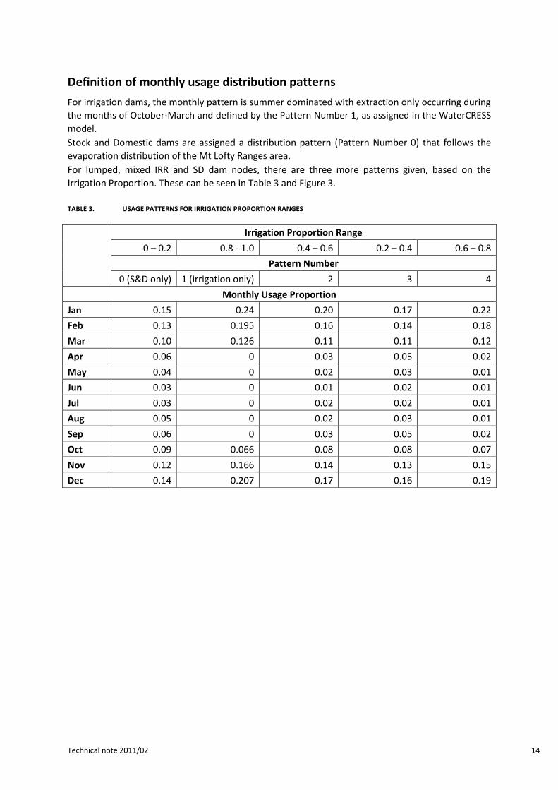
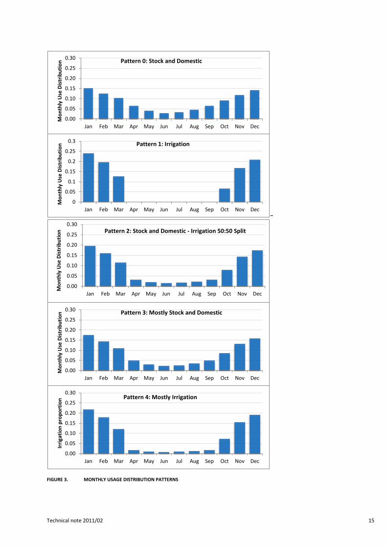
Definition of monthly usage distribution patterns

For irrigation dams, the monthly pattern is summer dominated with extraction only occurring during

the months of October-March and defined by the Pattern Number 1, as assigned in the WaterCRESS

model.

Stock and Domestic dams are assigned a distribution pattern (Pattern Number 0) that follows the

evaporation distribution of the Mt Lofty Ranges area.

For lumped, mixed IRR and SD dam nodes, there are three more patterns given, based on the

Irrigation Proportion. These can be seen in Table 3 and Figure 3.

TABLE 3. USAGE PATTERNS FOR IRRIGATION PROPORTION RANGES

Irrigation Proportion Range

0 – 0.2 0.8 - 1.0 0.4 – 0.6 0.2 – 0.4 0.6 – 0.8

Pattern Number

0 (S&D only) 1 (irrigation only) 2 3 4

Monthly Usage Proportion

Jan 0.15 0.24 0.20 0.17 0.22

Feb 0.13 0.195 0.16 0.14 0.18

Mar 0.10 0.126 0.11 0.11 0.12

Apr 0.06 0 0.03 0.05 0.02

May 0.04 0 0.02 0.03 0.01

Jun 0.03 0 0.01 0.02 0.01

Jul 0.03 0 0.02 0.02 0.01

Aug 0.05 0 0.02 0.03 0.01

Sep 0.06 0 0.03 0.05 0.02

Oct 0.09 0.066 0.08 0.08 0.07

Nov 0.12 0.166 0.14 0.13 0.15

Dec 0.14 0.207 0.17 0.16 0.19


–

FIGURE 3. MONTHLY USAGE DISTRIBUTION PATTERNS

0.00

0.05

0.10

0.15

0.20

0.25

0.30

Jan Feb Mar Apr May Jun Jul Aug Sep Oct Nov Dec

Mo

nth

ly U

se D

istr

ibu

tio

n Pattern 0: Stock and Domestic

0

0.05

0.1

0.15

0.2

0.25

0.3


Mo

nth

ly U

se D

istr

ibu

tio

n Pattern 1: Irrigation

0.00

0.05

0.10

0.15

0.20

0.25

0.30


Mo

nth

ly U

se D

istr

ibu

tio

n

Pattern 2: Stock and Domestic - Irrigation 50:50 Split

0.00

0.05

0.10

0.15

0.20

0.25

0.30


Mo

nth

ly U

se D

istr

ibu

tio

n Pattern 3: Mostly Stock and Domestic

0.00

0.05

0.10

0.15

0.20

0.25

0.30


Irri

gati

on

pro

po

rtio

n Pattern 4: Mostly Irrigation


NET EVAPORATION FROM DAMS

The WaterCRESS model calculates both evaporation and rain falling from the dam surface. When

combined, the difference between evaporation loss and rain on the water surface is termed the net

evaporative loss.

At each time-step the WaterCRESS model calculates a water balance on the dam which is explained

in the steps below: 1. Calculate the surface area from the volume at the previous time step

2. Calculate the evaporative loss, inflows, demand, and rainfall based on the surface area calculated at

(1).

3. Calculate the change in storage, and if storage is greater than the full supply level, spill the remaining

water downstream e.g.

( )

Where:

St = storage to be calculated at current time step (m3)

St-1 = storage at previous time step (m3)

I = inflow rate at current time step (m3/s)

O = outflow rate at the end of the current time step (m3/s)

E = evaporation loss at current time-step (m3/s)

P = rain falling at current time-step (m3/s)

D = water extraction rate (m3/s)

dt = the model time step (s).

Terms E and P are calculated from the current estimate of surface area based on the storage volume

at the previous time step.

Farm dams, as digitised from aerial photography of the region, are initially calculated a maximum

surface area at the level at which the dam ceases to flow. This is usually at the point of the dam

spillway. The surface area of the dam at less than full supply level is calculated using the estimate

described by McMurray (2004)

(

)

Where:

A = Surface area (m2) at volume V

Amax = surface area (m2) at maximum volume

V = volume (ML)

Vmax = Volume at maximum capacity.

For example a 5 ML dam with a maximum surface area of 3300 m2 the relationship of Volume (ML)

to Surface area (m2) would appear as below:


FIGURE 4. FARM DAM AREA-VOLUME RELATIONSHIP AT LESS THAN FULL SUPPLY LEVEL

For a selection of eight dams spread over the four models and split between wet and dry areas for

each catchment, the range of exceedence values are displayed in Figure 4 above. Depending on the

location of the dam, and hence the subsequent rainfall and evaporation regime it is exposed to, the

volume of water in the dam will vary greatly.

TABLE 4. EVAPORATION DETAILS FOR SELECTED FARM DAMS

Node

Dam Volume

(ML)

Mean Annual Runoff (ML/a)

Dam Volume/

Runoff (%)

Mean Annual

Rain (mm)

Mean Pan Evap

(mm)

Net Evap Loss (ML)

Net Evap/Dam

Volume (%)

Summer Evap/Dam

Cap (%)

Angas Wet 77 8.83 185 5% 866 1444 0.65 7% 23%

Angas Dry 6 4.84 45.16 11% 537 1444 1.66 34% 40%

Finniss Wet 299 13.21 77 17% 851 1443 1.33 10% 30%

Finniss Dry 577 16.27 25 65% 670 1536 3.33 20% 26%

Currency Wet 11 248.86 567 44% 896 1371 5.73 2% 16%

Currency Dry 151 3.62 13.88 26% 519 1371 1.27 35% 41%

Bremer Wet 385 75.58 88.1 86% 806 1352 3.8 5% 14%

Bremer Dry 282 10.58 135 8% 558 1590 3.19 30% 33%

As shown in Figure 5, at the 50th percentile exceeded value (median), dams ranged from being full to

only 56% of full supply. There are other factors involved in this dynamic including the rate and

regime of water extraction from a farm dam, then amount of water diverted to the dam or bypassed

around the dam, and the amount of runoff (in turn related to catchment area and runoff).

0

500

1000

1500

2000

2500

3000

3500

0 1 2 3 4 5 6

Surf

ace

Are

a (m

2)

Dam Volume (ML)

Farm Dam Area-Volume Relationship (McMurray, 2004)


FIGURE 5. RANGE OF DAM VOLUME EXCEEDENCES

In order to gain an understanding of the overall water balances for these data, statistics have been

calculated at the catchment scale with the WaterCRESS model being able to aggregate the

calculations of each farm dam in the output file. This enables estimates to be made including; net

evaporation loss, precipitation, dam volume, and extraction.

Results for these are given in the following section which includes an assessment of the seasonal

estimate of net loss from farm dams for the months of November to May inclusive. These months

cover those identified by Van Laarhoven et al (2009), as covering the critical flow seasons; Low Flow

Season, Transition season 1 (Low to High), and Transition Season 2 (High to Low).

Figure 6 below shows the mean monthly storage volumes calculated in all dams, comprising a

mixture of demands (refer to section on Water Use) highlighting the decreasing storage volume

between November and April inclusive.

FIGURE 6. MEAN MONTHLY STORAGE VOLUME OF EMLR FARM DAMS

0

2000

4000

6000

8000

10000

12000

14000


Me

na

Mo

nth

ly S

tora

ge

Vo

lum

e (

ML)

Month

Mean Monthly Storage Volume


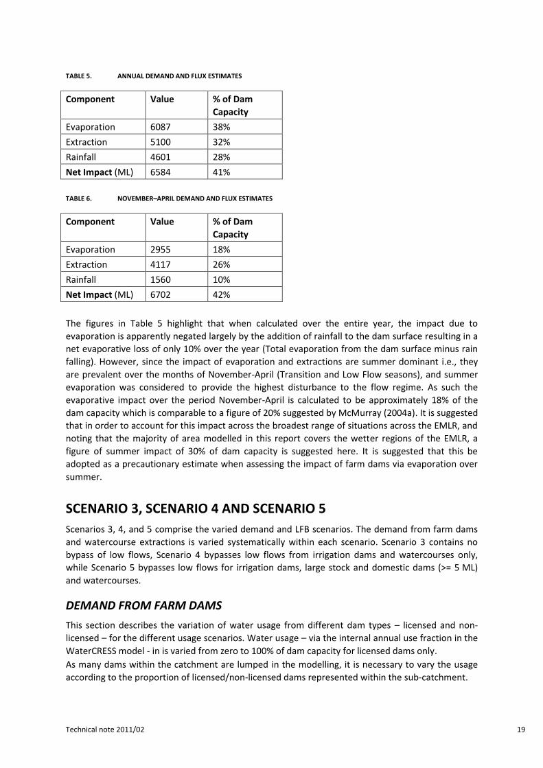
TABLE 5. ANNUAL DEMAND AND FLUX ESTIMATES

Component Value % of Dam

Capacity

Evaporation 6087 38%

Extraction 5100 32%

Rainfall 4601 28%

Net Impact (ML) 6584 41%

TABLE 6. NOVEMBER–APRIL DEMAND AND FLUX ESTIMATES

Component Value % of Dam

Capacity

Evaporation 2955 18%

Extraction 4117 26%

Rainfall 1560 10%

Net Impact (ML) 6702 42%

The figures in Table 5 highlight that when calculated over the entire year, the impact due to

evaporation is apparently negated largely by the addition of rainfall to the dam surface resulting in a

net evaporative loss of only 10% over the year (Total evaporation from the dam surface minus rain

falling). However, since the impact of evaporation and extractions are summer dominant i.e., they

are prevalent over the months of November-April (Transition and Low Flow seasons), and summer

evaporation was considered to provide the highest disturbance to the flow regime. As such the

evaporative impact over the period November-April is calculated to be approximately 18% of the

dam capacity which is comparable to a figure of 20% suggested by McMurray (2004a). It is suggested

that in order to account for this impact across the broadest range of situations across the EMLR, and

noting that the majority of area modelled in this report covers the wetter regions of the EMLR, a

figure of summer impact of 30% of dam capacity is suggested here. It is suggested that this be

adopted as a precautionary estimate when assessing the impact of farm dams via evaporation over

summer.

SCENARIO 3, SCENARIO 4 AND SCENARIO 5

Scenarios 3, 4, and 5 comprise the varied demand and LFB scenarios. The demand from farm dams

and watercourse extractions is varied systematically within each scenario. Scenario 3 contains no

bypass of low flows, Scenario 4 bypasses low flows from irrigation dams and watercourses only,

while Scenario 5 bypasses low flows for irrigation dams, large stock and domestic dams (>= 5 ML)

and watercourses.

DEMAND FROM FARM DAMS

This section describes the variation of water usage from different dam types – licensed and non-

licensed – for the different usage scenarios. Water usage – via the internal annual use fraction in the

WaterCRESS model - in is varied from zero to 100% of dam capacity for licensed dams only.

As many dams within the catchment are lumped in the modelling, it is necessary to vary the usage

according to the proportion of licensed/non-licensed dams represented within the sub-catchment.


Variation of Usage from Lumped Dam Nodes where there is a combination of Licensed Irrigation Dams and Non-licensed Stock and Domestic dams

As some sub-catchments have a combination of licensed and non-licensed dams that may require

LFB, there is a requirement to fix the level of usage from non-licensed 5 ML dams (and smaller SD

dams) at 30% of the dam capacity (this is a major assumption of all modelling of SD dams to date)

and vary the demand from irrigation dams and watercourse extractions.

For the demand scenarios i.e., varying demand from 0 to 100% for licensable dams it is necessary to

separate out the total volume of irrigation dams from stock and domestic dams.

The irrigation proportion is defined as the total capacity of identified irrigation (licensed) dams

divided by the total capacity of dams for the modelled sub-catchment.

EQUATION 2. VARIABLE DEMAND CALCULATION FOR MIXED SOURCE EXTRACTIONS

( ) ( )

This simplifies to:

( )

Where:

un = variable demand fraction (n = 0, 0.1, 0.2....0.9, 1.0)

IP = irrigation proportion

SDP = Stock and Domestic Proportion (1 – IP)

SD30 = Fixed demand proportion for stock and domestic dams of 30%

UFn = Combined use fraction at variable demand n

TABLE 7. EXAMPLE FOR A 50% IRRIGATION PROPORTION

Irrigation Proportion (IP) 0.5

Stock and Domestic

Proportion (SDP)

0.5

Variable Irrigation

Proportion (un)

un times IP SDP times fixed 30%

(SD30)

Total Demand Fraction

(UFn)

0 0 0.15 0.15

0.1 0.05 0.15 0.2

0.2 0.1 0.15 0.25

0.3 0.15 0.15 0.3

0.4 0.2 0.15 0.35

0.5 0.25 0.15 0.4

0.6 0.3 0.15 0.45

0.7 0.35 0.15 0.5

0.8 0.4 0.15 0.55

0.9 0.45 0.15 0.6

1 0.5 0.15 0.65


VARIATION OF DEMAND FROM WATERCOURSE EXTRACTIONS AND LOW FLOW BYPASS CONDITIONS.

Water usage from watercourse extractions in the models was also varied between 0 and 100% of the

original estimates1.

To allow the bypassing of low-flows past watercourse extractions at the defined TFR, the original set-

up of the model was required to be altered.

Previously watercourse extractions were enabled in the model by inserting a stream storage node,

and extracting water from the node via a Text File Demand Node. This situation did not allow for the

bypassing of low-flows as may be required under the proposed water allocation plan for the EMLR.

To allow this to happen, a weir node (Number 2 in Figure 7) was inserted above the stream storage

node (Number 5 in Figure 7) and the diversion off-take (the pink line) was directed to the stream

node. The main branch of the weir node is connected downstream in the direction of flow. The weir

node allows a constant “base flow-to-pass” rate to be applied which is analogous to the Threshold

Flow Rate. As for dams, the effect is to bypass flows along the main branch of the model. Refer to

Figure 7 below for an example of how the model is constructed.

FIGURE 7. WATERCOURSE EXTRACTION SET-UP WATERCRESS MODEL

The “baseflow (or low flows) to pass” rate is calculated in the same manner as the TFR for dams.

(Upstream area times UFTR)

1 Watercourse extraction estimates were supplied by Resource Allocation Division in May 2010 at the SWMZ

scale


Watercourse extraction estimates: Catchment Scale

Watercourse demand estimates were supplied by the Water Planning and Management Division

(WPMD) of DFW and are categorized by catchment total demand in Table 6 below. It should be

noted that these figures are best estimates at the time of this report and could change as more

information becomes available during the licensing process of the EMLR WAP.

TABLE 8. CATCHMENT-SCALE WATERCOURSE DEMAND ESTIMATES

Catchment Watercourse Demand Estimate (ML/a)

Angas 873

Bremer 1856

Currency 290

Finniss 631

Selection of sub-catchments for low flow releases

The total number of modelled sub-catchments across the five catchments is 932.

Using the criteria of Stock and Domestic, Irrigation or Stock and Domestic larger than 5 ML, 382 of

932 model dam nodes have a LFB applied. The break down by catchment is in Table 9.

TABLE 9. SUB-CATCHMENTS SELECTED FOR LOW FLOW BYPASS

Scenario 5*: Sub-

cats. to Bypass Low

Flows

Scenario 4**: Sub-cats.

containing only Irrigation Dams

Sub-cats. containing at

least one dam >= 5 ML

Angas 79 56 78

Bremer 137 94 136

Currency 28 33 23

Finniss 128 116 127

Total 372 299 364

*Varied demand on irrigation dams – low flow releases on irrigation dams and dams with a

capacity of 5 ML or greater

**Varied demand on irrigation dams – low flow releases on irrigation dams only

Description of programs and data required to process inputs and outputs

Geographic Information System (GIS)

A GIS was used to identify the location of Farm Dams, model sub-catchments and water extractions.

This information was used to determine the location of sub-catchments required to bypass low-

flows, and also to determine the ratio of Stock and Domestic use to Irrigation use in each sub-

catchment.

Excel Spreadsheets: 1. EWR_Scenarios2010.xlsm: Outputs and macros relating to base node information and EWR Metric result

summaries

2. Use_Scenario.xlsm: Spreadsheet and macros used for running LFB and Demand Scenarios for Scenario 3

3. LFB_Use_ScenarioNewLFBIRR.xlsm: Spreadsheet and macros used for running LFB and Demand Scenarios for

Scenario 4


4. LFB_Use_Scenario.xlsm: Spreadsheet and macros used for running LFB and Demand Scenarios for Scenario 5.

VBA programs

The analysis of these LFB and Demand scenarios, and the management of the output data sets relies

on the use of several VBA (Visual Basic for Applications) scripts that allow for the processing of large

numbers of scenario runs and output data. The table below describes: 1. The location (spreadsheet) in which the script resides

2. The order in which to run the scripts

3. Any other required data e.g. an open excel worksheet.

The full macro name is of the form:

[Spreadsheet Name]![Module Name].[Procedure Name]

TABLE 10. LIST OF SCRIPTS TO RUN EWR SCENARIO ANALYSIS

Step Full Macro Name (includes base spreadsheet as the prefix) Main Spreadsheet Description

1 Use_Scenario.xlsm!NoDamsScenario. run_nodams_scenario() Use_Scenario.xlsm Sets all demands

and dam volumes to

zero, runs model

and saves results.

2 Use_Scenario.xlsm!UseScenarios. usage_main() Use_Scenario.xlsm Runs through the

demand scenarios

for Scenario 3, and

saves outputs.

3 LFB_Use_Scenario.xlsm!UpdateTFR. UpdateUTFR_Main() LFB_Use_Scenario.xlsm Sets the Threshold

Flow rates for all

applicable dams and

extraction nodes.

3 LFB_Use_Scenario.xlsm!LFBUseMain.LFB_Use_Main() Runs through the

demand scenarios

for Scenario 4 and 5,

and saves outputs.

5 LFB_Use_Scenario.xlsm!SetTFRtoZero.ResetTFRtoZero_Main() LFB_Use_Scenario.xlsm Resets all Threshold

Flow rates back to

Zero.

6 EWR_Scenarios2010.xlsm!GetSummaryData.getdata_main() EWR_Scenarios2010.xlsm Collates model

summary output

files.

7 EWR_Scenarios2010.xlsm!update_output_node() EWR_Scenarios2010.xlsm Collates all node

information from

the model in this

spreadsheet.


WaterCRESS Model Platform

These models are developed and run using the WaterCRESS model platform, which calculates water

balances for catchments, storages and extractions on a daily time step.

The WaterCRESS model executables used in this report are:

1.

2.


FIGURE 8. ANGAS RIVER TESTING SITES AND LFB SELECTION SCENARIO 4


FIGURE 9. BREMER RIVER TESTING SITES AND LFB SELECTION SCENARIO 4


FIGURE 10. CURRENCY CREEK TESTING SITES AND LFB SELECTION SCENARIO 4


FIGURE 11. FINNISS RIVER TESTING SITES AND LFB SELECTION SCENARIO 4


FIGURE 12. ANGAS RIVER TESTING SITES AND LFB SELECTION SCENARIO 5


FIGURE 13. BREMER RIVER TESTING SITES AND LFB SELECTION SCENARIO 5


FIGURE 14. CURRENCY CREEK TESTING SITES AND LFB SELECTION SCENARIO 5


FIGURE 15. FINNISS RIVER TESTING SITES AND LFB SELECTION SCENARIO 5


RESULTS

FARM DAMS

There are a total of 7103 dams counted in the EMLR PWRA with a total estimated capacity of 18.4 GL.

Dams with a capacity of at least 5 ML account for 10% (692) of the total number dams with a combined

capacity accounting for 64% (11.8 GL) of the total capacity.

Licensed dams:

There were a total of 558 licensed dams identified for this report, comprising an estimated capacity of

6674 ML. Of these 558 dams, 251 are at least 5 ML in capacity.

Non-licensed dams:

A total of 6545 non-licensed dams were identified in this report comprising an estimated capacity of

11,701ML. Of these dams, 441 are at least 5 ML in capacity.

Dams within the model domain:

Of the total 7103 dams inside the EMLR PWRA, 5546 fall within the model domain (Figure 1) of the 4

hydrological models. These dams represent a total of 14,930 ML of storage, which is 81% of the total.

There are 472 licensed dams identified and 340 additional Stock and Domestic dams with a capacity of

5 ML or greater. These two categories represent ~75% of the total modelled dam capacity within the

five modelled catchments.

MODEL SUB-CATCHMENTS

For the scenario where only Irrigation Dams are required to bypass low flows, 299 of a total 857 model sub-

catchments are selected for LFB.

For the scenario where large stock and domestic dams (=> 5 ML) are also required to bypass low flows, 364

of 857 model sub-catchments are selected for LFB.

TABLE 11. MODEL SUB-CATCHMENTS SELECTED FOR LFB

Scenario 5*:

Sub-cats to

Bypass Low

Flows

Scenario 4**:

Sub-cats

containing

only irrigation

dams

Sub-cats

containing at

least one dam >=

5 ML

Angas 79 56 78

Bremer 137 94 136

Currency 28 33 23

Finniss 128 116 127

Total 372 299 364

*Varied demand on irrigation dams – low flow releases on irrigation dams and dams with a capacity of

5 ML or greater

** Varied demand on irrigation dams – low flow releases on irrigation dams only

WATER USE ESTIMATES FOR DEMAND SCENARIOS

Water use, expressed as a percentage of total runoff (not including stream losses) is reported in Table 12

below. Base case – that is, the current estimate of water usage is highest in the Angas River catchment at


15% of the runoff generated over the catchment, whilst the Finniss River records the lowest overall

percentage of usage at 7%.

It should be noted that these figure are reported at a whole of catchment scale, and water usage will be

higher at smaller scales within the catchment.

TABLE 12. WATER USAGE AS PERCENT OF TOTAL CATCHMENT RUNOFF FOR VARIOUS DEMAND SCENARIOS

De

man

d S

cen

ario

Angas Bremer Currency Finniss Tookayerta

No

LFB

LFB

Irr.

Dam

s O

nly

LFB

Irr.

an

d >

= 5

ML

No

LFB

LFB

Irr.

Dam

s O

nly

LFB

Irr.

an

d >

= 5

ML

No

LFB

LFB

Irr.

Dam

s O

nly

LFB

Irr.

an

d >

= 5

ML

No

LFB

LFB

Irr.

Dam

s O

nly

LFB

Irr.

an

d >

= 5

ML

No

LFB

LFB

Irr.

Dam

s O

nly

LFB

Irr.

an

d >

= 5

ML

Base 15 13 13 12 11 11 10 8 8 7 5 5 12 12 12

Use 0 6 5 5 5 5 5 2 2 2 2 2 2 1 1 1

Use 10 7 7 7 7 7 7 4 4 4 3 3 3 2 2 2

Use 20 9 9 9 8 8 8 5 5 5 4 3 3 3 3 3

Use 30 10 10 10 9 8 8 6 6 6 4 4 4 5 5 5

Use 40 12 11 11 10 9 9 7 7 7 5 5 5 6 6 6

Use 50 13 12 12 11 10 10 9 8 8 6 5 5 7 7 7

Use 60 15 13 13 12 10 10 10 8 8 7 6 6 8 8 8

Use 70 16 14 14 12 11 11 11 9 9 7 6 6 10 9 9

Use 80 17 15 15 13 11 11 12 10 10 8 7 7 11 10 11

Use 90 18 15 15 14 12 12 13 11 11 8 7 7 12 12 12

Use 100 19 16 16 14 12 12 14 11 11 9 7 7 13 13 13

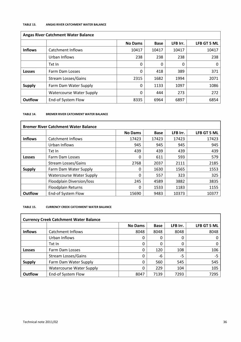
CATCHMENT WATER BALANCES

Mean Annual Catchment water balances are estimated here for each catchment for the following

scenarios: 1. Scenario 1: No Dams or extractions

2. Scenario 2: Base (Current) – use scenario with no LFB

3. Scenario 4: Base (Current) – use with LFB on Irrigation Dam sub-catchments only

4. Scenario 5: Base (Current) – use with LFB on Irrigation Dam and Large SD Dam sub-catchments.

These data represent the mean annual water balance for the period 1971-2006.


TABLE 13. ANGAS RIVER CATCHMENT WATER BALANCE

Angas River Catchment Water Balance

No Dams Base LFB Irr. LFB GT 5 ML

Inflows Catchment Inflows 10417 10417 10417 10417

Urban Inflows 238 238 238 238

Txt In 0 0 0 0

Losses Farm Dam Losses 0 418 389 371

Stream Losses/Gains 2315 1682 1994 2071

Supply Farm Dam Water Supply 0 1133 1097 1086

Watercourse Water Supply 0 444 273 272

Outflow End-of System Flow 8335 6964 6897 6854

TABLE 14. BREMER RIVER CATCHMENT WATER BALANCE

Bremer River Catchment Water Balance




Txt In 439 439 439 439


Stream Losses/Gains 2768 2037 2111 2185



Floodplain Diversion/loss 245 4589 3882 3835

Floodplain Returns 0 1533 1183 1155


TABLE 15. CURRENCY CREEK CATCHMENT WATER BALANCE

Currency Creek Catchment Water Balance




Txt In 0 0 0 0


Stream Losses/Gains 0 -6 -5 -5





TABLE 16. FINNISS RIVER CATCHMENT WATER BALANCE

Finniss River Catchment Water Balance




Txt In 0 0 0 0


Stream Losses/Gains -42 -56 -46 -44




Based on the catchment water balances presented in Tables 12 to 16, there would be a total of 2% increase

to end of system flows for both Scenarios 4 and 5 as opposed to Scenario 3 (Current). There appears to be

little difference in the overall end-of-system flows between the two LFB scenarios. Whilst this may suggest

there is little benefit in applying Scenario 5 over Scenario 4 in terms of mean annual water balances, it

should be noted that the determination of Environmental Water Requirements uses a more detailed set of

criteria to assess this against. These criteria are not discussed further in this report as they are the subject

of a previous report on the determination of the EWR of the MLR (VanLaarhoven, et al., 2009).

In the Angas River catchment, there appears to be a negative difference in the end of system flow with the

Low Flow Bypass scenarios when compared with Scenario 3. This can be largely attributed to the method

employed to simulate stream losses in the lower reaches of the model which use a linear relationship to

model loss. In the event that low flow releases enable flow to travel through to the Angas Plains section of

the model, some of this low-flow is simulated as being lost to the stream bed. This flow would be in

addition to any losses currently occurring in the model if the flow occurs at a time in which the stream did

not previously flow.

EFFECT OF LFB AND DEMAND SCENARIOS ON DAILY FLOW

Results in this section are presented for two testing sites – B18 and F15. These results are intended to

demonstrate the effect on the daily flow regime of bypassing low flows from farm dams and setting

threshold flow levels on watercourse extractions for the two bypass scenarios in catchments with different

flow regimes ranging from dry (B18) to wet (F15).


Site B18 Results

FIGURE 16. MODEL LAYOUT COMPARISON OF SCENARIOS 4 AND 5 FOR EWR SITE B18 IN THE UPPER BREMER RIVER

TABLE 17. EWR SITE DETAILS FOR B18 IN THE UPPER BREMER RIVER

Catchment Bremer River

Zone NAME B18

Upstream Adjusted Runoff (KL) 2736557

Upstream Dam Farm Dam Capacity (KL) 645341

Dam Capacity /Upstream Runoff 24%

Dam Density (ML/km2) 11.2

Reach Type Wet Upper Pool Riffle


TABLE 18. DAILY FLOW STATISTICS FOR EWR SITE B18 IN THE UPPER BREMER RIVER

Daily Flow Statistic (ML/day) Scenario 1 Scenario 2 Scenario 4 Scenario 5

Mean 7.85 6.96 7.00 7.00

10th Percentile 0.00 0.00 0.00 0.00

20th Percentile 0.00 0.00 0.00 0.00

30th Percentile 0.00 0.00 0.00 0.00

40th Percentile 0.00 0.00 0.00 0.00

50th Percentile 0.05 0.00 0.00 0.00

60th Percentile 0.23 0.00 0.00 0.00

70th Percentile 0.73 0.00 0.01 0.19

80th Percentile 2.05 0.76 1.17 1.42

90th Percentile 6.65 4.61 4.91 5.03

FIGURE 17. FLOW DURATION CURVES FOR EWR SITE B18 IN THE UPPER BREMER RIVER

Comprising the upper reaches of the Bremer River with rainfall of around 500mm, EWR zone B18 under the

pre-development scenario would flow for less than 50% of the year. Under the current-use scenario, flow is

reduced in this reach to around 20% of the time during an average year.

Figure 17 shows an improvement in both Scenarios 4 and 5 with daily flows in both scenarios increasing by

around 10 percent in duration. The improvement in flows below 1ML/day is considerable for both scenarios

in relative terms showing a 21% improvement in the 80th Percentile Flow (Table 17).

Note that modelling of very low flows in dry ephemeral catchments generally entails a high level of

uncertainty, and as such the results should be taken as an indicative response for a low rainfall ephemeral

stream reach. For calibration details of the Bremer River model please refer to the modelling report for that

catchment. (Alcorn, 2008)

0.1

1

10

100

1000

10000

0% 20% 40% 60% 80% 100%

Dai

ly F

low

(M

L/d

ay)

% of time flow exceeded

Site B18 Flow Duration

Scenario 1

Scenario 4

Base_LFB

Base


Site F15 Results

FIGURE 18. MODEL LAYOUT COMPARISON OF SCENARIOS 4 AND 5 FOR EWR SITE F15 IN THE LOWER FINNISS RIVER

TABLE 19. EWR SITE DETAILS FOR F15 IN THE LOWER FINNISS RIVER

Catchment Bremer River

Zone NAME F15

Upstream Adjusted Runoff (KL) 38,194,644

Upstream Dam Farm Dam Capacity (KL) 5,006,231

Dam Capacity /Upstream Runoff 13%

Dam Density (ML/km2) 13.3

Reach Type Lowland with Floodplain

TABLE 20. DAILY FLOW STATISTICS FOR EWR SITE F15 IN THE LOWER FINNISS RIVER


Mean 100.94 92.84 94.26 94.31

10th Percentile 2.99 0.00 1.51 1.88

20th Percentile 6.05 0.67 3.14 3.77

30th Percentile 9.91 2.73 5.95 6.86

40th Percentile 16.22 7.14 10.21 11.35

50th Percentile 26.48 15.33 18.22 19.41

60th Percentile 42.58 31.69 31.48 32.67



70th Percentile 66.76 55.74 53.43 53.57

80th Percentile 117.19 107.63 96.04 95.15

90th Percentile 264.16 251.10 247.33 245.11

FIGURE 19. FLOW DURATION CURVES FOR EWR SITE F15 IN THE LOWER FINNISS RIVER

Site F15 drains almost the entire Finniss River catchment and so shows the full catchment scale impact of

bypassing low flows from farm dams and watercourse extractions. The flow duration indicates that under

current conditions, the Lower Finniss flows for just over 80% of the year, whilst under adjusted conditions it

may flow for the entire year. The bypassing of low flows would greatly improve the duration of flows up to

around 10 ML/day.

Interestingly, bypassing low flows would have the effect of actually decreasing some high flows in the range

of 100 ML/day or greater. The cause of this effect is that allowing low flows to bypass the system early in

the season can delay the fill of the dam to its maximum capacity. In doing so, the spill of water is effectively

spread over a longer period, thereby reducing the size of some peak flows.

0.1

1

10

100

1000

10000

0% 20% 40% 60% 80% 100%

Dai

ly F

low

(M

L/d

ay)

% of time flow exceeded

Site F15 Flow Duration

Scenario 1

Scenario 4

Base_LFB

Base


REFERENCES

Alcorn M. Surface Water Assessment of the Bremer River Catchment [Report] : Report 2008/13. -

Adelaide : SA Government, 2008.

Alcorn M. Updates to the capacities of the Surface Water Resource of the Eastern Mount Lofty Ranges:

2010 [Report]. - Adelaide : Department For Water, 2010/04.

Alcorn M. Savadamuthu S. Murdoch B. Capacity of the surface water resource of the Eastern Mount Lofty

Ranges [Report]. - Adelaide : Department of Water land and Biodiversity Conservation, 2008. - 2008/23.

Alcorn M. Surface Water Assessment of the Currency Creek Catchment [Book]. - South Australia :

Department for Water Land and Biodiversity, 2006.

McMurray D. Assessment of water use from farm dams in the Mount Lofty Ranges, South Australia

[Report] : Report 2004/02. - Adelaide : SA Government, 2004.

McMurray D. Farm Dam volume estimations from simple geometric relationships [Report] : Report

2004/48. - Adelaide : SA Government, 2004.

Savadamuthu K. Streamflow in the Upper Finniss Catchment [Report] : Report 2003/13. - Adelaide : SA

Government, 2003.

Savadamuthu K. Surface Water Assessment of the the Upper Angas sub-catchment [Report] : Report

2006/09. - Adelaide : SA Government, 2006.

Savadamuthu K. Surface Water Assessment of the Tookayerta Catchment [Report] : Report 2004/23. -

Adelaide : SA Government, 2004.

VanLaarhoven J. and Van Der Wielen M. Environmental water requirements for the Mount Lofty Ranges

prescribed water resources areas [Report]. - Adelaide : Department of Water, Land and Biodiversity

Conservation & South Australian Murray-Darling Basin NRM Board, 2009.

technical note 2011/02 - waterconnect.sa.gov.au

Documents