technical report 8: model development and application...
TRANSCRIPT

250 South Orange Avenue, Suite 200, Orlando, FL 32801 | 407-481-5672
www.metroplanorlando.com | MetroPlan Orlando | @metroplan_orl
2040 Long Range Transportation Plan
Technical Report 8:
Model Development and Application
Guidelines Final Adopted Plan
January 2016

2040 Long Range Transportation Plan: Technical Report 8 i
Table of Contents
1.0 INTRODUCTION ...................................................................... 1 1.1 Report Overview ......................................................... 1 1.2 Background of Year 2009 Model ....................................... 1 1.3 Florida’s Standard Model ............................................... 2 1.3.1 Highway and Transit Options ................................ 2 1.3.2 OUATS Model Process......................................... 5 2.0 EXTERNAL TRIP MODEL ............................................................. 5 2.1 External Trip Development ........................................... 10 2.1.1 Auto External Trips ......................................... 10 2.1.2 Truck External Trips ........................................ 10 2.1.3 Special Attraction External Trips ......................... 10 2.2 External Trip Summary ............................................... 11 3.0 TRIP GENERATION MODEL ....................................................... 11 3.1 Trip Generation Model Overview .................................... 12 3.2 Trip Generation Model Input Data and Parameters .............. 15 3.2.1 Socioeconomic Data ........................................ 15 3.2.2 Special Attractions Socio-Economic Data................ 16 3.2.3 Input Variables and Parameters .......................... 17 3.3 Truck Generation Program ............................................ 20 3.4 Special Attractions Program .......................................... 20 3.4.1 Special Trip Generation Methodology .................... 20 3.4.2 Special Attractions Program Summary ................... 21 3.5 Trip Generation Results ............................................... 21 4.0 TRIP DISTRIBUTION MODEL ...................................................... 23 4.1 Trip Distribution Model Overview .................................... 23 4.2 Gravity Model Methodology and Operation ......................... 24 4.3 Gravity Model Inputs and Variables .................................. 26 4.4 Special Trips Development............................................ 26 4.4.1 Special External Trip Development ...................... 26 4.4.2 Special Internal Trip Development ....................... 27 4.5 Trip Distribution Results .............................................. 28

2040 Long Range Transportation Plan: Technical Report 8 ii
Table of Contents (Cont’d) 5.0 MODE CHOICE MODEL............................................................. 29 5.1 Default Mode Choice Model .......................................... 31 5.2 Mode Choice Model Operation ....................................... 32 5.3 Mode Choice Special Purposes ....................................... 32 5.4 Changes to the Mode Choice Program .............................. 33 5.5 Mode Choice Output .................................................. 34 6.0 HIGHWAY ASSIGNMENT AND EVALUATION MODELS ........................... 36 6.1 Highway Assignment Model .......................................... 36 6.1.1 Highway Assignment Model Overview .................... 36 6.1.2 Highway Assignment Model Methodology & Operation 37 6.2 Highway Assignment Results ......................................... 37 6.3 Highway Evaluation Model ........................................... 37 6.3.1 Highway Evaluation Model Overview ..................... 37 6.3.2 Highway Evaluation Model Methodology & Operation . 39 6.4 Highway Evaluation Results .......................................... 42 7.0 TRANSIT ASSIGNMENT MODEL ................................................... 44 7.1 Transit Network Development ....................................... 45 7.2 Transit Assignment Model Methodology & Operation ............ 45 7.3 Transit Assignment Results ........................................... 46 8.0 APPLICATION GUIDELINES ........................................................ 49 8.1 Minimum System Requirements ..................................... 49 8.2 Directory Structure .................................................... 49 8.2.1 Base Folder .................................................. 50 8.2.2 Parameters Folder .......................................... 52 8.2.3 User.prg Folder .............................................. 52 8.2.4 Applications Folder ......................................... 53 8.2.5 GIS Folder .................................................... 53 8.3 Scenario Setup ......................................................... 53 8.3.1 Scenario Selection .......................................... 53 8.3.2 Creating a Scenario ......................................... 54 8.4 Running the Model ..................................................... 56

2040 Long Range Transportation Plan: Technical Report 8 iii
LIST OF TABLES
1. External Station Trip Purposes ....................................................... 7 2. External Station Numbers and Locations ............................................ 8 3. Year 2009 Production Variables Summary ........................................ 15 4. Year 2009 Attraction Variables Summary ........................................ 16 5. Year 2000 Special Generators ...................................................... 16 6. Year 2009 Special Attraction Trip Generation Attractions Summary ......... 17 7. Year 2009 Special Attraction Trip Generation Productions Summary ........ 18 8. Year 2000 CTPP Journey-to-Work Trips ........................................... 19 9. Special Attractions Productions and Attractions Trip Purposes ............... 21 10. Year 2009 Trip Generation Model Output ....................................... 22 11. Year 2009 Trip Generation Statistics ............................................. 23 12. Daily Trip Distribution Summary ................................................. 28 13. Total Mode Choice Output ........................................................ 35 14. Traffic Assignment Accuracy Levels ............................................. 41 15. Screenline/Cutline Summaries ................................................... 42 16. HEVAL.PRN Statistics .............................................................. 43 17. Percent Root Mean Squared Error (% RMSE) Summary ....................... 43 18. Transit Assignment Ridership by Route For 2009 ............................... 47
LIST OF FIGURES
1. Geographic Area Covered by the OUATS Model .................................... 3 2. Overall Model Chain .................................................................... 4 3. Model Flow Chart ....................................................................... 6 4. External Station Locations ............................................................ 9 5. TRIP GENERATION Flow Chart ...................................................... 14 6. TRIP DISTRIBUTION Flow Chart .................................................... 24 7. MODE Flow Chart .................................................................... 29 8. OUATS Mode Choice Nesting Structure ........................................... 30 9. HIGHWAY ASSIGNMENT Flow Chart ................................................ 36 10. Time Penalty Locations ............................................................ 38 11. HIGHWAY EVALUATION Flow Chart .............................................. 39 12. Year 2009 Screenline and Cutline Locations ................................... 40 13. TRANSIT ASSIGNMENT Flow Chart ................................................ 44 14. TRANSIT ASSIGNMENT Results Visualization .................................... 46 15. File Folder Tree .................................................................... 50

2040 Long Range Transportation Plan: Technical Report 8 iv
LIST OF FIGURES (Cont’d) 16. Main OUATS Model Screen ......................................................... 52 17. User Specific Parameters Screen ................................................. 54 18. Scenario Tree .................................................................... 55
APPENDICES Appendix A: External Trips ............................................................ 57
Appendix B: Socio-Economic Data ................................................... 60
Appendix C: Trip Generation ......................................................... 73
Appendix D: Mode Choice ............................................................. 82

2040 Long Range Transportation Plan: Technical Report 8 1
1.0 Introduction
MetroPlan Orlando, as part of the Year 2040 Long Range Transportation Plan (LRTP), updated the Orlando Urban Area Transportation Study (OUATS) travel demand forecasting model in Phase I of the project. The previous base year (2004) model validation used for the 2030 LRTP was used as the starting point for the year 2009 model validation effort. This Technical Report No. 8, titled "Model Development and Application Guidelines," is designed to document the Year 2009 OUATS model validation and calibration process. In addition, information regarding model setup and use is included as an application guideline.
Report Overview This section (Section 1.0) provides the general introduction for this Technical Report. Section 2.0 provides details of the external trip model, the external trips development, and the results of the OUATS year 2004 external trips. Section 3.0 provides details of the trip generation process. Section 4.0 provides details of the trip distribution process. Section 5.0 provides information regarding the mode choice model. Section 6.0 presents information regarding the highway assignment process and evaluation models. Section 7.0 details the transit assignment process. Sections 3.0 through 7.0 include the incorporation of the Low, Medium, and High income level procedure developed as part of the “Trip Characteristics Study” done by Leftwich Consulting Engineers, Inc. for MetroPlan Orlando as part of the 2030 LRTP model development. Section 8.0 details the proper steps to take into consideration to correctly use the travel demand model.
Background of the Year 2009 Model The Orlando Urban Area Transportation Study (OUATS) year 2009 model includes the geographic area covered by the Orlando Urban Area (i.e., Orange, Osceola and Seminole counties) as well as the western portion of the Volusia County network, the Lake County network, and northeastern portion of the Polk County network (see Figure 1). As part of the 2030 LRTP model validation effort, the model went through a complete overhaul. The base year 2000 model, which was in place prior to the 2030 LRTP, referenced the Florida Standard Urban Transportation Model Structure (FSUTMS) procedures using the TRANPLAN suite of programs. The 2030 LRTP base year 2004 model was then updated to use the CUBE/Voyager software (licensed by Citilabs) that the State of Florida has adopted as the travel demand models “engine” across the state. Both Highway and Transit networks, the basis for this model, were coordinated with Geographic Information System (GIS) data using

2040 Long Range Transportation Plan: Technical Report 8 2
the CUBE/Voyager software. The CUBE/Voyager software continues to be the premise for the base year 2009 model validation performed for the 2040 LRTP model development.
1.3 Florida's Standard Model
The Florida Standard Urban Transportation Model Structure (FSUTMS), developed and maintained by the Florida Department of Transportation (FDOT), is the standard model process used for transportation planning in Florida. FSUTMS is a versatile process that can be used to model highway and transit systems. It provides four (4) options relative to the modes of transportation to be considered: Highway-Only Process, Single-Path Transit Process, Multi-Path Transit Process, and Multi-Path Multi-Period Transit Process.
1.3.1 Highway and Transit Options The Highway-Only Process is used in smaller urbanized areas that either do not currently have transit service or have very minor transit that cannot be effectively modeled. The Single-Path Transit Process is used in small to medium urbanized areas with no appreciable difference between the peak and off-peak transit routes and route headways. The Multi-Path Single-Period Transit Process is applied to urbanized areas that have expanded systems, and several types of transit services, with no significant difference in the peak and off-peak services. Finally, the Multi-Path Multi-Period Transit Process is used for urbanized areas that have expanded systems and several types of transit services with significant difference in the peak and off-peak period services. The OUATS model follows the multi-path multi-period process. The overall model chain can be summarized as depicted in Figure 2.

2040 Long Range Transportation Plan: Technical Report 8 3
FIGURE 1: GEOGRAPHIC AREA COVERED BY THE OUATS MODEL

2040 Long Range Transportation Plan: Technical Report 8 4
FIGURE 2: OVERALL MODEL CHAIN

2040 Long Range Transportation Plan: Technical Report 8 5
1.3.2 OUATS Model Process The OUATS model has evolved over the past 30 years to a modified version of the multi-path, multi-period process that includes trip purposes for special attractions (such as Walt Disney World, Universal Studios, Sea World, Orlando International Airport, the Orange County Convention Center, etc.). In addition, a truck model was incorporated during the year 2000 validation effort. For the year 2004 validation effort a “Trip Characteristics” component was added to the process. For the home-based work (HBW) purpose, the generation of productions and attractions is based on three (3) income level groups (i.e. Low, Medium, and High), that are based on property values. Validation/Calibration of the OUATS model was performed using the Nested Logit Multi-Path, Multi-Period Transit process. This process is shown in the OUATS Model Flow (see Figure 3) from the CUBE/Voyager software. The main, also referred to as the Parent level, application modules of the OUATS CUBE/Voyager model are: TRIP GENERATION – Builds external trip table and generates internal trips (productions
and attractions) NETWORK – Highway network processing and paths DISTRIBUTION – Gravity models, pre-mode choice, and pre-highway assignment TRANSIT – Develops transit networks, paths, and skims MODE – Modal choice, converts matrices from Productions/Attractions (P/A) to
balanced Origin/Destination (O/D), and combines trips for assignment ASSIGNMENT – Highway assignment and transit assignment POST PROCESSING – Highway evaluation
Each application has one, or in some cases two, additional application levels.
2.0 External Trip Model
The Year 2009 OUATS model is based on the latest land use data approved by MetroPlan Orlando, updates to the year 2004 highway and transit networks, and toll data for the region’s expressways and Turnpike. This model also includes all of the survey information from the Florida Department of Transportation’s (FDOT) Non-Residential Travel Survey data as well as information from the year 2000 Census. This section describes the external trip models and the development of the external trips. This model is unique in that there are several trip types at each external station to the model. The OUATS model includes eighteen (18) separate trip purposes at these stations.

2040 Long Range Transportation Plan: Technical Report 8 6
Figure 3: Model Flow Chart

2040 Long Range Transportation Plan: Technical Report 8 7
Vehicles are broken down into Low or High occupant vehicles that are External-Internal (EI) or External-External (EE) trips. Light and Heavy Trucks are split into EI and EE trips. Major trip generators (Orlando International Airport, Orange County Convention Center, Universal Orlando, Sea World, and Walt Disney World) that have shown an influence on external trips have also been separated from the standard EI and EE trips and split into LOV/HOV. Table 1 describes these external station based trips.
TABLE 1: EXTERNAL STATION TRIP PURPOSES
Notes: LOV for this model represents Drive-Alone (1).
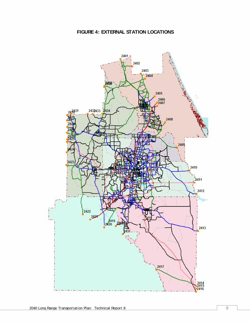
HOV for this model represents Driver plus one or more passengers (2+). The trips for each external station were derived from vehicle classification counts and surveys taken by FDOT. The results of the surveys refined the external trip travel for this model. The 2009 OUATS model contains thirty seven (37) external stations. Table 2 describes these locations and Figure 4 shows the location of the external stations. The available Florida Department of Transportation (FDOT) year 2009 traffic counts at corresponding OUATS external station locations served as the basis for the development of the external trip totals (EE plus EI trips) at each of the model’s external station TAZs. If FDOT District 5 counts were not available, then counts from surrounding FDOT Districts
Auto - External-to-Internal (EI) - Low Occupancy Vehicle (LOV)
Auto - External-to-Internal (EI) - High Occupancy Vehicle (HOV)
Auto - External-to-External (EE) - Low Occupancy Vehicle (LOV)
Auto - External-to-External (EE) - High Occupancy Vehicle (HOV)
Light Truck - External-to-Internal (EI)
Light Truck - External-to-External (EE)
Heavy Truck - External-to-Internal (EI)
Heavy Truck - External-to-External (EE)
Airport - External-to-Internal (EI) - Low Occupancy Vehicle (LOV)
Airport - External-to-Internal (EI) - High Occupancy Vehicle (HOV)
Convention Center - External-to-Internal (EI) - Low Occupancy Vehicle (LOV)
Convention Center - External-to-Internal (EI) - High Occupancy Vehicle (HOV)
Universal Orlando - External-to-Internal (EI) - Low Occupancy Vehicle (LOV)
Universal Orlando - External-to-Internal (EI) - High Occupancy Vehicle (HOV)
Sea World - External-to-Internal (EI) - Low Occupancy Vehicle (LOV)
Sea World - External-to-Internal (EI) - High Occupancy Vehicle (HOV)
Walt Disney World - External-to-Internal (EI) - Low Occupancy Vehicle (LOV)
Walt Disney World - External-to-Internal (EI) - High Occupancy Vehicle (HOV)

2040 Long Range Transportation Plan: Technical Report 8 8
were used. If FDOT counts were still not available, then counts available from county agencies were used. The counts were converted to Peak Season Weekday Average Daily Traffic (PSWADT) either by applying the Model Output Conversion Factors (MOCF) or Peak Season Conversion Factors (PSCF) to Annual Average Daily (AADT) counts and Average Daily Traffic (ADT) counts, respectively. The survey study data at the external stations was used to accurately proportion the amount of EE and EI trips to each external station of the model.
TABLE 2: EXTERNAL STATION NUMBERS AND LOCATIONS
Note: TAZ = Traffic Analysis Zone.
External Station TAZ No. Roadway and Location
External Station TAZ No. Roadway and Location
2401 U.S. 17 @ Putnam County Line 2420 U.S. 27 @ Polk Study Boundary
2402 C.R. 305 @ Flagler County Line 2421 I-4 West of S.R. 557
2403 S.R. 11 @ Flagler County Line 2422 S.R. 33 North of S.R. 559
2404 S.R. 40 @ W Volusia Study Boundary 2423 S.R. 50 @ Sumter County Line
2405 U.S. 92 @ W Volusia Study Boundary 2424 C.R. 48 @ Sumter County Line
2406 I-4 @ W Volusia Study Boundary 2425 C.R. 470 @ Sumter County Line
2407 S.R. 44 @ W Volusia Study Boundary 2426 S.R. 91 @ Sumter County Line
2408 S.R. 415 @ W Volusia Study Boundary 2427 S.R. 44 @ Sumter County Line
2409 S.R. 46 @ Volusia County Line 2428 C.R. 466A @ Sumter County Line
2410 S.R. 50 @ Brevard County Line 2429 C.R. 466 @ Sumter County Line
2411 S.R. 528 @ Brevard County Line 2430 U.S. 27 @ Marion County Line
2412 S.R. 520 @ Brevard County Line 2431 C.R. 25 @ Marion County Line
2413 U.S. 192 @ Brevard County Line 2432 C.R. 452 @ Marion County Line
2414 S.R. 60 @ Indian River County Line 2433 C.R. 450 @ Marion County Line
2415 S.R. 91 @ Indian River County Line 2434 C.R. 42 @ Marion County Line
2416 U.S. 441 @ Okeechobee County Line 2435 S.R. 19 @ Marion County Line
2417 S.R. 60 @ Polk County Line 2436 S.R. 40 @ Marion County Line
2418 C.R. 580 @ Polk Study Boundary 2437 Poinciana Parkway @ Polk Study Boundary
2419 U.S. 17-92 @ Polk Study Boundary
2040 Long Range Transportation Plan: Technical Report 8 9
FIGURE 4: EXTERNAL STATION LOCATIONS

2040 Long Range Transportation Plan: Technical Report 8 10
2.1 External Trip Development In the Year 2009 OUATS model, most of the external trips are developed within the DISTRIBUTION application with the exception of the External-External trips which are processed first in the TRIP GENERATION application using the EETRIPS_09b.dbf input file.
2.1.1 Auto External Trips Auto (no-trucks) external trips are broken down into high occupancy vehicle (HOV), and low occupancy vehicle (LOV). This break down is accomplished with the use of the EXTHOV.dbf file (in the Parameters folder) which applies the percentage of HOV trips to the auto trip table. These trips are then subtracted from the total auto external trips to obtain the LOV trips. This is done for both the EE and the EI trips.
2.1.2 Truck External Trips Truck trips at the external stations are initially determined through classification counts at the external stations to the model. These counts provide the information for breaking out light and heavy trucks. After this, these trucks are further divided by EE and EI trips based on the percentage splits of EE and EI at each external station. The result is four (4) external trip purposes at each external station. These are Light Trucks EE, Light Trucks EI, Heavy Trucks EE, and Heavy Trucks EI. A file called TRUCK.dbf (located in the Parameters folder) is used to break down these truck trips for the external stations. The file is first used to create four (4) external trip tables for the trucks, two (2) for EE and two (2) for EI. Then the file is used to develop, from the four (4) trip tables, a breakdown of Light and Heavy trucks.
2.1.3 Special Attraction External Trips The 2009 OUATS model also includes a refined external trip model for the special attractions. This is accomplished by using the data from FDOT’s non-resident travel survey done for specific special attractions in the Central Florida area. These surveys included information for determining LOV (drive alone) and HOV (driver plus one or more passengers) trips at each external station from these special attractions. The special attractions used in the OUATS model are as follows:
• Orlando International Airport (OIA) • Orange County Convention Center (OCCC). • Universal Orlando (UNI). Universal theme parks Include Universal Studios Florida and
Islands of Adventure. • Sea World (SEAW)+ • Walt Disney World (DIS). Disney theme parks include Magic Kingdom, EPCOT Center,
Disney’s Hollywood Studios, Animal Kingdom, Pleasure Island/Downtown Disney, Blizzard Beach, and Typhoon Lagoon.

2040 Long Range Transportation Plan: Technical Report 8 11
2.2 External Trip Summary After all of these external trip purposes are developed, they are converted to vehicle trips by use of auto occupancy factors, and are then combined into a special external trip table containing all of these trip purposes. For a complete breakdown, by purpose, of the external trips, both EE and EI, for the year 2009 OUATS travel demand forecasting model see Appendix Tables A-1 and A-2. The resulting trip tables for EE and EI trips get stored into two (2) files. For the EE trips, a matrix file called EETABLE_b09.mat (placed in the Scenario\Output folder) is created. A file called SPECIAL.b09 (placed in the Applications folder) contains all of the EI trip purposes combined into LOV and HOV.
3.0 TRIP GENERATION MODEL The Year 2009 OUATS model is based on the latest land use data approved by MetroPlan Orlando, updates to the year 2004 highway and transit networks, and toll data for the region’s expressways and Turnpike. This model includes all the survey information from the Florida Department of Transportation’s (FDOT) Non-Residential Travel Survey data, as well as information from the year 2000 U.S. Census. This section describes the trip generation model and the development of the internal trips. The OUATS Trip Generation Model includes the ability to vary the production and attraction rates by county. Trip interchanges within and between counties are regulated, to some extent, by the use of an input file (CTPP.dbf located in the Parameters folder) which contains inter-county and intra-county trips (Home-based Work) as determined by the Journey-to-Work (JTW) survey completed as part of the 2000 Census Transportation Planning Package (CTPP). The CTPP is a set of special tabulations from the decennial Census designed for transportation planners. CTPP contains tabulations by place of residence; place of work, and for flows between home and work.

2040 Long Range Transportation Plan: Technical Report 8 12
3.1 Trip Generation Model Overview In the Year 2009 OUATS model, the internal trips are developed within the TRIP GENRATION application. The trip generation application is the first step in the OUATS model flow chart (previously shown in Figure 3), and develops the productions and attractions, which are utilized in the trip distribution (DISTRIBUTION) application in the model chain. Trip generation estimates the total number of trips made during an average day in the peak season using traffic analysis zone (TAZ) socio-economic (SE) characteristics. The year 2009 SE data has been divided into the three (3) income level groups (High, Medium, and Low) and the data is contained in a file called ZONEDATA_09b.dbf (in the Scenario\Input folder). Please refer to Appendix Tables B-1 through B-6. The definition of zone data variables is provided in Appendix B, as well. Each trip has two (2) trip-ends, with trip productions being the home-end of the trip and trip attractions the non-home-end of the trip. This process is reversed for the special attraction trips. These trips have their productions at the special attractions, and the attraction side of the equation is the housing, hotels, and external stations. Trips that neither begin nor end at home are considered non-home based trips. Productions and attractions are defined by trip purposes. The previously used GENOUATS.exe program (written in FORTRAN) was replaced with a Voyager script based program. This was implemented as part of the 2030 LRTP model development and corresponding Year 2004 model validation. The generation model produces the following seven (7) trip purposes with variable production and attraction rates for each county:
1. Home Based Work (HBW) 2. Home Based Shopping (HBSH) 3. Home Based Social Recreation (HBSR) 4. Home Based Other (HBO) 5. Non-Home Based (NHB) 6. Truck and Taxi (TT) 7. Internal to External (IE)
Based on the efforts prepared as part of the Year 2004 model validation, the trip generation model procedure is run three (3) additional times for High, Medium, and Low income groups. In addition, a separate Truck/Taxi program calculates trucks and resultant taxi trips. This program (TRKTAXI2.exe in the User.prg folder), updates the production and attraction files from the trip generation program and produces revised production and attraction files. The output result is nine (9) trip purposes after the trucks and taxis have been separated. The following trip purposes are created for total (all) and for high (HI), Medium (ME), and Low (LO) income groups.

2040 Long Range Transportation Plan: Technical Report 8 13
1. Home Based Work (HBW) 2. Home Based Shopping (HBSH) 3. Home Based Social Recreation (HBSR) 4. Home Based Other (HBO) 5. Non-Home Based (HNB) 6. Light Truck (LT) 7. Heavy Truck (HT) 8. Taxi 9. Internal to External (IE)
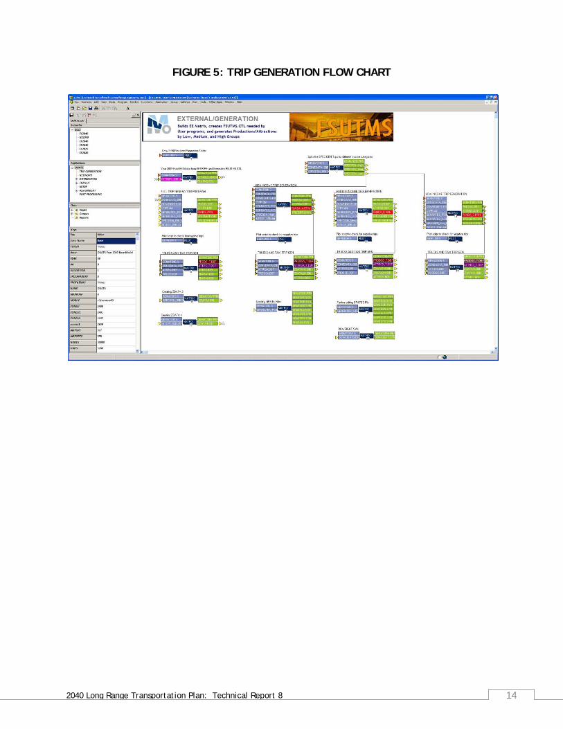
The process flow for the trip generation application is shown in Figure 5. The truck generation program is described in detail in Section 3.3.0 of this technical report. In addition to these nine (9) trip purposes, the 2009 OUATS model, with the special attraction trip purposes, includes fifteen (15) additional trip purposes to simulate travel to and from the Orlando International Airport, the Orange County Convention Center, Universal Studios theme parks, Sea World, and the Walt Disney World theme parks. The previously used executable program SPECAT15.exe has been replaced with a CUBE/Voyager script, as detailed in Section 3.2.0 of this technical report. These additional trip purposes are as follows:
1. Orlando International Airport (Tourist) 2. Orlando International Airport (Resident) 3. Orlando International Airport (EI) 4. Orange County Convention Center (Tourist) 5. Orange County Convention Center (Resident) 6. Orange County Convention Center (EI) 7. Universal Studios (Tourist) 8. Universal Studios (Resident) 9. Universal Studios (EI) 10. Sea World (Tourist) 11. Sea World (Resident) 12. Sea World (EI) 13. Walt Disney World (Tourist) 14. Walt Disney World (Resident) 15. Walt Disney World (EI)
2040 Long Range Transportation Plan: Technical Report 8 14
FIGURE 5: TRIP GENERATION FLOW CHART

2040 Long Range Transportation Plan: Technical Report 8 15
3.2 Trip Generation Model Input Data and Parameters This section describes the input data used for the Trip Generation Model, as well as, the input parameters used in this OUATS model validation effort. It also summarizes the input socioeconomic data, and the second section shows the input parameters and variables.
3.2.1 Socio-Economic Data The socio-economic (SE) data for the 2009 OUATS model validation was developed by Data Transfer Solutions (DTS) in close coordination with MetroPlan Orlando’s Land Use subcommittee. This land use data was approved by the Land Use subcommittee, the Citizens Advisory Committee (CAC), the Transportation Technical Committee (TTC), and the MPO Board and it represents the most precise data to date, derived from parcel level data and aggregated into traffic analysis zones (TAZs). The socioeconomic data summaries for each county, including regional totals, are shown in Tables 3 and 4 for productions variables and attraction variables, respectively. Appendix Figures B-1 through B-6 illustrate the TAZ boundaries applicable to the Year 2040 LRTP Update. Appendix Table B-7 provides the correlation between the previous LRTP TAZ ranges in relation to the 2040 LRTP TAZs, on a county-by-county basis.
TABLE 3: YEAR 2009 PRODUCTION VARIABLES SUMMARY
Notes: DUs denote Dwelling Units. Data reflects only the western portion of Volusia County and the northeastern part of Polk County.
Seminole Orange Osceola Lake Volusia Polk
Total DUs 113,980 299,681 92,597 130,852 78,057 29,342 744,509
Occupied DUs 106,620 283,163 78,162 113,618 73,093 22,899 677,555
Population 306,492 794,966 229,778 273,838 187,632 56,310 1,849,016
Autos 216,676 547,582 148,740 201,870 136,151 40,688 1,291,707
Total DUs 67,327 167,350 31,843 18,736 9,099 9,692 304,047
Occupied DUs 58,284 150,302 25,213 15,664 8,139 7,077 264,679
Population 113,073 328,005 58,860 39,537 15,496 14,127 569,098
Autos 95,978 225,333 39,338 21,834 10,555 12,495 405,533
Total DUs 181,307 467,031 124,440 149,588 87,156 39,034 1,048,556
Occupied DUs 164,904 433,465 103,375 129,282 81,232 29,976 942,234
Population 419,565 1,122,971 288,638 313,375 203,128 70,437 2,418,114
Autos 312,654 772,915 188,078 223,704 146,706 53,183 1,697,240
Units 3,677 89,833 33,133 2,979 1,102 3,276 134,000
Occupied Units 2,705 105,642 38,980 3,649 1,352 3,372 155,699
Occupants 5,520 215,598 79,551 7,448 2,759 6,881 317,757
Model TotalsSINGLE FAMILY
MULTI FAMILY
TOTALS
HOTEL/MOTEL
VariableCounty

2040 Long Range Transportation Plan: Technical Report 8 16
TABLE 4: YEAR 2009 ATTRACTION VARIABLES SUMMARY
Note: Data reflects only the Western portion of Volusia County and the Northeastern part of Polk County.
In addition to the SE (production and attraction variables), a special generator file (SPECGEN_09B.DBF in the Scenario\Input folder) was used. Special generators are major land use activity centers that have unique trip generation characteristics that cannot be accurately emulated using the trip rate tables or trip attraction formulas. The data included in the special generator file used in the 2009 OUATS model validation is shown in Table 5.
TABLE 5: YEAR 2009 SPECIAL GENERATORS
Note: P/A refers to the production (P) or attraction (A) and is either added (+) or subtracted (-) to or from the corresponding trip purpose (HBW, HBSH, HBSR, HBO, and NHB) total in that zone by the percentage of the designated purpose.
3.2.2 Special Attractions Socioeconomic Data The special attractions are no longer run as their own trip generation program, previously SPECAT15.exe which used the input file SPECAT15_09b.dat. The updated OUATS model setup includes script enhancements instead, which rely on SPECATR1_09b.dbf and SPECATR2_09b.dbf files stored in the Scenario\Input folder (see Appendix C-8 for printouts). The updated procedure creates production files, PRODSP1.b09 (text) and PRODSP1_B09.dbf, and attraction files ATTRSP1.b09 (text) and ATTRSP1_b09.dbf. The summary for the trip attraction files are shown in Table 6.
Seminole Orange Osceola Lake Volusia Polk
Industrial Employment 26,124 71,909 7,018 16,381 8,713 1,538 131,683
Commercial Employment 53,737 207,901 27,031 25,784 14,425 2,841 331,719
Service Employment 145,398 534,074 54,308 73,036 39,329 4,759 850,904
Employment Totals 225,259 813,884 88,357 115,201 62,467 9,138 1,314,306
School Enrollment 93,447 335,702 66,859 53,064 39,258 4,978 593,308
VariableCounty Model
TotalsSINGLE FAMILY
TAZ No. Description of Special Generator P/A
No. of Trips % HBW % HBSH % HBSR %HBO %NHB
499 University of Central Florida A+ 86,000 0 0 0 0 100630 Valencia Community College East A+ 28,700 0 0 0 0 100

2040 Long Range Transportation Plan: Technical Report 8 17
TABLE 6: YEAR 2009 SPECIAL ATTRACTION TRIP GENERATION ATTRACTIONS SUMMARY
Table 7 shows the trip production summary of the trip generation process for the special attractions based on the latest attraction survey.
3.2.3 Input Variables and Parameters This version of the OUATS model validation includes a variable trip rate, trip generation model. This program was developed specifically for the Orlando region in Voyager scripting language and allows greater flexibility for applying different trip rates to different counties based on their unique travel pattern characteristics. To validate this procedure, a target “trip table” was developed from the Center for Urban Transportation Research (CUTR) Journey-to-Work data as well as the Census Transportation Planning Package (CTPP). The Journey-to-Work data files were compiled from STF-S-5, Census of Population 1990: Number of Workers by County of Residence by County of Work. A table was created to show the county-to-county work flows using the counties in the OUATS model area. Since these work flow numbers were from the 1990 Census, they were expanded to the year 2000 based on the population from the year 2000 Census. Table 8 shows the CTPP.dbf (in the \Parameters folder) file values for year 2000 Journey-to-Work numbers. These values are used by the trip generation program as intra-county and inter-county control totals.
Trip Purpose Attraction TotalsOrlando International Airport 105,270
Orange County Convention Center 29,150
Orange County Convention Center Expansion 29,150
Universal Orlando 65,850
Sea World 37,420
Typhoon Lagoon 8,800
Pleasure Island / Downtown Disney 10,000
MGM Studios 43,500
Animal Kingdom 40,614
EPCOT Center 42,788
Blizzard Beach 9,780
Magic Kingdom 75,280

2040 Long Range Transportation Plan: Technical Report 8 18
TABLE 7: YEAR 2009 SPECIAL ATTRACTION TRIP GENERATION PRODUCTIONS SUMMARY
TAZ Special Attraction Trip Purpose PersonTourist 72,426 Resident 20,907 External-to-Internal 11,938 Tourist 10,121 Resident 8,634 External-to-Internal 10,345 Tourist 10,121 Resident 8,634 External-to-Internal 10,345 Tourist 71,945 Resident 11,751 External-to-Internal 12,154 Tourist 23,313 Resident 7,439
External-to-Internal 6,668 Tourist 7,145 Resident 886 External-to-Internal 769 Tourist 6,770 Resident 2,558 External-to-Internal 672 Tourist 40,381 Resident 1,840 External-to-Internal 1,279 Tourist 36,420 Resident 2,012 External-to-Internal 2,138 Tourist 38,620 Resident 1,985 External-to-Internal 2,182 Tourist 8,208 Resident 4,747 External-to-Internal 825 Tourist 68,339 Resident 3,960 External-to-Internal 2,981
977 Orlando International Airport
930 Orange County Convention Center Expansion
Orange County Convention Center
EPCOT Center
Blizzard Beach
928
903
899
801 Universal Orlando
931 Sea World
908 Typhoon Lagoon
902 Pleasure Island / Downtown Disney
905 MGM Studios
900 Animal Kingdom
897 Magic Kingdom

2040 Long Range Transportation Plan: Technical Report 8 19
TABLE 8: YEAR 2000 CTPP JOURNEY-TO-WORK TRIPS
Notes: (1) = Journey-to-Work (JTW) from year 2000 CTPP. * = Only the west side of Volusia County and a small northeast portion of Polk County. Since the Census information only dealt with the Home-Based Work Trip (HBW), the factors that were applied to Home-Based Work were also applied to Home-Based Shopping (HBSH), Home-Based Social-Recreation (HBSR), Home-Based Other (HBO), and the Non-Home-Based (NHB), trip purposes to maintain the inter-county relationships. The input parameter files needed for this variable trip production and attraction rate model are the GENRATES_P.dbf (productions rates) and GENRATES_A.dbf (attraction rates). Both files need to be located in the Parameters folder. The Voyager scripting uses the two (2) files to develop seven (7) text files that are used by the MODE CHOICE program (in FORTRAN) in later steps. The seven (7) files created (in the Applications folder) are named:
1. GRATESE.SYN (for Seminole County) 2. GRATEOR.SYN (for Orange County) 3. GRATEOS.SYN (for Osceola County) 4. GRATELA.SYN (for Lake County) 5. GRATEVO.SYN (for Volusia County) 6. GRATEPO.SYN (for Polk County) 7. GRATES.SYN
The OUATS Trip Generation Model also uses a dwelling unit occupancy distribution input file (DUWEIGHTS.dbf located in the Parameters folder) which is used to disaggregate the dwelling unit distribution based on household occupancy rates and persons-per-household. This file is summarized as shown in Appendix Table C-1. The final validated production and attraction rates for each county are provided in Appendix Tables C-2 through C-7.
County (Origin/Destination) Seminole Orange Osceola Lake Volusia* Polk* Other TotalsSeminole 127,110 113,990 1,876 1,160 1,928 189 6,998 253,251
Orange 36,599 512,554 10,456 2,734 1,083 688 12,557 576,671
Osceola 1,087 31,472 42,325 101 40 436 2,051 77,512
Lake 2,243 13,748 660 65,487 1,811 201 3,623 87,773
Volusia* 13,927 10,841 237 568 34,430 61 2,010 62,074
Polk* 57 2,214 1,162 92 0 604 0 4,129
Other 5,510 30,285 5,366 8,741 6,382 0 0 56,284
Totals 186,532 715,104 62,082 78,884 45,673 2,181 27,239 1,117,695

2040 Long Range Transportation Plan: Technical Report 8 20
3.3 Truck Generation Program The truck trip generation program used in this model validation, as in the year 2004 model validation efforts, is based on procedures developed for the Greater Vancouver (British Columbia, Canada) Regional District (GVRD) truck model. That model was developed to estimate 24-hour light and heavy truck travel demand for current and future years. Light trucks are classified as having a gross vehicle weight (GVW) of 4,500-20,000 kilograms (kg). Trucks over 20,000 kg are classified as heavy trucks. The Federal Highway Association (FHWA) vehicle classification types 5 through 7 represent light trucks and 8 through 13 represent heavy trucks. Each weight class has different trip generation and distribution characteristics as described below. The trip generation for this process estimates the number of truck trips produced and attracted by each traffic zone based on population, wholesale, manufacturing, and non-wholesale employment for that zone. The trip generation equations for light and heavy trucks are as follows:
Light Truck (Productions/Attractions) = (0.018 * Total Population) + (0.528 * Commercial Employment) + (0.0373 * Industrial and Service Employment)
Heavy Truck (Productions/Attractions) = (0.287 * Commercial Employment) + (0.116 * Industrial Employment)
3.4 Special Attractions Program An improved process was developed for the year 2000 OUATS model validation effort for special attractions. The additional purposes provided a better model validation, as well as the capability to analyze trips separately going to and from the airport as well as the major area theme parks. This program was revised and updated during the 2000 modeling effort to include additional attractions and to include a detailed external station analysis. This information was derived from the non-resident surveys conducted by FDOT. The revised program (SPECAT15.exe) has since been replaced as part of the year 2009 validation effort as mentioned in Section 3.2.2 of this report. The program now uses a set of database input files (SPECATR1_09b.dbf and SPECATR2_09b.dbf) that are processed in the script setup.
3.4.1 Special Trip Generation Methodology The development of internal productions and attractions for the special trip purposes, Orlando International Airport, Orange County Convention Center, Universal Orlando, Sea World, Typhoon Lagoon, Pleasure Island/Downtown Disney, Disney/MGM Studios, Animal Kingdom, EPCOT Center, Blizzard Beach, and the Magic Kingdom, are now included in the Model’s script and uses the input files, SPECATR1_09b.dbf and SPECATR2_09b.dbf (located in Scenario\Input folder) that is part of the DISTRIBUTION application. The file is also used for the development of EI trips for the special attractions.

2040 Long Range Transportation Plan: Technical Report 8 21
3.4.2 Special Attractions Program Summary The output of the special attractions trip generation process is the development of the person trip production file PRODSP1_b09.dbf and the person trip attraction file ATTRSP1_b09.dbf. Both files contain fifteen (15) trip purposes. These trip purposes are shown in Table 9 and the results of this program have been shown previously in Tables 6 and 7. TABLE 9: SPECIAL ATTRACTIONS PRODUCTIONS AND ATTRACTIONS TRIP PURPOSES
3.5 Trip Generation Results After the trip generation program and truck trip generation program (TRKTAXI2.exe) is run, a nine (9) purpose attractions file (ATTRS_T.dbf) and a nine (9) purpose productions file (PRODS_T.dbf) are produced which are used as input to the TRIP DISTRIBUTION application. The process is repeated three (3) times for the High (ATTRSA_T.dbf and PRODSA_T.dbf), Medium (ATTRSB_T.dbf and PRODSB_T.dbf), and Low (ATTRSC_T.dbf and PRODSC_T.dbf) data variables from the ZONEDATA_09b.dbf. Table 10 shows the resultant productions and attractions, summarized by county and totaled for the region, which are output from the TRIP GENERATION application. In addition, various Trip Generation statistics are included and are shown in Table 11.
PRODSP1 & ATTRSP1 Trip PurposeOrlando International Airport – Tourist
Orlando International Airport – Resident
Orlando International Airport – EI
Orange County Convention Center - Tourist
Orange County Convention Center - Resident
Orange County Convention Center - EI
Universal Orlando – Tourist
Universal Orlando – Resident
Universal Orlando – EI
Sea World - Tourist
Sea World - ResidentSea World - EIDisney - TouristDisney - ResidentDisney - EI

2040 Long Range Transportation Plan: Technical Report 8 22
TABLE 10: YEAR 2009 TRIP GENERATION MODEL OUTPUT
Note: (1) Percentages shown are of total model productions.
(2) Percentages shown are of total model attractions.
TABLE 11: YEAR 2009 TRIP GENERATION STATISTICS
Seminole 141,178 114,341 72,598 236,452 403,128 44,734 18,455 85,895 N/A
Orange 395,098 386,305 307,018 745,352 1,742,275 161,896 68,009 269,214 N/A
Osceola 180,343 186,809 157,251 368,895 278,535 22,968 8,568 80,943 N/A
Lake 103,441 87,399 58,243 174,554 215,933 23,582 9,298 62,107 N/A
Volusia 75,544 61,668 39,996 129,084 119,297 13,705 5,157 34,978 N/A
Polk 14,271 12,457 8,735 23,545 11,632 3,129 995 3,040 N/A
Externals N/A N/A N/A N/A N/A N/A N/A N/A 393,471
Totals 909,875 848,979 643,841 1,677,882 2,770,800 270,014 110,482 536,177 393,471
% (1) 11.15% 10.40% 7.89% 20.56% 33.95% 3.31% 1.35% 6.57% 4.82%
Seminole 151,371 132,894 104,842 267,995 403,128 44,734 18,455 85,895 30,916
Orange 546,930 513,297 366,090 960,556 1,742,275 161,896 68,009 269,214 93,841
Osceola 89,406 100,163 74,589 208,287 278,535 22,968 8,568 80,943 43,700
Lake 77,408 63,762 60,707 145,477 215,933 23,582 9,298 62,107 106,941
Volusia 41,977 35,657 33,812 88,528 119,297 13,705 5,157 34,978 84,140
Polk 2,788 3,179 3,797 7,069 11,632 3,129 995 3,040 33,949
Externals - - - - - - - - -
Totals 909,880 848,952 643,837 1,677,912 2,770,800 270,014 110,482 536,177 393,487
% (2) 11.15% 10.40% 7.89% 20.56% 33.95% 3.31% 1.35% 6.57% 4.82%
PRODUCTIONS
ATTRACTIONS
HBO NHBLIGHT TRK
HEAVY TRK TAXI EICounty HBW HBSH HBSR
Seminole Orange Osceola Lake Volusia PolkTotal Permanent Population 419,565 1,122,971 288,638 304,376 203,128 70,437 2,409,115
Total Population (Permanent + Transient) 428,534 1,363,346 408,497 335,216 211,952 87,917 2,835,463
Total Permanently Occupied Dwelling Units 164,905 433,467 103,375 129,282 81,232 29,977 942,238
Total Occupied (Permanent + Transient ) Dwelling 170,170 532,169 150,386 142,650 84,798 38,086 1,118,259
Total Employment 225,259 813,884 88,357 115,201 62,467 9,138 1,314,306
Total Service Employment 145,398 534,074 54,308 73,036 39,329 4,759 850,904
Permanent Population per Permanently Occupied 2.54 2.59 2.79 2.35 2.50 2.35 2.56
Total Population per Total Occupied dwelling Unit 2.52 2.56 2.72 2.35 2.50 2.31 2.54
Total Service Employment per Total Population 0.65 0.66 0.61 0.63 0.63 0.52 0.65
Total Home-Based Productions (Person Trip Ends) 564,569 1,833,773 893,298 423,637 306,292 59,008 4,080,577
Total Home-Based Attractions (Person Trip Ends) 657,102 2,386,873 472,445 348,354 199,974 16,833 4,081,581
Total Productions 1,114,446 4,061,472 1,284,020 733,990 477,726 77,540 7,749,194
Total Attractions 1,237,895 4,708,413 906,867 764,648 455,548 69,314 8,142,685
Total Trips per Permanently Occupied Dwelling Units 6.76 9.37 12.42 5.68 5.88 2.59 8.22
Total Trips per Total Occupied Dwelling Units 6.55 7.63 8.54 5.15 5.63 2.04 6.93
Total Trips per Employment 4.95 4.99 14.53 6.37 7.65 8.49 5.90
County Model TotalsStatistics

2040 Long Range Transportation Plan: Technical Report 8 23
Note: Volusia and Polk Counties are based on partial data for area in the model.
4.0 TRIP DISTRIBUTION MODEL This section describes the gravity model and input data used for the OUATS year 2009 Trip Distribution model. This Trip Distribution model creates person trips, runs a default mode split model, and then runs an initial highway assignment to obtain restrained highway skim times for the transit network. This section describes the gravity model’s methodology and operation, as well as the input variables and parameters used.
4.1 Trip Distribution Model Overview The trip distribution step is the third application in the OUATS model chain (refer to Figure 3) and develops the person trip tables, which are used throughout the rest of the model chain. Trip distribution estimates the flow of traffic between all trip origins and destinations at the traffic analysis zone level.
The distribution model uses this information:
The number of productions and attractions for each internal and external zone; Travel impedances, such as travel time, terminal time, and travel cost, and; Trip length frequencies (reflected in friction factors).
FSUTMS uses a gravity model formulation (based on Sir Isaac Newton’s Law of Gravity) for the distribution of trips by purpose. Trips are distributed between zones based on the number of productions and attractions generated at each zone and the travel impedances between the zones. A more detailed illustration of the TRIP DISTRIBUTION application’s inputs and outputs is shown in Figure 6.
FIGURE 6: TRIP DISTRIBUTION FLOW CHART

2040 Long Range Transportation Plan: Technical Report 8 24
4.2 Gravity Model Methodology and Operation The crucial part of this application is the gravity model. The gravity model accepts zonal trip end productions and attractions stratified by class of trip (purpose, geography, time of day, etc.), travel impedance factors, zone-to-zone travel indices, and generates a zone-to-zone trip table (matrix) file from the Gravity Model distribution formula. The model also checks the acceptability of computed attractions, and if necessary, adjusts the calculated attractions to each zone to equal the sum of the input productions for the area. The Gravity Model originally paralleled Newton’s gravitational law. The premise is that all trips starting from a given zone are attracted by various traffic generators in other zones and that this attraction is directly proportional to the relative attraction of the zone and inversely proportional to the separation between the zones in the gravity model. The measure of separation is generally accepted as the zone-to-zone travel time via the specified transportation network. However, because people as social beings do not order their lives according to exact physical laws, an adjustment was necessary to modify the gravitational concept to fit the travel characteristics of the urban area being studied. The classical gravitational formula is:
2040 Long Range Transportation Plan: Technical Report 8 25
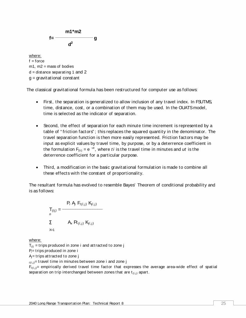
m1*m2 f= ____________________ g d2 where:
f = force m1, m2 = mass of bodies
d = distance separating 1 and 2 g = gravitational constant
The classical gravitational formula has been restructured for computer use as follows:
• First, the separation is generalized to allow inclusion of any travel index. In FSUTMS, time, distance, cost, or a combination of them may be used. In the OUATS model, time is selected as the indicator of separation.
• Second, the effect of separation for each minute time increment is represented by a table of “friction factors”; this replaces the squared quantity in the denominator. The travel separation function is then more easily represented. Friction factors may be input as explicit values by travel time, by purpose, or by a deterrence coefficient in the formulation F(ti) = e -ut, where ti is the travel time in minutes and ut is the deterrence coefficient for a particular purpose.
• Third, a modification in the basic gravitational formulation is made to combine all these effects with the constant of proportionality.
The resultant formula has evolved to resemble Bayes’ Theorem of conditional probability and is as follows: Pi Aj Ft(i,j) K(i,j) T(ij) = ________________________ n ∑ Ax Ft(i,j) K(i,j) X=1 where:
T(ij = trips produced in zone i and attracted to zone j Pi= trips produced in zone i Aj= trips attracted to zone j t(i,j)= travel time in minutes between zone i and zone j
Ft(i,j)= empirically derived travel time factor that expresses the average area-wide effect of spatial separation on trip interchanged between zones that are t(i,j) apart.

2040 Long Range Transportation Plan: Technical Report 8 26
K(i,j)= specific zone-to-zone adjustment factor to allow for the incorporation of the effect on travel patterns of defined social or economic linkages not otherwise accounted for in the gravity model formulation. Therefore, in the OUATS FSUTMS gravity models, to balance the attractions, the number of iterations and the convergence criteria are specified and the model iterates until either convergence or the number of iterations specified by the user is met. Attraction iterations are based on individual zonal level adjustments.
4.3 Gravity Model Inputs and Variables There are four (4) essential inputs to the DISTRIBUTION module:
• A zone-to-zone travel impedance matrix (FHSKIMS.ayy and FHSKIMS2.ayy files) • Terminal times (included in Keys area and in PROFILE.mas file) • Trip productions (PRODS_T.dbf, and PRODSP1_b09.dbf) and trip attractions (ATTRS_T.dbf
and ATTRSP1_b09.dbf) • Friction factors (FF.dbf, FFSA1.dbf, and FFSA2.dbf)
4.4 Special Trips Development The additional fifteen (15) purposes in the 2009 OUATS Trip Distribution Model have been updated using the non-residential travel survey conducted by FDOT in 2001. Section 4.4.1 discusses how the special purpose external-to-internal trips (EI) are developed, followed by section 4.4.2 which deals with the internal trips (Tourist and Resident).
4.4.1 Special External Trip Development The development of external-internal trips for the special trip purposes (Airport, OCCC, Universal, Sea World, and Disney), occurs in both the external trip module (for HOV calculation) and in the trip distribution module, which combines the LOV and HOV special trip purposes into a multi-purpose trip table. The external trips for the special purposes are developed in the trip distribution module of the FSUTMS model chain. The procedure was originally developed as part of the 2000 model validation effort and is updated as part of the effort for 2009. These external trips were taken directly from attraction surveys conducted by FDOT in 2001. The special attraction files are used to provide the number of person trips for each special attraction (by each traffic analysis zone). The production end is based on the “capacity target” of the special attraction. For example, the number of passenger enplanements per day is used as the restriction for the OIA. The number is then split into production (file PRODSP1_b09.dbf) and attraction (file ATTRSP1_b09.dbf) purposes (tourist, residential, and external-internal) by the percentages

2040 Long Range Transportation Plan: Technical Report 8 27
provided in the SPECATR1_09b.dbf and the SPECATR2_09b.dbf files and distributed based on the procedure described previously. The procedure to develop these trips starts by extracting the external trip tables for the Orlando International Airport (APT EI), the Orange County Convention Center (OCCC-EI), Universal Orlando (UNI-EI), Sea World (SEAW-EI), and Disney World (DIS-EI) from the twenty four (24) purpose person trips file, PTRIPS.mat (purposes 12,15,18,21, and 24 respectively). Auto occupancy factors are then applied to convert to vehicle trips and the vehicle trips from the external trip module (EETABLE_b09.mat) are then added to obtain total vehicle trips from the external stations. Once the total external number of trips has been determined, the next step is to separate LOV and HOV external trips. An input file (EXTHOV.dbf in the Parameters folder) contains the percentage of external trips (both EI and EE) that are HOV. These trips are then extracted from the total trips at the external stations to develop separate LOV and HOV trip tables for the external stations. This process also includes the steps to split out the LOV and HOV EE and EI auto trips and the EE and EI light and heavy truck trips. The resultant trip table (SPECIAL.b09) is then used in subsequent highway trip table development for input into the preliminary highway assignment.
4.4.2 Special Internal Trip Development The internal trips for the special purposes are handled separately from the other trip purposes for their inclusion into the default mode split model in the trip distribution process. These ten (10) trip purposes are extracted and re-ordered so that each pair has the resident sub-purpose first. This allows the usage of the home based other/non-home based logit in the mode choice model. The output matrix located in applications files for inclusion into the mode choice model are SPECPORG.mat and SPECPURP.mat (each file is also created in binary format with extension *.tem for the program to read). During the default modal choice model, two (2) vehicle trip table files are produced for the nine (9) original purposes for the work trip (HTWRKDEF.b09) and for the non-work trip (HTNWKDEF.b09). These two (2) files have both LOV and HOV trip tables. Additionally, the special purpose files (SPECPORG.tem and SPECPURP.tem) have auto occupancy factors applied to them for inclusion into the highway trip table for the initial highway assignment to obtain restrained travel times for the transit network. Subsequent processing of these special internal trip purposes develops both LOV and HOV trip tables. Files are created and then combined to obtain an initial highway trip table (HTTABFD.mat) which has both LOV and HOV trip purposes, for use in the preliminary highway assignment process.

2040 Long Range Transportation Plan: Technical Report 8 28
4.5 Trip Distribution Results One of the output files from the trip distribution module is a person trip (PTRIPS.mat) file which results from the processing of four (4) gravity models. Important statistics, including total person trips, intra-zonal trips, and average trip lengths, are shown in Table 12.
TABLE 12: DAILY TRIP DISTRIBUTION SUMMARY
5.0 MODE CHOICE MODEL The mode choice model determines the amount of travel that will take place on each available mode of transportation. Separate models are used for the three main trip purposes (HBW, HBNW and NHB). This is because people have different propensities for using transit for different types of trips. For example, people are more willing to use transit for work trips than for other trips. In addition, separate models are used to estimate mode choice by automobile as a surrogate measure of income. The mode choice step is the fifth step in the OUATS model chain, and is a recalibrated version of the 2004 OUATS mode choice model. The 2004 OUATS mode choice model contains 11 steps, three for HBW, one for HBNW, one for NHB
Average TripTotal Trips Trips % of Total Length (min)
HBW 909,875 26,401 2.9 23.07
HBNW / HBSH 848,979 203,248 23.9 14.86
HBSR 643,841 120,121 18.7 16.54
HBO 1,677,882 388,720 23.2 15.41
HBNW Total 3,170,702 712,089 22.5 N/A
NHB 2,770,800 289,557 10.5 16.31
Subtotals 6,851,377 1,028,047 15.0 N/ALight Truck 270,014 42,399 15.7 15.52
Heavy Truck 110,482 19,885 18.0 14.70
Taxi 536,177 83,872 15.6 16.69
EI 393,471 N/A N/A 34.93
APT (TOUR) 72,426 210 0.3 28.52
APT (RES) 20,907 0 0.0 36.97
APT (EI) 11,938 0 0.0 49.41
APT Total 105,271 210 0.2 N/A
OCCC (TOUR) 20,242 185 0.9 15.21
OCCC (RES) 17,368 0 0.0 31.16
OCCC (EI) 20,690 0 0.0 53.93
OCCC Total 58,300 185 0.3 N/A
UNI (TOUR) 71,945 1,121 1.6 16.58
UNI (RES) 11,752 0 0.0 28.71
UNI (EI) 12,154 0 0.0 50.73
UNI Total 95,851 1,121 1.2 N/A
SEAW (TOUR) 23,312 442 1.9 14.03
SEAW (RES) 7,439 4 0.1 29.55
SEAW (EI) 6,668 0 0.0 52.00
SEAW Total 37,419 446 1.2 N/A
DIS (TOUR) 205,883 11,139 5.4 19.59
DIS (RES) 13,989 0 0.0 38.88
DIS (EI) 10,845 0 0.0 56.00
DIS Total 230,717 11,139 4.8 N/A
ALL PURPOSES Total 9,216,637 1,200,405 13.0 N/A
Trip PurposeIntrazonal Trips
STANDARD PURPOSES
SPECIAL PURPOSES

2040 Long Range Transportation Plan: Technical Report 8 29
and one each for the Orlando International Airport, the Universal Studios theme parks, the Walt Disney World theme parks, the Orange County Convention Center, International Drive, and the Sea World theme park. As before, the HBW trips have been divided into three income markets (high, medium and low). This section describes the methodologies used and the operation of the 2009 OUATS mode choice model (see Figure 7).
FIGURE 7: MODE FLOW CHART
During this process, person trip tables are subdivided by the mode choice model into the following modes:
1. Single-occupant auto (Low Occupant Vehicle, or LOV) 2. Two or more occupant auto (High Occupant Vehicle, or HOV); 3. Local bus 4. Transit (light rail, fixed guideway, express bus, etc.).
The OUATS mode choice model is structured in a nested logit form. The nested structure allows for submodal trade offs to be fairly sensitive to service measures while lessening the impact on other less related sub-modes. This nesting structure is shown in Figure 8.

2040 Long Range Transportation Plan: Technical Report 8 30
FIGURE 8: OUATS MODE CHOICE NESTING STRUCTURE
The degree of sensitivity of each nest is measured by the magnitude of its nesting coefficient. The nesting coefficient varies between zero to one. If the nesting coefficient is one then the nesting logit model structure becomes identical to multinomial logit model form. The closer a nesting coefficient is to zero the more elastic that particular nest would become. The most salient features of this nested logit structure are:
• Separation of auto submodes by vehicle occupancy; i.e., drive alone and shared ride.
The shared ride category is further subdivided into auto with two occupants and auto with three-or-more occupants.
• Separation of auto access transit trips by park-and-ride (PNR) and kiss-and-ride (KNR)
to reflect the kiss-and-ride market within the study area and the need to estimate mode-of-arrival at transit stations.
In the primary nest of the 4-level nested structure, total person trips are divided into “Auto” and “Transit” trips. In the secondary nest, the auto trips are split into “Drive Alone” and “Shared Ride” trips, and the transit trips are split into “Walk Access” and “Auto Access (Premium)” trips. In the third nest, shared ride trips are further divided into “One Passenger (SR2)” and “2+ Passengers (SR3+)”. On the transit side in this third nest, the walk access trips are split into “Local Bus” and “Premium Modes” trips, and the auto access trips are divided into “Park-N-Ride” and “Kiss-N-Ride” trips. In the fourth nest, premium transit trips, if needed, can be further divided into Express Bus, BRT, LRT, and Commuter Rail.

2040 Long Range Transportation Plan: Technical Report 8 31
The nesting structure assumes that the elasticity or sensitivity to travel characteristics will be greater at the lower levels of the nest. The sensitivity of each mode is estimated using a nesting coefficient in a range of zero to one. It is inversely proportional to the sequential product of all nesting coefficients of the upper level nests including the current level. Thus, a choice between premium and local transit, for example, at a lower level of the nest, would be quite sensitive to the competition between these submodes. The impact of a change in one submode would be diminished at a higher level of decision (on main mode choice between transit and auto, for example). The mode choice model operates for 11 trip purposes: three home based work (HBW), home based non-work (HBNW), non-home based (NHB), Disney (DIS), Universal (UNI), Airport (MCO), Orange County Convention Center (OCC), International Drive (I-Drive) and Sea World (SEW).
5.1 Default Mode Choice Model The default mode choice model, which is run prior to the initial highway assignment, estimates initial auto occupancies to allocate trips between LOV and HOV categories. Unlike the final mode choice model, which includes the additional special purposes, the default mode choice model operates for only three trip purposes: home based work, home based non-work, and non-home based. The analysis is performed using default transit splits with work and non-work auto occupancies estimated using unconstrained highway speeds. The regional mode splits for the default mode choice model are as follows: Home Based Work 1.30 % Home Based Non-Work 0.40 % Non-Home Based 0.20 %
The default mode choice model is designed to develop a reasonable, preliminary allocation between LOV and HOV for the initial equilibrium assignment and capacity-restrained speed determination. The initial highway assignment produces a “loaded” highway network (HRLDXY.TEM) from which the congested highway impedance skims are developed (RHSKIMS.ayy for LOV, and RHSKIMS2.ayy for HOV). The congested skims allow the mode choice model to accurately estimate shifts between available modes in the peak period.
5.2 Mode Choice Model Operation For the purposes of the Orlando Urban Area Transportation Study, the mode choice model has been divided into 10 parts, three work mode choice models, a non-work mode choice model, and six special purposes; Disney World, Universal Studios, Orlando International Airport, Orange County Convention Center, International Drive and Sea World. These six additional special purposes are run as separate applications of the mode choice model. There are actually 10 purposes, with resident and tourist purposes for each of the six special purposes. Each pair is treated the same way as the HBNW/NHB application of the model, with the resident purpose using the same logic as HBNW and the tourist purpose using the NHB logic.

2040 Long Range Transportation Plan: Technical Report 8 32
The mode choice model assumes that work trips occur in the peak period and are subject to congested travel conditions, and non-work trips occur in the off-peak period and are subject to uncongested travel conditions. Therefore, the work mode choice model uses the congested impedance skims where the non-work mode choice model uses the free-flow impedance skims. Congested travel times are estimated by a default mode choice and an initial highway assignment in the Trip Distribution Step of the model chain. The default mode choice model is a simplified version of the final mode choice model. It uses reasonable, accurate assumptions of estimated modal shifts. The vehicle trip tables created by the default mode choice model are assigned to the highway network. The loaded network is then “skimmed” to create a congested travel time matrix used by the mode choice model. Although the 2000 OUATS model network has no high occupancy vehicle (HOV) facilities (because of the lack of enforcement, the HOV lanes currently designated on I-4 are effectively used as general purpose lanes), the model is structured so that the estimation of highway trips by auto occupancy category is sensitive to different impedances from LOV and HOV networks. Thus, the model is capable of responding to relative differences in LOV and HOV network performances and has the ability to shift trips from one mode to another. HOV skims are developed by the model; however, because there are no coded HOV facilities in the 2009 network, the HOV skims are equal to non-HOV skims in 2004. The OUATS mode choice model’s calibrated coefficients were based on the 2009 LYNX bus ridership results.
5.3 Mode Choice Special Purposes As indicated in section 5.2, additional consideration and treatment is given to the special purposes added as part of the 2004 OUATS model validation. These special purposes, for the mode choice operation, are as follows: Disney Resident Disney Non-Resident Universal Resident Universal Non-Resident Airport Resident Airport Non-Resident Convention Center Resident Convention Center Non-Resident International Drive Resident International Drive Non-Resident Sea World Resident Sea World Non-Resident
These purposes, as used in the revised modal choice program (MODEORL5.EXE), and are triggered by a new version option in the PROFILE.MAS (the &VERS parameter, which is set to six for Orlando Special Purposes), and by six new “code” flags at the mode choice program

2040 Long Range Transportation Plan: Technical Report 8 33
execution time (DIS, UNI, MCO, OCC, and SEW). This means that the mode choice program (MODEORL5.EXE) is executed 11 times in the PILOT script of the mode choice step. An additional feature of this program is the use of individual mode split coefficient files for home based work, non-work and special purposes. MODE_H.SYN – High income work trip modal coefficients MODE_M.SYN – Medium income work trip modal coefficients MODE_L.SYN – Low income work trip modal coefficients MODE_NW.SYN – Non-work trip modal coefficients MODE9IDR.SYN – I-Drive modal coefficients MODE9DIS.SYN - Disney modal coefficients MODE9UNI.SYN - Universal modal coefficients MODE9MCO.SYN - Airport modal coefficients MODE9OCC.SYN – Orange County Convention Center modal coefficients MODE9IDT.SYN – International Drive modal coefficients MODE9SEW.SYN - Sea World modal coefficients
5.4 Changes to the Mode Choice Program The changes made for the 2004 OUATS mode choice model were continued for 2009.
These changes are explained here for easy reference. These features make the mode choice program compatible with the current FSUTMS transit framework. The mode choice FORTRAN program is called MODEORL5.EXE, and correspondingly the source code is called MODEORL5.FOR. The FORTRAN code was compiled using Intel’s FORTRAN compiler. Important features of MODEORL5.EXE are:
The PCWALK file contains a single walk area of 1/2 mile. It computes mode shares across three access categories (can walk, must drive and no access). The code reads the streamlined percent walk data (PCWALK), correctly executes computations across the three access categories, and reports trips from those categories. This procedure replaces the short-/long- walk methodology. Short-walk was defined as 1/3 of a mile and long-walk had a range up to one mile.
The AUTOCON program incorporates all station-specific information on the connector, which was done originally to accommodate multi-pathing. In addition, all information on the connector is weighted to in-vehicle time. Mimicking the same functionality, many existing mode choice models perform a transit station lookup to apply the station-specific information (e.g., station parking cost and access time) to the utility equation for auto-access utilities. These models also determine the auto operating cost for the trip using the highway skims.
All code related to adding station-specific data to the utilities was commented out;

2040 Long Range Transportation Plan: Technical Report 8 34
The station parking costs on the auto-access connector reflect standard HBW and HBO calculations, which means they are divided by two to reflect half of the trip. These costs are typically full value for NHB trips, which may not have a "return" leg. The other half of the parking costs was added to the disutility for NHB trips.
Since separate KNR connectors are not required as part of the current framework, an adjustment to the weighted station access time was made for KNR utilities.
The current FSUTMS transit framework specifies mode choice structures and coefficients. The path weights in the transit path building were made consistent with the mode choice coefficients.
Tables for general input values for the 11 purposes in the mode choice model and specific trip purpose input parameters are shown in Appendix D-1 for the Mode Choice Model.
5.5 Mode Choice Output The output data from the OUATS mode choice model consists of two components, highway trips and transit trips. The highway trips consist of three components: Drive Alone One Passenger Two+ Passengers
While the transit trips consist of four components: Walk to local Walk to premium Park and Ride Kiss and Ride
All seven of these components are determined by the mode choice program for the following 15 trip purposes: Home Based Work HBWRK Home Based Non-Work HBNWK Non-Home Based NHB Disney Resident DIS RES Disney Non-Resident DIS NR Universal Resident UNI RES Universal Non-Resident UNI NR Airport Resident MCO RES

2040 Long Range Transportation Plan: Technical Report 8 35
Airport Non-Resident MCO NR Convention Center Resident OCC RES Convention Center Non-Resident OCC NR I-Drive Resident I-Drive Non-Resident Sea World Resident SEW RES Sea World Non-Resident SEW NR
The summary results of the mode choice model for the 2000 OUATS model validation for these 15 mode choice purposes are shown in Appendix E– “Mode Choice Model” and the final Total Mode Choice Output is shown below in Table 13.
TABLE 13: TOTAL MODE CHOICE OUTPUT
Person Drive One Two+ Walk to Walk to Park- Kiss-
Trips Alone Passenger Passenger Local Premium Ride Ride Total
Zero Car Households 135,204 56,153 39,003 31,521 7,098 66 441 922 8,527
One Car Households 3,065,798 1,274,732 894,637 877,924 15,788 91 1,422 1,204 18,505
Two+ Car Households 4,055,551 2,178,652 1,284,993 575,100 12,984 34 2,213 1,575 16,806
Total 7,256,552 3,509,536 2,218,633 1,484,545 35,869 192 4,076 3,701 43,838
Can Walk 2,034,388 926,770 637,451 431,892 35,869 192 900 1,314 38,275
Must Drive 1,779,159 799,260 503,608 470,728 - - 3,176 2,387 5,563
No Access 3,443,005 1,783,506 1,077,574 581,925 - - - - -
Total 7,256,552 3,509,536 2,218,633 1,484,545 35,869 192 4,076 3,701 43,838
Productions:
CBD 128,578 63,246 38,492 22,179 4,635 9 5 11 4,661
Exurban 3,716,562 1,795,491 1,139,185 766,584 9,901 60 2,637 2,704 15,302
Other 3,411,412 1,650,799 1,040,956 695,783 21,333 123 1,434 985 23,874
Attractions:
CBD 245,348 113,723 70,403 49,452 9,832 14 867 1,057 11,769
Exurban 3,119,662 1,599,253 994,679 514,894 8,844 45 972 977 10,837
Other 3,891,542 1,796,560 1,153,551 920,200 17,194 133 2,237 1,667 21,231
Total 7,256,552 3,509,536 2,218,633 1,484,545 35,869 192 4,076 3,701 43,838
Highway Trips Transit Trips
2040 Long Range Transportation Plan: Technical Report 8 36
6.0 HIGHWAY ASSIGNMENT AND EVALUATION MODELS The Year 2009 OUATS model is based on the latest land use data approved by MetroPlan Orlando, updates to the year 2004 highway and transit networks, and toll data for the region’s expressways and Turnpike. This model also includes all of the survey information from the Florida Department of Transportation’s (FDOT) Non-Residential Travel Survey data as well as information from the year 2000 Census. This section shows the results of the highway assignment and evaluation.
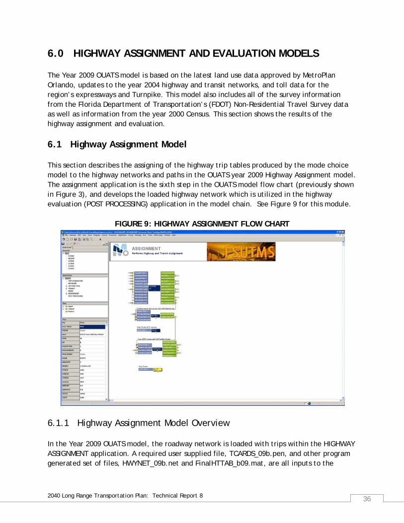
6.1 Highway Assignment Model This section describes the assigning of the highway trip tables produced by the mode choice model to the highway networks and paths in the OUATS year 2009 Highway Assignment model. The assignment application is the sixth step in the OUATS model flow chart (previously shown in Figure 3), and develops the loaded highway network which is utilized in the highway evaluation (POST PROCESSING) application in the model chain. See Figure 9 for this module.
FIGURE 9: HIGHWAY ASSIGNMENT FLOW CHART
6.1.1 Highway Assignment Model Overview In the Year 2009 OUATS model, the roadway network is loaded with trips within the HIGHWAY ASSIGNMENT application. A required user supplied file, TCARDS_09b.pen, and other program generated set of files, HWYNET_09b.net and FinalHTTAB_b09.mat, are all inputs to the

2040 Long Range Transportation Plan: Technical Report 8 37
HIGHWAY PROGRAM (step 3) of this application. The output of the highway assignment includes the loaded highway network file, HRLDXY_b09.net. Figure 9 shows the various files.
6.1.2 Highway Assignment Model Methodology and Operation The highway assignment application utilizes the output from the NETWORK application (HWYNET_09b.net) as well as the MODE CHOICE application (HTTAB_b09.mat). The HTTAB_b09.mat is combined with the AMTransitAUTO.mat file and the MDTransitAuto.mat file from the TASSIGN sub-application to form a total highway trip table called FinalHTTAB_b09.mat. This total highway trip table is then assigned to the highway network, HWYNET_09b.net, and TCARDS_09b.pen file. The TCARDS_09b.pen is a user supplied input file that includes turn penalties as well as time penalties. Time penalty locations are depicted in Figure 10. The output of the highway assignment application includes a “loaded” highway network entitled HRLDXY_b09.net. This file is generated after several iterations of capacity restraint assignments are made using this equilibrium assignment technique. Results of the output are explained further in the following section.
6.2 Highway Assignment Results The output from the highway assignment module is a loaded network (HRLDXY_b09.net) file. Important attributes from the loaded highway file include capacity, time, speed, vehicle distance traveled, vehicle hours traveled, and volume. The loaded network file is used as an input for the HIGHWAY EVALUATION application to generate more results as well as statistics to further explain and validate the OUATS year 2009 Model.
6.3 Highway Evaluation Model This section describes the evaluation of the loaded highway network produced by the highway assignment model in the OUATS year 2004 Highway Evaluation model.
6.3.1 Highway Evaluation Model Overview In the Year 2009 OUATS model, the loaded highway network is evaluated for accuracy within the POST PROCESSING application. This application is the seventh and final step in the OUATS model flow chart (previously shown in Figure 3), and calculates the statistics of the loaded highway network, as well as the percentage of error compared to the actual data.

2040 Long Range Transportation Plan: Technical Report 8 38
FIGURE 10: TIME PENALTY LOCATIONS

2040 Long Range Transportation Plan: Technical Report 8 39
A more detailed illustration of the HIGHWAY EVALUATION application’s inputs and outputs is shown in Figure 11.
FIGURE 11: HIGHWAY EVALUATION FLOW CHART
6.3.2 Highway Evaluation Model Methodology and Operation The highway evaluation application utilizes the output from the ASSIGNMENT application (HRLDXY_b09.net) to validate the assignment model with statistical checks on the relation of assignment volumes to actual ground counts. The incremental summaries report includes a percent root mean square error (% RMSE) by volume groups, by total error, and on a link-by- link basis. Standard statistical measures used to validate the base year model include screenline volume to count (V/C) ratios, areawide vehicle miles of travel (VMT) V/C ratios, and %RMSE. V/C ratios at predetermined screenlines throughout the highway network provide a measure of general travel patterns within the study area. Screenline and Cutline Locations chosen for the OUATS base year network calibration are represented in Figure 12. Accuracy levels required by FDOT for network calibrations are provided in Table 14.

2040 Long Range Transportation Plan: Technical Report 8 40
FIGURE 12: YEAR 2009 SCREENLINE AND CUTLINE LOCATIONS

2040 Long Range Transportation Plan: Technical Report 8 41
TABLE 14: TRAFFIC ASSIGNMENT ACCURACY LEVELS
Source: Model Update Task C: “Develop Standardized Distribution and Assignment Models,” Table 3.
The %RMSE is perhaps the most representative statistic in assessing the status of network calibration. Every link on the highway network, with a traffic count coded, is analyzed using %RMSE calculation. A comparison is made between the model generated volume and the actual ground count on a link using the following formula:
RMSE = ( )
1
2
−−∑
NXvXc
Where: Xc = Ground count of link i Xv = Assigned Volume to link i N = Total number of links in aggregation group i = Links 1 through N The root-mean-square error measures the deviation between two distributions, in this case of traffic volumes. The %RMSE is derived by dividing the RMSE by the average group count for a particular group. The output of the highway evaluation application includes a HEVAL.PRN file. Results of the output are explained further in the following section.
Validation Check Scale of Computation Level of AccuracyAssigned VMT/Count VMT Area ± 5%Assigned VHT/Count VHT Area ± 5%
Volume-Count Ratio Screenlines± 10% (> 50,000 VPD) ± 20% (< 50,000 VPD)
Volume-Count Ratio Cutlines± 10% (> 50,000 VPD) ± 20% (< 50,000 VPD)
Assigned VMT/Count VMTFacility Type, Area Type, No. of Lanes
± 15% (> 100,000 VPD) ± 25% (< 100,000 VPD)
Assigned VHT/Count VHTFacility Type, Area Type, No. of Lanes
± 15% (> 20,000 VPD) ± 25% (< 20,000 VPD)
Percent Root Mean Square Error Area 35% - 50%
Percent Root Mean Square Error Link Volume Groups± 10% (> 50,000 VPD) ± 20% (< 50,000 VPD)

2040 Long Range Transportation Plan: Technical Report 8 42
6.4 Highway Evaluation Results The output from the highway evaluation module is a file (HEVAL.PRN) that contains statistical measures of the loaded highway network. More specifically, Table 15 provides a comparison of model generated traffic volumes on a daily basis versus the actual peak season traffic counts.
TABLE 15: SCREENLINE/CUTLINE SUMMARIES
Moreover, Table 16 details area-wide statistics such as the V/C ratio in terms of Vehicle of Miles Travel (VMT) and Vehicle Hours of Travel (VHT). A ±5% difference (maximum) in VMT and VHT V/C ratio is desirable for calibration. For the OUATS base year network (2009) both the VMT and VHT V/C ratio falls within the guidelines set by FDOT. Additionally, Table 17 shows the results in terms of %RMSE for different volume groups of the final calculation run of the OUATS base year (2009) model.
Number Screenline Description Total Volume Total CountVolume Over Count Ratio
1 External Stations 517,800 516,857 1.00
2 Lake/Volusia, Seminole, Orange, and Polk 250,726 250,120 1.00
3 Seminole/Orange Border 713,753 698,724 1.02
4 Orange/Osceola Border 547,041 519,389 1.05
5 N/S Volusia/Lake 160,061 150,630 1.06
6 N/S Seminole/Orange/Lake 448,856 448,502 1.00
7 N/S North of SR 50 959,056 969,514 0.99
8 N/S North of SR 528 (cutline) 828,959 755,038 1.10
9 E/W Near US 441/SR 423/SR 434 (cutline) 996,203 954,950 1.04
10 E/W Near SR 436/US 17-92 (cutline) 956,942 961,947 0.99
12 WDW Cordonline 260,430 242,586 1.07
13 OIA Cordonline 101,721 108,918 0.93
14 Seminole/Volusia Border 171,629 171,874 1.0099 All other counts 39,039,668 40,084,704 0.97

2040 Long Range Transportation Plan: Technical Report 8 43
TABLE 16: HEVAL.PRN STATISTICS
TABLE 17: PERCENT ROOT MEAN SQUARED ERROR (% RMSE) SUMMARY
*FDOT allowable validation ranges. The %RMSE for the MetroPlan Orlando counties is 25.8%, which is lower than the minimum acceptable FDOT value for the model.
Measurement Values MeasuredTOTAL NUMBER OF LINKS 15,685
TOTAL SYSTEM MILES 3,424.44
TOTAL LANE MILES 10,376.80
TOTAL DIRECTIONAL MILES 6,848.88
TOTAL VMT USING VOLUMES 16,913,036
TOTAL VMT USING COUNTS 17,262,076
TOTAL VMT V/C 0.98
TOTAL VHT USING VOLUMES 655,782.00
TOTAL VHT USING COUNTS 655,303.00
TOTAL VHT V/C 1.00
TOTAL VOLUMES ALL LINKS 268,471,104.00
AVERAGE TOTAL VOLUME 17116.97
TOTAL VMT ALL LINKS 602,380,004
TOTAL VHT ALL LINKS 2,233,475
TOTAL ORIGINAL SPEED (MPH) 35.74
TOTAL CONGESTED SPEED (MPH) 28.92
Seminole Orange Osceola Lake Volusia Polk0 to 5 45 to 55 65.4% 55.7% 50.7% 41.8% 45.2% 5.2% 52.8% 57.7%
5 to 10 35 to 45 37.4% 43.3% 37.3% 32.4% 35.4% 24.2% 39.4% 41.1%
10 to 20 27 to 35 26.3% 28.0% 24.5% 16.1% 15.6% 11.9% 25.9% 27.3%
20 to 30 24 to 27 16.8% 17.4% 13.0% 5.1% 15.1% 6.6% 16.3% 16.7%
30 to 40 22 to 24 10.8% 17.4% 13.4% n/a 7.6% 8.1% 15.8% 16.4%
40 to 50 20 to 22 n/a 15.8% 8.7% n/a n/a n/a 12.4% 12.4%
50 to 60 18 to 20 10.4% 10.8% 7.9% n/a 1.9% 25.7% 9.7% 9.7%
60 to 70 17 to 18 13.8% 11.0% 33.4% n/a n/a n/a 15.8% 15.8%
70 to 80 16 to 17 20.0% 8.4% 31.3% n/a n/a n/a 9.8% 9.8%
80 to 90 15 to 16 n/a 7.8% n/a n/a n/a n/a 9.4% 9.4%
90 to 100 14 to 15 n/a 7.3% n/a n/a n/a n/a 7.3% 7.3%
100 to 500 <14 n/a n/a n/a n/a n/a n/a n/a n/a
0 to 500 32 to 39 28.1% 25.3% 24.6% 24.6% 26.7% 16.5% 26.3% 25.8%
County MetroPlan (Tri-County)
Validation Range (%)*
Count Range (x1000) Region
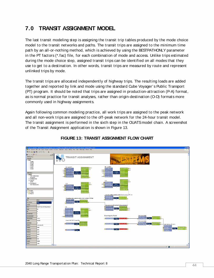
2040 Long Range Transportation Plan: Technical Report 8 44
7.0 TRANSIT ASSIGNMENT MODEL The last transit modeling step is assigning the transit trip tables produced by the mode choice model to the transit networks and paths. The transit trips are assigned to the minimum time path by an all-or-nothing method, which is achieved by using the BESTPATHONLY parameter in the PT factors (*.fac) file, for each combination of mode and access. Unlike trips estimated during the mode choice step, assigned transit trips can be identified on all modes that they use to get to a destination. In other words, transit trips are measured by route and represent unlinked trips by mode. The transit trips are allocated independently of highway trips. The resulting loads are added together and reported by link and mode using the standard Cube Voyager’s Public Transport (PT) program. It should be noted that trips are assigned in production-attraction (P-A) format, as is normal practice for transit analyses, rather than origin-destination (O-D) formats more commonly used in highway assignments. Again following common modeling practice, all work trips are assigned to the peak network and all non-work trips are assigned to the off-peak network for the 24-hour transit model. The transit assignment is performed in the sixth step in the OUATS model chain. A screenshot of the Transit Assignment application is shown in Figure 13.
FIGURE 13: TRANSIT ASSIGNMENT FLOW CHART

2040 Long Range Transportation Plan: Technical Report 8 45
This application assigns the transit vehicle trips to the highway and transit networks for 2009. In this version of the model, transit assignment is performed before highway assignment. The reason for doing this is that the auto access trips, from the home to park-n-ride locations, are recorded in a separate matrix. These trips are then later assigned along with other highway trips during the highway assignment. The Cube Voyager’s Public Transport (PT) program is used to perform transit assignment. The procedures are in place to accommodate future modeling applications for fixed guide way, and rail modes.
7.1 Transit Network Development The transit network was coded using the LYNX bus route schedules effective December, 2009. This included coding in the proper headways, bus stop locations, and other various transit route characteristics for each route. Both local bus routes and express bus routes were coded into the network as well as LYMMO, the Downtown Orlando circulator route.
7.2 Transit Assignment Methodology and Operation The transit assignment process loads a transit passenger trip table onto a transit network. The loading is performed on the minimum paths, which were created for each transit assignment mode -- local bus with walk access, line haul with local bus and walk access, and line haul with auto access -- in the transit application of the OUATS model. Two main options are used in this assignment process. The first of these is the transit line loading, which generates a sorted LEGS file for the future reporting of the transit line loads. The second is the non-transit link loading, which is reported as a feature of this process. In addition to the above procedures, a mode-to-mode transfer report is generated to show how the walk, auto, and transit modes interact and transfer people from one mode to another. This feature is repeated for each of the transit mode functions (local bus with walk access, line haul with local bus and walk access, and line haul with auto access). In the OUATS model, various input files containing transit operational characteristics are used in building the transit network, skimming the transit paths, and subsequently in the transit assignment process. There are many visualization improvements with the Cube Voyager OUATS transit assignment. One key feature of the transit assignment is the ability to observe the boardings and alightings at every stop of a transit route. Figure 14 shows a screenshot of a downtown route, LYNX’s LYMMO system, with the vertical bars representing boardings and de-boardings at every stop of the route.
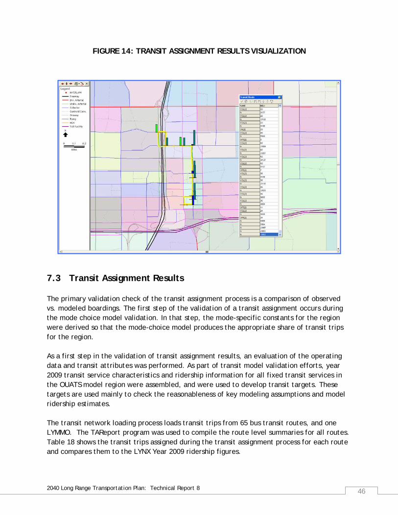
2040 Long Range Transportation Plan: Technical Report 8 46
FIGURE 14: TRANSIT ASSIGNMENT RESULTS VISUALIZATION
7.3 Transit Assignment Results The primary validation check of the transit assignment process is a comparison of observed vs. modeled boardings. The first step of the validation of a transit assignment occurs during the mode choice model validation. In that step, the mode-specific constants for the region were derived so that the mode-choice model produces the appropriate share of transit trips for the region. As a first step in the validation of transit assignment results, an evaluation of the operating data and transit attributes was performed. As part of transit model validation efforts, year 2009 transit service characteristics and ridership information for all fixed transit services in the OUATS model region were assembled, and were used to develop transit targets. These targets are used mainly to check the reasonableness of key modeling assumptions and model ridership estimates. The transit network loading process loads transit trips from 65 bus transit routes, and one LYMMO. The TAReport program was used to compile the route level summaries for all routes. Table 18 shows the transit trips assigned during the transit assignment process for each route and compares them to the LYNX Year 2009 ridership figures.
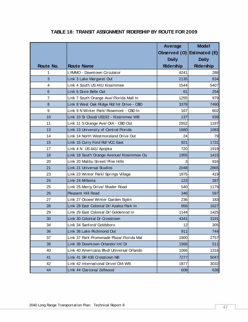
2040 Long Range Transportation Plan: Technical Report 8 47
TABLE 18: TRANSIT ASSIGNMENT RIDERSHIP BY ROUTE FOR 2009
Route No. Route Name
Average Observed (O)
Daily Ridership
Model Estimated (E)
Daily Ridership
1 LYMMO - Downtown Circulator 4241 288
3 Link 3 Lake Margaret Out 2135 834
4 Link 4 South US 441/Kissimmee 1544 5407
6 Link 6 Dixie Belle Out 61 254
7 Link 7 South Orange Ave/Florida Mall In 1255 979
8 Link 8 West Oak Ridge Rd/Int Drive - CBD 3378 7490
9 Link 9 N Winter Park/Rosemont - CBD In 167 602
10 Link 10 St Cloud/US192 - Kissimmee WB 137 939
11 Link 11 S Orange Ave/OIA - CBD Out 2552 1197
13 Link 13 University of Central Florida 1680 1083
14 Link 14 North Westmoreland Drive Out 24 79
15 Link 15 Curry Ford Rd/VCC East 921 1731
17 Link 4 N. US 441/Apopka 720 1919
18 Link 18 South Orange Avenue/Kissimmee Ou 1955 1415
20 Link 20 Malibu Street/Pine Hills 3 916
21 Link 21 Universal Studios 2048 2865
23 Link 23 Winter Park/Springs Village 1975 419
24 Link 24 Millenia 123 287
25 Link 25 Mercy Drive/Shader Road 540 1179
26 Pleasent Hill Road 346 597
27 Link 27 Ocoee/Winter Garden Siplin 236 183
28 Link 28 East Colonial Dr/Azalea Park In 956 1627
29 Link 29 East Colonial Dr/Goldenrod In 1144 1425
30 Link 30 Colonial Dr Crosstown 4341 3191
34 Link 34 Sanford/Goldsboro 12 305
36 Link 36 Lake Richmond Out 911 744
37 Link 37 Park Promenade Plaza/Florida Mal 1900 2757
38 Link 38 Downtown Orlando/Intl Dr 1566 511
40 Link 40 Americana Blvd/Universal Orlando 1066 1316
41 Link 41 SR 436 Crosstown NB 7277 5047
42 Link 42 International Drive/OIA WB 1877 3032
44 Link 44 Clarcona/Zellwood 608 636

2040 Long Range Transportation Plan: Technical Report 8 48
TABLE 18: TRANSIT ASSIGNMENT RIDERSHIP BY ROUTE FOR 2009 (CONT’D)
Route No. Route Name
Average Observed (O)
Daily Ridership
Model Estimated (E)
Daily Ridership
45 Link 45 Lake Mary 103 178
46 Link 46 West SR 46/Seminole Towne Center 145 541
48 Link 48 W Colonial Dr/Pk Promenade Plaza 1459 1947
49 Link 49 West Colonial Dr/Pine Hills Rd I 1557 1699
50 Link 50 Downtown Orlando/Magic Kingdom S 496 1985
51 Link 51 Conway/OIA Out 2782 872
54 Link 54 Old Winter Garden Rd In 305 491
55 Link 55 West U.S. 192/Four Corners Out 298 0
56 Link 56 West US 192/Magic Kingdom WB 595 0
57 Link 57 John Young Parkway 826 0
58 Link 58 Shingle Creek Circulator 60 0
102 Link 102 Orange Ave/South 17-92 7526 2413
103 Link 103 North 17-92 Sanford 1905 1145
111 Link 111 OIA/Disney 667 431
125 Link 125 Silver Star Rd Crosstown 3679 2156
200 Xpress Link 200 I-4 Express 6 52
301 Link 301 - Pine Hills/Animal Kingdom 59 159
302 Link 302 - Rosemont/Magic Kingdom 16 125
303 Link 303 - Washington Shores/MGM 96 98
304 Link 304 - Rio Grands/Vistana Res 4 148
305 Link 305 MetroWest 42 57
306 Link 306 Poinciana/Downtown Disney Tran 7 0
313 Link 313 VA Clinic 299 283
319 Link 19 Richmond Heights Out 909 1374
405 Link 405 Apopka-Park Ave 7 306
426 Link 426 Pleasent Hill Road/Poinciana 487 51
434 Link 434 SR 434 Crosstown 283 127
442 Link 442 Winter Garden Village 62 250
443 Link 443 Lee Road Crosstown 418 934
TOTAL 72797 69076

2040 Long Range Transportation Plan: Technical Report 8 49
A script was added to the transit assignment model to automatically generate the comparison of counted and modeled riders by the route.ent process for each route and compares them to the LYNX Year 2009 ridership figures.
8.0 APPLICATION GUIDELINES This section is intended to provide users of the MetroPlan Orlando travel demand model for the 2040 LRTP, guidance in the installation and usage of the OUATS CUBE/Voyager based model. It is advised that potential users go through training courses provided by FDOT in the use of the Florida Standard Urban Transportation Structure (FSUTMS) and the CUBE/Voyager software. Information regarding the courses can be obtained from www.FSUTMSOnline.net.
8.1 Minimum System Requirements In order to run the OUATS 2040 travel demand model, the following minimum specifications for software and hardware should be met: Cube Base version 5.1.2, Cube Voyager, FSUTMS v5.5, 2.0 GHz processor, 512 MB RAM, and 10 GB of disk space
Attempting to run the OUATS 2040 model without adhering to these minimum specifications will possibly lead to the model crashing and/or very long run times.
8.2 Directory Structure The OUATS 2040 LRTP Model directory is set up consistent with many of the existing regional models across the State of Florida. The main model folder, by default, is located under C:\FSUTMS in the District 5 (d5) folder. The folder structure should look like this c:\FSUTMS\d5\OUATS.40. After receiving the model DVD from MetroPlan Orlando, the first step is to copy all the model files, ensuring the computer meets the above minimum specifications. The OUATS.40 folder should be copied to the computer’s “C” drive. If an FSUTMS\d5 folder does not already exist on the “C” drive, it should be created. The OUATS.40 folder will then need to be copied into C:\FSUTMS\d5 from the DVD. Once the folder has been copied, right-click on the folder and go to “properties.” In the General tab, uncheck the “read-only” button and apply, respond

2040 Long Range Transportation Plan: Technical Report 8 50
with “OK” to change all files in the folder and subfolders. To open the model, click on the OUATS.cat file. If the model files are in the C:\FSUTMS\d5\OUATS.40 folder, the model is ready to be used. If the model is intended to run off a drive other than “C”, then the drive references must be changed (the user must respond to CUBE/Voyager prompts requesting the acceptance of the alternate folder location). In the OUATS.40 folder, there are five (5) subdirectories (Applications, Base, GIS, Parameters, and User.prg), a model catalog file (OUATS.cat), and an image file of the FSUTMS title bar (TITLEBAR.bmp) as shown in Figure 15.
FIGURE 15: FILE FOLDER TREE
8.2.1 Base Folder The base folder contains all of the various scenarios, model networks, and model data. The standard OUATS model comes with the following folders, each representing a different scenario: Base (2009 base year), EC2040 (2015 Existing-plus-committed network with 2040 SE data), CF2020 (year 2020 Cost Feasible Plan), CF2025 (year 2025 Cost Feasible Plan), CF2030 (year 2030 Cost Feasible Plan), CF2040 (year 2040 Cost Feasible Plan), and NE2040 (year 2040 Needs Plan)
The Base folder contains the Base 2009 model scenario with folders housing the input and output files. Also included as child scenarios are all of the future and interim model years, each with its own input and output folders.

2040 Long Range Transportation Plan: Technical Report 8 51
8.2.1.1 Input Folder The input folders are inside the Base folder, and each of the individual scenario folders. All files in the Input folder, with the exception of the PROFILE.mas file, include “yyb” in the name. The “yy” stands for the last two digits of the year and “b” represents a letter used to distinguish different scenarios. The model uses separate folders for each scenario, so it is important to follow this naming convention. If network changes are to be made or data interpolated to an interim year, a new folder can be created to differentiate between the networks. Make certain any network modifications are done in the “starting network” (box colored in red) for each scenario. 8.2.1.2 Output Folder The OUATS output folders are contained in the Base parent folder and under each child folder separately. Each scenario, upon completion, will contain all of the reports, trip tables, loaded networks, and other pertinent output data in this folder. The model will automatically carry over the naming convention. Figure 16 shows the main screen of the OUATS model. It includes a “Scenario” panel, an “Applications” panel, a ”Data” panel, and a “Keys” panel. When the “OUATS” application is invoked, the main flow chart appears. The OUATS 2040 Model is ready to be run.

2040 Long Range Transportation Plan: Technical Report 8 52
FIGURE 16: MAIN OUATS MODEL SCREEN
8.2.2 Parameters Folder The “Parameters” folder includes files used by all year models. These files are not year dependent and should remain unchanged to preserve the “calibration/validation” of the model. Files in the “Parameters” folder include the Speed/Capacity lookup table, trip attraction and production rates, friction factor curves, and mode choice constants and coefficients.
8.2.3 User.prg Folder The “User.prg” folder contains user-written programs that are not part of the Cube/Voyager suite of programs. The programs are mainly written in FORTRAN and are necessary to run the model. These include programs to run special attractions and the mode choice (and related utilities for auto and walk connectors).

2040 Long Range Transportation Plan: Technical Report 8 53
The files in the “User.prg” folder should not be changed in any way and should always remain under this folder for the model to run properly.
8.2.4 Applications Folder The “Applications” folder includes all Voyager scripting (*.s), application (*.app), and TMonitor (*.trf) files. These files are used to run the model. In addition, the folder has intermediate and temporary files created during a model run. Only experienced model users should modify any of the files in this folder.
8.2.5 GIS Folder The “GIS” folder contains geographic spatial reference files for the model such as Traffic Analysis Zone (TAZ) boundary, county boundary, hydrology, and street centerline files. The OUATS 2040 LRTP model uses the 1983 North American Datum (NAD) coordinate system (Florida East) in feet. The CUBE *.vpr files (user defined project files) provided with the OUATS model reference this GIS folder. The user can add files to this folder as needed.
8.3 Scenario Setup As mentioned earlier, there are various OUATS model scenarios included in the original Catalog file (OUATS.cat). Each one has been created to streamline and simplify the use of the model. A parent scenario is the basic one and usually differentiated by year. Under a parent there are child scenarios, which can be of the same year or different year as the parent but have different data such as different socio-economic data and/or network adjustments. A sibling is also a child of the parent scenario but different from another child. This nomenclature is commonly used to differentiate the positions relative to each other. Figure 16 shows the “Scenario” panel with the currently available scenario tree where Base is the parent, EC2040, CF2020, CF2025, CF2030, CF2040, and NE2040 are the “children” that are also “siblings” relative to each other.
8.3.1 Scenario Selection The OUATS 2040 model comes with eight (8) scenarios; a parent Base 2009, and children EC2040, NE2040, CF 2040, and four (4) interim children scenarios (CF2020, CF2025, and CF2030). As a scenario is selected, the input and output files in the flow chart change accordingly.
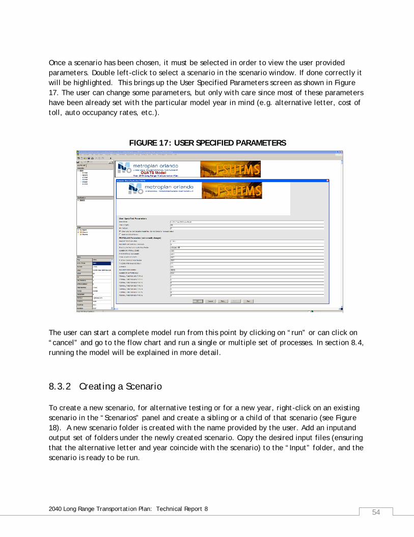
2040 Long Range Transportation Plan: Technical Report 8 54
Once a scenario has been chosen, it must be selected in order to view the user provided parameters. Double left-click to select a scenario in the scenario window. If done correctly it will be highlighted. This brings up the User Specified Parameters screen as shown in Figure 17. The user can change some parameters, but only with care since most of these parameters have been already set with the particular model year in mind (e.g. alternative letter, cost of toll, auto occupancy rates, etc.).
FIGURE 17: USER SPECIFIED PARAMETERS The user can start a complete model run from this point by clicking on “run” or can click on “cancel” and go to the flow chart and run a single or multiple set of processes. In section 8.4, running the model will be explained in more detail.
8.3.2 Creating a Scenario To create a new scenario, for alternative testing or for a new year, right-click on an existing scenario in the “Scenarios” panel and create a sibling or a child of that scenario (see Figure 18). A new scenario folder is created with the name provided by the user. Add an inputand output set of folders under the newly created scenario. Copy the desired input files (ensuring that the alternative letter and year coincide with the scenario) to the “Input” folder, and the scenario is ready to be run.

2040 Long Range Transportation Plan: Technical Report 8 55
FIGURE 18: SCENARIO TREE
2040 Long Range Transportation Plan: Technical Report 8 56
8.4 Running the Model Once a scenario has been updated as needed or a new one has been created, the model is ready to be run. Running the model is a simple process; just double click on the desired scenario and when the scenario management interface window opens select the Run button on the lower right corner. To run just a single step within any process, just select the scenario and then double-click on the desired step or press F2. When the “Run Application” window opens select “Run Application,” and only that step will run. After the model is finished running, all of the outputs will be in the output folder under the appropriate scenario. All files created (text, database, matrix, networks, etc. type files) can be opened using CUBE by double-clicking on the appropriate box in the flow chart. The 2009 base year model was run on a desktop PC with a single core Xeon machine at 3 GHz clock speed using Windows XP Professional and with 1 GB of memory (RAM). The output folder required 663 MB of hard disk space while the “Applications” folder ended up with an additional 671 MB of disk space. The model ran in just under four (4) hours. The same model on a dual quad core (eight processors at 2 GHz each) machine with Windows XP Professional (64-bit version) with 8 GB of memory (RAM) ran in two (2) hours and 48 minutes.

2040 Long Range Transportation Plan: Technical Report 8 57
APPENDIX A:
EXTERNAL TRIPS
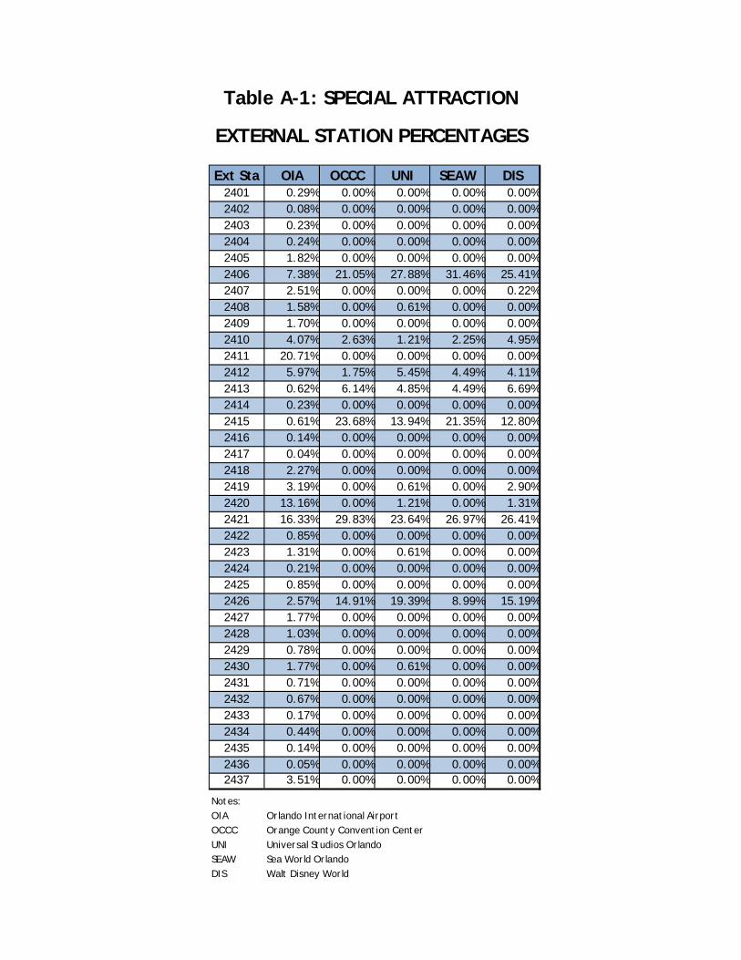
Table A-1: SPECIAL ATTRACTION
EXTERNAL STATION PERCENTAGES
Ext Sta OIA OCCC UNI SEAW DIS2401 0.29% 0.00% 0.00% 0.00% 0.00%2402 0.08% 0.00% 0.00% 0.00% 0.00%2403 0.23% 0.00% 0.00% 0.00% 0.00%2404 0.24% 0.00% 0.00% 0.00% 0.00%2405 1.82% 0.00% 0.00% 0.00% 0.00%2406 7.38% 21.05% 27.88% 31.46% 25.41%2407 2.51% 0.00% 0.00% 0.00% 0.22%2408 1.58% 0.00% 0.61% 0.00% 0.00%2409 1.70% 0.00% 0.00% 0.00% 0.00%2410 4.07% 2.63% 1.21% 2.25% 4.95%2411 20.71% 0.00% 0.00% 0.00% 0.00%2412 5.97% 1.75% 5.45% 4.49% 4.11%2413 0.62% 6.14% 4.85% 4.49% 6.69%2414 0.23% 0.00% 0.00% 0.00% 0.00%2415 0.61% 23.68% 13.94% 21.35% 12.80%2416 0.14% 0.00% 0.00% 0.00% 0.00%2417 0.04% 0.00% 0.00% 0.00% 0.00%2418 2.27% 0.00% 0.00% 0.00% 0.00%2419 3.19% 0.00% 0.61% 0.00% 2.90%2420 13.16% 0.00% 1.21% 0.00% 1.31%2421 16.33% 29.83% 23.64% 26.97% 26.41%2422 0.85% 0.00% 0.00% 0.00% 0.00%2423 1.31% 0.00% 0.61% 0.00% 0.00%2424 0.21% 0.00% 0.00% 0.00% 0.00%2425 0.85% 0.00% 0.00% 0.00% 0.00%2426 2.57% 14.91% 19.39% 8.99% 15.19%2427 1.77% 0.00% 0.00% 0.00% 0.00%2428 1.03% 0.00% 0.00% 0.00% 0.00%2429 0.78% 0.00% 0.00% 0.00% 0.00%2430 1.77% 0.00% 0.61% 0.00% 0.00%2431 0.71% 0.00% 0.00% 0.00% 0.00%2432 0.67% 0.00% 0.00% 0.00% 0.00%2433 0.17% 0.00% 0.00% 0.00% 0.00%2434 0.44% 0.00% 0.00% 0.00% 0.00%2435 0.14% 0.00% 0.00% 0.00% 0.00%2436 0.05% 0.00% 0.00% 0.00% 0.00%2437 3.51% 0.00% 0.00% 0.00% 0.00%
Notes:OIA Orlando International AirportOCCC Orange County Convention CenterUNI Universal Studios OrlandoSEAW Sea World OrlandoDIS Walt Disney World

Table A-2: EXTERNAL TRIP BREAKDOWN
Ext Sta Count Auto EI Auto EE LT EI LT EE HT EI HT EE OIA EI OCCC EI UNI EI SEAW DIS EI2401 5,100 3,527 675 199 3 272 3 35 0 0 0 02402 1,150 1,040 57 30 0 30 0 9 0 0 0 02403 2,390 2,016 236 166 2 166 2 27 0 0 0 02404 5,700 1,863 60 22 2 419 27 28 0 0 0 02405 14,250 11,724 2 1,513 0 0 0 218 0 0 0 02406 58,334 33,469 4,565 6,642 165 3,322 83 881 4,356 3,388 2,098 2,7562407 15,100 12,702 178 0 0 1,600 2 299 0 0 0 242408 9,000 7,911 23 530 0 466 0 188 0 74 0 02409 5,900 4,775 25 380 0 380 0 203 0 0 0 02410 12,500 10,229 881 404 2 404 2 486 544 147 150 5372411 39,814 32,041 1,221 0 0 3,075 17 2,472 0 0 0 02412 14,400 11,966 77 480 0 940 0 713 362 662 299 4462413 6,200 2,408 559 1,046 33 148 5 74 1,271 589 299 7262414 5,818 1,634 205 377 153 832 338 28 0 0 0 02415 27,010 5,411 3,260 958 1,750 1,202 2,195 73 4,901 1,694 1,424 1,3882416 3,020 1,795 66 31 0 63 0 17 0 0 0 02417 6,900 414 0 75 1,484 182 3,556 4 0 0 0 02418 6,000 5,254 0 567 0 52 0 272 0 0 0 02419 11,086 8,992 0 1,337 0 532 0 381 0 74 0 3152420 52,198 36,071 5,246 3,248 226 3,712 258 1,571 0 147 0 1432421 72,872 34,420 6,497 7,189 868 9,743 1,177 1,949 6,171 2,873 1,798 2,8642422 5,686 3,228 599 324 0 1,275 1 101 0 0 0 02423 7,700 4,764 368 2,149 0 0 0 156 0 74 0 02424 2,226 1,588 550 44 0 44 0 25 0 0 0 02425 5,310 3,858 0 91 0 1,277 0 101 0 0 0 02426 37,978 9,446 1,425 3,894 4,470 2,755 3,163 307 3,086 2,356 599 1,6472427 14,600 11,390 221 930 0 1,516 0 211 0 0 0 02428 8,872 8,317 110 222 0 222 0 122 0 0 0 02429 7,450 6,966 110 187 0 187 0 93 0 0 0 02430 18,700 15,894 534 936 0 346 0 211 0 74 0 02431 7,070 5,776 0 350 0 789 0 85 0 0 0 02432 5,382 5,108 0 137 0 137 0 80 0 0 0 02433 1,396 1,324 0 36 0 36 0 21 0 0 0 02434 3,522 2,777 32 127 0 381 0 52 0 0 0 02435 2,024 1,545 0 234 0 234 0 17 0 0 0 02436 4,600 436 1,023 40 507 165 2,028 5 0 0 0 02437 9,600 9,120 0 384 0 96 0 419 0 0 0 0
2040 Long Range Transportation Plan: Technical Report 8 60
APPENDIX B:
SOCIO-ECONOMIC DATA
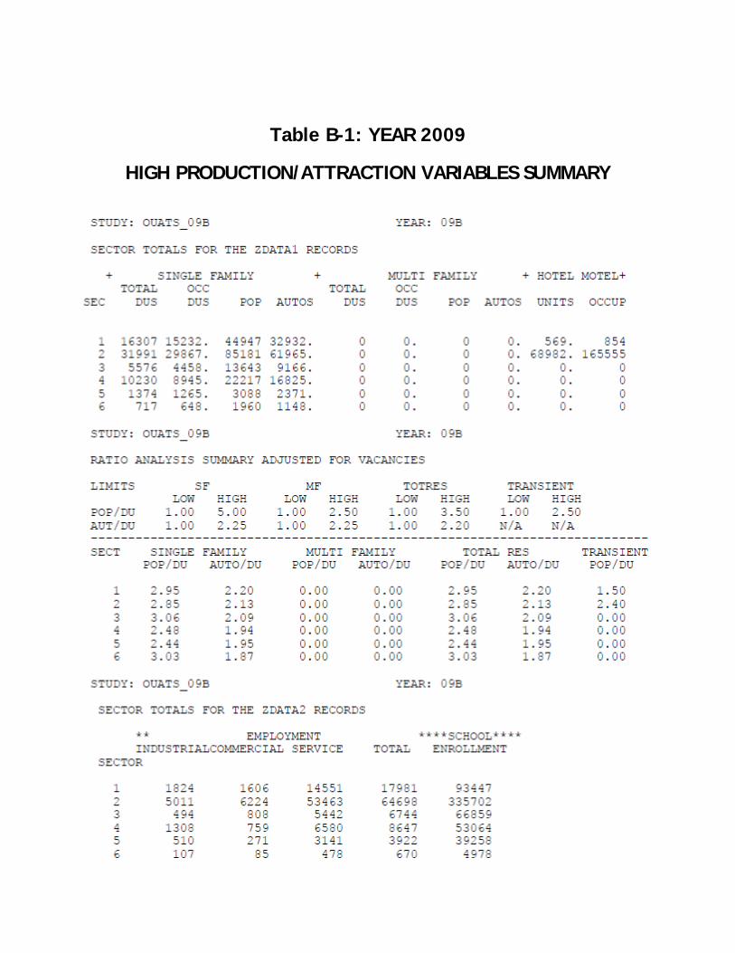
Table B-1: YEAR 2009
HIGH PRODUCTION/ATTRACTION VARIABLES SUMMARY

Table B-2: YEAR 2009
MEDIUM PRODUCTION/ATTRACTION VARIABLES SUMMARY
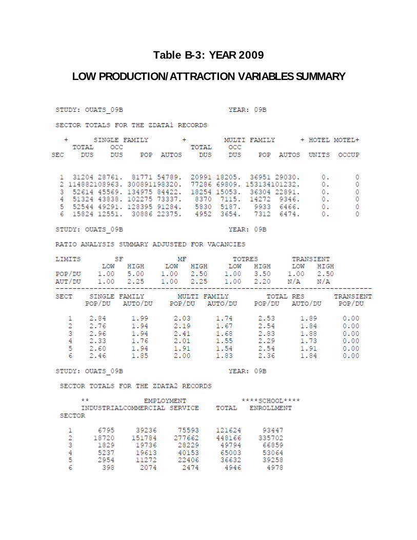
Table B-3: YEAR 2009
LOW PRODUCTION/ATTRACTION VARIABLES SUMMARY

FIGURE B-1: SEMINOLE COUNTY TAZ MAP
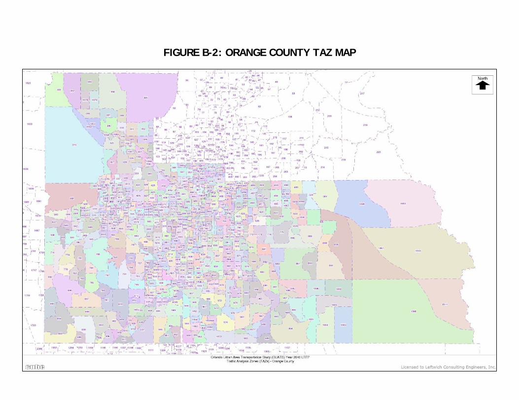
FIGURE B-2: ORANGE COUNTY TAZ MAP

FIGURE B-3: OSCEOLA COUNTY TAZ MAP

FIGURE B-4: LAKE COUNTY TAZ MAP

FIGURE B-5: WEST VOLUSIA COUNTY TAZ MAP

FIGURE B-6: NORTH EAST POLK COUNTY TAZ MAP

TABLE B-4
ZONEDATA_YYA.DBF FILE VARIABLE DESCRIPTION
Variable Name Type Width Description Z Number 9 TAZ Number CTY Number 9 County Location DUS_ALL Number 9 Total Single-Family Dwelling Units (SF DUs) PCVTS_ALL Number 9 Total % Seasonal + Vacant SF DUs PCVS ALL Number 9 Total % Vacant SF DUs POPS_ALL Number 9 Total Population in SF DUs PCAl l ALL Number 9 Total % 0 Vehicles in SF DUs PCAl2 ALL Number 9 Total % 1 Vehicle in SF DUs PCA13_ALL Number 9 Total % 2+ Vehicles in SF DUs DUM ALL Number 9 Total Multi-Family Dwelling Units (MF DUs) PCVTM_ALL Number 9 Total % Seasonal + Vacant MF DUs PCVM ALL Number 9 Total % Vacant MF DUs POPM_ALL Number 9 Total Population in MF DUs PCA21_ALL Number 9 Total % 0 Vehicles in MF DUs PCA22 ALL Number 9 Total % 1 Vehicle in MF DUs PCA23_ALL Number 9 Total % 2+ Vehicles in MF DUs DUH_ALL Number 9 Total Number of Hotel Rooms PCOH_ALL Number 9 Total % Occupied POPH_ALL Number 9 Total Population in Hotel Rooms DUS Number 9 High Income Single-Family Dwelling Units PCVTS Number 9 High Income % Seasonal + Vacant SF DUs PCVS_HI Number 9 High income % Vacant SF DUs POPS_HI Number 9 High Income Population in SF DUs PCA11_H I Number 9 High Income % 0 Vehicles in SF DUs PCAl2 _HI Number 9 High Income % 1 Vehicle in SF DUs PCA13_FII Number 9 High Income % 2+ Vehicles in SF DUs DUM_HI Number 9 High Income Multi-Family Dwelling Units PCVTM_HI Number 9 High Income % Seasonal + Vacant MF DUs PCVM_HI Number 9 High Income % Vacant MF DUs POPM Number 9 High Income Population in MF DUs PCA21J-II Number 9 High Income % 0 Vehicles in MF DUs PCA22_HI Number 9 High Income % 1 Vehicle in MF DUs PCA23_HI Number 9 High Income % 2+ Vehicles in MF DUs DUH_HI Number 9 High Income Number of Hotel Rooms PCOH _HI Number 9 High Income % Occupied POPH_HI Number 9 High Income Population in Hotel Rooms DUS_ME Number 9 Medium Income Single-Family Dwelling Units PCVTS_ME Number 9 Medium Income % Seasonal + Vacant SF DUs PCVM_ME Number 9 Medium Income % Vacant SF DUs POPS_ ME Number 9 Medium Income Population in SF DUs PCA11_ME Number 9 Medium Income % 0 Vehicles in SF DUs PCAl2_ME Number 9 Medium Income % 1 Vehicle in SF DUs PCA13_ME Number 9 Medium Income % 2+ Vehicles in SF DUs DUM_ME Number 9 Medium Income Multi-Family Dwelling Units PCVTM_ME Number 9 Medium Income % Seasonal + Vacant MF DUs PCVM_ME Number 9 Medium Income % Vacant MF DUs POPM_ME Number 9 Medium Income Population in MF DUs PCA21_ME Number 9 Medium Income % 0 Vehicles in MF DUs PCA22_ME Number 9 Medium Income % 1 Vehicle in MF DUs PCA23_ME Number 9 Medium Income % 2+ Vehicles in MF DUs DUH_ME Number 9 Medium Income Number of Hotel Rooms

TABLE B-4:(CONT’D)
ZONEDATA_YYA.DBF FILE VARIABLE DESCRIPTION
Variable Name Type Width Description PCOH_ME Number 9 Medium Income % Occupied POPH_M E Number 9 Medium Income Population in Hotel Rooms DUS_LO Number 9 Low Income Single-Family Dwelling Units PCVTS_LO Number 9 Low Income % Seasonal + Vacant SF DUs PCVS_LO Number 9 Low Income % Vacant SF DUs POPM_LO Number 9 Low Income Population in SF DUs PCA11_LO Number 9 Low Income % 0 Vehicles in SF DUs PCAl2_LO Number 9 Low Income % 1 Vehicle in SF DUs PCA13_LO Number 9 Low Income % 2+ Vehicles in SF DUs DUM_LO Number 9 Low Income Multi-Family Dwelling Units PCVTM_LO Number 9 Low Income % Seasonal + Vacant MF DUs PCVM_LO Number 9 Low Income % Vacant MF DUs POPM_LO Number 9 Low Income Population in MF DUs PCA21_LO Number 9 Low Income % 0 Vehicles in MF DUs PCA223.0 Number 9 Low Income % 1 Vehicle in ME DUs PCA23 LO Number 9 Low Income % 2+ Vehicles in ME DUs DUHLO Number 9 Low Income Number of Hotel Rooms PCOH_LO Number 9 Low Income % Occupied POPH_LO Number 9 Low Income Population in Hotel Rooms IND_ALL Number 9 Total Industrial Employment COM ALL Number 9 Total Commercial Employment SVC ALL Number 9 Total Service Employment TOEMP_ALL Number 9 Total Employment SCHENR Number 9 Total School Enrollment IND_HI Number 9 High Income Industrial Employment COM HI Number 9 High Income Commercial Employment SVC _HI Number 9 High Income Service Employment TOEMP_HI Number 9 High Income Total Employment IND ME Number 9 Medium Income Industrial Employment COM_ME Number 9 Medium Income Commercial Employment SVC _ME Number 9 Medium Income Service Employment TOEMP_ME Number 9 Medium Income Total Employment I ND_LO Number 9 Low Income Industrial Employment COM_LO Number 9 Low Income Commercial Employment SVC_LO Number 9 Low Income Service Employment TOEMPLO Number 9 Low Income Total Employment

Table B-5: TRAFFIC ANALYSIS ZONE RANGES BY COUNTY
2030 LRTP 2040 LRTPCounty Model TAZ No. Model TAZ No.Seminole 1-300 1-300Orange 301-1100 301-1100Osceola 1101-1300 1101-1400Lake 1301-1600 1401-1800Volusia 1601-1900 1801-2300Polk 1901-2000 2301-2400External Stations 2001-2037 2401-2437

2040 Long Range Transportation Plan: Technical Report 8 73
APPENDIX C:
TRIP GENERATION
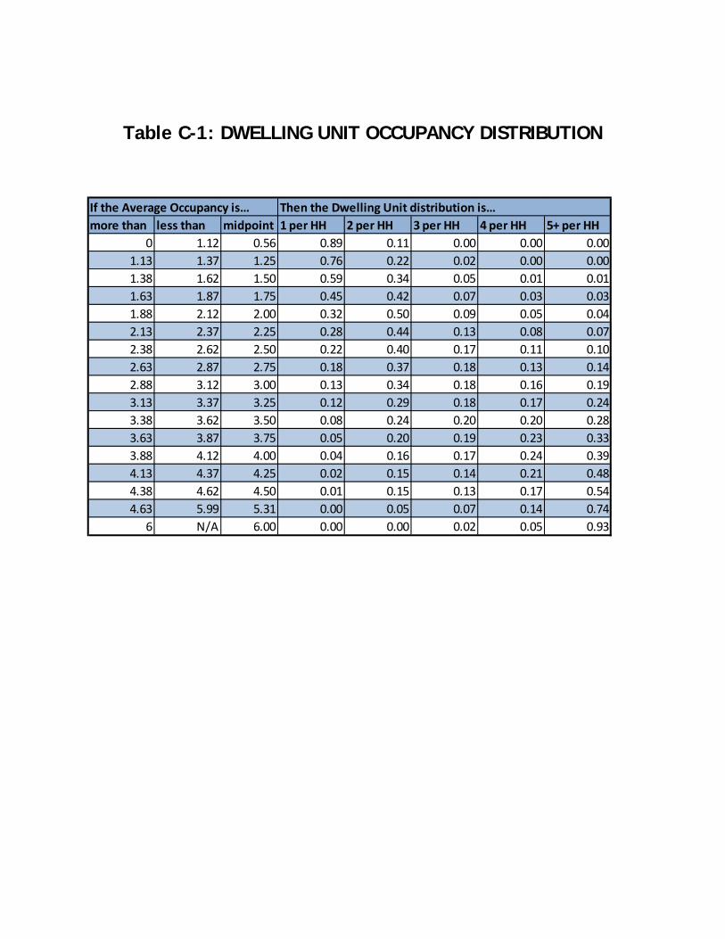
Table C-1: DWELLING UNIT OCCUPANCY DISTRIBUTION
more than less than midpoint 1 per HH 2 per HH 3 per HH 4 per HH 5+ per HH0 1.12 0.56 0.89 0.11 0.00 0.00 0.00
1.13 1.37 1.25 0.76 0.22 0.02 0.00 0.001.38 1.62 1.50 0.59 0.34 0.05 0.01 0.011.63 1.87 1.75 0.45 0.42 0.07 0.03 0.031.88 2.12 2.00 0.32 0.50 0.09 0.05 0.042.13 2.37 2.25 0.28 0.44 0.13 0.08 0.072.38 2.62 2.50 0.22 0.40 0.17 0.11 0.102.63 2.87 2.75 0.18 0.37 0.18 0.13 0.142.88 3.12 3.00 0.13 0.34 0.18 0.16 0.193.13 3.37 3.25 0.12 0.29 0.18 0.17 0.243.38 3.62 3.50 0.08 0.24 0.20 0.20 0.283.63 3.87 3.75 0.05 0.20 0.19 0.23 0.333.88 4.12 4.00 0.04 0.16 0.17 0.24 0.394.13 4.37 4.25 0.02 0.15 0.14 0.21 0.484.38 4.62 4.50 0.01 0.15 0.13 0.17 0.544.63 5.99 5.31 0.00 0.05 0.07 0.14 0.74
6 N/A 6.00 0.00 0.00 0.02 0.05 0.93
If the Average Occupancy is… Then the Dwelling Unit distribution is…

Table C-2: SEMINOLE COUNTY TRIP GENERATION RATES
UnitType HBW HBSH HBSR HBO
SF 0.147 0.203 0.102 0.203MF 0.203 0.203 0.147 0.203Hotel 0.124 0.147 0.304 0.253SF 0.349 0.304 0.304 0.405MF 0.455 0.253 0.253 0.405Hotel 0.124 0.147 0.304 0.253SF 0.754 0.585 0.304 0.630MF 0.658 0.405 0.304 0.608Hotel 0.124 0.147 0.304 0.253SF 0.253 0.230 0.124 0.253MF 0.304 0.230 0.169 0.349Hotel 0.102 0.653 0.838 0.608SF 0.557 0.557 0.349 0.912MF 0.557 0.585 0.327 0.653Hotel 0.102 0.653 0.838 0.608SF 0.962 0.687 0.383 1.013MF 0.912 0.709 0.349 0.934Hotel 0.102 0.653 0.838 0.608SF 0.455 0.253 0.147 0.507MF 0.405 0.253 0.203 0.507Hotel 0.079 1.013 1.362 1.063SF 0.754 0.653 0.455 1.648MF 0.754 0.754 0.383 1.317Hotel 0.079 1.013 1.362 1.063SF 1.165 0.754 0.507 1.862MF 1.063 0.934 0.405 1.772Hotel 0.079 1.013 1.362 1.063SF 0.608 0.282 0.169 0.754MF 0.507 0.282 0.230 0.754Hotel 0.045 1.260 1.969 1.670SF 0.815 0.732 0.557 2.323MF 0.815 0.912 0.455 1.817Hotel 0.045 1.260 1.969 1.670SF 1.265 1.013 0.630 2.835MF 1.114 1.063 0.529 2.683Hotel 0.045 1.260 1.969 1.670SF 0.658 0.304 0.203 1.108MF 0.557 0.304 0.253 1.013Hotel 0.045 1.468 2.987 2.222SF 0.860 0.754 0.709 3.240MF 0.860 0.957 0.608 2.278Hotel 0.045 1.468 2.987 2.222SF 1.317 1.260 0.777 3.640MF 1.165 1.137 0.810 3.290Hotel 0.045 1.468 2.987 2.222
Purpose Ind Emp Com Emp Svc Emp Tot Emp Tot Dus T/THBW 0.00 0.00 0.00 1.74 0.00 0.00HBSH 0.00 5.90 0.00 0.00 0.00 0.00HBSR 0.00 1.45 1.45 0.00 0.48 0.00HBO 0.00 1.26 1.26 0.00 0.20 1.26NHB 0.00 2.81 1.36 0.00 0.30 0.00T/T 0.00 0.00 0.00 0.41 0.30 0.00
Attraction Rates
2
3
4
5
Autos Per DU
Production Rates
1
2
3
1
2
3
1
2
3
1
2
3
Persons Per DU
Trip Purposes
1
2
3
1

Table C-3: ORANGE COUNTY TRIP GENERATION RATES
UnitType HBW HBSH HBSR HBO
SF 0.163 0.222 0.105 0.222MF 0.222 0.222 0.163 0.222Hotel 0.128 0.163 0.321 0.268SF 0.373 0.321 0.321 0.432MF 0.484 0.268 0.268 0.432Hotel 0.128 0.163 0.321 0.268SF 0.811 0.618 0.321 0.671MF 0.706 0.432 0.321 0.642Hotel 0.128 0.163 0.321 0.268SF 0.268 0.245 0.128 0.268MF 0.321 0.245 0.193 0.373Hotel 0.105 0.706 0.887 0.642SF 0.595 0.595 0.373 0.968MF 0.595 0.618 0.350 0.706Hotel 0.105 0.706 0.887 0.642SF 1.015 0.723 0.403 1.079MF 0.968 0.758 0.373 0.992Hotel 0.105 0.706 0.887 0.642SF 0.484 0.268 0.163 0.537MF 0.432 0.268 0.222 0.537Hotel 0.082 1.079 1.453 1.132SF 0.811 0.706 0.484 1.744MF 0.811 0.811 0.403 1.400Hotel 0.082 1.079 1.453 1.132SF 1.237 0.811 0.537 1.989MF 1.132 0.992 0.432 1.890Hotel 0.082 1.079 1.453 1.132SF 0.642 0.292 0.193 0.811MF 0.537 0.292 0.245 0.811Hotel 0.053 1.348 2.094 1.779SF 0.863 0.782 0.595 2.468MF 0.863 0.968 0.484 1.937Hotel 0.053 1.330 2.094 1.779SF 1.348 1.079 0.671 3.016MF 1.184 1.132 0.566 2.858Hotel 0.053 1.348 2.094 1.779SF 0.706 0.321 0.222 1.184MF 0.595 0.321 0.268 1.079Hotel 0.053 1.558 3.179 2.368SF 0.922 0.811 0.758 3.453MF 0.922 1.015 0.642 2.427Hotel 0.053 1.558 3.179 2.368SF 1.406 1.348 0.834 3.885MF 1.237 1.208 0.858 3.506Hotel 0.053 1.558 3.179 2.368
Purpose Ind Emp Com Emp Svc Emp Tot Emp Tot Dus T/THBW 0.00 0.00 0.00 1.74 0.00 0.00HBSH 0.00 5.89 0.00 0.00 0.00 0.00HBSR 0.00 1.46 1.46 0.00 0.49 0.00HBO 0.00 1.26 1.26 0.00 0.20 1.26NHB 0.00 2.81 1.70 0.00 0.29 0.00T/T 0.00 0.00 0.00 0.43 0.29 0.00
Attraction Rates
1
2
3
5
1
2
3
1
2
3
3
1
2
3
1
1
2
3
Autos Per DU
Trip PurposesPersons Per DU
2
4
Production Rates

Table C-4: OSCEOLA COUNTY TRIP GENERATION RATES
UnitType HBW HBSH HBSR HBO
SF 0.265 0.338 0.180 0.338MF 0.338 0.338 0.265 0.338Hotel 0.212 0.265 0.518 0.445SF 0.625 0.518 0.518 0.709MF 0.784 0.445 0.445 0.709Hotel 0.212 0.265 0.518 0.445SF 1.313 1.006 0.518 1.091MF 1.144 0.709 0.518 1.038Hotel 0.212 0.265 0.518 0.445SF 0.445 0.392 0.212 0.445MF 0.518 0.392 0.307 0.614Hotel 0.180 1.144 1.451 1.038SF 0.964 0.964 0.614 1.589MF 0.964 1.006 0.572 1.144Hotel 0.180 1.144 1.451 1.038SF 1.662 1.186 0.656 1.736MF 1.589 1.229 0.614 1.609Hotel 0.180 1.144 1.451 1.038SF 0.784 0.445 0.265 0.878MF 0.709 0.445 0.338 0.878Hotel 0.138 1.736 2.362 1.842SF 1.313 1.144 0.784 2.849MF 1.313 1.313 0.656 2.266Hotel 0.138 1.736 2.362 1.842SF 2.012 1.313 0.932 3.229MF 1.853 1.609 0.709 3.060Hotel 0.138 1.736 2.362 1.842SF 1.058 0.487 0.307 1.313MF 0.878 0.487 0.392 1.313Hotel 0.074 2.182 3.420 2.902SF 1.398 1.260 0.964 4.024MF 1.398 1.589 0.784 3.155Hotel 0.074 2.182 3.420 2.902SF 2.182 1.736 1.091 4.892MF 1.927 1.842 0.932 4.638Hotel 0.074 2.182 3.420 2.902SF 1.144 0.518 0.338 1.916MF 0.964 0.518 0.445 1.736Hotel 0.074 2.531 5.156 3.854SF 1.482 1.313 1.229 5.602MF 1.482 1.662 1.038 3.938Hotel 0.074 2.531 5.156 3.854SF 2.276 2.182 1.355 6.289MF 2.012 1.969 1.398 5.675Hotel 0.074 2.531 5.156 3.854
Purpose Ind Emp Com Emp Svc Emp Tot Emp Tot Dus T/THBW 0.00 0.00 0.00 2.62 0.00 0.00HBSH 0.00 8.84 0.00 0.00 0.00 0.00HBSR 0.00 2.17 2.17 0.00 0.73 0.00HBO 0.00 1.88 1.88 0.00 0.29 1.88NHB 0.00 4.20 2.03 0.00 0.44 0.00T/T 0.00 0.00 0.00 0.65 0.44 0.00
Production Rates
Attraction Rates
5
1
2
3
3
1
2
3
4
1
2
3
1
2
3
2
1
2
3
1
Persons Per DU
Autos Per DU
Trip Purposes

Table C-5: LAKE COUNTY TRIP GENERATION RATES
UnitType HBW HBSH HBSR HBO
SF 0.153 0.198 0.099 0.198MF 0.198 0.198 0.153 0.198Hotel 0.126 0.153 0.297 0.252SF 0.342 0.297 0.297 0.387MF 0.432 0.252 0.252 0.387Hotel 0.126 0.153 0.297 0.252SF 0.720 0.558 0.297 0.612MF 0.630 0.387 0.297 0.594Hotel 0.126 0.153 0.297 0.252SF 0.252 0.216 0.126 0.252MF 0.297 0.216 0.171 0.342Hotel 0.099 0.639 0.810 0.594SF 0.522 0.531 0.342 0.882MF 0.522 0.558 0.315 0.639Hotel 0.099 0.639 0.810 0.594SF 0.918 0.666 0.369 0.981MF 0.873 0.684 0.342 0.909Hotel 0.099 0.639 0.810 0.594SF 0.432 0.252 0.153 0.486MF 0.387 0.252 0.198 0.486Hotel 0.072 0.981 1.314 1.026SF 0.720 0.639 0.450 1.602MF 0.720 0.738 0.369 1.278Hotel 0.072 0.981 1.314 1.026SF 1.062 0.738 0.486 1.818MF 0.972 0.909 0.387 1.728Hotel 0.072 0.981 1.314 1.026SF 0.585 0.270 0.171 0.738MF 0.486 0.270 0.216 0.738Hotel 0.045 1.233 1.926 1.629SF 0.774 0.702 0.531 2.259MF 0.774 0.882 0.450 1.773Hotel 0.045 1.233 1.926 1.629SF 1.206 0.981 0.612 2.754MF 1.071 1.026 0.513 2.610Hotel 0.045 1.233 1.926 1.629SF 0.630 0.297 0.198 1.080MF 0.522 0.297 0.252 0.981Hotel 0.045 1.431 2.898 2.160SF 0.819 0.738 0.684 3.141MF 0.819 0.936 0.594 2.214Hotel 0.045 1.431 2.898 2.160SF 1.260 1.233 0.765 3.537MF 1.116 1.098 0.783 3.195Hotel 0.045 1.431 2.898 2.160
Purpose Ind Emp Com Emp Svc Emp Tot Emp Tot Dus T/THBW 0.00 0.00 0.00 1.74 0.00 0.00HBSH 0.00 5.90 0.00 0.00 0.00 0.00HBSR 0.00 1.46 1.46 0.00 0.49 0.00HBO 0.00 1.26 1.26 0.00 0.19 1.26NHB 0.00 2.81 1.35 0.00 0.30 0.00T/T 0.00 0.00 0.00 0.43 0.30 0.00
Production Rates
Attraction Rates
4
1
2
3
5
1
2
3
2
3
3
1
2
3
1
1
2
3
2
1
Autos Per DU
Trip PurposesPersons Per DU

Table C-6: VOLUSIA COUNTY TRIP GENERATION RATES
UnitType HBW HBSH HBSR HBO
SF 0.154 0.220 0.110 0.220MF 0.220 0.220 0.154 0.220Hotel 0.143 0.154 0.330 0.275SF 0.385 0.330 0.330 0.440MF 0.495 0.275 0.275 0.440Hotel 0.143 0.154 0.330 0.275SF 0.836 0.638 0.330 0.693MF 0.726 0.440 0.330 0.671Hotel 0.143 0.154 0.330 0.275SF 0.275 0.253 0.143 0.275MF 0.330 0.253 0.198 0.385Hotel 0.110 0.726 0.902 0.671SF 0.605 0.605 0.385 0.990MF 0.605 0.638 0.363 0.726Hotel 0.110 0.726 0.902 0.671SF 1.045 0.748 0.418 1.111MF 0.990 0.770 0.385 1.023Hotel 0.110 0.726 0.902 0.671SF 0.495 0.275 0.154 0.550MF 0.440 0.275 0.220 0.550Hotel 0.088 1.111 1.496 1.166SF 0.836 0.726 0.495 1.793MF 0.836 0.836 0.418 1.430Hotel 0.088 1.111 1.496 1.166SF 1.265 0.836 0.550 2.046MF 1.155 1.023 0.440 1.936Hotel 0.088 1.111 1.496 1.166SF 0.660 0.297 0.198 0.836MF 0.550 0.297 0.253 0.836Hotel 0.055 1.386 2.156 1.826SF 0.880 0.803 0.605 2.541MF 0.880 0.990 0.495 2.002Hotel 0.055 1.386 2.156 1.826SF 1.386 1.111 0.693 3.102MF 1.210 1.166 0.583 2.926Hotel 0.055 1.386 2.156 1.826SF 0.726 0.330 0.220 1.221MF 0.605 0.330 0.275 1.111Hotel 0.055 1.606 3.267 2.431SF 0.935 0.836 0.770 3.542MF 0.935 1.045 0.671 2.486Hotel 0.055 1.606 3.267 2.431SF 1.430 1.386 0.858 3.982MF 1.265 1.254 0.891 3.597Hotel 0.055 1.606 3.267 2.431
Purpose Ind Emp Com Emp Svc Emp Tot Emp Tot Dus T/THBW 0.00 0.00 0.00 1.74 0.00 0.00HBSH 0.00 5.90 0.00 0.00 0.00 0.00HBSR 0.00 1.46 1.46 0.00 0.49 0.00HBO 0.00 1.26 1.26 0.00 0.19 1.26NHB 0.00 2.81 1.36 0.00 0.29 0.00T/T 0.00 0.00 0.00 0.43 0.29 0.00
Production Rates
Attraction Rates
5
1
2
3
3
1
2
3
4
1
2
3
1
1
2
3
2
1
2
3
Persons Per DU
Autos Per DU
Trip Purposes

Table C-7: POLK COUNTY TRIP GENERATION RATES
UnitType HBW HBSH HBSR HBO
SF 0.077 0.110 0.055 0.110MF 0.110 0.110 0.077 0.110Hotel 0.066 0.077 0.154 0.132SF 0.187 0.154 0.154 0.209MF 0.242 0.132 0.132 0.209Hotel 0.066 0.077 0.154 0.132SF 0.396 0.308 0.154 0.330MF 0.341 0.209 0.154 0.319Hotel 0.066 0.077 0.154 0.132SF 0.132 0.121 0.066 0.132MF 0.154 0.121 0.088 0.187Hotel 0.055 0.341 0.440 0.319SF 0.286 0.286 0.187 0.473MF 0.286 0.308 0.176 0.341Hotel 0.055 0.341 0.440 0.319SF 0.506 0.363 0.198 0.528MF 0.473 0.374 0.187 0.495Hotel 0.055 0.341 0.440 0.319SF 0.242 0.132 0.077 0.264MF 0.209 0.132 0.110 0.264Hotel 0.044 0.528 0.715 0.550SF 0.396 0.341 0.242 0.858MF 0.396 0.396 0.198 0.682Hotel 0.044 0.528 0.715 0.550SF 0.605 0.396 0.264 0.990MF 0.550 0.495 0.209 0.935Hotel 0.044 0.528 0.715 0.550SF 0.319 0.154 0.088 0.396MF 0.264 0.154 0.121 0.396Hotel 0.022 0.660 1.034 0.869SF 0.418 0.385 0.286 1.221MF 0.418 0.473 0.242 0.946Hotel 0.022 0.660 1.034 0.869SF 0.660 0.528 0.330 1.485MF 0.583 0.550 0.286 1.408Hotel 0.022 0.660 1.034 0.869SF 0.341 0.154 0.110 0.583MF 0.286 0.154 0.132 0.528Hotel 0.022 0.770 1.562 1.166SF 0.451 0.396 0.374 1.694MF 0.451 0.506 0.319 1.199Hotel 0.022 0.770 1.562 1.166SF 0.682 0.660 0.418 1.804MF 0.605 0.594 0.418 1.727Hotel 0.022 0.770 1.562 1.166
Purpose Ind Emp Com Emp Svc Emp Tot Emp Tot Dus T/THBW 0.00 0.00 0.00 0.79 0.00 0.00HBSH 0.00 2.67 0.00 0.00 0.00 0.00HBSR 0.00 0.66 0.66 0.00 0.22 0.00HBO 0.00 0.57 0.57 0.00 0.09 0.57NHB 0.00 1.27 0.62 0.00 0.13 0.00T/T 0.00 0.00 0.00 0.20 0.13 0.00
Production Rates
Attraction Rates
4
1
2
3
5
1
2
3
2
3
3
1
2
3
1
1
2
3
2
1
Autos Per DU
Trip PurposesPersons Per DU

Table C-8: SPECATR1_09b.dbf and SPECATR2_09b.dbf
Trip Type TAZ No. Name PRODS %TOURIST %RES %EIP 977 OIA 105,270 68.80 19.86 11.34P 978 OCCC - 68.80 19.86 11.34P 928 UNIV 29,150 34.72 29.79 35.49P 930 SEAW 29,150 34.72 29.79 35.49P 801 DIS 95,850 75.06 12.26 12.68P 931 DIS 37,420 62.30 19.88 17.82P 908 DIS 8,800 81.19 10.07 8.74P 902 DIS 10,000 67.70 25.58 6.72P 905 DIS 43,500 92.83 4.23 2.94P 900 DIS 40,570 89.77 4.96 5.27P 903 DIS 42,788 90.26 4.64 5.10P 899 DIS 9,780 83.93 7.64 8.43P 897 DIS 75,280 90.78 5.26 3.96
Trip Type Sta. No. OIA OCCC UNIV SEAW DIS DIS DIS DIS DIS DIS DISE 2401 0 0 0 0 0 0 0 0 0 0 0E 2402 0 0 0 0 0 0 0 0 0 0 0E 2403 0 0 0 0 0 0 0 0 0 0 0E 2404 0 0 0 0 0 0 0 0 0 0 0E 2405 0 0 0 0 0 0 0 0 0 0 0E 2406 2572 2105 2788 3146 1429 1786 2500 2963 2500 3846 2381E 2407 145 0 0 0 0 357 0 0 0 0 0E 2408 0 0 61 0 0 0 0 0 0 0 0E 2409 0 0 0 0 0 0 0 0 0 0 0E 2410 0 263 121 225 0 714 625 741 500 0 476E 2411 3188 0 0 0 0 0 0 0 0 0 0E 2412 0 175 545 449 476 0 0 741 500 0 476E 2413 652 614 485 449 476 357 1250 370 0 0 1429E 2414 0 0 0 0 0 0 0 0 0 0 0E 2415 543 2368 1394 2135 1429 1429 2500 0 2000 0 1429E 2416 0 0 0 0 0 0 0 0 0 0 0E 2417 0 0 0 0 0 0 0 0 0 0 0E 2418 0 0 0 0 0 0 0 0 0 0 0E 2419 0 0 61 0 0 0 0 370 500 1538 0E 2420 36 0 121 0 0 0 0 370 0 769 0E 2421 1413 2982 2364 2697 4762 2500 625 2222 3000 1538 3333E 2422 0 0 0 0 0 0 0 0 0 0 0E 2423 0 0 61 0 0 0 0 0 0 0 0E 2424 0 0 0 0 0 0 0 0 0 0 0E 2425 0 0 0 0 0 0 0 0 0 0 0E 2426 1413 1491 1939 899 1429 2857 2500 2222 1000 2308 476E 2427 0 0 0 0 0 0 0 0 0 0 0E 2428 0 0 0 0 0 0 0 0 0 0 0E 2429 0 0 0 0 0 0 0 0 0 0 0E 2430 36 0 61 0 0 0 0 0 0 0 0E 2431 0 0 0 0 0 0 0 0 0 0 0E 2432 0 0 0 0 0 0 0 0 0 0 0E 2433 0 0 0 0 0 0 0 0 0 0 0E 2434 0 0 0 0 0 0 0 0 0 0 0E 2435 0 0 0 0 0 0 0 0 0 0 0E 2436 0 0 0 0 0 0 0 0 0 0 0E 2437 0 0 0 0 0 0 0 0 0 0 0
Magic Kingdom
Long Description
Typhoon LagoonPleasure Island / Downtown DisneyMGM StudiosAnimal KingdomEPCOT CenterBlizzard Beach
Orlando International AirportOrlando International Airport ExpansionOrange County Convention CenterOrange County Convention Center ExpansionUniversal OrlandoSea World

2040 Long Range Transportation Plan: Technical Report 8 82
APPENDIX D:
MODE CHOICE

TABLE D-1: GENERAL INPUT PARAMETERS
Input Variable HBWRK HBNWK NHB
DIS, UNI, MCO, OCC,
SEW, NR
DIS, UNI, MCO, OCC, SEW, RES
Auto Operating Cost - Cents/Mile 9.5 9.5 9.5 9.5 9.53+ Auto Occupancy - Persons 3.15 3.45 3.27 4.8 4.8Park and Ride Auto Occupancy - Persons 1.2 1.2 1.2 1.2 1.2Average Auto Access Speed - MPH 26 26 26 26 26Walk to Local Transit, Minimum Run Time - Min 3 3 3 3 3Walk to Premium Transit, Minimum Run Time - Min 3 3 3 3 3Minimum Premium Time on Premium Walk Path - Min 3 3 3 3 3Minimum Premium Saving over Local Walk - Min 3 3 3 3 3Auto Access Local Transit, Minimum Run Time - Min 30 30 30 30 30Transit Fare Inflation 1 1 1 1 1Auto Operating Cost Inflation 1 1 1 1 1Parking Cost Inflation 1 1 1 1 1Minimum Transit Mode Split 0.0075 0.0025 0.003 0.0025 0.0025Kiss and Ride Adjustment Factor 1.5 1.5 1.5 1.5 1.5

TABLE D-2: LOGIT EQUATION COEFFICIENTS, HOME BASED
WORK, HOME BASED NON-WORK & NON HOME BASED
-0.0450 -0.0450 -0.0450 -0.0350 -0.0400 TRANSIT WALK TIME, HIGHWAY TERMINAL TIME-0.0200 -0.0200 -0.0200 -0.0150 -0.0180 TRANSIT AUTO ACCESS TIME-0.0200 -0.0200 -0.0200 -0.0150 -0.0180 TRANSIT RUN TIME, HIGHWAY RUN TIME-0.0450 -0.0450 -0.0450 -0.0350 -0.0400 TRANSIT FIRST WAIT < 7 MIN-0.0230 -0.0230 -0.0230 -0.0350 -0.0400 TRANSIT FIRST WAIT > 7 MIN-0.0450 -0.0450 -0.0450 -0.0350 -0.0400 TRANSIT TRANSFER TIME -0.0450 -0.0450 -0.0450 -0.0350 -0.0400 TRANSIT NUMBER OF TRANSFERS -0.0032 -0.0032 -0.0032 -0.0048 -0.0048 TRANSIT FARE -0.0025 -0.0025 -0.0025 -0.0048 -0.0048 HIGHWAY AUTO OPERATING COSTS -0.0005 -0.0005 -0.0005 -0.0024 -0.0024 HIGHWAY PARKING COSTS -0.0180 -0.0180 -0.0180 -0.0150 -0.0180 HOV TIME DIFFERNCE
-2.6290 WALK TO LOCAL TRANSIT MODAL CONSTANT4.1815 4.1815 4.1815 1.5524 - FOR MARKET 1 HOUSEHOLDS 0.2142 0.2142 0.2142 -2.0082 - FOR MARKET 2 HOUSEHOLDS
-1.1051 -1.1051 -1.1051 -2.5032 - FOR MARKET 3 HOUSEHOLDS 1.6000 1.6000 1.6000 0.0000 0.6000 - FOR DOWNTOWN ATTRACTIONS 0.1500 0.1500 0.1500 -0.3000 -0.1500 - FOR EXURBAN PRODUCTIONS 0.7500 0.7500 0.7500 0.0000 -0.2500 - FOR EXURBAN ATTRACTIONS
-2.6290 WALK TO PREMIUM TRANSIT MODAL CONSTANT4.1915 4.1915 4.1915 1.5524 - FOR MARKET 1 HOUSEHOLDS 0.2142 0.2142 0.2142 -2.0082 - FOR MARKET 2 HOUSEHOLDS
-1.1051 -1.1051 -1.1051 -2.5232 - FOR MARKET 3 HOUSEHOLDS 1.6900 1.6900 1.6900 0.0000 0.6000 - FOR DOWNTOWN ATTRACTIONS 0.1500 0.1500 0.1500 -0.3000 -0.1500 - FOR EXURBAN PRODUCTIONS 0.7500 0.7500 0.7500 0.0000 -0.2500 - FOR EXURBAN ATTRACTIONS
-2.5908 PARK-RIDE TRANSIT MODAL CONSTANT 2.4596 2.4596 2.4596 1.0137 - FOR MARKET 1 HOUSEHOLDS
-0.6972 -0.6972 -0.6972 -2.3852 - FOR MARKET 2 HOUSEHOLDS -1.7400 -1.7400 -1.7400 -2.4220 - FOR MARKET 3 HOUSEHOLDS 0.8500 0.8500 0.8500 0.0000 0.0000 - FOR DOWNTOWN ATTRACTIONS 0.4500 0.4500 0.4500 0.0000 0.0000 - FOR EXURBAN PRODUCTIONS 0.4500 0.4500 0.4500 0.0000 -0.1000 - FOR EXURBAN ATTRACTIONS
Coefficient Description
Non Home Based
Home Based
Non Work
Home-Based Work
High Income
Medium Income
Low Income

TABLE D-2: LOGIT EQUATION COEFFICIENTS, HOME BASED
WORK, HOME BASED NON-WORK & NON HOME BASED (CONT’D)
-2.5922 KISS-RIDE TRANSIT MODAL CONSTANT 2.6797 2.6797 2.6797 0.9525 - FOR MARKET 1 HOUSEHOLDS
-0.6184 -0.6184 -0.6184 -2.5331 - FOR MARKET 2 HOUSEHOLDS -1.8641 -1.8641 -1.8641 -2.7193 - FOR MARKET 3 HOUSEHOLDS 0.8500 0.8500 0.8500 0.5000 0.5000 - FOR DOWNTOWN ATTRACTIONS 0.4500 0.4500 0.4500 0.0000 0.0000 - FOR EXURBAN PRODUCTIONS 0.4500 0.4500 0.4500 0.0000 -0.1000 - FOR EXURBAN ATTRACTIONS
-0.3940 TWO PER VEHICLE HIGHWAY MODAL CONSTANT-0.3390 -0.3390 -0.3390 0.3500 0.0000 - FOR MARKET 1 HOUSEHOLDS -0.9990 -0.9990 -0.9990 0.2100 0.0000 - FOR MARKET 2 HOUSEHOLDS -1.7590 -1.7590 -1.7590 -0.1000 0.0000 - FOR MARKET 3 HOUSEHOLDS 0.4000 0.4000 0.4000 0.0000 0.0000 - FOR DOWNTOWN ATTRACTIONS 0.0000 0.0000 0.0000 0.0000 0.0000 - FOR EXURBAN PRODUCTIONS 0.0000 0.0000 0.0000 0.0000 0.0000 - FOR EXURBAN ATTRACTIONS
-0.6160 THREE+ PER VEHICLE HIGHWAY MODAL CONST -0.5150 -0.5150 -0.5150 0.3110 0.0000 - FOR MARKET 1 HOUSEHOLDS -1.2230 -1.2230 -1.2230 0.1110 0.0000 - FOR MARKET 2 HOUSEHOLDS -1.9850 -1.9850 -1.9850 -0.3990 0.0000 - FOR MARKET 3 HOUSEHOLDS 0.4000 0.4000 0.4000 0.0000 0.0000 - FOR DOWNTOWN ATTRACTIONS 0.0000 0.0000 0.0000 0.0000 0.0000 - FOR EXURBAN PRODUCTIONS 0.0000 0.0000 0.0000 0.0000 0.0000 - FOR EXURBAN ATTRACTIONS 0.0000 0.0000 0.0000 0.0000 0.0000 SUBPURP: 1/VEH, 0 CAR 0.0000 0.0000 0.0000 0.0000 0.0000 SUBPURP: 1/VEH, 1 CAR 0.0000 0.0000 0.0000 0.0000 0.0000 SUBPURP: 1/VEH, 2+ CAR 0.4450 0.4450 0.4450 0.7820 0.0000 SUBPURP: 2/VEH, 0 CAR 0.2950 0.2950 0.2950 0.6320 0.0000 SUBPURP: 2/VEH, 1 CAR
-0.0050 -0.0050 -0.0050 0.3320 0.0000 SUBPURP: 2/VEH, 2+ CAR 0.4730 0.4730 0.4730 0.7740 0.0000 SUBPURP: 3+/VEH, 0 CAR 0.2730 0.2730 0.2730 0.5740 0.0000 SUBPURP: 3+/VEH, 1 CAR
-0.2470 -0.2470 -0.2470 0.0640 0.0000 SUBPURP: 3+/VEH, 2+ CAR 0.0000 0.0000 0.0000 HBW/OP : 1/VEH, 0 CAR 0.0000 0.0000 0.0000 HBW/OP : 1/VEH, 1 CAR 0.0000 0.0000 0.0000 HBW/OP : 1/VEH, 2+ CAR
-0.3560 -0.3560 -0.3560 HBW/OP : 2/VEH, 0 CAR -1.0160 -1.0160 -1.0160 HBW/OP : 2/VEH, 1 CAR -1.7760 -1.7760 -1.7760 HBW/OP : 2/VEH, 2+ CAR
Coefficient DescriptionLow
Income
Home Based
Non Work
Non Home Based
High Income
Medium Income
Home-Based Work
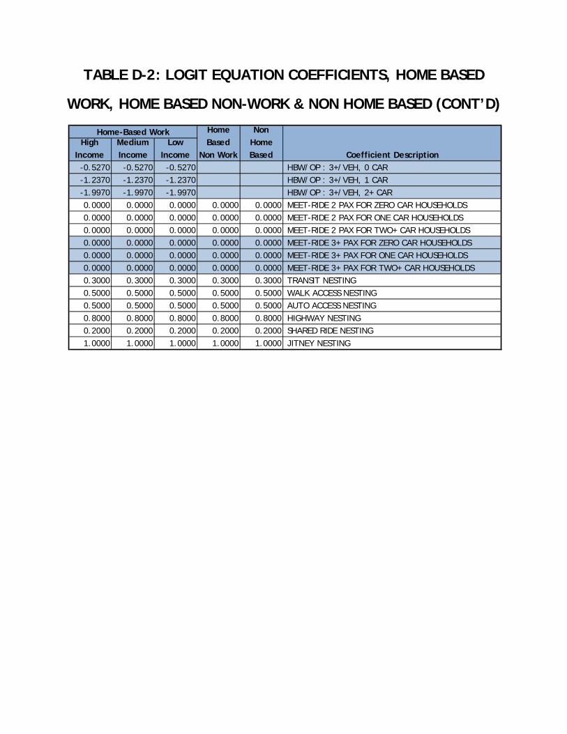
TABLE D-2: LOGIT EQUATION COEFFICIENTS, HOME BASED
WORK, HOME BASED NON-WORK & NON HOME BASED (CONT’D)
-0.5270 -0.5270 -0.5270 HBW/OP : 3+/VEH, 0 CAR -1.2370 -1.2370 -1.2370 HBW/OP : 3+/VEH, 1 CAR -1.9970 -1.9970 -1.9970 HBW/OP : 3+/VEH, 2+ CAR 0.0000 0.0000 0.0000 0.0000 0.0000 MEET-RIDE 2 PAX FOR ZERO CAR HOUSEHOLDS 0.0000 0.0000 0.0000 0.0000 0.0000 MEET-RIDE 2 PAX FOR ONE CAR HOUSEHOLDS 0.0000 0.0000 0.0000 0.0000 0.0000 MEET-RIDE 2 PAX FOR TWO+ CAR HOUSEHOLDS 0.0000 0.0000 0.0000 0.0000 0.0000 MEET-RIDE 3+ PAX FOR ZERO CAR HOUSEHOLDS 0.0000 0.0000 0.0000 0.0000 0.0000 MEET-RIDE 3+ PAX FOR ONE CAR HOUSEHOLDS 0.0000 0.0000 0.0000 0.0000 0.0000 MEET-RIDE 3+ PAX FOR TWO+ CAR HOUSEHOLDS 0.3000 0.3000 0.3000 0.3000 0.3000 TRANSIT NESTING 0.5000 0.5000 0.5000 0.5000 0.5000 WALK ACCESS NESTING 0.5000 0.5000 0.5000 0.5000 0.5000 AUTO ACCESS NESTING 0.8000 0.8000 0.8000 0.8000 0.8000 HIGHWAY NESTING 0.2000 0.2000 0.2000 0.2000 0.2000 SHARED RIDE NESTING 1.0000 1.0000 1.0000 1.0000 1.0000 JITNEY NESTING
Home-Based Work Home Based
Non Work
Non Home Based Coefficient Description
High Income
Medium Income
Low Income
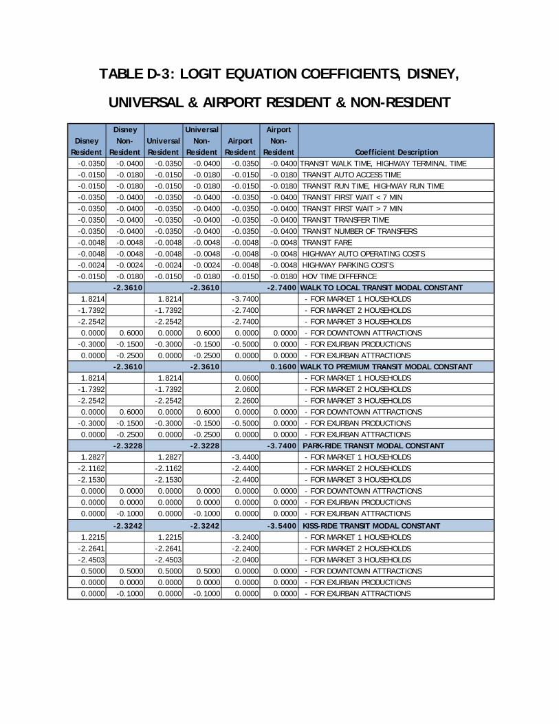
TABLE D-3: LOGIT EQUATION COEFFICIENTS, DISNEY,
UNIVERSAL & AIRPORT RESIDENT & NON-RESIDENT
-0.0350 -0.0400 -0.0350 -0.0400 -0.0350 -0.0400 TRANSIT WALK TIME, HIGHWAY TERMINAL TIME-0.0150 -0.0180 -0.0150 -0.0180 -0.0150 -0.0180 TRANSIT AUTO ACCESS TIME-0.0150 -0.0180 -0.0150 -0.0180 -0.0150 -0.0180 TRANSIT RUN TIME, HIGHWAY RUN TIME-0.0350 -0.0400 -0.0350 -0.0400 -0.0350 -0.0400 TRANSIT FIRST WAIT < 7 MIN-0.0350 -0.0400 -0.0350 -0.0400 -0.0350 -0.0400 TRANSIT FIRST WAIT > 7 MIN-0.0350 -0.0400 -0.0350 -0.0400 -0.0350 -0.0400 TRANSIT TRANSFER TIME -0.0350 -0.0400 -0.0350 -0.0400 -0.0350 -0.0400 TRANSIT NUMBER OF TRANSFERS -0.0048 -0.0048 -0.0048 -0.0048 -0.0048 -0.0048 TRANSIT FARE -0.0048 -0.0048 -0.0048 -0.0048 -0.0048 -0.0048 HIGHWAY AUTO OPERATING COSTS -0.0024 -0.0024 -0.0024 -0.0024 -0.0048 -0.0048 HIGHWAY PARKING COSTS -0.0150 -0.0180 -0.0150 -0.0180 -0.0150 -0.0180 HOV TIME DIFFERNCE
-2.3610 -2.3610 -2.7400 WALK TO LOCAL TRANSIT MODAL CONSTANT1.8214 1.8214 -3.7400 - FOR MARKET 1 HOUSEHOLDS
-1.7392 -1.7392 -2.7400 - FOR MARKET 2 HOUSEHOLDS -2.2542 -2.2542 -2.7400 - FOR MARKET 3 HOUSEHOLDS 0.0000 0.6000 0.0000 0.6000 0.0000 0.0000 - FOR DOWNTOWN ATTRACTIONS
-0.3000 -0.1500 -0.3000 -0.1500 -0.5000 0.0000 - FOR EXURBAN PRODUCTIONS 0.0000 -0.2500 0.0000 -0.2500 0.0000 0.0000 - FOR EXURBAN ATTRACTIONS
-2.3610 -2.3610 0.1600 WALK TO PREMIUM TRANSIT MODAL CONSTANT1.8214 1.8214 0.0600 - FOR MARKET 1 HOUSEHOLDS
-1.7392 -1.7392 2.0600 - FOR MARKET 2 HOUSEHOLDS -2.2542 -2.2542 2.2600 - FOR MARKET 3 HOUSEHOLDS 0.0000 0.6000 0.0000 0.6000 0.0000 0.0000 - FOR DOWNTOWN ATTRACTIONS
-0.3000 -0.1500 -0.3000 -0.1500 -0.5000 0.0000 - FOR EXURBAN PRODUCTIONS 0.0000 -0.2500 0.0000 -0.2500 0.0000 0.0000 - FOR EXURBAN ATTRACTIONS
-2.3228 -2.3228 -3.7400 PARK-RIDE TRANSIT MODAL CONSTANT 1.2827 1.2827 -3.4400 - FOR MARKET 1 HOUSEHOLDS
-2.1162 -2.1162 -2.4400 - FOR MARKET 2 HOUSEHOLDS -2.1530 -2.1530 -2.4400 - FOR MARKET 3 HOUSEHOLDS 0.0000 0.0000 0.0000 0.0000 0.0000 0.0000 - FOR DOWNTOWN ATTRACTIONS 0.0000 0.0000 0.0000 0.0000 0.0000 0.0000 - FOR EXURBAN PRODUCTIONS 0.0000 -0.1000 0.0000 -0.1000 0.0000 0.0000 - FOR EXURBAN ATTRACTIONS
-2.3242 -2.3242 -3.5400 KISS-RIDE TRANSIT MODAL CONSTANT 1.2215 1.2215 -3.2400 - FOR MARKET 1 HOUSEHOLDS
-2.2641 -2.2641 -2.2400 - FOR MARKET 2 HOUSEHOLDS -2.4503 -2.4503 -2.0400 - FOR MARKET 3 HOUSEHOLDS 0.5000 0.5000 0.5000 0.5000 0.0000 0.0000 - FOR DOWNTOWN ATTRACTIONS 0.0000 0.0000 0.0000 0.0000 0.0000 0.0000 - FOR EXURBAN PRODUCTIONS 0.0000 -0.1000 0.0000 -0.1000 0.0000 0.0000 - FOR EXURBAN ATTRACTIONS
Airport Resident
Disney Resident
Disney Non-
Resident
Airport Non-
Resident Coefficient DescriptionUniversal Resident
Universal Non-
Resident

TABLE D-3: LOGIT EQUATION COEFFICIENTS, DISNEY,
UNIVERSAL & AIRPORT RESIDENT & NON-RESIDENT (CONT’D)
0.0000 0.0000 0.0000 ONE PER VEHICLE HIGHWAY MODAL CONSTANT0.0000 0.0000 0.0000 0.0000 - FOR MARKET 1 HOUSEHOLDS 0.0000 0.0000 0.0000 0.0000 - FOR MARKET 2 HOUSEHOLDS 0.0000 0.0000 0.0000 0.0000 - FOR MARKET 3 HOUSEHOLDS 0.0000 0.0000 0.0000 0.0000 - FOR DOWNTOWN ATTRACTIONS
- FOR EXURBAN PRODUCTIONS - FOR EXURBAN ATTRACTIONS
3.7160 3.4650 -0.1400 TWO PER VEHICLE HIGHWAY MODAL CONSTANT1.7500 2.0800 -0.2850 - FOR MARKET 1 HOUSEHOLDS 1.6000 1.9300 -0.3850 - FOR MARKET 2 HOUSEHOLDS 1.3200 1.6500 -0.7850 - FOR MARKET 3 HOUSEHOLDS 0.0000 0.0000 0.0000 0.0000 0.0000 0.0000 - FOR DOWNTOWN ATTRACTIONS
0.0000 0.0000 - FOR EXURBAN PRODUCTIONS 0.0000 0.0000 - FOR EXURBAN ATTRACTIONS
4.2150 3.9490 -0.6430 THREE+ PER VEHICLE HIGHWAY MODAL CONST 2.0700 2.3450 -0.6800 - FOR MARKET 1 HOUSEHOLDS 1.8700 2.1950 -0.8800 - FOR MARKET 2 HOUSEHOLDS 1.3600 1.6350 -1.3800 - FOR MARKET 3 HOUSEHOLDS 0.0000 0.0000 0.0000 0.0000 0.0000 0.0000 - FOR DOWNTOWN ATTRACTIONS
0.0000 0.0000 - FOR EXURBAN PRODUCTIONS 0.0000 0.0000 - FOR EXURBAN ATTRACTIONS
0.3000 0.3000 0.3000 0.3000 0.3000 0.3000 TRANSIT NESTING 0.5000 0.5000 0.5000 0.5000 0.5000 0.5000 WALK ACCESS NESTING 0.5000 0.5000 0.5000 0.5000 0.5000 0.5000 AUTO ACCESS NESTING 0.8000 0.8000 0.8000 0.8000 0.8000 0.8000 HIGHWAY NESTING 0.2000 0.2000 0.2000 0.2000 0.2000 0.2000 SHARED RIDE NESTING 1.0000 1.0000 1.0000 1.0000 1.0000 1.0000 JITNEY NESTING
Airport Resident
Disney Non-
Resident
Airport Non-
Resident Coefficient DescriptionDisney
ResidentUniversal Resident
Universal Non-
Resident

TABLE D-4: LOGIT EQUATION COEFFICIENTS,
ORANGE COUNTY CONVENTION CENTER, SEA WORLD
& I-DRIVE RESIDENT & NON-RESIDENT
-0.0350 -0.0400 -0.0350 -0.0400 -0.0350 -0.0400 TRANSIT WALK TIME, HIGHWAY TERMINAL TIME-0.0150 -0.0180 -0.0150 -0.0180 -0.0150 -0.0180 TRANSIT AUTO ACCESS TIME-0.0150 -0.0180 -0.0150 -0.0180 -0.0150 -0.0180 TRANSIT RUN TIME, HIGHWAY RUN TIME-0.0350 -0.0400 -0.0350 -0.0400 -0.0350 -0.0400 TRANSIT FIRST WAIT < 7 MIN-0.0350 -0.0400 -0.0350 -0.0400 -0.0350 -0.0400 TRANSIT FIRST WAIT > 7 MIN-0.0350 -0.0400 -0.0350 -0.0400 -0.0350 -0.0400 TRANSIT TRANSFER TIME -0.0350 -0.0400 -0.0350 -0.0400 -0.0350 -0.0400 TRANSIT NUMBER OF TRANSFERS -0.0048 -0.0048 -0.0048 -0.0048 -0.0048 -0.0048 TRANSIT FARE -0.0048 -0.0048 -0.0048 -0.0048 -0.0048 -0.0048 HIGHWAY AUTO OPERATING COSTS -0.0024 -0.0024 -0.0024 -0.0024 -0.0024 -0.0024 HIGHWAY PARKING COSTS -0.0150 -0.0180 -0.0150 -0.0180 -0.0150 -0.0180 HOV TIME DIFFERNCE
-2.3610 -2.3610 0.8690 WALK TO LOCAL TRANSIT MODAL CONSTANT1.8214 1.8214 - FOR MARKET 1 HOUSEHOLDS
-1.7392 -1.7392 - FOR MARKET 2 HOUSEHOLDS -2.2542 -2.2542 - FOR MARKET 3 HOUSEHOLDS 0.0000 0.6000 0.0000 0.6000 0.0000 0.0000 - FOR DOWNTOWN ATTRACTIONS
-0.3000 -0.1500 -0.3000 -0.1500 0.0000 0.0000 - FOR EXURBAN PRODUCTIONS 0.0000 -0.2500 0.0000 -0.2500 0.0000 0.0000 - FOR EXURBAN ATTRACTIONS
-2.3610 -2.3610 0.8690 WALK TO PREMIUM TRANSIT MODAL CONSTANT1.8214 1.8214 - FOR MARKET 1 HOUSEHOLDS
-1.7392 -1.7392 - FOR MARKET 2 HOUSEHOLDS -2.2542 -2.2542 - FOR MARKET 3 HOUSEHOLDS 0.0000 0.6000 0.0000 0.6000 0.0000 0.0000 - FOR DOWNTOWN ATTRACTIONS
-0.3000 -0.1500 -0.3000 -0.1500 0.0000 0.0000 - FOR EXURBAN PRODUCTIONS 0.0000 -0.2500 0.0000 -0.2500 0.0000 0.0000 - FOR EXURBAN ATTRACTIONS
-2.3228 -2.3228 0.8690 PARK-RIDE TRANSIT MODAL CONSTANT 1.2827 1.2827 - FOR MARKET 1 HOUSEHOLDS
-2.1162 -2.1162 - FOR MARKET 2 HOUSEHOLDS -2.1530 -2.1530 - FOR MARKET 3 HOUSEHOLDS 0.0000 0.0000 0.0000 0.0000 0.0000 0.0000 - FOR DOWNTOWN ATTRACTIONS 0.0000 0.0000 0.0000 0.0000 0.0000 0.0000 - FOR EXURBAN PRODUCTIONS 0.0000 -0.1000 0.0000 -0.1000 0.0000 0.0000 - FOR EXURBAN ATTRACTIONS
-2.2342 -2.3242 0.8690 KISS-RIDE TRANSIT MODAL CONSTANT 1.2215 1.2215 - FOR MARKET 1 HOUSEHOLDS
-2.2641 -2.2641 - FOR MARKET 2 HOUSEHOLDS -2.4503 -2.4503 - FOR MARKET 3 HOUSEHOLDS 0.5000 0.5000 0.5000 0.5000 0.0000 0.0000 - FOR DOWNTOWN ATTRACTIONS 0.0000 0.0000 0.0000 0.0000 0.0000 0.0000 - FOR EXURBAN PRODUCTIONS 0.0000 -0.1000 0.0000 -0.1000 0.0000 0.0000 - FOR EXURBAN ATTRACTIONS
Coefficient DescriptionOCCC
ResidentOCCC Non-Resident
Sea World Resident
Sea World Non-
ResidentI-Drive
Resident
I-Drive Non-
Resident

TABLE D-4: LOGIT EQUATION COEFFICIENTS,
ORANGE COUNTY CONVENTION CENTER, SEA WORLD
& I-DRIVE RESIDENT & NON-RESIDENT (CONT’D)
0.0000 0.0000 0.0000 ONE PER VEHICLE HIGHWAY MODAL CONSTANT0.0000 0.0000 0.0000 0.0000 0.0000 0.0000 - FOR MARKET 1 HOUSEHOLDS 0.0000 0.0000 0.0000 0.0000 0.0000 0.0000 - FOR MARKET 2 HOUSEHOLDS 0.0000 0.0000 0.0000 0.0000 0.0000 0.0000 - FOR MARKET 3 HOUSEHOLDS 0.0000 0.0000 0.0000 0.0000 0.0000 0.0000 - FOR DOWNTOWN ATTRACTIONS
- FOR EXURBAN PRODUCTIONS - FOR EXURBAN ATTRACTIONS
1.9470 3.4890 0.3790 TWO PER VEHICLE HIGHWAY MODAL CONSTANT1.1020 2.3310 0.3470 - FOR MARKET 1 HOUSEHOLDS 0.9520 2.1810 0.1970 - FOR MARKET 2 HOUSEHOLDS 0.6720 1.9010 -0.0850 - FOR MARKET 3 HOUSEHOLDS 0.0000 0.0000 0.0000 0.0000 0.0000 0.0000 - FOR DOWNTOWN ATTRACTIONS
- FOR EXURBAN PRODUCTIONS - FOR EXURBAN ATTRACTIONS
1.8920 3.5490 0.3580 THREE+ PER VEHICLE HIGHWAY MODAL CONST 0.9390 2.3570 0.2400 - FOR MARKET 1 HOUSEHOLDS 0.7390 2.1570 0.0900 - FOR MARKET 2 HOUSEHOLDS 0.2290 1.6470 -0.4700 - FOR MARKET 3 HOUSEHOLDS 0.0000 0.0000 0.0000 0.0000 0.0000 0.0000 - FOR DOWNTOWN ATTRACTIONS
- FOR EXURBAN PRODUCTIONS - FOR EXURBAN ATTRACTIONS
0.0000 0.0000 0.0000 0.0000 0.0000 0.0000 SUBPURP: 1/VEH, 0 CAR 0.0000 0.0000 0.0000 0.0000 0.0000 0.0000 SUBPURP: 1/VEH, 1 CAR 0.0000 0.0000 0.0000 0.0000 0.0000 0.0000 SUBPURP: 1/VEH, 2+ CAR 0.0000 0.0000 0.0000 0.0000 0.0000 0.0000 SUBPURP: 2/VEH, 0 CAR 0.0000 0.0000 0.0000 0.0000 0.0000 0.0000 SUBPURP: 2/VEH, 1 CAR 0.0000 0.0000 0.0000 0.0000 0.0000 0.0000 SUBPURP: 2/VEH, 2+ CAR 0.0000 0.0000 0.0000 0.0000 0.0000 0.0000 SUBPURP: 3+/VEH, 0 CAR 0.0000 0.0000 0.0000 0.0000 0.0000 0.0000 SUBPURP: 3+/VEH, 1 CAR 0.0000 0.0000 0.0000 0.0000 0.0000 0.0000 SUBPURP: 3+/VEH, 2+ CAR 0.3000 0.3000 0.3000 0.3000 0.3000 0.3000 TRANSIT NESTING 0.5000 0.5000 0.5000 0.5000 0.5000 0.5000 WALK ACCESS NESTING 0.5000 0.5000 0.5000 0.5000 0.5000 0.5000 AUTO ACCESS NESTING 0.8000 0.8000 0.8000 0.8000 0.8000 0.8000 HIGHWAY NESTING 0.2000 0.2000 0.2000 0.2000 0.2000 0.2000 SHARED RIDE NESTING 1.0000 1.0000 1.0000 1.0000 1.0000 1.0000 JITNEY NESTING
Coefficient DescriptionDisney
Resident
Disney Non-
ResidentUniversal Resident
Universal Non-
ResidentAirport
Resident
Airport Non-
Resident

TABLE D-5: TRIP TOTALS FOR HBWRK

TABLE D-6: TRIP TOTALS FOR HBWRK

TABLE D-7: TRIP TOTALS FOR HBWRK

TABLE D-8: TRIP TOTALS FOR HBNWRK
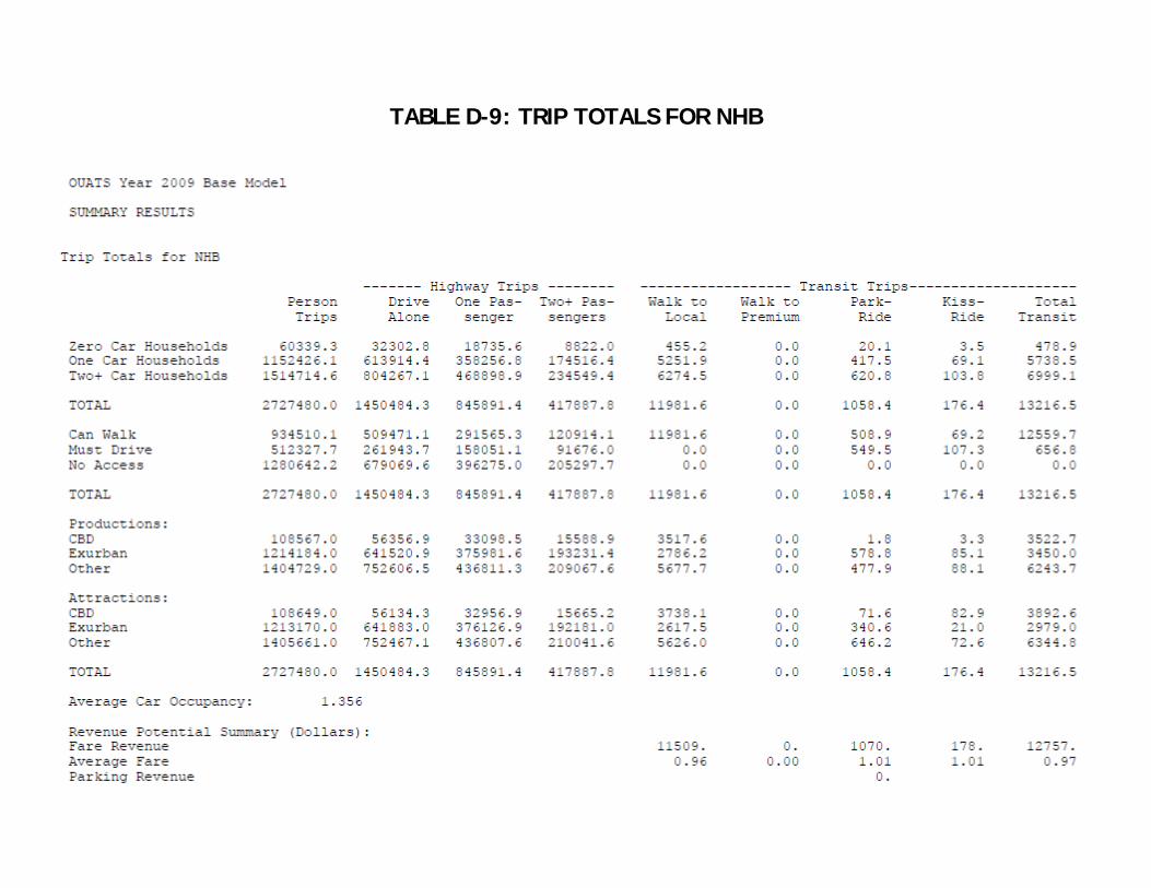
TABLE D-9: TRIP TOTALS FOR NHB

TABLE D-10: TRIP TOTALS FOR TOTNW

TABLE D-11: TRIP TOTALS FOR MCO RES

TABLE D-12: TRIP TOTALS FOR MCO VIS
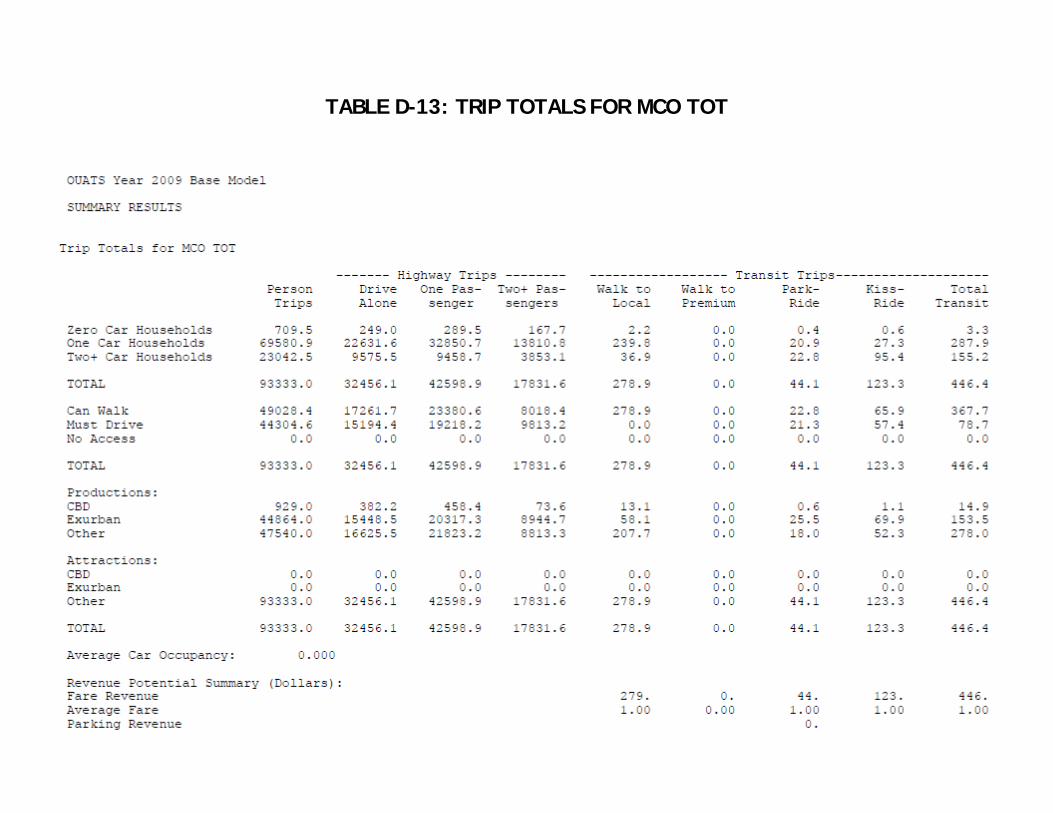
TABLE D-13: TRIP TOTALS FOR MCO TOT

TABLE D-14: TRIP TOTALS FOR OCC RES

TABLE D-15: TRIP TOTALS FOR OCC VIS

TABLE D-16: TRIP TOTALS FOR OCC TOT
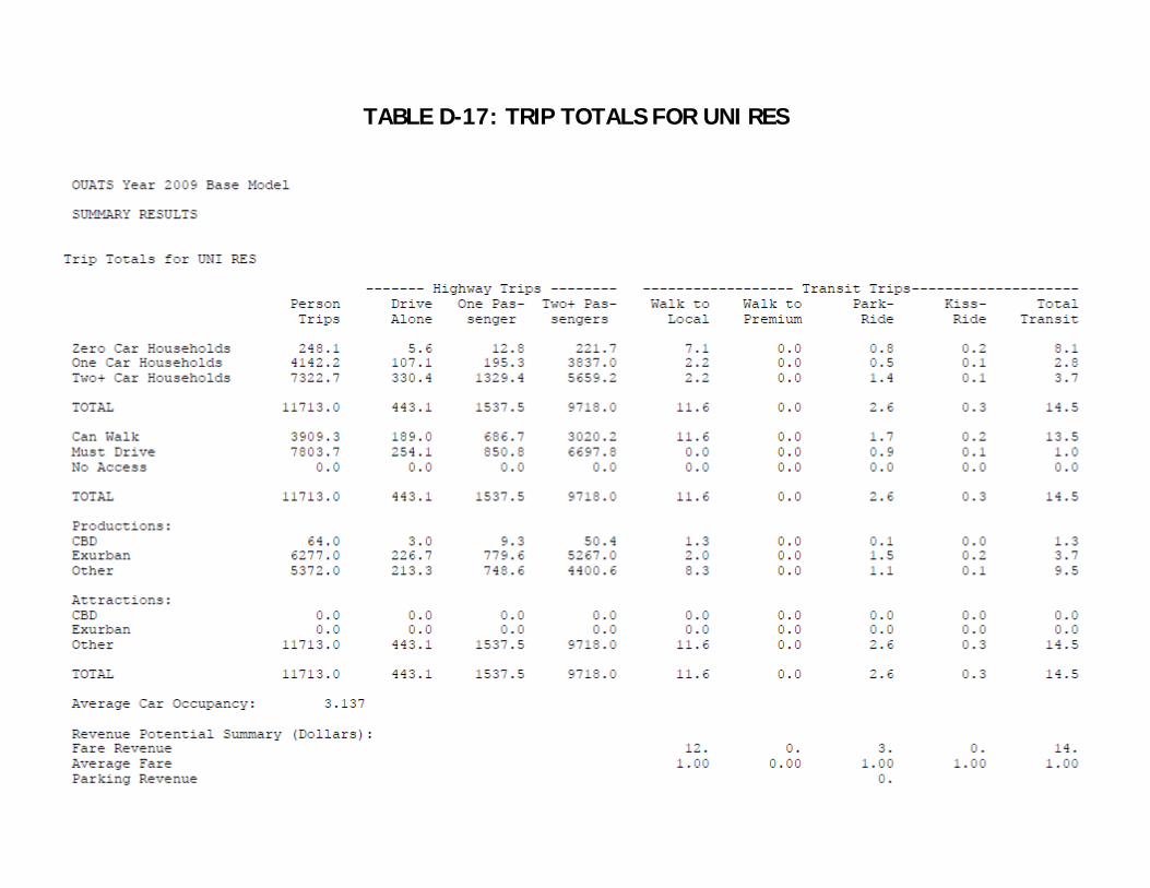
TABLE D-17: TRIP TOTALS FOR UNI RES

TABLE D-18: TRIP TOTALS FOR UNI VIS

TABLE D-19: TRIP TOTALS FOR UNI TOT

TABLE D-20: TRIP TOTALS FOR SEW RES

TABLE D-21: TRIP TOTALS FOR SEW VIS

TABLE D-22: TRIP TOTALS FOR SEW TOT

TABLE D-23: TRIP TOTALS FOR DIS RES
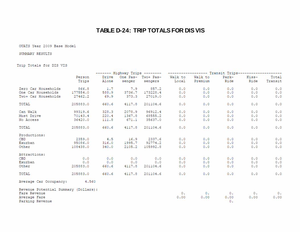
TABLE D-24: TRIP TOTALS FOR DIS VIS
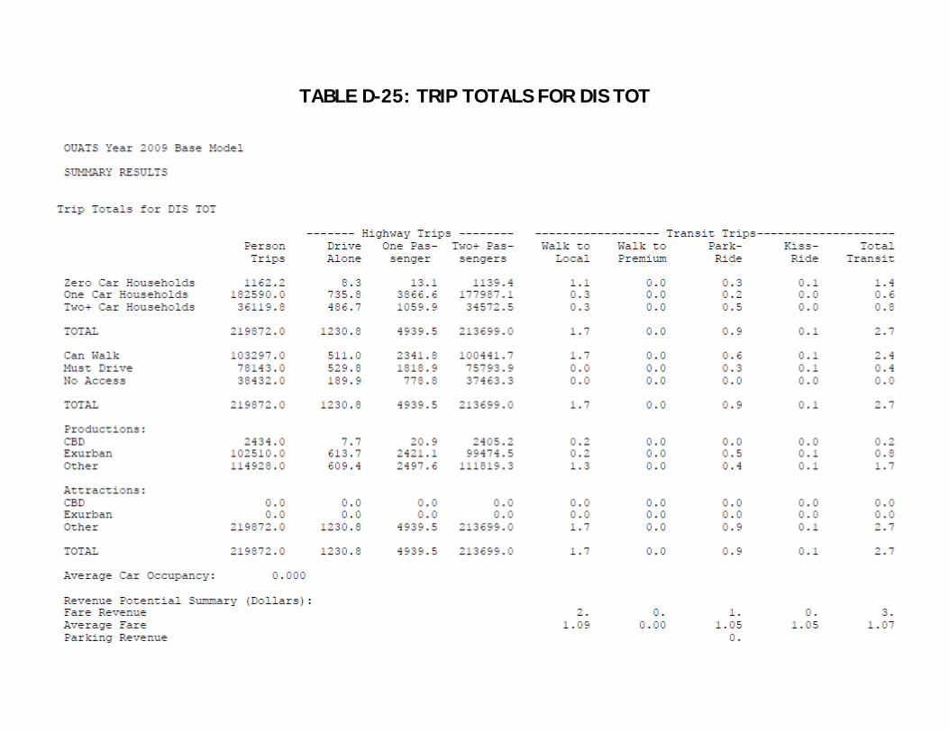
TABLE D-25: TRIP TOTALS FOR DIS TOT

TABLE D-26: TRIP TOTALS FOR IDR RES

TABLE D-27: TRIP TOTALS FOR IDR VIS

TABLE D-28: TRIP TOTALS FOR IDR TOT