technical workgroup #2 - aeso.ca · specifications) and one-off ... turbine model turbine type ......
TRANSCRIPT
Technical Workgroup #2
April 6th, 2018
AESO External
Copyright © 2017 The Brattle Group, Inc.
AESO CONE Study Reference Technology and Financial Assumptions
AESO Technical Working Group Session #2
Michael Hagerty
Mike Tolleth
Hannes Pfeifenberger
Bente Villadsen
The Brattle Group
Ap r i l 6 , 2 0 1 8
P RE S ENTED T O
P RE PARED BY
Sang Gang
Patrick Daou
Sargent & Lundy

| brattle.com 2
Agenda
▀ Project Overview
▀ Screening Analysis and Reference Technology Specifications
▀ Financial Assumptions
▀ Next Steps
| brattle.com 3
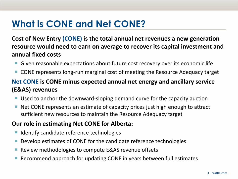
What is CONE and Net CONE?
Cost of New Entry (CONE) is the total annual net revenues a new generation resource would need to earn on average to recover its capital investment and annual fixed costs
▀ Given reasonable expectations about future cost recovery over its economic life
▀ CONE represents long-run marginal cost of meeting the Resource Adequacy target
Net CONE is CONE minus expected annual net energy and ancillary service (E&AS) revenues
▀ Used to anchor the downward-sloping demand curve for the capacity auction
▀ Net CONE represents an estimate of capacity prices just high enough to attract sufficient new resources to maintain the Resource Adequacy target
Our role in estimating Net CONE for Alberta:
▀ Identify candidate reference technologies
▀ Develop estimates of CONE for the candidate reference technologies
▀ Review methodologies to compute E&AS revenue offsets
▀ Recommend approach for updating CONE in years between full estimates

| brattle.com 4
Key Objectives for Estimating Alberta CONE
Provide CONE values for several candidate reference technologies that will allow AESO and its stakeholders to select the appropriate Net CONE value to anchor the demand curve
▀ Reflect the technology, location, and costs that a competitive developer of new generation facilities will be able to achieve at generic sites
▀ Avoid unusual site characteristics (e.g., too tightly defined locations or specifications) and one-off opportunities that are not widely available
▀ Provide relevant research and empirical analysis to inform our recommendations, recognizing where judgments have to made; in such cases, discuss tradeoffs and recommendations for best meeting objectives

| brattle.com 5
CONE Methodology 1) Screen Alberta capacity resources to identify candidate reference technologies
• Reliably able to help meet system load when supply is scarce
• Cost effective as a part of the long-term market equilibrium
• Able to accurately estimate Net CONE
2) Develop detailed specification of reference plants specific to Alberta market • Primarily rely on “revealed preference” of recently developed and proposed plants
• Review environmental regulations, interconnection requirements, fuel supply options
3) Estimate costs to build and operate the specified reference plants • Plant proper capital costs (equipment, materials, labor, EPC contracting costs)
• Owner capital costs (interconnection, startup, land, inventories, financing fees)
• Fixed O&M (labor, materials, property tax, insurance, asset management, working capital)
4) Develop Alberta-specific financial assumptions used to translate costs into CONE • Identify sample of representative companies and estimate their cost of capital
• Consider additional reference points and qualitative risk adjustments
• Select appropriate discount rate for merchant generation
5) Compute CONE for Alberta capacity market • Translate costs into the annualized cost recovery the plant would need to earn based on
its cost recovery path, tax rates, and depreciation schedules over its economic life

| brattle.com 6
Screening Analysis and
Reference Technology Specifications

| brattle.com 7
SCREENING ANALYSIS
Candidates for Alberta Reference Technology
High-level screen ruled out the following as reference technology candidates for Alberta:
▀ Cogeneration and coal-to-gas conversions: significant capacity in Alberta, but non-standard costs and economics; inherent constraints on future capacity
▀ Renewables: not dispatchable resources; built for non-resource adequacy purposes
▀ Energy Storage: costs remain high (~$400-500/kW-yr, but declining); limited capacity deployed
▀ Demand Response: non-standard costs and economics; inherent constraints
Technology
Typical Capacity
(MW)
Alberta Installations
(Planned) since 2008 (MW)
Indicative Plant Capital
Costs* (CAD/kW)
Efficiency (kJ/kWh,
HHV)
Speed of Deployment
(months)
Primary Considerations for Including in Cost
Estimates
Include in Cost
Estimates?
Aero CT 45–115 483
(664) $1,300–2,000
9,200–9,600
20 months Most frequently built
technology
Frame CT 90–370 85
(692) $700–1,850
9,500–11,900
20 months Some recent builds; lowest capital cost
CC 140–850 851
(1,920) $1,200–1,700
6,500–7,800
36 months Most recently installed and planned capacity
Reciprocating Engine (RICE)
30–110 112 (94)
$1,450-1,900 8,800 20 months Limited planned capacity
despite low heat rate and similar capital costs
*Plant costs are high-level estimates intended for screening purposes only. A full bottom-up cost estimate will be used to calculate CONE values. Source: Data downloaded from Ventyx’s Energy Velocity Suite and S&P Global in February 2018, cross referenced with AESO LTA Study
| brattle.com 8
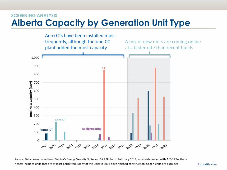
Source: Data downloaded from Ventyx’s Energy Velocity Suite and S&P Global in February 2018, cross referenced with AESO LTA Study.
Notes: Includes units that are at least permitted. Many of the units in 2018 have finished construction. Cogen units are excluded.
SCREENING ANALYSIS
Alberta Capacity by Generation Unit Type
A mix of new units are coming online at a faster rate than recent builds
Aero CTs have been installed most frequently, although the one CC plant added the most capacity

| brattle.com 9
Recently Built and Planned CT Turbines in Alberta
Source: Ventyx’s Energy Velocity Suite and S&P Global in February 2018, cross referenced with AESO LTA Study. Includes units built since 2008 and units that are under construction or permitted .
TECHNOLOGY SPECIFICATON
Turbine Models and Configurations
Simple cycle CTs
▀ LM6000 is the most built turbine type (total capacity and number of units)
▀ Both F-class and E-class frame turbines built − Table does not include turbines
installed for cogen facilities
Combined cycles
▀ Most common CC configuration is 1x1 with H/J-class turbine
▀ CC capacity ranges from 350-850 MW
Recently Built and Planned CC Units in Alberta
Plant Online Year Turbine Model Configuration Capacity
Shepard Energy Centre 2015 Mitsubishi M501G1 2x1 851
Genesee (CAN) 2021 Mitsubishi 501J 1x1 530
Genesee (CAN) 2022 Mitsubishi 501J 1x1 530
Heartland Generating Station 2019 Siemens SGT6-8000H 1x1 510
Saddlebrook Power Station 2021 Siemens SGT6-5000F 1x1 350
Turbine Model Turbine Type
Capacity Installed and
Permitted since 2008
(MW)
Number Installed
and Permitted since
2008
GE LM6000 Aero 719 15
Siemens SGT6-5000F Frame 600 3
GE LMS100 Aero 200 2
Rolls-Royce Trent 60 Aero 198 3
GE 7EA Frame 177 2
Wartsila 18V50SG Reciprocating 94 5
Caterpillar-G16CM34 Reciprocating 65 10
Solar Turbines Inc-Titan 130 Aero 30 2
Cummins C2000 N6C Reciprocating 20 10
Jenbacher JGS 620 Reciprocating 18 6
Wartsila 20V34SG Reciprocating 9 1
Total 2,130 59

| brattle.com 10
TECHNOLOGY SPECIFICATON
Frame CT Turbine Choice
We recommend specifying the F-Class turbine for the frame CT reference technology given its capital cost and efficiency advantages over the E-Class and its smaller size relative to the H-Class.
Consideration Units E-Class F-Class H-Class
Summer Capacity per Turbine
MW 90–115 MW 240 MW 370 MW
Indicative Plant Capital Costs
CAD/kW $1,300–1,850/kW $700-1,100/kW $650-1,000/kW
Efficiency kJ/kWh, HHV 11,500–11,900 10,150 9,500
Alberta Capacity since 2008
Operating MW (Planned MW)
85 MW (92 MW)
0 MW (600 MW)
0 MW (0 MW)
Primary Considerations for Including in Cost Estimates
Smallest capacity and only existing frame CT in Alberta, but high capital
costs and heat rate
Better efficiency and lower capital costs; most
planned in Alberta
Best efficiency and lowest capital costs; none built or planned in Alberta;
much larger than CTs built in Alberta
Include in Cost Estimates?
Source: Data downloaded from Ventyx’s Energy Velocity Suite and S&P Global in February 2018, cross referenced with the AESO LTA Study

| brattle.com 11
TECHNOLOGY SPECIFICATON
Environmental Controls (NOx and CO)
NOx Emissions
▀ Alberta Environment and Parks’ (AEP) current (2005) emissions standards likely require dry low NOx (DLN) burners
▀ AEP is updating standards and is evaluating SCR costs and performance, but has not provided an indication whether new standards will require gas-fired projects to include an SCR
▀ Recent CCs in Alberta have proposed including an SCR (e.g., TransAlta, ATCO); likely being proposed to minimize opposition and project delays related to permitting
CO Emissions
▀ A national source standard of 50 ppm CO was established in 1992
▀ Current CO emissions standard likely will not require oxidation catalyst
Implications for Alberta Reference Technologies
▀ CTs would likely only require DLN burners
▀ CCs would likely include an SCR in anticipation of future NOx regulation and to minimize opposition during permitting, although currently not strictly required

| brattle.com 12
TECHNOLOGY SPECIFICATON
CO2 Emissions Regulations and Turbine Choice
Federal CO2 Emissions Regulations
▀ CO2 limits apply to units with capacity factors (CF) of 33% or greater
▀ Units > 150 MW: 0.42 tons/MWh
▀ Units 25-150 MW: 0.55 tons/MWh
Implications for Alberta Reference Technologies
▀ Aero CTs and CCs are expected to be able to meet their respective emissions limits
▀ Frame CTs will have to operate at less than 33% CF, although historical run times of CTs indicate this limit is not likely to be binding
Alberta’s Carbon Competitiveness Incentive Regulation may further deter higher heat rate CTs from entering the market
| brattle.com 13
TECHNOLOGY SPECIFICATON
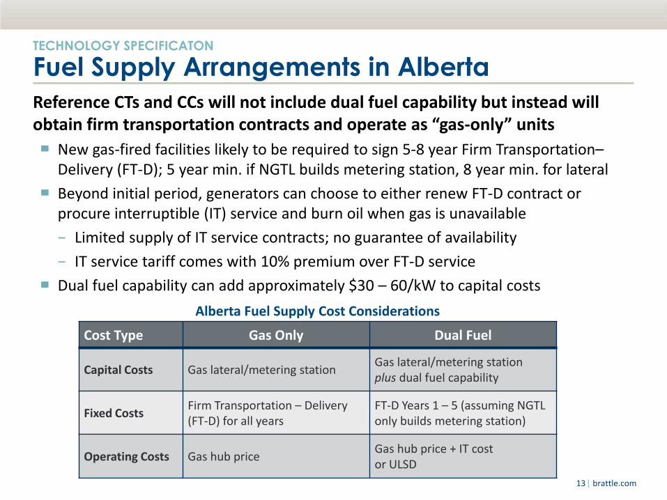
Fuel Supply Arrangements in Alberta
Reference CTs and CCs will not include dual fuel capability but instead will obtain firm transportation contracts and operate as “gas-only” units
▀ New gas-fired facilities likely to be required to sign 5-8 year Firm Transportation–Delivery (FT-D); 5 year min. if NGTL builds metering station, 8 year min. for lateral
▀ Beyond initial period, generators can choose to either renew FT-D contract or procure interruptible (IT) service and burn oil when gas is unavailable
− Limited supply of IT service contracts; no guarantee of availability
− IT service tariff comes with 10% premium over FT-D service
▀ Dual fuel capability can add approximately $30 – 60/kW to capital costs
Cost Type Gas Only Dual Fuel
Capital Costs Gas lateral/metering station Gas lateral/metering station plus dual fuel capability
Fixed Costs Firm Transportation – Delivery (FT-D) for all years
FT-D Years 1 – 5 (assuming NGTL only builds metering station)
Operating Costs Gas hub price Gas hub price + IT cost or ULSD
Alberta Fuel Supply Cost Considerations
| brattle.com 14
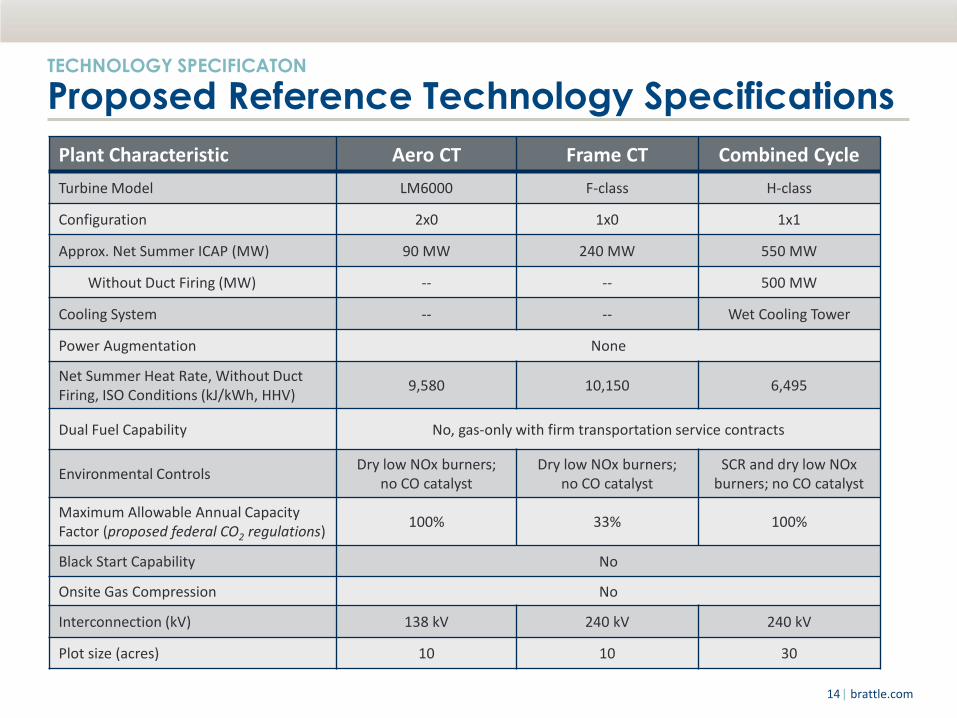
Plant Characteristic Aero CT Frame CT Combined Cycle
Turbine Model LM6000 F-class H-class
Configuration 2x0 1x0 1x1
Approx. Net Summer ICAP (MW) 90 MW 240 MW 550 MW
Without Duct Firing (MW) -- -- 500 MW
Cooling System -- -- Wet Cooling Tower
Power Augmentation None
Net Summer Heat Rate, Without Duct Firing, ISO Conditions (kJ/kWh, HHV)
9,580 10,150 6,495
Dual Fuel Capability No, gas-only with firm transportation service contracts
Environmental Controls Dry low NOx burners;
no CO catalyst Dry low NOx burners;
no CO catalyst SCR and dry low NOx
burners; no CO catalyst
Maximum Allowable Annual Capacity Factor (proposed federal CO2 regulations)
100% 33% 100%
Black Start Capability No
Onsite Gas Compression No
Interconnection (kV) 138 kV 240 kV 240 kV
Plot size (acres) 10 10 30
TECHNOLOGY SPECIFICATON
Proposed Reference Technology Specifications

| brattle.com 15
Edmonton
Both Edmonton and Calgary are potential locations for development with limited cost variation between the two
Note: ST units are coal units scheduled to retire 2019-2025.
LOCATIONAL ANALYSIS
Alberta Reference Location
Calgary
▀ Recent Gas Builds: Majority of gas plants are located near Calgary and Edmonton
▀ Interconnection: Gas and electric infrastructure available in both locations
▀ Labor Costs: Crew rates in Calgary and Edmonton are comparable; labor costs will not be major driver of location
▀ Permitting: Water supply may be an issue in the Calgary area
▀ Losses Factors: Similar, average is slightly higher in Edmonton than Calgary
▀ Ambient Conditions: Similar temp, relative humidity; lower elevation in Edmonton
Recommend the region around Edmonton for bottom-up cost estimates
Gas pipelines
Transmission

| brattle.com 16
Next Steps: Plant Capital Cost Estimates
Major Equipment
▀ Current major OEM pricing in Alberta, validate OEM pricing against market trends
▀ Internal database of major BOP components for remainder of pricing
Labor
▀ Labor rates will reflect Edmonton labor pools as well as applicable overhead costs
▀ Per diem added if the site is considered remote or quantity of local labor is not sufficient
▀ Labor hours and productivity will be reflective of the local labor pools
Balance of Plant, Materials, & Commodities
▀ High level design to account for all the major systems required for plant operation
▀ Material and commodity quantities to match the BOP design
▀ BOP design will take into account site specific conditions, i.e. greenfield/brownfield, location ambient conditions, etc.
Owner’s Development Costs
▀ Development, testing/startup, non-fuel inventories based on internal database
▀ Land, net startup fuel costs, and fuel inventories rely on local Edmonton market conditions
▀ Gas/electric interconnection costs based on recently observed project costs

| brattle.com 17
Financial Assumptions

| brattle.com 18
FINANCIAL ASSUMPTIONS
Cost of Capital Principles for CONE Discount Rate
Forward-looking opportunity cost of capital appropriate to the risk of the enterprise being contemplated:
▀ Development and operation of green-field gas-fired generating plant in Alberta
▀ Revenue from merchant sales into Alberta wholesale market—not PPA contracted capacity—since…
− PPA transfers market risk from generator to counterparty
− Capacity market is intended to attract investment without bilateral contracting
After-tax Weighted Average Cost of Capital (ATWACC)
▀ Represents total after-tax cost of financing:
𝐴𝑇𝑊𝐴𝐶𝐶 = %𝐸 × 𝑟𝐸 + %𝐷 × 𝑟𝐷 × (1 − 𝑡)
▀ Appropriate formulation for discounting unlevered free cash flows (which CONE calculation does to annualize plant costs)
▀ Independent of specific financing over a broad middle range of capital structures
− Recognizes that required return on equity increases with financial risk of additional debt leverage

| brattle.com 19
Overall Cost of Capital and Its Components
FINANCIAL ASSUMPTIONS
Approach to Estimating Alberta Cost of Capital
Public Sample Companies • Risk-appropriate proxy groups • Estimate ATWACC from market data • Forward-looking inputs as of 2018
Recent IPP Transactions • Discount rates (ATWACC) used for
valuations (fairness opinions) • Adjust for changes in market conditions
Range of Risk-Appropriate ATWACC Estimates
for Merchant Operations
Alberta-Specific ATWACC
Cost of Equity
Cost of Debt
Debt-to-Equity Ratio
Internally Consistent Financing Components
Qualitative Risk Assessment
| brattle.com 20
FINANCIAL ASSUMPTIONS
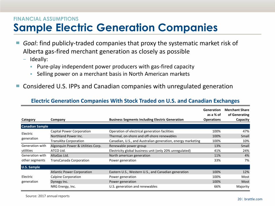
Sample Electric Generation Companies
▀ Goal: find publicly-traded companies that proxy the systematic market risk of Alberta gas-fired merchant generation as closely as possible − Ideally:
Pure-play independent power producers with gas-fired capacity Selling power on a merchant basis in North American markets
▀ Considered U.S. IPPs and Canadian companies with unregulated generation
Electric Generation Companies With Stock Traded on U.S. and Canadian Exchanges
Source: 2017 annual reports
Category Company Business Segments Including Electric Generation
Generation
as a % of
Operations
Merchant Share
of Generating
Capacity
Canadian Sample
Capital Power Corporation Operation of electrical generation facilities 100% 47%
Northland Power Inc. Thermal, on-shore and off-shore renewables 100% Small
TransAlta Corporation Canadian, U.S., and Australian generation, energy marketing 100% 10%
Algonquin Power & Utilities Corp. Renewable power group 13% Small
ATCO Ltd. Electricity global business unit (only 20% unregulated) 41% 24%
AltaGas Ltd. North american generation 11% 4%
TransCanada Corporation Power generation 33% 7%
U.S. Sample
Atlantic Power Corporation Eastern U.S., Western U.S., and Canadian generation 100% 12%
Calpine Corporation Power generation 100% Most
Dynegy Inc. Power generation 100% Most
NRG Energy, Inc. U.S. generation and renewables 66% Majority
Electric
generation
Generation with
utilities
Generation with
other segments
Electric
generation
| brattle.com 21
FINANCIAL ASSUMPTIONS
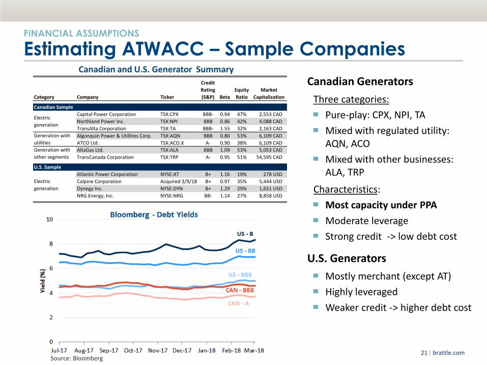
Estimating ATWACC – Sample Companies
Canadian Generators
Three categories:
▀ Pure-play: CPX, NPI, TA
▀ Mixed with regulated utility: AQN, ACO
▀ Mixed with other businesses: ALA, TRP
Characteristics:
▀ Most capacity under PPA
▀ Moderate leverage
▀ Strong credit -> low debt cost
U.S. Generators
▀ Mostly merchant (except AT)
▀ Highly leveraged
▀ Weaker credit -> higher debt cost
Canadian and U.S. Generator Summary
Source: Bloomberg
Category Company Ticker
Credit
Rating
(S&P) Beta
Equity
Ratio
Market
Capitalization
Canadian Sample
Capital Power Corporation TSX:CPX BBB- 0.94 47% 2,553 CAD
Northland Power Inc. TSX:NPI BBB 0.86 42% 4,088 CAD
TransAlta Corporation TSX:TA BBB- 1.55 32% 2,163 CAD
Algonquin Power & Utilities Corp. TSX:AQN BBB 0.80 53% 6,109 CAD
ATCO Ltd. TSX:ACO.X A- 0.90 38% 6,109 CAD
AltaGas Ltd. TSX:ALA BBB 1.09 53% 5,053 CAD
TransCanada Corporation TSX:TRP A- 0.95 51% 54,595 CAD
U.S. Sample
Atlantic Power Corporation NYSE:AT B+ 1.16 19% 278 USD
Calpine Corporation Acquired 3/9/18 B+ 0.97 35% 5,444 USD
Dynegy Inc. NYSE:DYN B+ 1.29 29% 1,651 USD
NRG Energy, Inc. NYSE:NRG BB- 1.14 27% 8,858 USD
Electric
generation
Generation with
utilities
Generation with
other segments
Electric
generation

| brattle.com 22
FINANCIAL ASSUMPTIONS
Estimating ATWACC – Sample Companies
Canadian and U.S. Samples
▀ Canadian generators mostly earn revenue under long-term PPA contracts
− Company composition fairly stable
− Some have unregulated generation integrated with other business segments
▀ U.S electric generator sample is characterized by greater degree of merchant sales into wholesale power markets
− Relatively “pure play” independent power producers
− Few companies, frequent M&A activity, and some bankruptcies
▀ Directionally, we believe U.S. IPPs have higher systematic risk, but neither group may fully capture risk of merchant gas-fired generation in Alberta power market
Stock Prices of Canadian Generator Sample
Stock Prices of U.S. Generator Sample
Source: Bloomberg

| brattle.com 23
FINANCIAL ASSUMPTIONS
Estimating ATWACC – Transaction Benchmarks
Discount Rates Applied in Transaction Proxy Statements
Source: SEC DEFM14A Proxy Statements Notes: Talen Proxy Statement range includes valuations from January 2016 as well as May/June 2016. Forward-looking adjustments based on changes in risk-free rate: U.S. 20-yr T-bond yields were 2.6% in both January 2016 and January 2018, and 2.2% in June 2016; current yields are 3.0% and forecasts 4.2% for 2022.
Discount Rates Used in Recent Generation Asset Transactions ▀ U.S. M&A transactions are accompanied by Proxy Statements, which include
valuations, often performed by discounting projected cash flows at the ATWACC
− Assumptions underlying the ATWACC calculation are not typically explained
− Transaction proxy statements are a reference point to help benchmark the cost of capital
▀ We view three recent/ongoing acquisitions in the U.S. IPP space as relevant
− Talen, a public company that controlled 16,000 MWs of capacity, was acquired by the private company Riverstone Holdings in 2016
− Calpine, a public company that owned 26,000 MWs of capacity, was acquired by Energy Capital Partners and a consortium of other private investors (closed in 2018)
− Dynegy, a public company that owns 22,000 MW of capacity, is being acquired by Vistra
Announce
Date Close Date Buyer Target Valuation Date
Stated Discount
Rate Range
(ATWACC)
Adjusted Forward-
Looking Range
30-Oct-2017 ongoing Vistra Energy Dynegy 01-Jan-2018 4.6% - 7.7% 5.9% - 9.0%
18-Aug-2017 08-Mar-2018 Energy Capital Partners Calpine 01-Jun-2017 5.75% - 6.25% 7.1% - 7.6%
03-Jun-2016 06-Dec-2016 Riverstone Holdings Talen 02-Jun-2016 5.9% - 7.3% 7.6% - 8.6%

| brattle.com 24
FINANCIAL ASSUMPTIONS
Reference Point Sample: Oil Sands Companies
Alternative Sample – Canadian Oil Sands
▀ Brattle is also investigating as a reference point a sample of petroleum producers with operations focused in the Alberta oil sands.
▀ Characteristics: low leverage / strong credit, but high systematic equity risk
Stock Price History
Canadian Oil Sands Sample
Spot Crude and Power Prices
Sources: Bloomberg, Ventyx
Company Ticker
Credit
Rating
(S&P) Beta
Equity
Ratio
Market
Capitalization
(CAD)
Canadian Natural Resources Limited TSX:CNQ BBB+ 1.78 73% 53,910
Cenovus Energy Inc. TSX:CVE BBB 1.45 73% 14,138
Husky Energy Inc. TSX:HSE BBB+ 1.39 77% 16,862
Imperial Oil Limited TSX:IMO AA+ 1.08 87% 32,182
Suncor Energy Inc. TSX:SU A- 1.18 80% 73,247
| brattle.com 25
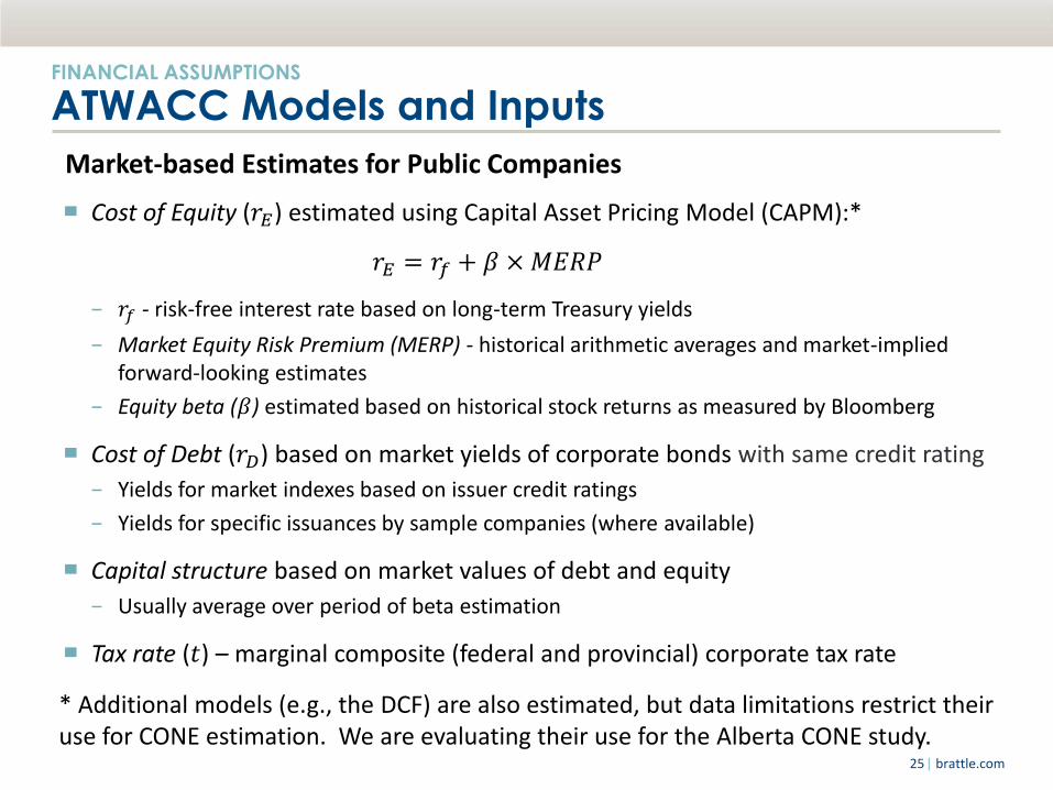
FINANCIAL ASSUMPTIONS
ATWACC Models and Inputs
Market-based Estimates for Public Companies
▀ Cost of Equity (𝑟𝐸) estimated using Capital Asset Pricing Model (CAPM):*
𝑟𝐸 = 𝑟𝑓 + 𝛽 × 𝑀𝐸𝑅𝑃
− 𝑟𝑓 - risk-free interest rate based on long-term Treasury yields
− Market Equity Risk Premium (MERP) - historical arithmetic averages and market-implied forward-looking estimates
− Equity beta (𝛽) estimated based on historical stock returns as measured by Bloomberg
▀ Cost of Debt (𝑟𝐷) based on market yields of corporate bonds with same credit rating
− Yields for market indexes based on issuer credit ratings
− Yields for specific issuances by sample companies (where available)
▀ Capital structure based on market values of debt and equity
− Usually average over period of beta estimation
▀ Tax rate (𝑡) – marginal composite (federal and provincial) corporate tax rate
* Additional models (e.g., the DCF) are also estimated, but data limitations restrict their use for CONE estimation. We are evaluating their use for the Alberta CONE study.

| brattle.com 26
FINANCIAL ASSUMPTIONS
Cost of Equity Inputs
Canadian and U.S. Treasury Bonds Market Equity Risk Premium
Risk-free rate and Market Equity Risk Premium (MERP)
▀ We analyzed Canadian and U.S. 20-year government bond yields:
− 3.8% and 4.2%, respectively, by the end of 2022
▀ We use MERP of 7%, which is broadly consistent with historical and forward-looking (market-implied) estimates for Canada and the U.S.
Historical
Average MERP
Current
Market
Implied MERP
[1] [2]
Canada 5.7% 9.0%
U.S. 6.9% 6.8%
[2]: Bloomberg; adjusted to be expressed
relative to 20-year T-bond yield.
[1]: Duff and Phelps, International Guide to
the Cost of Capital, 2017. 1926-2016 for U.S.;
1935-2016 for Canada

| brattle.com 27
FINANCIAL ASSUMPTIONS
Cost of Debt Inputs
Corporate Bond Yields
▀ We analyzed yields from 20-year Canadian and U.S. corporate bond indexes to infer marginal cost of debt
− Match sample companies’ issuer ratings to the ratings range of the index
− Forward-looking adjustments made to reflect forecast rising interest rates
▀ Also researching yields on company-specific bond issues, which may differ Canadian and U.S. Corporate Bond Index Yields
Source: Bloomberg

| brattle.com 28
FINANCIAL ASSUMPTIONS
Financing New Power Generation Projects Capital required to fund new generation projects is typically a combination of equity
investments and debt financing. The debt can be financed in two ways: ▀ Project financing (non-recourse financing)
− Debt is repaid strictly through project revenues; in the event of insolvency, lenders can only recover their investment from the project itself
− Higher costs due to higher risk of default; exposure to transitory periods of cash flow shortfall from merchant operations in volatile markets
− Despite high cost, may be attractive to developers as the only source of available financing or because it limits the equity investor’s risk to initial equity investment
− Generally requires long-term PPAs because lenders must be confident in project’s revenue stream in order to accept the higher risk of default
▀ Balance sheet financing − Debt is funded with recourse to owner/developer’s entire balance sheet − Greater certainty for lenders; repayment tied to solvency of a large, diversified company − Requires investors with sufficient scale and diversification, but increases financing opportunities
for merchant generation projects without PPAs
Our CONE estimates will rely on balance sheet financing, because ▀ The discount rate used to translate costs into CONE should depend on project risk, not the method
of financing ▀ When available, balance sheet financing is generally lower cost than project financing ▀ The Alberta market, like other deregulated power markets, does not support investment cost
recovery through long-term PPAs (as would be required to obtain project financing); suppliers must bear the risk that a particular investment will be uneconomic. This makes Alberta unattractive to investors who typically provide project-financing.
| brattle.com 29
FINANCIAL ASSUMPTIONS
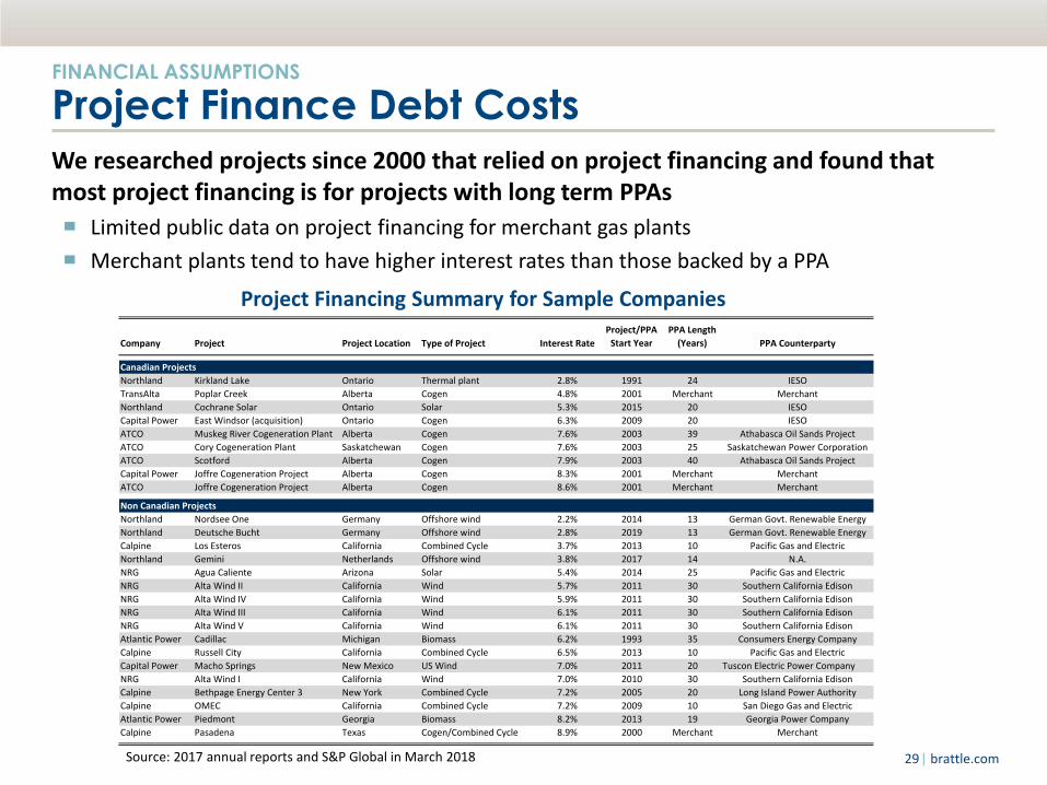
Project Finance Debt Costs
We researched projects since 2000 that relied on project financing and found that most project financing is for projects with long term PPAs
▀ Limited public data on project financing for merchant gas plants
▀ Merchant plants tend to have higher interest rates than those backed by a PPA
Source: 2017 annual reports and S&P Global in March 2018
Company Project Project Location Type of Project Interest Rate
Project/PPA
Start Year
PPA Length
(Years) PPA Counterparty
Canadian Projects
Northland Kirkland Lake Ontario Thermal plant 2.8% 1991 24 IESO
TransAlta Poplar Creek Alberta Cogen 4.8% 2001 Merchant Merchant
Northland Cochrane Solar Ontario Solar 5.3% 2015 20 IESO
Capital Power East Windsor (acquisition) Ontario Cogen 6.3% 2009 20 IESO
ATCO Muskeg River Cogeneration Plant Alberta Cogen 7.6% 2003 39 Athabasca Oil Sands Project
ATCO Cory Cogeneration Plant Saskatchewan Cogen 7.6% 2003 25 Saskatchewan Power Corporation
ATCO Scotford Alberta Cogen 7.9% 2003 40 Athabasca Oil Sands Project
Capital Power Joffre Cogeneration Project Alberta Cogen 8.3% 2001 Merchant Merchant
ATCO Joffre Cogeneration Project Alberta Cogen 8.6% 2001 Merchant Merchant
Non Canadian Projects
Northland Nordsee One Germany Offshore wind 2.2% 2014 13 German Govt. Renewable Energy
Northland Deutsche Bucht Germany Offshore wind 2.8% 2019 13 German Govt. Renewable Energy
Calpine Los Esteros California Combined Cycle 3.7% 2013 10 Pacific Gas and Electric
Northland Gemini Netherlands Offshore wind 3.8% 2017 14 N.A.
NRG Agua Caliente Arizona Solar 5.4% 2014 25 Pacific Gas and Electric
NRG Alta Wind II California Wind 5.7% 2011 30 Southern California Edison
NRG Alta Wind IV California Wind 5.9% 2011 30 Southern California Edison
NRG Alta Wind III California Wind 6.1% 2011 30 Southern California Edison
NRG Alta Wind V California Wind 6.1% 2011 30 Southern California Edison
Atlantic Power Cadillac Michigan Biomass 6.2% 1993 35 Consumers Energy Company
Calpine Russell City California Combined Cycle 6.5% 2013 10 Pacific Gas and Electric
Capital Power Macho Springs New Mexico US Wind 7.0% 2011 20 Tuscon Electric Power Company
NRG Alta Wind I California Wind 7.0% 2010 30 Southern California Edison
Calpine Bethpage Energy Center 3 New York Combined Cycle 7.2% 2005 20 Long Island Power Authority
Calpine OMEC California Combined Cycle 7.2% 2009 10 San Diego Gas and Electric
Atlantic Power Piedmont Georgia Biomass 8.2% 2013 19 Georgia Power Company
Calpine Pasadena Texas Cogen/Combined Cycle 8.9% 2000 Merchant Merchant
Project Financing Summary for Sample Companies

| brattle.com 30
Next Steps
▀ Finalize candidate Alberta reference technology specifications
▀ Develop bottom-up cost estimates
▀ Calculate and finalize recommended ATWACC for Alberta generation investment
▀ Apply financial model to calculate CONE
▀ Review Alberta net E&AS revenue methodologies
Stakeholder Meeting Schedule
▀ May: Provide progress update
▀ June: Present draft CONE results
Next Steps and Schedule
| brattle.com 31
Appendix

| brattle.com 32
Alberta Capacity by Gen Type
Note: This includes natural gas fired units in Alberta All of these units through 2017 are operating, as well as some in 2018. All of the units starting in 2018 are at least permitted. If CT units did not include a turbine type to identify the type, the following assumptions were made: 15 - 110 MWs were aero and greater than 110 MWs were frame type.
Source: Data downloaded from Ventyx’s Energy Velocity Suite and S&P Global in February 2018, cross referenced with the AESO Long Term Adequacy Study
Capacity Count
Year CC Frame CT Aero CT RICE Cogen CC Frame CT Aero CT RICE Cogen
2008 0 85 90 0 0 0 1 2 0 0
2009 0 0 220 0 0 0 0 4 0 0
2010 0 0 100 0 151 0 0 1 0 3
2011 0 0 0 0 50 0 0 0 0 1
2012 0 0 0 1 133 0 0 0 1 2
2013 0 0 0 0 85 0 0 0 0 1
2014 0 0 30 74 0 0 0 2 11 0
2015 851 0 0 37 285 1 0 0 15 4
2016 0 0 0 0 0 0 0 0 0 0
2017 0 0 0 0 0 0 0 0 0 0
2018 0 92 329 0 380 0 1 5 0 2
2019 510 0 0 0 214 1 0 0 0 4
2020 0 600 180 94 96 0 3 4 5 2
2021 880 0 198 0 540 2 0 3 0 6
2022 530 0 0 0 35 1 0 0 0 1
Total Existing 851 85 440 112 703 1 1 9 27 11
Average Existing MW 851 85 49 4 64
Total Planned 1,920 692 707 94 1,265 4 4 12 5 15
Average Planned MW 480 173 59 0 84

| brattle.com 33
Comparison of Alberta to Rest of Canada
Source: Data downloaded from Ventyx’s Energy Velocity Suite in February 2018.
Note: This includes all recently built, natural gas-fired units in Alberta and the rest of Canada, 2008-2017.
New Natural Gas-Fired Capacity in Alberta and the Rest of Canada, 2008-2017
Alberta Capacity Rest of Canada Capacity Rest of Canada Count
Year CC Frame CT Aero CT RICE Cogen CC > 110 MW CT 15-110 MW CT RICE
2008 0 85 90 0 0 1,588 330 0 25
2009 0 0 220 0 0 1,515 0 178 0
2010 0 0 100 0 151 948 0 237 0
2011 0 0 0 0 50 0 0 86 0
2012 0 0 0 1 133 174 393 0 26
2013 0 0 0 0 85 261 0 0 0
2014 0 0 30 74 0 0 0 0 0
2015 851 0 0 37 285 205 0 0 0
2016 0 0 0 0 0 0 0 0 0
2017 0 0 0 0 0 296 0 0 0
Total 851 85 440 112 703 4,987 723 501 50
Average MW 851 85 49 4 64 453 181 42 10

| brattle.com 34
Alberta Oil Sands Business Segments
Company Business Segments Including Oil Sands
Oil sands as
a % of
Revenues
Canadian Natural Resources Limited Oil sands mining and upgrading 25%
Cenovus Energy Inc. Oil sands; deep basin development 45%
Husky Energy Inc. Upstream: exploration, production, infrastructure and marketing 36%
Imperial Oil Limited Upstream (production for sale) 31%
Suncor Energy Inc. Oil sands mining and in situ 40%
Alberta Oil Sand Production Companies With Stock Traded on U.S. and Canadian Exchanges
Source: 2016 and 2017 annual reports

Resource Adequacy Modeling
Technical Workgroup #2
April 6th, 2018 AESO External

Technical Workgroup Objective: AESO
Resource Adequacy Model
• Through the WG process seeking workgroup members
review and provide input on the methodology, key inputs and
outputs of the AESO resource adequacy modeling that will
determine the amount of capacity required to meet the
defined reliability target.
– Through the review feedback and acceptance will be sought
from the workgroup to validate that the AESO is using:
• Reasonable assumptions and methodologies
• Clear transparent process
• Industry standard practices
Today we will review the Resource Adequacy Model (RAM),
specifically the outstanding inputs from the 2017 discussion
and review preliminary draft results.
36

Revised Agenda
For Discussion:
• Astrapé, SERVM and the Model Mechanics
• Thermal
– Maintenance, Forced Outage, Seasonal Derates
• Cogeneration
• Emergency Operations/Ancillary Services
• Draft - Results
– Reserve Margin
– Reference Technology
– Draft Result
– Sensitivities
• Next Steps
For Information:
• Demand
– Weather/Economic
• Intertie
• Renewable
– Wind, Solar, Hydro

Material for Discussion

Astrapé, SERVM and the Model Mechanics
• AESO has procured the Strategic Energy and Risk Valuation Model (SERVM)
which is managed by Astrapé Consulting
– SERVM was developed in 2005
– Astrapé has extensive experience in resource adequacy modeling, assessing
physical reliability metrics as well as capturing economic metrics for regulated
utilities, regulators, and independent system operators.
– Clients include CPUC, ERCOT, SPP, Southern Company, PJM and MISO
and FERC
• The tool allows for fast simulation of thousands of iterations of unit performance to
identify frequency and magnitude of firm load shed events.
– Hourly chronological dispatch
– Stochastic (Monte Carlo) simulation
– Distribution for load/weather, load growth uncertainty, outages, intermittent
renewable output, intertie, and emergency operating procedures

Astrapé, SERVM and the Model Mechanics
• Construction of Scenarios: after a resource mix is defined
SERVM runs 7,500 different 8,760 hour simulations
– 30 Weather years (Load and Renewable profiles)
– Load forecast error (Distribution of 5 points)
– Unit outage modeling, capturing frequency and duration
(50 iterations)

Thermal – Planned Maintenance
• The maintenance scheduling algorithm in Resource Adequacy Model (RAM) is to
schedule maintenance events such that each event scheduled impacts the lowest
load days possible.
• The algorithm is based on daily peak loads, thus placing significant maintenance
events in the spring and fall based on lower loads in those periods.
– Historical Available Capacity (AC) data (2015-2016) was used to analyze
planned maintenance.
• While the maintenance patterns vary from year-to-year for individual generators,
the aggregate MWh on maintenance for the entire system is relatively stable thus
2 years is a reasonable proxy for maintenance events
– For non-coal units that were missing data, a 2% maintenance rate was
entered
– As the outage scheduling algorithm doesn't account for lower cogeneration
output in the shoulder season, some maintenance events were manually
scheduled and placed in the summer as to not exacerbate reliability issues.
AESO External
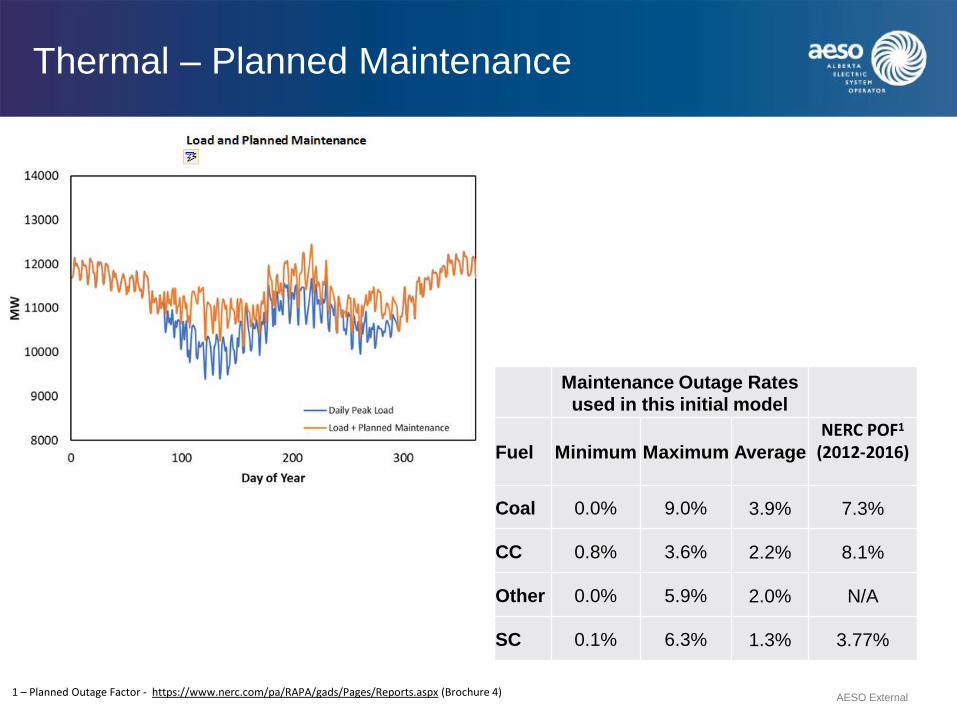
Thermal – Planned Maintenance
Maintenance Outage Rates
used in this initial model
Fuel Minimum Maximum Average NERC POF1
(2012-2016)
Coal 0.0% 9.0% 3.9% 7.3%
CC 0.8% 3.6% 2.2% 8.1%
Other 0.0% 5.9% 2.0% N/A
SC 0.1% 6.3% 1.3% 3.77%
AESO External
1 – Planned Outage Factor - https://www.nerc.com/pa/RAPA/gads/Pages/Reports.aspx (Brochure 4)

Thermal – Forced Outage
• A distribution of time-to-fail hours (TTF) and time-to-repair
(TTR) hours were calculate for each unit to ensure that
historical EFOR is captured in the model.
– The model used historical thermal Energy Trading System
(ETS) data from 2012-2017 to identify forced outage and forced
derate events
– Identified planned outage events are excluded
– Units were referenced to other units in the same unit type if
they did not have sufficient historical statistics available
• RAM then randomly draws from these events to simulate the
unit forced outage events
43 AESO External
Thermal – Forced Outage
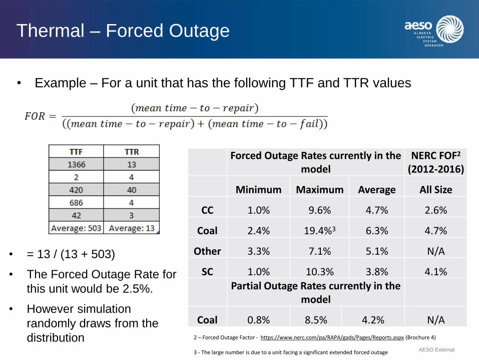
• Example – For a unit that has the following TTF and TTR values
• = 13 / (13 + 503)
• The Forced Outage Rate for
this unit would be 2.5%.
• However simulation
randomly draws from the
distribution
Forced Outage Rates currently in the model
NERC FOF2 (2012-2016)
Minimum Maximum Average All Size
CC 1.0% 9.6% 4.7% 2.6%
Coal 2.4% 19.4%3 6.3% 4.7%
Other 3.3% 7.1% 5.1% N/A
SC 1.0% 10.3% 3.8% 4.1% Partial Outage Rates currently in the
model
Coal 0.8% 8.5% 4.2% N/A
AESO External
2 – Forced Outage Factor - https://www.nerc.com/pa/RAPA/gads/Pages/Reports.aspx (Brochure 4)
3 - The large number is due to a unit facing a significant extended forced outage

Thermal – Seasonal Derates
• Technology output curves were used to model weather related derates for
Combined Cycle and Simple Cycle units
• The technology output curves were calculated using historical ETS
Available Capacity data and corresponding weather data to capture
ambient temperature derates
• RAM uses the hourly temperature to look up an associated capacity
multiplier to determine the output capacity of a unit
AESO External
Cogeneration
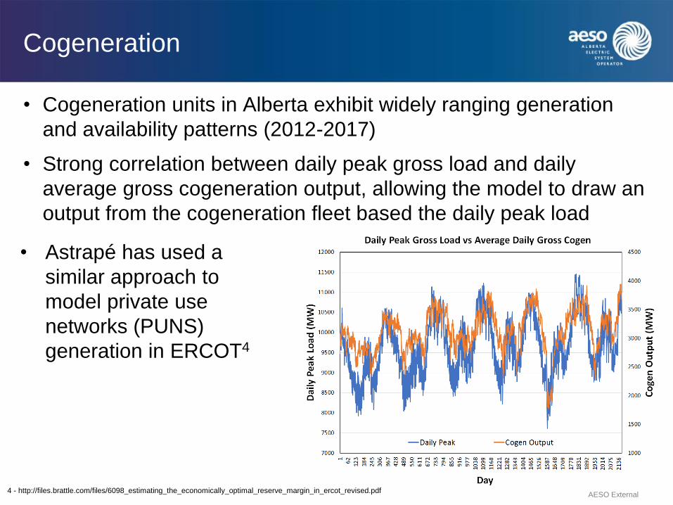
• Cogeneration units in Alberta exhibit widely ranging generation
and availability patterns (2012-2017)
• Strong correlation between daily peak gross load and daily
average gross cogeneration output, allowing the model to draw an
output from the cogeneration fleet based the daily peak load
AESO External
• Astrapé has used a
similar approach to
model private use
networks (PUNS)
generation in ERCOT4
4 - http://files.brattle.com/files/6098_estimating_the_economically_optimal_reserve_margin_in_ercot_revised.pdf

Cogeneration
• Aggregation was performed by adding the historical
availability capacity (AC) from generators then normalized by
the installed capacity at each hour
• The daily peak load and daily peak available capacity were
calculated for the aggregate. This was grouped into a
number of normalized load levels each with a distribution of
the cogeneration availability
• The model then randomly draws cogeneration multipliers for
each day
AESO External

Cogeneration
• An example, when
daily peak load is
85-89% of annual
peak load, the
model will draw a
multiplier of 61% to
84% (the green line)
• The drawn value is
multiplied by the
installed capacity of
approximately 5,000
MW to determine
the daily generation
of the cogeneration
fleet
AESO External

Emergency Response/Ancillary Services
• Emergency operations modeling plays a significant role in evaluating loss of load
events
– BAL-002-WECC-AB1-25 and System Controller Procedures6 outline our current
guidelines
• AESO will model EEA1 and EEA2 hours by measuring how often RAM
dispatches contingency reserves
– Supplemental Reserves (Quick Start)
– Spinning Reserves (Spinning Reserves)
• Firm Load shed will begin once contingency reserves are depleted, but regulating
reserves will be maintained even during load shed events
– Reserves are calculated as a percentage of load and then allocated to an eligible
resource units capacity and then only activated once all remaining in-merit energy is
dispatched, representing an EEA event
• Spinning Reserves (2.5% of Gross Load)
• Supplemental Reserves (2.5% of Gross Load)
• Regulating Reserve (1.5% of Gross Load)
AESO External
5 - https://www.aeso.ca/assets/documents/BAL-002-WECC-AB1-2.pdf
6 - http://ets.aeso.ca/ets_web/ip/Market/Reports/HelpTextServlet?service=EnergyAlertsInfo

Reserve Margin
• NERC defines RM as Percentage of additional capacity over load
– Reserve Margin (%) = (Capacity – Load)/Load X 100
– Generally measured over Peak Load
• Other regions generally include nameplate capacity for thermal resources
and derated intermittent resource values according to expected resource
adequacy benefit.
• RAM results are displayed with an ICAP figure then a capacity credit is
applied to calculate a reserve margin to evaluate results
AESO External

Generation Additions - Reference Unit
• For resource adequacy modeling a reference unit is selected
to allow the model to evaluate different reserve margin levels
• Resource adequacy intention is to align with the reference
technology selected to calculate cost of new entry
• Current assumed generic expansion unit characteristics
– Nameplate Capacity – 47.5 MW
– Fuel/Technology – SC gas
– Forced Outage Rate of 3%
AESO External
Draft – Results
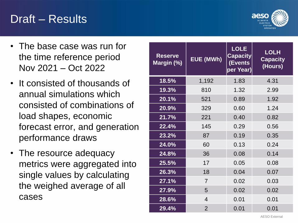
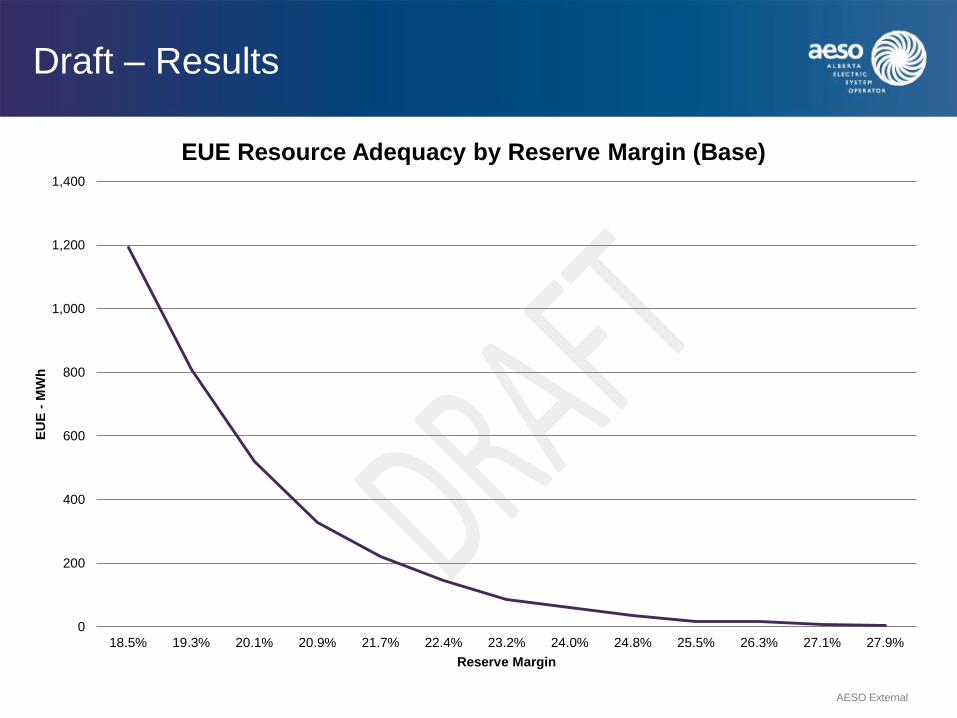
• The base case was run for
the time reference period
Nov 2021 – Oct 2022
• It consisted of thousands of
annual simulations which
consisted of combinations of
load shapes, economic
forecast error, and generation
performance draws
• The resource adequacy
metrics were aggregated into
single values by calculating
the weighed average of all
cases
Reserve
Margin (%) EUE (MWh)
LOLE
Capacity
(Events
per Year)
LOLH
Capacity
(Hours)
18.5% 1,192 1.83 4.31
19.3% 810 1.32 2.99
20.1% 521 0.89 1.92
20.9% 329 0.60 1.24
21.7% 221 0.40 0.82
22.4% 145 0.29 0.56
23.2% 87 0.19 0.35
24.0% 60 0.13 0.24
24.8% 36 0.08 0.14
25.5% 17 0.05 0.08
26.3% 18 0.04 0.07
27.1% 7 0.02 0.03
27.9% 5 0.02 0.02
28.6% 4 0.01 0.01
29.4% 2 0.01 0.01
AESO External
Draft – Results
AESO External
0
200
400
600
800
1,000
1,200
1,400
18.5% 19.3% 20.1% 20.9% 21.7% 22.4% 23.2% 24.0% 24.8% 25.5% 26.3% 27.1% 27.9%
EU
E -
MW
h
Reserve Margin
EUE Resource Adequacy by Reserve Margin (Base)
Draft – Results
AESO External
0
5
10
15
20
25
30
18.5% 19.3% 20.1% 20.9% 21.7% 22.4% 23.2% 24.0% 24.8% 25.5% 26.3% 27.1% 27.9%
An
nu
al
Ho
ur
Co
un
t
Reserve Margin
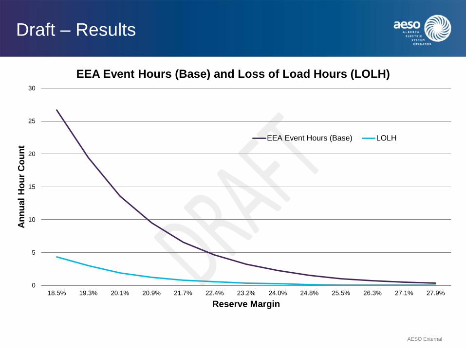
EEA Event Hours (Base) and Loss of Load Hours (LOLH)
EEA Event Hours (Base) LOLH

Draft – Results Monthly
AESO External
0
20
40
60
80
100
120
140
160
Jan Feb Mar Apr May Jun Jul Aug Sep Oct Nov Dec
EU
E (
MW
h)
Monthly EUE Values for different Reserve Margins
20.10% 20.90% 21.70% 22.40% 23.20%

Draft – Results Monthly
• Resource adequacy problems are more distributed
throughout the year for AESO than for utilities with a higher
degree of seasonality and more load responsiveness to
weather conditions.
AESO External
• Given the high AESO
load factor and
transmission availability
risk, the level of
reserves is required
may be higher than
other systems across
the industry.

Next Steps
• Seek and respond to feedback on:
– Set of inputs currently in the model
– Methodology used to calculate inputs and results
– Additional inputs or uncertainties AESO should consider
• AESO will continue to validate model and perform additional
sensitivities to assist with calibration
• Continue to align with other streams of the capacity market
design (UCAP, Demand Curve, etc)
AESO External

Additional Material for Information
AESO External
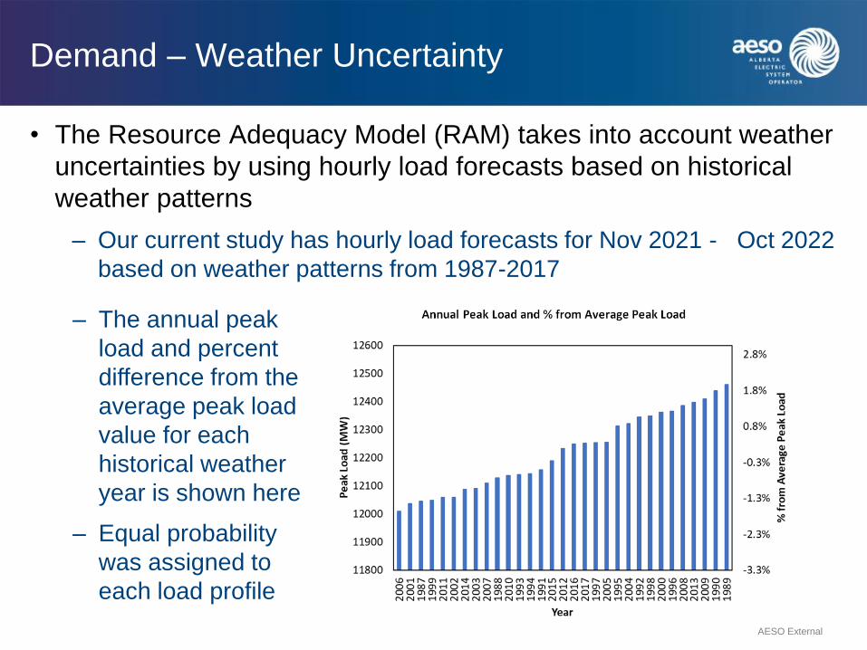
Demand – Weather Uncertainty
• The Resource Adequacy Model (RAM) takes into account weather
uncertainties by using hourly load forecasts based on historical
weather patterns
– Our current study has hourly load forecasts for Nov 2021 - Oct 2022
based on weather patterns from 1987-2017
– The annual peak
load and percent
difference from the
average peak load
value for each
historical weather
year is shown here
– Equal probability
was assigned to
each load profile
AESO External
Demand – Economic Uncertainty
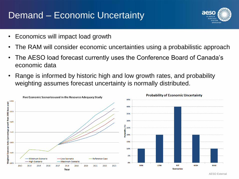
• Economics will impact load growth
• The RAM will consider economic uncertainties using a probabilistic approach
• The AESO load forecast currently uses the Conference Board of Canada’s
economic data
• Range is informed by historic high and low growth rates, and probability
weighting assumes forecast uncertainty is normally distributed.
AESO External

Intertie
• Interties are modeled as pseudo units
because the transmission capability
was identified as the binding market
support constraint rather than the
generation availability from
neighboring markets
• Historical ATC data was analyzed and
a tie-line availability distribution was
created subject to transfer constraints
• The model draws the same percentile
for each intertie to allow for high and
low availability to occur in all regions
simultaneously
• Due to the nature of this modelling
being focused on the physical resource
adequacy assessment, imports were
set to occur after the dispatch of
AESO’s last resource
AESO External
Percentile
of Capacity
Limit In (%)
BCHA ->
AESO (MW)
MT ->
AESO
(MW)
SASK ->
AESO (MW)
0 0 0 0
10 635.0 0 0
20 750.0 0 0
30 750.0 47.8 0
40 750.0 90.1 0
50 750.0 174.0 0
60 750.0 182.0 30.4
70 750.0 190.6 41.0
80 750.0 200.7 68.0
90 750.0 210.0 100.0
100 780.0 225.0 152.5

Renewable – Wind
• Simulated wind shapes were developed using historical metered
output from existing sites from 2005-2017
– The data was initially normalized by dividing each hourly output by
the maximum output of the site
– The shapes were then aggregated by geographic locations according
to wind output correlations
AESO External
– Aggregated profiles were
assigned to each existing and
future wind farms
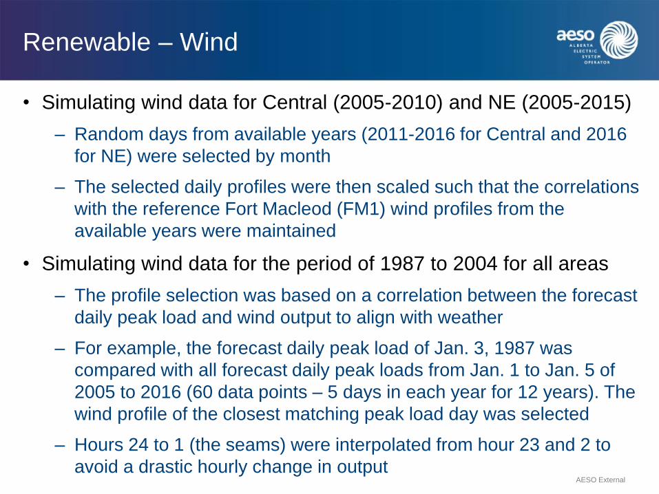
Renewable – Wind
• Simulating wind data for Central (2005-2010) and NE (2005-2015)
– Random days from available years (2011-2016 for Central and 2016
for NE) were selected by month
– The selected daily profiles were then scaled such that the correlations
with the reference Fort Macleod (FM1) wind profiles from the
available years were maintained
• Simulating wind data for the period of 1987 to 2004 for all areas
– The profile selection was based on a correlation between the forecast
daily peak load and wind output to align with weather
– For example, the forecast daily peak load of Jan. 3, 1987 was
compared with all forecast daily peak loads from Jan. 1 to Jan. 5 of
2005 to 2016 (60 data points – 5 days in each year for 12 years). The
wind profile of the closest matching peak load day was selected
– Hours 24 to 1 (the seams) were interpolated from hour 23 and 2 to
avoid a drastic hourly change in output AESO External

Renewable – Wind
AESO External

Renewable – Solar
• Simulated solar shapes were developed
using the NREL National Solar Radiation
Database (NSRDB) Data Viewer and
System Advisory Model (SAM) to generate
the hourly solar profiles for 1998 to 2016
• Solar profiles for 1987 to 1997 and 2017
used the same daily peak load look-up
technique as creating wind profiles for
1987 to 2004
• Ten profiles were created using the inputs
and assigned to our existing asset and
would be assigned to future assets.
– 5 geographic locations
– 2 technology (fixed & tracking solar PV)
August Fixed Solar Profiles
August Tracking Solar Profiles
AESO External

Renewable – Hydro
• Actual hourly hydro data was
analyzed from 2012 to 2017 and an
aggregated profile was created
• The minimum and maximum daily
dispatch levels and monthly maximum
dispatch levels can be defined as a
function of the total monthly hydro
energy
• Curve fit equations applied to
historical monthly energy 2001-2017
• For years without monthly energy
availability (1987-2001), data from the
year that most closely matched
average annual snowfall (2001-2017)
was used
AESO External

Renewable – Hydro
• RAM optimally schedules the hourly
hydro energy based on each day’s
hourly load shape while respecting
daily and monthly dispatch constraints
• The following values are identified and
used to constrain the dispatch logic
– Average daily minimum
– Maximum dispatch levels
– Total monthly energy
– Monthly maximum dispatch levels
• After minimum weekly flows are taken
into account, the remainder of the
month’s energy is scheduled as peak
shaving respecting the totally monthly
hydro constraint
AESO External
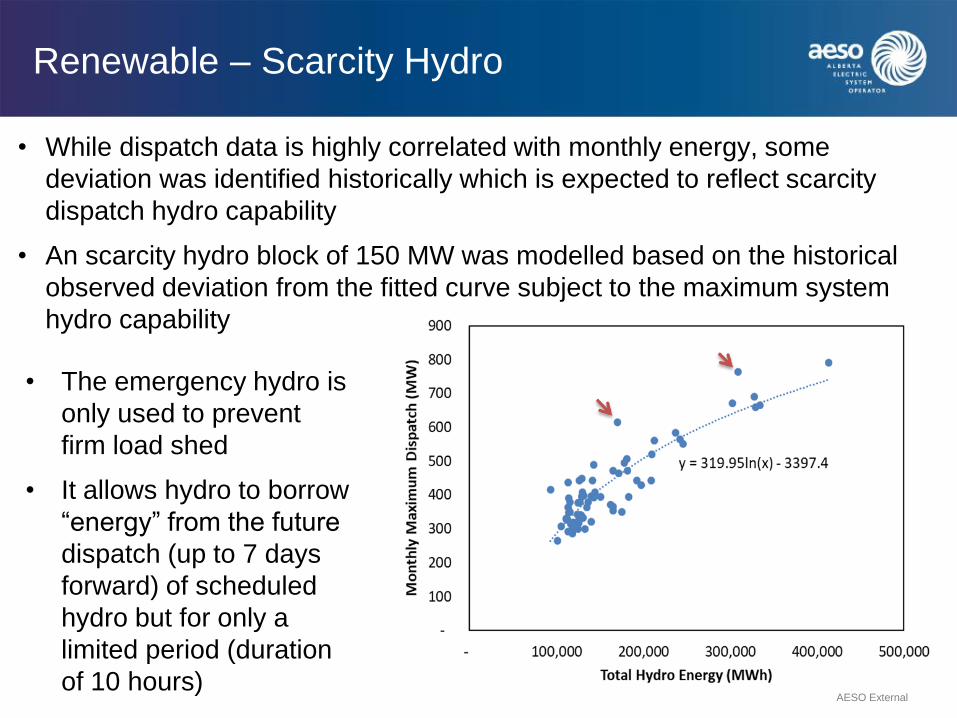
Renewable – Scarcity Hydro
• While dispatch data is highly correlated with monthly energy, some
deviation was identified historically which is expected to reflect scarcity
dispatch hydro capability
• An scarcity hydro block of 150 MW was modelled based on the historical
observed deviation from the fitted curve subject to the maximum system
hydro capability
AESO External
• The emergency hydro is
only used to prevent
firm load shed
• It allows hydro to borrow
“energy” from the future
dispatch (up to 7 days
forward) of scheduled
hydro but for only a
limited period (duration
of 10 hours)
Appendix
AESO External
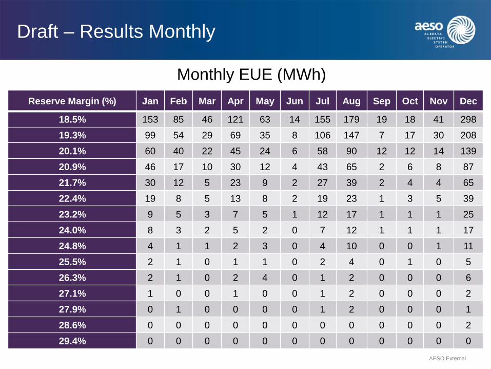
Draft – Results Monthly
Reserve Margin (%) Jan Feb Mar Apr May Jun Jul Aug Sep Oct Nov Dec
18.5% 153 85 46 121 63 14 155 179 19 18 41 298
19.3% 99 54 29 69 35 8 106 147 7 17 30 208
20.1% 60 40 22 45 24 6 58 90 12 12 14 139
20.9% 46 17 10 30 12 4 43 65 2 6 8 87
21.7% 30 12 5 23 9 2 27 39 2 4 4 65
22.4% 19 8 5 13 8 2 19 23 1 3 5 39
23.2% 9 5 3 7 5 1 12 17 1 1 1 25
24.0% 8 3 2 5 2 0 7 12 1 1 1 17
24.8% 4 1 1 2 3 0 4 10 0 0 1 11
25.5% 2 1 0 1 1 0 2 4 0 1 0 5
26.3% 2 1 0 2 4 0 1 2 0 0 0 6
27.1% 1 0 0 1 0 0 1 2 0 0 0 2
27.9% 0 1 0 0 0 0 1 2 0 0 0 1
28.6% 0 0 0 0 0 0 0 0 0 0 0 2
29.4% 0 0 0 0 0 0 0 0 0 0 0 0
AESO External
Monthly EUE (MWh)

UCAP Calculation Methodology
Technical Workgroup #2
April 6th, 2018
72
Agenda
• Summarizing Feedback from TWG #1
• More details on how assets are classified between Availability Factor (AF) & Capacity
Factor(CF)
• Used Metered Volumes vs Dispatch Levels to assess whether assets were true to their dispatch levels
• Further information on calculation considerations
• Denominators for Capacity Factor
• Inclusion of ancillary services
• Weighted average Availability Capability for use in Availability Factors
• Calculation approach for assets that have mothballed
• Supply cushion Analysis
– Selection of Supply cushion (mid hour, top hour, weighted)
– Applying supply cushion size constraint to 100 tightest hours
• Asset Specific Information – Impacts to UCAP (Appendix)

Feedback on proposed UCAP calculation
• Generally, half the members agreed on using 100 hours and 5 years historical data. The
other half were conditional yes’s, neutral or no’s. Additional asks from the conditional yes’s
were:
– Ensure alignment to resource adequacy
– Asset specific information to determine variation in UCAP
– Removal of planned outages
– Analysis of MW and supply cushion thresholds, resulting in less than 100 hours for some years
• For those that were not supportive suggested:
– Future not reflective of past
– Use more hours instead of 100
– Alignment to resource adequacy
– AESO does not have enough data
– Asset specific analysis required before decision
The AESO will be continuing with the proposed AF & CF approach, work for future CMDs will
be focused on defining and refining details of the AF & CF approach
73

Classification of assets between AF & CF
approach
74
Availability factor
= Weighted
Available Capability/
Maximum Capability
Capacity factor =
Metered Volumes /
Maximum Capability
N Y
Are dispatches
reflective of metered
volumes?
UCAP = Performance factor time
MC (Current or Future)

Classification of assets
75
Availability factor
= Weighted
Available Capability/
Maximum Capability
Capacity factor =
Metered Volumes/
Maximum Capability
N Y
All coal and hydro,
Most combined cycle, Most
Simple Cycle,
[Cogen] BCR2, BCRK, CNR5,
FH1, JOF1, MEG1, PW01, RL1,
SCL1, TC01, TLM2, UOA1,
MKRC
Most ‘Other’
[CC] MEDHAT ,FNG1,
[SC] ANC1,
[Cogen] SHELL, DOWG, EC04, IMPOIL,
MKR1, NX02, PR1, SUNCOR, TC02,
HMT1, CL01, UOC1
[Other] GPEC, WEY1
All Wind
Are dispatches
reflective of metered
volumes?
UCAP = Performance factor times
MC (Current or Future)
Exception: There are five assets that don’t meet either criteria, AESO continues to work through these

Further information on calculation
considerations
AESO will be using:
1) Maximum Capability of individual assets for the denominator of capacity
factor calculation, instead of maximum metered volumes. Metered volumes
are prone to significant variation and not a reasonable reflection of assets
capability
2) For Inclusion of ancillary services volumes for capacity factor resources,
AESO will be using Metered Volumes plus dispatched and/or directives
3) Weighted average Available Capability over the hour will be used to
represent the assets availability as this is an accurate representation of the
availability of an asset
76

Accounting for Mothballing of asset in UCAP
calculation
Available Capability during a mothball outage is not indicative of a
generators ability to produce capacity.
• Mothball methodology
– Exclude the tight supply cushion hours when the asset is mothballed
– Take the simple average over all of the remaining hours (e.g. If an asset had 82
mothballed hours in 2016/17, the average would be taken over 412 hours)
– If below a statistically significant value, use a combination of existing data to establish
a UCAP.
Other options considered, but discarded:
1. Replace mothballed time with group average
• Discarded because distort assets actual performance
77
Year 1 Year 2 Year 3 Year 4 Year 5
Hours 100 100 100 100 12 82 Normal Op Normal Op Normal Op Normal Op Normal Op
Normal Op
Mothball

Supply Cushion Analysis
• Selection of hourly supply cushion value
– Mid hour – Snapshot at 30th minute of hour
– End of hour – Snapshot at 59th minute of the hour
– Weighted average – duration weighted average within the hour
• Use of additional constraints
– Compared 100 hours base case to a frontier scenario
78

Selection of Supply Cushion hours
• Duration-weighted average is gold standard calculation methodology
• Requires high-quality data
• Implementation requires IT resources
• Representative of true supply cushion
• Mid-hour snapshot could proxy duration-weighted average
• Over 90% common observations
• Already in production
• Can act as a reasonable proxy to duration weighted average calculation
AESO will be using the duration weighted average going forward
380
15 81
24
17
26
79
59th minute
snapshot 30th minute
snapshot
Duration weighted
average
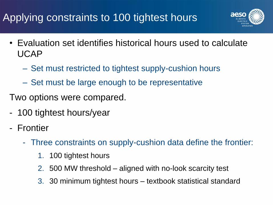
Applying constraints to 100 tightest hours
• Evaluation set identifies historical hours used to calculate
UCAP
– Set must restricted to tightest supply-cushion hours
– Set must be large enough to be representative
Two options were compared.
- 100 tightest hours/year
- Frontier
- Three constraints on supply-cushion data define the frontier:
1. 100 tightest hours
2. 500 MW threshold – aligned with no-look scarcity test
3. 30 minimum tightest hours – textbook statistical standard
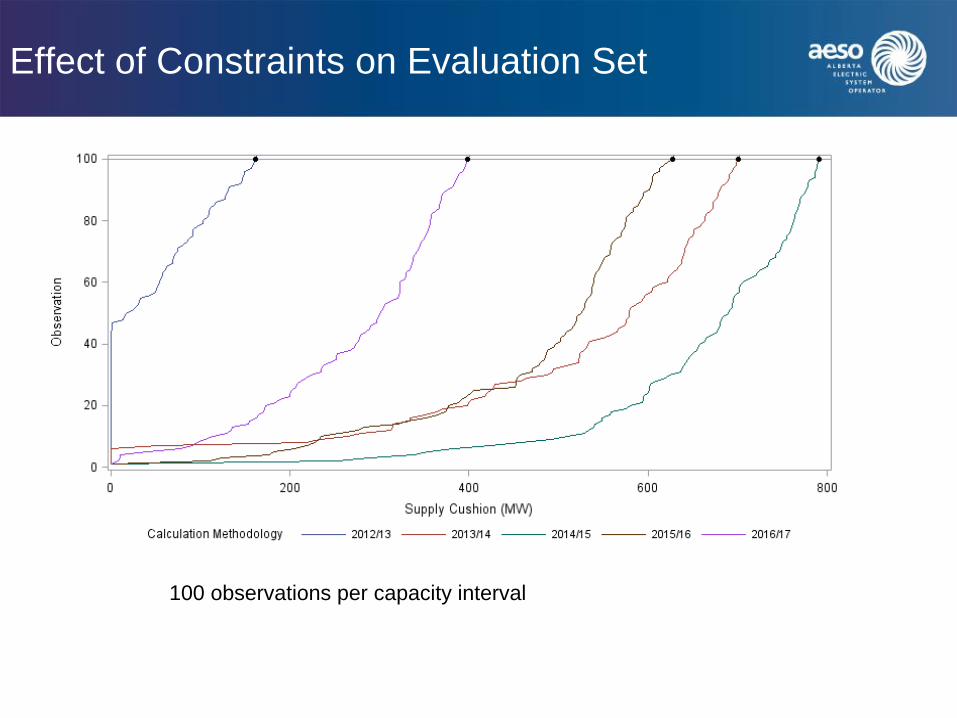
Effect of Constraints on Evaluation Set
100 observations per capacity interval

Selecting the Evaluation Set
• Options
– Leave at 100 tightest hours per year
– Impose 500 MW supply cushion threshold and also minimum sample n>= 30
per year
82
100 hours 500 MW and at least 30
tightest hours
Advantage Simpler to implement and explain Targets specific hours where reliability
is a concern. Will eliminate hours in
which there was adequate supply
Disadvantage May include hours where supply
cushion is considered “healthy”
Smaller sample size in high supply
cushion years
Potential that the number of hours
used changes year-to-year
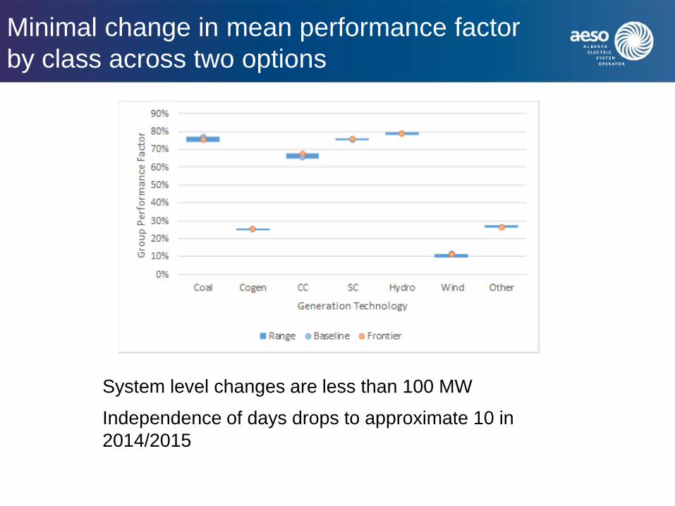
Minimal change in mean performance factor
by class across two options
System level changes are less than 100 MW
Independence of days drops to approximate 10 in
2014/2015
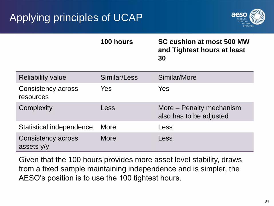
Applying principles of UCAP
100 hours SC cushion at most 500 MW
and Tightest hours at least
30
Reliability value Similar/Less Similar/More
Consistency across
resources
Yes Yes
Complexity Less More – Penalty mechanism
also has to be adjusted
Statistical independence More Less
Consistency across
assets y/y
More Less
84
Given that the 100 hours provides more asset level stability, draws
from a fixed sample maintaining independence and is simpler, the
AESO’s position is to use the 100 tightest hours.

Appendix

Preliminary Asset Specific Statistics - Coal
86
0.0%
10.0%
20.0%
30.0%
40.0%
50.0%
60.0%
70.0%
80.0%
90.0%
100.0%
GN3 SH1 GN2 BR4 SH2 BR5 BR3 GN1 SD3 KH3 SD4 SD6 KH2 SD5 KH1 HRM SD2 SD1
Perf
orm
an
ce F
acto
r
Base Case (100 observations per capacity interval) Frontier (500 MW max; 30 to 100 observations per capacity interval)
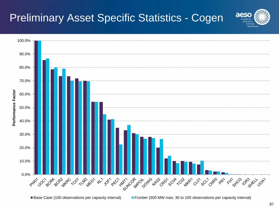
Preliminary Asset Specific Statistics - Cogen
87
0.0%
10.0%
20.0%
30.0%
40.0%
50.0%
60.0%
70.0%
80.0%
90.0%
100.0%
Perf
orm
an
ce F
acto
r
Base Case (100 observations per capacity interval) Frontier (500 MW max; 30 to 100 observations per capacity interval)
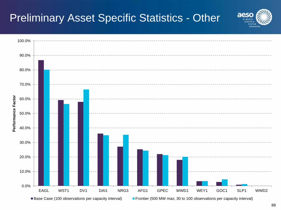
Preliminary Asset Specific Statistics - Other
88
0.0%
10.0%
20.0%
30.0%
40.0%
50.0%
60.0%
70.0%
80.0%
90.0%
100.0%
EAGL WST1 DV1 DAI1 NRG3 AFG1 GPEC WWD1 WEY1 GOC1 SLP1 WWD2
Perf
orm
an
ce F
acto
r
Base Case (100 observations per capacity interval) Frontier (500 MW max; 30 to 100 observations per capacity interval)

Preliminary Asset Specific Statistics - SC
89
0.0%
10.0%
20.0%
30.0%
40.0%
50.0%
60.0%
70.0%
80.0%
90.0%
100.0%
Perf
orm
an
ce F
acto
r
Base Case (100 observations per capacity interval) Frontier (500 MW max; 30 to 100 observations per capacity interval)

Preliminary Asset Specific Statistics - Wind
90
0%
5%
10%
15%
20%
25%
Perf
orm
an
ce F
acto
r
Base Case (100 observations per capacity interval) Frontier (500 MW max; 30 to 100 observations per capacity interval)

Preliminary Asset Specific Statistics - CC
91
0.0%
10.0%
20.0%
30.0%
40.0%
50.0%
60.0%
70.0%
80.0%
90.0%
100.0%
EC01 NX01 CAL1 EGC1 FNG1 MEDHAT
Perf
orm
an
ce F
acto
r
Base Case (100 observations per capacity interval) Frontier (500 MW max; 30 to 100 observations per capacity interval)