temperature and the allocation of time: implications … and the allocation of time: implications...
TRANSCRIPT
NBER WORKING PAPER SERIES
TEMPERATURE AND THE ALLOCATION OF TIME:IMPLICATIONS FOR CLIMATE CHANGE
Joshua Graff ZivinMatthew J. Neidell
Working Paper 15717http://www.nber.org/papers/w15717
NATIONAL BUREAU OF ECONOMIC RESEARCH1050 Massachusetts Avenue
Cambridge, MA 02138February 2010
We thank Eli Berman, Janet Currie, Partha Deb, Sherry Glied, Gordon Hanson, Ryan Kellogg, WojtekKopczuk, Robert Mendelsohn, Michael Roberts, Hilary Sigman, Till von Wachter, and Ty Wilde andseminar participants at Yale University, the University of Illinois - Chicago, the University of Maryland,the Northeastern Conference in Environmental and Natural Resource Economics, and the TriangleResource and Environmental Economics Seminar Series for numerous useful comments. We alsothank Ashwin Prabhu for excellent research assistance. We are particularly indebted to Wolfram Schlenkerfor many helpful discussions and for generously sharing data. The views expressed herein are thoseof the authors and do not necessarily reflect the views of the National Bureau of Economic Research.
NBER working papers are circulated for discussion and comment purposes. They have not been peer-reviewed or been subject to the review by the NBER Board of Directors that accompanies officialNBER publications.
© 2010 by Joshua Graff Zivin and Matthew J. Neidell. All rights reserved. Short sections of text, notto exceed two paragraphs, may be quoted without explicit permission provided that full credit, including© notice, is given to the source.
Temperature and the Allocation of Time: Implications for Climate ChangeJoshua Graff Zivin and Matthew J. NeidellNBER Working Paper No. 15717February 2010JEL No. J22,Q54
ABSTRACT
In this paper we estimate the impacts of climate change on the allocation of time using econometricmodels that exploit plausibly exogenous variation in daily temperature over time within counties. We find large reductions in U.S. labor supply in industries with high exposure to climate and similarlylarge decreases in time allocated to outdoor leisure. We also find suggestive evidence of short-runadaptation through temporal substitutions and acclimatization. Given the industrial compositionof the US, the net impacts on total employment are likely to be small, but significant changes in leisuretime as well as large scale redistributions of income may be consequential. In developing countries,where the industrial base is more typically concentrated in climate-exposed industries and baselinetemperatures are already warmer, employment impacts may be considerably larger.
Joshua Graff ZivinInternational Relations & Pacific StudiesUniversity of California, San Diego9500 Gilman Drive, MC 0519La Jolla, CA 92093-0519and [email protected]
Matthew J. NeidellDepartment of Health Policy and ManagementColumbia University600 W 168th Street, 6th FloorNew York, NY 10032and [email protected]

1. Introduction
Climate change is expected to warm the earth considerably in the coming decades. These
temperature changes, in turn, are likely to exert profound impacts on the way in which humans
interact with the planet. One important aspect of life that is likely to be transformed under a new
climatic paradigm is individual decisions regarding the allocation of their time. Higher
temperatures can lead to changes in time allocated to work by altering the marginal productivity
of labor (or the marginal cost of supplying labor), especially in climate-exposed industries, such
as agriculture, construction, and manufacturing.2 Higher temperatures may also change the
marginal utility of leisure activities,3 altering the distribution of time allocated to non-work
activities. Each of these responses will, in turn, generate indirect impacts through tradeoffs
between labor and leisure. Since time is a limited but extremely valuable resource, the welfare
implications associated with these climate-induced reallocations of time are potentially quite
large.4
In this paper we estimate the impacts of climate on the allocation of time to labor as well
as leisure activities. Our paper is unique in at least two regards. First, it is the only analysis, to
our knowledge, of the impacts of climate on labor supply5 – the primary source of household
income throughout the world. Our understanding of this relationship is also important because it
sheds light on the micro-foundations for the macroeconomic literature that has focused on
2The marginal productivity of labor may be influenced through impacts on endurance, fatigue, and cognitive performance. See Gonzalez-Alonso et al., 1999; Galloway and Maughan, 1997; Nielsen et al. 1993 for evidence on endurance and fatigue. See Epstein et al. (1980), Ramsey (1995), Hancock et al. (2007), Pilcher et al. 2002 for evidence on cognitive performance. 3 See Ma et al., 2006; Pivarnik et al., 2003; U.S. Department of Health and Human Services, 1996; Eisenberg and Okeke, 2008 for evidence on the relationship between temperature and various leisure activities. 4 Although our paper is concerned with welfare impacts from climate change, the partial equilibrium nature of our analysis precludes us from making welfare calculations. For a more general analysis of welfare impacts at the household level, see Albouy et al. (2009). 5 Note that while we use the terminology labor supply throughout the paper, we are referring to equilibrium employment levels due to perturbations in supply and demand.
2

climate and economic growth (Sachs and Warner, 1996; Nordhaus, 2006, Dell et al., 2008). It
also provides a direct test of the exogenous labor supply assumption embedded in most of the
Integrated Assessment Models that are used to simulate the economic impacts of climate change
and that play a prominent role in the design of climate change policies.
Second, individuals’ allocation of time in response to temperature represents an avenue
for exploring potential adaptations that may minimize welfare effects from climate change.6
Activity choice and location should be viewed as a form of avoidance behavior whereby
individuals protect themselves from the heat by, perhaps, spending more time indoors on hot
days. We further probe short- to medium-run adaptation strategies through an examination of
intra- and inter-temporal reallocations of time as well as through acclimatization, whereby
weather tolerance is altered by prior climate experience such that, for example, Minnesotans may
act more like Floridians once their climate warms. While new climate-neutralizing technologies
will almost certainly be invented in the coming century, these estimates deepen our
understanding about what is possible given the existing technology set and, in turn, the potential
value of innovations that help us to cope with climate change in the future.
We begin our analysis by estimating the impacts of temperature on time allocation using
individual level data from the 2003-2006 American Time Use Surveys (ATUS) linked to daily
weather data from the National Climatic Data Center. Our econometric models include year-
month and county fixed effects, which enables us to identify the effects of temperature using the
plausibly exogenous variation in temperature over time within counties and within seasons.7 We
flexibly model temperature by including a series of indicator variables for five degree
6 Our work could also be viewed as a general equilibrium extension of the numerous studies that have focused on the impacts of climate change on circumscribed sets of leisure activities (see, for example, Loomis and Crespi, 1999; Mendelsohn and Markowski, 1999; Englin and Moeltner, 2004). 7 This identification strategy has also been employed in other studies examining various aspects of climate change (Schlenker et al., 2005; Deschenes and Greenstone 2007a and 2007b).
3

temperature bins, with the highest bin for days over 100 degrees. One of the tremendous
advantages of using the ATUS is that we can exploit data from the 2006 heat wave that produced
high temperatures across much of the United States to produce more reliable estimates of
behavioral responses at the high end of the temperature distribution.8
In exploring the scope for adaptation, we focus our attention on the high end of the
temperature distribution since our interest in this question is driven by concerns about climate
change under which the low end of the distribution will get warmer and thus easier to manage.
We examine potential short-run compensatory behavior by testing to see whether individuals re-
allocate activities across days by comparing the impacts of lagged temperature to that of
contemporaneous temperature. We complement this analysis with an examination of
intratemporal substitution, i.e. moving climate-exposed activities from daylight to twilight hours.
The role of acclimatization in adaptive strategies is investigated over both the short and medium-
run. The former relies on comparisons of responses at different points in the summer season,
with the notion that hot days may be easier to tolerate in August than in June when they have just
begun to arrive. To analyze the latter, we stratify our model by historical climate to obtain
separate short-run responses for traditionally hotter vs. colder places. It is important to note that,
in general, our tests for adaptation are underpowered. As a result we view this work as
exploratory, but perhaps the best that can be done given pressing concerns about societal
responses to climate change and the limited data availability under current climatic conditions.
Our results reveal impacts on a wide range of activities. While we find suggestive
evidence of a moderate decline in aggregate labor supply response at high temperatures, further
analysis reveals considerable heterogeneity across industry sectors based on their exposure to
8 The 2006 heat wave covered most of the U.S. from mid-July through early-August. For example, beginning on July 17, every state except Alaska experienced a high temperature over 90 degrees for three consecutive days based on our weather data (described below).
4

climatic elements. At temperatures above 85 degrees Fahrenheit, workers in industries with high
exposure to climate reduce daily labor supply by as much as one hour. Almost all of the
decrease in labor supply happens at the end of the day when fatigue from prolonged exposure to
heat has likely set in. We find limited evidence consistent with adaptation to higher
temperatures, recognizing demand factors may limit workers discretion in choosing labor supply.
In terms of leisure activities, we generally find an inverted U-shaped relationship with
temperature for outdoor leisure and a corresponding U-shaped relationship for indoor leisure.
This relationship is most pronounced for those not currently employed, as they have the most
flexibility in their scheduling. Overall, these results suggest that protective behavior in response
to warmer temperatures may provide an important channel for minimizing the impacts of heat.
Temporal substitutions as well as acclimatization also appear to mute the impacts of extreme
heat, although these findings are often not significant at conventional levels, in part, because of
limited sample size when the data are disaggregated at the high end of the distribution.
The impacts on labor supply are non-trivial. If temperatures were to rise by 5 degrees
Celsius in the U.S. by the end of the coming century9 and no adaptation occurs, U.S. labor
supply would fall by roughly 0.6 hours per week in high-exposure industries, representing a
1.7% decrease in hours worked and thus earnings. In developing countries, where industrial
composition is generally skewed toward climate-exposed industries and prevailing temperatures
are already hotter than those in most of the US, the economic impacts are likely to be much
larger.
The remainder of our paper is organized as follows. The next section provides a
conceptual framework for the analysis of climate change impacts on time allocation decisions.
9 This temperature increase loosely corresponds with the business-as-usual emissions scenario (A2) forecast from the Intergovernmental Panel on Climate Change Fourth Assessment Report (http://www.ipcc.ch/).
5

Section 3 describes the data and Section 4 details our econometric approach. The results are
presented in Section 5. Section 6 concludes.
2. Conceptual Framework
High temperatures cause discomfort, fatigue, and even cognitive impairment depending
on the composition of one’s activities and the degree to which they are exposed to the elements.
For simplicity, we imagine that individuals allocate their total time in a day across three broad
activity categories: work, outdoor leisure, and indoor leisure.10 Since one of our outcomes of
interest is the impact of temperature on labor supply, we distinguish between two types of
workers based on exposure to climate – those that are generally sheltered from climate and those
that are not. We refer to the former as having low risk of exposure to climate (‘low-risk’) and
the latter as having high risk of exposure to climate (‘high-risk’). We also separately focus on
those not employed where they only allocate their time to outdoor and indoor leisure activities.
We begin with a description of the labor-leisure tradeoff for those in the high-risk sector.
As summer temperatures increase for these individuals, the marginal utility from outdoor leisure
falls, the marginal productivity of their labor falls, and, given the near-omnipresence of air
conditioning in the US11, the marginal utility from indoor leisure is mostly unchanged. As a
result, time is re-allocated from work and outdoor leisure to indoor leisure activities.12 In
10 In our original specification we also included sleep because it may be affected through changes in the marginal utility of labor or leisure (Biddle and Hamermesh, 1990), but since it proved insensitive to temperature we focus on the allocation of time over waking hours. 11 According to the 2001 American Housing Survey, 79.5% of all household had some form of air conditioning, with the rate of ownership much higher in warmer regions. 12 Technically, high temperatures could also lead to an increase in work (outdoor leisure) if the marginal utility of the last hour of indoor leisure were smaller than the utility gain from the consumption associated with the first additional hour of work (the first additional hour of outdoor leisure). For this to obtain, the marginal utility of indoor leisure would have to be decreasing at a sharply increasing rate while the other functions remain relatively flat.
6
contrast, increasing winter temperatures lead to reallocations away from indoor leisure and into
work and outdoor activities. These seasonal effects need not be symmetric.
The tradeoff is slightly different for those in the low-risk sector since hotter summers
only directly affect the marginal utility they receive from outdoor activities. In this case, time is
re-allocated from outdoor leisure to indoor leisure and work. The division between these
climate-sheltered activities depends on the relative returns to allocating additional hours to
each.13 As with the high-risk case, the effects in winter work in the opposite direction,
potentially yielding reductions in work and indoor leisure time.
For those individuals that are not employed, the tradeoff is much more straightforward.
Increased heat in the summer leads to more leisure time spent indoors, while increased heat in
other seasons will lead to more leisure time spent outside. Since leisure decisions for this group
do not depend on equilibrium outcomes in the labor market, we expect these individuals to be
more responsive to changes in temperatures than those who are employed.
The models described above allow for little adaptation to changes in climate, and hence
best describe a partial picture of short run behavioral responses to temperature.14 On hot days,
individuals may shift activities to cooler moments within the day (intratemporal substitution) or
simply postpone them until cooler days arrive (intertemporal substitution). In addition to
adaptation through behavioral changes, individuals may acclimatize (or habituate) to new
temperatures.15 Physiological acclimatization arises through numerous channels, including
changes in skin blood flow, metabolic rate, oxygen consumption, and core temperatures
13 More formally, the tradeoff will depend on the relative slopes of the marginal utility curve for indoor leisure and the marginal productivity of labor at the old climate equilibrium, i.e. it depends on the second derivatives of the utility and production functions with respect to hours. 14 While adaptation typically refers to long run changes, we view any action that minimizes the potential welfare impacts from climate change as adaptation. 15 In the behavioral economics literature this is referred to as reference dependent preferences (see Rabin, 1998)
7

(Armstrong and Maresh, 1991). It can occur in short periods of time – up to two weeks in
healthy individuals under controlled training regimens – but longer for unhealthy individuals or
those experiencing passive exposure (Wagner et al., 1972). Over longer periods of time,
behavioral acclimatization may also enable individuals to adjust to changes in climate through
the adoption of various technologies to cope with unpleasant temperatures.16 These forms of
short- and medium-term adaptation, which are essential for understanding potential individual
level adaptations to climate change, are probed further in the analysis that follows.
3. Data
3.A. ATUS
The American Time Use Survey (ATUS) is a nationally representative survey available
from 2003-06 describing how and where Americans spend their time. Respondents are
individuals over age 15 randomly selected from households that have completed their final
month in the Current Population Survey (CPS). Each respondent completes a 24-hour time diary
for a pre-assigned date, providing details of the activity undertaken, the length engaged in the
activity, and where the activity took place. Each respondent is interviewed the day after the
diary date, and is contacted for 8 consecutive weeks to obtain an interview.
We classify individuals into three groups. For the first two groups, we separate workers
into high and low risk of exposure to climate based on National Institute of Occupational Safety
(NIOSH) definitions of heat-exposed industries (NIOSH, 1986) and industry codes in the ATUS.
These include industries where the work is primarily performed outdoors -- agriculture, forestry,
fishing, and hunting; construction; mining; and transportation and utilities – as well as
16 Acclimatization has an ambiguous effect on responses to temperature. Physiological acclimatization, such as greater tolerance for warmer weather, may increase the demand for outdoor activities, while behavioral changes, such as increased adoption of air conditioning, may increase demand for indoor activities.
8

manufacturing, where facilities are typically not climate controlled and the production process
often generates considerable heat. Individuals from all remaining industries are defined as low-
risk. Given potential ambiguities regarding the degree of heat exposure within the
manufacturing sector, we also perform sensitivity analyses by classifying these workers as low
risk, and find this makes little difference. The third group consists of those currently
unemployed or out of the labor force. To measure labor supply, we sum the total number of
minutes in which the activity occurred at the respondent’s workplace, where this is by definition
equal to zero for the non-employed group.
We similarly break leisure into relatively climate sensitive and insensitive categories –
outdoor and indoor activities, respectively. Despite information in the ATUS on where the
activity took place, there is no single comprehensive indicator of indoor versus outdoor
activities. For example, a potential response to where an activity took place is “at the home or
yard”, so we can not isolate whether individuals were inside or outside. As a result, we use
several steps to construct a measure of time spent outdoors, with all remaining activities coded as
indoor activities. First, we code outdoor time if the respondent reported the activity was
“outdoors, away from home” or the respondent was “traveling by foot or bicycle.” Second, we
include activities that do not fall into these categories but, based on the activity code, were
unarguably performed outdoors. For example, if a respondent was “at the home or yard” and
conducted “exterior maintenance” or “lawn maintenance,” we coded this as an outdoor activity.
We classify activities that take place in ambiguous locations, such as “socializing, relaxing and
leisure” that occurred at home, as indoors so our measurement of total time spent outdoors
understates actual outdoor time. Given this categorization, nearly all outdoor activities are
9
somewhat physically demanding, while indoor activities are generally lower intensity.17 While
imperfect, this split is particularly attractive for our purposes, since the marginal utility of
physically active endeavors, especially those outdoors, is expected to be most responsive to
changes in temperature.
To obtain information on the residential location of the individual in order to assign local
environmental conditions, we link individuals to the CPS to get their county or MSA of
residence. County and MSA are only released for individuals from locations with over 100,000
residents to maintain confidentiality, making geographic identifiers available for 3/4 of the
sample, though we examine the external validity of this limitation below. Since our weather data
is at the county level, we assign individuals with only an MSA reported to the county with the
highest population in the MSA. Although spatial variation in weather is unlikely to be
substantial within MSAs, we also assessed the sensitivity of this assumption by limiting analyses
to individuals with exact county identified, and found this had little impact on our estimates.
3.B. Weather
We obtain historical weather data from the National Climatic Data Center (NCDC) TD
3200/3210 “Surface Summary of the Day” file. This file contains daily weather observations
from roughly 8,000 weather stations throughout the US. The primary data elements we include
are daily maximum and minimum temperature, precipitation, snowfall, and humidity. Humidity
is typically only available from select stations, so we impute humidity from neighboring stations
when missing, though excluding humidity entirely from our regression models has little impact
17 We can separately identify high intensity indoor activities that took place at a gym or sports club, but very few activities fell into this category: on average individuals spend 0.9 minutes per day at a gym.
10
on our results.18 The county of each weather station is provided, and we take the mean of
weather elements within the county if more than one station is present in the county.
3.C. Daylight
Daylight is positively correlated with temperature and is likely to influence time
allocation, making it a potential confounder. To compute the hours of daylight for every day in
each county, we compute daily sunrise and sunset times based on astronomical algorithms
(Meuus, 1991) using the latitude and longitude of the county centroid (obtained from the
MABLE/Geocorr2K maintained by the Missouri Census Data Center), adjusting for daylight
savings time. The sunrise and sunset results have been verified to be accurate to within a minute
for locations between +/- 72° latitude. Since this is an algorithm, we are able to compute this
data for every single county and date in our sample.
3.D. Merged data
We merge the ATUS and weather data by the county and date, leaving us with a final
sample of just over 40,000 individuals with valid weather data. Table 1 presents summary
statistics for our final sample. Time allocated to work is just under 3 hours per day, but this
includes individuals who report zero hours of work because they are not employed or are
interviewed on a day-off. Conditional on working, labor supply is 7 hours a day overall, but
closer to 8 for high-risk laborers.19 In terms of leisure activities, individuals spend just under ¾
of an hour a day in the defined outdoor activities, recalling that we are likely to understate total
outdoor time. Many individuals are identified as spending zero minutes outside; conditional on
spending time outside individuals allocate roughly two hours to outdoor leisure. Outdoor leisure
is highest for high-risk workers, but comparable across the three other groups. Most of the day is
18 Unfortunately this limits our ability to explore the joint impacts of heat and humidity, which may also be relevant for affecting time allocation. 19 We also present results from analyses below that explicitly accounts for the excess zeros.
11

spent in indoor activities – nearly 12 hours a day – and nearly everyone spends at least 1 minute
a day inside. The non-employed spend the most time indoors, followed by low-risk workers and
then high-risk workers. The remaining 7.5 hours per day is spent sleeping (not shown).20
Many demographic variables from the CPS are brought forward to the ATUS, providing
a large pool of potential covariates for our analysis, also shown in Table 1. Nearly all
demographics are comparable across groups with one notable exception. The mean age of the
non-employed is 52, compared to 42 and 41 for high- and low-risk workers, respectively. This
difference is not surprising given that many non-employed are retired. This difference is
important to keep in mind when analyzing responses across groups because while the non-
employed may have more flexibility in their scheduling, they may also be more sensitive to
extreme temperatures because of their age (Wagner et al., 1972).
Figure 1 shows the distribution of maximum temperatures from 2003-06 for those
county-dates from which we have observations in our sample, along with the forecasted
distribution for 2070-2099 based on the Hadley 3 climate forecast model under the business-as-
usual emissions scenario (A1) for the same counties in our final sample.21 The distribution is
predicted to shift almost uniformly to the right, suggesting that while summers may become
unpleasantly hot, winters may become more pleasantly temperate. At the high end of the
distribution, it is worth noting that the number of days that exceed 100 degrees is expected to rise
from roughly 1% of days in the historic period to more than 15% of days in the period 2070-99.
Since these days are concentrated in the summer months, it is expected that greater than 50% of
summer days will experience temperatures that exceed 100 degrees. This dramatic shift
underscores the importance of exploring the tails of the distribution.
20 As previously mentioned, we did not find evidence of a relationship between temperature and sleep. 21 These forecasts were a major input into the Intergovernmental Panel on Climate Change 3rd assessment report. Daily values were assigned to counties as described in Schlenker and Roberts (2009).
12
3.E. Sample representativeness
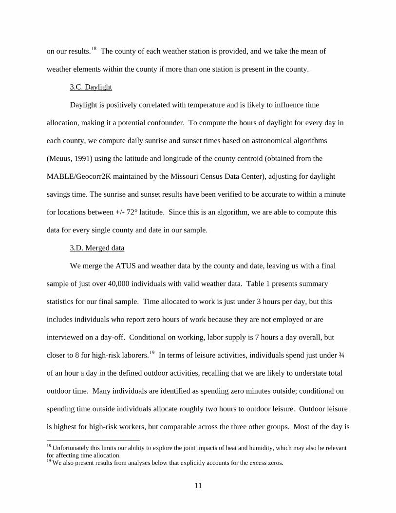
A potential concern with the ATUS is non-response – not all individuals selected for the
ATUS agree to participate, and this may bias our analysis. While others have assessed the
degree of non-response bias with respect to socio-demographic factors (Abrams et al. 2006), a
particularly relevant concern in this context is that temperature may affect whether an individual
participates in the survey. Because the weather data applies to the universe of observations, we
can assess whether temperature is related to survey participation by plotting the distribution of
temperature for counties in our final sample for both the days time diaries are available and the
days time diaries are unavailable. Shown in Appendix Figure 1, the distribution of temperature
across the two groups is nearly identical, suggesting non-response bias due to temperature is
likely to be minimal in our analysis.
An additional concern is that the external validity of our sample is compromised by only
focusing on more urban areas where geographic residence is obtained. To examine this issue, we
also plot the temperature distribution for counties that are not included in the ATUS for the same
dates as ATUS respondents’ diaries. Also shown in Appendix Figure 1, we find little difference
between the two distributions, suggesting external validity is unlikely to be compromised.
4. Econometric Model
4.A. Baseline model
To examine the relationship between temperature and time allocation, we estimate the
following econometric model:
(1) plaborict = ∑jβ1j tempct + δ1Zct + γ1Xic + DOW1t + f1(t) + α1c + ε1ict
(2) poutdoorict = ∑jβ2j tempct + δ2Zct + γ2Xic + DOW2t + f2(t) + α2c + ε2ict
13
(3) pindoorict = ∑jβ3j tempct + δ3Zct + γ3Xic + DOW3t + f3(t) + α3c + ε3ict
(4) β1j + β2j +β3j = 0 for all j
where plabor is the percent of time allocated to labor market activities for individual i in county
c on date t, poutdoor is the percent of time allocated to outdoor leisure activities, and pindoor is
the percent of time allocation to indoor leisure activities.22 Temp are dummy variables that
flexibly model the relationship between daily maximum temperature and time allocation,
described below. Zct are other environmental attributes potentially correlated with temperature
(daylight, precipitation, humidity, and minimum temperature) and Xic are individual level
covariates meant to capture preferences for particular activities, listed in Table 1. DOWt are day
of week dummy variables to account for differences in schedules throughout the week. f(t) are
year-month dummy variables to control for seasonal and annual time trends in activity choice. αc
are county fixed effects that capture all time invariant observable and unobservable attributes
that affect time allocation decisions. Therefore, our parameters of interest that relate temperature
to time (βj) are identified from daily variations in weather within a county. We demonstrate
below that our results are insensitive to numerous robustness checks, supporting the validity of
our model.23
We estimate equations (1)-(3) via seemingly unrelated regression, imposing constraint
(4), which limits the net effect from a temperature change on total time to sum to zero.24 For
ease of interpretation, we multiply all coefficients by the total number of minutes in a day (1440)
to obtain the change in minutes allocated to each activity. We estimate these models for all
individuals, and then separately for those employed in high-risk industries and those employed in
22 Note that we do not distinguish between home production and leisure. 23 Since multiple individuals can be observed on the same day within a county, we cluster standard errors on the county-date. 24 We assess the impact of this restriction below.
14

low-risk industries. For those not currently employed, we estimate equations (2)-(3), modifying
the constraints accordingly.
To examine the impacts of temperatures, it is essential that we flexibly model the
relationship between temperature and time spent in certain activities given the expected
nonlinear relationship: increases in temperature may lead to increases in outdoor leisure at colder
temperatures, but beyond a certain point may lead to decreases (Galloway and Maughan, 1997).
Our model includes separate indicator variables for every 5-degree temperature increment (as
displayed in Figure 1), which allows differential shifts in activities for each temperature bin.25
We omit the 76-80 degree indicator variable, so we interpret our estimates as the change in
minutes allocated to that activity at a certain temperature range relative to 76-80 degrees.
4.B. Exploring adaptation
We estimate several alternative models to explore the scope for behavioral substitutions
and acclimatization, with the mean of the dependent variables for these alternative models shown
in Table 2. To assess intertemporal substitution, we include lagged temperature in equations (1)-
(3) in addition to contemporaneous temperature, and also place a comparable constraint on
lagged temperatures that the net effect on total time sums to zero. We also flexibly model lagged
temperature using the same indicator variables. Since people may not be able to substitute across
immediately adjacent days, we specify lagged temperature as the maximum temperatures across
the previous six days. If individuals substitute activities across days, then we expect unpleasant
lagged temperatures to increase the demand for current activities.
By aggregating responses within a day, any estimated effects are net of intratemporal
substitutions whereby individuals reschedule activities to more pleasant times of the day. To
25 Models with 2.5 degree size bins for temperature yield strikingly similar results. We also estimated models with higher order polynomials in temperature. Our results were sensitive to the polynomial degree (results available upon request), thus persuading us to use a more flexible approach.
15

assess intratemporal substitution, we split the dependent variables in equations (1)-(3) into time
spent during daylight vs. twilight hours and estimate separate models for each. To define time
allocation during twilight, we include activities that began less than two hours after sunrise or
less than two hours before sunset, where sunrise and sunset values vary over both space and
time. Since we are interested in comparing daylight vs. twilight responses and the mean level of
each variable differs (as shown in Table 2), we present these results as the percentage change in
time allocation by dividing the change in minutes by the mean of the dependent variable. If
unpleasantly warm days are cooler during the evening or the morning, then we expect smaller
responses to temperatures during twilight hours as compared to daylight hours.
The impacts of short-run acclimatization are assessed by estimating separate temperature
responses for June and August. Since hot days are a relatively new phenomenon in June but
quite common by August, a diminished response to high temperatures in August should be
viewed as evidence of acclimatization.26 Since this test greatly reduces our sample size and
power to detect differential effects, we modify the minimum temperature bin to under 65
degrees, a reasonably innocuous change given the months of our focus.
By including county fixed effects, the econometric model identifies short run behavioral
responses to temperature. Although most physiological acclimatization occurs within a short
period of time, behavioral acclimatization may require more time to take effect. To assess longer
run adjustments, we explore the impacts of temperature separately for historically warmer and
cooler areas. In particular, we compare the response function for people that live in places with
the warmest third of average July-August temperatures during the 1980s to those that lived in the
26 We do not want to conduct this test by comparing the impact of temperature across seasons for at least two reasons. One, this only identifies impacts where there is sufficient temperature overlap across seasons, making it unlikely to identify the impact from very hot weather. Two, marginal utility from pleasant weather may diminish at different rates depending on how often such weather is experienced.
16

coldest third.27 The presumption is that those that live in hotter climates have had longer periods
of time to adapt to warmer conditions, through more complete physiological adaptation as well
as investments in technologies that make it easier to cope with high temperatures. If people
adapt to changes in climate, people in cooler places would show comparable adaptations as they
become warmer, suggesting that the short run response curve of colder places will eventually
become like the short-run response curve of hotter places.
5. Results
5.A. Baseline results
We begin with a focus on the impacts of temperature on time allocation for all
individuals, and then focus on the impacts for the groups defined in Table 1. In Figure 2, we find
some evidence of a downward trend in labor supply from higher temperatures, shown in the first
panel. The estimates, however, are not large in magnitude – the response at 100+ degrees is 19
minutes – and are not statistically significant at conventional levels. This suggests that,
consistent with recent findings (Connolly, 2008), labor supply on net is not responsive to
changes in temperature.
Turning to leisure time, we find an asymmetric relationship between temperature and
outdoor leisure. Time outside at 25 degrees is 37 minutes less than at 76-80 degrees, and
steadily climbs until 76-80 degrees. It remains fairly stable until 100 degrees, and falls after that,
though the impact at the highest temperature bin is not statistically significant. While this pattern
is consistent with physiological evidence suggesting fatigue from exposure at temperature
27 The colder places predominantly consist of counties in the Northeast and upper Midwest; warmer places in the Southeast and Southwest; and omitted places in the mid-Atlantic, mountain states, and lower Midwest. California was almost evenly split amongst the three categories. We also perform this analysis for those in the warmest/coldest quartile or quintile, and found comparable results.
17

extremes (Galloway and Maughan (1997), the lack of significance at high temperatures and the
high inflection point suggests external factors may play an important role in individuals
responses.
Indoor leisure shows a highly asymmetric U-shaped pattern. Indoor leisure increases by
roughly 30 minutes at 25 degrees compared to 76-80 degrees, and then steadily decreases until
76-80 degrees. It remains stable until roughly 95 degrees, and then increases considerably after
that. At temperatures over 100 degrees, indoor leisure increases by 27 minutes relative to 76-80
degrees, with this estimate statistically significant at conventional levels.
The analysis in Figure 2, however, masks potentially important heterogeneity due to
differential occupational exposure to temperature. In Figure 3, we focus on time allocations for
individuals employed in industries with a high risk of climate exposure. For labor supply, we
continue to find little response to temperatures below 80 degrees, but monotonic declines in
labor supply above 85 degrees. At temperatures over 100 degrees, labor supply drops by a
statistically significant 59 minutes as compared to 76-80 degrees. Thus, as hypothesized, the
marginal productivity of labor for these workers appears to be significantly impacted by
temperatures at the high end of the climate spectrum.
In terms of leisure activities, the results are comparable to the patterns found for all
workers, with a slightly higher increase in indoor leisure to accommodate the decrease in labor
supply at higher temperatures. At high temperatures, workers appear to substitute their labor
supply for indoor leisure, with surprisingly no decline in outdoor leisure. This suggests that,
while the marginal utility from outdoor leisure may be declining, the marginal utility of indoor
leisure is decreasing at a faster rate over this temperature range.
18

In Figure 4, we focus on time allocations for those in low-risk industries. For labor
supply, we again see little response to colder temperature. While we see a decrease in labor
supply at temperatures above 95 degrees, this effect is modest and not statistically significant.
The high fraction of workers in these industries explains why we see no net effect on labor
supply from higher temperatures. In terms of leisure activities, we see comparable responses as
above for colder temperatures, but more muted responses at hotter temperatures which is
consistent with the smaller labor supply response for this group.
In Figure 5, we present results for those not employed. Consistent with expectations, we
find outdoor and indoor leisure more responsive to temperature changes, particularly at hotter
temperatures. Outdoor leisure begins decreasing at lower temperatures when compared to
employed individuals, with declines beginning around 90 degrees. Furthermore, the impacts at
higher temperatures are larger and statistically significant. Temperatures over 100 degrees lead
to a statistically significant decrease in outdoor leisure of 22 minutes compared to 76-80 degrees.
Consistent with Deschenes and Greenstone (2007b), such responses at high temperatures are
supportive of short-run adaptation whereby individuals protect themselves from the heat by
spending more time inside, which may lessen the health impacts from higher temperatures
(Alberini et al., 2008).
5.B. Robustness checks
In Figure 6, we display results from models that assess the sensitivity of our results to
several specification checks, though our results are robust to additional checks not shown. We
focus solely on labor supply for high-rsk workers and outdoor leisure for non-employed because
this is where we find the largest and most significant effects, though results are similar for the
other activities and groups shown in Figures 2-5. We include in this figure the confidence
19

intervals from our baseline results to facilitate interpretation, though as we demonstrate below
our estimates are highly insensitive to these alternate specifications.
Since those employed in the manufacturing industry may in fact work in low risk
industries if the manufacturing plant is climate controlled, we may have erroneously classified
exposure risk for some workers. Our first robustness check shifts individuals from the
manufacturing industry into low risk.28 Despite the nearly 50% decrease in sample size in the
high risk group, our estimates are largely unaffected by this change. If anything, we find a
slightly larger reduction in labor supply at higher temperatures, which is consistent with this
misclassification, though the difference is minimal.
In the next two checks we assess potential omitted variable bias. First, we exclude all
individual level covariates to assess whether county fixed effects capture sorting into locations
based on temperature. Second, we include county-season fixed effects to allow for seasonal
shocks specific to each county. Figure 6 confirms that these modifications have minimal impact
on our estimates, suggesting confounding is unlikely to be a major concern.
As previously mentioned, we have a large mass of observations at zero. Since these
zeros represent corner solutions rather than a negative latent value, linear models should produce
consistent estimates of the partial effects of interest near its mean value. To further assess this,
we estimate two-part models that separately model the extensive and intensive margins.29 In
estimating this model, we also relax the constraint that the coefficients across activities sum to
zero, so it also tests this restriction. Shown in this Figure, the results from the two-part model
28 This test is irrelevant for the non-employed group. 29 More specifically, based on laws of probability, E(y|x) = P(y>0|x) * E(y|y>0,x). We estimate P(y>0|x) using a probit model and E(y|y>0,x) by OLS, and compute marginal effects by taking the derivative of P(y>0|x) * E(y|y>0,x).
20

are quite comparable to the linear estimates. Taken together, the results from Figure 6 document
a robust relationship between temperature and time allocation.
5.C. Adaptation
Our static, short-run model may conceal important responses that minimize the impact of
climate shocks. In this section, we probe potential behavioral substitutions and acclimatization
as described in the econometric section. As with the robustness checks, we focus solely on labor
supply for high-risk workers and outdoor leisure for non-employed because this is where we find
the largest effects and hence have the largest scope for adaptation. It is important to keep in mind
that these tests rely on considerably smaller sample sizes, particularly at the upper tail of the
distribution, and thus are underpowered to produce statistical significance at conventional levels.
Given the importance of this topic and the inherently limited data availability under current
climatic conditions, these results should be viewed as suggestive of the types of adaptation we
may see in the future.
We begin by exploring the intertemporal effects of temperature whereby individuals may
compensate for unpleasant weather by shifting their activities across days, suggesting that the
estimates we have shown thus far may overstate the impacts from warmer temperatures. In
Figure 7 we present estimates from regressions that includes the same indicator variables for
lagged temperature (in addition to indicators for current temperature). Given that we find a
decrease in labor supply for high-risk workers, if intertemporal substitution exists we expect to
see an increase in labor supply from high lagged temperatures. This does not appear to be the
case, suggesting little or no role for intertemporal substitution in the workplace. In contrast,
outdoor leisure for the non-employed appears responsive to rescheduling. The two highest
21

temperature bins for lagged temperature are positive, with the estimate of an increase of 15
minutes at 100+ degrees (compared to 76-80 degrees) statistically significant at the 10% level.
In Figure 8, we present results exploring the potential for intratemporal substitution by
estimating whether individuals shift the timing of activities within the day. For labor supply, we
find that hours worked during daylight is largely unaffected by warmer temperatures. However,
hours worked during twilight is highly responsive to warmer temperatures, and hence appears to
be the driving force behind the labor supply response found in our base analyses. Furthermore,
the difference in responses for temperatures above 85 degrees is statistically significant at
conventional levels. If we separate twilight time into the beginning vs. end of the day (not
shown), we also find that nearly all of the decrease during twilight hours comes from the end of
the day. This pattern is consistent with the idea that workers have little discretion over labor
supply during core business hours, but as fatigue sets in from accumulated exposure to higher
temperatures and marginal productivity declines, labor supply becomes responsive.
Turning to outdoor leisure for the non-employed, we find patterns consistent with
individuals shifting activities to more favorable times of the day, though the differences are not
statistically significant. For example, we find the turning point for twilight activities occurs at
higher temperatures. Furthermore, the drop off from temperatures above 100 degrees is smaller
during twilight hours, representing a 26 percent decrease as opposed to a 58 percent decrease
during daylight hours (compared to 76-80 degrees).
As a test of short-run acclimatization, we explore whether individuals are less sensitive to
warmer temperatures as they become more common by estimating the impact of temperatures
separately in June vs. August. While our estimate for the highest temperature bin is consistent
with acclimatization for labor supply, the overall pattern is less well-behaved. For outdoor
22

leisure, we find a pattern highly consistent with short-run acclimatization. Responses in August
compared to June are smaller at high temperatures but larger at unseasonably cold temperatures.
Given the dramatic drop in sample size, it is unsurprising that these differences are not
statistically significant. The differences at high temperatures, however, are large in magnitude.
For example, at days over 100 degrees, the non-employed spend 30 more minutes outside in
August than in June.
Thus far we have assumed that all individuals respond to temperatures in the same way.
Our final test for adaptation allows for heterogeneous responses to temperature based on
historical climates by grouping counties into those in the highest third of historical July-August
temperatures and the coldest third. Shown in Figure 10, although we continue to see declines in
both labor supply and outdoor leisure at high temperatures in the historically warmer places, the
response to high temperatures, particularly for outdoor leisure, is noticeably smaller than the
response in colder places. Here again the difference in estimates is not statistically significant
but the point estimates are quite large.
6. Conclusion
The warmer temperatures that are projected to spread across the planet are likely to have
significant impacts on our daily lives, so understanding how individuals respond to these changes
is essential for the design of well-formulated policies. In this paper, we examine the impacts of
climate on individual’s allocation of time within the US. We find large reductions in labor
supply in climate-exposed industries as temperatures increase beyond 85 degrees. We also find
large decreases in outdoor leisure activities at higher temperatures, but only for those who are not
employed.
23

Our labor results imply a substantial transfer of income from mostly blue-collar sectors
of the economy to more white-collar sectors, which may have important regional and political
consequences. Moreover, the restructuring of leisure time in response to climate change carries
with it substantial welfare implications. Nearly $300B per year is spent on outdoor recreational
activities alone (American Recreation Coalition, 2007), so summer reductions in outdoor time
represent a direct and potentially large loss of utility while winter increases could bring gains.
Similarly, substitution toward or away from sedentary activities as seasonal temperatures move
in and out of the comfortable range could have profound impacts on population health through
changes in the incidence of obesity, diabetes, and cardiovascular disease.30
It is also important to note that while the net employment impacts in the US may be
small, they may be considerably larger in developing countries, where the industrial base is more
typically concentrated in climate-exposed industries and baseline temperatures are already
warmer. In middle-income countries like Mexico, for example, back-of-the-envelope
calculations suggest a 2.0% drop in overall employment at the end of this century.31 In poorer
regions like sub-Saharan Africa, where nearly all labor is in climate-exposed industries, the
consequences may be devastating. Such a pattern of results is strikingly consistent with the
emerging literature on climate change and macroeconomic growth (Dell et al., 2008).
While we find suggestive evidence of adaptation through temporal substitutions and
acclimatization, it is likely that adaptation will become more substantial in the future. Better
technologies to cope with the elements will be invented and firms may find their adoption
30 See, for example, Veerman et al., 2007, Li et al., 2006, and Laaksonen et al., 2005. 31 We compute these numbers by assuming the labor supply response in Mexico is the same as the US, using Texas baseline temperatures for Mexico, imposing a uniform warming of 5 degrees Celsius, and assuming 49.7% are employed in exposed industries (Hanson, 2003). Clearly labor supply responses may differ, especially if the rate of substitution between capital and labor differs and/or capital is differentially affected by climate change. While a time use survey for Mexico is available (Encuesta Nacional sobre Trabajo, Aportaciones y Uso del Tiempo), it does not include the necessary variables to permit such an analysis.
24

increasingly attractive as the costs associated with lost labor productivity become larger.
Adaptation may also take the form of re-location if individuals and firms move from the
currently warm regions of the South to the historically cooler North.32 Similar changes may take
place on a global scale. Exploring the scope for longer-run adaptation is essential for policy
making and a fruitful area for future research.
32 Previous research examining climate and migration have typically focused on moving away from colder weather (e.g., Cragg and Kahn, 1997; Deschenes and Moretti, 2009), which is sensible given historical patterns in climate and the gradual shifting of population towards the South and Southwestern regions of the US. But we could conceivably begin to see reverse patterns as people seek to avoid heat, especially as the colder winters in Northern regions becomes milder.
25

References
Abrams, Katharine, Aaron Maitland, and Suzanne Bianchi (2006). “Nonresponse in the American time use survey: Who is missing from the data and how much does it matter?” Public Opinion Quarterly 70(5): 676–703.
Alberini, Anna, Erin Mastrangelo and Hugh Pitcher (2008). “Climate Change and Human Health: Assessing the Effectiveness of Adaptation to Heat Waves.” Mimeograph, University of Maryland
Albouy, David, Walter Graf, Ryan Kellogg, and Hendrik Wolff, “The Impact of Climate Change on Household Welfare.” Mimeo, University of Michigan.
American Recreation Coalition (2007). “Outdoor recreation outlook 2008.” Prepared for the 2007 Marketing Outlook Forum.
Armstrong, LE and CM Maresh (1991). “The induction and decay of heat acclimatization in trained athletes.” Sports Med. 12: 302-312.
Biddle, Jeff and Daniel Hamermesh (1990). “Sleep and the Allocation of Time.” Journal of Political Economy 98(5): 922-43.
Connolly, Marie (2008). “Here Comes the Rain Again: Weather and the Intertemporal Substitution of Leisure.” Journal of Labor Economics 26(1): 73-100.
Cragg, Michael and Matthew Kahn (1997). “New Estimates of Climate Demand: Evidence from Location Choice.” Journal of Urban Economics 42: 261-284.
Dell, Melissa, Benjamin Jones and Benjamin Olken (2008). “Climate Change and Economic Growth: Evidence from the Last Half Century.” NBER Working Paper 14132.
Deschenes, Olivier and Michael Greenstone (2007a), “The Economic Impacts of Climate Change: Evidence from Agricultural Output and Random Fluctuations in Weather,” American Economic Review 97(1): 354-385. Deschenes, Olivier and Michael Greenstone (2007b). “Climate Change, Mortality, and Adaptation: Evidence from Annual Fluctuations in Weather in the US.” NBER Working Paper 13178.
Deschenes, Olivier and Enrico Moretti (2009). “Extreme Weather Events, Mortality and Migration.” Review of Economics and Statistics, forthcoming. Eisenberg, D, and E Okeke (2009). “Too Cold for a Jog? Weather, Exercise, and Socioeconomic Status.” B.E. Journal of Economic Analysis & Policy 9(1) (Contributions): Article 25.
Englin, Jeffrey, and Klaus Moeltner (2004). “The Value of Snowfall to Skiers and Boarders,” Environmental and Resource Economics 29:123-136.
Epstein Y, Keren G, Moisseiev J, Gasko O, Yachin S. (1980). “Psychomotor deterioration during exposure to heat.” Aviat Space Environ Med. 51(6): 607-10.
Galloway SD, Maughan RJ (1997). “Effects of ambient temperature on the capacity to perform prolonged cycle exercise in man.” Med Sci Sports Exerc. 29(9): 1240-9.
González-Alonso, José, Christina Teller, Signe L. Andersen, Frank B. Jensen, Tino Hyldig, and Bodil Nielsen (1999). “Influence of body temperature on the development of fatigue during prolonged exercise in the heat.” J Appl Physiol 86: 1032-1039.
Hancock PA, Ross JM, Szalma JL. (2007). “A meta-analysis of performance response under thermal stressors.” Hum Factors 49(5): 851-77.
Hanson, Gordon (2005). “What Has Happened to Wages in Mexico since NAFTA?” NBER Working Paper 9563.
26

Laaksonen DE, J Lindstrom, TA Lakka, et al. (2005). “Physical activity in the prevention of type 2 diabetes: the Finnish diabetes prevention study.” Diabetes 54(1):158-65.
Li TY, JS Rana, JE Manson, et al. (2006). “Obesity as compared with physical activity in predicting risk of coronary heart disease in women.” Circulation 113(4):499-506.
Loomis, John and John Crespi (1999). “Estimated Effects of Climate Change on Selected Outdoor Recreation Activities in the United States,” Chapter 11 in The Impact of Climate Change on the United States Economy, Cambridge University Press, pp. 289-314.
Ma, Y, BC Olendzki, W Li, AR Hafner, D Chiriboga, JR Hebert, M Campbell, M Sarnie and IS Ockene (2006). “Seasonal variation in food intake, physical activity, and body weight in a predominantly overweight population.” European Journal of Clinical Nutrition 60: 519–528.
Mendelsohn, R., W. Nordhaus and D. Shaw (1994). ”The Impact of Global Warming on Agriculture: A Ricardian Approach”, American Economic Review 84(4): 753-771.
Mendelsohn, Robert and Marla Markowski (1999). “The Impact of Climate Change on Outdoor Recreation,” Chapter 10 in The Impact of Climate Change on the United States Economy, Cambridge University Press, pp. 267-288.
Nielsen, B, J R Hales, S Strange, N J Christensen, J Warberg and B Saltin (1993). “Human circulatory and thermoregulatory adaptations with heat acclimation and exercise in a hot, dry environment.” J Physiol Vol 460: 467-485.
NIOSH (1986). “Working in Hot Environments.” NIOSH Publication No. 86-112. Nordhaus, William (2006). “Geography and Macroeconomics: New Data and Findings,”
Proceedings of the National Academy of Science 103: 3510-3517. Pilcher JJ, Nadler E, Busch C. (2002). “Effects of hot and cold temperature exposure on
performance: a meta-analytic review.” Ergonomics 45(10): 682-98. Pivarnik, J. M., Reeves, M. J., Rafferty, A. P. (2003). “Seasonal variation in adult leisure-
time physical activity.” Med Sci Sports Exerc 35: 1004–1008. Rabin, M. (1998). “Psychology and economics.” Journal of Economic Literature, 36(1):
11-46. Ramsey JD. (1995). “Task performance in heat: a review.” Ergonomics 38(1): 154-65. Sachs, Jeffrey D. and Andrew Warner (1997). “Sources of Slow Growth in African
Economies,” Journal of African Economies, 6: 335-76. Schlenker, Wolfram, W. Michael Hanemann, and Anthony Fisher (2005), “Will U.S.
Agriculture Really Benefit from Global Warming? Accounting for Irrigation in the Hedonic Approach,” American Economic Review 95(1), pp. 395-406.
Schlenker, Wolfram, and Michael Roberts (2008). “Estimating the Impact of Climate Change on Crop Yields: The Importance of Nonlinear Temperature Effects.” NBER working paper 13799.
Wagner, JS, AS Robinson, SP Tzankoff, and RP Marino (1972). “Heat tolerance and acclimatization in the heat in relation to age.” Journal of Applied Physiology, 33(5): 616-622.
Veerman JL, Barendregt JJ, van Beeck EF, et al. (2007). “Stemming the obesity epidemic: a tantalizing prospect.” Obesity 15(9):2365-70.
27

Figure 1. Historical and forecasted temperature distribution
02
468
1012
1416
<30
31-35
36-40
41-45
46-50
51-55
56-60
61-65
66-70
71-75
76-80
81-85
86-90
91-95
96-10
010
0+
2003-06 2070-2099
Notes: This figure is based on daily observations for each county included in the final ATUS sample for the years indicated. 2070-2099 forecasted temperatures are based on the Hadley 3 climate model under the highest warming scenario (A1).
28

Figure 2. Relationship between temperature and time allocation for all individuals -8
0-6
0-4
0-2
00
2040
6080
2535
4555
6575
8595
105 2535
4555
6575
8595
105 2535
4555
6575
8595
105
Labor Outdoor Indoor
min
utes
maximum temperature (°F)
Notes: N=42,280 in all regressions. 95% confidence interval shaded in gray. Each figure displays the estimated impact of temperature on time allocation based on equations (1)-(4) in the text. Covariates include age, gender, # of children, earnings, employment status, race, education, marital status, family income, day of week dummies, minimum temperature, precipitation, humidity, sunrise, sunset, year-month dummies, and county fixed effects.
29

Figure 3. Relationship between temperature and time allocation for high risk industries -8
0-6
0-4
0-2
00
2040
6080
2535
4555
6575
8595
105 2535
4555
6575
8595
105 2535
4555
6575
8595
105
Labor Outdoor Indoor
min
utes
maximum temperature (°F)
See notes to Figure 2. N=6,246 in all regressions. 95% confidence interval shaded in gray. ‘High risk’ defined as agriculture, forestry, fishing, and hunting, mining, construction, manufacturing, and transportation and utilities industries.
30

Figure 4. Relationship between temperature and time allocation for low risk industries -8
0-6
0-4
0-2
00
2040
6080
2535
4555
6575
8595
105 2535
4555
6575
8595
105 2535
4555
6575
8595
105
Labor Outdoor Indoor
min
utes
maximum temperature (°F)
See notes to Figure 2. N=21,151 in all regressions. 95% confidence interval shaded in gray. ‘Low risk’ defined as remaining industries not listed in Figure 3.
31

Figure 5. Relationship between temperature and time allocation for non-employed -8
0-6
0-4
0-2
00
2040
6080
2535
4555
6575
8595
105 2535
4555
6575
8595
105
Outdoor Indoor
min
utes
maximum temperature (°F)
See notes to Figure 2. N=14,883 in all regressions. 95% confidence interval shaded in gray. ‘Non-employed’ defined as unemployed or out of labor force.
32

Figure 6. Robustness checks -1
20-1
00-8
0-6
0-4
0-2
00
2040
6080
2535
4555
6575
8595
105 2535
4555
6575
8595
105
High-risk, labor Non-employed, outdoor
+/-manufcaturing w/o ind. cov.county-season FE two-part model
min
utes
maximum temperature (°F)
See notes to Figure 2. 95% confidence interval for baseline estimates shaded in gray. ‘+/- manufacturing’ moves those employed in the manufacturing industry from high to low risk. ‘w/o ind. cov.’ excludes all individual level covariates. ‘county-season FE’ includes a county-season fixed effect. ‘two-part model’ presents marginal effects from models that separately estimate the extensive and intensive margins to account for excess zeros and does not constrain coefficients across activities to sum to zero.
33

Figure 7. Intertemporal substitution -8
0-6
0-4
0-2
00
2040
2535
4555
6575
8595
105 2535
4555
6575
8595
105
High-risk, labor Non-employed, outdoor
lagged contemporaneous
min
utes
maximum temperature (°F)
See notes to Figure 2. Estimates include indicator variables for both contemporaneous temperature and lagged temperature, where lagged temperature is defined as the maximum of the 6 previous days’ temperature. 95% confidence interval for lagged estimates shaded in gray.
34

Figure 8. Intratemporal substitution
-100
-80
-60
-40
-20
020
2535
4555
6575
8595
105 2535
4555
6575
8595
105
High-risk, labor Non-employed, outdoor
daylight twilight
perc
ent
maximum temperature (°F)
See notes to Figure 2. “Daylight” is defined as the time from 2 hours after sunrise until 2 hours before sunset. “Twilight” is defined as before 2 hours after sunrise or after 2 hours before sunset.
35

Figure 9. Short-run acclimatization -1
50-1
00-5
00
5010
015
020
025
0
6070
8090
100 6070
8090
100
High-risk, labor Non-employed, outdoor
June August
min
utes
maximum temperature (°F)
See notes to Figure 2. Results from this figure are based on regressions stratified by month. N=483 for “June” estimates and N=477 for “August” estimates for high risk. N=1173 for “June” estimates and N=1228 for “August” estimates for non-employed.
36

Figure 10. Medium-run acclimatization -1
20-1
00-8
0-6
0-4
0-2
00
2040
2535
4555
6575
8595
105 2535
4555
6575
8595
105
High-risk, labor Non-employed, outdoor
warm cool
min
utes
maximum temperature (°F)
Notes: See notes to Figure 2. Results from this figure are based on regressions stratified by historical climate. Warm (cool) is defined as counties in the top (bottom) third of the 1980-1989 July-August temperature distribution. N=2066 (2364) for warm (cool) July-August in high risk industries. N=5365 (5102) for warm (cool) July-August non-employed.
37

Table 1. Summary statistics All
(N=42280) High-risk (N=6246)
Low-risk (N=21151)
Non-employed
(N=14883) Mean SD Mean SD Mean SD Mean SD A. Time allocation Labor hours 2.71 4.05 4.38 4.58 4.06 4.34 - - percent hours = 0 0.61 0.49 0.43 0.5 0.42 0.49 - - hours | hours > 0 7.01 3.51 7.76 3.3 6.99 3.46 - - Outdoor leisure hours 0.73 1.61 0.99 2.09 0.65 1.48 0.73 1.55 percent hours = 0 0.6 0.49 0.6 0.49 0.61 0.49 0.58 0.49 hours | hours > 0 1.82 2.12 2.47 2.7 1.67 1.99 1.75 1.98 Indoor leisure hours 11.72 3.86 10.13 3.82 10.7 3.83 13.80 2.82 B. Covariates max. temperature (˚F) 67.48 19.04 67.01 18.92 67.31 19.18 67.91 18.88 min. temperature (˚F) 47.16 17.57 46.52 17.24 47.03 17.73 47.61 17.47 precip. (in./100) 11.17 30.23 11.09 28.95 10.83 29.5 11.70 31.77 snowfall (in./10) 0.66 5.17 0.69 4.88 0.64 4.87 0.67 5.66 max. rel. humidity 84.68 14.22 84.9 13.93 84.67 14.2 84.60 14.38 age 45.29 17.25 42.32 11.47 41.34 13.39 52.16 21.50 male 0.43 0.5 0.74 0.44 0.41 0.49 0.34 0.47 # children < 18 0.92 1.16 1.03 1.17 0.98 1.13 0.79 1.19 annual earnings ($1k) 46.0 61.2 80.3 62.2 68.2 63.3 - - diary day a holiday 0.02 0.13 0.02 0.14 0.02 0.13 0.02 0.13 employed 0.65 0.48 - - - - - - absent from work 0.03 0.17 0.04 0.2 0.04 0.21 - - out of labor force 0.31 0.46 - - - - 0.88 0.33 employed full time 0.51 0.5 0.91 0.29 0.75 0.43 - - white non-Hispanic 0.68 0.47 0.69 0.46 0.7 0.46 0.66 0.47 HS dropout 0.17 0.38 0.13 0.34 0.1 0.3 0.29 0.45 HS graduate 0.25 0.43 0.33 0.47 0.2 0.4 0.29 0.45 some college 0.26 0.44 0.28 0.45 0.28 0.45 0.22 0.42 spouse/partner in HH 0.55 0.5 0.68 0.47 0.57 0.49 0.47 0.50 Notes: All statistics at the daily level. ‘High risk’ defined as those employed in agriculture, forestry, fishing, and hunting, mining, construction, manufacturing, and transportation and utilities industries. ‘Low risk’ consists of remaining industries. ‘Non-employed’ defined as unemployed or out of labor force.
38

Table 2. Various labor and outdoor leisure measures All High risk Low risk Non-
employed Intratemporal substitution Labor: twilight 1.31 2.25 1.92 - Labor: daylight 1.38 2.08 2.10 - Outdoor leisure: twilight 0.24 0.36 0.22 0.23 Outdoor leisure: daylight 0.48 0.63 0.43 0.51 N 42280 6246 21151 14883 By historical July-August temperature Labor: warm 2.68 4.49 4.14 0.08 Outdoor leisure: warm 0.71 0.98 0.61 0.74 Labor: cold 2.72 4.20 4.01 0.10 Outdoor leisure: cold 0.76 1.02 0.69 0.74 N 15058 2364 7592 5102 By month Labor: June 2.69 4.58 3.94 0.13 Outdoor leisure: June 1.00 1.24 0.91 1.03 Labor: August 2.75 4.25 4.16 0.08 Outdoor leisure: August 0.94 1.19 0.86 0.98 N 3527 477 1822 1228 Note: All numbers represent the mean value of each variable for each group. “Daylight” is defined as the time from 2 hours after sunrise until 2 hours before sunset. “Twilight” is defined as before 2 hours after sunrise or after 2 hours before sunset. Warm (cool) is defined as counties in the top (bottom) third of the 1980-1989 July-August temperature distribution.
39
Appendix Figure 1: Distribution of observations by temperature for excluded and included sample
02468
101214
<30
31-35
36-40
41-45
46-50
51-55
56-60
61-65
66-70
71-75
76-80
81-85
86-90
91-95
96-10
010
0+
maximum temperature
perc
ent o
f day
s
ATUS ATUS non-response Counties not in ATUS
Notes: ‘ATUS’ is the final sample used in the analysis. ‘ATUS non-response’ is the same counties as the final sample but on dates without time diaries. ‘Counties not in ATUS’ is all dates from counties not included in the ATUS sample.
40