tensor analysis applied to the equations of continuum ... · tensor analysis applied to the...

Tensor analysis applied to the equations of continuum mechanics I

FFI-rapport 2013/02772

Øyvind Andreassen

ForsvaretsforskningsinstituttFFI

N o r w e g i a n D e f e n c e R e s e a r c h E s t a b l i s h m e n t


Tensor analysis applied to the equations of continuum mechanics I

Øyvind Andreassen

Norwegian Defence Research Establishment (FFI)

27 January 2014


131101

P: ISBN 978-82-464-3210-4E: ISBN 978-82-464-2311-1

Keywords

Tensor analyse

Sylinder koordinater

Generaliserte koordinater

Fluid ligningene

Lighthill’s ligning

RANS ligningene

Approved by

Bjørn Anders Pettersson Reif

Jan Ivar Botnan

Project manager

Director

FFI-rapport 2013/02772 2

English summary

The Navier-Stokes equations, the Euler equations, the equations of elasticity and expressions

derived from those, are in most cases treated in Cartesian coordinates. In some cases it can

necessary to handle those equations in other coordinate systems. In the cases of cylindrical

coordinates, for example in the description of the flow around acoustic antennas, it is natural

to use cylinder coordinates. In this report, we present the formalism necessary to handle the

mentioned equations and related expressions in generalized coordinates. The formalism include

tensor analysis, developed during 1850-1900 by Gregorio Ricci Kurbastro, Tullio Levi-Civita,

Sophus Lie and others. Albert Einstein used tensor analysisas the mathematical basis for the

General Theory of Relativity. In this report we will limit our self to describe the classical fluid

equations in generalized coordinates.

The tensor-theory can appear to be difficult and one can ask ifit is necessary to go through

all these complicated calculations. Can’t they be found at the web or in standard collections

of formulas? We have looked for expressions, for example∇ · (∇(ρT)), whereT is the mo-

mentum flux density tensor that appears in Lighthill’s equation. We could not find this derived

in cylinder coordinates and it was necessary to calculate itby hand to achieve our goals. In

the analysis of flow around an acoustic antenna, various tensors appear, for example the strain

rate tensor, structural tensors and tensorial expressionsinvolved in the RANS equations, it was

necessary to follow the formalism of tensor analysis in detail.

With data given in cylinder coordinates, it is natural to do the analysis also in cylinder coordi-

nates. Physical components of both vectors and tensors are used in the physical interpretations

of the data.

Although the treatment in cylinder coordinates addressed in this report only is directly ap-

plicable to a limited number of applications, the concept oftensor analysis is fundamental in

practically all applications of continuum mechanics.


Sammendrag

Navier-Stokes ligninger, Euler ligningene og elastisitets ligningene og uttrykk avledet av disse

handteres oftest i Cartesiske koordinater. Det kan likevel være avgjørende a kunne handtere

disse ligningene i andre koordinatsystemer, for eksempel isylinder-koordinater i tilfellet

strømning omkring eller i cylindriske rør, for eksempel strømning rundt akustiske antenner.

I dene rapporten presenterer vi formalismen som ma til for ˚a uttrykke de nevnte ligningene i

generaliserte koordinater. Formalismen omfatter tensoranalyse, som ble utviklet i tidsrommet

1850-1900 av Gregorio Ricci Kurbastro, Tullio Levi-Civita, Sophus Lie og andre. Albert Ein-

stein benyttet tensor analysen som som matematisk fundament for generell relativitetsteori. I

denne rapporten vil vi begrense oss til a beskrive de klassiske fluid ligningene i generaliserte

koordinater.

Tensor-teorien kan virke tung og vanskelig og en kan spørre seg om det er nødvendig a gjen-

nomga alle disse kompliserte regningene, at det ikke bare er a søke pa “webben” eller i en

standard formesamling etter nødvendige uttrykk. Vi har lett etter uttrykk som∇ · (∇(ρT)), her

er T er momentum-fluks-tetthets-tensoren. Uttrykket forekommer i Lighthill’s ligning. Vi fant

ikke dette uttrykket i sylinderkoordinater og for a na malet var det nødvendig a følge tensor

analysens prosedyrer til punkt og prikke. I analysen av strøning omkring en akustisk antenne

sa inngar flere tensorer som for eksempel deformasjonsrate tensoren, struktur tensorer og ten-

sorielle uttrykk som forekommer i RANS ligningene. Med datagitt i sylinder koordinater er det

naturlig a gjennomføre analysen i sylinder koordinater. Fysikalske komponenter beregnes bade

for vektor og tensor under den fysiske tolkningen av dataene.

Selv om behandlingen av cylinder koordianter i denne rapporten kun har begrenset anvendelse,

er konseptene i tensor analyse av fundamental betydning i praktisk talt alle anvendelser av

kontinumsmekanikk.


Contents

1 Introduction 7

2 Basic terminology 8

2.1 Some conventions 8

2.2 Material/Lagrangian and spatial/Eulerian coordinates 8

2.3 Relative scalars, vectors and tensors 10

3 Base vectors 11

4 The metric tensor 13

5 Vectors and tensors 14

6 Derivation of vectors and tensors 15

7 Cylinder coordinates, basic expressions 18

8 Covariant derivatives in cylinder coordinates 20

9 Vector operations 20

10 Tensor operations 22

11 Rotating coordinates 23

12 Navier Stokes equations in cylinder coordinates 25

12.1 The momentum equations in rotating cylinder coordinates 26

12.2 The stress tensor 26

13 Lighthill’s equation in generalized coordinates 27

14 Lighthill’s equation in cylinder coordinates 28

15 The RANS equations 29

16 Basic equations from the theory of elasticity 31


1 Introduction

In an effort to simulate the sound excited by a turbulent boundary layer surrounding a seismic

streamer we encounter an in-homogeneous wave equation called Lighthill’s equation. This

equation is a result of re-writing the Navier Stokes equations for compressible flows without

making any physical simplifications. The source terms contained in Lighthill’s equation, which

are of importance for example for turbulent flows, are the cause of sound propagating from

the turbulent region and into the surroundings. They may be classified as a quadrupole source.

Replacing the turbulent source by quadrupoles is called Lighthill’s analogy. Lighthill’s theory

has had huge impact in the field of aero-acoustics and aero-elasticity. For details on Lighthill’s

analogy, see [11, 9, 10]. The inhomogeneous wave equation written in the form suggested by

Lighthill is1

C2

∂2p

∂t2−∇2p = ∇ · ∇ · (ρvv + σ). (1.1)

Herep is the pressure,C the local sound speed,ρ the density,v is the velocity andσ is a

stress tensor caused by thermal and viscous dissipation. The expression

T = ρvv + σ, (1.2)

is a second rank tensor and

∇ · (∇ ·T),

the double divergenceof a tensor is ascalarwhich is a zero rank tensor.

In our work on seismic streamers, we have learned that noise caused by the impact from the

external turbulent boundary layer, called flow noise, can reduce the quality of the data sampled

by those systems. To better understand the nature of the noise and its impact, we have used as

input, the data from a simulation of a turbulent boundary layer into equation 1.1 to simulate

the noise in the streamer. The streamer is shaped as a cylinder and it has been convenient to

use cylinder coordinates in the simulations. We have not been able to find terms like∇ · (∇ ·T) written out in cylinder coordinates, neither in the literature nor on the web. It has been

necessary to calculate these terms the hard way by hand following the recipe given in this

report. It has not been a waste to prepare this report since wealso encounter several other

tensorial expression that enter into our analysis of turbulent flows surrounding acoustic antennas

and that we need to be able to fully control.

There is also a section devoted to the kinematics of rotatingcoordinate systems, and the equa-

tions of elasticity. The tensor analysis as presented in this report is based on the general treat-

ment of Heinbockel, Irgens and Lovelock and Rund, see [3], [5] and [12]. Tensor analysis is

also a basic ingredient in differential geometry. An introduction to tensor analysis and differen-

tial geometry is given in Kreyszig’s book, see [7].


2 Basic terminology

Vectors and tensors discussed in this report are usually applied in Euclidian spaceE3 also

denotedR3, but the theory presented can to some extent be extended to n-dimensional differ-

entiable manifoldsXn equipped with an affine connection, see [12] chapter 3. An intermediate

step is the Riemann manifoldVn which is at least equipped with a metricgij from which dis-

tances in space, lengths of and angle between vectors can be calculated.

2.1 Some conventions

Considering two coordinate systems in which a pointP has coordinatesx1, . . . , xn and

x1, . . . , xn. These two n-tuples are related through the transformations

x1 = x1(x1, . . . , xn),

. . .

xn = xn(x1, . . . , xn).

For convenience the n-tuplex1, . . . , xn is denoted byxi, and the transformations above are

simply writtenxi = xi(xj).

We assume the Einstein summation convention. An index expressed by lower case Latin letters

i, j, k, . . . occurring twice implies summation. For exampleaii = Σni=1a

ii.

The Kronecker delta is

δji =

0, if i 6= j

1, if i = j.

2.2 Material/Lagrangian and spatial/Eulerian coordinates

Two reference systems of special relevance in mechanics arethe Lagrangianthat also is called

the material reference system, and theEulerian that also is called thespatial reference system.

A detailed discussion of these systems is given in ([1]). Theterminology most commonly used

in fluid mechanics for reference systems is Lagrangian and Eulerian while the more physically

intuitive expressions “material” and “spatial” are not so much in use.

The material reference system is connected to material particles. The material coordinates of a

particle do not change in time during motion. The material coordinates of a particular particle

can be viewed as that particles label. They are locked to thatparticle as time evolves. On the

other hand, the spatial coordinates are not linked to any particular particle. They are locked to

a position in a particular spatial reference system. Letxi be the material coordinate of a given

particle. That particle must also have a spatial coordinatexj = xj(xi). Since at one instant of

time there can be only one particle in a particular point of space and a particle can only be in

only one spatial point there must be a one to one correspondence between the material and the


spatial coordinates for that particle. The functionxj(xi) is bijective. The use of materialxi or

spatialxi coordinates must be equivalent. The coordinate transformsgiven by

xj = xj(xi), i, j = 1, . . . , n (2.1)

with inverse

xi = xi(xj), (2.2)

are bijective andC∞. The manifold on which they are defined is ann-dimensional differen-

tiable manifold. It is denotedXn.

Through this we can assure that the mechanics of particles expressed in the material and spatial

reference systems can be assessed through the formalism of tensor calculus. The theory pre-

sented under is applicable in a very wide framework and the material/spatial reference systems

covers a very special but anyway relevant case given here as an example.

Consider the coordinatesxi andxi, both assigned to a pointP on a differentiable manifoldXn

and satisfying the mappings given by (2.1) and (2.2). The Kronecker delta can be written

δij =∂xi

∂xs∂xs

∂xj(2.3)

and

δkl =∂xk

∂xs∂xs

∂xl. (2.4)

The Jacobian of the transformationxi = xi(xj) is

J =∂(x1, . . . , xn)

∂(x1, . . . , xn). (2.5)

Using the product rule for determinants we get

∂(x1, . . . , xn)

∂(x1, . . . , xn)· ∂(x

1, . . . , xn)

∂(x1, . . . , xn)= J · J−1 = 1,

so neitherJ nor J−1 can be zero. This must always be assured when selecting reference

frames.

Scalars, vectorsand tensorsare all familiar expressions that most of us encounter without

any deeper reflections and concerns. By a scalar field we thinkof a single valued function

that varies through space and time. By vectors and tensors weassociate certain collections of

numbers. In fact, these entities carry a deeper meaning which has proved very useful to express

mechanical quantities and the relations between them.

Let xi andxi represent coordinates of two reference systems satisfyingwith (2.1) and (2.2)

that fulfill the requirements stated above. Consider two single valued functionss in the xi

system ands in thexi system. Let the point P have the coordinatesxi andxi. We say thats


is a scalar if s(xi) = s(xi) in point P. A scalar is andinvariant. If this is satisfied not only in

a particular point but for all points inXn, we say thats represents a scalar field. A scalar field

is independent on reference system, a very convenient behavior when utilized in the description

of invariant physical fields. An example of a single valued function that is not a scalar field is

any of the components of a vector field. They depend on reference system, but the vector is an

invariant.

A scalar field is denoted a tensor field of rank or order zero.. Vectors and tensor fields, are nat-

ural extensions of the scalar field to higher rank. A vectorv, with componentsvi, is considered

a first rank tensor. The componentsvi specifyv in thexi system whilevi specify its com-

ponents in thexi system. Both component sets refer to the same objectv. For that to be the

fulfilled, certain transformation laws must be satisfied forthe components (as will be discussed

later). These arguments can be extended to tensors of higherrank.

2.3 Relative scalars, vectors and tensors

Let xi andxi be the coordinates assigned to a pointP on a differentiable manifoldXn. A

function s(xi) onXn is a relative scalar of weightW if it transforms as

s(xi) = JW s(xj). (2.6)

If W = 0, s is called a scalar (as we have seen), also called an absolute scalar. IfW = 1 ands

satisfy (2.6), it is called a scalar density. For exampleg =√

|det(gij)| wheregij is the metric

tensor, is a scalar density.

A tuple Ai that transforms as

Ai(xk) = JW ∂xi

∂xjAj(xl) (2.7)

is called a contravariant vector of weightW . If W = 0 it is called an absolute contravariant

vector or simply a contravariant vector. A tupleAi is called a covariant vector of weightW if

it transforms as follows

Ai(xk) = JW ∂xj

∂xiAj(x

l). (2.8)

Here we have used both sub and superscripts. Their meaning become clear when we express

vectors in relation to contravariant and covariant vector bases. An example of a contravariant

vector is the tangent vector (velocity vector)vi. We have

vi =dxi

ds. (2.9)

According to the chain rule,

vi =dxi

ds=∂xi

∂xjdxj

ds=∂xi

∂xjvj ,


which shows that the tangent vectorvi is a contravariant vector. On the other hand consider the

scalar fieldψ(xi). Again applying the chain rule, the components of the gradient becomes

∂ψ(xi)

∂xj=∂ψ(xi)

∂xj=∂xk

∂xj∂φ(xi)

∂xk, (2.10)

showing that the gradient of a scalar is a covariant vector.

Relative tensors are defined in the same way. A second rank relative tensor is a contravariant

tensor of weightW if it transforms as follows

Aij= JW ∂xi

∂xk∂xj

∂xlAkl. (2.11)

ForW = 0, Aij is called a contravariant tensor of rank2.

A mixed relative type(1, 1) tensor transforms as

Aij = JW ∂xi

∂xk∂xl

∂xjAk

l. (2.12)

It is now easy to define a type(r, s) tensor density

Aj1...jr

k1...ks= JW ∂xj1

∂xl1· · · ∂x

jr

∂xlr∂xm1

∂xk1· · · ∂x

ms

∂xksAl1...lr

m1...mr. (2.13)

Relative tensors of weightW = 1 are generally called tensor densities while relative tensors of

weightW = 0 are called absolute tensors. For simplicity they are just called tensors.

3 Base vectors

In this section we consider vectors and tensors on a differentiable manifold equipped with a

metric. A vector is represented by its componentsAi or Ai, but sometimes it is given with-

out any explicit reference to the coordinates asA. We say that it is given on coordinate free

form. The componentsAi or Aj of A express the vector using appropriate base vectors. In a

Riemann spaceVn, one set of base vectors are tangents to the coordinate lines, we call them

covariant base vectors. They are writtengi. There is also a set of reciprocal base vectors

gi which are normals to the coordinate surfacesgi, (see [3]). We have

gi · gk = δki .

In Cartesian coordinate we have the orthonormal baseei. gi or gi can be expressed as linear

combinations of the Cartesian base vectors as

gi = aijej and gi = aijej

whereaij andaij are matrices.


A vectorA can be expressed in Cartesian coordinates by the componentsai as

A = aiei. (3.1)

A vectorA can also be expressed as linear combinations of theco andcontravariantbases

gi andgi. The covariant base vectorsgi are defined as tangents to the coordinate lines

r(a1, . . . , xi, . . . , an), wherea1, . . . , an are constants. For example for n=3, the coordinate

lines are the family of curvesr(x1, a2, a3), r(a1, x2, a3) andr(a1, a2, x3) wherea1, a2, a3 are

constants.gi is calculated as follows

gi =∂r

∂xi. (3.2)

The base vectorsgi obey a covariant like transformation

gi =∂r

∂xi=

∂r

∂xj∂xj

∂xi=∂xj

∂xigj .

We call them covariant base vectors although the base vectors are coordinate dependent. The

base vectorgj is normal to the coordinate surfacer(x1, . . . , aj , . . . , xn). When n=3, the co-

ordinate surfaces are given byr(a1, x2, x3), r(x1, a2, x3) andr(x1, x2, a3), with a1, a2, a3

constants.

In Cartesian coordinatesyi, a vectorr can be expressed through the Cartesian baseei as

r = yiei. The covariant base vectors are related to the Cartesian base as follows

gi =∂r

∂xi=

∂r

∂yj∂yj

∂xi=∂yj

∂xiej ⇒ ei =

∂xj

∂yigi. (3.3)

The base vectorsgi are called contravariant base vectors. They are related to the Cartesian base

vectors as

gi =∂xi

∂yjej ⇒ ei =

∂yi

∂xjgj . (3.4)

They obey contravariant like transformation laws

gj =∂xj

∂ykek =

∂xj

∂xl∂xl

∂ykek =

∂xj

∂xlgl. (3.5)

or equivalent

gi =∂xi

∂xjgj . (3.6)

In Cartesian coordinates, the base vectors are constant everywhere. Generally, a base vector

changes when going from a pointxi0 to anotherxi0 + dxj , for exampledgi = (∂gi/∂xj)dxj .

Using (3.3), we have

∂gi∂xj

=∂

∂xj

(

∂yl

∂xi

)

el =∂2yl

∂xi∂xj∂xm

∂ylgm = imjgm, (3.7)

whereijk, are called the Christoffel symbols of second kind. They aredefined as

imj =∂2yl

∂xi∂xj∂xm

∂yl. (3.8)


On the other hand using (3.4), we get

∂gi∂xj

=∂

∂xj

(

∂yl

∂xi

)

el =∂2yl

∂xi∂xj∂yl

∂xmgm = [ij,m]gm (3.9)

where[ij, k], the Christoffel symbols of first kind are defined as

[ij,m] =∂2yl

∂xi∂xj∂yl

∂xm. (3.10)

Notice that both[ij,m] andimj are symmetric in(i andj). The partial derivatives ofgialong directionxj are expressed as linear combinations of the base vectorsgl andgl using the

Christoffel symbol of first and second kind.

Taking the derivative ofgi · gj = δji and using (3.7) we have

∂(gi · gj)

∂xk= 0 ⇒ gi ·

∂gj

∂xk= −ijk ⇒ ∂gj

∂xk= −ijkgi.

4 The metric tensor

The arc lengthds between two points in space is an invariant. It must be the same in Cartesian

coordiantesyi and in generalised coordiantesxi. Using (3.3) since

ds2 = dyidyi =∂yi

∂xj∂yi

∂xkdxjdxk = gj · gkdxjdxk = gjkdx

jdxk, (4.1)

wheregij = gi · gj is in fact a tensor since

gjk =∂yi

∂xj∂yi

∂xk=∂xl

∂xj∂xm

∂xk∂yi

∂xl∂yi

∂xm=∂xl

∂xj∂xm

∂xkglm.

gij is called the metric tensor. We have

gijgj = (gi · gj)gj =

(

∂yp

∂xi∂yq

∂xjep · eq

)

∂xj

∂ykek =

∂yk

∂xiek = gi.

It is expected that the arc lengthds2 > 0. To fulfill this, the metric tensor must be positive

definite. The Riemann space is a differentiable manifold equipped with a positive definite

metric. The length of a vectorAi is gijAiAj . For a vector in a space with a positive definite

metric, gijAiAj ≥ 0. For pseudo Riemann space, there is not a requirement that the metric

is positive definite and situations can occur where the vector lengths is zero in spite that its

components are non-zero. For details see the treatment in [12] chapter 7.

The metric tensor can be used to relate the co and contravariant base vectors throughgi =

gijgj . The metric tensorgij has a reciprocal tensorgij = gi · gj . They are related through

gijgjk = δki . In a similar waygi can be expressed bygi through the relationgi = gijgj .


From (3.7) and (3.9) we have for the Christoffel symbols

imjgm = [ij,m]gm ⇒ [ij, s] = gmsimj ⇔ isj = gms[ij,m].

A summary of useful relations between the metric tensor and the Christoffel symbols are given

below

[ij,m] = gsmisj, (4.2)

imj = gsm[ij, s], (4.3)

∂gij∂xk

= [ik, j] + [jk, i], (4.4)

[ij, k] =1

2

(

∂gjk∂xi

+∂gik∂xj

− ∂gij∂xk

)

, (4.5)

∂gj

∂xk= −ijkgi, (4.6)

∂gi∂xj

= [ij,m]gm = imjgm. (4.7)

In [12] chapter 3, the Christoffel symbols are defined by relation (4.5) and (4.3), which requires

the existence of a tensorgij . Note that the Christoffel symbols are not tensors. Using (4.5) and

the fact thatgij is a tensor, it can be shown that the Christoffel symbols of first and second

kind transform as

[ij, k] =∂2xγ

∂xi∂xj∂xδ

∂xkgγδ +

∂xγ

∂xi∂xδ

∂xj∂xl

∂xk[γδ, l], (4.8)

ijk =∂2xβ

∂xi∂xk∂xj

∂xβ+∂xj

∂xβ∂xγ

∂xi∂xl

∂xkγβl. (4.9)

5 Vectors and tensors

A vectorA can be expressed in the basegi or equivalently in the basegi as

A = Aigi = Ajgj . (5.1)

Given the vectorA, the componentsAi or Ai can be calculated by the inner product

Ai = A · gi and Ai = A · gi.

A physical vector-components are calculated by taking the projection along the normalized base

vector (gα/|gα|). It is easy to show that the physical component ofA is A(α) = Aα√gαα,

with no sum overα.

The co- and contravariant vector componentsAi andAi transform as

Ai =∂xj

∂xiAj (5.2)

and

Ai=∂xi

∂xjAj. (5.3)


Using (3.6) we get

Aigi = Ajg

j ⇒(

Ak −Aj∂xj

∂xk

)

gk = 0 ⇒ Ak =∂xj

∂xkAj

and similarly forAi to obtain (5.3).

Assuming the contravariant vector components are given, then the covariant components can be

calculated using the following formula and vise versa.

Ai = giσAσ and Ai = giσAσ. (5.4)

Tensors are generalizations of vectors which are first rank tensors. They can be expressed as

a linear combination of dyads. A 2’nd rank tensorT can be expressedT = Tijgigj where

gigj is a dyad base. In 3D space the dyad base has9 components. The setsgigj, gigj,

gigj andgigj form bases for the second rank tensorT. The second rank dyadic base in

Cartesian coordinates iseiej. For example in Cartesian coordinates, the dyad base can be

expressed

e1e1 =

1 0 0

0 0 0

0 0 0

, e2e1 =

0 1 0

0 0 0

0 0 0

, · · · , e3e3 =

0 0 0

0 0 0

0 0 1

.

The covariant tensor components can be expressed as

Tij = gi ·Tgj

and for example the mixed componentsT ji are

T ji = gi ·Tgj .

Tensor components can be expressed in various combinationsof bases, for exampleTij andT ij

called covariant and contravariant tensors,T ij andT j

i are called mixed tensors.

Notice that the componentsT ji andT j

i are equal only if the tensor is symmetric. As for vec-

tors, conversions from covariant to contravariant components can be done using the expressions

analog to (5.4)

T ji = gilT

lj and Tij = gikgjlTkl (5.5)

and so on. . .

6 Derivation of vectors and tensors

Consider a curveC(t) in the spaceXn. Let t be a parameter (e.g. the arc length). We want to

differentiate scalar, vector or tensor fields alongC which is expressed byr = r(t) which in


component form isxi = xi(t). The fieldt = dr/dt is the tangent of the curveC, which on

component form is given as

ti =dxi

dt. (6.1)

Let α be a scalar field. The derivative ofα alongC is simply

dα

dt=∂α

∂xidxi

dt=∂α

∂xiti, (6.2)

which also can be written on the form

dα

dt= ∇α · t.

To calculate the derivative of a vectorv along the curveC is a more complicated process than

ordinary derivation. It is not sufficient to consider only the change of the components ofv

alongC, but one has also to take into account the change of the base vectors alongC. This can

be expressed as follows

dv

dt=

∂v

∂xkdxk

dt=

(

∂vi∂xk

gi + vi∂gi

∂xk

)

dxk

dt=

(

∂vi

∂xkgi + vi

∂gi∂xk

)

dxk

dt. (6.3)

From (6.3), (3.7) and (3.9), the derivative ofv along the curveC become

dv

dt=

(

∂vi∂xk

− vlilk)

dxk

dtgi =

(

∂vi

∂xk+ vllik

)

dxk

dtgi. (6.4)

The quantities∂vi∂xk

− vlilk

and∂vi

∂xk+ vllik,

are in fact tensors. They are defined as the partial covariantderivatives, simply denoted covari-

ant derivatives ofvi andvi respectively and are writtenvi|k andvi|k. We have

vi|k =∂vi∂xk

− vlilk (6.5)

and

vi|k =∂vi

∂xk+ vllik. (6.6)

The derivative along the curve expressed by the covariant derivatives are

dv

dt= vi|kg

i dxk

dt= vi|kgi

dxk

dt.

The derivative ofv along the curveC can be expressed by the absolute derivativeδvi/δt as

dv

dt=δvi

δtgi. (6.7)


From (6.7) and (6.4) it follows that

δvi

δt=dvi

dt+ vllijtj . (6.8)

The covariant derivatives of vectors (and tensors) are constructed so they transform as tensors.

Using (6.5) and (4.9) we get

vi|k =∂vi

∂xk− vlilk =

∂xj

∂xi∂xl

∂xk

(

∂vj∂xl

− vsjsl)

=∂xj

∂xi∂xl

∂xkvj|l.

It can be shown that the derivative of a covariant second ranktensorcij is

cij|k =∂cij∂xk

− cljilk − cilj lk (6.9)

and the derivative of a mixed tensor is

cij|k =∂cij∂xk

+ cljlik − cilj lk. (6.10)

By applying (6.9), the covariant derivative of a product of two vectors can be shown to follow

the product rule for for ordinary derivation

(aibj)|k =∂aibj∂xk − albjilk − aiblj lk =

ai

(

∂bj∂xk − blj lk

)

+(

∂ai∂xk − alilk

)

bj =

ai|kbj + aibj|k.

(6.11)

The covariant derivative of a scalar field equals its partialderivative,α|i = ∂α/xi. This is due

to the fact that a scalar field has no directional information. Write α = a · b = aibi and take the

covariant derivative

α|i = (akbk)|i = ak|ib

k + akbk|i =

∂ak∂xi b

k + ak∂bk

∂xi − albkkli+ akb

llki =∂(akb

k)∂xi = ∂α

∂xi .

The covariant derivative of the metric tensor is zero. From (6.9), (4.2) and (4.4) we have

gij|k =∂gij∂xk

− gilj lk − gljilk =∂gij∂xk

− [jk, i] − [ik, j] = 0,

whis is known as Ricci’s lemma. We may also expect thatgij|k

= 0. Let us start showing that

δij|k = 0. First showing thatδij is a tensor. From (2.3) and (2.4)

δkl =

∂xk

∂xj∂xj

∂xl=∂xk

∂xi∂xi

∂xj∂xj

∂xl=∂xk

∂xi∂xi

∂xs∂xs

∂xj∂xj

∂xl=∂xk

∂xi∂xj

∂xlδij ,

then using the rule for differentiation of a mixed tensor (6.10)

δij|k =∂δij∂xk

+ δσjσik − δiσjσk = 0.


Taking the derivative ofgijgjk = δki givesgij|k = 0.

Changing from co- to contravariant components can be done byraising and lowering the in-

dices. Using Ricci’s lemma and the product rule for covariant differentiation

ai = gsias ⇒ ai|j = (gsias)|j = gsias|j

and similarly

ai|j = gsigσjas|σ.

All componentsai|j, ai|j, a

j

i| andai|j are equivalent. Notice that although we writeai|j the term

contravariant differentiation is not used.

7 Cylinder coordinates, basic expressions

Most expressions involving differentiation of vectors, like grad(α),div(a), curl(a) etc. . . , can

be found in books of mathematical formulas ([14]). Expressions involving for example tensor

components and terms derived from them can not be found in standard collections of formulas.

An example of such a term is the double divergence term of the momentum flux density tensor

appearing in Lighthill’s equation∇ · (∇ · ρvv). An attempt to find this term on the web was not

successful and we had to calculate it from the basics. There are many examples of such terms

which implies that we have to compute them the hard way as explored below.

Let curvilinear coordinates inR3 be denoted by(x1, x2, x3). In the case of cylinder coordi-

nates we write(R, θ, z), the mapping between cylinder coordinates and Cartesian coordinates

(y1, y2, y3) isCylinder coordinates Cartesian coordinates

x1 = R y1 = R cos θ

x2 = θ y2 = R sin θ

x3 = z y3 = z

Let the unit base vectors in Cartesian coordinates bee1, e2, e3. The unit base vectors in

cylinder coordinates can be written aseR, eθ, ez. A vector can be expressed by its physical

components as follows

a = aReR + aθeθ + azez.

The unit base vectors for cylinder coordinates can be expressed in Cartesian coordinates as

eR(θ) = e1 cos(θ) + e2 sin(θ),

eθ(θ) = −e1 sin(θ) + e2 cos(θ),

ez = ez,

where

∂eR/∂θ = eθ and ∂eθ/∂θ = −eR. (7.1)


Let r(x1, c2, c3) wherec2 andc3 are constants express the coordinate linex1, r(c1, x2, c3) the

coordinate linex2 etc. . . , then the tangent base vector along the linexi is gi = ∂r/∂xi. The

reciprocal or normal base vectorsgi satisfygi · gj = δji . Any vectorr can be expressed in

cylinder coordinates as

r = ReR(θ) + zez. (7.2)

The base vectorsgi andgi then become

g1 = eR, g1 = eR,

g2 = Reθ, g2 = (1/R)eθ,

g3 = ez, g3 = ez.

(7.3)

The components of the metric tensorsgij = gi · gj and the reciprocalgij = gi · gj become

gij =

1 0 0

0 R2 0

0 0 1

gij =

1 0 0

0 1/R2 0

0 0 1

. (7.4)

The Christoffel symbol of first kind[ij, k] and of second kindijk, can be calculated from

(7.4) using (4.5) and (4.3). All components become zero except

[12, 2] = [21, 2] = R, [22, 1] = −R, (7.5)

122 = 221 = 1/R, 212 = −R. (7.6)

Consider a vector fielda. It can equivalently be expressed expressed by the physical, co and

contravariant components as

a = aReR + aθeθ + azez

= a1eR + a2eθ/R + a3ez

= a1eR + a2Reθ + a3ez.

SinceeR, eθ, ez are unit vectors, we get the following relations between thephysical compo-

nents and the covariant and contravariant components

aR = a(1) = a1 = a1,

aθ = a(2) = a2/R = Ra2,

az = a(3) = a3 = a3.

(7.7)

The physical components can in the case of orthogonal coordinates be calculated from the

expressiona(α) =√gααa

α, where Greek letters in this case means no-sum. The physical

components of a second rank tensor isA(αβ) =√gααgββA

αβ . Using this expression, the

contravariant components of a second rank tensor in cylinder coordinates can be expressed

through the physical components and vice versa

(Aij) =

Arr Arθ/R Arz

Aθr/R Aθθ/R2 Aθr/R

Azr Azθ/R Azz

, (7.8)


and the relation between the co and contravariant components are calculated by (5.5) to yield

(Aij) =

A11 R2A12 A13

R2A21 R4A22 R2A23

A31 R2A32 A33

=

Arr RArθ Arz

RAθr R2Aθθ RAθr

Azr RAzθ Azz

. (7.9)

8 Covariant derivatives in cylinder coordinates

By using the definition (6.5) and (6.6) together with (7.6), we can calculate the components of

the covariant derivative tensors. Expressed by the physical components(aR, aθ, az), we obtain

(ai|j) =

∂aR∂R

∂aR∂θ

− aθ∂aR∂z

R∂aθ∂R

R(

∂aθ∂θ

+ aR

)

R∂aθ∂z

∂az∂R

∂az∂θ

∂az∂z

(8.1)

The mixed componentsai|j of the tensor can be calculated by usingaij = gsiasj, we obtain

(ai|j) =

∂aR∂R

∂aR∂θ

− aθ∂aR∂z

1R

∂aθ∂R

1R

(

∂aθ∂θ

+ aR

)

1R

∂aθ∂z

∂az∂R

∂az∂θ

∂az∂z

(8.2)

The component setsa j

i| andai|j be calculated in the same way so we do not write them up

here.

9 Vector operations

From now, we use the convention that the partial derivative of a scalar is written∂α/∂xi = α,i

and the partial derivative of a vector∂a/∂xi = a,i. As an example it is convenient to express

the divergence of a vector∇ · a = gi · a,i= gi · (gkak),i = ai|i. Some of the most common

scalar and vector operations can then be expressed

∇α ≡ giα,i , (9.1)

∇ · a ≡ gi · a,i= ai|i =1√g(√g ai),i , (9.2)

∇× a ≡ gi × a,i = εijkak,jgi =1√gǫijkak,jgi = ωigi, (9.3)

∇2α = ∇ · ∇α = αi

|i| =1√g(√g gijα,j ),i , (9.4)

∇2a = ∇ · ∇a = ai|kk gi = (

1√g(√g ai|k),k +a

l|klik)gi. (9.5)

Notice that∇ · a is a scalar while∇a = giai|jgj is a second rank tensor.

Examples of various vector derivative operations.


∇α:

The gradient of the scalarα is ∇α = giα,i = giα|i.

In cylinder coordinates

∇α = α,R g1 + α,θ g2 + α,z g

3 =∂α

∂ReR +

1

R

∂α

∂θeθ +

∂α

∂zez.

∇ · a:

The divergence of a vector is the contraction of the covariant derivative tensor formed by that

vector:∇ · a = tr(∇a) = ai|i.

We use thatgij = Ko(gij)/g and∂g/∂gij = Ko(gij), sog,i = ggklgkl,i. We havegkl,i=

[ki, l] + [li, k]. Theng,i = ggkl([ki, l] + [li, k]) = 2gkki,⇒ kki = g,i /2g = (1/√g)(

√g),i.

Thenai|i = ai,i +assii = (1/

√g)(

√gai),i.

In cylinder coordinates, using the above formula

∇ · a =1

R

∂

∂R

(

R∂a1

∂R

)

+∂a2

∂θ+∂a3

∂z=

1

R

∂(RaR)

∂R+

1

R

∂aθ∂θ

+∂az∂z

.

∇× a:

The curl becomes:∇× a = ωigi = εijkak|jgi = εijkak,j gi = (1/√g)ǫijkak,jgi, sinceksj is

symmetric inkj. The contravariant components of the curl become

ω1 =1

R

∂az∂θ

− ∂aθ∂z

= ωR,

ω2 =1

R

(

∂aR∂z

− ∂az∂R

)

=ωθ

R,

ω3 =1

R

∂(Raθ)

∂R− 1

R

∂aR∂θ

= ωz,

whereωR, ωθ, ωz are the physical components of∇× ω.

∇2α:

The Laplaceian of an absolute scalar is∇2α = ∇·∇α = ∇· (giα|i) = ∇· (giα,i). Let ai = α|i,

then∇ · ∇α = ∇ · a = ai|i = (gikα|k)|i = gik|iα|k + gikα|ik == αi

|i| = α|ii. Setai = α|i,

then∇2α = ∇ · (∇α) = ∇ · a = (1/√g)(

√gai),i. Now ai = (∇α)i = gijα,j , which implies

∇2α = (1/√g)(

√ggijα,j ),i. Then in cylinder coordinates∇2α becomes

∇2α =1

R

(

(Rgijα,j),R + (Rg2jα,j),θ + (Rg3jα,j),z)

=1

R(Rα,R),R +

α,θθ

R2+ α,zz.

∇2a:

The Laplaceian of a vector is:∇2a = ∇ · ∇a. Note that in general∇(∇ · a) 6= ∇ · (∇a).

We take∇2a = ∇ · (∇a). Where∇a is a second rank tensor. Let us write∇a = T, then

∇ · ∇a = ∇ ·T = T ik|k gi. Now selectingT ik = ai|k and using∇ · ∇a = (ai|k)|kgi = ai|kkgi.

The covariant derivative of the tensorai|k becomes

(ai|k)|k = (ai|k),k +aσ|kσki+ ai|σσkk = (1/

√g)(

√gai|k),k +a

σ|kσki.


Using the expressions for the Christoffel symbols in cylinder coordinates, we get

ai|kk = (ai|k)|k = (ai|k),k + kllai|k + lkial|k,

which gives

a1|kk =1

Ra1|1 + (a1|1),R +

1

R2(a1|2),θ + (a1|3),z −

1

Ra2|2

=1

R

∂

∂R

(

R∂aR∂R

)

+1

R2

∂2aR∂θ2

+∂2aR∂z2

− aRR2

− 2

R2

∂aθ∂θ

= (∇2a)R,

a2|kk =1

Ra2|1 + (a2|1),R +

1

R2(a2|2),θ + (a2|3), z +

1

R

(

a2|1 +1

R2a1|2

)

=1

R

1

R

∂

∂R

(

R∂aθ∂R

)

+1

R2

∂2aθ∂θ2

+∂2aθ∂z2

+2

R2

∂aR∂θ

− aθR2

=1

R(∇2a)θ,

a3|kk =1

R

∂

∂R

(

R∂az∂R

)

+1

R2

∂2az∂θ2

+∂2az∂z2

= (∇2a)z.

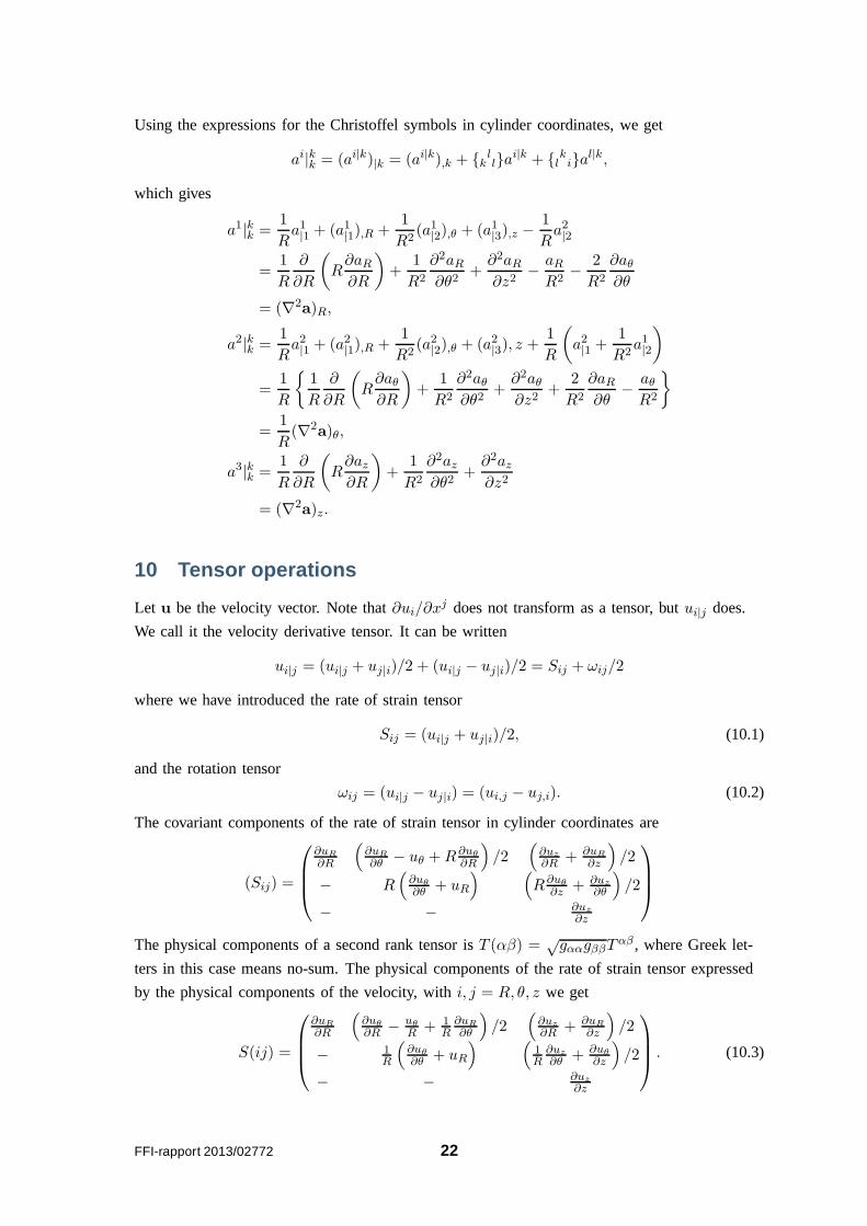
10 Tensor operations

Let u be the velocity vector. Note that∂ui/∂xj does not transform as a tensor, butui|j does.

We call it the velocity derivative tensor. It can be written

ui|j = (ui|j + uj|i)/2 + (ui|j − uj|i)/2 = Sij + ωij/2

where we have introduced the rate of strain tensor

Sij = (ui|j + uj|i)/2, (10.1)

and the rotation tensor

ωij = (ui|j − uj|i) = (ui,j − uj,i). (10.2)

The covariant components of the rate of strain tensor in cylinder coordinates are

(Sij) =

∂uR

∂R

(

∂uR

∂θ− uθ +R∂uθ

∂R

)

/2(

∂uz

∂R+ ∂uR

∂z

)

/2

− R(

∂uθ

∂θ+ uR

) (

R∂uθ

∂z+ ∂uz

∂θ

)

/2

− − ∂uz

∂z

The physical components of a second rank tensor isT (αβ) =√gααgββT

αβ , where Greek let-

ters in this case means no-sum. The physical components of the rate of strain tensor expressed

by the physical components of the velocity, withi, j = R, θ, z we get

S(ij) =

∂uR

∂R

(

∂uθ

∂R− uθ

R+ 1

R∂uR

∂θ

)

/2(

∂uz

∂R+ ∂uR

∂z

)

/2

− 1R

(

∂uθ

∂θ+ uR

) (

1R

∂uz

∂θ+ ∂uθ

∂z

)

/2

− − ∂uz

∂z

. (10.3)


Sometimes it can be of practical interest to express the components of a symmetric tensor in

Cartesian coordinatesyi, we denote itsij, derived from its componentsSij in generalized

coordinatesxi. We have

sij =∂xk

∂yi∂xl

∂yjSkl.

Using the covariant components of a symmetric tensorSij in cylinder coordinates, we get the

following Cartesian components

s11 = (cos2 θ)S11 − (sin(2θ)/R)S12 + (sin2 θ/R2)S22,

s12 = s21 = (sin(2θ)/2)S11 + (cos(2θ)/R)S12 − (sin(2θ)/2R2)S22,

s13 = s31 = (cos θ)S13 − (sin θ/R)S23,

s22 = (sin2 θ)S11 + (sin(2θ)/R)S12 + (cos2 θ/R2)S22,

s23 = s32 = (sin θ)S13 + (cos θ/R)S23,

s33 = S33.

These expressions may be useful when visualizing symmetrictensors where the components are

given in for example cylinder coordinates and the coordinate system used by the visualization

system is Cartesian.

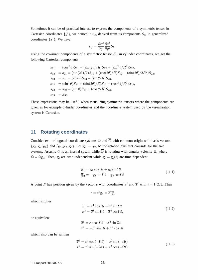
11 Rotating coordinates

Consider two orthogonal coordinate systemsO andO with common origin with basis vectors

g1,g2,g3 andg1,g2,g3. Let g3 = g3 be the rotation axis that coinside for the two

systems. AssumeO is an inertial sysem whileO is rotating with angular velocityΩ, where

Ω = Ωg3. Then,gi are time independent whilegi = gi(t) are time dependent.

g1 = g1 cos Ωt+ g2 sinΩt

g2 = −g1 sinΩt+ g2 cos Ωt(11.1)

A point P has position given by the vectorr with coordinatesxi andxi with i = 1, 2, 3. Then

r = xigi = xigi

which impliesx1 = x1 cos Ωt− x2 sinΩt

x2 = x1 sinΩt+ x2 cosΩt,(11.2)

or equivalentx1 = x1 cos Ωt+ x2 sinΩt

x2 = −x1 sinΩt+ x2 cos Ωt,

which also can be written

x1 = x1 cos (−Ωt)− x2 sin (−Ωt)

x2 = x1 sin (−Ωt) + x2 cos (−Ωt).(11.3)


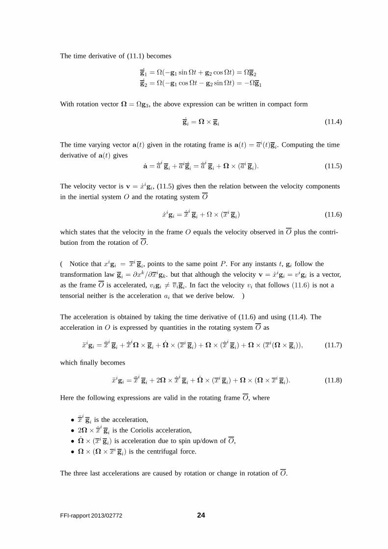
The time derivative of (11.1) becomes

g1 = Ω(−g1 sinΩt+ g2 cos Ωt) = Ωg2

g2 = Ω(−g1 cos Ωt− g2 sinΩt) = −Ωg1

With rotation vectorΩ = Ωg3, the above expression can be written in compact form

gi = Ω× gi (11.4)

The time varying vectora(t) given in the rotating frame isa(t) = ai(t)gi. Computing the time

derivative ofa(t) gives

a = aigi + aigi = a

igi +Ω× (ai gi). (11.5)

The velocity vector isv = xigi, (11.5) gives then the relation between the velocity components

in the inertial systemO and the rotating systemO

xigi = xigi +Ω× (xi gi) (11.6)

which states that the velocity in the frameO equals the velocity observed inO plus the contri-

bution from the rotation ofO.

( Notice thatxigi = xi gi, points to the same pointP . For any instantst, gi follow the

transformation lawgi = ∂xk/∂xigk. but that although the velocityv = xigi = vigi is a vector,

as the frameO is accelerated,vigi 6= vigi. In fact the velocityvi that follows (11.6) is not a

tensorial neither is the accelerationai that we derive below. )

The acceleration is obtained by taking the time derivative of (11.6) and using (11.4). The

acceleration inO is expressed by quantities in the rotating systemO as

xigi = xigi + x

iΩ× gi + Ω× (xi gi) +Ω× (x

igi) +Ω× (xi(Ω× gi)), (11.7)

which finally becomes

xigi = xigi + 2Ω× x

igi + Ω× (xi gi) +Ω× (Ω× xi gi). (11.8)

Here the following expressions are valid in the rotating frameO, where

• xigi is the acceleration,

• 2Ω× xigi is the Coriolis acceleration,

• Ω× (xi gi) is acceleration due to spin up/down ofO,

• Ω× (Ω× xi gi) is the centrifugal force.

The three last accelerations are caused by rotation or change in rotation ofO.


In rotating cylinder coordinateseR, eθ, ez with coordinates(R, θ, z), whereθ = θ − Ω, the

terms in (11.8) become

Ω× (Ω× xi gi) = Ω× (Ω× r) = −Ω2ReR (11.9)

Ω× (xi gi) = ΩReθ (11.10)

2Ω× vigi = 2Ω(vReθ − vθeR) (11.11)

12 Navier Stokes equations in cylinder coordinates

In coordinate free form, the compressible Navier Stokes equations including momentum and

mass conservation can be written

ρ

(

∂v

∂t+ (v · ∇)v

)

= −∇p+ µ∇2v (12.1)

and∂ρ

∂t+∇ · (ρv) = 0. (12.2)

wherev is velocity, p is the pressure,ρ the mass density andµ is the dynamic viscosity,ν =

µ/ρ is the kinematic viscosity. It is included in the definition of the Reynolds-numberRe =

UL/ν.

When deriving the Navier Stokes equations in cylinder coordinates, we start writing them

in generalized coordinatesxi. Let us express the momentum equation (12.1) selecting the

covariant basisgi. Note that it is equivalent to express the equations in thegi system.

Assuming that the coordinate system does not vary in time,∂gi/∂t = gi = 0, then

∂v

∂t=∂vi

∂tgi.

The advective term becomes

v · ∇v = vlgl · (vi|k)gigk = vl(vi|k)giδkl = vk(vi|k)gi.

For the pressure gradient, we have∇p = p|igi, and we have previously shown that

∇2v = (gklvi|l)|kgi = vi|kkgi.

Substituting these terms into (12.1), we obtain the Navier-Stokes equation for generalized

coordinates

ρ

(

∂vi

∂t+ vkvi|k

)

= −p|i + µvi|kk. (12.3)

The equation of continuity becomes

∂ρ

∂t+ (ρvi)|i = 0. (12.4)

The advection term and the pressure term can be written

vkvi|k = vk(vi,k + vσσik) and p|i = gikp,k.


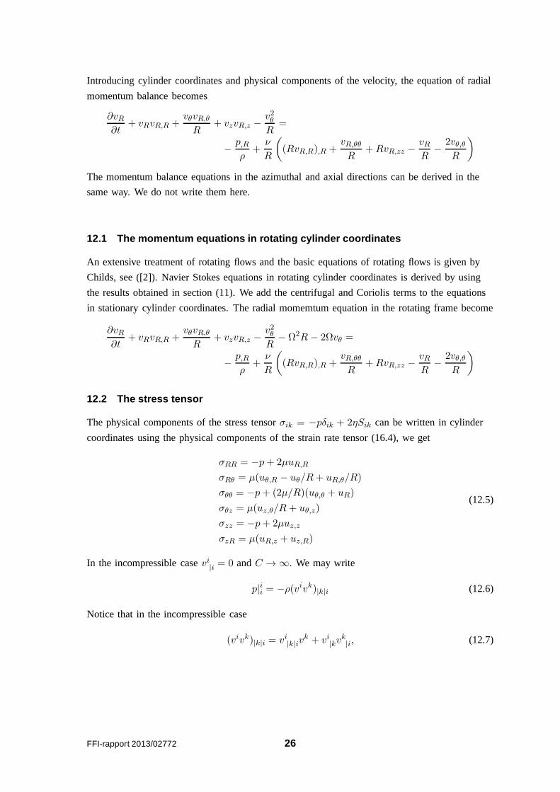
Introducing cylinder coordinates and physical componentsof the velocity, the equation of radial

momentum balance becomes

∂vR∂t

+ vRvR,R +vθvR,θ

R+ vzvR,z −

v2θR

=

− p,Rρ

+ν

R

(

(RvR,R),R +vR,θθ

R+RvR,zz −

vRR

− 2vθ,θR

)

The momentum balance equations in the azimuthal and axial directions can be derived in the

same way. We do not write them here.

12.1 The momentum equations in rotating cylinder coordinates

An extensive treatment of rotating flows and the basic equations of rotating flows is given by

Childs, see ([2]). Navier Stokes equations in rotating cylinder coordinates is derived by using

the results obtained in section (11). We add the centrifugaland Coriolis terms to the equations

in stationary cylinder coordinates. The radial momemtum equation in the rotating frame become

∂vR∂t

+ vRvR,R +vθvR,θ

R+ vzvR,z −

v2θR

− Ω2R− 2Ωvθ =

− p,Rρ

+ν

R

(

(RvR,R),R +vR,θθ

R+RvR,zz −

vRR

− 2vθ,θR

)

12.2 The stress tensor

The physical components of the stress tensorσik = −pδik + 2ηSik can be written in cylinder

coordinates using the physical components of the strain rate tensor (16.4), we get

σRR = −p+ 2µuR,R

σRθ = µ(uθ,R − uθ/R+ uR,θ/R)

σθθ = −p+ (2µ/R)(uθ,θ + uR)

σθz = µ(uz,θ/R + uθ,z)

σzz = −p+ 2µuz,z

σzR = µ(uR,z + uz,R)

(12.5)

In the incompressible casevi|i = 0 andC → ∞. We may write

p|ii = −ρ(vivk)|k|i (12.6)

Notice that in the incompressible case

(vivk)|k|i = vi|k|ivk + vi|kv

k|i, (12.7)


since generallyvi|k|i 6= vi|i|k = 0. In the incompressible case with Cartesian coordinates

differentiation commute and

∂2p

∂xi∂xi=− ∂vi

∂xj∂vj

∂xi=

1

4

(

∂vj

∂xi− ∂vi

∂xj

)(

∂vj

∂xi− ∂vi

∂xj

)

− 1

4

(

∂vj

∂xi+∂vi

∂xj

)(

∂vj

∂xi+∂vi

∂xj

)

=

ΩijΩij − SijSij ,

whereSij is the strain rate tensor andΩij = ωij/2 andωij is rotation tensor as defined in sec-

tion (10). This does not generally apply since the second covariant derivatives do not commute,

i.e. vi|k|i 6= vi|i|k in curved space.

We recognize(ΩijΩij−SijSij)/2 = Q > 0 as Hunt’s criteria to identify a vortex, see [4], where

rotation dominates over strain. TheQ criteria should be used with some care in the general

case since it is not clear thatQ as defined above is a tensorial quantity. Generally,2Q =

−ρ(vivk)|k|i should be used. This deserves some additional analysis since Sij = (∂vi/∂xj +

∂vj/∂xi)/2 is not a tensor. The criteria for identifying a vortex has also been discussed Jeong

and Hussain, see [6], using the second eigenvalue,λ2 < 0 criteria ofSijSij + ΩijΩij . As

proposed in [6], it is not clear thatλ2 is a tensorial quantity. It should be used with care in

non-Cartesian coordinate systems and deserves some additional analysis.

13 Lighthill’s equation in generalized coordinates

Lighthill’s equation can be derived from the Navier-Stokesequations, involving both thermal

and viscous dissipation, see (James Lighthill). Here we neglect effects of dissipation and start

with the Euler equations for compressible flows

ρ

(

∂v

∂t+ (v · ∇)v

)

= −∇p, ∂ρ

∂t+∇ · (ρv) = 0. (13.1)

By assuming that the motion is adiabatic, i.e isentropic flow, δp = C2δρ, wherep is the

pressure,C is the sound speed andρ is the density, one can show that the equations can be

written in an equivalent form where the left hand side has theform of a wave-equation. In

coordinate-free form, Lighthill’s equation can be written

1

C2

∂2p

∂t2−∇2p = ∇ · (∇ · (ρvv))

whereρvv is the momentum flux density tensor.

From the Euler equations (13.1) we have

0 =∂(ρvi)

∂t− ρ

∂vi

∂t− vi

∂ρ

∂t=∂(ρvi)

∂t+ (ρvkvi)|k + p|i.


Sincegij|k = 0, and lowering the index, we can writep|i = gikp|k = (pgik)|k and

∂(ρvi)

∂t+ (ρvivk + pgik)|k = 0.

Assuming isentropic conditions and constant speed of soundC, δp = C2δρ and we have

1

C2

∂2p

∂t2=∂2ρ

∂t2.

Taking the time derivative of the equation of continuity andthe divergence of the momentum

equation (13.1) we get∂2ρ

∂t2= −

∂(ρvi)|i

∂t= (ρvivk + pgik)|k|i

which can be written1

C2

∂2p

∂t2− p|ii = (ρvivk)|k|i. (13.2)

This is the component form of Lighthill’s equation in generalized coordinates.

14 Lighthill’s equation in cylinder coordinates

Now we want to express the right side of equation (13.2) in cylinder coordinates with the

physical velocity components(vR, vθ, vz) as arguments. The termp|ii is obtained in section (9),

so we skip it here. The double divergence is more complex. Letus take it in steps, first we

write

(ρvivk)|k|i = T ik|k|i =

( 1√g(√gT ik),k + T lklik

)

|i= ai|i.

The components of vectora are

ai = T ik|k = T ik

,k + T lklik+ T ilkkl.

The divergence ofai becomes

ai|i =1√g

(√gai

)

,i=a1

R+ a1,R + a2,θ + a3,z.

By substituting the expressionai = T ik|k into the above relation yields

T ik|k|i = ai|i =

1R

(

T 1k,k −RT 22 + 1

RT 11

)

+(

T 1k,k −RT 22 + 1

RT 11

)

,R

+(

T 2k,k +

1R(T 12 + T 21) + 1

RT 21

)

,θ

+(

T 3k,k +

1RT 31

)

,z.

SinceT ik is symmetric, this expression can be expanded and simplified

T ik|k|i = T 11

,RR + 2RT 11

,R + T 22,θθ − 2T 22 + T 33

,zz +4RT 12

,θ

+ 2RT 13

,z + 2T 12,Rθ + 2T 23

,θz + 2T 13,Rz −RT 22

,R.


Substituting the phyaical components of the velocity field,we have

(T ij) =

ρ(v1)2 ρv1v2 ρv1v3

− ρ(v2)2 ρv2v3

− − ρv3v3

=

ρv2R ρvRvθ/R ρvRvz

− ρv2θ/R2 ρvθvz/R

− − ρv2z

,

which implies

T ik|k|i = (ρv2R),RR + (ρv2θ/R

2),θθ + (ρv2z),zz +2R(ρv2R),R

+ 2R2 (ρvRvθ),θ +

2R(ρvRvz),z +

2R(ρvRvθ),Rθ +

2R(ρvθvz),θz

+2(ρvRvz),Rz − 1R(ρv2θ),R,

(14.1)

which is the right hand side of Lighthill’s equation in cylinder coordinates with the physical

components of the velocity field as arguments. Notice thatT ik|k|i is a scalar.

15 The RANS equations

A field quantityf is decomposed in an average quantityF and a fluctuating quantityf ′. We

write f = F + f ′. The averaging procedures are such that

F = f ⇒ (15.1)

f ′ = 0, (15.2)

fg = fg, (15.3)

fg′ = 0. (15.4)

For details, see ([13]) where the evolution equation for theReynolds stress is developed in

Cartesian coordinates. An extension to generalized coordinates follows below.

Assuming incompressibilityvi|i = 0, both v′i|i andV i|i = 0. Taking equation (12.3), substituting

the decomposition off and averaging, we get the averaged momentum equation

∂V i

∂t+ V kV i

|k = −1

ρP |i + νV i|kk −Rik

|k. (15.5)

The termsRik = v′iv′k represent the contravariant components of the Reynolds stress tensor.

Subtracting (15.5) from the equation forvi gives the following equation

∂v′i

∂t+ V kv′i|k + v′kV i

|k = −1

ρp′|i − (v′iv′k − v′iv′k)|k + νv′i|kk, (15.6)

which is the fluctuating momentum equation. From now, we write x for the fluctiating quanti-

ties instead ofx′. Taking thei component the fluctuating momentum equation and multiplying

with vj, the j component of the same equation and multiplying withvi summing and averag-


ing, we get the Reynolds stress evolution equation in generalized coordinates

∂(vivj )∂t

= −V k(vivj)|k convection

−(vjvkV i|k + vivkV j

|k) turbulent production

−(uiujuk)|k turbulent diffusion

−1ρ(giσ(pv)j

|σ+ gjσ(pv)i |σ) pressure diffusion

+1ρ(giσpvj|σ + gjσpvi|σ) pressure strain

+νgkσ(vivj)|kσ viscous diffusion

−νgkσ(vi|kvj|σ + vi|σv

j|k) viscous dissipation

(15.7)

Notice the existense of a termuiujuk which implies a closure problem. The terms above can

be written out in cylinder coordinates. Note thatvivj is a contravariant tensor.

We write the evolution equation for the this expression, theReynolds stress (15.7) as follws

∂Rij

∂t= Cij + T ij

p + T ijd + P ij

d + P ijs + V ij

diff + V ijdiss. (15.8)

This tensors physcal components can be calculated using expression (7.8). For exampleArθ =

rA12, Arz = A13, Aθθ = r2A22. Let us as calculate some of the terms in cylinder coordinates as

examples. The pressure diffusion tensor is

P ijd = −1

ρ(giσ(pv)j|σ + gjσ(pv)i|σ).

SubstitutingAi = (pv)i = pvi, we get using (6.6)

P ijd = −1

ρ

(

giσ(

∂Aj

∂xσ+Assjσ

)

+ gjσ(

∂Ai

∂xσ+Assiσ

))

.

Using this formula, the fact thatgij is diagonal and given by (7.4), that all Christoffel symbols

ijk are zero except122 = 221 = 1/r, 212 = −r and substituting for the physical vector

components ofAi, we get the following physical components for the pressure diffusion tensor

Pd(rr) = P 11d = −2

ρ

∂pvr∂r

= − 2

ρr

(

∂rpvr∂r

− pvr

)

,

Pd(rθ) = rP 12d = − 1

ρr

(

∂rpvθ∂r

+∂pvr∂θ

− 2pvθ

)

,

Pd(rz) = P 13d = −1

ρ

(

1

r

∂rpvz∂r

− 1

rpvz +

∂pvr∂z

)

,

Pd(θθ) = r2P 22d = − 2

ρr

(

∂pvθ∂θ

+ pvr

)

,

Pd(θz) = rP 23d = −1

ρ

(

1

r

∂pvz∂θ

+∂pvθ∂z

)

,

Pd(zz) = P 33d = −2

ρ

∂pvz∂z

.


16 Basic equations from the theory of elasticity

The treatment here is a generalization of the elasticity equations given in ([8]). Consider a point

P in a solid and assume the body is deformed such that pointP is displaced to another point

P ′. The displacement vector isup = r′p − rp. Consider another pointQ close toP. After

deformationQ is moved toQ′. The displacement vector forQ is uq = r′q − rq. The change in

the vector connectingP andQ due to displacement is

du = uq − up = (r′q − r′p)− (rq − rp),

which on component form is written

dui = dx′i − dxi.

The distance betweenP andQ before displacement isdl2 = dxidxi, and after displacement is

dl′2 = dx′idx′i. Due to continuity we write

dui =∂ui∂xj

dxj.

Then

dl′2 = dx2i + 2uijdxidxj ,

where

uij =1

2

(∂ui∂xj

+∂uj∂xi

)

+∂uk∂xi

∂uk∂xj

. (16.1)

Let us show thatuij is indeed a tensor we consider two coordinate systemsO andO. The line

elementsdl′ anddl are invariants. We write

(dl′)2 = dl2 + 2uijdxidxj ,

(dl′)2 = dl

2+ 2uijdx

idxj .

Sincedxi = (∂xi/∂xj)dxj and the line elements are invariants, we get

uij =∂xk

∂xi∂xl

∂xjukl,

showing thatuij are the covariant tensor components. The expression foruij given in (16.1) is

valid for Cartesian coordinates. Generally we may write thestrain tensor as

2uij = ((ui|j + uj|i) + uk|juk|i). (16.2)

If the deformation is small, we may omit the non-linear term in the above expression, then we

may write

uij =1

2

(∂ui∂xj

+∂uj∂xi

)

− uσiσj. (16.3)


Recall that the physical components of a vectorv(α) = vα√gαα and for a tensorT (α, β) =

Tαβ√gααgββ etc. . . Since a symmetric tensor is symmetric in all coordinate systems, we write

for i, j = 1, 2, 3

uij =

u1,1 (u1,2 + u2,1)/2− u2/r (u1,3 + u3,1)/2

− u2,2 + ru1 (u2,3 + u3,2)/2

− − u3,3

.

Using equation (7.7) for the physical components of a vectorwe calculate the physical compo-

nents of the strain tensor which has the same form as the strain rate tensor, see (10.3)

u(ij) =

∂ur

∂r12r

(

∂ur

∂θ+ r ∂uθ

∂r− uθ

)

12

(

∂ur

∂z+ ∂uz

∂r

)

− 1r

(

∂uθ

∂θ+ ur

)

12

(

∂uθ

∂z+ 1

r∂uz

∂θ

)

− − ∂uz

∂z

. (16.4)

The stress tensor and body forces.

The total force on a body is∫

FdV , whereF is force/volume. According to the divergence

theorem of integration, for the vector fielda∮

S

a · ds =∫

V

∇ · a dV.

This can be generalized to a tensor field, sayσ∮

S

σikdSk =

∫

V

∂σij∂xk

dV =

∫

V

FidV.

Hereσij is the stress tensor andFi is the i component of the force (force/volume) related to the

stress,

Fi =∂σik∂xk

.

This formula is valid in Cartesian coordinates. Generally we may write in coordinate free form

F = ∇ · σ.

As an example we can derive the co-variant components of the force,Fi. Then we may look

for expressions likeσ ki |k. We have

∇ · σ = gk · ∂σji g

igj

∂xk.

Carrying out the derivation in this expression gives

∇·σ = gk·∂σji

∂xkgigj+σ

ji g

k· ∂gi

∂xkgj+σ

ji g

k·gi ∂gj∂xk

= δkj∂σ j

i

∂xkgi−σ j

i δkj mi

kgm+σ ji δ

kmjmkgi,

where we have used (4.6,4.7). Cleaning up, we get

Fi = (∇ · σ)i = σ ki |k =

∂σ ki

∂xk− σ k

s isk+ σ si skk.


As an example of equivalence of the co and contravariant vectors, we can use the contravariant

components which are more convenient when calculating the physical components. We have

F i = σik |k =∂σik

∂xk+ σsksik+ σisskk,

which implies that

F (α) =√gαα

(∂σαk

∂xk+ σsksαk+ σαsskk

)

. (16.5)

Introducing physical components, we get

Fr =∂σrr∂r

+1

r

∂σrθ∂θ

+∂σrz∂z

+1

r

(

σrr − σθθ

)

, (16.6)

Fθ =∂σrθ

∂r+

1

r

∂σθθ∂θ

+∂σθz∂z

+2

rσrθ, (16.7)

Fz =∂σrz∂r

+1

r

∂σθz∂θ

+∂σzz∂z

+σrzr. (16.8)


References

[1] Rutherford Aris. Vectors, Tensors and the Basic Equations of Fluid Mechanics. Dover

Publications, Inc., 1989. ISBN 0-486-66110-5.

[2] Peter R. N. Childs.Rotating Flow. Elsvier, 2011. ISBN 978-0-12-382098-3.

[3] John Heinbockel. Introduction to Tensor Calculus and Continuum Mechanics. Trafford

Publishing, 2006. ISBN 9781553691334.

[4] J. C. R. Hunt, A. A. Wray, and P. Moin. Eddies, stream, and convergence zones in turbu-

lent flows. Technical report, Center for Turbulence Research Report CTR-S88, 1998. p.

193.

[5] Fridtjov Irgens. Kontinumsmekanikk. Tapir, 1984. ISBN: 8251900832.

[6] J. Jeong and F. Hussain. On the identification of a vortex.J. Fluid Mech, 285:69–94, 1995.

[7] E. Kreyszig. Differential Geometry. Dover Publications INC., New York, 1991. ISBN-

13:978-0-486-66721-8.

[8] L. D. Landau and E. Me. Lifshitz.Theory of elasticity. Elsvier, 1986. ISBN 0 7506 2633

X.

[9] Sir James Lighthill. On sound generated aerodynamically. I. general theory.Proceedings

of the royal society of London. A. Mathematical and PhysicalSciences, 211:564–587, 1952.

[10] Sir James Lighthill. On sound generated aerodynamically. II. turbulence as a source of

sound. Proceedings of the royal society of London. A. Mathematicaland Physical Sciences,

222:1–32, 1954.

[11] Sir James Lighthill.Waves in fluids. Cambridge Uiversity Press, 1978. ISBN: 0 512 21689

3.

[12] David Lovelock and Hanno Rund.Tensors, Differential Forms, and Variational Principles.

Dover Publications, Inc., New York, 1989. ISBN: 0-486-65840-6.

[13] W. C. Reynolds. Special course on modern theoretical and experimental approaches to

turbulence flow structure and modeling. Technical Report AGARD-REPORT-No.755,

AGARD, Advisory Group for Aerospace Research and Development, 1988.

[14] Karl Rottmann. Mathematische Formelsamlung. Hochschultaschenbucher. Bibliographis-

ches Institut AG, Mannheim, GmbH, Speyer, 1960.


tensor analysis applied to the equations of continuum ... · tensor analysis applied to the...

Documents