tensor modelling of mimo communication systems with
TRANSCRIPT

HAL Id: hal-01871380https://hal.archives-ouvertes.fr/hal-01871380
Submitted on 10 Sep 2018
HAL is a multi-disciplinary open accessarchive for the deposit and dissemination of sci-entific research documents, whether they are pub-lished or not. The documents may come fromteaching and research institutions in France orabroad, or from public or private research centers.
L’archive ouverte pluridisciplinaire HAL, estdestinée au dépôt et à la diffusion de documentsscientifiques de niveau recherche, publiés ou non,émanant des établissements d’enseignement et derecherche français ou étrangers, des laboratoirespublics ou privés.
Tensor modelling of MIMO communication systems withperformance analysis and Kronecker receivers
Michele Nazareth da Costa, Gérard Favier, J Romano
To cite this version:Michele Nazareth da Costa, Gérard Favier, J Romano. Tensor modelling of MIMO communicationsystems with performance analysis and Kronecker receivers. Signal Processing, Elsevier, 2018. hal-01871380

Tensor modelling of MIMO communication systemswith performance analysis and Kronecker receivers
Michele Nazareth da Costaa, Gerard Favierb, J.M.T. Romanoa
aDSPCom laboratory, University of Campinas, Campinas-SP, BrazilbI3S Laboratory, University of Nice Sophia Antipolis, CNRS, Sophia Antipolis, France
Abstract
The purpose of this paper is manifold. In a first part, we present a newalternating least squares (ALS)-based method for estimating the matrix factorsof a Kronecker product, the so-called Kronecker ALS (KALS) method. Fourother methods are also briefly described. In a second part, we consider the designof multiple-input multiple-output (MIMO) wireless communication systemsusing tensor modelling. Eight systems are presented in a unified way, andtheir theoretical performance is compared in terms of maximal diversity gain.Exploiting a Kronecker product of symbol and channel matrices, and applyingthe algorithms introduced in the first part, we propose three semi-blind andtwo supervised receivers, called Kronecker receivers, for jointly estimating thechannel and the transmitted symbols. Necessary identifiability conditions areestablished. Finally, extensive Monte Carlo simulation results are provided tocompare the performance of three tensor-based systems, on the one hand, andof the five proposed Kronecker receivers for the tensor space-time-frequency(TSTF) coding system, on the other hand.
Keywords: Channel estimation; Kronecker product; MIMO systems;semi-blind receivers; tensor coding; tensor modelling.
1. Introduction
Kronecker products, also known as tensor products, of matrices are currentlyused in many signal and image processing applications, like in compressivesensing with Kronecker dictionaries [1] and for image restoration [2]. They areuseful in system theory [3] and in numerical linear algebra to write and solvelinear matrix equations like Lyapunov and more generally Sylvester equations[4]. They also play an important role to simplify and implement fast transformalgorithms like fast Fourier, Walsh-Hadamard, and Haar transforms [5, 6].
Email addresses: [email protected] (Michele Nazareth da Costa),[email protected] (Gerard Favier), [email protected] (J.M.T. Romano)
Preprint submitted to Elsevier December 22, 2017

Recently, Kronecker and Khatri-Rao (column-wise Kronecker) products havebeen extensively employed in tensor-based system analysis and modelling,since such products naturally appear in matrix unfoldings of basic tensordecompositions, like the parallel factor (PARAFAC) [7] and Tucker [8] ones, andmore generally of constrained PARAFAC models [9]. Reviews of the history andapplications of the Kronecker product can be found in [3, 10, 5, 6, 11].
In the first part of the paper, we propose a new efficient computationalalgorithm based on the alternating least-squares (ALS) method for solving theKronecker product approximation problem, i.e. for determining two matrices Aand B of predetermined sizes, whose Kronecker product approximates a givenmatrix C in the sense of the minimization of the Frobenius norm ‖C−A⊗B‖F .We also briefly describe four other methods for solving this problem.
During the last decade, tensorial approaches have been widely developed toexploit multiple diversities in wireless communication systems. The principle ofdiversity techniques is to exploit several copies of the information symbols tobe recovered at the receiver. This symbol repetition can result from multipath(due to multiantennas at the transmitter and receiver), repeated transmissionof same symbols during several time-slots, and also from specific codings like,for instance, space-time (ST), space-frequency (SF) or space-time-frequency(STF) codings, which induce spatial multiplexing and temporal spreading.Tensor-based multiple-input multiple-output (MIMO) systems allow to improvelink reliability as well as to jointly and semi-blindly estimate the channel andthe transmitted symbols by means of deterministic receivers operating on datablocks. They have the advantage not to require a priori channel knowledgeand long training sequences for estimating the channel. Only very few pilotsymbols are needed to eliminate scaling ambiguities inherent to each particulartensor model. Moreover, tensor codings lead to natural tensor formulations oftransmitted and received signals, and consequently to tensor system modellings.Tensor-based communication systems can be classified according to:
• the type of system (code-division multiple access (CDMA), orthogonalfrequency division multiplexing (OFDM), CDMA-OFDM);
• the type of coding (ST, STF; matrices/tensors);
• the presence (in [12, 13, 14, 15, 16]) or not (in [17, 18, 19, 20, 21, 22]) ofresource allocation, and their type (matrices/tensors);
• the type of tensor model: PARAFAC [17, 18], block PARAFAC [19, 20],BTD (block term decomposition) [21], CONFAC (constrained PARAFAC)[12], PARAFAC-Tucker2 (PARATUCK2) [13], PARATUCK-(2,4) [14],generalized PARATUCK [15, 16], nested PARAFAC [22].
A brief history of tensor-based systems is now reviewed by beginning withthe fundamental work [17], which links direct-sequence CDMA (DS-CDMA)systems with a PARAFAC model. In [18], a space-time (ST) coding basedon a Khatri-Rao (KR) product, denoted KRST, was derived by combining
2

a linear precoding for spatial multiplexing with a linear post-coding fortemporal spreading. In [20], the idea of tensor coding was introduced forthe first time. A three dimensional tensor allows to combine space-timecoding and spatial multiplexing, hence the term space-time multiplexing (STM)coding. The third-order tensor containing the received signals satisfies a blockconstrained PARAFAC model, with two constraint matrices which depend onthe multiplexing parameters.
In [12], a generalized ST spreading scheme was proposed for DS-CDMAsystems, using a precoding tensor which allocates the users’ data streamsand spreading codes to transmit antennas, by means of three resourceallocation matrices. The resulting transmission structure led to a third-ordertensor model, called CONFAC, for the received signals. In [13], space-timespreading-multiplexing was proposed by combining a matrix precoding withstream- and antenna-to-slot matrix allocations. The third-order tensor ofreceived signals then satisfies a PARATUCK2 model. In [14], the system of [13]was extended by considering a third-order tensor space-time coding, denotedTST, in order to exploit an extra chip diversity. That leads to a fourth-orderPARATUCK-(2,4) model for the received signals tensor.
More recently, tensor approaches have been developed for OFDM, andOFDM-CDMA systems. In [22], a double Khatri-Rao STF coding, denotedDKRSTF, was proposed for OFDM systems. This coding constitutes anextension of the KRST coding [18], obtained by combining space-frequencypre-coding with time spreading. The received signals form a fourth-ordertensor satisfying a nested PARAFAC model. In [15], a spatial coding matrixis combined with two third-order interaction tensors which control a jointtime-frequency allocation of data streams and transmit antennas. In [16], thecase of OFDM-CDMA systems is considered. The tensor space-time-frequency(TSTF) coding system was developed with the double objective of increasingthe diversity gain by means of a fifth-order coding tensor, which allows to exploitfour diversities (space, time, chip, and frequency) at the receiver, and simplifyingthe resource allocation by using a fourth-order allocation tensor to controlthe assignment of data streams to transmit antennas in the time-frequencydomain. That leads to a generalized PARATUCK model for the fifth-ordertensor containing the received signals.
The main contributions of this paper are summarized as follows:
• A new algorithm, called Kronecker-based ALS and denoted KALS, isproposed for solving the Kronecker product approximation problem.
• Eight tensor-based MIMO systems are presented in a unified way, using ageneralized PARATUCK model [16].
• A comparative theoretical performance analysis is carried out for theconsidered tensor-based systems, and the maximal diversity gain is derivedunder the assumption of flat or frequency-selective fading channels. Thetransmission rate and the bandwidth of each system are also given.
3

• Five new receivers exploiting a Kronecker product of the channel andsymbol matrices are derived for jointly estimating these matrices, threebeing semi-blind and two supervised. A necessary identifiability conditionis established for each system.
• Extensive Monte Carlo simulation results are shown to compare theperformance of three tensor-based systems, with zero-forcing (ZF)receivers in the case of perfect channel knowledge, on the one hand, andwith the KALS receivers for joint semi-blind symbol/channel estimation,on the other hand. Then, the performance of the five proposed Kroneckerreceivers is compared for the TSTF system.
The rest of the paper is organized as follows. In Section 2, we presentthe KALS method for solving the Kronecker product approximation problem.Four other algorithms are also described. In Section 3, eight tensor-basedsystems are presented in a unified way using a generalized PARATUCK tensormodel. In Section 4, a comparative theoretical performance analysis is carriedout for these systems. Section 5 presents five new Kronecker receivers whichuse the Kronecker product approximation algorithms introduced in Section2. Simulation results are shown in Section 6 to illustrate and compare theperformance of the STF, TST, and TSTF systems, and also of the five proposedKronecker receivers for the TSTF system. Finally, Section 7 concludes the paperwith some perspectives for future work.
Notations and properties: Scalars, column vectors, matrices, andhigher-order tensors are written with lower-case, boldface lower-case , boldfaceupper-case, and calligraphic letters, i.e. (a, a, A, A), respectively. AT, AH,A∗, and A† stand for transpose, Hermitian transpose, complex conjugate, and
Moore-Penrose pseudo-inverse of A, respectively. e(N)n is the n-th canonical
basis vector of RN , IN is the identity matrix of order N , 1N is the N×1 all-onescolumn vector, and ‖·‖F is the Frobenius norm. The operator vec(·) forms acolumn vector by stacking the columns of its matrix argument, whereas diag(·)forms a diagonal matrix from its vector argument, and bdiag(A1, . . . ,AK) formsa block-diagonal matrix with K diagonal blocks. The inverse of the vectorizationoperator is denoted unvec, so that x = vec (X) ∈ CJI ←→ X = unvec (x) ∈ CI×J .By convention, the order of dimensions in a product IJK is linked to theorder of variation of the corresponding indices (i, j, k). For instance, givena third-order tensor X ∈ CI×J×K with entry xi,j,k, its tall mode-1 matrixunfolding XJK×I ∈ CJK×I corresponds to a combination of its modes (j,k)such that j varies more slowly than k, implying xi,j,k = [XJK×I ](j−1)K+k,i.The Hadamard, Kronecker, and Khatri-Rao products are denoted by , ⊗, and, respectively. Given A ∈ CI×J ,B ∈ CK×L,C ∈ CJ×M ,D ∈ CL×N , we have
(A⊗B) (C⊗D) = (A C)⊗ (B D) ∈ CIK×MN , (1)
A⊗B = (A IJ)⊗ (IK B) = (A⊗ IK) (IJ ⊗B) , (2)
A⊗B = (II A)⊗ (B IL) = (II ⊗B) (A⊗ IL) . (3)
4

Given two tensors A ∈ CI1×···×IN×JN+1×···×JN+P and B ∈CI1×···×IN×KN+1×···×KN+Q , of respective orders N + P and N + Q, we definethe Hadamard product of A with B, along their common modes (i1, · · · , iN ),as the tensor C = A
i1,··· ,iNB of order N + P +Q whose entries are given by
ci1,··· ,iN ,jN+1,··· ,jN+P ,kN+1,··· ,kN+Q= ai1,··· ,iN ,jN+1··· ,jN+P
bi1,··· ,iN ,kN+1,··· ,kN+Q.
A background with extended bibliography on tensor tools anddecompositions, and their applications, is presented in tutorial papers [23, 9, 24].Concerning the tensor-based systems considered in this paper, a detailedpresentation can be found in the references given in Table 1.
2. Kronecker Product Approximation Methods
In this Section, we first present a new ALS-based method for estimatingthe matrix factors of a Kronecker product, the so-called KALS method. Then,four other methods for solving this problem are briefly described. In Section 5,these methods will be employed to derive three semi-blind and two supervisedreceivers for seven tensor-based communication systems.
2.1. Kronecker Alternating Least Squares (KALS) method
Consider the Kronecker product of A ∈ CI×J and B ∈ CK×L
C = A⊗B ∈ CIK×JL
∆=
C(1,1) · · · C(1,J)
.... . .
...C(I,1) · · · C(I,J)
=
a1,1B · · · a1,JB...
. . ....
aI,1B · · · aI,JB
, (4)
where C(i,j) ∆= ai,jB ∈ CK×L satisfies the following equation
vec(C(i,j)
)= ai,j vec(B) ∈ CLK×1. (5)
The least-squares (LS) estimate of the coefficient ai,j is given by
ai,j =(vec(B))
Hvec(C(i,j)
)‖B‖2F
. (6)
Reorganize the entries of C in the Kronecker product D = B⊗A such as
D∆= B⊗A = Π(row) C Π(col) ∈ CKI×LJ , (7)
Π(row) and Π(col) denoting row and column permutation matrices defined as
Π(row) ∆=
K∑k=1
I∑i=1
e(K)k e
(I)T
i ⊗ e(I)i e
(K)T
k ∈ RKI×IK ,
Π(col) ∆=
J∑j=1
L∑l=1
e(J)j e
(L)T
l ⊗ e(L)l e
(J)T
j ∈ RJL×LJ . (8)
5
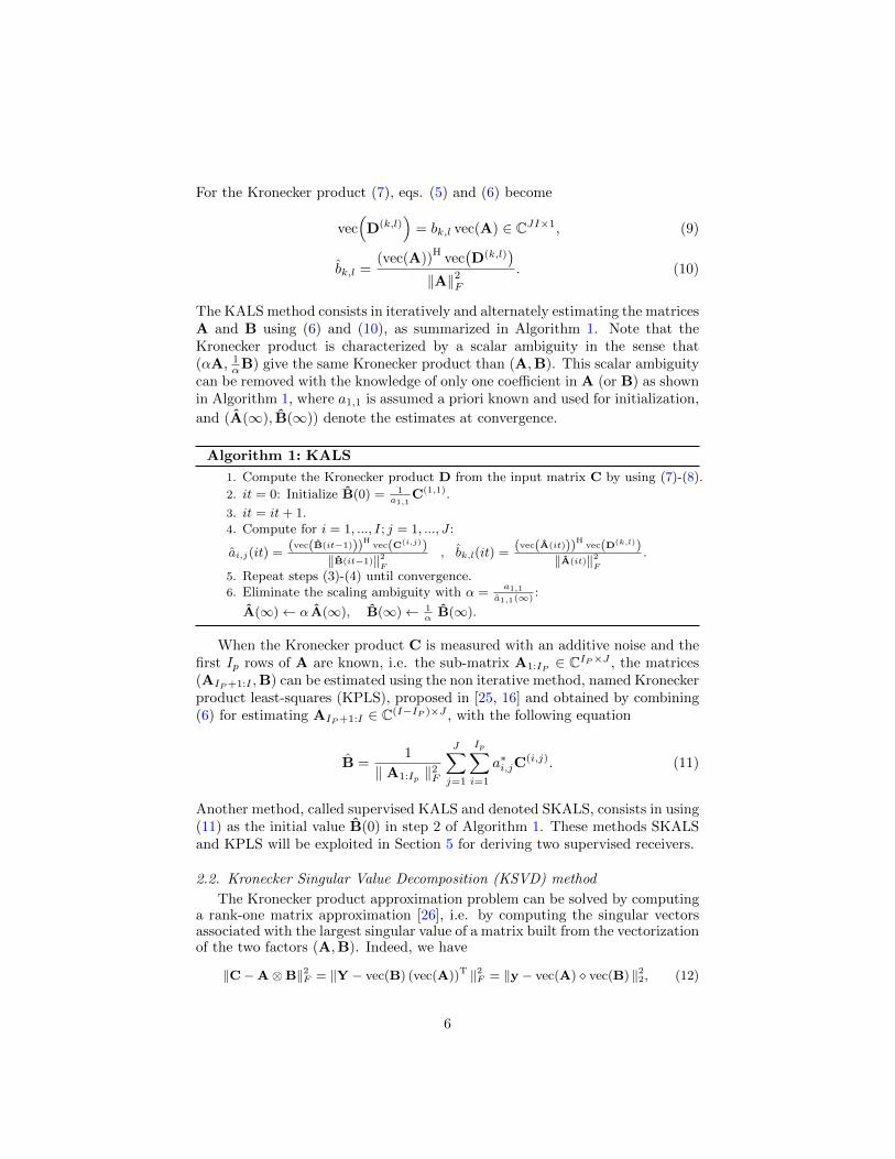
For the Kronecker product (7), eqs. (5) and (6) become
vec(D(k,l)
)= bk,l vec(A) ∈ CJI×1, (9)
bk,l =(vec(A))
Hvec(D(k,l)
)‖A‖2F
. (10)
The KALS method consists in iteratively and alternately estimating the matricesA and B using (6) and (10), as summarized in Algorithm 1. Note that theKronecker product is characterized by a scalar ambiguity in the sense that(αA, 1
αB) give the same Kronecker product than (A,B). This scalar ambiguitycan be removed with the knowledge of only one coefficient in A (or B) as shownin Algorithm 1, where a1,1 is assumed a priori known and used for initialization,
and (A(∞), B(∞)) denote the estimates at convergence.
Algorithm 1: KALS
1. Compute the Kronecker product D from the input matrix C by using (7)-(8).
2. it = 0: Initialize B(0) = 1a1,1
C(1,1).
3. it = it+ 1.4. Compute for i = 1, ..., I; j = 1, ..., J :
ai,j(it) =(vec(B(it−1)))H vec(C(i,j))
‖B(it−1)‖2F
, bk,l(it) =(vec(A(it)))H vec(D(k,l))
‖A(it)‖2F
.
5. Repeat steps (3)-(4) until convergence.6. Eliminate the scaling ambiguity with α =
a1,1a1,1(∞)
:
A(∞)← α A(∞), B(∞)← 1α
B(∞).
When the Kronecker product C is measured with an additive noise and thefirst Ip rows of A are known, i.e. the sub-matrix A1:IP ∈ CIP×J , the matrices(AIP+1:I ,B) can be estimated using the non iterative method, named Kroneckerproduct least-squares (KPLS), proposed in [25, 16] and obtained by combining(6) for estimating AIP+1:I ∈ C(I−IP )×J , with the following equation
B =1
‖ A1:Ip ‖2F
J∑j=1
Ip∑i=1
a∗i,jC(i,j). (11)
Another method, called supervised KALS and denoted SKALS, consists in using(11) as the initial value B(0) in step 2 of Algorithm 1. These methods SKALSand KPLS will be exploited in Section 5 for deriving two supervised receivers.
2.2. Kronecker Singular Value Decomposition (KSVD) method
The Kronecker product approximation problem can be solved by computinga rank-one matrix approximation [26], i.e. by computing the singular vectorsassociated with the largest singular value of a matrix built from the vectorizationof the two factors (A,B). Indeed, we have
‖C−A⊗B‖2F = ‖Y − vec(B) (vec(A))T ‖2F = ‖y − vec(A) vec(B) ‖22, (12)
6

where Y ∈ CLK×JI and y = vec(Y) ∈ CJILK×1 can be obtained by permutingthe elements of vec(C) ∈ CJLIK×1 as follows
y = vec(Y) = Π vec(C) ,
Π = IJ ⊗
(I∑i=1
L∑l=1
e(I)i e
(L)T
l ⊗ e(L)l e
(I)T
i
)⊗ IK ∈ RJILK×JLIK . (13)
Considering the rank-one approximation Y ≈ σ1uvH, where u and v are theleft and right singular vectors associated with the largest singular value σ1, onededuces the following estimates A = α
√σ1 unvec(v∗), B = 1/α
√σ1 unvec(u),
where the scalar α is calculated as in Algorithm 1. The power method [27] canbe applied for computing this rank-one approximation of Y. At each iteration,the right and left singular vectors are calculated as follows
v(it) =YH u(it− 1)
‖YH u(it− 1)‖2, σ1(it) = ‖Y v(it)‖2 , u(it) =
Y v(it)
σ1(it). (14)
The KSVD method is summarized in Algorithm 2.
Algorithm 2: KSVD
1. it = 0: Initialize u(0) = vec(B(0)
)= 1
a1,1vec(C(1,1)).
2. Compute the matrix Y = unvec(Π vec(C)) with Π defined in (13).3. it = it+ 1.4. Compute the rank-one approximation of Y ≈ σ1uvH using (14).5. Repeat steps (3)-(4) until convergence.6. Compute the estimates of A and B, with α =
a1,1a1,1(∞)
:
A = α√σ1(∞) unvec(v∗(∞)), B = 1
α
√σ1(∞) unvec(u(∞)).
2.3. Kronecker Alternating Least Mean Squares (KALMS) method
In [28], the identities (2)-(3) are exploited to iteratively estimate the factors(A,B) by applying a Kronecker-based alternating least mean squares (KALMS)algorithm to the input-output relationship y(it) = C x(it) + e(it) ∈ CIK×1,which defines a MIMO system from the Kronecker product C = A ⊗ B,with x(it) ∈ CJL×1 randomly generated. The signal e(it) representing bothmeasurement noise and modelling error, can be written in the following forms
e(it) = y(it)− (A⊗B) x(it)
= y(it)− (A⊗ IK) (IJ ⊗B) x(it) (15)
= y(it)− (II ⊗B) (A⊗ IL) x(it). (16)
The factors (A,B) are estimated by minimizing the LS cost function ‖e(it)‖22.This nonlinear optimization problem is replaced by the alternating minimization
7

of two quadratic cost functions obtained by fixing one of the factors to itsprevious estimated value in (15)-(16), i.e.
zA(it)∆=(IJ ⊗ B(it− 1)
)x(it) ∈ CJK×1
eA(it)∆= y(it)− (A⊗ IK) zA(it)
A(it) = minA
E[‖eA(it)‖22
] ,
zB(it)
∆=(A(it)⊗ IL
)x(it) ∈ CIL×1
eB(it)∆= y(it)− (II ⊗B) zB(it)
B(it) = minB
E[‖eB(it)‖22
] .
At each iteration, the LMS algorithm is used to update alternately theestimate of A and B. That results inK and I estimates of A and B, respectively,due to the presence of the Kronecker products A(it)⊗IK and II⊗B(it). Takingthe mean value of these estimates gives the Algorithm 3.
Algorithm 3: KALMS
1. Set γA and γB.
2. it = 0: Initialize B(0) = 1a1,1
C(1,1) and randomly initialize A(0).
3. it = it+ 1.4. Randomly generate the input signal x(it) and compute y(it) = C x(it).
5. Update of the estimate A(it):
zA(it)∆=(IJ ⊗ B(it− 1)
)x(it), ZA(it)
∆=(
unvec(zA(it)
) )T ∈ CJ×K ,
µA(it)∆= γA/
∥∥∥zA(it)∥∥∥22,
eA(it)∆= y(it)−
(A(it− 1)⊗ IK
)zA(it), EA(it)
∆=(
unvec(eA(it)
) )T ∈ CI×K ,
A(it) = A(it− 1) + µA(it)K
EA(it)(ZA(it)
)H.
6. Update of the estimate B(it):
zB(it)∆=(A(it)⊗ IL
)x(it), ZB(it)
∆= unvec
(zB(it)
)∈ CL×I ,
µB(it)∆= γB/
∥∥∥zB(it)∥∥∥22,
eB(it)∆= y(it)−
(II ⊗ B(it− 1)
)zB(it), EB(it)
∆= unvec
(eB(it)
)∈ CK×I ,
B(it) = B(it− 1) + µB(it)I
EB(it)(ZB(it)
)H.
7. Repeat steps (3)-(6) until convergence.8. Eliminate the scaling ambiguity with α =
a1,1a1,1(∞)
:
A(∞)← α A(∞), B(∞)← 1α
, B(∞).
3. Tensor modelling of MIMO communication systems
We first show that the TSTF coding structure, recently proposed in [16]for MIMO OFDM-CDMA systems, allows to deduce seven other tensor-basedsystems as particular cases.
Consider a MIMO system with M transmit and K receive antennas. Thetransmission is decomposed into P time blocks of N symbol periods, each onebeing composed of J chips. During each time block p, the transceiver uses Fsubcarriers to send R data streams containing N information symbols each,which form the symbol matrix S ∈ CN×R with entries sn,r, n= 1, ..., N ; r=1, ..., R. The transmission system is characterized by two tensors: a fifth-order
8

coding tensorW ∈ CM×R×F×P×J and a fourth-order resource allocation tensorC ∈ RM×R×F×P composed uniquely of 1’s and 0’s, cm,r,f,p=1 meaning that thedata stream r is transmitted using the transmit antenna m and the subcarrierf , during the time-block p. At the symbol period n of block p, the transceivertransmits a linear combination of R coded signals according to the equation
um,n,f,p,j =
R∑r=1
wm,r,f,p,j sn,r cm,r,f,p, (17)
where the coefficient cm,r,f,p of the allocation tensor C fixes the space-frequencyresource (m, f) used to send the symbol sn,r during the time block p. So, theallocation tensor controls the space-time-frequency spreading-mutiplexing. Eq.(17) shows that the multiplication by the coding tensor W allows to replicateeach symbol sn,r four times, in the space (m), frequency (f), time (p), andchip (j) dimensions. The high-order of the coding tensor is at the origin of aperformance improvement over other systems such as the ST, STF, and TSTones. This result will be theoretically established in the next section by acomparative analysis of the diversity gains.
The frequency-selective fading channel coefficients hk,m,f between each pair(m, k) of transmit and receive antennas, at frequency f , are assumed constantduring P time-blocks, independent, and circularly symmetric complex Gaussianvariables, with zero-mean and unit variance. They form a third-order tensorH ∈ CK×M×F . In the noiseless case, the received signals define a fifth-ordertensor X ∈ CK×N×F×P×J defined as
xk,n,f,p,j =
M∑m=1
hk,m,f um,n,f,p,j =
M∑m=1
R∑r=1
gm,r,f,p,j hk,m,f sn,r, (18)
gm,r,f,p,j = wm,r,f,p,j cm,r,f,p.
The core tensor G ∈ CM×R×F×P×J can be interpreted as the Hadamard productof the coding tensor with the allocation tensor, along their common modes(m, r, f, p), i.e. G =W
m,r,f,pC.
The received signal xk,n,f,p,j satisfies the generalized PARATUCK-(2,5)model introduced in [16], and defined as follows
xi1,i2,i3,i4,i5 =
R1∑r1=1
R2∑r2=1
gr1,r2,i3,i4,i5 a(1)i1,r1,i3
a(2)i2,r2
, (19)
gr1,r2,i3,i4,i5 = wr1,r2,i3,i4,i5 cr1,r2,i3,i4 .
Comparing (18) with (19), we deduce the following correspondences(I1, I2, I3, I4, I5, R1, R2,A(1),A(2)
)↔ (K,N,F, P, J,M,R,H,S) . (20)
9

Particular cases
In Tables 1 and 2, we present in a unified way eight tensor-based MIMOsystems which can be deduced as particular cases of the TSTF system. InTable 1, the core tensor G and the received signal tensor X are given for eachsystem, while Table 2 contains the design parameters for each system rewrittenas a generalized PARATUCK-(2,5) model (19).
Table 1: Presentation of eight tensor-based systems.
Systems Core tensors Received signals
TSTF [16] gm,r,f,p,j = wm,r,f,p,j cm,r,f,p xk,n,f,p,j =M∑m=1
R∑r=1
gm,r,f,p,j hk,m,f sn,r
STF [15] gm,r,f,p = wm,r c(H)m,f,p c
(S)r,f,p xk,n,f,p =
M∑m=1
R∑r=1
gm,r,f,p hk,m,f sn,r
TST [14] gm,r,p,j = wm,r,j c(H)m,p c
(S)r,p xk,n,p,j =
M∑m=1
R∑r=1
gm,r,p,j hk,m sn,r
ST [13] gm,r,p = wm,r c(H)m,p c
(S)r,p xk,n,p =
M∑m=1
R∑r=1
gm,r,p hk,m sn,r
STM [20] gm,r,p = wm,r,p xk,n,p =M∑m=1
R∑r=1
gm,r,p hk,m sn,r
DKRSTF [22] gm,r,f,p = wm,r,f,p = θm,r ωf,r ψp,m xk,n,f,p =M∑m=1
M∑r=1
gm,r,f,p hk,m sn,r
KRST [18] gm,r,p = wm,r,p = θm,r ψp,m xk,n,p =M∑m=1
M∑r=1
gm,r,p hk,m sn,r
DS-CDMA [17] gj,m = wj,m xk,n,j =M∑m=1
gj,m hk,m sn,m
Table 2: Design parameters for the associated generalized PARATUCK-(2,5) model.
SystemsDesign parameters
I1 I2 I3 I4 I5 R1 R2 A(1) A(2) C W
TSTF [16] K N F P J M R H S C WSTF [15] K N F P - M R H S C(H), C(S) W
TST [14] K N P J - M R H S C(H),C(S) WST [13] K N P - - M R H S C(H),C(S) W
STM [20] K N P - - M R H S - WDKRSTF [22] K N F P - M M H S - W
KRST [18] K N P - - M M H S - WDS-CDMA [17] K N J - - M - H S - W
From these two tables, we can draw the following conclusions:
• Two main features distinguish TSTF from the other systems. The firstone concerns the use of a fifth-order tensor (W) for space-time-frequencycoding, instead of a fourth-order (or third-order) coding tensor forDKRSTF (or TST, STM, and KRST), respectively, or of a codingmatrix in the case of STF, ST, and DS-CDMA. The five dimensionalcoding tensor allows to increase the diversity gain, which facilitatesperformance/complexity tradeoffs in all the signaling dimensions. The
10

second one is linked to the use of a fourth-order allocation tensor (C),while the other systems use either two third-order tensors as with STF,or two matrices as with ST and TST. The use of a single fourth-orderallocation tensor provides higher flexibility for allocations.
• The TSTF system can be viewed as an OFDM extension of the TSTsystem with a multicarrier transmission, and a CDMA extension of theSTF system. It can also be viewed as an extension of the DKRSTF systemwhich is itself an extension of the KRST one. Indeed, for KRST coding,the coded signals define a third-order tensor U ∈ CM×N×P such as
um,n,p =
M∑r=1
θm,r ψp,m sn,r , UNP×M = SΘT Ψ, (21)
while for the DKRSTF coding, the tensor U ∈ CM×N×F×P is such as
um,n,f,p =
M∑r=1
θm,r ωf,r ψp,m sn,r , UNFP×M = (S Ω)ΘT Ψ. (22)
This matrix unfolding highlights the double Khatri-Rao STF coding,the first one corresponding to a space-frequency pre-coding, whereas thesecond one corresponds to a time post-coding.These Eqs. (21) and (22) are to be compared with (17), showing that theKRST and DKRSTF systems exploit third- and fourth-order coded signalstensors, respectively, when TSTF uses a fifth-order coding tensor. Notealso the restrictive assumption for DKRSTF which requires the channelH ∈ CK×M constant across the F subcarriers, while it is a third-ordertensor H ∈ CK×M×F depending on the F frequencies, in the case ofTSTF. Another restriction shared by DKRSTF and KRST concerns thenumber of transmitted data streams which must be equal to the numberof transmit antennas (R=M), which is not the case of the other systems.
• In their original formulation, the received signals tensors satisfy thefollowing tensor models: PARAFAC, block PARAFAC, nested PARAFAC,PARATUCK2, PARATUCK-(2,4), and generalized PARATUCK-(2,5) forthe (DS-CDMA, KRST), STM, DKRSTF, ST, TST, and (STF,TSTF)systems, respectively. Moreover, all the systems use iterative ALS-basedreceivers for jointly estimating the channel and the information symbols.
• The rewriting of the received signals tensors presented in Table 1, by meansof generalized PARATUCK models, will allow us to derive closed-formreceivers for all systems, in Section 5. These receivers are based on thesame Kronecker product between the symbol matrix (S) and the channelmatrix (H or HK×FM ), as summarized in Table 4.
Now, we recall two matrix unfoldings of the tensor X which will be used inSections 4 and 5 for deriving the diversity gain and the Kronecker receivers of
11

the TSTF system (See eqs. (15) and (19) in [16])
XN×JPFK = S GR×JPFM
(IJP⊗ bdiag
(HT··1, · · · ,HT
··F)), (23)
XNK×FPJ = (S⊗HK×FM ) GRFM×FPJ , (24)
with
GR×JPFM∆=[
GT··1,1,1 · · · GT
··F,P,J
]∈ CR×JPFM ,
GRFM×FPJ∆=
bdiag
vec(GT
1,1,1··)T
...
vec(GTM,1,1··
)T , · · · ,
vec(GT
1,1,F ··)T
˜...
vec(GTM,1,F ··
)T
...
bdiag
vec(GT
1,R,1··)T
...
vec(GTM,R,1··
)T , · · · ,
vec(GT
1,R,F ··)T
...
vec(GTM,R,F ··
)T
,
G··f,p,j = W··f,p,j m,r
C··f,p, Gm,r,f ·· = Wm,r,f ·· p
cm,r,f · (25)
where HK×FM is a matrix unfolding of the channel tensor H ∈ CK×M×F , andH··f ∈ CK×M is a matrix slice obtained by fixing the index f of H, whichcorresponds to the channel matrix associated with the subcarrier f . Similarly,G··f,p,j ,W··f,p,j ,C··f,p ∈ CM×R denote matrix slices of G,W, C, obtainedby fixing (f, p, j), whereas Gm,r,f ··,Wm,r,f ·· ∈ CP×J and cm,r,f · ∈ CP×1
denote matrix slices of G,W, and a vector slice of C, respectively, obtainedby fixing (m, r, f).
4. Performance analysis
We first analyze the theoretical performance of the TSTF system by derivingits diversity gain. For this system, it is possible to jointly estimate theinformation symbols and the channel, without decoding of a codeword asrequired by standard ST and STF codings. The performance analysis is based onthe pairwise error probability (PEP) of the maximum likelihood (ML) estimatorof the symbol matrix S. The diversity gain d is defined as the negative of theasymptotic slope of the plot PEP(ρ) on a log-log scale, where ρ denotes thereceived signal-to-noise ratio (SNR). We assume that the receiver has perfectknowledge of the channel, allocation, and coding tensors.
Let us recall that the average PEP between S and S, conditioned on channelrealizations, is given by [29, 30]
P(S→ S
)= Q
(1
2√N0/2
‖X − X‖F
)=
1
π
∫ π2
0
exp
(− ‖X − X‖
2F
4N0 sin2(β)
)dβ, (26)
12

where N0/2 is the noise variance per (real and imaginary) dimension and Q(·)is the complementary cumulative distribution function of a Gaussian variable,written using the Craig’s formula [30]. Fixing the indices (f, p, j) in (18) gives
X··f,p,j = H··f U··f,p,j = H··f G··f,p,j ST ∈ CK×N . (27)
Defining the estimation error of codeword matrix slices
E(f,p,j) ∆= U··f,p,j − U··f,p,j = G··f,p,j
(S− S
)T
∈ CM×N (28)
and using (27), we have
‖X − X‖2F =
F∑f=1
P∑p=1
J∑j=1
‖X··f,p,j − X··f,p,j‖2F =
F∑f=1
P∑p=1
J∑j=1
‖H··f E(f,p,j)‖2F
=
F∑f=1
P∑p=1
J∑j=1
tr(H··f A(f,p,j) HH
··f
)=
F∑f=1
P∑p=1
J∑j=1
y(f,p,j), (29)
where A(f,p,j) ∆= E(f,p,j)
(E(f,p,j)
)His Hermitian nonnegative definite, and
y(f,p,j) ∆= tr
(H··f A(f,p,j) HH
··f
)=[vec(HT··f) ]T(
IK ⊗A(f,p,j))
vec(HH··f).
The channel coefficients hk,m,f being assumed i.i.d and drawn from a circularsymmetric complex Gaussian distribution with zero-mean and unit variance,application of the theorem E.1 on page 418 of [31] leads to
P(S→ S
)=
1
π
∫ π2
0
F∏f=1
P∏p=1
J∏j=1
[det
(IM +
1
4N0 sin2(β)A(f,p,j)
)]−Kdβ.
In order to simplify the calculation of the integral, we use the Chernoff bound[30, 31], obtained by taking sin2(β) = 1, which gives the following upper bound
P(S→ S
)≤
F∏f=1
P∏p=1
J∏j=1
[det
(IM +
1
4N0A(f,p,j)
)]−K. (30)
Since det(I + αA) =∏rank(A)i=1 (1 + αλi(A)), where λi(A) denotes an
eigenvalue of A, we can rewrite (30) as
P(S→ S
)≤
F∏f=1
P∏p=1
J∏j=1
r(f,p,j)∏i=1
(1 +
1
4N0λ
(f,p,j)i
)−K, (31)
13

where λ(f,p,j)i denotes the non-zero eigenvalues of A(f,p,j), and r(f,p,j) ∆
=rank
(A(f,p,j)
)= rank
(E(f,p,j)
). At high SNR, i.e. for small values of N0, the
upper bound on the PEP becomes
P(S→ S
)≤
F∏f=1
P∏p=1
J∏j=1
r(f,p,f)∏i=1
(λ
(f,p,j)i
)−K ( 1
4N0
)−K ∑f,p,j
r(f,p,j)
, (32)
which gives the following diversity gain
dTSTF = K
F∑f=1
P∑p=1
J∑j=1
r(f,p,j). (33)
Assuming S is full column rank, which implies N ≥ R (or N ≥M for KRSTand DKRSTF), and applying the property rank(AB) ≤ min(rank(A) rank(B)),we deduce from (28) that r(f,p,j) = rank
(E(f,p,j)
)≤ min(M,R), ∀f, p, j. It is
interesting to note from (25) and (28) that the maximum rank of G··f,p,j , andconsequently of E(f,p,j), depends on the allocation tensor C.
Define α(f,p) and β(f,p) as the numbers of transmit antennas used and of datastreams transmitted with the subcarrier f , during the time block p. Noting thatC··f,p, and consequently G··f,p,j for all j, have M−α(f,p) zero rows and R−β(f,p)
zero columns, we deduce that r(f,p,j) = rank(G··f,p,j) ≤ min(α(f,p), β(f,p)
)for
all j. So, a maximal diversity gain is given by:
dTSTFmax = KJ
F∑f=1
P∑p=1
min(α(f,p), β(f,p)
). (34)
The expression (34) can be upper bounded by dTSTFmax =KFPJ min(M,R) when
choosing α(f,p) = M , β(f,p) = R, for all (f, p), which includes a full allocationstrategy corresponding to the case where all data streams are transmitted by allantennas, using all subcarriers, during each time block p. Therefore, the TSTFcoding provides higher diversity gain than standard matrix ST coding schemesthat ensure a maximal diversity gain equal to KM . Moreover, for fixed numbers(K and M) of receive and transmit antennas, the maximal diversity gain dTSTF
max
can be increased by increasing the design parameters F , P , and J .The diversity gain and the maximal diversity gain for the other systems
can be easily deduced from (33)-(34), using the unified presentation in Table1, which leads to the results presented in Table 3, where α(p) and β(p) (α(f,p)
and β(f,p)) denote the number of non-zero elements of c(H)·p and c
(S)·p (c
(H)·f,p and
c(S)·f,p), for TST and ST (STF, respectively).
Remark that, in the case of DKRSTF, KRST and DS-CDMA, the maximaldiversity gain is proportional to M since the number of data streams is equalto the number of transmit antennas (R=M) for these systems.
Note also that for a full allocation strategy (α(f,p) =α(p) =M , β(f,p) =β(p) =R, for all p ∈ 1, ..., P and f ∈ 1, ..., F), i.e. in choosing all the entries of
14

the allocation matrix/tensor equal to 1, the maximal diversity gains are upperbounded by dSTF
max = KFP min(M,R), dTSTmax = KJP min(M,R), and dST
max =KP min(M,R), showing that the TSTF coding provides the highest diversitygain. Comparing TST and STF, with F = J , we conclude that dSTF
max = dTSTmax .
However, when all the subcarriers are not used, we have dSTF<dTST, explainingwhy the TST system offers better performance than STF when full frequencyallocation is not considered.
Table 3: Diversity gains
Systems Diversity gains Maximal diversity gains τ
TSTF [16]K
F∑f=1
P∑p=1
J∑j=1
rank
(G··f,p,j
(S− S
)T)
KJF∑f=1
P∑p=1
min(α(f,p), β(f,p)
)RFP
G··f,p,j = W··f,p,j m,r
C··f,p
STF [15]K
F∑f=1
P∑p=1
rank
(G··f,p
(S− S
)T)
KF∑f=1
P∑p=1
min(α(f,p), β(f,p)
)RFP
G··f,p = diag(c(H)·f,p
)W diag
(c(S)·f,p
)TST [14]
KJ∑j=1
P∑p=1
rank
(G··p,j
(S− S
)T)
KJP∑p=1
min(α(p), β(p)
)RP
G··p,j = diag(c(H)·p
)W··j diag
(c(S)·p
)ST [13]
KP∑p=1
rank
(G··p
(S− S
)T)
KP∑p=1
min(α(p), β(p)
)RP
G··p = diag(c(H)·p
)W diag
(c(S)·p
)STM [20]
KP∑p=1
rank
(G··p
(S− S
)T)
KP min(M,R) RP
G··p = W··p
DKRSTF [22]K
F∑f=1
P∑p=1
rank
(G··f,p
(S− S
)T)
KFPM MFP
G··f,p = diag(ψp·)Θ diag(ωf·)
KRST [18] KP∑p=1
rank
(G··p
(S− S
)T)
KPM MP
G··p = diag(ψp·)Θ
DS-CDMA [17] KJ∑j=1
rank
(diag(gj·)
(S− S
)T)
KJM M
The transmission rate, in bits per channel use, is given by Rb = τ log2(µ),where µ denotes the cardinality of the symbol alphabet set, i.e. the numberof constellation points, and the ratio τ is given in Table 3 for all systems.As expected, for STF and TSTF, an increase of P and/or F decreases thetransmission rate, while an increase of R increases it. For TSTF, TST, STFand ST, the bandwidth is given by, FJ
T , JT , F
T , and 1T , respectively, where T is
the symbol period.
5. Kronecker semi-blind receivers
Assuming a perfect knowledge of the coding and allocation matrices/tensorsat the receiver, we propose five receivers for all the systems presented in
15

Section 3. These receivers based on a Kronecker product approximation use thealgorithms described in Section 2. So, they are called KALS, SKALS, KPLS,KSVD, and KALMS. Note that SKALS and KPLS correspond to supervisedreceivers since they use a pilot sequence constituted by the first Np rows of S.In the sequel, we detail the Kronecker receivers for the TSTF system, the matrixunfolding (24) being exploited to jointly estimate the symbol matrix S and theunfolding HK×FM of the channel tensor. Similar Kronecker receivers can beeasily derived for the other systems using the matrix unfoldings given in Table4. Note that, for TST, ST, STM, KRST, and DKRSTF, the unfolding HK×FMis replaced by the channel matrix H.
Table 4: Matrix unfoldings of the received signals tensor X .
Systems Unfoldings with a Kronecker ProductIdentifiability
conditions
TSTFXNK×FPJ = (S⊗HK×FM ) GRFM×FPJ PJ ≥MRGRFM×FPJ ∈ CRFM×FPJ defined in (25)
STF†XNK×FP = (S⊗HK×FM ) GRFM×FP
P ≥MRGRFM×FP = Π bdiag(G(1), . . . ,G(F )
)∈ CRFM×FP
G(f) ∆=
((C
(S)·f · C
(H)·f ·
)T vecT(W)
)T
∈ CRM×P , ∀f
TSTXNK×PJ = (S⊗H) GRM×PJ PJ ≥MR
GRM×PJ∆=((
C(S) C(H))T WJ×RM
)T∈ CRM×PJ
STXNK×P = (S⊗H) GRM×P P ≥MR
GRM×P∆=((
C(S) C(H))T vecT(W)
)T∈ CRM×P
STM XNK×P = (S⊗H) WRM×P P ≥MR
KRSTXNK×P = (S⊗H) GRM×P P ≥MR
GRM×P∆=((
1TR ⊗Ψ
) vecT(Θ)
)T ∈ CRM×P
DKRSTFXNK×FP = (S⊗H) GRM×FP FP ≥MR
GRM×FP∆=((Ω⊗Ψ) vecT(Θ)
)T ∈ CRM×FP† Π denotes a (RFM × FRM) permutation matrix which can be easily deduced from (8).
5.1. Kronecker receivers for the TSTF system
In the case of TSTF, assuming that GRFM×FPJ is full row-rank to be rightinvertible, the LS estimate of the Kronecker product in (24) is given by
YNK×RFM∆= S⊗HK×FM = XNK×FPJ G†RFM×FPJ ∈ CNK×RFM (35)
=
Y
(1,1)K×FM · · · Y
(1,R)K×FM
.... . .
...
Y(N,1)K×FM · · · Y
(N,R)K×FM
, with Y(n,r)K×FM
∆= sn,r HK×FM .
The matrix factors (S,HK×FM ) of the Kronecker product YNK×RFM can beestimated using the algorithms described in Section 2.
16

For applying the KALS method described in Algorithm 1, we have to
compute the Kronecker product D = YKN×FMR∆= HK×FM ⊗ S given by
YKN×FMR = Π(row) YNK×RFM Π(col) =
Y
(1,1)N×R · · · Y
(1,FM)N×R
.... . .
...
Y(K,1)N×R · · · Y
(K,FM)N×R
(36)
Y(k,mf )N×R
∆= hk,m,f S, with mf
∆= m+ (f − 1)M ∈ [1, . . . , FM ],
where the permutation matrices Π(row) and Π(col) can be easily deduced from(8) with the following correspondences I, J,K,L ←→ N,R,K, FM. Notethat the scalar ambiguity inherent to the Kronecker product can be removedby the knowledge of only one symbol at the receiver. Algorithms 4, 5, and6 describe the semi-blind KALS, KSVD, and KALMS receivers for the TSTFsystem. The matrix YNK×RFM denotes a noisy version of YNK×RFM defined in(35), with XNK×FPJ replaced by XNK×FPJ , an unfolding of the noisy receivedsignal tensor X = X + σV, where V is an additive noise tensor, and σ is adjustedaccording to the desired SNR.
When a training sequence S1:Np ∈ CNp×R composed of the first Np rowsof S, is used, the supervised receiver SKALS is obtained in replacing the
initialization by HK×FM (0) = 1‖S1:Np‖2F
∑Npn=1
∑Rr=1 s
∗n,rY
(n,r)K×FM in step 2 of
Algorithm 4. The supervised receiver KPLS is described in Algorithm 7.
From Algorithms 4-7, we remark that:
• The KALS, SKALS and KALMS receivers which are based on the ALSand ALMS algorithms, respectively, are iterative, whereas the KPLS andKSVD ones are closed-form solutions. However, due to the application ofthe power method for computing the rank-one approximation, KSVD isalso iterative. Its convergence speed depends on the ratios σi
σ1, and more
particularly the ratio σ2
σ1, the singular values σi for i > 1 being introduced
by the additive noise tensor V.
• The KALS, SKALS and KSVD receivers need to apply permutationmatrices, which is not the case of KPLS and KALMS.
17

Algorithm 4: Semi-blind KALS receiver
1. Compute the LS estimate YNK×RFM = XNK×FPJ GRFM×FPJ†
and YKN×FMR using (36), with YNK×RFM replaced by YNK×RFM .
2. it = 0: Initialize HK×FM (0) = 1s1,1
Y(1,1)K×FM .
3. it = it+ 1.
4. Compute S(it):
sn,r(it) =vec(HK×FM (it−1))H vec
(Y
(n,r)K×FM
)‖HK×FM (it−1)‖2
F
.
5. Compute HK×FM (it):
hk,m,f (it) =vec(S(it))H vec
(Y
(k,mf )
N×R
)‖S(it)‖2
F
, mf = m+ (f − 1)M .
6. Repeat steps (3)-(5) until convergence.7. Eliminate the scaling ambiguity with α = s1,1/s1,1(∞) :
S(∞)← α S(∞), HK×FM (∞)← 1α
HK×FM (∞).8. Project the estimated symbols onto the symbol alphabet.
Algorithm 5: Semi-blind KSVD receiver
1. Compute the LS estimate YNK×RFM as in step (1) of Alg. 4, and
YFMK×RN = unvec(Π vec(YNK×RFM )
), with (13) and (20).
2. it = 0: Initialize u(0) = vec(HK×FM (0)
)= 1
s1,1vec(Y
(1,1)K×FM ).
3. Compute the rank-one approximation of YFMK×RN using steps (3)-(5) of Alg. 2.4. Compute the estimates of S and HK×FM , with α = s1,1/s1,1(∞):
S = α√σ1(∞) unvec(v∗(∞)), HK×FM = 1
α
√σ1(∞) unvec(u(∞)).
5. Project the estimated symbols onto the symbol alphabet.
Algorithm 6: Semi-blind KALMS receiver
1. Set γS and γH.
2. Compute the LS estimate of C = YNK×RFM as in step (1) of Alg. 4.
3. it = 0: Initialize HK×FM (0) = 1s1,1
Y(1,1)K×FM and randomly initialize S(0).
4. it = it+ 1.5. Randomly generate the input signal x(it) and compute y(it) = C x(it).
6. Compute S(it) and HK×FM (it) as in steps (5)-(6) of Alg. 3.7. Repeat steps (4)-(6) until convergence.8. Eliminate the scaling ambiguity as in step (7) of Alg. 4.9. Project the estimated symbols onto the symbol alphabet.
Algorithm 7: Supervised KPLS receiver
1. Compute the LS estimate YNK×RFM as in step (1) of Alg. 4.2. Compute the LS estimate of HK×FM :
HK×FM = 1‖S1:Np‖
2F
∑Npn=1
∑Rr=1 s
∗n,rY
(n,r)K×FM .
3. Compute the LS estimate of SNp+1:N :
sn,r =vec(HK×FM)H vec
(Y
(n,r)K×FM
)‖HK×FM‖2F
, n = Np + 1, · · · , N ; r = 1, · · · , R.
4. Project the estimated symbols onto the symbol alphabet.
18

5.2. Identifiability conditions
For TSTF, the identifiability condition is linked with the calculation of theLS estimate (35) of the Kronecker product, that is the full row-rank propertyof GRFM×FPJ . Premultiplying this expression by the permutation matrix
Π∆=
FM∑l=1
R∑r=1
e(FM)l e(R)
r
T⊗ e(R)
r e(FM)l
T∈ RFMR×RFM , (37)
GRFM×FPJ can be rewritten as the following block-diagonal matrix:
Π GRFM×FPJ = bdiag(G
(1)MR×PJ , · · · ,G
(F )MR×PJ
)∈ CFMR×FPJ , (38)
where G(f)MR×PJ corresponds to a matrix unfolding of the core tensor G ∈
CM×R×F×P×J obtained by fixing f , and by combining its first two modes onthe rows and its last two modes on the columns. As the premultiplication bythe permutation matrix Π does not modify the row rank, one concludes that
GRFM×FPJ is full row-rank if and only if all diagonal blocks G(f)MR×PJ are
themselves full row-rank, which implies the necessary condition PJ ≥ MR.From the unfoldings given in Table 4, it is easy to deduce the identifiabilitycondition for the other systems, as summarized in Table 4. From these results,one can conclude that TST and TSTF are more flexible than ST ant STF interms of identifiability.
All the results previously established for TSTF imply that the desiredtransmission rate Tr and bandwidth B determine the design parameters(F, P, J,R) and the modulation µ-phase shift-keying (PSK) through Tr =RFP log2 µ and B = FJ
T , under the constraint PJ ≥ MR representing theidentifiability condition, with an achievable maximal diversity gain equal toKFPJ min(M,R).
Recall that diversity techniques are employed to combat the impact ofchannel fading on the bit error rate (BER), by providing to the receiverseveral versions of each transmitted symbol. For TSTF, four diversities(frequency, time, chip, space) are simultaneously exploited owing the tensorcoding, combined with the use of multiple antennas and multiple carriers.That explains the expression of the maximal diversity gain as a function of(F, P, J,K,M). Note that the diversity gain, directly linked with the BER, andthe multiplexing gain, proportional to the data rate, cannot be simultaneouslymaximized. That corresponds to the well-known diversity-multiplexing tradeoff.In our simulations, the diversity gain will be exploited to determine the designparameters, with a fixed transmission rate identical for all the systems to becompared. In practice, the adjustment of the design parameters must take intoaccount some system constraints such as an a priori fixed number of transmitand receive antennas, an available bandwidth, or a desired transmission rate.So, the expressions of the diversity gains, of the transmission rates, and of thebandwidths, derived in Section 4 for all the considered systems, as functionsof (F, P, J,M,R,K), can help the user to choose these design parameters.
19

The impact of an increase of these parameters on the transmission rate, thebandwidth, and the BER, is summarized in Table 5, where the signs + and -mean an increase and a decrease of transmission rate and bandwidth, and aperformance improvement and degradation, respectively.
Table 5: Impact of the design parameters (F, P, J,M,R,K) on data rate/bandwidth/BER.
Increase of design parameters Data rate Bandwidth BER
Number of subcarriers (F ) − + +Number of data blocks (P ) − +Length of spreading code (J) + +Number of transmit antennas (M) +Number of data streams (R) + −Number of receive antennas (K) +
5.3. Comparative complexity analysisFor TSTF, the Kronecker receivers involve the computation of one
pseudo-inverse for the LS estimation of the Kronecker product S ⊗ HK×FM ,which represents the most costly operation. Using the full allocation strategy(C = 1M×R×F×P , a fourth-order tensor composed of ones) and a Vandermondestructure for GRFM×FPJ allows to simplify the calculation of its pseudo-inverse,with a complexity in O
(F 2JKMNPR
)complex multiplications, common to
all the receivers. Besides this computation, the non-iterative KPLS receiverrequires O(FKMNR) multiplications to estimate the symbols and the channel,while the iterative (KALS, SKALS, KSVD), and KALMS receivers requireO(FKMNR), and O(FKMN +KRN) multiplications at each iteration,respectively.
In Table 6, we present the computational cost of the receivers, taking intoaccount the iterations number Nit for convergence of the iterative methods.From this table, one concludes that the supervised non-iterative KPLS receiver isthe least costly, whereas the three non-supervised receivers have approximatelythe same computational cost per iteration.
Table 6: Computational complexity of TSTF
Receivers Computational cost
KPLS O(F 2JKMNPR + FKMNR
)KALS O
(F 2JKMNPR +Nit (FKMNR)
)KSVD O
(F 2JKMNPR +Nit (FKMNR)
)KALMS O
(F 2JKMNPR +Nit (FKMN +KNR)
)
6. Simulation results
The simulations have two main goals. First, we compare the performance ofthree tensor-based systems (TSTF, TST, STF), with two issues:
20

(i) Perfect channel knowledge at the receiver, i.e. using the zero-forcing (ZF)receivers given in Table 7, deduced from (23) and the tensor models inTable 1, with full allocation. Fig. 1 illustrates the impact of the designparameters (F, P, J) on the BER of each system, versus SNR, for the samebandwidth and transmission rate. See Subsection 6.1.
(ii) Joint channel/symbols estimation using the KALS receivers, with random
allocations, except a full frequency allocation and cm,r,f,1 =c(H)m,f,1 =c
(S)r,f,1 =
c(H)m,1 = c
(S)r,1 = 1,∀(m, r, f), for ensuring each data stream is sent at least
once (during the first time block p=1). Fig. 2 shows the impact of thedesign parameters on system identifiability and the BER, with the sametransmission rate, inducing different modulation formats, and two differentbandwidths and numbers of data streams (B = 4/T,R ∈ 2, 4 in the leftfigure, and B = 8/T,R ∈ 4, 8 in the right figure). See Subsection 6.2.
Table 7: ZF Receivers
Systems Estimation of the symbol matrix S
TSTFS = XN×JPFK
(GR×JPFM
(IJP ⊗ bdiag
(HT··1, · · · ,HT
··F)))†
GR×JPFM∆=[
GT··1,1,1 · · · GT
··F,P,J
]G··f,p,j = W··f,p,j
m,rC··f,p
STFS = XN×PFK
(GR×PFM
(IP ⊗ bdiag
(HT··1, · · · ,HT
··F)))†
GR×PFM∆=[
GT··1,1 · · · GT
··F,P
]G··f,p = W
m,r
(c
(H)·f,pc
(S)T
·f,p
)TST
S = XN×JPK(GR×JPM
(IJP ⊗HT
))†GR×JPM
∆=[
GT··1,1 · · · GT
··P,J
]G··p,j = W··j
m,r
(c
(H)·p c
(S)T
·p
)
Second, several points are analyzed for the TSTF system considering the fullallocation strategy (except for the first item (i)):
(i) Impact of allocations on the BER of each transmitted data stream takenseparately, using the ZF receiver. See Subsection 6.3;
(ii) Impact of the pilot sequence length on the BER and channel NMSEobtained with the SKALS and KPLS receivers. See Subsection 6.4;
(iii) Comparison of the five proposed Kronecker receivers in terms of BER,channel and reconstruction NMSEs, and convergence speed. SeeSubsection 6.5.
The reconstruction NMSE is evaluated in terms of the Kronecker productestimate YNK×RFM = S ⊗ HK×FM averaged over 2000 Monte Carlo runs.For all the simulations with the Kronecker receivers, a maximum number of100 iterations was fixed, which ensures the convergence as shown in Figure6. The transmitted symbols are randomly drawn from a 16-PSK alphabet,except in Subsection 6.2. The spreading code (W or W) is constructed with
21

a Vandermonde structure ensuring the existence of the pseudo-inverse requiredby the ZF and Kronecker receivers. Flat Rayleigh fading channels for the TSTsystem, and frequency-selective Rayleigh fading channels for STF and TSTFwere simulated. As mentioned in Subsection 5.1, the noisy received signalstensor is given by X = X + σV, the elements of V being zero-mean complexvalued Gaussian variables with unit variance, and σ being adjusted accordingto the desired SNR defined as SNRdB = 10 log10(‖X‖2F /‖σV‖
2F ).
6.1. Impact of the design parameters (F, P, J) with ZF receivers
Fig. 1 plots the BER versus SNR, obtained with the ZF receivers, in thecase of full allocation, with the same transmission rate (1 bit/channel use) andbandwidth (4/T ), for all systems. From this figure, one can conclude that:
• As expected, TSTF with (F, P, J) = (4, 2, 1) and STF with (F, P ) = (4, 2)give nearly the same BER since both systems are characterized by thesame diversity gain with FPJ=8. Similarly, TSTF with (F, P, J)=(1, 8, 4)and TST with (P, J) = (8, 4) provide close BERs, with FPJ = 32, whichexplains the performance improvement.
• To illustrate the impact of the product FPJ on the BER performance,i.e. the diversity gain, we simulated TSTF with three sets of parameters(F, P, J) = (4, 2, 1), (2, 4, 2), (1, 8, 4), corresponding to three differentvalues of FPJ = 8, 16, 32, with the same transmission rate andbandwidth. We observe a SNR gap of around 7.5dB for a BER valueof 10−3, when the value of FPJ is multiplied by 4 (from 8 to 32).
• The TSTF system allows more flexibility for choosing the designparameters, depending on available bandwidth, desired transmission rate,and fixed numbers of antennas. This flexibility is brought by the fifth-ordercoding tensor which exploits four spreading dimensions (space, frequency,time, chip) for each data stream, whereas the TST and STF systemsexploit only three spreading dimensions.
6.2. Impact of the design parameters (F, P, J) with KALS receivers
Fig. 2 shows the BER versus SNR obtained with the KALS receivers of thethree considered systems, with the same transmission rate (1 bit/channel use),two different bandwidths (B=4/T and 8/T ), and two different numbers of datastreams (R ∈ 2, 4 and R ∈ 4, 8), for the left and right figures, respectively.From these simulation results, one can draw the following conclusions:
• The STF design parameters ((P, F ) = (2, 4) for R = 2, and (P, F ) = (2, 8)for R = 4, with a 16-PSK modulation), do not satisfy the identifiabilitycondition (P ≥ MR) which explains the bad BER performance. Analternative solution consists in applying the Levenberg-Marquardt-basedreceiver proposed in [15], which is much more complex to implement thanthe KALS receiver. Note that an increase of P allows to satisfy theidentifiability condition at the cost of a data rate decrease.
22

0 5 10 15 2010
−5
10−4
10−3
10−2
10−1
100
SNR (dB)
BE
R
N=10, M=R=K=2, 16−PSK
TST: P=8,J=4
STF: P=2,F=4
TSTF: F=4,P=2,J=1
TSTF: F=2,P=4,J=2
TSTF: F=1,P=8,J=4
Figure 1: ZF receivers: Impact of the design parameters (F, P, J) on the BER.
• In contrast, TST and TSTF give good BER performances, with PJ ∈4, 8, 16, 32 such that PJ ≥ MR, which shows these two systems aremore flexible for satisfying the identifiability condition owing the chipdiversity J . On the left figure, we consider a bandwidth B = 4/T , andtwo different values of R. For R = 2, TST with (P, J) = (2, 4) andTSTF with (F, P, J) = (2, 2, 2) are characterized by the same diversitygain, which induces close BER performance. The same behaviour occursfor R = 4, TST with (P, J) = (4, 4) and TSTF with (F, P, J) = (2, 4, 2).Note that TST is used with a BPSK modulation, while TSTF uses aQPSK modulation for ensuring the same data rate. On the right figure,corresponding to B = 8/T , TST and TSTF use the same modulation(BPSK). TSTF provides a better BER performance with a SNR gap of2dB and 3dB, for a BER value of 10−3, in the cases R = 8 and R = 4,respectively. This improvement is due to the full frequency allocation. Asexpected, the BER increases when the number of data streams is increasedfrom 2 to 4 (left figure), and from 4 to 8 (right figure).
6.3. TSTF-ZF receiver: Impact of the allocations
Consider three different allocation tensors C ∈ CM×R×F×P , for f ∈ 1, 2, 3:
Case 1: Case 2: Case 3:
C(f)MR×P =
1 1 11 0 01 0 01 1 11 0 01 0 0
, C(f)MR×P =
1 1 11 1 11 0 01 1 11 1 11 0 0
, C(f)MR×P =
1 1 11 1 11 1 11 1 11 1 11 1 1
,
23

0 5 10 15 2010
−5
10−4
10−3
10−2
10−1
100
N=10, M=K=2B
ER
SNR (dB)
0 5 10 15 2010
−5
10−4
10−3
10−2
10−1
100
SNR (dB)
TST: R=2,P=2,J=4,BPSK
TST: R=4,P=4,J=4,BPSK
STF: R=2,P=2,F=4,16−PSK
TSTF: R=2,F=2,P=2,J=2,QPSK
TSTF: R=4,F=2,P=4,J=2,QPSK
TST: R=4,P=4,J=8,BPSK
TST: R=8,P=8,J=8,BPSK
STF: R=4,F=8,P=2,16−PSK
TSTF: R=4,F=2,P=2,J=4,BPSK
TSTF: R=8,F=2,P=4,J=4,BPSK
Figure 2: KALS receivers: Impact of the design parameters and the modulation on the BER.
Fig. 3 depicts the BER per data stream versus SNR, with the systemparameters K=M=J=2, R=P=F=3, N=10. For the three configurations,the three data streams are sent using the three subcarriers, which ensures a fullfrequency diversity. Case 3 corresponds to a full allocation, meaning that allthe data streams are sent by all the transmit antennas, during the three timeblocks. In Case 1 (Case 2), only the first (first two, respectively) data stream(s)is (are) transmitted by both antennas, during the three time blocks. These threechoices of the allocation tensor illustrate three different levels of redundancy inthe space domain, with full spreading in the time and frequency domains. Moregenerally, the allocation tensor can be used to exploit different levels of space,time and/or frequency diversities.
As expected, in Case 3, the BERs of the three data streams are very closesince all three benefit from full allocation. In Case 1, the first data stream whichis fully spread (in space, time, and frequency), has the smallest BER, the BERsof the other two data streams being nearly the same. In Case 2, the first twodata streams have the best performance, with very close BERs, because theybenefit from full space-time-frequency diversities, the third data stream beingpartially spread in space due to its transmission with both antennas, only duringthe first time block.
6.4. TSTF-KPLS/SKALS/KALS receivers: Impact of the pilot sequence length
In this section, we illustrate the impact of the pilot sequence length (Np ∈1, 2, 3) on the BER and channel NMSE obtained with the supervised SKALSand KPLS receivers, in the case of full allocation, with M=R=F=J=2, K=P=4and N=10. A comparison is also made with the semi-blind KALS receiver. FromFig. 4, one can conclude that the SKALS and KPLS receivers provide very closeBERs, and a BER improvement with respect to the KALS receiver. This BER
24

0 10 2010
−5
10−4
10−3
10−2
10−1
100
BE
R p
er d
ata
stre
am
0 10 20
N=10, M=K=J=2, R=F=P=3
SNR (dB)
0 10 20
data stream #1
data stream #2
data stream #3
case 1 case 2 case 3
Figure 3: TSTF-ZF receiver: Impact of data stream allocations.
improvement saturates from Np=2, with a SNR gap of about 3dB for a BERof 10−3. In terms of channel NMSE, the best performance is obtained with theSKALS algorithm due to its iterative nature, contrarily to KPLS. Note that anincrease of Np beyond 2 allows to improve the channel estimation with KPLS,which is much less pronounced with SKALS. However, the channel estimationwith KPLS remains worse than with KALS and SKALS.
0 5 10 1510
−5
10−4
10−3
10−2
10−1
100
N=10, M=R=J=F=2, K=P=4
BE
R
SNR (dB)
0 5 10 1510
−4
10−3
10−2
10−1
100
chan
nel
NM
SE
KALS
SKALS: Np=1
SKALS: Np=2
SKALS: Np=3
KPLS: Np=1
KPLS: Np=2
KPLS: Np=3
Figure 4: TSTF-KPLS/SKALS/KALS receivers: Impact of pilot length.
25

6.5. Comparison of the Kronecker receivers for TSTF
We compare four Kronecker receivers (KALS, SKALS, KALMS, KSVD) ofthe TSTF system, in terms of BER, channel NMSE versus SNR (Fig. 5), andreconstruction NMSE versus iterations number (Fig. 6). For this last figure,the SNR was set to 20dB, and the maximum number of iterations was fixed to80 for the semi-blind receivers. The parameters are M=R=F=J=2, K=P=4and N=10. For KALMS, the step sizes γS=0.5 and γH=2 were determined fromexperiments, so as to obtain a good performance-convergence speed trade-off.From the simulation results, one can draw the following conclusions:
• The supervised SKALS receiver allows to improve significantly the BERand channel NMSE in comparison with the semi-blind receivers.
• The KALS and KSVD receivers provide very close performances in termsof BER, channel NMSE, and reconstruction NMSE, requiring only threeiterations for convergence, with nearly the same computational cost.Moreover, we can note the remarkable performance of these semi-blindreceivers which allow to nullify the BER for a SNR greater than 10dB.
• The KALMS receiver is the least successful among the three semi-blindreceivers, in terms of BER, of channel estimation, and particularly ofconvergence speed. Due to a much greater average number of iterationsfor convergence (around Nit=60 instead of Nit=3 for KALS and KSVD),the KALMS receiver has the highest computational cost.
In summary, one can conclude that the KALS and KSVD receivers providethe best performance-computational cost trade-off among the three semi-blindreceivers which use the knowledge of only one symbol. A short pilot sequenceexploited by the SKALS receiver allows to improve notably the performance.
7. Conclusion
In the first part of the paper, we have presented five methods for solving theKronecker product approximation problem: KALS, SKALS, KPLS, KSVD, andKALMS, the first two ones being new. In the second part, eight tensor-basedMIMO communication systems have been presented in a unified way, using ageneralized PARATUCK model. This presentation has allowed to highlightthe evolution of MIMO system design since the pioneering work [17], with theintroduction of coding and resource allocation tensors, and an extension toOFDM and CDMA-OFDM systems. A comparative theoretical performanceanalysis has been carried out, establishing the maximal diversity gain for allconsidered systems, as a function of the design parameters (K,M,F, P, J),and the allocation matrices/tensors. This study clearly shows the benefits oftensor codings, the more recently proposed TSTF system providing the highestmaximal diversity gain, as corroborated by computer simulations. Exploitingthe algorithms presented in the first part, five Kronecker receivers have been
26

0 5 10 1510
−5
10−4
10−3
10−2
10−1
100
N=10, M=R=J=F=2, K=P=4
BE
R
SNR (dB)
0 5 10 1510
−4
10−3
10−2
10−1
chan
nel
NM
SE
KALS
SKALS: Np=1
SKALS: Np=2
KALMS
KSVD
Figure 5: TSTF-Kronecker receivers: Performance comparison.
0 10 20 30 40 50 60 70 8010
−4
10−3
10−2
reco
nst
ruct
ion N
MS
E
iterations
N=10, M=R=J=F=2, K=P=4
KALS
SKALS: Np=1
SKALS: Np=2
KALMS
KSVD
Figure 6: TSTF-Kronecker receivers: Convergence speed comparison.
proposed using Kronecker products between symbol and channel matrices.This new formulation of receivers shows that the systems differentiate by thematrix to be pseudo-inverted for computing the LS estimate of the Kroneckerproduct. This matrix depends both on coding and allocation matrices/tensors.Necessary conditions have been derived for joint channel/symbols estimation,showing that TSTF and TST provide more flexibility than STF and ST. Basedon computer simulations, we have compared the performance of TSTF, STF,and TST, with the purpose of illustrating the diversity gain of each system.Finally, the five proposed Kronecker receivers have been compared for the
27

TSTF system, in terms of BER, channel and reconstruction NMSEs, speedof convergence, and computational cost, showing that the KALS and KSVDreceivers provide the best trade-off between computational cost and quality ofsymbol and channel estimation. The role played by the allocation tensor hasalso been illustrated.
Perspectives of this work include the optimization of the coding tensor,and extensions of recently developed tensor-based relay systems [32]-[33] byincorporating, at the source and relay nodes, coding and allocation tensors,with Kronecker receivers as proposed in this paper. Allocation tensors can beuseful for affecting different levels of coding redundancy at each data stream, orfor allocating a subchannel, i.e. an OFDM subcarrier, to each user of a multiuserorthogonal frequency-division multiple access (OFDMA) system. It should beinteresting to combine such allocations with a resource allocation optimization[34], [35]. Finally, the multiuser case, with multipath propagation for each user,constitutes also an interesting perspective of this work.
Acknowledgements
This work was supported by Fundacao de Amparo a Pesquisa do Estado deSao Paulo (FAPESP), Brazil, under Grant 2014/23936-4.
[1] M. F. Duarte, R. Baraniuk, Kronecker compressive sensing, IEEETransactions on Image Processing 21 (2) (2012) 494–504.
[2] J. G. Nagy, M. K. Ng, L. Perrone, Kronecker product approximation forimage restoration with reflexive boundary conditions, SIAM J. MatrixAnal. Appl. 25 (3) (2004) 829–841.
[3] J. Brewer, Kronecker products and matrix calculus in system theory, IEEETransactions on Circuits and Systems 25 (9) (1978) 772–781.
[4] R. Bartels, G. Stewart, Solution of the matrix equation AX+XB=C, Commof the ACM 15 (9) (1972) 820–826.
[5] P. A. Regalia, S. K. Mitra, Kronecker products, unitary matrices and signalprocessing applications, SIAM Review 31 (4) (1989) 586–613.
[6] N. P. Pitsianis, The Kronecker product in approximation and fast transformgeneration. Ph. D. Thesis, Cornell University, USA, 1997.
[7] R. A. Harshman, Foundations of the PARAFAC procedure: Modelsand conditions for an ”explanatory” multi-modal factor analysis, UCLAWorking Papers in Phonetics 16 (1970) 1–84.
[8] L. Tucker, Some mathematical notes of three-mode factor analysis,Psychometrika 31 (3) (1966) 279–311.
28

[9] G. Favier, A. L. F. de Almeida, Overview of constrained PARAFAC models,Eurasip J. Adv. Signal Process. 5 (May) (2014) 1–41.
[10] H. Henderson, F. Pukelsheim, S. R. Searle, On the history of the Kroneckerproduct, Linear and Multilinear Algebra 14 (1983) 113–120.
[11] C. Van Loan, The Kronecker product. A product of the times, in: SIAMConf. on Applied Linear Algebra, Monterey, California, USA, 2009.
[12] A. L. F. de Almeida, G. Favier, J. C. M. Mota, A constrained factordecomposition with application to MIMO antenna systems, IEEE Trans.Signal Process. 56 (6) (2008) 2429–2442.
[13] A. L. F. de Almeida, G. Favier, J. C. M. Mota, Space-time spreadingmultiplexing for MIMO wireless communication systems using thePARATUCK-2 tensor model, Signal Process. 89 (11) (2009) 2103–2116.
[14] G. Favier, M. N. da Costa, A. L. F. de Almeida, J. M. T. Romano, Tensorspace-time (TST) coding for MIMO wireless communication systems,Signal Processing 92 (4) (2012) 1079–1092.
[15] A. L. F. de Almeida, G. Favier, L. R. Ximenes, Space-time-frequency (STF)MIMO communication systems with blind receiver based on a generalizedPARATUCK2 model, IEEE Trans. Signal Process. 61 (8) (2013) 1895–1909.
[16] G. Favier, A. L. F. de Almeida, Tensor space-time-frequency coding withsemi-blind receivers for MIMO wireless communication systems, IEEETrans. Signal Process. 62 (22) (2014) 5987–6002.
[17] N. D. Sidiropoulos, G. B. Giannakis, R. Bro, Blind PARAFAC receivers forDS-CDMA systems, IEEE Trans. Signal Process. 48 (3) (2000) 810–823.
[18] N. D. Sidiropoulos, R. S. Budampati, Khatri-Rao space-time codes, IEEETrans. Signal Process. 50 (10) (2002) 2396–2407.
[19] A. de Baynast, L. de Lathauwer, B. Aazhang, Blind PARAFAC receiversfor multiple access-multiple antenna systems, in: Proc. IEEE 58th FallVehicular Technology Conf. (VTC 2003), Vol. 2, 2003, pp. 1128–1132.
[20] A. L. F. de Almeida, G. Favier, J. C. M. Mota, Space-time multiplexingcodes: A tensor modeling approach, in: Proc. IEEE 7th Workshop SPAWC’06, Cannes, France, 2006.
[21] L. de Lathauwer, A. de Baynast, Blind deconvolution of DS-CDMA signalsby means of decomposition in rank-(1,L,L) terms, IEEE Transactions onSignal Processing 56 (4) (2008) 1562–1571.
[22] A. L. F. de Almeida, G. Favier, Double Khatri-Rao space-time -frequencycoding using semi-blind PARAFAC based receiver, IEEE Signal Process.Lett. 20 (5) (2013) 471–474.
29

[23] T. G. Kolda, B. W. Bader, Tensor decompositions and applications, SIAMReview 51 (3) (2009) 455–500.
[24] A. Cichocki, D. Mandic, L. D. Lathauwer, G. Zhou, Q. Zhao, C. Caiafa,H. A. Phan, Tensor decompositions for signal processing applications: Fromtwo-way to multiway component analysis, IEEE Signal Process. Magazine32 (2) (2015) 145–163.
[25] M. N. da Costa, Tensor Space-Time coding for MIMO wirelesscommunication systems, Ph.D. thesis, University of Campinas(UNICAMP) & University of Nice-Sophia Antipolis (March 2014).
[26] C. F. Van Loan, N. P. Pitsianis, Linear algebra for large scale and real-timeapplications, Kluwer Academic Pub., Dordrecht, Netherlands, 1997, Ch.Approximation with Kronecker products, pp. 293–314.
[27] G. H. Golub, C. F. V. Loan, Matrix computations, Johns HopkinsUniversity Press, 1996.
[28] M. Rupp, S. Schwarz, Gradient-based approaches to learn tensor products,in: Proc. of European Signal Processing Conference (EUSIPCO), Nice,France, 2015.
[29] V. Tarokh, N. Seshadri, A. R. Calderbank, Space-time codes for high datarate wireless communication: performance criterion and code construction,IEEE Trans. Inform. Theory 44 (2) (1998) 744–765.
[30] E. A. Lee, D. G. Messerschmitt, Digital communications, Kluwer Academic,1993.
[31] B. Clerckx, C. Oestges, MIMO wireless networks: Channels, techniques andstandards for multi-antenna, multi-user and multi-cell systems, AcademicPress, 2013.
[32] L. R. Ximenes, G. Favier, A. L. F. de Almeida, Semi-blind receiversfor non-regenerative cooperative MIMO communications based on nestedPARAFAC modeling, IEEE Trans. Signal Process. 63 (18) (2015)4985–4998.
[33] G. Favier, C. A. R. Fernandes, A. L. F. de Almeida, Nested Tucker tensordecomposition with application to MIMO relay systems using tensor spacetime coding (TSTC), Signal Processing 128 (2016) 318–331.
[34] Z. Shen, J. G. Andrews, B. L. Evans, Adaptive resource allocationin multiuser OFDM systems with proportional rate constraints, IEEETransactions on Wireless Communications 4 (6) (2005) 2726–2737.
[35] J. Perez, J. Via, A. Nazabal, Optimal resource allocation in OFDMAbroadcast channels using dynamic programming, In Tech, 2011, Ch. 6 inRecent advances in wireless communications and networks, pp. 117–138.
30