tests of fit for the rayleigh distribution based on the empirical

Ann. Inst. Statist. Math. Vol. 55, No. 1, 137-151 (2003) (~)2003 The Institute of Statistical Mathematics

TESTS OF FIT FOR THE RAYLEIGH DISTRIBUTION BASED ON THE EMPIRICAL LAPLACE TRANSFORM

SIMOS MEINTANIS I AND GEORGE ILIOPOULOS 2

1Department of Engineering Sciences, University of Patras, 261 10 Patras, Greece 2Department of Mathematics, University of the Aegean, 83 200 Samos, Greece

(Received September 10, 2001; revised March 4, 2002)

Abst rac t . In this paper a class of goodness-of-fit tests for the Rayleigh distribution is proposed. The tests are based on a weighted integral involving the empirical Laplace transform. The consistency of the tests as well as their asymptotic distribution under the null hypothesis are investigated. As the decay of the weight function tends to infinity the test statistics approach limit values. In a particular case the resulting limit statistic is related to the first nonzero component of Neyman's smooth test for this distribution. The new tests are compared with other omnibus tests for the Rayleigh distribution.

Key words and phrases: Rayleigh distribution, goodness-of-fit test, empirical Laplace transform, smooth test.

i . Introduction

Next to the exponential law, the Rayleigh distribution is the most widely known special case of the Weibull distribution. It arises from the Weibull density when the shape parameter is set equal to two. Also, the square root of a chi-squared X 2 random variable with v = 2, that is of an exponential random variable, follows the Rayleigh distribution. The Rayleigh distribution was originally derived in connection with a problem in acoustics, and has been used in modelling certain features of electronic waves and as the distance distribution between individuals in a spatial Poisson process. Most frequently however it appears as a suitable model in life testing and reliability theory. For more details on the Rayleigh distribution the reader is referred to Johnson et al. (1994). The appropriateness of the Rayleigh distribution as a model for non-negative measurements can be assessed by testing goodness of fit of the squared data to the exponential distribution. Hence, by applying this transformation to the data, all exponentiality tests can be utilized for the purpose of testing the goodness-of-fit to the Rayleigh distribution. Apart from such tests one can find in the literature a few additional procedures, often restricted though to a subset of alternatives to the Rayleigh model. See for example, Castillo and Puig (1997) and Auinger (1990).

To fix notation, the Rayleigh distribution with density (2x/02) exp( -x2 /62) , x > 0, will be denoted by Ral(O). Suppose X1 , . . . ,Xn, are independent copies of a nonnegative random variable X with unknown distribution. On the basis of X 1 , . . . , Xn, the hypothesis to be tested is

Ho : The law of X is Ral(O) for some 0 > 0.

137

138 SIMOS MEINTANIS AND G E O R G E I L I O P O U L O S

Our tool for testing H0 will be the empirical Laplace transform (ELT),

n

l ,(t) = 1 E exp(- tXj) . j=l

The ELT has been employed in estimation problems by, among others, Feigin et al. (1983), Gawronski and Stadtmiiller (1985), Laurence and Morgan (1987), CsSrg5 and Teugels (1990) and Yao and Morgan (1999). Baringhaus and Henze (1991) apparently initiated the ELT-approach in the context of goodness-of-fit testing, which was followed up by Baringhaus and Henze (1992), nenze (1993) and Henze and Meintanis (2002a). These authors utilize the ELT of properly scaled data for testing exponentiality.

In this paper we study a family of omnibus tests for H0 that are based on the ELT

Ln(t) = _1 ~2-~ exp(_tyj) , n

j = l

of the scaled data Yj = X j / ~ , , j = 1 , . . . , n, where 8n denotes a consistent estimator of the scale parameter 8. To this end, note that the Laplace transform of Ral(1) is

v~ L(t)= l--~--texp(~) [1-~(2)], where (I)(.) denotes the error function. Then the Laplace transform of Ral(8) is l(t) = L(St). Our approach is motivated by the observation that l(t) is the unique solution of the differential equation ty'(t) - [1 + (82t2/2)]y(t) + 1 = 0, subject to the condition limt-.oo y(t) = 0. Consequently, the random function t l ' ( t ) -[ l+(82t2/2)] ln( t )+l , t > O, should be close to the zero function under H0, provided that we employ a reasonable estimator ~}n of 8.

In the spirit of Baringhaus and Henze (1991) we propose the statistic

(1.1) Tn,a = n D2(t) exp(-at)dt ,

for testing the null hypothesis H0, where Dn(t) = tL~(t) - [1 + (t2/2)]L~(t) + 1 and a > 0 is a constant. Rejection of H0 is for large values of T~,~. A closed-form expression for Tn,~, obtained by straightforward manipulations of integrals, is

(1.2) Tn,a = n + l ,~-~, [ _ 1 + a n ( Y j + Y k + a )

j , k = l

Yj+Yk 2DYk +2 (~ + Yk + a)2 + (Y~ + Yk + a) 3

3(Yj + Yk) 6 ] + ( y j + y k + a ) 4 + ( y j + y k + a ) S J

2 E 1 Yj + 1 - + (yj + a)2 (Y, ~7 a)3

j = l

This expression shows that Tn,a, like each of the statistics dealt with in this paper, depends on X1 , . . . , Xn solely via Y1,--., Yn and thus has the desirable feature of being invariant with respect to scale changes. Consequently, the null distribution of Tn,a does

TESTS FOR RAYLEIGH DISTRIBUTION 139

not depend on the parameter 0 of the Rayleigh distribution. The 'free' parameter a figuring in (1.2) offers great flexibility with regard to the power of a test based on Tn,a. From Tauberian theorems on Laplace transforms (see Baringhaus and Henze (1991), p. 552), it may be anticipated that choosing a small value of a, which means letting the weight function decay slowly, will give high power against alternative distributions having a point mass or infinite density at zero. On the other hand, a large value of a means putting most of the mass of the weight function near zero, which should give high power against alternatives that greatly differ in tail behavior with respect to the Rayleigh distribution.

The paper is organized as follows. Section 2 deals with the weak convergence of Tn,a under H0, and the consistency of the test based on Tn,a. The theoretical properties of Tn,a are derived for two choices on the estimator of the scale parameter, namely the maximum likelihood estimator and the moment estimator. In both cases we show that, under general conditions, the class of test statistics (T,~,a)a>o is 'closed at the boundary a -- oc' by establishing a 'limit statistic'. The limit statistic corresponding to the moment estimator for 0 is related to Neyman's smooth test for the Rayleigh distribution (see Section 6.3 of Rayner and Best (1989) for an account on smooth tests of fit). In Section 3 we present the results of a Monte Carlo study on the power of the new tests in comparison with several goodness-of-fit tests for the Rayleigh distribution. The final section illustrates the applicability of the proposed procedures on real data sets.

2. Theoretical results

In what follows, _~z) denotes weak convergence of random variables or stochastic processes, --~e is convergence in probability, op(1) stands for convergence in probability to 0, and i.i.d, means 'independent and identically distributed'. Finally, recall the notation Yj = Xj/On from Section 1. The reasoning below follows similar lines as the proof of Theorem 2.1 in Henze and Meintanis (2002a). The starting point for asymptotics is the representation

/o= Tn,a = Z~(t) exp(-a t )d t ,

where

(2.1) Zn(t) = - ~ 1 + tYj + exp(- tYj) - 1 , 0 < t < c~. j=l

The process Zn is a random element of the set C[0, oc) of continuous functions on [0, oc), equipped with the metric p(g, h) = Ek~__l 2 -k mini1, Pk(g, h)], where Pk(g, h) = max0<t<k Ig(t) - h(t)I.

THEOREM 2.1. Let XI,..., Xn be a sequence of i.i.d, random variables with distribution Ral(O), and assume that 0 is estimated either by the method of maximum likelihood ( U i ) or by the method of moments ( i O ) . Then Zn ._~v Z in C[0, c~), where Z is a zero mean Gaussian process in C[0, c~) with eovariance kernel K(s , t).

(a) I f 0 is estimated by the method of ML, the covariance kernel is given by

s2t 2 ( 2 . 2 ) = + t ) - 0).


(b) If O is estimated by the method of MO, the covariance kernel is given by

1] (2.3) K ( s , t) = ---4--L(s + t) + 2s2L(s ) { tL ( t ) - L ' ( t ) } -

+ 2t2L(t) [-~{sL(s) - L'(s)} - 1 ]

+ ( ~ f f ~ ) s2t2L(s)L(t) (s,t > O).

PROOF. (a) Without loss of generality assume that 0 = 1 and let 0,~ = n n-1 ~-~j=l X2 be the ML estimator of 0. Fix an integer k, since weak convergence

in (C[0, c~), p) is weak convergence on each interval [0, k], k E IN. For 0 _< t < c~, let

(2.4) [( 1 ~ 1 + tXj + e x p ( - t X j ) - 1 + A(t)Un(t), Z~(t) = - -~ j = l

where U~(t) = Tt -1 /2 E ~ = I ( X 2 - 1) and A(t) = E[(2X + t)Xexp(-tX)] = 2L(t). We first prove (2.5) max IZn(t) - Z*(t)l = op(1)

0 < t < k

and thus p(Z~, Z*) = op(1). To this end, a Taylor expansion of h(u) = exp( - tu ) , u > 0, around u = Xj gives

( 1 + tYj + e -tYj = 1 + tXj + e -tXj - Aj(2Xj + t )~e -tx~ + ~n,j(t),

where Aj = Yj - Xj and maxo<t<k In- 1/2 ~-~j~l ~n,j (t) l = op (1). Consequently,

(2 .6 ) m a x I g n ( t ) - 2 ~ ( t ) ] = o p ( 1 ) , O<t<k

where

Zn(t) = ~ 1 j=l ~ [{ (1 + tXj + ~ ) e - tX~- 1 } - Aj (2Xj +t)~exp(- tXj )]

The mean value theorem for h(u) = V~, u > 0, yields 0 n - 1 = (20*)- l (n -1 2 i L l X y - 1 ) ,

where 0* lies between 0n and 1. Now use the compactness of [0, k], the consistency of ~n, the continuity of n -1 n 2 ~-~j=i ( Xj + t)Xj exp (- tXj) and the law of large numbers to obtain

n

max (OnO*) -l l E ( 2 X j + t ) X j e x p ( - t X j ) - A(t) -- op(1), 0 < t < k j = l

which in turn implies P(Zn, Z~) = op(1). In view of (2.6), (2.5) follows. It thus remains to prove Z n _~z) Z in C[0, oo). Since the finite-dimensional distributions of Z* converge to centered multivariate normal distributions with a covaxiance structure given by the


kernel K(., .) in (2.2), the proof is finished if we can show tightness of the sequence Z~(-). To this end, let g(x, t) = [1 + tx + (t2/2)]e - tx - 1 + (t/2)2A(t)(x 2 - 1). Then

max Jg(X, s) - g(X, t)] <_ Is - t ] M , 0_<t,s<_k

where for A = k + k2/2, M = (k + A)X 2 + (A - k + 2)IXI + (k + ~) is a (positive) random variable satisfying E ( M 2) < co. Hence Z~(.) is tight and the proof is completed.

(b) Let t~n = (2/vf~)n -1 ~-]~jn__ 1 X j be the MO estimator of 0. The proof follows along similar lines, with Z~ produced by replacing (t/2) 2 by t 2 and Un(t) by n-1/2 ~ = 1 [(XJ/x/-~) - 1/2], in the second term of the right hand side of (2.4). The value of M in the tightness bound is replaced by k X 2 + [2 - k + {1 + (2/vr~)}A]IXI + (k+A). []

The next result can be readily obtained by adapting the reasoning in the proof of Theorem 2.2 of Henze and Wagner (1997).

COROLLARY 2A. Under the conditions of Theorem 2.1, we have

T,~,o = Z~(t ) exp ( -a t )d t z , Ta = Z 2 (t) exp ( -a t )d t .

Remark 2.1. The distribution of Ta is that of ~-]~>1 uJ(a) N2, where N1, N2, . . . are independent unit normal random variables and (vj(a)~>l are the nonzero eigenvalues of the integral operator O defined by

Og(s) = K(s , t)g(t) exp(-at)dt .

There is little hope to solve the equation Og(s ) --- vg(s ) and thus to determine vj(a) explicitly. However, we can obtain the expectation of Ta, via the relation

E[Ta] = K(t , t) exp(-at)dt .

Let us denote by T L (resp. T M) the asymptotic test statistic Ta corresponding to Z with covariance kernel given by (2.2) (resp. (2.3)). Then by straightforward manipulations of integrals we have:

BIT L] = -4~-Y'~[25{2/:5(2a) - v/-~A6(2a)} - Z:5(a)]

and

E[T M] = ( ~ - 18) 1~ + a4~12 a 34V-~Lh(a)-~-24[f-2(2a)WVf~3(2a) ]

- 24x/~[Aa(2a) - 2Ah(2a)] + 25(4 - r)A6(2a),

where

s = fv(a, t)dt and ..<a) -

142 SIMOS MEINTANIS AND GEORGE ILIOPOULOS

with f ~ ( a , t ) = t~ et2-at[1 - O(t)],

Let us now denote by T L a (resp. TMa) the test statistic Tn,a when 0 is estimated by the method of M L (resp. method of M O ) . The next result studies the asymptotic behavior of the (suitably rescaled) test statistics TLa and TM~. The asymptotic test statistic corresponding to TnM, a is related to the first nonzero component of Neyman's smooth test. For further examples on the connection between weighted integral test statistics and components of smooth tests of fit, see Baringhaus et al. (2000).

n THEOREM 2.2. A s s u m e that n is f ixed, and let f'n = n -1 ~j=l YJ and f'n k -- n k n - 1 E j = I Y j ' k ~ 2. Then we have,

and

(a) T L := lim a Z T L = 20n(21)3- 3l~n) 2,

(b) T M := lim a b T M a = 6n(1~2- 1) 5. a - - * O O

PROOF. (a) Observe that Tn,a = f ~ g ( t ) e x p ( - a t ) d t , where g(t) = Z2n(t). A Taylor expansion gives

n

zn(t) - t~ 1 ~ ( 5 2 _ 1) + - - -

2 ~/-n j = l

n

t 3 1 E ( 2 y 9 _ 3Yj) + O(t4) , 6 v~ j= 1

as t - , 0 +.

Since the M L estimator is employed in Yj, we have }-'~=1 (yj2 _ 1) = 0. Hence

t6 n g(t) ~ ~ 2Y~ 3 - 3 , as t -~ 0+.

L~--I

Application of Proposition 1.1 of Baringhans et al. (2000), yields the first asymptotic result.

(b) The Taylor expansion now gives

t4 n g ( t ) ~ ~ - 1 , as t - , 0 +.

Application of the same proposition as in part (a) yields the second asymptotic result. D

R e m a r k 2.2. Note that as n -* oc, T L measures the deviation of 2E[(X/0) 3] from 3E[(X/O)] whereas T M measures the deviation of E [ ( X / O ) 2] from unity, both being zero under the null hypothesis. Moreover, T M enjoys an interesting relation with the first nonzero component of Neyman's smooth test for Ho: The first three orthogonal polynomials for the Rayleigh density are ho(x; 0) = 1, hi (x; 0) = cl [(x/0) - x/-~/2], and

h2(x; O) -- c2 4 - 7r 0 + 2-(4 --- ~r) '

T E S T S F O R R A Y L E I G H D I S T R I B U T I O N 143

where c 1 ---- 2 / V / ( 4 - - 71") and c2 = 2V/(4 - r0/(16 - 57r). As it was pointed out by a referee, these polynomials are a special case of the so-called speed polynomials that emerge in the solution of the Boltzmann and the Fokker-Planck equation (see Clarke and Shizgal (1993)). The k-th component of Neyman's smooth test ~2,~k = n -1/2 Y~=I hk(Xj , On) vanishes for k = 1, when 0 is estimated by the method of MO. The corresponding asymptotic test statistic can be written as T M = (6/c2)s Hence T M, apart from a constant factor, coincides with the square of the first nonzero component of Neyman's smooth test based on the polynomials that are orthogonal with respect to Ral(O).

We now consider the asymptotic behavior of Tn,a in a more general, nonparametric, setting. Our result is a weak limit law for Tn,a under fixed alternatives to H0.

T H E O R E M 2 .3 .

X is not degenerate at zero. (a) If E ( X 2) < 0% we have

(2.7) n - i T L gt ,a

Assume that the distribution of the nonnegative random variable

exp(-a t )d t ,

whereas if E ( X 2) = oc, we have

(2.8) n - i T L P 6a -5. n , a

(b) I f E ( X ) < oo, we have

/7[ ( (2.9) n - ' T M P t v ( ""~ ' \ 2 E ( X ) ] - 1 +

whereas if E ( X ) = oc, we have

(2.10) n - i T M P n , a ) 6a-5-

L ~ 2 ~ ) ) + l j exp(-at )d t ,

PROOF. (a) Starting with (1.1) and using D2n(t) < [3 + (t2/2)] 2, dominated convergence and Fubini's theorem yield the convergence of E ( n - I T L a ) to the right-hand side of (2.7) or (2.8) respectively, according to whether E ( X 2) < oo or = cx). Also Var(n- lTLa) --+ O. Notice that t}n ~ oo almost surely if E ( X 2) = cxz.

(b) It follows the same reasoning as the proof of part (a). []

Since the right-hand sides of (2.8) and (2.10) are always positive, and the right- hand sides of (2.7) and (2.9) are positive if X does not follow the Rayleigh distribution, it follows from Corollary 2.1 and Theorem 2.3 that a level a-test that rejects H0 for large values of TLa or TMa, is consistent against each fixed alternative distribution not degenerate at zero.

144 SIMOS MEINTANIS AND G E O R G E ILIOPOULOS

Table 1. Percentage points based on 50 000 Monte Carlo samples of size n = 20 (first line) and n = 50 (second line), for a E {0.5, 1.0, 2.0, 5.0, 10.0) and significance level (~.

a = 0.5 1.0 2.0 5.0 10.0

(~---- 0.05 0.10 0.05 0.10 0.05 0.10 0.05 0.10 0.05 0.10

T L a 4.33 3.03 0.37 0.27 0.021 0.015 0.213 0.153 0.395 0.285

4.66 3.34 0.38 0.28 0.021 0.015 0.223 0.163 0.425 0.305

TnM, a 3.35 2.31 0.22 0.16 0.822 0.592 0.354 0.264 0.225 0.165

3.63 2.58 0.23 0.17 0.842 0.602 0.374 0.264 0.225 0.165

B H L 0.58 0.41 0.30 0.22 0.13 0.097 0.030 0.022 0.712 0.512

0.56 0.41 0.31 0.22 0.14 0.099 0.033 0.023 0.822 0.582

B H M 0.37 0.27 0.18 0.13 0.070 0.051 0.022 0.016 0.014 0.982

0.37 0.27 0.18 0.13 0.072 0.052 0.022 0.016 0.014 0.010

H E L 0.18 0.13 0.059 0.043 0.014 0.992 0.112 0.793 0.102 0.713

0.19 0.14 0.060 0.043 0.014 0.010 0.122 0.853 0.123 0.834

H E M 0.088 0.064 0.022 0.016 0.372 0.272 0.323 0.243 0.103 0.724

0.088 0.064 0.022 0.016 0.392 0.282 0.323 0.243 0.123 0.804

H M i 16.0 13.4 2.30 1.82 0.27 0.21 0.702 0.512 0.173 0.103

16.2 13.4 2.28 1.81 0.27 0,21 0.812 0.592 0.243 0.163

H M M 15.5 13.0 2.04 1.62 0.20 0.16 0.512 0.352 0.433 0.313

15.6 13.0 2.04 1.62 0.21 0.16 0.522 0.382 0.433 0.313

H M L 1.62 1.20 0.49 0.36 0.11 0.086 0.011 0.742 0.152 0.843

1.58 1.19 0.49 0.36 0.13 0.093 0.014 0.010 0.222 0.142

H M M 1.23 0.92 0.32 0.24 0.072 0.050 0.992 0.632 0.272 0.192

1.23 0.93 0.33 0.25 0.076 0.056 0.982 0.682 0.272 0.202

O.a b denotes the number 0.a • 10 -b.

3. Simulations

This section presents the results of a Monte Carlo study conducted to assess the power of the new tests. We compare the new tests with alternative procedures which were initially developed in order to test goodness-of-fit to the exponential distribution. However, tests of fit for the Rayleigh distribution result if we apply these procedures to the squared data yj2, instead of Yj, j = 1 ,2 , . . . ,n. All calculations were done at the Department of Engineering Sciences, University of Patras, using double precision arithmetic in FORTRAN and routines from the IMSL library, whenever available. The proposed procedures are compared with the following tests for several values of the weight parameter a:

i) The tests of Baringhaus and Henze (1991),

~0 ~ B H = n [(1 + t )r + ~ ( t ) ] u exp( -a t )d t ,

TESTS FOR RAYLEIGH DISTRIBUTION

Table 2. Percentage of rejection for 10 000 Monte Carlo samples of size n = 20 at significance level a -- 0.05.

145

TLa BH L HE L HM L HM L T L BH L HE L HM L HM L , r t , a

aItern, a = 1.0 a = 2.0

W(1.0) 97 93 93 86 83 96 92 91 85 83

W(2.0) 5 5 5 5 5 5 5 5 5 5

W(3.0) 40 52 53 45 41 47 51 50 47 27

G(1.5) 76 71 71 56 57 75 69 68 59 61

G(2.0) 43 43 43 30 36 44 43 43 36 41

IG(0.5) 98 98 98 96 96 98 98 98 95 96

IG(1.5) 48 63 64 51 61 57 65 65 60 65

LN(0.8) 66 75 75 62 70 71 75 75 70 74

LN(1.5) * * * 99 99 * * * 99 99

GO(0.5) 84 70 69 55 47 80 65 63 52 49

GO(1.5) 57 32 30 24 15 46 25 24 18 15

PW(1.0) 43 14 12 23 9 30 8 7 13 6

PW(2.0) 99 91 90 86 64 98 84 82 75 54

LF(2.0) 70 52 51 38 33 63 47 46 35 36

LF(4.0) 57 38 36 26 23 49 34 32 24 26

EP(1.0) 70 47 46 36 26 61 40 40 30 27

EP(2.0) 16 28 29 26 35 22 30 29 35 24

PE(3.0) 88 72 71 55 50 83 67 66 53 53

PE(4.0) 60 43 43 29 29 54 40 40 30 34

, denotes power 100%.

and Henze (1993)

H E = n Cn( t ) 1 + t e x p ( - a t ) d t ,

where Cn( t ) deno te s the E L T of y j 2 We d e n o t e by B H L (resp. B H M) a n d by H E L

(resp. H E M) t he tes t s in which the d a t a Yj are c o m p u t e d by e m p l o y i n g the ML e s t i m a t o r

(resp. MO e s t i m a t o r ) for 0. C o m p u t a t i o n a l l y s imple forms for the tes t s s t a t i s t i c s c a n be

found in Henze (1993).

ii) The tests of Henze and Meintanis (2002b),

H M = n [ S n ( t ) - tC,~(t)]2w(t)dt,

where Cn(t) = n -1 ~j~--1 c~ S~(t) --- n -1 ~jn__l s in( ty j2) , a n d w(t) is a weight

func t ion . W h e n w(t) = e x p ( - a t ) , H M ~ (resp. H M1 M) deno te s the tes t c o r r e s p o n d i n g

to the ML e s t i m a t o r (resp. the M O e s t i m a t o r ) for 0. For w(t) = e x p ( - a t ~ ) , t he r e s u l t i n g

tes ts are d e n o t e d by H M ~ a n d H M M. C o m p u t a t i o n a l l y s imple forms for t he t e s t

s t a t i s t i cs c an be found in Henze a n d M e i n t a n i s (2002b).

E m p i r i c a l c r i t ica l va lues for these tes t s t a t i s t i c s were c o m p u t e d based on 50 000

M o n t e Car lo r ep l i ca t ions a n d are g iven in T a b l e 1 for s ignif icance level a = 0.05 a n d

c~ = 0.10.

146 SIMOS MEINTANIS AND G E O R G E ILIOPOULOS

Table 3. Percentage of rejection for 10 000 Monte Carlo samples of size n = 20 at significance level (~ = 0.05.

TL, a B H L H E L H M L H M L TL, a B H L H E L H M L H M L

altern, a --- 5.0 a --- 10.0

W(1.0) 95 90 90 83 81 93 88 82 79 78

w(2.0) 5 5 5 5 5 5 5 5 5 5 W(3.0) 52 46 46 22 0 51 41 41 0 0

G(1.5) 74 67 67 62 61 72 66 69 59 58

G(2.0) 45 43 44 42 43 45 43 57 41 41

IG(0.5) 98 98 97 96 95 98 97 94 04 94

IG(1.5) 63 66 67 67 67 65 67 74 65 64

LN(0.8) 75 76 76 74 74 76 75 79 72 72

LN(1.5) . . 99 99 99 * 99 97 98 98

GO(0.5) 74 59 59 49 47 69 56 58 44 43

GO(1.5) 34 20 20 14 14 29 18 32 12 12

PW(1.0) 13 5 5 4 1 9 3 5 1 0

PW(2.0) 93 73 72 51 41 88 65 43 37 34

LF(2.0) 56 43 43 36 36 52 41 51 34 33

LF(4.0) 41 30 31 26 26 38 29 44 25 24

EP(1 .0) 51 34 34 26 25 45 31 42 23 22

EP(2 .0) 28 29 29 19 0 28 25 25 0 0

PE(3 .0) 77 62 62 54 52 72 59 63 50 49

PE(4 .0) 48 38 39 35 35 45 37 52 33 33

* denotes power 100%.

At the suggestion of a referee, we have also included in the comparisons the Kolmogorov-Smirnov (KS) exponentiality test performed on the squared data, imple- mented via Algorithm 2 of Edgeman and Scott (1987).

For the nominal level 5%, Tables 2-6 show power estimates of the tests under discussion. The entries are the percentages of 10 000 Monte Carlo samples that resulted in rejection of H0, rounded to the nearest integer.

The following alternative distributions are considered, all concentrated on the positive half-line:

�9 the Weibull distribution with density 8x ~ e x p ( - x ~ denoted by W(8), �9 the gamma distribution with density F ( o ) - i x 8-1 e x p ( - x ) , denoted by F(0), �9 the inverse Gaussian law IG(O) with density (8/2~)1/2x-3/2 exp[ -8 (x - 1)2/2x], �9 the lognormal law LN(O) with density (0x) -1 (2r) -1/2 exp[-( logx)2/ (202)] , �9 the Gompertz law GO(O) having distribution function 1 - exp[0- i (1 - eX)], �9 the power distribution PW(8) with density O-ix (1-~176 0 < x < 1, �9 the linear increasing failure rate law LF(O) with density (1 + 0x) e x p ( - x - 8x 2/2), �9 the exponential-power EP(8) law having distribution function 1 - e x p [ 1 - e x p ( x ~ �9 the Poisson-exponential law PE(0) , which is the distribution of E1 + . . . + EN,

where N, El , E 2 , . . . are independent, N has a Poisson distribution with E[N] = 0, and for j >_ 1, Ej is exponentially distributed with parameter equal to one.

These distributions comprise widely used models in reliability and life testing, areas

TESTS FOR RAYLEIGH DISTRIBUTION

Table 4. Percentage of rejection for 10 000 Monte Carlo samples of size n ---- 20 at significance level a = 0.05.

147

TMa BH M HE M HM M HM M TMa BH M HE M HM1M HM M

altern, a = 1.0 a ---- 2.0

W(1.0) 96 94 94 80 83 96 95 94 84 86

W(2.0) 5 5 5 5 5 5 5 5 5 5

W(3.0) 35 47 47 41 16 43 44 41 35 0

G(1.5) 72 73 72 47 58 75 75 73 57 63

G(2.0) 37 44 45 23 38 43 48 47 34 44

IG(0.5) 96 98 98 93 96 98 99 98 96 97

IG(1.5) 33 62 64 38 62 50 67 69 57 69

LN(0.8) 55 74 75 50 69 66 77 78 66 76

LN(1.5) , , , 99 99 , , , 99 99

GO(0.5) 84 75 72 52 53 83 75 71 54 56

GO(1.5) 60 40 37 25 22 54 38 34 24 23

PW(1.0) 50 24 19 28 22 37 21 19 26 24

PW(2.0) 99 96 94 87 82 99 95 93 85 84

LF(2.0) 70 57 55 35 37 68 58 54 38 41

LF(4.0) 58 43 41 24 27 54 43 39 27 30

EP(1.0) 71 55 52 35 34 67 54 49 36 35

EP(2.0) 13 24 25 25 20 18 24 24 29 24

PE(3.0) 88 76 73 50 53 86 76 72 54 57

PE(4.0) 61 47 45 25 32 57 49 45 31 37


w h e r e t h e R a y l e i g h d i s t r i b u t i o n is m o s t f r e q u e n t l y e n c o u n t e r e d , a n d i n c l u d e d e n s i t i e s

f w i t h i n c r e a s i n g a n d d e c r e a s i n g h a z a r d r a t e s f ( x ) / ( 1 - F ( x ) ) as wel l as m o d e l s w i t h

U - s h a p e d a n d i n v e r t e d U - s h a p e d h a z a r d func t ions .

T h e m a i n conc lus ions t h a t c a n b e d r a w n f rom t h e s i m u l a t i o n r e su l t s a r e t h e fol low-

ing: 1. I n m o s t cases a n d for t h e s a m e va lue of a , t h e t e s t s t a t i s t i c in w h i c h t h e M O

e s t i m a t o r is e m p l o y e d is m o r e p o w e r f u l t h a n t h e one in w h i c h t h e ML e s t i m a t o r is

e m p l o y e d . Di f fe rences in p o w e r a r e m o r e p r o n o u n c e d w h e n t e s t i n g a g a i n s t one of t h e

d i s t r i b u t i o n s in t h e s e c o n d p a r t of t h e t a b l e s (GO, P W , L F , EP , PE) . 2. U n d e r a l t e r n a t i v e s b e l o n g i n g to t h e f irst p a r t of t h e t a b l e s ( W , G, IG, L N ) a n d

for a = 1.0 or a = 2.0, T L a n d T M a re e i t h e r less p o w e r f u l o r have a s l igh t a d v a n t a g e

over t h e m o s t p o w e r f u l of t h e o t h e r t e s t s , t h i s b e i n g t h e B a r i n g h a u s a n d H e n z e (1991)

or t h e Henze (1993) t e s t . Fo r t h e s a m e va lues of a b u t for a l t e r n a t i v e d i s t r i b u t i o n s

b e l o n g i n g t o t h e s e c o n d p a r t of t h e t ab l e s , t h e t e s t s p r o p o s e d h e r e i n a r e in m o s t cases

t h e m o s t p o w e r f u l ( a t t i m e s b y a w i d e m a r g i n ) , u s u a l l y fo l lowed b y t h e B a r i n g h a u s a n d

H e n z e (1991) t e s t . 3. Fo r a = 5.0 o r a = 10.0 a n d for a l t e r n a t i v e d i s t r i b u t i o n s c o n t a i n e d in t h e f i rs t

p a r t of t h e t ab l e s , t h e s i t u a t i o n r e p o r t e d a b o v e pe r s i s t s , t h e on ly d i f fe rence b e i n g t h a t

now H M i is in s o m e cases t h e b e s t t e s t . Fo r t h e s a m e va lues of a b u t for a l t e r n a t i v e

d i s t r i b u t i o n s b e l o n g i n g to t h e s e c o n d p a r t , T L o u t p e r f o r m s i t s c o m p e t i t o r s in t h e g r e a t / t~a


Table 5. Percentage of rejection for 10 000 Monte Carlo samples of size n = 20 at significance level a = 0.05.

TMa B H M H E M H M M H M M TMa B H M H E M H M M H M 2 M

altern, a -- 5.0 a = 10.0

W(1.0) 96 96 96 92 92 96 96 96 96 95

W(2.0) 5 5 5 5 5 5 5 5 5 5

W(3.0) 45 40 37 14 2 44 40 41 37 32

G(1.5) 77 77 76 70 70 77 77 78 77 75

G(2.0) 49 49 48 48 46 47 48 54 49 47

IG(0.5) 99 99 98 98 97 99 99 98 99 98

IG(1.5) 62 66 65 70 67 60 62 68 65 64

LN(0.8) 75 77 76 78 76 74 75 77 76 75

LN(1.5) * * * * * * * * * *

GO(0.5) 80 79 80 68 68 81 80 81 80 78

GO(1.5) 46 44 50 32 34 47 45 51 46 46

P W ( 1 . 0 ) 25 25 41 30 33 26 25 33 29 33

P W ( 2 . 0 ) 97 97 98 94 96 98 97 98 97 98

LF(2 .0) 65 63 64 50 52 65 64 67 64 62

LF(4 .0) 50 48 50 38 39 50 49 54 49 47

EP(1 .0 ) 62 60 63 46 48 62 61 65 61 60

EP(2 .0 ) 21 19 17 17 17 20 18 18 17 14

PE(3 .0 ) 83 82 82 70 72 83 82 84 82 81

PE(4 .0 ) 55 54 54 45 45 55 54 60 54 52


Table 6. Percentage of rejection for 10 000 Monte Carlo samples of size n ---- 20 at significance level (~ = 0.05. (1)

W G I G L N GO P W L F E P P E

T L 91 5 46 69 44 98 66 76 * 62 22 5 79 46 33 38 28 67 41

T M 96 5 39 78 50 99 66 77 * 79 41 18 96 63 48 59 18 81 55

K S 86 5 39 57 32 97 56 67 * 56 23 16 87 38 26 35 25 56 30


(Ddistributions from left to right as they appear in Tables 2-5.

majority of cases. When the MO estimator is employed in the test statistics, then TMa is either the best or (with the exception of testing against the PW(1.0) distribution) the second best test, outperformed only by the H E M test.

4. It can be seen from Table 6 that, as a ~ co, the resulting 'limit tests' based on Tn L and T M retain the characteristics already revealed in Tables 2-5. For example under the G(2.0) alternative, the power of both the TLa and the TM~ tests is not sig- nificantly affected by the value of a. Then the corresponding 'limit statistic' T L (resp. Tn M) has a similar power to the test based on TLa (resp. TMa), uniformly in a. In other cases however, such as testing against the PW(1.0) distribution, the power of T L (resp.

T E S T S F O R RAYLEIGH DISTRIBUTION 149

T M) greatly differs from that of the test based on TLa (resp. TMa) for a ---- 1.0 or 2.0. Despite the fact that TLa and TMa are overall more powerful than the corresponding 'limit statistics', the tests based on T L and T M have considerable power against specific alternatives, and they are certainly more powerful than the KS test.

By taking into account the competitive performance of the BH, the HE and the HM test reported in Baringhaus and Henze (1991), Henze (1993) and Henze and Meintanis (2002b), respectively, against classical procedures, including the Kolmogorov- Smirnov and the Cram~r-von Mises procedures, we conclude that TLa and TM~ (perhaps with a compromise value for a, such as a = 2.0), constitute serious competitors for the existing goodness-of-fit tests for the Rayleigh distribution.

4. Real data examples

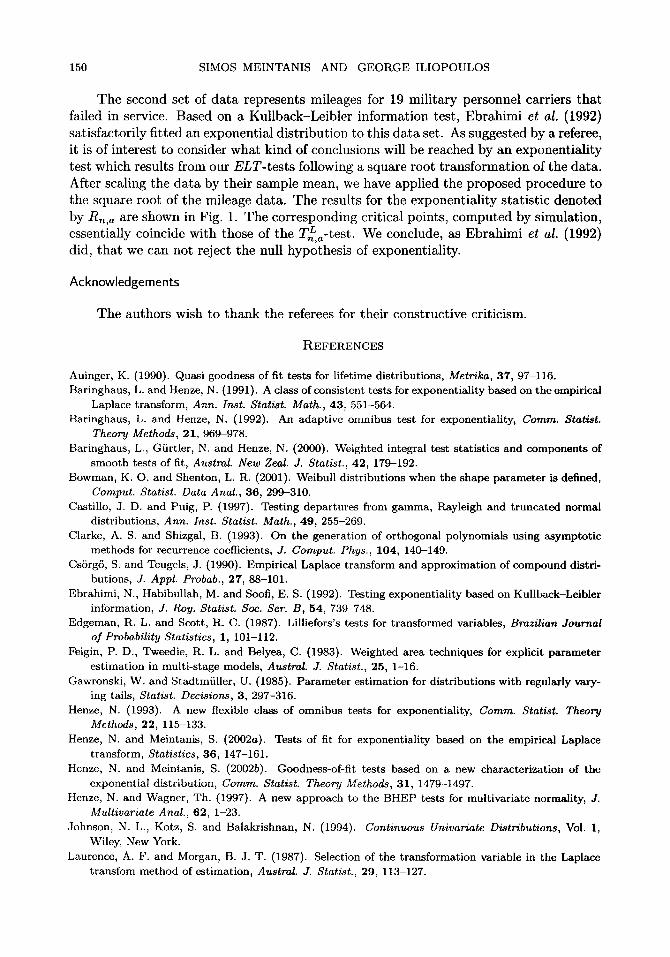
In this section we apply the proposed procedures to two data sets which have been recently employed by researchers, and compare their conclusions based on alternative methods, to the conclusions reached by our methods. The first data set represents 26 fracture toughness measurements for steels at given temperatures, and appears in Bowman and Shenton (2001), Section 4. The authors report a satisfactory fit for this data set to a two-parameter (location-scale) Weibull model with known shape parameter equal to two (the Rayleigh distribution), and estimated location parameter equal to 25.85. After subtracting the estimate of the location parameter, we have applied the proposed procedures to the toughness data and the results are shown in Fig. 1. They represent in logarithmic scale, the values of the two test statistics TLa and TMa, for several values of the weight parameter and the corresponding critical points (CR L and CR M) computed by simulation. Regardless of the choice of a and the estimation method for ~ (note that TLa and TMa are almost identical), the figure reveals a satisfactory fit, which is in agreement with the conclusions of Bowman and Shenton (2001) reached by a classical X 2 test.

%CR L

- . i ~" ,~ -~

Tmn

I ,0 2.0 3.0 4.0 S . ~ 6.0 7,0 9.0 9.0 10.0 WEIGHT PARAMETER

Fig. 1. Values of the test statistics and critical points for the fracture toughness and the mileage data.

150 SIMOS MEINTANIS AND GEORGE ILIOPOULOS

The second set of data represents mileages for 19 military personnel carriers that failed in service. Based on a Kullback-Leibler information test, Ebrahimi et al. (1992) satisfactorily fitted an exponential distribution to this data set. As suggested by a referee, it is of interest to consider what kind of conclusions will be reached by an exponentiality test which results from our ELT-tests following a square root transformation of the data. After scaling the data by their sample mean, we have applied the proposed procedure to the square root of the mileage data. The results for the exponentiality statistic denoted by Rn,a are shown in Fig. 1. The corresponding critical points, computed by simulation, essentially coincide with those of the Tia- tes t . We conclude, as Ebrahimi et al. (1992) did, that we can not reject the null hypothesis of exponentiality.

Acknowledgements

The authors wish to thank the referees for their constructive criticism.

REFERENCES

Auinger, K. (1990). Quasi goodness of fit tests for lifetime distributions, Metrika, 37, 97-116. Baringhaus, L. and Henze, N. (1991). A class of consistent tests for exponentiality based on the empirical

Laplace transform, Ann. Inst. Statist. Math., 43, 551-564. Baringhaus, L. and Henze, N. (1992). An adaptive omnibus test for exponentiality, Comm. Statist.

Theory Methods, 21, 969-978. Baringhaus, L., Giirtler, N. and Henze, N. (2000). Weighted integral test statistics and components of

smooth tests of fit, Austral. New Zeal. J. Statist., 42, 179-192. Bowman, K. O. and Shenton, L. R. (2001). Weibull distributions when the shape parameter is defined,

Comput. Statist. Data Anal., 36, 299-310. Castillo, J. D. and Puig, P. (1997). Testing departures from gamma, Rayleigh and truncated normal

distributions, Ann. Inst. Statist. Math., 49, 255-269. Clarke, A. S. and Shizgal, B. (1993). On the generation of orthogonal polynomials using asymptotic

methods for recurrence coefficients, J. Comput. Phys., 104, 140-149. CsSrg6, S. and Teugels, J. (1990). Empirical Laplace transform and approximation of compound distri-

butions, J. Appl. Probab., 27, 88-101. Ebrahimi, N., Habibullah, M. and Soofi, E. S. (1992). Testing exponentiality based on Kullback-Leibler

information, J. Roy. Statist. Soc. Set. B, 54, 739-748. Edgeman, R. L. and Scott, R. C. (1987). Lilliefors's tests for transformed variables, Brazilian Journal

of Probability Statistics, 1, 101-112. Feigin, P. D., Tweedie, R. L. and Belyea, C. (1983). Weighted area techniques for explicit parameter

estimation in multi-stage models, Austral. J. Statist., 25, 1-16. Gawronski, W. and Stadtmiiller, U. (1985). Parameter estimation for distributions with regularly vary-

ing tails, Statist. Decisions, 3, 297-316. Henze, N. (1993). A new flexible class of omnibus tests for exponentiality, Comm. Statist. Theory

Methods, 22, 115-133. Henze, N. and Meintanis, S. (2002a). Tests of fit for exponentiality based on the empirical Laplace

transform, Statistics, 36, 147-161. Henze, N. and Meintanis, S. (2002b). Goodness-of-fit tests based on a new characterization of the

exponential distribution, Comm. Statist. Theory Methods, 31, 1479-1497. Henze, N. and Wagner, Th. (1997). A new approach to the BHEP tests for multivariate normality, J.

Multivariate Anal., 62, 1-23. Johnson, N. L., Kotz, S. and Balakrishnan, N. (1994). Continuous Univariate Distributions, Vol. 1,

Wiley, New York. Laurence, A. F. and Morgan, B. J. T. (1987). Selection of the transformation variable in the Laplace

transfom method of estimation, Austral. J. Statist., 29, 113-127.


Rayner, J. C. W. and Best, D. J. (1989). Smooth Tests of Goodness of Fit, Oxford University Press, New York.

Yao, Q. and Morgan, B. 3. T. (1999). Empirical transform estimation for indexed stochastic models, J. Roy. Statist. Soc. Ser. B~ 61, 127-141.

tests of fit for the rayleigh distribution based on the empirical

Documents