The Activity and Performance of Finnish Equity Funds -Applying the Active Share Method

Economics

Master's thesis

Samu Pirinen

2011

Department of EconomicsAalto UniversitySchool of Economics

The Activity and Performance of Finnish Equity Funds

Applying the Active Share method

Master’s thesis

Samu Pirinen

1.6.2011

Economics

Approved by the Head of the Economics Department __.__.2011 and awarded

the grade

_______________________________________________________

1. examiner 2.examiner

Aalto University School of Economics ABSTRACT

Department of Economics 1.6.2011

Master’s Thesis

Samu Pirinen

THE ACTIVITY AND PERFORMANCE OF FINNISH EQUITY FUNDS Applying the Active Share method

Purpose of the study

This thesis concentrates on Finnish equity funds investing in Finland, Nordic Countries and

Europe. The objective is to determine the level of active management in the Finnish equity

market and the performance and expenses related to different activity levels. The objective is

also to examine closet indexing in the Finnish equity market.

Data and methodology

The data in this thesis is from the first quarter of 2008 to the third quarter of 2010. Mutual

fund holdings are from Investment Research Finland Ltd. and funds’ annual and quarterly

reports. Benchmark index holdings are from MSCI Barra and NASDAQ OMX. All the net

asset values for the funds and benchmark indices are from Investment Research Finland Ltd.

Total Expense Ratios are from the Finnish Mutual Fund Reports.

The level of active management is determined by using Active Share and tracking error.

Active Share measures the amount of fund holdings that differ from the benchmark index

holdings and tracking error calculates how much the fund’s daily returns deviate from the

benchmark index returns.

Results

The Finnish equity funds are quite active since less than 40% of the fund assets are on average

invested according to benchmark indices. The equity funds investing in Finland are clearly the

most passive compared to the funds investing in Nordic Countries and Europe.

The average performance of the Finnish equity funds increases as the level of activity

increases. In addition, the most active funds performed the best within every fund group with

different investment scopes.

There exist several closet indexing funds in the Finnish equity fund market. These funds also

charge substantial fees compared to their activity levels.

The average Total Expense Ratio increases with the level of active management i.e. more

active funds charge higher fees.

Keywords

Equity fund, Active Share, tracking error, active management, closet indexing

Table of Contents

1. Introduction ............................................................................................................................. 1

1.1 Background .................................................................................................................................... 2

1.2 Motivation of the study ................................................................................................................. 2

1.3 The objective and limitations of the study .................................................................................... 4

1.4 Research methodology .................................................................................................................. 5

1.5 Structure of the study ................................................................................................................... 6

2 Theoretical framework for portfolio management ...................................................................... 7

2.1 Mean-variance theory ................................................................................................................... 7

2.2 The applications of mean-variance theory .................................................................................... 7

2.3 Portfolio analysis ........................................................................................................................... 8

2.4 Common problems with mean-variance theory ........................................................................... 9

2.5 Efficient market hypothesis ......................................................................................................... 10

2.6 Carhart’s four-factor model ........................................................................................................ 12

3 Portfolio management ............................................................................................................. 14

3.1 Previous studies on portfolio management ................................................................................ 14

3.2 Active fund management ............................................................................................................ 16

3.3 Passive fund management .......................................................................................................... 19

3.4 Measures of active management ................................................................................................ 20

3.4.1 Tracking error ....................................................................................................................... 20

3.4.2 Active Share .......................................................................................................................... 24

3.4.3 Other measures .................................................................................................................... 26

4 Data and research methodology .............................................................................................. 30

4.1 Data ............................................................................................................................................. 30

4.1.1 Holdings data for the benchmark indices ............................................................................. 31

4.1.2 Holdings data for the funds .................................................................................................. 32

4.2 Methods ...................................................................................................................................... 33

4.3 Performance measures ............................................................................................................... 35

4.3.1 Sharpe ratio .......................................................................................................................... 35

4.3.2 Treynor ratio ......................................................................................................................... 36

5 Empirical results ...................................................................................................................... 37

5.1 Active Share ................................................................................................................................. 37

5.1.1 Distribution of funds to different activity levels based on Active Share ............................... 37

5.1.2 Performance measures ......................................................................................................... 40

5.1.3 Comparison between the level of active management and Total Expense Ratio ................ 44

5.2 Active Share & Tracking error ..................................................................................................... 47

5.2.1 Distribution of funds to different activity levels based on Active Share and tracking error . 47

5.2.2 Performance measures ......................................................................................................... 50

5.2.3 Comparison between the level of active management and Total Expense Ratio ................ 52

6 Conclusions ............................................................................................................................. 55

Appendices ................................................................................................................................ 59

References ................................................................................................................................. 60

List of Tables and Graphs

Table 1: An example of holdings data for one mutual fund and one benchmark index on one

period of time………………………………………………………………………………... 59

Table 2: Funds with different investment scopes distributed in Active Share classes...…...... 38

Table 3: Average Active Shares for funds in the sample...………………………………...... 40

Table 4: Average benchmark-adjusted Sharpe and Treynor ratios in Active Share classes for

funds with different investment scopes...………………………………………………….… 41

Table 5: Average Active Shares, tracking errors and benchmark-adjusted Sharpe and Treynor

ratios for funds in the sample………...…………………………………………………….... 43

Table 6: Total Expense Ratios in Active Share classes for the funds with different investment

scopes………….......……………………………………………………………………….... 44

Table 7: Funds distributed in different categories based on Active Share and tracking

error.......................................................................................................................................... 47

Table 8: Funds with different investment scopes distributed in different categories based on

Active Share and tracking error...………………………………………………………….... 48

Table 9: Three-year average Active Shares and tracking errors for Finnish equity funds...... 49

Table 10: Average benchmark-adjusted Sharpe and Treynor ratios in different categories

based on Active Share and tracking error...………………………………………………..... 50

Table 11: Average Total Expense Ratios in different categories based on Active Share and

tracking error..……………………………………………………………………………...... 52

Table 12: Average Total Expense Ratios for funds with different investment scopes

distributed in categories based on Active Share and tracking error..………………………... 53

Graph 1: Benchmark-adjusted Sharpe ratios in different Active Share levels..……………... 42

Graph 2: Total Expense Ratios in different Active Share levels..…………………………. 46

1

1. Introduction

The basic idea between mutual funds is that they pool investments from a large number of

investors and then invest the money in different types of instruments such as stocks, bonds

and short-term money market instruments. In Finland the mutual funds are divided into five

categories; equity funds, bond funds, money market funds, asset allocation funds and

alternative funds. Mutual fund’s operation is guided by the investment policy of the fund

which determines the guidelines for the investments available for the fund. Eventually, it is

the fund manager who is responsible for following the investment policy when making

investment and diversification decisions.

Fund managers have two different ways to exercise their business. They can apply very active

fund management policy or on the other hand they may be more passive. Passive fund

management can be considered as replicating the benchmark index whereas active fund

management is determined as the deviations from the passive indexing approach. Passively

managed funds are often a cheap way to invest in mutual funds and they also offer the

advantage of diversification. Actively managed funds are more expensive in terms of

administration fees and therefore they are also expected to add value relative to the

benchmark index. This will be done by exploring the markets and actively trying to

differentiate the fund holdings from the benchmark index holdings.

Investors investing in funds seek diversification but those investing in actively managed funds

also seek expertise from the fund managers who are assumed to have a more comprehensive

view of the current market situation than investors themselves. Investors assume that fund

managers can generate higher returns by finding attractive investment opportunities. This is

the most important reason why investors decide to invest in mutual funds.

2

1.1 Background

The Finnish mutual fund market was created in 1987 when the law of Finnish mutual funds

was introduced. In the early stages the development of the market was slow but the growth

accelerated in the late 1990s. The development of the Finnish mutual fund market was rapid

for a decade until the global financial crisis hit the markets in year 2007. After the massive

drop the markets started to recover and at the end of 2010 the markets were almost at the

same level than before the financial crisis. (Finnish Mutual Fund Report, 12/2010)

According to Finnish Mutual Fund Report, the distribution of total assets under management

in Finnish mutual funds i.e. funds registered in Finland at the end of 2010 was as follows;

equity funds represented 39,7% (24.4 billion euros) of total assets, bond funds 29,0% (17.8

billion euros), money market funds 16,7% (10.2 billion euros), asset allocation funds 13,1%

(8.1 billion euros) and alternative funds 1,5% (944 million euros). From the fund classes that

are included in this thesis, equity funds investing in Finland represents 19,9% (4.9 billion

euros) of the total assets in all equity funds, equity funds investing in Nordic Countries 24,9%

(6.1 billion euros) and equity funds investing in Europe 24,4% (6.0 billion euros). The total

assets under management in Finnish funds were 61.5 billion euros at the end of 2010. All in

all, the Finnish mutual fund industry covers considerable amount of assets and therefore it is

convenient to study the action of this industry in more detail.

1.2 Motivation of the study

Even though the studies concerning the mutual funds have increased as the mutual funds have

become more popular, the number of mutual fund holdings studies has still remained on a low

level due to the lack of data. Nowadays, however, there exists a database in U.S. that consists

of mutual fund holdings data which has enabled researchers to examine the mutual fund

sector more comprehensively. For instance, the invention of Active Share (Cremers &

Petäjistö, 2006) was possible due to this new data. Active Share describes the fund’s level of

active management by comparing the holdings of the fund and the benchmark index.

Unfortunately there exists no collective database for Finnish mutual fund holdings data and

therefore Active Share has remained as a rather unknown concept in Finland.

3

The previous studies (see e.g. Hendricks, Patel & Zeckhauser, 1993 and Blake &

Timmermann, 1998) have applied mainly two methods when trying to measure level of active

management in mutual funds. One is the tracking error which has also been the most

traditional method. It measures how closely the fund return follows the benchmark index

return and it is calculated as the time-series standard deviation of the difference between a

fund return and its benchmark index return. However, it is inadequate to use only tracking

error (see e.g. Israelsen & Cogswell, 2007 and Cremers & Petäjistö, 2009) since very actively

managed funds can in fact generate rather low tracking error figures which in turn may lead to

misclassification of funds. Therefore judging the activity level of fund management based

only on tracking error can be misleading.

Another method applied when dividing the funds into actively and passively managed has

simply been the notification of the fund management companies. In this classification

passively managed funds contain only the index funds whereas all the other funds are

considered to be actively managed. This approach also has a fundamental problem since

several studies have shown that there exists plenty of “closet indexing” among these so called

actively managed funds. Closet indexing is referred to when a fund that is claimed to be

actively managed by the fund management company, and therefore charges high management

fees, in fact acts like an index fund by closely replicating some benchmark index.

As mentioned above, the previous studies have applied methods that actually don’t divide the

funds into actively and passively management funds based on the real activity level of fund.

Because of the closet indexing, the category of actively managed funds has contained funds

that have only replicated the benchmark indices. These funds have generated gross returns

close to benchmark indices but due to the higher management fees the net returns have

naturally been lower than the benchmark returns. Since the closet indexing funds have yielded

less than the benchmark indices, it is easy to see that these funds have actually lowered the

average return of the truly actively managed funds and therefore also lowered their chances to

outperform the index funds. Therefore it is justified to question whether the previous results

stating that the actively managed funds can’t add value relative to index funds are valid.

Since Active Share is a rather new invention, it hasn’t been applied to Finnish mutual funds.

Therefore it is interesting to see whether the outcome of this thesis will be similar to the

results that Cremers and Petäjistö (2009) obtained from the U.S. market.

4

1.3 The objective and limitations of the study

Actively and passively managed funds have been examined a lot and the majority of the

studies have concentrated to find if actively managed funds are able to beat the index funds.

For example, Liljeblom and Löflund (2000) studied this using Finnish data. The most

common result has been that the actively managed funds can’t outperform the benchmark

indices.

However, the studies have applied inadequate methods in measuring the level of active

management of the funds. In this thesis I will classify the funds depending on their real

activity level. The main focus in measuring the level of active management is on the Active

Share method which was introduced by Cremers and Petäjistö in 2006. The method indicates

how much the fund holdings differ from the benchmark index holdings. For example, Active

Share of 60% indicates that 40% of assets are invested following the benchmark index and

60% are invested by taking bets against the index. I will also apply tracking error because it is

the most traditional method applied and together with Active Share it can create a more

comprehensive picture of the level of active management in the studied funds.

The main question in the discussion of actively and passively managed funds is whether the

actively managed fund can beat the index fund. Are the actively managed funds able to yield

higher returns than the index funds? This new classification of funds based on Active Share

method will divide funds differently into active and passive categories. Therefore it is

interesting to see if this classification yields the same results as the previous studies that the

passively managed funds outperform the actively managed funds. On the other hand, the

results may show that the truly actively managed funds can in fact outperform the index funds

and therefore add value relative to the index.

I will also study how closely the level of active management and the Total Expense Ratio

(TER) are related in the sample applied in this thesis. The activeness of the management

should determine the amount of fees charged and therefore I will compare the funds’ Total

Expense Ratios to the levels of Active Shares and tracking errors in order to clarify whether

the investors are getting what they are paying for.

5

In addition, I will search for fund categories that contain closet indexing funds and determine

whether these funds have underperformed the benchmark indices as assumed by the theory.

The closet indexing funds are very inefficient for investors and therefore I will determine

whether these kinds of funds exist in the Finnish mutual fund market.

This thesis concentrates on Finnish equity fund market, and more specifically on the equity

funds investing in Finland, Nordic Countries and Europe. The sample in my thesis consists of

64 equity funds from which 25 invest in Finland, 14 in Nordic Countries and 25 in Europe.

My sample represents the vast majority of the Finnish funds investing in Finland, Nordic

Countries and Europe. However, the period applied in this thesis is only three years and

therefore the results should be interpreted with some caution.

1.4 Research methodology

In this thesis I will apply quantitative methods in order to measure the activity and

performance levels of the funds included in my sample. The levels will be determined with

different key ratios and finally these figures will be used to categorize the funds.

The categorization into different classes based on the level of activity will be accomplished in

two ways. First, I will use only Active Share and classify the funds in four categories. The

first category contains the funds with Active Share of 0-25%, second 25-50%, third 50-75%

and fourth 75-100%. The funds in the first category represent the most passive part of the

funds, whereas the fourth category contains the most active funds. In the second

categorization method Active Share is combined with tracking error. Active Share applies the

same categories and tracking error divides the funds into five categories in which the

boundaries of tracking error of are 3 – 6%, 6 – 9%, 9 – 12%, 12 – 15% and 15 – 18%. The

level of active management is higher when Active Share and tracking error increase.

After the categorization I will study the average fund performance between different

categories. The objective is to study whether the level of active management determines the

fund performance. The methods applied in this thesis to determine level of active

management divide the funds into different categories based on the real level of active

6

management and therefore the categorization differs from the previous studies. Therefore the

thesis will be able to answer the fundamental question; Are the truly actively managed funds

able to outperform the index funds?

All the fund performances are compared to benchmark indices and therefore all the figures are

presented relative to the index. The performance of the funds will be determined by applying

two risk-adjusted performance measures; Sharpe and Treynor ratio. The period applied in this

thesis is from the first quarter of 2008 to the third quarter of 2010 and therefore I will use

three-year annualized Sharpe and Treynor figures. Per annum figures make all the funds and

benchmark indices comparable and indicate how the investments have performed on a yearly

basis.

1.5 Structure of the study

The remaining part of this thesis is structured as follows. In chapter 2 I will introduce the

theoretical background for portfolio management. Chapter 3 describes the fund management

including both active and passive fund management. Data and research methodology are

introduced in chapter 4. In chapter 5 I will present the empirical results of the study. Finally,

in chapter 6 I will draw the conclusions and give some suggestions for further studies.

7

2 Theoretical framework for portfolio management

This chapter introduces the theoretical background for portfolio management. First, I will

discuss the mean-variance theory and the applications of the theory. Next, I will introduce the

concept of portfolio analysis and the common problems concerning the mean-variance theory.

Then, I will go through the efficient market hypothesis and the Carhart’s four factor model.

2.1 Mean-variance theory

Modern Portfolio Theory is an investment theory originally introduced by Harry Markowitz

(1952). Markowitz argued that there are only two relevant elements when selecting portfolios;

the expected or average rate of return and the risk. Markowitz proposed to measure the risk of

a security by the variance (standard deviation) of its returns and he formulated the portfolio

problem as a choice of the mean and variance of a portfolio of assets. The basic concept in

this mean-variance theory was to maximize the expected return of the portfolio for a given

amount of risk or consequently minimize the risk for a given level of expected return. These

combinations of assets are called efficient portfolios which construct the efficient frontier.

The theory also states that by investing in more than one stock, an investor can diversify the

risk of the portfolio on a level that is lower than any individual security in the portfolio. The

fundamental idea is that the assets should not be selected into the portfolio based on their

individual characteristics. Rather, an investor needs to estimate how each security co-moves

with all the other securities. This way it is possible to construct a portfolio with the same

expected return and less risk than a portfolio constructed by ignoring the interactions between

the securities. (Markowitz, 1952)

2.2 The applications of mean-variance theory

Markowitz’s ideas have been applied both in theory and in practice of financial markets.

However, the Modern Portfolio Theory has rarely been implemented and Elton, Gruber and

Padberg (1976) state that there are three main reasons for that. First, it is difficult to estimate

the type of input data necessary. Second, the risk-return tradeoffs are challenging for portfolio

managers to understand. Third, generating efficient portfolios requires both time and money.

8

Many researchers have attempted to improve the model of modern portfolio theory. The mean

and variance of return of a portfolio is a simplification and therefore Elton and Gruber (1999)

included additional moments in order to describe more comprehensively the distribution of

returns of the portfolio. Tobin (1958) developed necessary conditions on the utility function

of investors and on the return distribution of assets that would result in mean-variance theory

being optimal. Lee (1977) and Kraus and Litzenberger (1976) offered alternative portfolio

theories that included skewness of the distribution of return. Elton and Gruber (1974)

constructed theories which were accurate for more realistic descriptions of the distribution of

return.

Nevertheless, mean-variance theory has remained the cornerstone of modern portfolio theory

despite these other alternatives. This persistence is not due to the realism of the utility or

return distribution assumptions that are necessary for it to be correct. Rather, it is generally

believed that there are two reasons for its persistence. First, mean-variance theory itself places

large data requirements on the investor, and there is no evidence that adding additional

moments improves the desirability of the portfolio selected. Second, the implications of

mean-variance portfolio theory are well developed, widely known and have great intuitive

appeal. (Elton & Gruber, 1997)

As the above discussion shows, the mean-variance theory has retained its position as the

leading application of modern portfolio theory, and this is why it will also be applied as a

theoretical framework of this thesis.

2.3 Portfolio analysis

In relation to his earlier ideas, Markowitz (1959) stated that a good portfolio is more than a

long list of stocks and bonds. The idea was that portfolio is a balanced whole providing

protection and opportunities to the investor. Therefore the investor should build toward an

integrated portfolio that best suits his needs. First step in portfolio analysis is to analyze the

information concerning the individual securities. This information includes the past

performance of individual securities as well as the beliefs of security analysts concerning the

future performances. Portfolio analysis leads to conclusions concerning the constructed

9

portfolio as a whole. The main purpose of this analysis is to find the portfolio that best meets

the objectives of the investor.

Investors try to maximize the expected returns and minimize the return variance. Therefore

they are only interested in efficient portfolios. Markowitz (1952) indicated that efficient

portfolios take the form of a parabola in the mean-variance space. All the efficient portfolios

lie on the efficient frontier and therefore the investor should choose a portfolio on the efficient

frontier based on one’s individual risk and return preferences. The portfolio with the lowest

variance on the efficient frontier is called the minimum variance portfolio. Furthermore, the

minimum variance frontier contains the set of portfolios that offers the lowest risk at any level

of return.

The efficient frontier line has two end-points: the one with lower variance is called the global

minimum variance portfolio and the other is the maximum return portfolio. The efficient

frontier consists of the envelope curve of all portfolios that lie between these two points. The

efficient frontier is a concave function because it is a combination of several securities or

portfolios. (Markowitz, 1952)

2.4 Common problems with mean-variance theory

Even though mean-variance theory is widely acknowledged, there are still some problems

involved with the theory. In this chapter I will introduce the main problems discussed in the

academic literature.

The mean-variance portfolio theory was developed to find the optimal portfolio for an

investor concerned with return distribution over one period. The mean return and the variance

of return are estimated for each asset in the portfolio over the single period. The correlations

between all pairs of assets are also estimated for this same decision period. Therefore one of

the major theoretical problems that has been analyzed is how the single-period problem

should be handled if the investor’s true problem includes several periods. (Elton & Gruber,

1997)

Mossin (1968), Fama (1970b), Hakansson (1970, 1974) and Merton (1990) have focused on

this particular problem. They found that the multi-period problem can be solved as a sequence

10

of single-period problems under various assumptions. However, they also found that the

optimal portfolio would be different from that selected if only one period was examined. The

reason is that the multi-period utility function differs from the single-period utility function.

One assumption underlying most multi-period portfolio analyses is the independence of

returns between periods. However, there is a significant amount of research (see e.g.

Campbell & Shiller, 1988 and Fama & French, 1989) that indicates the connection between

different periods for mean returns and variances. They also show that mean returns and

variances are functions of easily observable variables.

Some problems have also been associated with the portfolio optimization. Jorion (1985)

argues that the optimal portfolio based on the sample performs quite often much poorer

outside the sample. He points out that the sample period optimal portfolio is sometimes

dominated even by very simple methods, like equally weighted index. In addition, Jorion

states that the optimal portfolio is very volatile because the asset weightings are extremely

sensitive to variations in expected returns. Moreover, optimal portfolios are not necessarily

well diversified since the solution of the optimization problem is often a corner solution. This

means that most of the investment weightings are zero and large proposition of assets are

allocated to countries with relatively small capital markets and high average returns.

2.5 Efficient market hypothesis

Efficient market hypothesis is closely related to Modern Portfolio Theory. Efficient market

hypothesis was originally developed by Eugene Fama in 1970. Efficient market hypothesis

states that it is impossible to beat the market regularly because stock market efficiency causes

existing stock prices to always incorporate and reflect all available information. This means

that securities are always traded at fair values and investors aren’t able to purchase

undervalued or sell overvalued securities. Consequently, the efficient market hypothesis states

that it is impossible to outperform the market using expert stock selection or market timing.

Investor can gain higher returns than the market by investing in riskier securities but it can’t

beat the market on risk-adjusted basis.

11

As mentioned above, the efficient market hypothesis states that stock prices reflect all

available information. Fama (1970a) classified market efficiency into three categories by the

notion of what is meant by the term “all available information”:

The weak-form hypothesis asserts that stock prices reflect all information that can be derived

by examining market trading data such as the history of past prices, trading volume or short

interest. Past stock price data are publicly available and virtually costless to obtain.

The semistrong-form hypothesis states that stock prices reflect all publicly available

information regarding the prospects of a firm. Such information includes, in addition to past

prices, for example balance sheet composition and earnings forecasts.

The strong-form hypothesis states that stock prices reflect all information relevant to the

firm. This includes also the insider information of the company.

According to Efficient Market Hypothesis, actively managed funds can’t create value for

investors because markets are working perfectly. This suggests that all the research done by

the active managers is simply waste of resources and just lowers the funds’ returns after fees.

The basic implication from Efficient Market Hypothesis is that instead of using investing in

actively managed funds the investors should invest in passive index funds since they will

generate higher risk-adjusted returns after fees. However, several studies (e.g. Dreman &

Berry, 1995 and Lo & MacKinlay, 2001) have argued that the markets aren’t perfect and

suggested that it is possible for actively managed funds to obtain higher returns than the

passive index funds by actively researching the markets. In this thesis I will also try to

contribute to this discussion from my behalf.

As mentioned earlier, Efficient Market Hypothesis states that it is impossible to outperform

the market using expert stock selection. There are several models which try to explain the

behavior in mutual fund performance. Next, I will introduce probably the most widely

accepted model trying to determine whether the fund manager has been able to generate risk-

adjusted returns by having the skill to pick right stocks.

12

2.6 Carhart’s four-factor model

The behavior of mutual fund performance is widely studied in the academic world. There are

several different models trying to find the factors that explain the behavior in mutual fund

returns. Capital Asset Pricing Model (CAPM) applies only beta that describes the relationship

between the returns of the fund and the market. Fama and French developed the three-factor

model which takes into account the size and book-to-market factors in addition to the market

beta introduced by CAPM. This chapter introduces the four-factor model developed by Mark

Carhart in 1997. The model is derived as follows:

�i-Rf = �i + m��m − �f� + s�s + b�b + o�o

where

Ri – Rf is the fund’s excess return

Rm – Rf is the market factor return

Rs is the size factor return

Rb is the book-to-market factor return

Ro is the momentum factor return

αi is the fund’s risk-adjusted return

βm is the fund’s market beta

βs is the fund’s size beta

βb is the fund’s book-to-market beta

βo is the fund’s momentum beta

Fund’s excess return is the fund return minus the risk-free return and the market factor return

is the average market return in excess to the risk-free return. The size factor return means the

return to a fund of small-cap stocks less the return of large-cap stocks. This comes from the

observation that small-cap stocks have performed better than the market as a whole. The

book-to-market factor return is defined as the return to a fund of the stocks with a high ratio

13

of book-to-market value minus the return of the stocks with a low ratio of book-to-market

value. The reason for applying the book-to-market factor is that the stocks with high book-to-

market ratio i.e. the value stocks have also outperformed the market. The momentum factor

return means the return to a fund of the stocks that outperformed the market in the past less

the return of the stocks that underperformed the market in the past. This comes from the

observation that the stocks that have outperformed the market in the previous period tend to

outperform the market in the next period also.

The betas for market, size, book-to-market and momentum factors define the sensitivities of

how much the factor returns have generated excess return for the fund. For example, the

momentum beta of 2 has twice as large effect on the fund than the beta of 1. After the returns

attributable to different factors have been determined, the alpha accounts for the rest of the

fund’s excess return. Alpha measures how well the fund manager has performed beyond the

investment strategies involved in the model and therefore the alpha determines whether the

fund manager have had the skill to pick the right stocks.

For example, if a fund manager invests in value stocks and returns 10% when benchmark

index returns 5%, it seems that the fund manager has performed very well. But if the value

stocks in general returned 15% then the fund manager has underperformed the value stocks on

average. Four-factor model explores this phenomenon and determines whether the fund

manager really has exceptional skills in picking stocks and this way can generate alpha.

The four-factor model interprets how the fund manager has generated the excess returns. Has

the fund manager taken extra risk which can be seen in the high market beta or has he

employed investment strategy where the amount of value stocks is increased which leads to

higher book-to-market beta?

14

3 Portfolio management

In this chapter I will introduce portfolio management. First I will go through the main studies

concerning the concept of portfolio management and then I will describe individually both

active and passive styles of portfolio management. Finally I will introduce the different

measures of active management.

3.1 Previous studies on portfolio management

Portfolio management is divided into two separate categories: active portfolio management

and passive portfolio management. The conversation around active and passive portfolio

management has continued for decades. The main question has been whether the actively

managed funds are able to produce higher returns than their benchmark indices?

The vast majority of studies concerning the performance of active and passive portfolio

management suggest that active funds on average underperform their benchmark indices after

fees. Even the earliest researchers (see e.g. Sharpe, 1966 and Jensen, 1968) reported

underperformance on a risk-adjusted basis of actively managed funds against the benchmark.

Sharpe (1991) also states that active funds must generate average returns equal to those

derived from passive strategies. He argues that the market return must equal a weighted

average of the returns on both active and passive segments of the market. Since overall

market and passive returns should be the same, Sharpe notes that the active returns before fees

must be the same too. Therefore the return of active management should be lower after fees.

Blake and Timmermann (1998) found evidence on underperformance of actively managed

funds during 1972-1995, while Hendricks, Patel and Zeckhauser (1993) reported same kind of

underperformance for active equity funds during 1974-1988. Elton, Gruber and Blake (1993)

studied funds’ alphas, which are generated with successful stock picking, i.e. the amount of

fund return that exceeds the benchmark index return after the different factor returns are

excluded from the fund excess return. They found that there was no evidence on positive

alphas for actively managed funds against the benchmark indices. Davis (2001) compared

different investment styles among active equity funds and found that none of these styles were

able to generate positive abnormal returns during 1965-1998. He also wondered why most of

the funds were reluctant to own value stocks when these stocks had higher average returns.

15

Swedroe (1998) states that the research and trading expenses together with tax consequences

make it too hard for active managers to constantly beat the benchmark index. Gruber (1996)

agrees this by reporting that even though active management can add value, the expenses

more than offset the value added and therefore the actively managed funds have negative

performances compared to a set of indices. Carhart (1997) also argues that only the best

actively managed funds earn back the fees they charge, while the most funds underperform on

average by the magnitude of their investment expenses. Elton and Gruber (2003) are a bit

more optimistic stating that in order for active management to be effective it has to overcome

the following higher costs: costs of forecasting, costs of transactions and costs of diversifiable

risk because investors must be compensated for taking higher risk.

There has also been lot of studies concerning the performance of well-known indices and

index funds. For example, Shefrin (2000) studied the performance of Vanguard 500 index

fund, which tracks the S&P 500 index, during 1977-1997. He discovered that the Vanguard

500 index outperformed over 83 percent of all funds during this twenty-year period. Malkiel

and Radisich (2001) support this evidence by stating that S&P 500 index outperformed almost

90 percent of all actively managed equity funds.

There are also studies that have explored the active fund management in Finnish market.

Kasanen and Kinnunen (1990) found evidence that also in Finland the actively managed

funds underperformed the benchmark indices during 1988-1989. Another research with

Finnish data by Liljeblom and Löflund (2000) stated that only few funds were able to

generate statistically significant positive abnormal returns during 1991-1995. Furthermore,

according to the Finnish Mutual Fund Report representing the situation on 31.12.2010, the

Finnish equity funds investing in Finland underperformed the OMX Helsinki CAP GI index

on average when measured with 12 month return.

There has also been a lot of discussion about the activity level of the funds that are supposed

to be actively managed. Funds that are claimed to be actively managed by fund management

companies and charge high management fees but in reality follow closely some index are

called closet indexers. Petäjistö (2010) studied closet indexing and argued that it accounts for

about one third of all mutual fund assets. He also found that closet indexing has become more

popular after the market volatility started to increase in 2007. Petäjistö suggests that the

16

reasons for increased interest in closet indexing are the recent market volatility and negative

returns. He argues that these reasons also explain the previous peak in closet indexing in

1999-2002.

Petäjistö (2010) studied also the performance of the closet indexer funds. He found that closet

indexers performed poorly against their benchmark indices. As one could predict based on the

nature of closet indexers, they largely just matched their benchmark index returns before fees.

Consequently, closet indexers underperformed the benchmark indices on average by the

amount of their fees.

As we can see from above discussion, almost all of the studies suggest that active fund

management is only waste of money since actively managed funds can’t beat the benchmark

indices on a regular basis. Even though Elton and Gruber (2003) are a bit more optimistic

towards the actively managed funds, the general opinion strongly favors the passively

managed funds.

Despite the fact that the majority of the previous studies suggest that passive fund

management contributes better results than active fund management, it is noteworthy that the

active managers still control the vast majority of the total mutual fund assets. The main reason

for this is that the actively managed funds charge higher management fees and therefore fund

management companies are more willing to offer these funds than cheaper index funds.

The following chapters will concentrate on both active and passive fund management

respectively.

3.2 Active fund management

Active fund management refers to a portfolio management strategy where the fund manager

seeks to outperform the benchmark index by deviating from it. Consequently, active

management can be defined as any deviation from passive management. To measure the

active management, one needs to calculate the amount of deviation from passive

management.

17

Active fund management is generally understood to concern all investment-related activities

of the clients’ investment assets. It involves active monitoring and professional decision

making in the best interest of the clients. The whole process of active fund management can

be divided into input and output activities. The process begins with comprehensive research in

order to obtain economic and investment data. Based on the data, the fund manager

formulates an investment strategy for the fund. Based on this investment strategy, the fund

manager determines asset allocations and applies them to the fund by purchasing and selling

securities. This way the fund manager obtains the desired exposures. After the fund manager

has constructed the portfolio, he needs to start reporting the performance of the fund for the

client. This consists of performance measures, performance analyses and reporting statement.

(Ehlern, 1997)

Fund managers apply either a top-down or bottom-up approach to the investment process. A

top-down approach begins with an asset allocation and then moves to a selection of individual

securities to meet these allocations. The most important decision in a top-down approach is

the choice of markets and currencies. Therefore the macroeconomic conditions and trends are

researched and the choice of markets and currencies are made based on the obtained data.

After the choice of markets and currencies, the best available securities will be selected.

Another alternative is the bottom-up approach which refers to the qualitative analysis solely

on individual securities. This analysis produces a selection of superior stocks from which the

fund manager selects the best securities irrespective of their national origin or currency

denomination to build a portfolio. As a result, the bottom-up approach constructs a fund with

a market and currency allocations that are random results of the securities selected. (Solnik,

1996)

An active fund manager tries to beat the fund’s benchmark one way or another. Nevertheless,

the main point for active manager is to take positions that are different from the benchmark.

There are two ways how fund holdings can differ from the benchmark: stock selection or

factor timing. Stock selection simply involves picking individual stocks that the fund manager

expects to outperform the benchmark index without changing the level of systematic risk.

Factor timing concentrates on time-varying bets on systematic risk factors such as entire

industries, sectors of the economy or more generally any systematic risk relative to the

benchmark index. (Fama, 1972)

18

Elton and Gruber (2003) divides active fund managers into three categories: market timers,

security selectors and sector selectors. Market timers change the beta on the portfolio

according to the forecasts of how the market will perform. Beta measures the fund’s risk

relative to the benchmark index. The fund managers vary the percentage of fund’s assets in

equity securities depending on their view of right timing on the stock market. Security

selectors concentrate on individual securities and aim to increase the weight of undervalued

and decrease the weight of overvalued securities. They usually apply fundamental analysis on

choosing the superior stocks. Sector selectors aim to take advantage of market trends during

different economic cycles. They try to forecast expected market developments and determine

which sectors and industries are under- and overvalued, and based on this data they rotate

their portfolios by over- and underweighting the particular sectors and industries.

As mentioned earlier, the actively managed funds attempt to outperform the benchmark index

by actively researching financial markets. This research, as well as all transactions made,

generates costs for fund management companies and therefore actively managed funds charge

higher management fees. However, dilemma arises when a fund management company

claims the fund to be actively managed but the fund manager decides to act like an index fund

manager and closely replicates the benchmark index. As mentioned earlier, these kinds of

funds are often referred as closet indexer funds.

Closet indexer funds don’t try to outperform the benchmark index but they still charge high

management fees. This is naturally the opposite of what investors are paying active managers

to do. Investors could get the same kind of portfolio but pay much less by investing separately

in a low-cost index fund and in a truly active fund. Fund managers’ performance is usually

compared to the benchmark index, so the manager has an incentive to gain at least the same

returns than the benchmark. Closet index funds generally exist because their managers believe

it is safer to track index rather than take greater risks with more active management. Petäjistö

(2010) found that closet indexing increases with market volatility and also when market goes

down. The manager’s career risk for underperformance is also greater in highly volatile

markets and down markets. Therefore Petäjistö suggests that career risk for underperformance

explains the increase in closet indexing in highly volatile markets and down markets.

(Petäjistö, 2010)

19

In this thesis I will explore whether the Finnish mutual fund market contains closet indexing

funds. I will also determine whether these funds charge too large fees compared to their levels

of active management.

3.3 Passive fund management

Fund management is called passive when the fund manager decides to track the benchmark

index instead of attempting to outperform the benchmark index. Benchmark index tracking is

also called indexing. The idea of an index fund was first presented by John Bogle in 1976. He

proposed that there should be an extremely low-cost fund available that wouldn’t attempt to

beat the average returns of the stock market. Instead Bogle suggested that the low-cost fund

should replicate the S&P 500 index.

According to the efficient market theory, stock prices are at fair levels given all available

information. Therefore buying and selling securities frequently would generate large

brokerage fees without increasing portfolio’s expected performance. In passive management

the fund is supposed to track the movements of the entire market. Passive funds consider the

current market price to be the best estimate of security’s value. Hence, passive funds don’t try

to pick undervalued securities. (Frino & Gallagher, 2001)

The management of passive funds is rather straightforward. It consists of replicating the

return of the benchmark index with a strategy of buying and holding the index stocks in the

official index proportions. The holdings of the passively managed funds are usually

rebalanced every six months or once a year. The passive fund management aims to establish a

well-diversified portfolio of securities with least possible costs. Buying and holding strategy

doesn’t require research considering the future market developments and therefore the

administrative costs of passive funds are significantly lower than those of actively managed

funds. (Frino & Gallagher, 2001)

From the investor’s point of view, the benefit from indexing is that by investing in one index

fund, it is possible to track the movements of much larger capital market. Even though the

indexing fund needs to maintain the relative weight of the individual stock in the fund

reflecting the index composition, it is less expensive than the active fund management. (Frino

& Gallagher, 2001)

20

3.4 Measures of active management

The level of active management has historically been measured with many different methods.

Tracking error has traditionally been the most used technique but the others have also been

applied on a regular basis. For instance, Active Share is a very recent method but has already

aroused interest in academic world. The most frequently applied measures are introduced

more comprehensively in the following sections.

3.4.1 Tracking error

Tracking error has traditionally been the most common way to measure active management of

a fund and therefore it has also been widely studied. It measures how closely the fund return

follows the benchmark index return. Deviations in these returns indicate how actively the

fund is managed. Tracking error is defined as the time-series standard deviation of the

difference between a fund return and its benchmark index return:

������������� = ���� !�i− �bm",

where

Ri is the return of the fund

Rbm is the return of the benchmark index

High tracking error indicates that the fund returns have deviated a lot from the returns of the

benchmark index. For instance, a tracking error of 5% means that the fund returns deviate 5%

from the benchmark index returns. If the fund contains exactly the same securities than the

benchmark, then the tracking error for the fund is 0%. Tracking error increases when the fund

holdings start to differ from the benchmark index holdings.

Ammann and Tobler (2000) claim that there are two main reasons why tracking error occurs.

Those are the attempt to outperform the benchmark index by active fund management and the

21

passive replication of the benchmark index. In active fund management the tracking error

signals how much risk the fund has taken relative to benchmark index when trying to beat the

benchmark. In passive management it evaluates the success of the benchmark index

replication.

For the investor, the tracking error figure reveals the conscious and active risk the fund is

taking and the potential to add value. High tracking error indicates that the portfolio return has

varied a lot in relation to benchmark return. Correspondingly, low tracking error tells that the

portfolio and benchmark returns have been close to each other. Actively managed funds tend

to generate higher tracking errors than those of passively managed. This is due to the fact that

active fund managers try to beat the benchmark index by constructing a fund that differs from

the benchmark index, whereas passively managed funds simply replicate the benchmark

index.

Tracking error and passive fund management

Indexing is often considered to be rather simple investment strategy since it only has to

replicate the benchmark index. However, Chiang (1998) disagrees and argues that the concept

of index fund is not as straightforward as it looks like. Even though in theory the tracking

error of the index fund should equal zero, in practice it rarely is the case. Chiang points out

that even index funds can experience so called tracking problem where they are unable to

perfectly track the movements of the benchmark index. He finds several reasons for why

passively managed funds generate tracking errors, such as transaction costs, fund cash flows,

the volatility of the benchmark, the treatment of dividends by the index and the index

composition changes. Consequently, index fund managers adopting an indexing approach

can’t guarantee that their portfolios’ performance will be identical to the benchmark index.

Keim (1999) states that the liquidity of the underlying index will also have implications for

transaction costs and hence the tracking error incurred by index funds.

Frino and Gallagher (2001) argue that given the market frictions, tracking error is unavoidable

even in passively managed funds. Many benchmark indices are market capitalization

weighted, which means that the amount of each security held in the index fluctuates

depending on the proportion of the market capitalization of the security relative to total

market capitalization of the index. Market capitalization is the market price times the shares

outstanding and therefore fluctuations in security prices cause the composition of these

22

indices to change constantly. Even though the passively managed index funds trade

automatically, the trades are often executed with slightly different timing depending on the

speed of the exchange and the trading volume in each security. Consequently, the passively

managed funds will generate tracking error.

Frino and Gallagher (2001) also point out that index funds’ replication strategy generates

transaction expenses, whereas the benchmark index is balanced without taking costs into

account. In addition, the daily values for fund and benchmark index are calculated at different

time of the day. Whereas index values are normally calculated at market close, the funds’

calculation times vary, and are ordinarily earlier during the day.

Despite these frictions, Frino and Gallagher (2001) state that tracking error is a natural way to

manage passive funds. However, the managers of passively managed funds face the dual

objective of minimizing tracking error as well as minimizing the costs incurred in tracking the

index as closely as possible. Consequently, there exists a trade-off between tracking error

minimization and transaction costs.

Fund managers usually aim for an expected return higher than the benchmark index. They

also want to have a low tracking error volatility to minimize the risk of considerably

underperforming the index. The ideal situation for fund manager is when the fund

outperforms the benchmark index every time by the same fixed amount. This way the fund

manager would be adding value over an index and the tracking error would be zero. This

method is called mean/variance analysis of tracking error and it is a common tool for

evaluating active management. (Roll, 1992)

As Roll (1992) studied the mean-variance analysis he found that it is not possible to reach

more efficient portfolio by minimizing the volatility of tracking error. Jorion (2003) also used

the mean-variance analysis when he studied active portfolios subject to a constraint on

tracking error volatility. Jorion recommended to abandon tracking error volatility

optimization and to concentrate on the total risk instead. The simplest constraint is to keep

portfolio volatility no greater than that of the benchmark.

23

Problems with the term “tracking error”

Although tracking error seems to give us good information about the fund’s management

activity, there are some problems related to this term “tracking error” since some people may

find the word “error” a bit confusing. When studying passively managed funds “error” is a

good term since the passive funds should replicate the benchmark indices and therefore

generate low tracking error figures. The term “error” then describes the error generated

between the returns of the passively managed fund and the benchmark index. On the other

hand, the term “error” is very misleading when exploring the differences in daily returns

between actively managed funds and benchmark indices. Actively managed funds try to

outperform the benchmark indices and therefore the tracking error is significantly higher than

zero. Consequently, the term “error” is not suitable to describe these daily return differences

between actively managed funds and benchmark indices.

Israelsen and Cogswell (2007) consider “differential from benchmark” to be more instructive

and constructive term than “error”. They criticize the term “error” claiming that it is natural

for high tracking error portfolios to have higher alpha than the lower tracking error portfolios.

Israelsen and Cogswell also claim that ranking portfolios by tracking error alone emphasizes

business risk. Therefore they suggest that to make portfolio rankings more sensible one

should combine alpha and tracking error into information ratio and use it with tracking error.

The concept of information ratio will be discussed later on.

Tracking error and active fund management

Cremers and Petäjistö (2009) argue that two distinct approaches to active management can

produce significantly different tracking errors. Pure stock picker fund generates alpha with the

stock selection within industries but diversifies by investing across industries. In contrast,

sector rotator fund picks entire sectors and industries that outperform the average market

while holding mostly diversified positions within those sectors. The outcome is such that the

sector rotator fund has significantly higher tracking error than the stock picker fund indicating

that the sector rotator fund is much more active. But the lower tracking error for the stock

picker comes actually from the greater diversification available.

Instead of using tracking error alone, Cremers and Petäjistö (2009) suggest that a more

comprehensive picture of active management can be achieved by including Active Share into

24

the calculations. The concept of Active Share will be discussed in more detail in the

following.

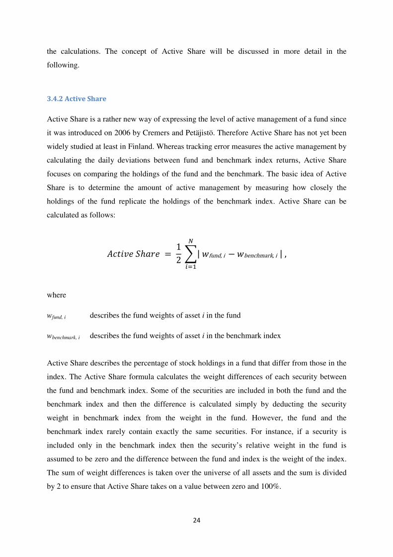
3.4.2 Active Share

Active Share is a rather new way of expressing the level of active management of a fund since

it was introduced on 2006 by Cremers and Petäjistö. Therefore Active Share has not yet been

widely studied at least in Finland. Whereas tracking error measures the active management by

calculating the daily deviations between fund and benchmark index returns, Active Share

focuses on comparing the holdings of the fund and the benchmark. The basic idea of Active

Share is to determine the amount of active management by measuring how closely the

holdings of the fund replicate the holdings of the benchmark index. Active Share can be

calculated as follows:

$��� ��ℎ��� = 12(|*fund,i−*benchmark,i|,

4

567

where

wfund, i describes the fund weights of asset i in the fund

wbenchmark, i describes the fund weights of asset i in the benchmark index

Active Share describes the percentage of stock holdings in a fund that differ from those in the

index. The Active Share formula calculates the weight differences of each security between

the fund and benchmark index. Some of the securities are included in both the fund and the

benchmark index and then the difference is calculated simply by deducting the security

weight in benchmark index from the weight in the fund. However, the fund and the

benchmark index rarely contain exactly the same securities. For instance, if a security is

included only in the benchmark index then the security’s relative weight in the fund is

assumed to be zero and the difference between the fund and index is the weight of the index.

The sum of weight differences is taken over the universe of all assets and the sum is divided

by 2 to ensure that Active Share takes on a value between zero and 100%.

25

If the fund fully replicates the benchmark index then the Active Share is 0%. This means that

the level of active management in the fund is 0% i.e. the fund is totally passive.

Correspondingly, if the fund’s holdings differ completely from the benchmark index the

Active Share equals 100% signaling that the fund is totally active. Active Share is always

between 0% and 100% for a fund that never shorts a stock or buys on margin. (Cremers &

Petäjistö, 2009)

Table 1, which is presented in appendix 1, shows an example of the data that is required to

calculate fund’s Active Share. In the table there are all the relative weights of the securities

for both the fund and the benchmark index. In Active Share calculations all the differences in

relative weights between the fund and the benchmark index are calculated together and then

multiplied by 0,5. Using the Active Share equation above we can calculate that the Active

Share for the example fund is 9,70%.

Another way to describe Active Share is to assume that there is a fund with a €10 million

portfolio and an index that contains 100 stocks. The fund manager decides to invest €10

million in the index and thereby having a pure index fund with 100 stocks. Assume the

manager eliminates half of the stocks and invests this €5 million to some other stocks. Now

the fund has an Active Share of 50% (i.e. 50% overlap with the index). If the manager decides

to invest in only 10 out of 100 stocks in the index, the fund’s Active Share will be 90% (i.e.

10% overlap with the index). According to Active Share, it is equally active to pick 10 out of

100 stocks in the index or 50 out of 500 stocks because in both cases you have an Active

Share of 90% and you choose to exclude 90% of stocks in the index from your portfolio.

Benefits of Active Share measure

Cremers and Petäjistö (2009) argue that there are two main reasons why Active Share is a

useful method to measure fund’s active management. First, since an active manager can only

add value relative to the index by deviating from it, Active Share can provide information

about fund’s potential for beating the benchmark index. A positive level of Active Share is

necessary in order for fund manager to outperform the benchmark index. Second, Active

Share can also be combined with more traditional method of measuring the active

management of a fund, tracking error. These two methods complement each other and

together they form more comprehensive way to measure active management.

26

Cremers and Petäjistö (2009) applied Active Share method to measure the active management

for all-equity funds in the U.S. They found that funds with highest Active Share exhibited

some skill and picked portfolios which outperformed their benchmarks by 2.40% per year.

After fees and transaction costs this outperformance decreased to 1.13% per year. In contrast,

funds with the lowest Active Share had poor benchmark-adjusted returns before expenses,

0.11%, and they did even worse after expenses, underperforming by -1.42%. These results

indicate that the most actively managed funds are able to beat the benchmark indices by

exploring the markets. On the other hand, the funds that replicate the benchmark indices

generate quite similar returns than the benchmarks before fees but the after fees returns are

lower than the benchmarks.

3.4.3 Other measures

Although Active Share and tracking error are the methods by which the activity of funds will

be described in my thesis, I will also present here few commonly used alternative methods.

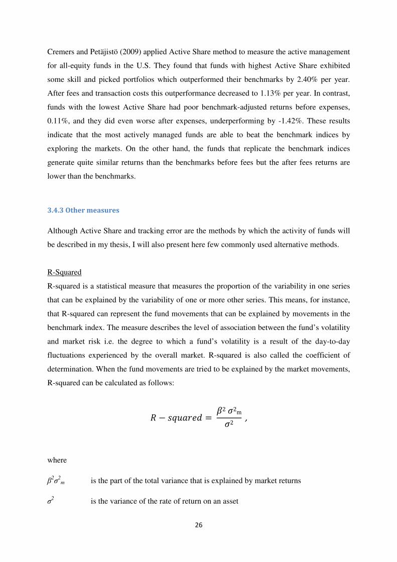
R-Squared

R-squared is a statistical measure that measures the proportion of the variability in one series

that can be explained by the variability of one or more other series. This means, for instance,

that R-squared can represent the fund movements that can be explained by movements in the

benchmark index. The measure describes the level of association between the fund’s volatility

and market risk i.e. the degree to which a fund’s volatility is a result of the day-to-day

fluctuations experienced by the overall market. R-squared is also called the coefficient of

determination. When the fund movements are tried to be explained by the market movements,

R-squared can be calculated as follows:

� − 89:���� = 2;2m;2 ,

where

β2σ

2m is the part of the total variance that is explained by market returns

σ2 is the variance of the rate of return on an asset

27

R-squared measures the correlation between a fund and benchmark index. It is calculated by

regressing the fund returns against its benchmark index returns over time. The values of R-

squared are always between 0 and 1 and the higher the value is, the greater the correlation

between the fund and the benchmark index. R-squared of 1 indicates that all movements of a

fund are completely explained by movements in the index. Correspondingly, a low R-squared

states that very few of the fund’s movements are explained by the benchmark index. For

instance, if the fund’s R-squared is measured to be 0.8, then the benchmark index explains

80% of the fund’s movements i.e. the manager correlates with the benchmark index by a

factor 80% over time. (Bodie, Kane & Marcus, 2005)

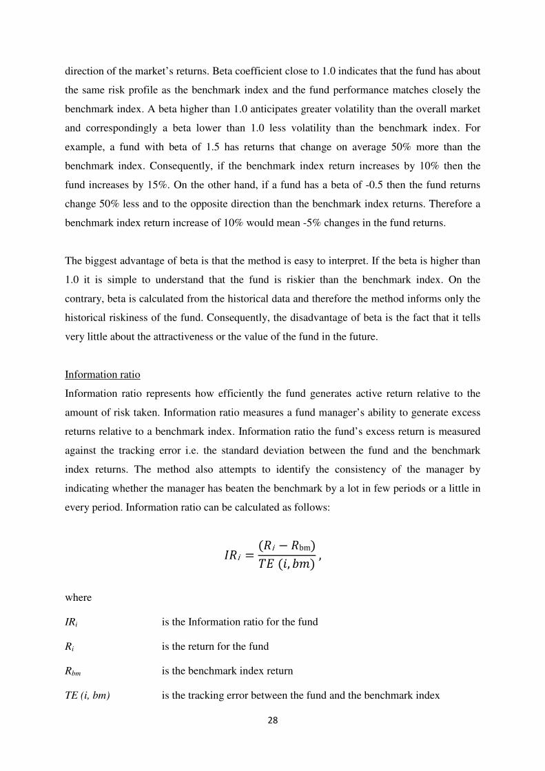
Beta Coefficient

Beta coefficient is used to describe the relation between the movements of a fund and the

market as a whole. Beta coefficient measures the risk of a fund in comparison to the risk of

the benchmark index and the risk is described by the volatility of the returns. Beta can be

calculated as follows:

i =<� (�i, �bm�=����bm� ,

where

βi is the beta coefficient of the fund

Cov (Ri, Rbm) is the covariance between the fund and benchmark index returns

Var (Rbm) is the variance of benchmark index returns

The beta coefficient above is the same as the beta obtained from the linear regression analysis

that is used in the Capital Asset Pricing Model. CAPM determines the asset’s required rate of

return and the beta coefficient represents the asset’s sensitivity to the market risk.

Positive beta coefficient indicates the fund and benchmark index generally move to the same

direction whereas negative beta means that the fund returns tend to move in the opposite

28

direction of the market’s returns. Beta coefficient close to 1.0 indicates that the fund has about

the same risk profile as the benchmark index and the fund performance matches closely the

benchmark index. A beta higher than 1.0 anticipates greater volatility than the overall market

and correspondingly a beta lower than 1.0 less volatility than the benchmark index. For

example, a fund with beta of 1.5 has returns that change on average 50% more than the

benchmark index. Consequently, if the benchmark index return increases by 10% then the

fund increases by 15%. On the other hand, if a fund has a beta of -0.5 then the fund returns

change 50% less and to the opposite direction than the benchmark index returns. Therefore a

benchmark index return increase of 10% would mean -5% changes in the fund returns.

The biggest advantage of beta is that the method is easy to interpret. If the beta is higher than

1.0 it is simple to understand that the fund is riskier than the benchmark index. On the

contrary, beta is calculated from the historical data and therefore the method informs only the

historical riskiness of the fund. Consequently, the disadvantage of beta is the fact that it tells

very little about the attractiveness or the value of the fund in the future.

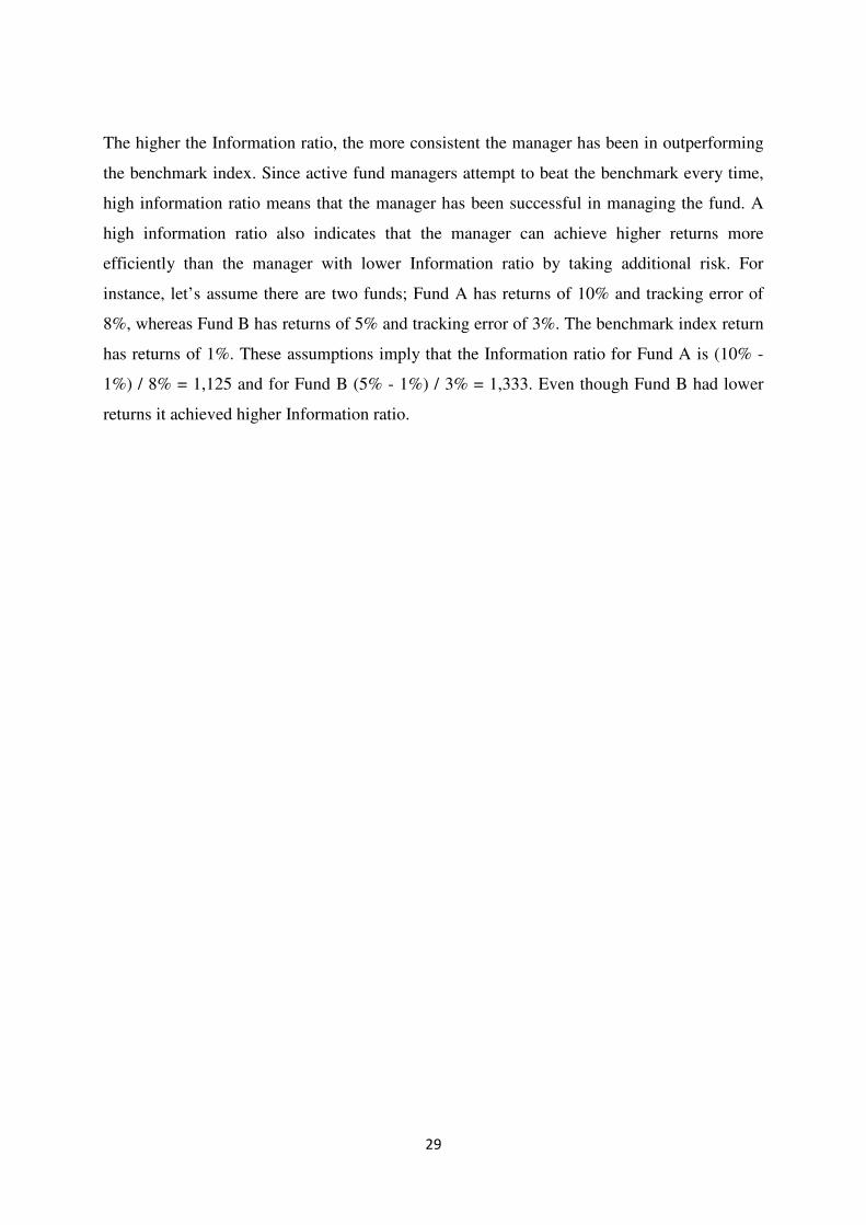
Information ratio

Information ratio represents how efficiently the fund generates active return relative to the

amount of risk taken. Information ratio measures a fund manager’s ability to generate excess

returns relative to a benchmark index. Information ratio the fund’s excess return is measured

against the tracking error i.e. the standard deviation between the fund and the benchmark

index returns. The method also attempts to identify the consistency of the manager by

indicating whether the manager has beaten the benchmark by a lot in few periods or a little in

every period. Information ratio can be calculated as follows:

>�i =(�i− �bm�����, ?@�,

where

IRi is the Information ratio for the fund

Ri is the return for the fund

Rbm is the benchmark index return

TE (i, bm) is the tracking error between the fund and the benchmark index

29

The higher the Information ratio, the more consistent the manager has been in outperforming

the benchmark index. Since active fund managers attempt to beat the benchmark every time,

high information ratio means that the manager has been successful in managing the fund. A

high information ratio also indicates that the manager can achieve higher returns more

efficiently than the manager with lower Information ratio by taking additional risk. For

instance, let’s assume there are two funds; Fund A has returns of 10% and tracking error of

8%, whereas Fund B has returns of 5% and tracking error of 3%. The benchmark index return

has returns of 1%. These assumptions imply that the Information ratio for Fund A is (10% -

1%) / 8% = 1,125 and for Fund B (5% - 1%) / 3% = 1,333. Even though Fund B had lower

returns it achieved higher Information ratio.

30

4 Data and research methodology

In this chapter I will introduce the data and research methodology used in this thesis. This

study concentrates on Finnish equity funds investing in Finland, Nordic Countries and Europe

and more specifically on those funds that were supported by the required data. The time

horizon of the thesis is from the first quarter of 2008 to the third quarter of 2010 and it was

determined by the data available. Even though the time horizon of the data is quite short, the

results of this thesis still give an indication of the situation in the Finnish mutual fund market.

Furthermore, this chapter demonstrates all the methods that will be utilized in order to explore

the level of active management in the Finnish funds. Furthermore, I will go through the

performance measures applied in this thesis.

4.1 Data

In order to calculate Active Share, we need information about the holdings in funds and in

benchmark indices. Other methods as well as performance measures require data about daily

net asset values for both the funds and benchmark indices. In this thesis I will use only the

accumulating share classes of the funds. Instead of paying out dividends, equity funds’

accumulating share classes reinvest them and therefore the returns calculated from the net

asset values represent the real performance of the fund.

The fund and benchmark index returns are calculated from the daily net asset values. The net

asset value is the fund’s share price and it is calculated by dividing the market value of a

fund’s assets by the number of fund shares outstanding. The management fees and transaction

costs of the funds have been deducted directly from the daily net asset values by the fund

management company. Management fees and transaction costs are the main differences

between the cost structures of active and passive funds. Therefore we can compare the

performance of active and passive funds by studying the returns and other performance

indicators calculated from the net asset values. These daily values can be calculated at the

different time of the day for the funds and benchmark indices and this might cause minor

discrepancies in the values.

All the net asset values for the funds and benchmarks are from Investment Research Finland

Ltd. I will also use total expense ratios (TER) which have been collected from the Finnish

31

Mutual Fund Reports. I will compare the total expense ratios to the actual activity level of the

funds described by Active Shares. It is informative to see whether the funds’ expenses are in

harmony with the activity levels or do they charge high average fees with low Active Share

levels.

Total expense ratio (TER) is a measure of a fund's total expenses in relation to its average

assets and is expressed as an annualized percentage. The expenses include all fund's

management and custody fees and any profit-related fees. Securities commissions are

excluded. All the components of total expense ratio are explained in more detail in the

following:

TER = A + B + C,

where

A = Management fee charged from the fund's assets

B = Custodian fee that may be charged separately from the fund's assets

C = Account maintenance and other bank charges that may be charged from the fund's assets

Data restrictions for benchmark indices affected on both the funds included and the time

horizon applied in the thesis. Next I will introduce the fund and benchmark data obtained for

this thesis.

4.1.1 Holdings data for the benchmark indices

The holdings data aren’t publicly available for benchmark indices which restricts the

possibilities to study the subject in hand. I obtained holdings data from MSCI Barra and

NASDAQ OMX on quarterly basis for three equity benchmarks from the first quarter of 2008

to the third quarter of 2010. Since there isn’t benchmark data available for longer time period,

this will represent the time horizon for the thesis. The equity benchmark indices used in this

thesis are the following: OMX Helsinki Benchmark CAP GI, VINX Benchmark CAP EUR

GI and MSCI Europe. Benchmark indices have been selected to funds so that the average

characteristics of the benchmark indices match the risk-return profiles of the funds. For some

32

of the funds in the sample none of these benchmark indices is the official benchmark index

applied by the fund manager. However, the official benchmark indices represent the same

investment scope as the ones applied in this thesis and therefore I find it justified to use these

benchmark indices.

OMX Helsinki Benchmark CAP GI Index is a weight-limited portfolio index that measures

the equity market performance in Finland. The weight of any company is limited to 10

percent of the total market capitalization of the index. GI refers to Gross Index which means

that all the dividends are reinvested and therefore it reflects the real performance.

VINX Benchmark CAP EUR GI Index is a market capitalization weighted index adjusted by

the free float. The index measures the equity market performance of the Nordic Exchange and

the exchange in Oslo. GI refers to Gross Index which means that all the dividends are

reinvested and therefore it reflects the real performance.

The MSCI Europe1 Index is a free float-adjusted market capitalization weighted index. The

index measures the equity market performance of the developed markets in Europe. The index

consists of the following 16 developed market country indices: Austria, Belgium, Denmark,

Finland, France, Germany, Greece, Ireland, Italy, Netherlands, Norway, Portugal, Spain,

Sweden, Switzerland and United Kingdom.

4.1.2 Holdings data for the funds

Limited amount of benchmark index holdings data restricts the selection of funds studied.

Taking into account the obtained benchmark indices, I can study the equity funds investing in

Finland, Nordic Countries and Europe. The equity funds’ categorization of investment

objectives follows the classification of the Finnish Mutual Fund Report. Consequently, my

sample consists of the Finnish equity funds that were supported with data and whose

investment strategies were comparable to the applied benchmark indices in this thesis.

1 The MSCI data contained herein is the property of MSCI Inc. (MSCI). MSCI, its affiliates and any other party

involved in, or related to, making or compiling any MSCI data, make no warranties with respect to any such

data. The MSCI data contained herein is used under license and may not be further used, distributed or

disseminated without the express written consent of MSCI.

33

Furthermore, there is no collective database where one could obtain holdings data for Finnish

funds. Therefore I have collected the data from Investment Research Finland Ltd. as well as

funds’ annual and quarterly reports. The quarter holdings data was available for 64 equity

funds and therefore these funds will form the fund group used in this thesis. The distribution

by funds’ investment scopes is as follows; 25 funds invest in Finland, 14 in Nordic Countries

and 25 in Europe. The fund group contains 6 index funds.

Since the equity funds are divided into these three separate groups based on the funds’

investment objectives, I will study each equity fund class individually. This way it is possible

to compare the groups among themselves and also see if there are large deviations between

the different classes. In addition, all the equity funds are also analyzed as one group in order

to form an aggregated view of the level of active management in the Finnish equity fund

market.

4.2 Methods

As mentioned earlier, I will apply two methods when measuring the level of active

management of funds. These methods often examine the fund management from different

angles. Consequently, the use of multiple methods will create a more comprehensive view of

the level of active fund management in Finnish equity fund market.

In the first method I will use only Active Share which will be calculated for every fund on

every quarter. In addition I will calculate the average Active Shares for every fund. Then I

will divide the funds in the following four groups based on the level of Active Share; 0-25%,

25-50%, 50-75% and 75-100%. The funds in the first category represent the most passive part

of the funds, whereas the fourth category contains the most active funds.

In the second categorization method Active Share is combined with tracking error. The funds

will be divided into 20 categories based on the levels of Active Share and tracking error.

Active Share applies the same categories as above and tracking error divides the funds into

five categories in which the boundaries of tracking error of are 3 – 6%, 6 – 9%, 9 – 12%, 12 –

15% and 15 – 18%. Tracking error will be calculated as the annualized figure from the daily

net asset values over the time horizon of this thesis, from the first quarter of 2008 to the third

34

quarter of 2010. The level of active management is higher when Active Share and tracking

error increase.

Whereas I have used three-year average figures when categorizing the funds, Cremers and

Petäjistö (2009) rebalanced the categories after every time period. However, the funds in my

sample retained in the same categories with a substantially large percentage during the time

horizon applied in this thesis. Therefore it is justified to say that the results wouldn’t have

changed even if the different method would have been used.

Cremers and Petäjistö (2009) claim that Active Share and tracking error together create a

more comprehensive picture of active management by allowing to distinguish between stock

selection and factor timing. The main conceptual difference between Active Share and

tracking error is that tracking error incorporates the covariance matrix of returns and thus puts

considerably more weight on correlated bets i.e. bets on systematic factors whereas Active

Share puts equal weights on all active bets regardless of diversification. Hence, Cremers and

Petäjistö consider tracking error to be a reasonable proxy for factor bets and Active Share for

stock selection.

Cremers and Petäjistö (2009) argue that the main benefits for choosing tracking error and

Active Share as proxies for the two dimensions of active management are the following:

Unlike holdings-based approach, tracking error allows measuring the factor timing without

assuming anything about how fund managers define factor portfolios at each point in time.

Active Share similarly doesn’t require any assumptions about the relevant factor portfolios.

Cremers and Petäjistö also remind that tracking error is the most commonly used way to

measure active management and Active Share is as a simple and intuitive method with a

convenient economic interpretation.

In addition to the issues discussed above, I will study how closely the level of active

management and the Total Expense Ratio are related in the sample applied in this thesis. The

activeness of the management should determine the amount of fees charged. I will compare

the funds’ Total Expense Ratios to the levels of Active Shares and tracking errors and clarify

whether the investors are getting what they are paying for.

35

I will also search for fund categories that contain closet indexing funds and determine whether

these funds have underperformed the benchmark indices as assumed by the theory. Cremers

and Petäjistö (2009) considered closet indexer as a fund with low Active Share and low

tracking error. In this thesis closet indexing fund is determined as a fund with Active Share

below 50% and tracking error below 9%. The only exception is the category with Active

Share below 25% and tracking error below 6% which contains real index funds.

4.3 Performance measures

Next I will introduce the different performance measures applied in this thesis. The basic

return figures aren’t comparable among the funds due to the different risk levels and therefore

I will use only risk-adjusted performance measures. The following chapters will focus on

these risk-adjusted performance measures on a more detail level.

4.3.1 Sharpe ratio

Sharpe ratio or reward-to-variability ratio was developed by William Sharpe in 1966. It is a

commonly used performance measure because the ratio is very simple and easy to compute.

Sharpe ratio measures the performance on a risk-adjusted basis meaning that it takes into

account the riskiness of the fund. Sharpe ratio measures the amount of excess return over the

risk-free interest rate per volatility percent. Sharpe ratio can be calculated as follows:

�i =�i− �f; ,

where

Si is Sharpe ratio for the fund

ri is the return of the fund

rf is the risk-free return

σ is the standard deviation of the fund return over risk-free return

36

Since Sharpe ratio takes into account the riskiness of the investments, it is a more reasonable

method to measure the fund’s performance than the basic return figures. In Sharpe ratio the

risk is measured by the standard deviation, which is a measure of total risk of the fund

meaning that both systematic (market) and non-systematic (firm-specific) risks are taken into

account. Sharpe ratio is used to describe how well the return of the fund compensates the

investor for the risk taken. Higher Sharpe ratio indicates better performance on the risk-

adjusted basis.

4.3.2 Treynor ratio

Treynor ratio or reward-to-volatility was the first risk-adjusted performance measure. It was

introduced by Jack Treynor in 1965 and it differs from Sharpe ratio regarding the risk

component. Whereas Sharpe ratio uses the total risk, Treynor ratio is strongly based on the

CAP-model applying beta coefficient which measures only the systematic risk of the fund.

Treynor ratio can be calculated as follows:

�i =�i − �fi

,

where

Ti is Treynor ratio for the fund

ri is the return for the fund

rf is the risk-free return

βi is beta coefficient for the fund

Treynor ratio indicates the percentage change in excess return when systematic risk is

increased. Just like Sharpe ratio, Treynor ratio is also used to characterize how well the fund’s

riskiness is compensated by the return of the fund. Higher Treynor ratio indicates better

performance on the risk-adjusted basis.

37

5 Empirical results

In this section I will introduce the empirical results concerning the level of activity and

performance in the Finnish mutual funds. I have applied two methods for measuring the level

of active management. First, I will evaluate the level of active management based on the

Active Share. Second, I will describe the funds’ activeness based on the combination of

Active Share and tracking error.

Since Active Share is a rather unexplored invention, the studies from Cremers and Petäjistö

(2006 & 2009) and Petäjistö (2010) are the only ones concerning Active Share. Therefore I

will compare my findings mainly to their results. When comparing the benchmark-adjusted

returns, I have applied Sharpe and Treynor ratios whereas Cremers and Petäjistö have

calculated their benchmark-adjusted returns in a slightly different way. However, both

methods still indicate whether the benchmark has been beaten or underperformed. In addition,

I will compare my findings to the theorem of efficient market hypothesis.

5.1 Active Share

In this section I will measure the funds’ activity levels by using the Active Share method. The

performance of the funds will be calculated with Sharpe and Treynor ratios. In addition, I will

determine the Total Expense Ratios for every fund and compare the average TERs between

different activity levels.

5.1.1 Distribution of funds to different activity levels based on Active Share

Table 2 presents the number of funds distributed in different classes based on funds’

investment scopes and the level of Active Share. The average Active Share for the funds in

my sample is 61,37% meaning that almost 40% of the funds’ assets is on average invested in

accordance with the benchmark indices.

Overall, the most active class with Active Share of 75 – 100% contains the largest amount of

funds representing the 37,5% of the funds, whereas the most passive class with Active Share

38

of 0 – 25% contains only 11% of the funds. Moderately active and passive classes with Active

Shares of 50 – 75% and 25 – 50% both represent about 25% of the funds.

Table 2 shows that the funds investing in Finland are very passive whereas the level of active

management is significantly higher in funds investing in Nordic Countries and Europe. Half

of the equity funds investing in Finland have Active Share of only 25 – 50% and only three

funds have Active Share of 75 – 100%. The situation is totally different in funds investing in

Nordic Countries and Europe as more than half of the funds are included in the most active

category. None of the funds investing in Nordic Countries have Active Share of 0 – 25% and

only under 10% of the funds investing in Europe are included in this most passive category.

Table 2: Funds with different investment scopes distributed in Active Share classes.

Overall the equity funds investing in Nordic Countries and Europe seem to follow the same

pattern that Cremers and Petäjistö (2006) discovered in their research in the U.S. Cremers and

Petäjistö found that about 16,6 percent of their sample funds had Active Share below 50%. In

my study 14,3 percent of the funds investing in Nordic Countries and 16,0 percent of the

funds investing in Europe are included in the same category.

The equity funds investing in Finland seem to follow index much more frequently than

mutual funds in U.S. My studies show that 68,0 percent of the funds have Active Share below

50% which is a quadruple figure compared to the results of Cremers and Petäjistö (2006).

However, there is a rational reason for this phenomenon. In Finland the benchmark indices

contain a significantly lower amount of stocks than the indices in U.S. Whereas the

benchmark index that I have applied in this thesis, OMX Helsinki Benchmark CAP GI,

contains 55 – 65 stocks, the equity indices in U.S. can contain over 5,000 stocks.

Investment scope 0 - 25 25 - 50 50 - 75 75 - 100 Total

Finland 5 12 5 3 25

Nordic Countries 2 4 8 14

Europe 2 2 8 13 25

Total 7 16 17 24 64

Active Share (%)

Number of mutual funds in different categories

39

Consequently, it is much easier and cheaper to replicate the Finnish indices than the U.S.

indices. Inversely put, there are significantly less stocks available in Finland than in U.S. and

therefore there are fewer options available for fund managers while trying to outperform the

benchmark index.

Table 3 introduces the three-year average Active Shares for every mutual fund involved in

this thesis. This table also highlights the differences between funds investing in Finland and

the funds investing in Nordic Countries and Europe. The average Active Share of funds

investing in Finland is only about half of the average Active Share of funds investing in

Nordic Countries and Europe.

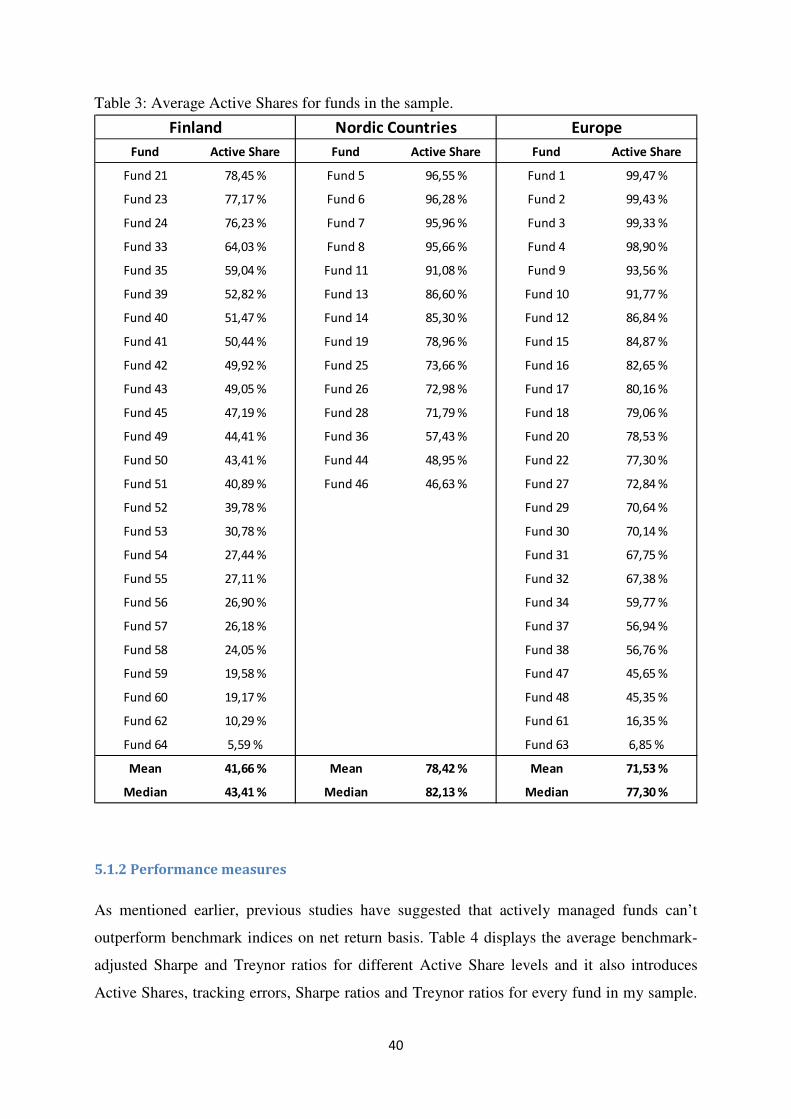
40

Table 3: Average Active Shares for funds in the sample.

5.1.2 Performance measures

As mentioned earlier, previous studies have suggested that actively managed funds can’t

outperform benchmark indices on net return basis. Table 4 displays the average benchmark-

adjusted Sharpe and Treynor ratios for different Active Share levels and it also introduces

Active Shares, tracking errors, Sharpe ratios and Treynor ratios for every fund in my sample.

Fund Active Share Fund Active Share Fund Active Share

Fund 21 78,45 % Fund 5 96,55 % Fund 1 99,47 %

Fund 23 77,17 % Fund 6 96,28 % Fund 2 99,43 %

Fund 24 76,23 % Fund 7 95,96 % Fund 3 99,33 %

Fund 33 64,03 % Fund 8 95,66 % Fund 4 98,90 %

Fund 35 59,04 % Fund 11 91,08 % Fund 9 93,56 %

Fund 39 52,82 % Fund 13 86,60 % Fund 10 91,77 %

Fund 40 51,47 % Fund 14 85,30 % Fund 12 86,84 %

Fund 41 50,44 % Fund 19 78,96 % Fund 15 84,87 %

Fund 42 49,92 % Fund 25 73,66 % Fund 16 82,65 %

Fund 43 49,05 % Fund 26 72,98 % Fund 17 80,16 %

Fund 45 47,19 % Fund 28 71,79 % Fund 18 79,06 %

Fund 49 44,41 % Fund 36 57,43 % Fund 20 78,53 %

Fund 50 43,41 % Fund 44 48,95 % Fund 22 77,30 %

Fund 51 40,89 % Fund 46 46,63 % Fund 27 72,84 %

Fund 52 39,78 % Fund 29 70,64 %

Fund 53 30,78 % Fund 30 70,14 %

Fund 54 27,44 % Fund 31 67,75 %

Fund 55 27,11 % Fund 32 67,38 %

Fund 56 26,90 % Fund 34 59,77 %

Fund 57 26,18 % Fund 37 56,94 %

Fund 58 24,05 % Fund 38 56,76 %

Fund 59 19,58 % Fund 47 45,65 %

Fund 60 19,17 % Fund 48 45,35 %

Fund 62 10,29 % Fund 61 16,35 %

Fund 64 5,59 % Fund 63 6,85 %

Mean 41,66 % Mean 78,42 % Mean 71,53 %

Median 43,41 % Median 82,13 % Median 77,30 %

Finland Nordic Countries Europe

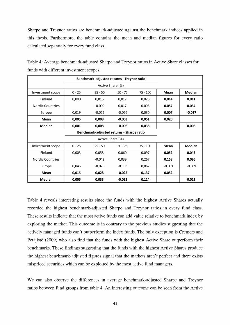
41

Sharpe and Treynor ratios are benchmark-adjusted against the benchmark indices applied in

this thesis. Furthermore, the table contains the mean and median figures for every ratio

calculated separately for every fund class.

Table 4: Average benchmark-adjusted Sharpe and Treynor ratios in Active Share classes for

funds with different investment scopes.

Table 4 reveals interesting results since the funds with the highest Active Shares actually

recorded the highest benchmark-adjusted Sharpe and Treynor ratios in every fund class.

These results indicate that the most active funds can add value relative to benchmark index by

exploring the market. This outcome is in contrary to the previous studies suggesting that the

actively managed funds can’t outperform the index funds. The only exception is Cremers and

Petäjistö (2009) who also find that the funds with the highest Active Share outperform their

benchmarks. These findings suggesting that the funds with the highest Active Shares produce

the highest benchmark-adjusted figures signal that the markets aren’t perfect and there exists

mispriced securities which can be exploited by the most active fund managers.

We can also observe the differences in average benchmark-adjusted Sharpe and Treynor

ratios between fund groups from table 4. An interesting outcome can be seen from the Active

Investment scope 0 - 25 25 - 50 50 - 75 75 - 100 Mean Median

Finland 0,000 0,016 0,017 0,026 0,014 0,011

Nordic Countries -0,009 0,017 0,093 0,057 0,034

Europe 0,019 -0,025 -0,026 0,030 0,007 -0,017

Mean 0,005 0,008 -0,003 0,051 0,020

Median 0,001 0,008 -0,006 0,038 0,008

Investment scope 0 - 25 25 - 50 50 - 75 75 - 100 Mean Median

Finland 0,003 0,058 0,060 0,097 0,052 0,043

Nordic Countries -0,042 0,039 0,267 0,158 0,096

Europe 0,045 -0,078 -0,103 0,067 -0,001 -0,069

Mean 0,015 0,028 -0,022 0,137 0,052

Median 0,005 0,033 -0,032 0,114 0,021

Benchmark-adjusted returns - Treynor ratio

Active Share (%)

Benchmark-adjusted returns - Sharpe ratio

Active Share (%)

42

Shares of the funds investing in Finland and Nordic Countries as the benchmark-adjusted

performance increases with the level of Active Share. The funds investing in Finland

outperformed the benchmark index in every Active Share levels and in the group of funds

investing in Nordic Countries only the most passive funds in the sample, in the Active Share

level of 25 – 50%, underperformed the benchmark index. From graph 1 we can see that

whereas the outperforming was more stable in the group of funds investing in Finland, the

benchmark-adjusted performance increased more sharply among the funds investing in

Nordic Countries as the Active Share increased. The funds investing in Europe beat the

benchmark index in the most active and passive Active Share levels whereas the benchmark

index performed better among the funds with Active Share between 25 – 75%.

Graph 1: Benchmark-adjusted Sharpe ratios in different Active Share levels.

Petäjistö (2010) find that the closet indexers can’t beat the benchmark indices and

underperform them after the fees. In my sample, as the table 4 shows, the closet indexers were

able to outperform the benchmark index in the class of funds investing in Finland whereas the

funds investing in Nordic Countries and Europe underperformed their benchmark indices.

Table 5 clearly shows that the equity funds investing in Finland have outperformed the OMX

Helsinki CAP GI Index on net return basis on the three-year period applied in this thesis. The

average Sharpe ratio for funds investing in Finland is 0,052 and Treynor ratio 0,014. The

-0,2

-0,1

0,0

0,1

0,2

0,3

0 - 25 25 - 50 50 - 75 75 - 100Sh

arp

e R

ati

o

Active Share (%)

Benchmark-adjusted Sharpe ratios in different Active Share levels

Finland Nordic Countries Europe Total

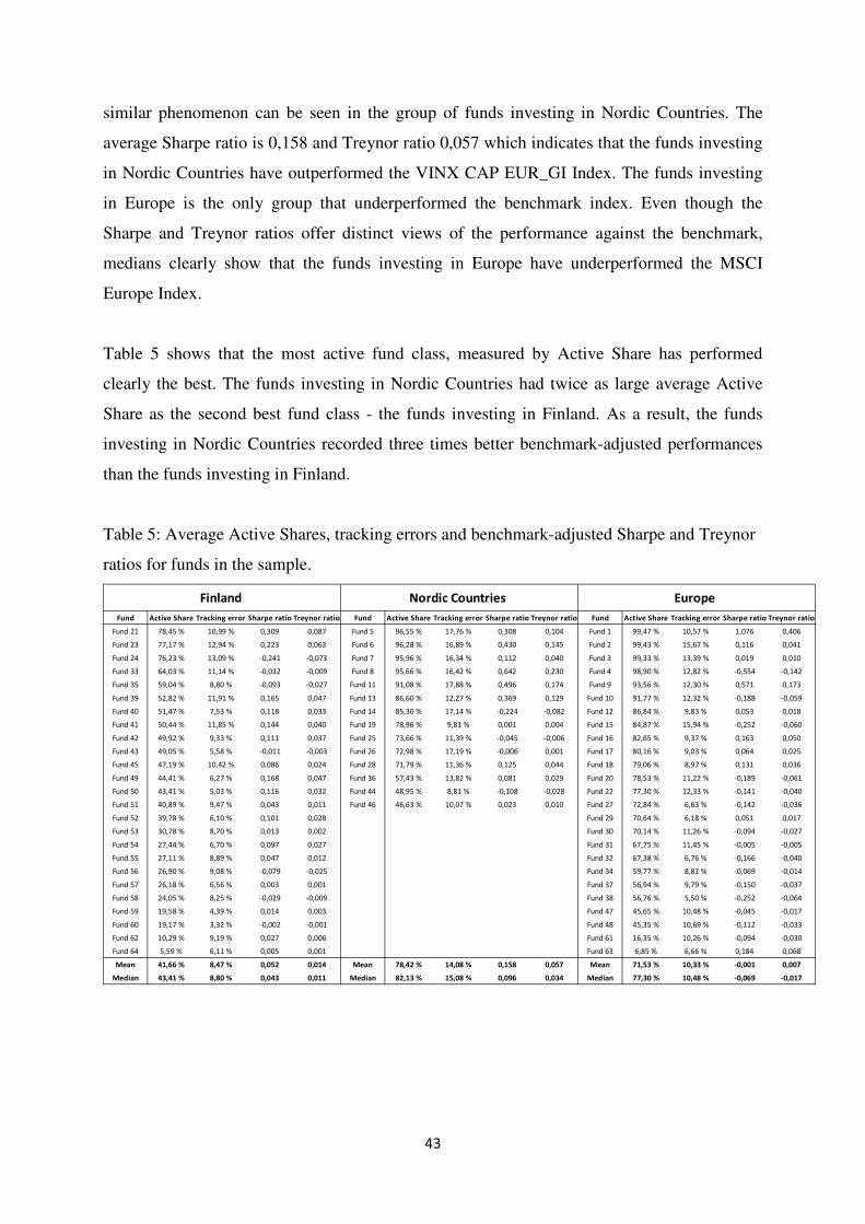
43

similar phenomenon can be seen in the group of funds investing in Nordic Countries. The

average Sharpe ratio is 0,158 and Treynor ratio 0,057 which indicates that the funds investing

in Nordic Countries have outperformed the VINX CAP EUR_GI Index. The funds investing

in Europe is the only group that underperformed the benchmark index. Even though the

Sharpe and Treynor ratios offer distinct views of the performance against the benchmark,

medians clearly show that the funds investing in Europe have underperformed the MSCI

Europe Index.

Table 5 shows that the most active fund class, measured by Active Share has performed

clearly the best. The funds investing in Nordic Countries had twice as large average Active

Share as the second best fund class - the funds investing in Finland. As a result, the funds

investing in Nordic Countries recorded three times better benchmark-adjusted performances

than the funds investing in Finland.

Table 5: Average Active Shares, tracking errors and benchmark-adjusted Sharpe and Treynor

ratios for funds in the sample.

Fund Active Share Tracking error Sharpe ratio Treynor ratio Fund Active Share Tracking error Sharpe ratio Treynor ratio Fund Active Share Tracking error Sharpe ratio Treynor ratio

Fund 21 78,45 % 10,99 % 0,309 0,087 Fund 5 96,55 % 17,76 % 0,308 0,104 Fund 1 99,47 % 10,57 % 1,076 0,406

Fund 23 77,17 % 12,94 % 0,223 0,063 Fund 6 96,28 % 16,89 % 0,430 0,145 Fund 2 99,43 % 15,67 % 0,116 0,041

Fund 24 76,23 % 13,09 % -0,241 -0,073 Fund 7 95,96 % 16,34 % 0,112 0,040 Fund 3 99,33 % 13,39 % 0,019 0,010

Fund 33 64,03 % 11,14 % -0,032 -0,009 Fund 8 95,66 % 16,42 % 0,642 0,230 Fund 4 98,90 % 12,82 % -0,554 -0,142

Fund 35 59,04 % 8,80 % -0,093 -0,027 Fund 11 91,08 % 17,88 % 0,496 0,174 Fund 9 93,56 % 12,30 % 0,571 0,173

Fund 39 52,82 % 11,91 % 0,165 0,047 Fund 13 86,60 % 12,27 % 0,369 0,129 Fund 10 91,77 % 12,32 % -0,188 -0,059

Fund 40 51,47 % 7,53 % 0,118 0,033 Fund 14 85,30 % 17,14 % -0,224 -0,082 Fund 12 86,84 % 9,83 % 0,053 0,018

Fund 41 50,44 % 11,85 % 0,144 0,040 Fund 19 78,96 % 9,81 % 0,001 0,004 Fund 15 84,87 % 15,94 % -0,252 -0,060

Fund 42 49,92 % 9,33 % 0,111 0,037 Fund 25 73,66 % 11,39 % -0,045 -0,006 Fund 16 82,65 % 9,37 % 0,163 0,050

Fund 43 49,05 % 5,58 % -0,011 -0,003 Fund 26 72,98 % 17,19 % -0,006 0,001 Fund 17 80,16 % 9,03 % 0,064 0,025

Fund 45 47,19 % 10,42 % 0,086 0,024 Fund 28 71,79 % 11,36 % 0,125 0,044 Fund 18 79,06 % 8,97 % 0,131 0,036

Fund 49 44,41 % 6,27 % 0,168 0,047 Fund 36 57,43 % 13,82 % 0,081 0,029 Fund 20 78,53 % 11,22 % -0,189 -0,061

Fund 50 43,41 % 5,03 % 0,116 0,032 Fund 44 48,95 % 8,81 % -0,108 -0,028 Fund 22 77,30 % 12,33 % -0,141 -0,040

Fund 51 40,89 % 9,47 % 0,043 0,011 Fund 46 46,63 % 10,07 % 0,023 0,010 Fund 27 72,84 % 6,63 % -0,142 -0,036

Fund 52 39,78 % 6,10 % 0,101 0,028 Fund 29 70,64 % 6,18 % 0,051 0,017

Fund 53 30,78 % 8,70 % 0,013 0,002 Fund 30 70,14 % 11,26 % -0,094 -0,027

Fund 54 27,44 % 6,70 % 0,097 0,027 Fund 31 67,75 % 11,45 % -0,005 -0,005

Fund 55 27,11 % 8,89 % 0,047 0,012 Fund 32 67,38 % 6,76 % -0,166 -0,040

Fund 56 26,90 % 9,08 % -0,079 -0,025 Fund 34 59,77 % 8,82 % -0,069 -0,014

Fund 57 26,18 % 6,56 % 0,003 0,001 Fund 37 56,94 % 9,79 % -0,150 -0,037

Fund 58 24,05 % 8,25 % -0,029 -0,009 Fund 38 56,76 % 5,50 % -0,252 -0,064

Fund 59 19,58 % 4,39 % 0,014 0,003 Fund 47 45,65 % 10,48 % -0,045 -0,017

Fund 60 19,17 % 3,32 % -0,002 -0,001 Fund 48 45,35 % 10,69 % -0,112 -0,033

Fund 62 10,29 % 9,19 % 0,027 0,006 Fund 61 16,35 % 10,26 % -0,094 -0,030

Fund 64 5,59 % 6,11 % 0,005 0,001 Fund 63 6,85 % 6,66 % 0,184 0,068

Mean 41,66 % 8,47 % 0,052 0,014 Mean 78,42 % 14,08 % 0,158 0,057 Mean 71,53 % 10,33 % -0,001 0,007

Median 43,41 % 8,80 % 0,043 0,011 Median 82,13 % 15,08 % 0,096 0,034 Median 77,30 % 10,48 % -0,069 -0,017

Finland Nordic Countries Europe

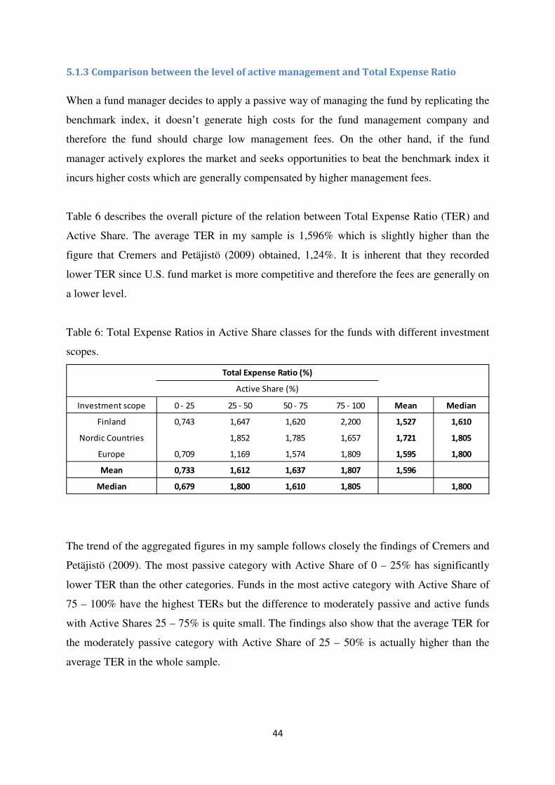
44

5.1.3 Comparison between the level of active management and Total Expense Ratio

When a fund manager decides to apply a passive way of managing the fund by replicating the

benchmark index, it doesn’t generate high costs for the fund management company and

therefore the fund should charge low management fees. On the other hand, if the fund

manager actively explores the market and seeks opportunities to beat the benchmark index it

incurs higher costs which are generally compensated by higher management fees.

Table 6 describes the overall picture of the relation between Total Expense Ratio (TER) and

Active Share. The average TER in my sample is 1,596% which is slightly higher than the

figure that Cremers and Petäjistö (2009) obtained, 1,24%. It is inherent that they recorded

lower TER since U.S. fund market is more competitive and therefore the fees are generally on

a lower level.

Table 6: Total Expense Ratios in Active Share classes for the funds with different investment

scopes.

The trend of the aggregated figures in my sample follows closely the findings of Cremers and

Petäjistö (2009). The most passive category with Active Share of 0 – 25% has significantly

lower TER than the other categories. Funds in the most active category with Active Share of

75 – 100% have the highest TERs but the difference to moderately passive and active funds

with Active Shares 25 – 75% is quite small. The findings also show that the average TER for

the moderately passive category with Active Share of 25 – 50% is actually higher than the

average TER in the whole sample.

Investment scope 0 - 25 25 - 50 50 - 75 75 - 100 Mean Median

Finland 0,743 1,647 1,620 2,200 1,527 1,610

Nordic Countries 1,852 1,785 1,657 1,721 1,805

Europe 0,709 1,169 1,574 1,809 1,595 1,800

Mean 0,733 1,612 1,637 1,807 1,596

Median 0,679 1,800 1,610 1,805 1,800

Active Share (%)

Total Expense Ratio (%)

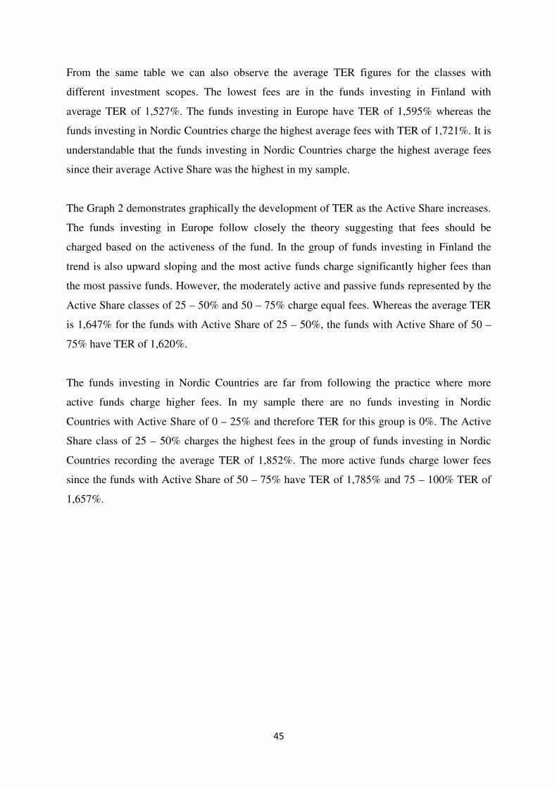
45

From the same table we can also observe the average TER figures for the classes with

different investment scopes. The lowest fees are in the funds investing in Finland with

average TER of 1,527%. The funds investing in Europe have TER of 1,595% whereas the

funds investing in Nordic Countries charge the highest average fees with TER of 1,721%. It is

understandable that the funds investing in Nordic Countries charge the highest average fees

since their average Active Share was the highest in my sample.

The Graph 2 demonstrates graphically the development of TER as the Active Share increases.

The funds investing in Europe follow closely the theory suggesting that fees should be

charged based on the activeness of the fund. In the group of funds investing in Finland the

trend is also upward sloping and the most active funds charge significantly higher fees than

the most passive funds. However, the moderately active and passive funds represented by the

Active Share classes of 25 – 50% and 50 – 75% charge equal fees. Whereas the average TER

is 1,647% for the funds with Active Share of 25 – 50%, the funds with Active Share of 50 –

75% have TER of 1,620%.

The funds investing in Nordic Countries are far from following the practice where more

active funds charge higher fees. In my sample there are no funds investing in Nordic

Countries with Active Share of 0 – 25% and therefore TER for this group is 0%. The Active

Share class of 25 – 50% charges the highest fees in the group of funds investing in Nordic

Countries recording the average TER of 1,852%. The more active funds charge lower fees

since the funds with Active Share of 50 – 75% have TER of 1,785% and 75 – 100% TER of

1,657%.

46

Graph 2: Total Expense Ratios in different Active Share levels.

It is reasonable that the funds investing in Finland charge the lowest fees. First, the Finnish

market is significantly smaller than the market of funds investing in Nordic Countries and

Europe and therefore Finnish market can be explored with smaller effort. Second, in my

sample the average Active Share of the funds investing in Finland was considerably lower

than on the funds investing Nordic Countries and Europe. Therefore the average fees also

need to be lower within the funds investing in Finland. Taking these things into account, the

average TER should actually be even lower for funds investing Finland compared to the

average level of TERs for funds investing in Nordic Countries and Europe.

Table 7 also provides us information about closet indexing. The funds with Active Share of

25 – 50% are moderately passive but they still charge high fees in every fund group.

Especially, the funds investing in Finland and Nordic Countries with TERs over 1,5% can’t

provide enough value relative to index funds to compensate their high fees. Therefore

investors would clearly be better off by investing in an index fund.

0,0

0,5

1,0

1,5

2,0

2,5

0 - 25 25 - 50 50 - 75 75 - 100

Tota

l E

xpe

nse

Ra

tio

(%

)

Active Share (%)

Total Expense Ratios in different Active Share levels

Finland Nordic Countries Europe

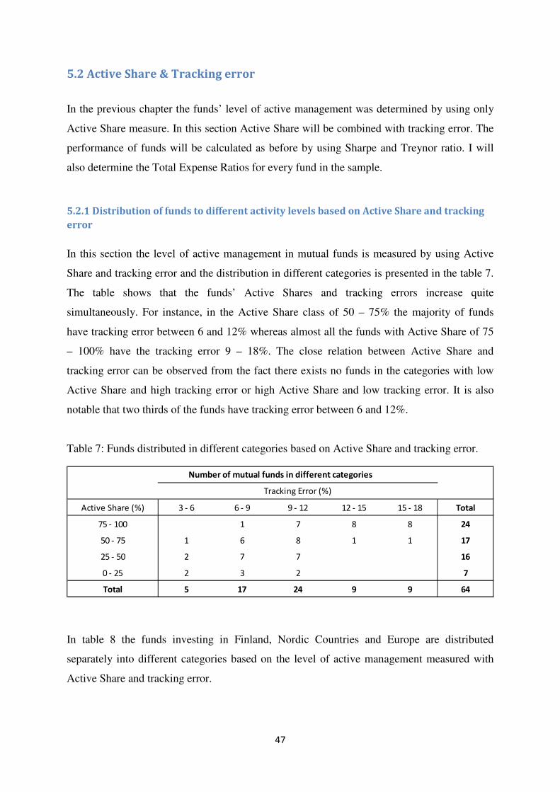
47

5.2 Active Share & Tracking error

In the previous chapter the funds’ level of active management was determined by using only

Active Share measure. In this section Active Share will be combined with tracking error. The

performance of funds will be calculated as before by using Sharpe and Treynor ratio. I will

also determine the Total Expense Ratios for every fund in the sample.

5.2.1 Distribution of funds to different activity levels based on Active Share and tracking

error

In this section the level of active management in mutual funds is measured by using Active

Share and tracking error and the distribution in different categories is presented in the table 7.

The table shows that the funds’ Active Shares and tracking errors increase quite

simultaneously. For instance, in the Active Share class of 50 – 75% the majority of funds

have tracking error between 6 and 12% whereas almost all the funds with Active Share of 75

– 100% have the tracking error 9 – 18%. The close relation between Active Share and

tracking error can be observed from the fact there exists no funds in the categories with low

Active Share and high tracking error or high Active Share and low tracking error. It is also

notable that two thirds of the funds have tracking error between 6 and 12%.

Table 7: Funds distributed in different categories based on Active Share and tracking error.

In table 8 the funds investing in Finland, Nordic Countries and Europe are distributed

separately into different categories based on the level of active management measured with

Active Share and tracking error.

Active Share (%) 3 - 6 6 - 9 9 - 12 12 - 15 15 - 18 Total

75 - 100 1 7 8 8 24

50 - 75 1 6 8 1 1 17

25 - 50 2 7 7 16

0 - 25 2 3 2 7

Total 5 17 24 9 9 64

Number of mutual funds in different categories

Tracking Error (%)

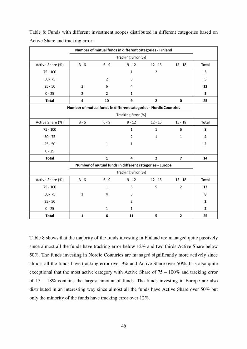
48

Table 8: Funds with different investment scopes distributed in different categories based on

Active Share and tracking error.

Table 8 shows that the majority of the funds investing in Finland are managed quite passively

since almost all the funds have tracking error below 12% and two thirds Active Share below

50%. The funds investing in Nordic Countries are managed significantly more actively since

almost all the funds have tracking error over 9% and Active Share over 50%. It is also quite

exceptional that the most active category with Active Share of 75 – 100% and tracking error

of 15 – 18% contains the largest amount of funds. The funds investing in Europe are also

distributed in an interesting way since almost all the funds have Active Share over 50% but

only the minority of the funds have tracking error over 12%.

Active Share (%) 3 - 6 6 - 9 9 - 12 12 - 15 15 - 18 Total

75 - 100 1 2 3

50 - 75 2 3 5

25 - 50 2 6 4 12

0 - 25 2 2 1 5

Total 4 10 9 2 0 25

Active Share (%) 3 - 6 6 - 9 9 - 12 12 - 15 15 - 18 Total

75 - 100 1 1 6 8

50 - 75 2 1 1 4

25 - 50 1 1 2

0 - 25

Total 1 4 2 7 14

Active Share (%) 3 - 6 6 - 9 9 - 12 12 - 15 15 - 18 Total

75 - 100 1 5 5 2 13

50 - 75 1 4 3 8

25 - 50 2 2

0 - 25 1 1 2

Total 1 6 11 5 2 25

Tracking Error (%)

Number of mutual funds in different categories - Finland

Tracking Error (%)

Number of mutual funds in different categories - Nordic Countries

Tracking Error (%)

Number of mutual funds in different categories - Europe

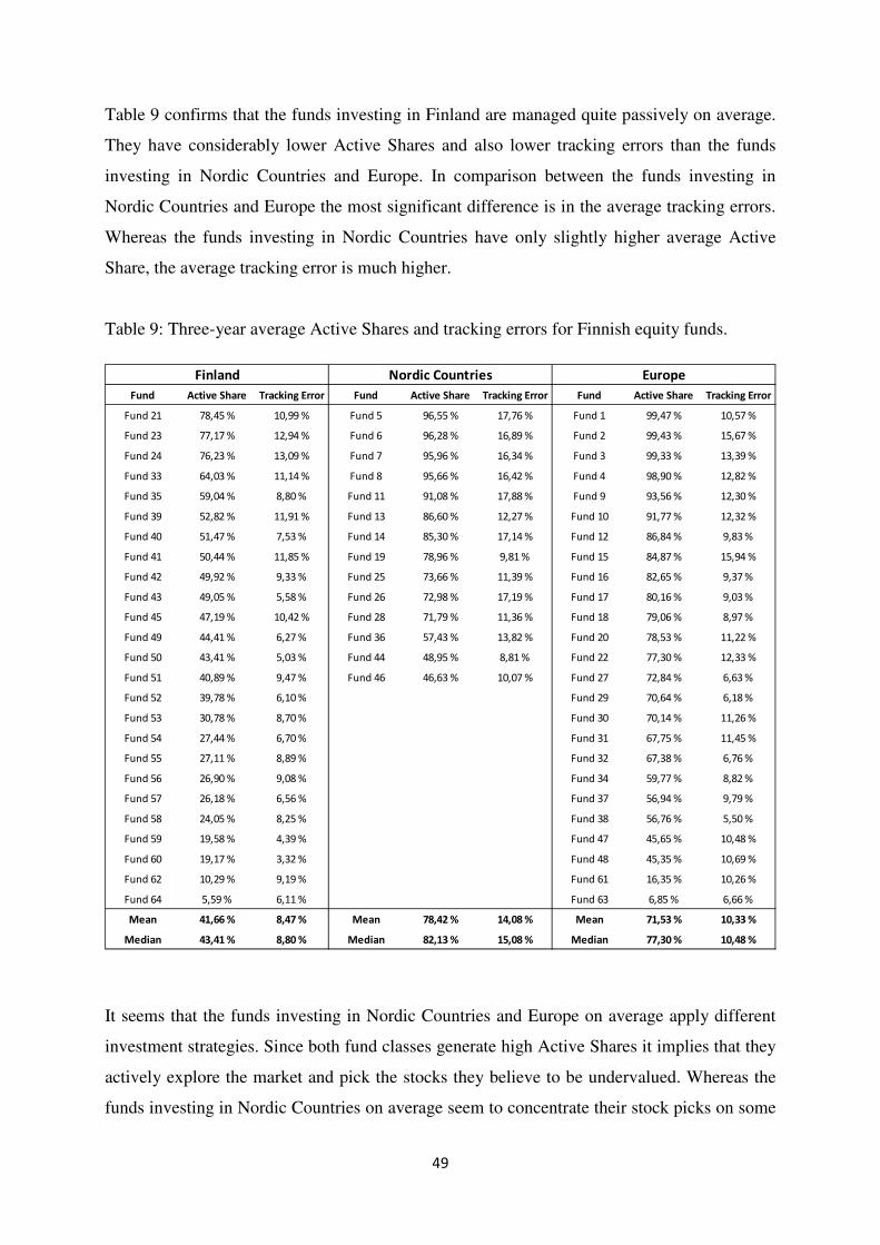
49

Table 9 confirms that the funds investing in Finland are managed quite passively on average.

They have considerably lower Active Shares and also lower tracking errors than the funds

investing in Nordic Countries and Europe. In comparison between the funds investing in

Nordic Countries and Europe the most significant difference is in the average tracking errors.

Whereas the funds investing in Nordic Countries have only slightly higher average Active

Share, the average tracking error is much higher.

Table 9: Three-year average Active Shares and tracking errors for Finnish equity funds.

It seems that the funds investing in Nordic Countries and Europe on average apply different

investment strategies. Since both fund classes generate high Active Shares it implies that they

actively explore the market and pick the stocks they believe to be undervalued. Whereas the

funds investing in Nordic Countries on average seem to concentrate their stock picks on some

Fund Active Share Tracking Error Fund Active Share Tracking Error Fund Active Share Tracking Error

Fund 21 78,45 % 10,99 % Fund 5 96,55 % 17,76 % Fund 1 99,47 % 10,57 %

Fund 23 77,17 % 12,94 % Fund 6 96,28 % 16,89 % Fund 2 99,43 % 15,67 %

Fund 24 76,23 % 13,09 % Fund 7 95,96 % 16,34 % Fund 3 99,33 % 13,39 %

Fund 33 64,03 % 11,14 % Fund 8 95,66 % 16,42 % Fund 4 98,90 % 12,82 %

Fund 35 59,04 % 8,80 % Fund 11 91,08 % 17,88 % Fund 9 93,56 % 12,30 %

Fund 39 52,82 % 11,91 % Fund 13 86,60 % 12,27 % Fund 10 91,77 % 12,32 %

Fund 40 51,47 % 7,53 % Fund 14 85,30 % 17,14 % Fund 12 86,84 % 9,83 %

Fund 41 50,44 % 11,85 % Fund 19 78,96 % 9,81 % Fund 15 84,87 % 15,94 %

Fund 42 49,92 % 9,33 % Fund 25 73,66 % 11,39 % Fund 16 82,65 % 9,37 %

Fund 43 49,05 % 5,58 % Fund 26 72,98 % 17,19 % Fund 17 80,16 % 9,03 %

Fund 45 47,19 % 10,42 % Fund 28 71,79 % 11,36 % Fund 18 79,06 % 8,97 %

Fund 49 44,41 % 6,27 % Fund 36 57,43 % 13,82 % Fund 20 78,53 % 11,22 %

Fund 50 43,41 % 5,03 % Fund 44 48,95 % 8,81 % Fund 22 77,30 % 12,33 %

Fund 51 40,89 % 9,47 % Fund 46 46,63 % 10,07 % Fund 27 72,84 % 6,63 %

Fund 52 39,78 % 6,10 % Fund 29 70,64 % 6,18 %

Fund 53 30,78 % 8,70 % Fund 30 70,14 % 11,26 %

Fund 54 27,44 % 6,70 % Fund 31 67,75 % 11,45 %

Fund 55 27,11 % 8,89 % Fund 32 67,38 % 6,76 %

Fund 56 26,90 % 9,08 % Fund 34 59,77 % 8,82 %

Fund 57 26,18 % 6,56 % Fund 37 56,94 % 9,79 %

Fund 58 24,05 % 8,25 % Fund 38 56,76 % 5,50 %

Fund 59 19,58 % 4,39 % Fund 47 45,65 % 10,48 %

Fund 60 19,17 % 3,32 % Fund 48 45,35 % 10,69 %

Fund 62 10,29 % 9,19 % Fund 61 16,35 % 10,26 %

Fund 64 5,59 % 6,11 % Fund 63 6,85 % 6,66 %

Mean 41,66 % 8,47 % Mean 78,42 % 14,08 % Mean 71,53 % 10,33 %

Median 43,41 % 8,80 % Median 82,13 % 15,08 % Median 77,30 % 10,48 %

EuropeFinland Nordic Countries

50

specific industries generating high tracking error, the funds investing in Europe diversify their

stock picks on all industries generating lower tracking error.

5.2.2 Performance measures

Table 10 introduces very interesting results concerning the benchmark-adjusted returns for the

sample. The most active levels of both Active Share and tracking error produce the highest

returns. The Active Share level of 75 – 100% has mean Sharpe of 0,137 and Treynor ratio of

0,051 whereas the second best level is Active Share of 25 – 50% with Sharpe ratio of 0,028

and Treynor ratio of 0,008. The tracking error of 15 – 18% has mean Sharpe ratio of 0,180

and Treynor ratio of 0,066 while the second best level produces Sharpe ratio of 0,064 and

Treynor ratio 0,023. These findings are similar with the results of Cremers and Petäjistö

(2009). The most active funds appear to have stock-picking ability which enables them to

outperform the benchmark indices even after fees.

Table 10: Average benchmark-adjusted Sharpe and Treynor ratios in different categories

based on Active Share and tracking error.

Active Share (%) 3 - 6 6 - 9 9 - 12 12 - 15 15 - 18 Mean Median

75 - 100 0,036 0,076 0,008 0,074 0,051 0,038

50 - 75 -0,064 -0,011 0,006 0,029 0,001 -0,003 -0,006

25 - 50 0,015 0,013 0,001 0,008 0,008

0 - 25 0,001 0,000 -0,012 -0,003 0,001

Mean -0,007 0,003 0,023 0,010 0,066 0,020

Median -0,001 0,002 0,008 0,010 0,041 0,008

Active Share (%) 3 - 6 6 - 9 9 - 12 12 - 15 15 - 18 Mean Median

75 - 100 0,131 0,211 0,007 0,204 0,137 0,114

50 - 75 -0,252 -0,050 0,014 0,081 -0,006 -0,022 -0,032

25 - 50 0,052 0,046 0,004 0,028 0,033

0 - 25 0,006 0,007 -0,034 -0,005 0,005

Mean -0,027 0,010 0,064 0,015 0,180 0,052

Median -0,002 0,013 0,025 0,019 0,116 0,021

Benchmark-adjusted returns - Sharpe ratio

Tracking Error (%)

Benchmark-adjusted returns - Treynor ratio

Tracking Error (%)

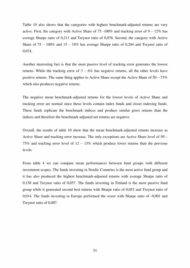
51

Table 10 also shows that the categories with highest benchmark-adjusted returns are very

active. First, the category with Active Share of 75 -100% and tracking error of 9 – 12% has

average Sharpe ratio of 0,211 and Treynor ratio of 0,076. Second, the category with Active

Share of 75 – 100% and 15 – 18% has average Sharpe ratio of 0,204 and Treynor ratio of

0,074.

Another interesting fact is that the most passive level of tracking error generates the lowest

returns. While the tracking error of 3 – 6% has negative returns, all the other levels have

positive returns. The same thing applies to Active Share except the Active Share of 50 – 75%

which also produces negative returns.

The negative mean benchmark-adjusted returns for the lowest levels of Active Share and

tracking error are normal since these levels contain index funds and closet indexing funds.

These funds replicate the benchmark indices and produce similar gross returns than the

indices and therefore the benchmark-adjusted net returns are negative.

Overall, the results of table 10 show that the mean benchmark-adjusted returns increase as

Active Share and tracking error increase. The only exceptions are Active Share level of 50 –

75% and tracking error level of 12 – 15% which produce lower returns than the previous

levels.

From table 4 we can compare mean performances between fund groups with different

investment scopes. The funds investing in Nordic Countries is the most active fund group and

it has also produced the highest benchmark-adjusted returns with average Sharpe ratio of

0,158 and Treynor ratio of 0,057. The funds investing in Finland is the most passive fund

group while it generated second best returns with Sharpe ratio of 0,052 and Treynor ratio of

0,014. The funds investing in Europe performed the worst with Sharpe ratio of -0,001 and

Treynor ratio of 0,007.

52

5.2.3 Comparison between the level of active management and Total Expense Ratio

Table 11 presents the average Total Expense Ratios for every activity categories based on

Active Share and tracking error. When exploring the mean figures of both Active Share and

tracking error it is easy to see that the sample funds follow on average the practice that higher

fees are charged by more actively managed funds. As tracking error increases the mean TER

also increases. The only exception is the highest tracking error class where the mean TER is

slightly smaller than in the tracking error class of 12 – 15%. The mean TER also increases

constantly as the average Active Share increases. The trend of TER increasing with Active

Share and tracking error follows closely the findings of Cremers and Petäjistö (2009).

Table 11: Average Total Expense Ratios in different categories based on Active Share and

tracking error.

The category with Active Share of 0 – 25% and tracking error of 3 – 6% has a mean TER of

0,332% which is very low. The reason is that the funds with the lowest Active Share and

tracking error are generally index funds which replicate benchmark indices and therefore

charge low fees. From the table 11 we can see that the categories close to the most passive

category charge significantly higher fees. Excluding the most passive category, the other

categories with Active Share below 50% and tracking error below 9% have mean TERs over

1% and from these categories the ones with Active Share of 25 – 50% have mean TERs even

over 1,5%.

These funds that are distributed to the categories close to the most passive category are closet

indexers. The funds’ holdings replicate the benchmark holdings by over 50% and funds’ daily

prices follow closely the movements of the benchmark indices. Consequently, the fund

Active Share (%) 3 - 6 6 - 9 9 - 12 12 - 15 15 - 18 Mean Median

75 - 100 1,700 1,713 2,017 1,694 1,807 1,805

50 - 75 1,862 1,392 1,744 1,860 1,810 1,637 1,610

25 - 50 1,790 1,566 1,608 1,612 1,800

0 - 25 0,332 1,111 0,567 0,733 0,679

Mean 1,221 1,432 1,597 1,999 1,707 1,596

Median 1,500 1,600 1,610 1,869 1,800 1,800

Total Expense Ratio (%)

Tracking Error (%)

53

managers aren’t actively taking bets in order to outperform the benchmark indices and

therefore the fees charged are too high. The investors would be better off by investing in an

index fund which replicates the benchmark index with considerably lower fees.

Table 12 describes how Total Expense Ratio varies with Active Share and tracking error

among different fund groups. The funds investing in Finland charge higher fees as the

activeness of the funds increase. The mean TER is larger as the Active Share and tracking

error increase and the most passive funds have the lowest mean TER whereas the most

actively managed funds charge the highest fees.

Table 12: Average Total Expense Ratios for funds with different investment scopes

distributed in categories based on Active Share and tracking error.

Active Share (%) 3 - 6 6 - 9 9 - 12 12 - 15 15 - 18 Mean Median

75 - 100 2,100 2,250 2,200 2,100

50 - 75 1,450 1,733 1,620 1,600

25 - 50 1,790 1,476 1,830 1,647 1,800

0 - 25 0,332 1,297 0,454 0,743 0,500

Mean 1,061 1,435 1,675 2,250 1,527

Median 1,000 1,555 1,830 2,250 1,610

Active Share (%) 3 - 6 6 - 9 9 - 12 12 - 15 15 - 18 Mean Median

75 - 100 1,500 1,855 1,650 1,657 1,700

50 - 75 1,735 1,860 1,810 1,785 1,835

25 - 50 2,104 1,600 1,852 1,852

0 - 25

Mean 2,104 1,642 1,858 1,673 1,721

Median 2,104 1,600 1,858 1,800 1,805

Active Share (%) 3 - 6 6 - 9 9 - 12 12 - 15 15 - 18 Mean Median

75 - 100 1,700 1,678 1,956 1,825 1,809 1,800

50 - 75 1,862 1,363 1,760 1,574 1,705

25 - 50 1,169 1,169 1,169

0 - 25 0,740 0,679 0,709 0,709

Mean 1,862 1,315 1,517 1,956 1,825 1,595

Median 1,862 1,450 1,610 1,869 1,825 1,800

Total Expense Ratio (%) - Finland

Tracking Error (%)

Total Expense Ratio (%) - Nordic Countries

Tracking Error (%)

Total Expense Ratio (%) - Europe

Tracking Error (%)

54

The funds investing in Nordic Countries produced very unusual results. The average TER in

every category is between 1,5% and 2,1% but there is no correlation between the fees and the

level of active management. Whereas the most active funds have the highest fees among the

funds investing in Finland, the most passive category with Active Share of 25 – 50% and

tracking error of 6 – 9% charged the highest fees within the funds investing in Nordic

Countries.

When observing Active Share the funds investing in Europe charge higher fees as the level of

Active Share increases. The most passive funds have very low mean TER and expenses

increase steadily with the level of activity. However, the situation is more complex with

tracking error. In terms of tracking error, funds in the most passive category charge very high

fees. When excluding the most passive category, the mean TER increases with the level of

tracking error.

The average TER for closet indexing funds is 1,49% which is almost the same as the average

of the whole sample used in this thesis. When studying the fund groups separately we can see

that there are differences in closet indexing between funds with different investment scopes.

The group of funds investing in Finland contains the most of the closet indexing funds. 10

funds of the total 25 funds can be considered as closet indexing funds and the average TER

for these funds is 1,50%. The funds investing in Nordic Countries and Europe both contain

only 1 closet indexing fund. The fund investing in Europe has TER only 0,74% whereas the

fund investing in Nordic Countries charged 2,10%.

55

6 Conclusions

This thesis studies the active management in Finnish equity funds investing in Finland,

Nordic Countries and Europe. The time period applied in this thesis is from the first quarter of

2008 to the third quarter of 2010 in which the funds are analyzed with Active Share and

tracking error activities.

Active Share (Cremers and Petäjistö, 2006) is a rather new method for measuring fund’s

activity relative to is benchmark index. The basic idea of Active Share is to determine the

amount of active management by measuring how closely the holdings of the fund replicate the

holdings of the benchmark index. Active Share describes the percentage of stock holdings in a

fund that differ from those in the index. The more the fund deviates from the index, the more

active the fund is. Tracking error is a more traditional method and it measures how closely the

fund’s daily prices follow the prices of the benchmark index.

The average Active Share for the funds in my sample is 61,37%. The most active class with

Active Share of 75 – 100% contains the largest amount of funds representing the 37,5% of the

funds and 64,1% of the funds have Active Share over 50%. The average tracking error is

10,42% and 28,1% of the funds have tracking error over 12%. These figures mean that a little

less than 40% of the funds’ assets are on average invested in accordance with the benchmark

indices and over one fourth of the funds in the sample have substantially different daily

movements than the benchmark indices.

Cremers and Petäjistö (2006) discovered in their research in the U.S. that about 16,6 percent

of their sample funds had Active Share below 50%. There is a significant difference when

compared to my findings since in my sample 35,9% of the funds have Active Share below

50%. The reason can be found in the average Active Share figures between funds with

different investment scopes. The funds investing in Nordic Countries and Europe have

average Active Shares 14,3 percent and 16,0 percent respectively whereas the same figure for

the funds investing in Finland is 68,0 percent.

The same phenomenon can be found in the average Active Share figures. Whereas the funds

investing in Nordic Countries and Europe have average Active Share of 78,42% and 71,53%

respectively, the funds investing in Finland have substantially lower average figure with

56

41,66%. The same trend can be found from the average tracking errors. The funds investing in

Finland have the lowest tracking errors of 8,47% on average while the average tracking error

for the funds investing in Nordic Countries is 14,08% and in Europe 10,33%.

The equity funds investing in Finland follow the benchmark index much more frequently than

for example the funds in U.S. because the Finnish benchmark index contains a significantly

lower amount of stocks than the indices in U.S. Consequently, it is much easier and cheaper

to replicate the Finnish indices than the U.S. indices. Inversely put, there are significantly less

stocks available in Finland than in U.S. and therefore there are fewer options available for

fund managers while trying to outperform the benchmark index.

Compared to the funds investing in Finland, the funds investing in Nordic Countries and

Europe explore the market more intensively and take active positions more frequently

generating higher average Active Share and tracking error figures.

The fund distribution in my study shows the similar outcome than Cremers and Petäjistö

(2009) in the U.S; there are plenty of closet indexing funds in the Finnish equity fund market.

12 funds out of 64 funds fit inside the boundaries of “index funds” used in this thesis. The

worst part is that these funds also charge substantial fees compared to their activity levels.

The average TER for closet indexing funds is 1,49% which is almost the same as the average

of the whole sample used in this thesis.

When studying the fund groups separately we can see that there are differences in closet

indexing between funds with different investment scopes. The group of funds investing in

Finland contains the most of the closet indexing funds. 10 funds of the total 25 funds can be

considered as closet indexing funds and the average TER for these funds is substantially

large, 1,50%. The funds investing in Nordic Countries and Europe both contain only 1 closet

indexing fund. The fund investing in Europe has TER only 0,74% whereas the fund investing

in Nordic Countries charged 2,10%.

When observing the Total Expense Ratios for the whole sample, we can see that the trend in

Finnish equity markets follows closely the findings of Cremers and Petäjistö (2009) in the

U.S. markets; the average TER increases with the level of active management. There are few

57

exceptions, for example the relatively high TERs of the closet indexing funds, but the general

rule is that the level of active management and TER has a strong connection.

The funds investing in Finland have the lowest average Total Expense Ratios. This is

reasonable since these funds are substantially more passive than the funds investing in Nordic

Countries and Europe. Another reason for low fees is that the Finnish market is significantly

smaller than the ones of Nordic Countries and Europe and therefore Finnish market can be

explored with smaller effort. The funds investing in Nordic Countries have the highest

average Total Expense Ratios. It is also understandable since these funds are on average the

most actively managed.

My thesis has two main outcomes concerning the performance of the funds. First, the level of

performance increases the level of active management increases. Second, the most actively

managed funds have the best performances. These findings are in contradiction with the vast

majority of the previous studies (see e.g. Hendricks, Patel & Zeckhauser, 1993 and Blake &

Timmermann, 1998) suggesting that actively managed funds can’t outperform benchmark

indices on net return basis. However, my findings are similar with the results of Cremers and

Petäjistö (2009) who applied Active Share in determining the funds’ levels of active

management.

The most active funds appear to have stock-picking ability which enables them to outperform

the benchmark indices even after fees. These results indicate that the most active funds can

add value relative to benchmark index by exploring the market. This outcome is in contrary to

the previous studies suggesting that the actively managed funds can’t outperform the index

funds. The only exception is Cremers and Petäjistö (2009) who also find that the funds with

the highest Active Share outperform their benchmarks. These findings suggesting that the

funds with the highest Active Shares produce the highest benchmark-adjusted figures signal

that the markets aren’t perfect and there exists mispriced securities which can be exploited by

the most active fund managers.

On average, the funds investing in Finland and Nordic Countries were able to beat the

benchmark indices whereas the funds investing in Europe produced quite similar returns as

the benchmark. We can conclude that the European fund market is working more efficiently

than the Finnish market and the market of Nordic Countries since the fund managers investing

58

in European market haven’t been able to beat the benchmark index. At the same time the fund

managers investing in Finland and Nordic Countries have found inefficiencies in the markets

and outperformed the benchmark indices by exploiting these inefficiencies. Since the

European fund market is considerably larger and more competitive than these other markets,

it is reasonable that the fund managers have beaten the benchmark indices in the Finnish

market and the market of Nordic Countries.

It is also noteworthy that the most actively managed funds have the best performances among

every fund group with different investment scopes. Therefore we can say that the most

actively managed funds can find profitable investment opportunities from every market

included in this thesis. Even though European market can be considered to be highly

competitive, the intensive exploration of the market still pays off with higher after fees returns

than the benchmark index.

When thinking about the generalizability of the above discussed findings, there are some

limitations relating to them. First, the sample period is relatively short and a longer time

horizon would give us a more comprehensive view of the situation in different economic

conditions. Second, the sample in this thesis includes 64 funds which might restrict to

generalize the findings from the Finnish mutual fund market. Third, the holdings data used in

this thesis, describes the situations of funds and benchmarks on a quarterly basis. It would be

more informative if the holdings data would be available on a daily basis. Fourth, data

restrictions are also posed by the availability of the benchmark data which is why I have used

only one benchmark index against each fund in the sample. Additional benchmarks could give

more precise information about the funds’ movements towards the indices. Due to these facts,

the results of this thesis should be interpreted with some caution.

Based on this thesis, there are few suggestions for further research. First, the data used could

be extended to include larger amount of funds and longer time horizon. This way the findings

could be generalized with greater certainty. Second, the study could be included with new

fund groups i.e. funds with different investment scopes. It would be interesting to see how the

findings vary between several fund groups.

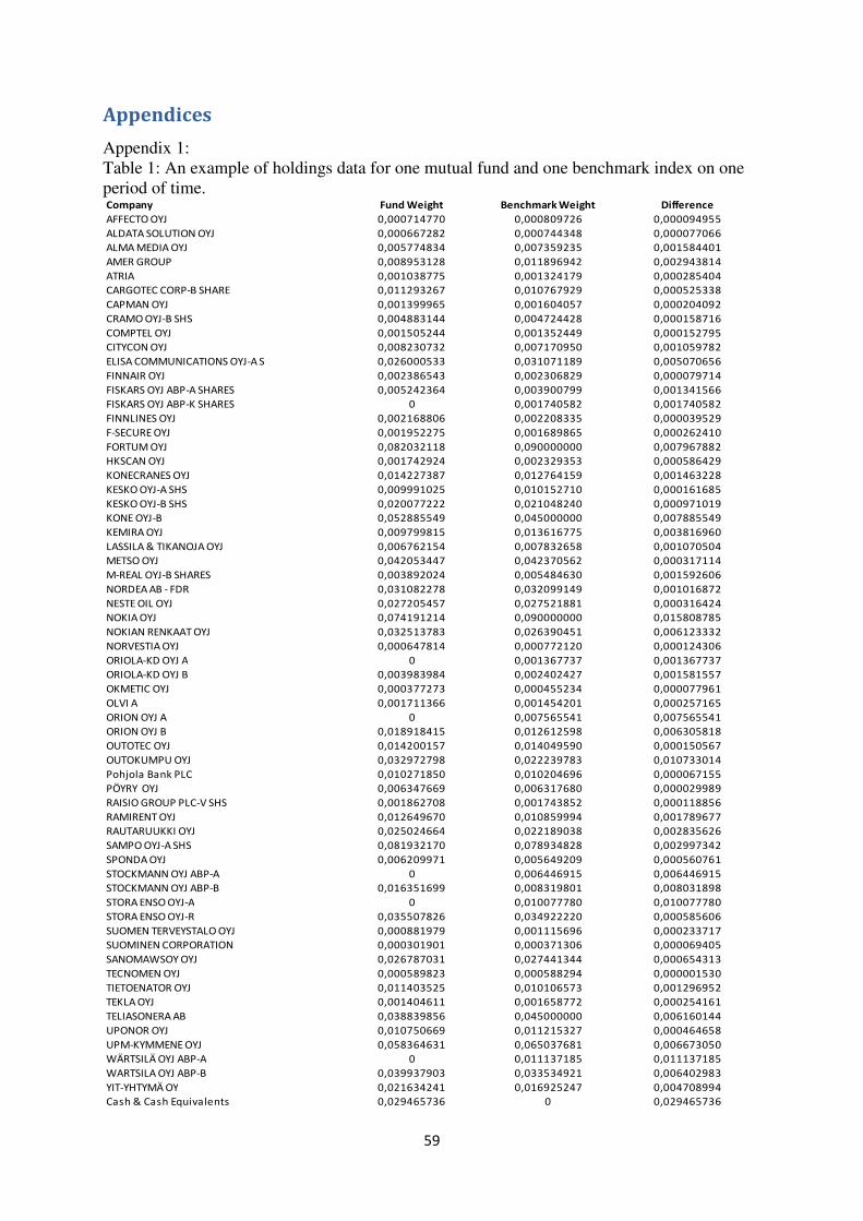
59

Appendices

Appendix 1:

Table 1: An example of holdings data for one mutual fund and one benchmark index on one

period of time.

Company Fund Weight Benchmark Weight Difference

AFFECTO OYJ 0,000714770 0,000809726 0,000094955

ALDATA SOLUTION OYJ 0,000667282 0,000744348 0,000077066

ALMA MEDIA OYJ 0,005774834 0,007359235 0,001584401

AMER GROUP 0,008953128 0,011896942 0,002943814

ATRIA 0,001038775 0,001324179 0,000285404

CARGOTEC CORP-B SHARE 0,011293267 0,010767929 0,000525338

CAPMAN OYJ 0,001399965 0,001604057 0,000204092

CRAMO OYJ-B SHS 0,004883144 0,004724428 0,000158716

COMPTEL OYJ 0,001505244 0,001352449 0,000152795

CITYCON OYJ 0,008230732 0,007170950 0,001059782

ELISA COMMUNICATIONS OYJ-A S 0,026000533 0,031071189 0,005070656

FINNAIR OYJ 0,002386543 0,002306829 0,000079714

FISKARS OYJ ABP-A SHARES 0,005242364 0,003900799 0,001341566

FISKARS OYJ ABP-K SHARES 0 0,001740582 0,001740582

FINNLINES OYJ 0,002168806 0,002208335 0,000039529

F-SECURE OYJ 0,001952275 0,001689865 0,000262410

FORTUM OYJ 0,082032118 0,090000000 0,007967882

HKSCAN OYJ 0,001742924 0,002329353 0,000586429

KONECRANES OYJ 0,014227387 0,012764159 0,001463228

KESKO OYJ-A SHS 0,009991025 0,010152710 0,000161685

KESKO OYJ-B SHS 0,020077222 0,021048240 0,000971019

KONE OYJ-B 0,052885549 0,045000000 0,007885549

KEMIRA OYJ 0,009799815 0,013616775 0,003816960

LASSILA & TIKANOJA OYJ 0,006762154 0,007832658 0,001070504

METSO OYJ 0,042053447 0,042370562 0,000317114

M-REAL OYJ-B SHARES 0,003892024 0,005484630 0,001592606

NORDEA AB - FDR 0,031082278 0,032099149 0,001016872

NESTE OIL OYJ 0,027205457 0,027521881 0,000316424

NOKIA OYJ 0,074191214 0,090000000 0,015808785

NOKIAN RENKAAT OYJ 0,032513783 0,026390451 0,006123332

NORVESTIA OYJ 0,000647814 0,000772120 0,000124306

ORIOLA-KD OYJ A 0 0,001367737 0,001367737

ORIOLA-KD OYJ B 0,003983984 0,002402427 0,001581557

OKMETIC OYJ 0,000377273 0,000455234 0,000077961

OLVI A 0,001711366 0,001454201 0,000257165

ORION OYJ A 0 0,007565541 0,007565541

ORION OYJ B 0,018918415 0,012612598 0,006305818

OUTOTEC OYJ 0,014200157 0,014049590 0,000150567

OUTOKUMPU OYJ 0,032972798 0,022239783 0,010733014

Pohjola Bank PLC 0,010271850 0,010204696 0,000067155

PÖYRY OYJ 0,006347669 0,006317680 0,000029989

RAISIO GROUP PLC-V SHS 0,001862708 0,001743852 0,000118856

RAMIRENT OYJ 0,012649670 0,010859994 0,001789677

RAUTARUUKKI OYJ 0,025024664 0,022189038 0,002835626

SAMPO OYJ-A SHS 0,081932170 0,078934828 0,002997342

SPONDA OYJ 0,006209971 0,005649209 0,000560761

STOCKMANN OYJ ABP-A 0 0,006446915 0,006446915

STOCKMANN OYJ ABP-B 0,016351699 0,008319801 0,008031898

STORA ENSO OYJ-A 0 0,010077780 0,010077780

STORA ENSO OYJ-R 0,035507826 0,034922220 0,000585606

SUOMEN TERVEYSTALO OYJ 0,000881979 0,001115696 0,000233717

SUOMINEN CORPORATION 0,000301901 0,000371306 0,000069405

SANOMAWSOY OYJ 0,026787031 0,027441344 0,000654313

TECNOMEN OYJ 0,000589823 0,000588294 0,000001530

TIETOENATOR OYJ 0,011403525 0,010106573 0,001296952

TEKLA OYJ 0,001404611 0,001658772 0,000254161

TELIASONERA AB 0,038839856 0,045000000 0,006160144

UPONOR OYJ 0,010750669 0,011215327 0,000464658

UPM-KYMMENE OYJ 0,058364631 0,065037681 0,006673050

WÄRTSILÄ OYJ ABP-A 0 0,011137185 0,011137185

WARTSILA OYJ ABP-B 0,039937903 0,033534921 0,006402983

YIT-YHTYMÄ OY 0,021634241 0,016925247 0,004708994

Cash & Cash Equivalents 0,029465736 0 0,029465736

60

References

Ammann, M. and Tobler, J. (2000): Measurement and Decomposition of Tracking Error

Variance. Working Paper, Swiss Institute of Banking and Finance / University of St. Gallen.

Blake, D. and Timmermann, A. (1998): Mutual Fund Performance: Evidence from the U.K.

European Finance Review, Vol. 2, No. 1, 57-77.

Bodie, Z., Kane, A. and Marcus A. (2005): Investments, 6th

edition. McGraw-Hill, New York.

Campbell, J. and Shiller, R. (1988): The Dividend-Price Ratio and Expectations of Future

Dividends and Discount Factors. Review of Financial Studies, Vol. 1, No. 3, 195-228.

Carhart, M. (1997): On Persistence in Mutual Fund Performance. Journal of Finance, Vol. 52,

No. 1, 57-82.

Chiang, W. (1998): Optimizing Performance. Indexing for Maximum Investment Results. CP

Co. Publisher, Chicago.

Cremers, M. and Petäjistö, A. (2006): Active and Passive Positions by Mutual Funds.

Working Paper, Yale School of Management.

Cremers M. and Petäjistö A. (2009): How Active Is Your Fund Manager? A New Measure

That Predicts Performance. Review of Financial Studies, Vol. 22, No. 9, 3329-3365.

Davis, J. (2001): Mutual Fund Performance and Manager Style. Financial Analyst Journal,

Vol. 57, No. 1, 19-26.

Dreman D. and Berry M. (1995): Overreaction, Underreaction, and the Low-P/E Effect.

Financial Analysts Journal, Vol. 51, No. 4, 21–30.

Ehlern, S. (1997): International Private Banking: A Study on International Private Banking

with Special Focus on the Portfolio Management Business. Verlag Paul Haupt, Bern;

Stuttgart; Wien.

Elton, E., Gruber, M. and Padberg M. (1976): Simple Criteria for Optimal Portfolio Selection.

Journal of Finance, Vol. 31, No. 5, 1341-1357.

Elton, E. and Gruber, M. (1999): Investments. The MIT Press, Cambridge.

61

Elton, E. and Gruber, M. (2003): Modern Portfolio Theory and Investment Analysis, 6th

edition. John Wiley & Sons, New York.

Elton, E., Gruber, M. and Blake, C. (1993): The Persistence of Risk-Adjusted Mutual Fund

Performance. Journal of Business, Vol. 69, No. 2, 133-157.

Elton, E. and Gruber, M. (1997): Modern Portfolio Theory, 1950 to Date. Journal of Banking

and Finance, Vol. 21, No. 11-12, 1743-1759.

Elton, E. and Gruber, M. (1974): Portfolio Theory When Investment Relatives Are

Lognormally Distributed. Journal of Finance, Vol. 29, No. 4, 1265-1273.

Elton, E., Gruber M. and Blake C. (1999): Common Factors in Active and Passive Portfolios.

European Financial Review, Vol. 3, No. 1, 53-78.

Fama, E. (1965): Portfolio Analysis in the Stable Paretian Market. Management Science, Vol.

11, No. 3, 404-419.

Fama, E. (1970a): Efficient Capital Markets: A Review of Theory and Empirical Work.

Journal of Finance, Vol. 25, No. 2, 383–417.

Fama, E. (1970b): Multiperiod Consumption-Investment Decisions. American Economic

Review, Vol. 60, No. 1, 163-174.

Fama, E. (1972): Components of Investment Performance. Journal of Finance, Vol. 27, No. 3,

551-567.

Fama, E. and French, K. (1989): Business Conditions and Expected Returns on Stocks and

Bonds. Journal of Financial Economics, Vol. 25, No. 1, 23-49.

Frino, A. and Gallagher, D. (2001): Tracking S&P 500 Index Funds. Journal of Portfolio

Management, Vol. 28, No. 1, 44-55.

Grinold, R. and Kahn R. (1999): Active Portfolio Management, 2nd

edition. McGraw-Hill,

New York.

Gruber, M. (1996): Another Puzzle: The Growth in Actively Managed Mutual Funds. Journal

of Finance, Vol. 51, No. 3, 783-810.

62

Hakansson, N. (1970): Optimal Investment and Consumption Strategies under Risk for a

Class of Utility Functions. Econometrica, Vol. 38, No. 5, 587-607.

Hakansson, N. (1974): Convergence to Isoelastic Utility and Policy in Multiperiod Portfolio

Choice. Journal of Financial Economics, Vol. 1, No. 3, 201-224.

Hendricks, D., Patel, J. and Zeckhauser, R. (1993): Hot Hands in Mutual Funds: Short-Run

Persistence of Relative Performance, 1974-1988. Journal of Finance, Vol. 48, No. 1, 93-130.

Israelsen, C. and Cogswell, G. (2007): The Error of Tracking Error. Journal of Asset

Management, Vol. 7, No. 6, 419-424.

Jensen, M. (1968): The Performance of Mutual Funds in the Period 1945-64. Journal of

Finance, Vol. 23, No. 2, 389-416.

Jorion, P. (1985): International Portfolio Diversification with Estimation Risk. Journal of

Business, Vol. 58, No. 3, 259-278.

Jorion, P. (2003): Portfolio Optimization with Tracking-Error Constraints. Financial Analysts

Journal, Vol. 59, No. 5, 70-82.

Kasanen, E. and Kinnunen, J. (1990): Suomalaisten Sijoitusrahastojen Kaksi Ensimmäistä

Vuotta. Liiketaloudellinen Aikakauskirja, Vol. 3, 230-261.

Keim, D. (1999): An Analysis of Mutual Fund Design: The Case of Investing in Small-Cap

Stocks. Journal of Financial Economics, Vol. 51, No. 2, 173-194.

Kraus, A. and Litzenberger, R. (1976): Skewness Preference and the Valuation of Risky

Assets. Journal of Finance, Vol. 31, No. 4, 1085-1100.

Lee, C. (1977): Functional Form, Skewness Effect and the Risk-Return Relationship. Journal

of Financial and Quantitative Analysis, Vol. 12, No. 1, 55-72.

Liljeblom, E. and Löflund, A. (2000): Evaluating Mutual Funds on a Small Market: Is

Benchmark Selection Crucial? Scandinavian Journal of Management, Vol. 16, No. 1, 67-84.

Lo, A. and MacKinlay, C. (2001): A Non-Random Walk Down Wall Street. Princeton

University Press, New Jersey.

63

Malkiel, B. and Radisich, A. (2001): The Growth of Index Funds and the Pricing of Equity

Securities. Journal of Portfolio Management, Vol. 27, No. 2, 9-21.

Markowitz, H. (1952): Portfolio Selection. Journal of Finance, Vol. 7, No. 1, 77-91.

Markowitz, H. (1959): Portfolio Selection: Efficient Diversification of Investments. John

Wiley & Sons, New York.

Merton, R. (1990): Continuous Time Finance. Basil Blackwell, Oxford.

Mossin, J. (1968): Optimal Multiperiod Portfolio Choices. Journal of Business, Vol. 41, No.

2, 215-229.

Mutual Fund Reports, January 2008 – December 2010, Suomen Sijoitustutkimus Oy,

www.sijoitustutkimus.fi.

Petäjistö, A. (2010): Active Share and Mutual Fund Performance. Working Paper, Yale

School of Management, New York.

Roll, Richard (1992): A Mean/Variance Analysis of Tracking Error. Journal of Portfolio

Management, Vol. 18, No. 4, 13-22.

Sharpe, W. (1966): Mutual Fund Performance. Journal of Business, Vol. 39, No. 1, 119-138.

Sharpe, W. (1991): The Arithmetic of Active Management. Financial Analyst Journal, Vol.

47, No. 1, 7-9.

Shefrin, H. (2000): Beyond Greed and Fear, Understanding Behavioral Finance and the

Psychology of Investing. Harvard Business School Press, Boston.

Solnik, B. (1996): International Investments, 3rd

edition. Addison-Wesley Publishing

Company, Massachusetts.

Swedroe, L. (1998): The Only Guide to a Winning Investment Strategy You’ll Ever Need.

Index Funds and Beyond – The Way Smart Money Invests Today. Truman Talley

Books/Dutton, New York.

Tobin, J. (1958): Liquidity Preference as Behavior Towards Risk. Review of Economic

Studies, Vol. 25, No. 2, 65-86.

64

Treynor, J. (1965): How to Rate Management Investment Funds. Harvard Business Review,

Vol. 43, No. 1, 63-75.

Treynor J. and Black, F. (1973): How to Use Security Analysis to Improve Portfolio

Selection. Journal of Business, Vol. 46, No. 1, 66-86.