the economics of demand flexibility · pdf filethe economics of demand flexibility | 6...

RO

C

KY MOUNTAIN

INSTIT UTE

THE ECONOMICS OF DEMAND FLEXIBILITYHOW “FLEXIWATTS” CREATE QUANTIFIABLE VALUE FOR CUSTOMERS AND THE GRID

PUBLISHED AUGUST 2015DOWNLOAD AT: WWW.RMI.ORG/ELECTRICITY_DEMAND_FLEXIBILITY

1820 FOLSOM STREET | BOULDER, CO 80302 | RMI.ORGCOPYRIGHT ROCKY MOUNTAIN INSTITUTE.

RO

C

KY MOUNTAIN

INSTIT UTE

THE ECONOMICS OF DEMAND FLEXIBILITY | 2

AUTHORS

Peter Bronski, Mark Dyson, Matt Lehrman, James Mandel, Jesse Morris, Titiaan Palazzi, Sam Ramirez, Hervé Touati

* Authors listed alphabetically. All authors from Rocky Mountain Institute unless otherwise noted.

CONTACTS

James Mandel ( [email protected]) Mark Dyson ([email protected])

SUGGESTED CITATION

Dyson, Mark, James Mandel, et al. The Economics of

Demand Flexibility: How “flexiwatts” create quantifiable

value for customers and the grid. Rocky Mountain Institute, August 2015. <<http://www.rmi.org/electricity_demand_flexibility>>

ACKNOWLEDGMENTS

The authors thank the following individuals and organizations for offering their insights and perspectives on this work:

Pierre Bull, Natural Resources Defense Council Karen Crofton, Rocky Mountain Institute James Fine, Environmental Defense Fund Ellen Franconi, Rocky Mountain Institute William Greene, Nest Labs Leia Guccione, Rocky Mountain Institute Lena Hansen, Rocky Mountain Institute Ryan Hledik, The Brattle Group Marissa Hummon, Tendril Ian Kelly, Rocky Mountain Institute Tom Key, Electric Power Research Institute Virginia Lacy, Rocky Mountain Institute Jim Lazar, The Regulatory Assistance Project Amory Lovins, Rocky Mountain Institute Farshad Samimi, Enphase Energy Daniel Seif, The Butler Firm James Sherwood, Rocky Mountain Institute Owen Smith, Rocky Mountain Institute Eric Wanless, Rocky Mountain Institute Jon Wellinghoff, Stoel Rives Daniel Wetzel, Rocky Mountain Institute Hayes Zirnhelt, Rocky Mountain Institute

Editorial Director: Peter Bronski Editor: Laurie Guevara-Stone Art Director: Romy Purshouse Designer: Mike Heighway Images courtesy of Thinkstock unless otherwise noted.

ROCKY MOUNTAIN INSTITUTE

Rocky Mountain Institute (RMI)—an independent nonprofit founded in 1982—transforms global energy use to create a clean, prosperous, and secure low-carbon future. It engages businesses, communities, institutions, and entrepreneurs to accelerate the adoption of market-based solutions that cost-effectively shift from fossil fuels to efficiency and renewables. In 2014, RMI merged with Carbon War Room (CWR), whose business-led market interventions advance a low-carbon economy. The combined organization has offices in Snowmass and Boulder, Colorado; New York City; Washington, D.C.; and Beijing.

RO

C

KY MOUNTAIN

INSTIT UTE

RO

C

KY MOUNTAIN

INSTIT UTE


TABLE OF CONTENTS

EXECUTIVE SUMMARY . . . . . . . . . . . . . . . . . . . . . . . . . . . . . . . . . . . . . . . . . . . . . . . . . . 4

01. INTRODUCTION . . . . . . . . . . . . . . . . . . . . . . . . . . . . . . . . . . . . . . . . . . . . . . . . . . . . 12

02. SCENARIOS, METHODOLOGY, AND ASSUMPTIONS. . . . . . . . . . . . . . . . . . . . 21

03. FINDINGS. . . . . . . . . . . . . . . . . . . . . . . . . . . . . . . . . . . . . . . . . . . . . . . . . . . . . . . . . . 28

04. IMPLICATIONS AND CONCLUSIONS . . . . . . . . . . . . . . . . . . . . . . . . . . . . . . . . . . 51

APPENDICES

A: Estimating Demand Flexibility Grid Value . . . . . . . . . . . . . . . . . . . . . . . . . . . 59

B: Data Sources and Analysis Methodolgy. . . . . . . . . . . . . . . . . . . . . . . . . . . . . 62

C: Scenario-Specific Assumptions and Results . . . . . . . . . . . . . . . . . . . . . . . . . 67

D: Scenario Market Sizing . . . . . . . . . . . . . . . . . . . . . . . . . . . . . . . . . . . . . . . . . . . 72

ENDNOTES . . . . . . . . . . . . . . . . . . . . . . . . . . . . . . . . . . . . . . . . . . . . . . . . . . . . . . . . . . . 74

EXECUTIVE SUMMARY

EXEC

RO

C

KY MOUNTAIN

INSTIT UTE


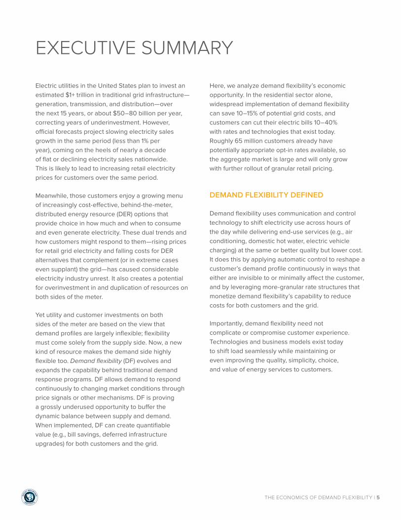
Electric utilities in the United States plan to invest an estimated $1+ trillion in traditional grid infrastructure—generation, transmission, and distribution—over the next 15 years, or about $50–80 billion per year, correcting years of underinvestment. However, official forecasts project slowing electricity sales growth in the same period (less than 1% per year), coming on the heels of nearly a decade of flat or declining electricity sales nationwide. This is likely to lead to increasing retail electricity prices for customers over the same period.

Meanwhile, those customers enjoy a growing menu of increasingly cost-effective, behind-the-meter, distributed energy resource (DER) options that provide choice in how much and when to consume and even generate electricity. These dual trends and how customers might respond to them—rising prices for retail grid electricity and falling costs for DER alternatives that complement (or in extreme cases even supplant) the grid—has caused considerable electricity industry unrest. It also creates a potential for overinvestment in and duplication of resources on both sides of the meter.

Yet utility and customer investments on both sides of the meter are based on the view that demand profiles are largely inflexible; flexibility must come solely from the supply side. Now, a new kind of resource makes the demand side highly flexible too. Demand flexibility (DF) evolves and expands the capability behind traditional demand response programs. DF allows demand to respond continuously to changing market conditions through price signals or other mechanisms. DF is proving a grossly underused opportunity to buffer the dynamic balance between supply and demand. When implemented, DF can create quantifiable value (e.g., bill savings, deferred infrastructure upgrades) for both customers and the grid.

Here, we analyze demand flexibility’s economic opportunity. In the residential sector alone, widespread implementation of demand flexibility can save 10–15% of potential grid costs, and customers can cut their electric bills 10–40% with rates and technologies that exist today. Roughly 65 million customers already have potentially appropriate opt-in rates available, so the aggregate market is large and will only grow with further rollout of granular retail pricing.

DEMAND FLEXIBILITY DEFINED

Demand flexibility uses communication and control technology to shift electricity use across hours of the day while delivering end-use services (e.g., air conditioning, domestic hot water, electric vehicle charging) at the same or better quality but lower cost. It does this by applying automatic control to reshape a customer’s demand profile continuously in ways that either are invisible to or minimally affect the customer, and by leveraging more-granular rate structures that monetize demand flexibility’s capability to reduce costs for both customers and the grid.

Importantly, demand flexibility need not complicate or compromise customer experience. Technologies and business models exist today to shift load seamlessly while maintaining or even improving the quality, simplicity, choice, and value of energy services to customers.

EXECUTIVE SUMMARY

RO

C

KY MOUNTAIN

INSTIT UTE


EXECUTIVE SUMMARY

THE EMERGING VALUE OF FLEXIWATTS: THE BROADER OPPORTUNITY FOR DERs TO LOWER GRID COSTS

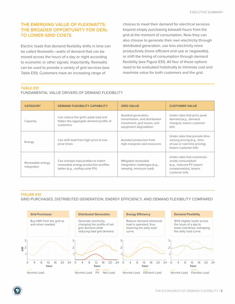
Electric loads that demand flexibility shifts in time can be called flexiwatts—watts of demand that can be moved across the hours of a day or night according to economic or other signals. Importantly, flexiwatts can be used to provide a variety of grid services (see Table ES1). Customers have an increasing range of

choices to meet their demand for electrical services beyond simply purchasing kilowatt-hours from the grid at the moment of consumption. Now they can also choose to generate their own electricity through distributed generation, use less electricity more productively (more-efficient end-use or negawatts), or shift the timing of consumption through demand flexibility (see Figure ES1). All four of these options need to be evaluated holistically to minimize cost and maximize value for both customers and the grid.

TABLE ES1FUNDAMENTAL VALUE DRIVERS OF DEMAND FLEXIBILITY

CATEGORY DEMAND FLEXIBILITY CAPABILITY GRID VALUE CUSTOMER VALUE

CapacityCan reduce the grid’s peak load and flatten the aggregate demand profile of customers

Avoided generation, transmission, and distribution investment; grid losses; and equipment degradation

Under rates that price peak demand (e.g., demand charges), lowers customer bills

Energy Can shift load from high-price to low-price times

Avoided production from high-marginal-cost resources

Under rates that provide time-varying pricing (e.g., time-of-use or real-time pricing), lowers customer bills

Renewable energy integration

Can reshape load profiles to match renewable energy production profiles better (e.g., rooftop solar PV)

Mitigated renewable integration challenges (e.g., ramping, minimum load)

Under rates that incentivize onsite consumption (e.g., reduced PV export compensation), lowers customer bills

kW

Reduce demand whenever load is operated, thus lowering the daily load curve.

0 4 8 12 16 20 24

1

2

3

Normal Load E�cient Load

hour

Energy E�ciency

Generate electricity, changing the profile of net grid demand while reducing total grid demand.

0 4 8 12 16 20 24

1

2

3

Normal Load PV Net Load

hour

Distributed Generation

Buy kWh from the grid as and when needed.

0 4 8 12 16 20 24

1

2

3

Normal Load

hour

Grid Purchases

Shift eligible loads across the hours of a day to lower-cost times, reshaping the daily load curve.

0 4 8 12 16 20 24

1

2

3

Normal Load Flexible Load

hour

Demand Flexibility

FIGURE ES1GRID PURCHASES, DISTRIBUTED GENERATION, ENERGY EFFICIENCY, AND DEMAND FLEXIBILITY COMPARED

RO

C

KY MOUNTAIN

INSTIT UTE


EXECUTIVE SUMMARY

FINDINGS

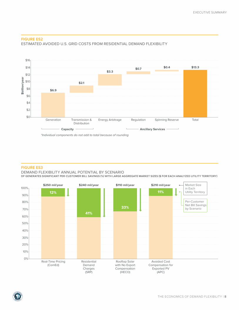
Residential demand flexibility can avoid $9 billion per year of forecast U.S. grid investment costs—more than 10% of total national forecast needs—and avoid another $4 billion per year in annual energy production and ancillary service costs.

While our analysis focuses primarily on demand flexibility’s customer-facing value, the potential grid-level cost savings from widespread demand flexibility deployment should not be ignored. Examining just two residential appliances—air conditioning and domestic water heating—shows that ~8% of U.S. peak demand could be reduced while maintaining comfort and service quality. Using industry-standard estimates of avoided costs, these peak demand savings can avoid $9 billion per year in traditional investments, including generation, transmission, and distribution. Additional costs of up to $3 billion per year can be avoided by controlling the timing of a small fraction of these appliances’ energy demands to optimize for hourly energy prices, and $1 billion per year from providing ancillary services to the grid. The total of $13 billion per year (see Figure ES2) is a conservative estimate of the economic potential of demand flexibility, because we analyze a narrow subset of flexible loads only in the residential sector, and we do not count several other benefit categories from flexibility that may add to the total value.1

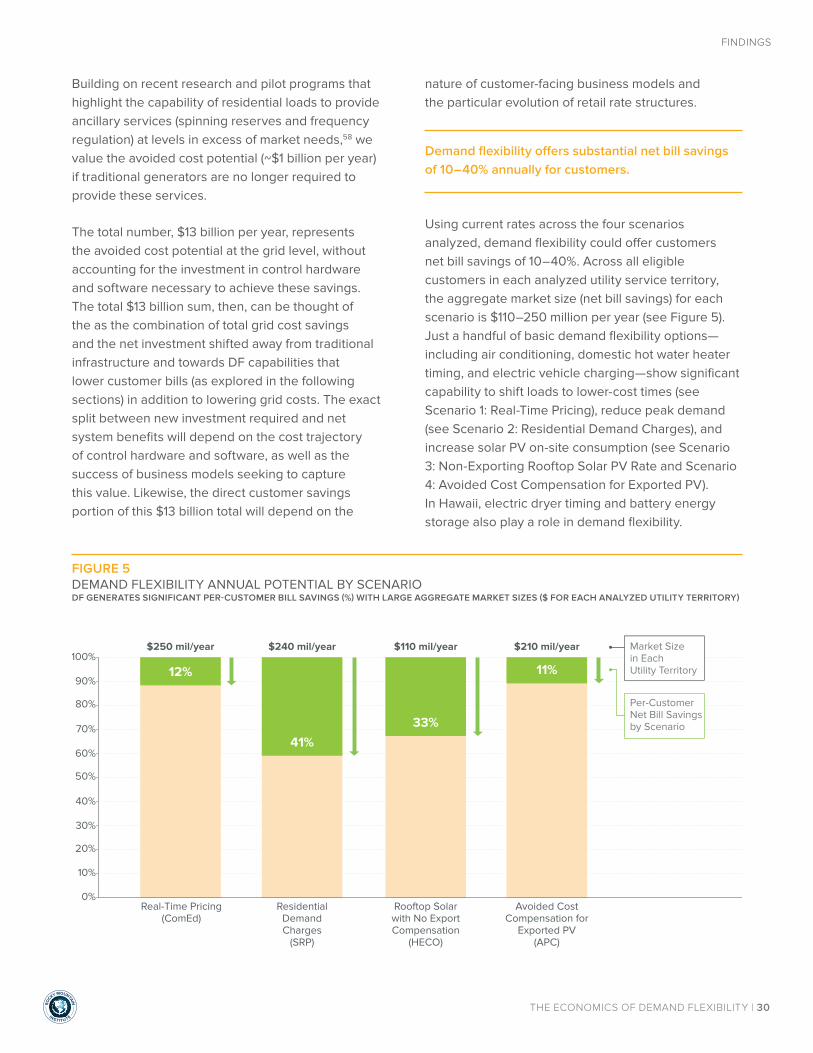
Demand flexibility offers substantial net bill savings of 10–40% annually for customers.

Using current rates across the four scenarios analyzed, demand flexibility could offer customers net bill savings of 10–40%. Across all eligible customers in each analyzed utility service territory, the aggregate market size (net bill savings) for each scenario is $110–250 million per year (see Figure ES3). Just a handful of basic demand flexibility options—including air conditioning, domestic hot water heater timing, and electric vehicle charging—show significant capability

to shift loads to lower-cost times (see Figure ES4), reduce peak demand (see Figure ES5), and increase solar PV on-site consumption (see Figure ES6). In Hawaii, electric dryer timing and battery energy storage also play a role in demand flexibility.

METHODOLOGY AND ASSUMPTIONS

We analyze the economics of demand flexibility for residential customers in two use cases across four total scenarios under specific, illustrative, real-world utility rate structures:

1. Provide bill savings by shifting energy use under granular utility rates

a. Residential real-time pricing (Commonwealth Edison, Illinois (ComEd))

b. Residential demand charges (Salt River Project, Arizona (SRP))

2. Improve the value of customer-focused distributed energy resource deployment

a. Non-export option for rooftop PV (Hawaiian Electric Company (HECO)) Proposed

b. Reduced compensation for exported PV (Alabama Power Company (APC))

We use detailed data on consumption patterns to calibrate models for demand shifting in different climates, seasons, and rate structures; and perform an economic analysis of five major demand-flexible residential loads:

• Air conditioning (AC)

• Domestic hot water (DHW)

• Electric vehicle (EV) charging

• Electric dryer cycle timing

• Battery energy storage

RO

C

KY MOUNTAIN

INSTIT UTE


EXECUTIVE SUMMARY

FIGURE ES2ESTIMATED AVOIDED U.S. GRID COSTS FROM RESIDENTIAL DEMAND FLEXIBILITY

FIGURE ES3DEMAND FLEXIBILITY ANNUAL POTENTIAL BY SCENARIODF GENERATES SIGNIFICANT PER-CUSTOMER BILL SAVINGS (%) WITH LARGE AGGREGATE MARKET SIZES ($ FOR EACH ANALYZED UTILITY TERRITORY)

$16

$10

$12

$14

$4

$6

$8

$2

$0

$6.9

$2.1

$3.3$0.7 $0.4 $13.3

$bi

llion

/yea

r

Generation

*Individual components do not add to total because of rounding

Transmission &Distribution

Energy Arbitrage Regulation Spinning Reserve Total

Capacity Ancillary Services

80%

90%

100%

50%

60%

70%

20%

30%

40%

10%

0%Real-Time Pricing

(ComEd)

$250 mil/year

12%

Residential DemandCharges

(SRP)

$240 mil/year

41%

Rooftop Solarwith No Export Compensation

(HECO)

$110 mil/year

33%

Avoided CostCompensation for

Exported PV(APC)

$210 mil/year

11%

Per-Customer Net Bill Savingsby Scenario

Market Size in Each Utility Territory

RO

C

KY MOUNTAIN

INSTIT UTE


EXECUTIVE SUMMARY

2,000

3,000

(1,000)

1,000

(2,000)

(3,000)

< $0.01 $0.01 – $0.03 $0.03 – $0.05

hourly price ($/kWh)$0.05 – $0.07 $0.07 – $0.09 > $0.09ne

t cha

nge

in g

rid

purc

hase

s (k

Wh/

yr)

DF shifts 20% of load, decreasing high-cost purchases and increasing low-cost purchases, yielding net bill reduction

10

20

15

5

01 2 3 4 5 6 7 8 9 10 11 12

Pea

k kW

Uncontrolled monthly peak demand

DF reduces peak demand by 48% on average each month

month

HECODF increases on-site PV consumption from 53% to 89%

APCDF increases on-site PV consumption from 64% to 93%

Remaining exportsSolar PV on-site consumption in base case Additional on-site consumption with demand flexibility

FIGURE ES4SHIFTING LOADS TO LOWER-COST TIMES THROUGH DEMAND FLEXIBILITY (ComEd)DF SHIFTS LOAD FROM HIGH-COST TO LOW-COST HOURS

FIGURE ES5REDUCING PEAK DEMAND THROUGH DEMAND FLEXIBILITY (SRP) DF REDUCES PEAK CUSTOMER DEMAND BY COORDINATING LOAD TIMING TO MINIMIZE PEAKS

FIGURE ES6INCREASING SOLAR PV ON-SITE CONSUMPTION THROUGH DEMAND FLEXIBILITY (HECO & APC) DF SHIFTS LOAD TO COINCIDE WITH ROOFTOP PV PRODUCTION, INCREASING ON-SITE CONSUMPTION AND REDUCING EXPORTS

RO

C

KY MOUNTAIN

INSTIT UTE


EXECUTIVE SUMMARY

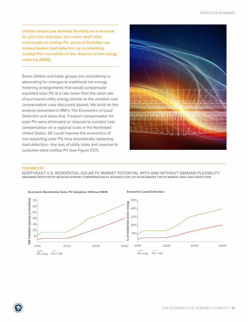
Utilities should see demand flexibility as a resource for grid cost reduction, but under retail rates unfavorable to rooftop PV, demand flexibility can instead hasten load defection by accelerating rooftop PV’s economics in the absence of net energy metering (NEM).

Some utilities and trade groups are considering or advocating for changes to traditional net energy metering arrangements that would compensate exported solar PV at a rate lower than the retail rate of purchased utility energy (similar to the avoided cost compensation case discussed above). We build on the analysis presented in RMI’s The Economics of Load Defection and show that, if export compensation for solar PV were eliminated or reduced to avoided cost compensation on a regional scale in the Northeast United States, DF could improve the economics of non-exporting solar PV, thus dramatically hastening load defection—the loss of utility sales and revenue to customer-sited rooftop PV (see Figure ES7).

20%

40%

30%

10%

50%

2015 2020 2025 2030

% o

f res

iden

tial s

ecto

r ene

rgy

Economic Load Defection

PV only PV + DF

20

40

30

10

50

70

60

2015 2020 2025 2030

GW

inst

alle

d ca

paci

ty (c

umul

ativ

e)

Economic Residential Solar PV Adoption Without NEM

PV only PV + DF

FIGURE ES7NORTHEAST U.S. RESIDENTIAL SOLAR PV MARKET POTENTIAL WITH AND WITHOUT DEMAND FLEXIBILITYASSUMING ROOFTOP PV RECEIVES EXPORT COMPENSATION AT AVOIDED COST, DF ACCELERATES THE PV MARKET AND LOAD DEFECTION

RO

C

KY MOUNTAIN

INSTIT UTE


EXECUTIVE SUMMARY

IMPLICATIONS

Demand flexibility represents a large, cost-effective, and largely untapped opportunity to reduce customer bills and grid costs. It can also give customers significant ability to protect the value proposition of rooftop PV and adapt to changing rate designs. Business models that are based on leveraging flexiwatts can be applied to as many as 65 million customers today that have access to existing opt-in granular rates, with no new regulation, technology, or policy required. Given the benefits, broad applicability, and cost-effectiveness, the widespread adoption of DF technology and business models should be a near-term priority for stakeholders across the electricity sector.

Third-party innovators: pursue opportunities now to hone customer value proposition

Many different kinds of companies can capture the value of flexiwatts, including home energy management system providers, solar PV developers, demand response companies, and appliance manufacturers, among others. These innovators can take the following actions to capitalize on the demand flexibility opportunity:

1. Take advantage of opportunities that exist today to empower customers and offer products and services to complement or compete with traditional, bundled utility energy sales.

2. Offer the customer more than bill savings; recognize that customers will want flexibility technologies for reasons other than cost alone.

3. Pursue standardized and secure technology, integrated at the factory, in order to reduce costs and scale demand flexibility faster.

4. Partner with utilities to monetize demand flexibility in front of the meter, through the provision of additional services that reduce grid costs further.

Utilities: leverage well-designed rates to reduce grid costs

Utilities of all types—vertically integrated, wires-only, retail providers, etc.—can capture demand flexibility’s grid value by taking the following steps:

1. Introduce and promote rates that reflect marginal costs, in order to ensure that customer bill reduction (and thus, utility revenue reduction) can also lead to meaningful grid cost decreases.

2. Consider flexiwatts as a resource for grid cost reduction, and not solely as a threat to revenues.

3. Harness enabling technology and third-party innovation by coupling rate offerings with technology and new customer-facing business models that promote bill savings and grid cost reduction.

Regulators: promote flexiwatts as a least-cost solution to grid challenges

State regulators have a role to play in requiring utilities to consider and fully value demand flexibility as a low-cost resource that can reduce grid-level system costs and customer bills. Regulators should consider the following:

1. Recognize the cost advantage of demand flexibility, and require utilities to consider flexiwatts as a potentially lower-cost alternative to a subset of traditional grid infrastructure investment needs.

2. Encourage utilities to offer a variety of rates to promote customer choice, balancing the potential complexity of highly granular rates against the large value proposition for customers and the grid.

3. Encourage utilities to seek partnerships that couple rate design with technology and third-party innovators to provide customers with a simple, lower cost experience.

INTRODUCTION

01

holb

ox/

Shu

tte

rsto

ck.c

om

RO

C

KY MOUNTAIN

INSTIT UTE


INTRODUCTION

THE GROWING GRID INVESTMENT CHALLENGE

The United States electric grid will need an estimated $1–1.5 trillion of investment in the next 15 years, assuming no change in how it’s planned and run. This includes $505 billion in generation resources, nearly $300 billion in transmission, and more than $580 billion in distribution assets.2 These investments will partly correct years of underinvestment.3

Historically, power-system investments have been recovered from residential and small-commercial customers in mostly volumetric, bundled charges assessed per kilowatt-hour (kWh). This was acceptable when electricity consumption grew by an average 4.6% per year from 1950 to 2010, but that demand growth has stagnated. U.S. electricity retail sales to ultimate customers peaked in 2007 and have drifted down ever since,4 falling in five of the past seven years. The U.S. Energy Information Administration’s (EIA) Annual Energy Outlook 2015 projects demand growth of 0.8% per year through 2040, with residential usage growing just 0.5%.

Moreover, while total retail sales overall are flat or falling, both peak demand and the ratio of peak to average demand have been rising across most of the country.5 This creates a significant challenge: How to pay for the grid’s needed investment when sales are stagnating? And will the grid require as much investment as forecasts suggest, or might there now exist another path based on new opportunities?

The growth of peak demand could justify infrastructure upgrades, including construction of combustion turbines that may operate expensively for just a few hours per year to meet peak demand.6 But investment required for new infrastructure and to maintain and replace aging infrastructure cannot be sustainably recovered in an era of stagnant electricity sales, especially not without raising retail prices under current volumetric

rate structures for residential customers.7 Those prices have been steadily climbing and official forecasts anticipate further increases,8 encouraging efficiency and hence further demand reduction. Without positing that these trends might create a “death spiral” of rising price and falling demand, one can still easily see the seeds of worrisome contradictions in current U.S. electricity trends.

THE RISE OF DISTRIBUTED ENERGY RESOURCES

Meanwhile, the grid—and customers’ relationship with it—are changing in big ways that offer an alternative to the massive expansion of large, centralized generation, transmission, and distribution assets. A growing range of customer-sited distributed energy resources (DERs)—including low-cost distributed generation, load control, energy storage, and end-use efficiency—offer electricity customers new choices for how and when to consume and even generate electricity. Collectively, these new resources can complement, compete with, and perhaps even displace the ~1,000 GW of existing centralized generators and their grids.

In many cases, behind-the-meter DERs can mitigate these investment needs at much lower total cost. However, utilities and regulators are inconsistent in accounting fully for the costs and benefits of DERs, so many utilities continue to emphasize traditional generation and transmission and distribution investments.9 Meanwhile, customers and third-party providers will probably continue investing in behind-the-meter energy solutions at unprecedented rates.10 This threatens a vicious cycle of over-investment and duplication of resources on both sides of the meter.

INTRODUCTION

RO

C

KY MOUNTAIN

INSTIT UTE


INTRODUCTION

REVISITING ASSUMPTIONS ABOUT ELECTRICITY SUPPLY AND DEMAND

Yet utility and customer investments on both sides of the meter are based on a fundamental assumption that now requires significant revisiting: balancing reliable generation (supply) to meet end-use demand based on inflexible demand profiles. This asymmetrical view, where flexibility must come solely from the supply side, is no longer necessary or helpful, thanks to a new kind of resource that makes the demand side highly flexible too. Demand flexibility (DF) evolves and expands the capability behind traditional demand response (DR) programs. DF allows demand to respond continuously to changing market conditions through price signals or other mechanisms. DF is proving a grossly underused opportunity to buffer the dynamic balance between supply and demand. When implemented, DF can create quantifiable value (e.g., bill savings, deferred infrastructure upgrades) for both customers and the grid.

While DF’s capability is not new, three trends make now the right time to seize its benefits: a) communications and control technologies have become cheap, powerful, and ubiquitous; b) utility rate structures are becoming sufficiently granular (e.g., real-time pricing, residential demand charges), and c) business models are emerging and maturing that can deliver DF along with other highly attractive customer value propositions (e.g., rooftop PV bundled with energy management software).

DEMAND FLEXIBILITY DEFINED

Demand flexibility uses communication and control technology to shift electricity use across hours of the day while delivering end-use services (e.g., air conditioning, domestic hot water, electric vehicle charging) at the same or better quality but lower cost.

Demand flexibility combines two core elements:

1. It applies automatic control to reshape a customer’s demand profile continuously in ways that either are invisible to the customer (e.g., decoupling the timing of grid-use from end-use through storage) or minimally affect the customer (e.g., shifting the timing of non-critical loads within customer-set thresholds).

2. For grid-connected customers, it leverages more-granular rate structures (e.g., time-of-use or real-time pricing, demand charges, distributed solar PV export pricing) to provide clear retail price signals—either directly to customers or through third-party aggregators—that monetize DF’s capability to reduce costs for both customers and the grid.

Importantly, DF need not complicate or compromise customer experience. Technologies and business models exist today to shift load seamlessly while maintaining or even improving the quality, simplicity, choice, and value of energy services to customers.

RO

C

KY MOUNTAIN

INSTIT UTE


INTRODUCTION

THE EMERGING VALUE OF FLEXIWATTS

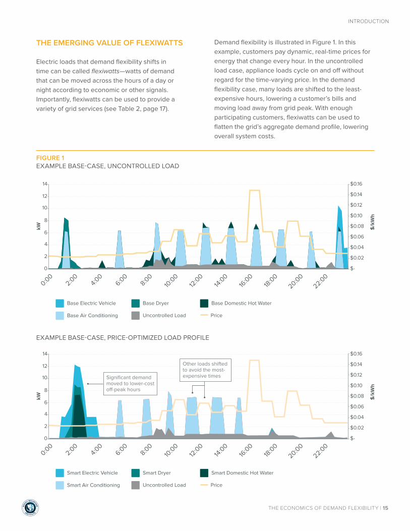
Electric loads that demand flexibility shifts in time can be called flexiwatts—watts of demand that can be moved across the hours of a day or night according to economic or other signals. Importantly, flexiwatts can be used to provide a variety of grid services (see Table 2, page 17).

Demand flexibility is illustrated in Figure 1. In this example, customers pay dynamic, real-time prices for energy that change every hour. In the uncontrolled load case, appliance loads cycle on and off without regard for the time-varying price. In the demand flexibility case, many loads are shifted to the least-expensive hours, lowering a customer’s bills and moving load away from grid peak. With enough participating customers, flexiwatts can be used to flatten the grid’s aggregate demand profile, lowering overall system costs.

Uncontrolled Load Profile

10

12

14

4

6

8

2

0

$0.14

$0.16

$0.12

$0.10

$0.08

$0.06

$0.04

$0.02

$-

kW $/k

Wh

0:00

2:00

4:00

6:00

8:00

10:0

012

:00

14:0

016

:00

18:0

020:0

022:0

0

Base Electric Vehicle Base Dryer Base Domestic Hot Water

Base Air Conditioning Uncontrolled Load Price

Price-Optimized Load Profile

10

12

14

4

6

8

2

0

$0.14

$0.16

$0.12

$0.10

$0.08

$0.06

$0.04

$0.02

$-

kW $/k

Wh

Smart Electric Vehicle Smart Dryer Smart Domestic Hot Water

Smart Air Conditioning Uncontrolled Load Price

0:00

2:00

4:00

6:00

8:00

10:0

012

:00

14:0

016

:00

18:0

020:0

022:0

0

Significant demand moved to lower-cost o�-peak hours

Other loads shifted to avoid the most-expensive times

FIGURE 1EXAMPLE BASE-CASE, UNCONTROLLED LOAD

EXAMPLE BASE-CASE, PRICE-OPTIMIZED LOAD PROFILE

RO

C

KY MOUNTAIN

INSTIT UTE


INTRODUCTION

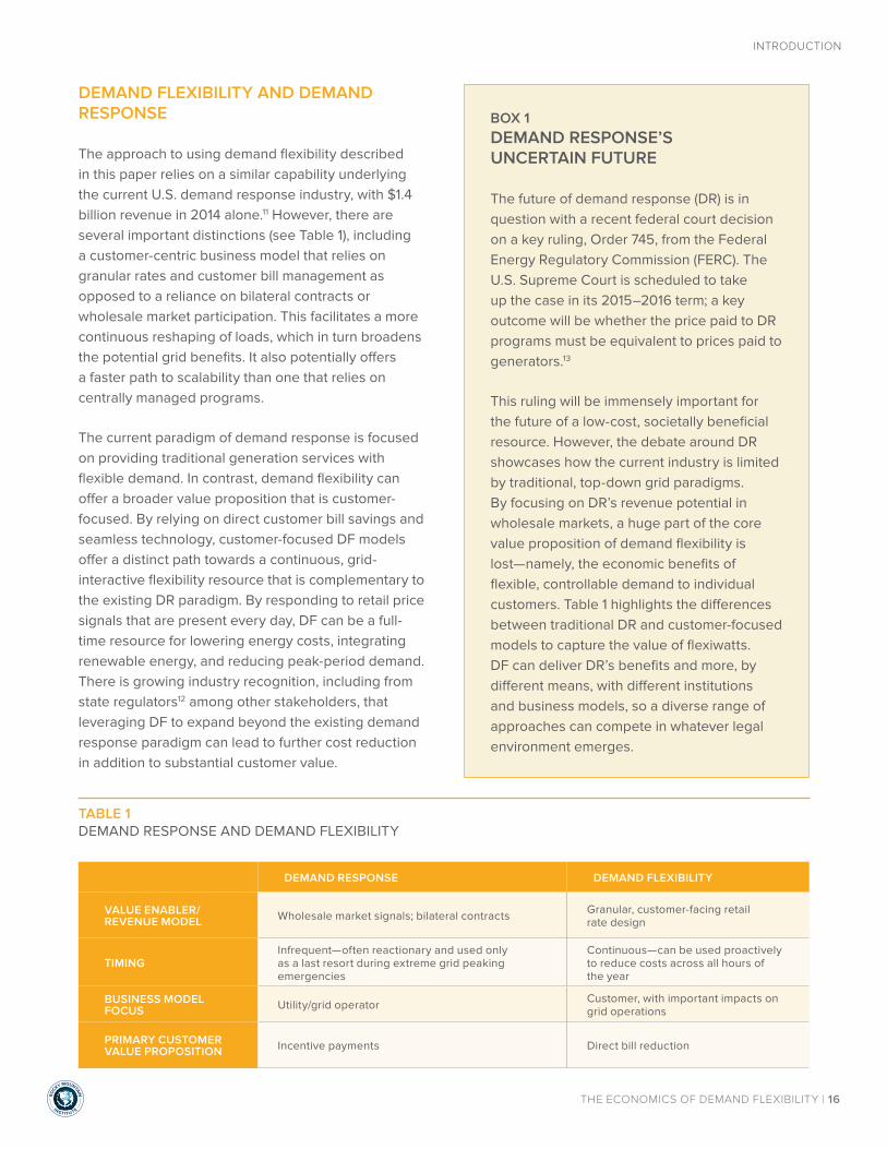
DEMAND FLEXIBILITY AND DEMAND RESPONSE

The approach to using demand flexibility described in this paper relies on a similar capability underlying the current U.S. demand response industry, with $1.4 billion revenue in 2014 alone.11 However, there are several important distinctions (see Table 1), including a customer-centric business model that relies on granular rates and customer bill management as opposed to a reliance on bilateral contracts or wholesale market participation. This facilitates a more continuous reshaping of loads, which in turn broadens the potential grid benefits. It also potentially offers a faster path to scalability than one that relies on centrally managed programs.

The current paradigm of demand response is focused on providing traditional generation services with flexible demand. In contrast, demand flexibility can offer a broader value proposition that is customer-focused. By relying on direct customer bill savings and seamless technology, customer-focused DF models offer a distinct path towards a continuous, grid-interactive flexibility resource that is complementary to the existing DR paradigm. By responding to retail price signals that are present every day, DF can be a full-time resource for lowering energy costs, integrating renewable energy, and reducing peak-period demand. There is growing industry recognition, including from state regulators12 among other stakeholders, that leveraging DF to expand beyond the existing demand response paradigm can lead to further cost reduction in addition to substantial customer value.

BOX 1DEMAND RESPONSE’S UNCERTAIN FUTURE

The future of demand response (DR) is in question with a recent federal court decision on a key ruling, Order 745, from the Federal Energy Regulatory Commission (FERC). The U.S. Supreme Court is scheduled to take up the case in its 2015–2016 term; a key outcome will be whether the price paid to DR programs must be equivalent to prices paid to generators.13

This ruling will be immensely important for the future of a low-cost, societally beneficial resource. However, the debate around DR showcases how the current industry is limited by traditional, top-down grid paradigms. By focusing on DR’s revenue potential in wholesale markets, a huge part of the core value proposition of demand flexibility is lost—namely, the economic benefits of flexible, controllable demand to individual customers. Table 1 highlights the differences between traditional DR and customer-focused models to capture the value of flexiwatts. DF can deliver DR’s benefits and more, by different means, with different institutions and business models, so a diverse range of approaches can compete in whatever legal environment emerges.

TABLE 1DEMAND RESPONSE AND DEMAND FLEXIBILITY

DEMAND RESPONSE DEMAND FLEXIBILITY

VALUE ENABLER/REVENUE MODEL Wholesale market signals; bilateral contracts Granular, customer-facing retail

rate design

TIMINGInfrequent—often reactionary and used only as a last resort during extreme grid peaking emergencies

Continuous—can be used proactively to reduce costs across all hours of the year

BUSINESS MODEL FOCUS Utility/grid operator Customer, with important impacts on

grid operations

PRIMARY CUSTOMER VALUE PROPOSITION Incentive payments Direct bill reduction

RO

C

KY MOUNTAIN

INSTIT UTE


INTRODUCTION

DEMAND FLEXIBILITY IN CONTEXT: THE BROADER OPPORTUNITY FOR DERs TO LOWER GRID COSTS

Customers have an increasing range of choices to meet their demand for electricity beyond simply purchasing it from the grid at the time of consumption. They also now have the opportunity to generate their own electricity through distributed generation, avoid the need for electricity through energy efficiency (i.e., negawatts), or shift the timing of consumption through demand flexibility (i.e., flexiwatts). All four of these options need to be evaluated holistically in order to minimize costs for customers and the grid (see Figure 2).

kW

Reduce demand whenever load is operated, thus lowering the daily load curve.

0 4 8 12 16 20 24

1

2

3

Normal Load E�cient Load

hour

Energy E�ciency

Generate electricity, changing the profile of net grid demand while reducing total grid demand.

0 4 8 12 16 20 24

1

2

3

Normal Load PV Net Load

hour

Distributed Generation

Buy kWh from the grid as and when needed.

0 4 8 12 16 20 24

1

2

3

Normal Load

hour

Grid Purchases

Shift eligible loads across the hours of a day to lower-cost times, reshaping the daily load curve.

0 4 8 12 16 20 24

1

2

3

Normal Load Flexible Load

hour

Demand Flexibility

FIGURE 2GRID PURCHASES, DISTRIBUTED GENERATION, ENERGY EFFICIENCY, AND DEMAND FLEXIBILITY COMPARED

TABLE 2FUNDAMENTAL VALUE DRIVERS OF DEMAND FLEXIBILITY

CATEGORY DEMAND FLEXIBILITY CAPABILITY GRID VALUE CUSTOMER VALUE

Capacity

Can reduce the grid’s peak load and flatten the aggregate demand profile of customers

Avoided generation, transmission, and distribution investment; grid losses; and equipment degradation

Under rates that price peak demand (e.g., demand charges), lowers customer bills

Energy Can shift load from high-price to low-price times

Avoided production from high-marginal-cost resources

Under rates that provide time-varying pricing (e.g., time-of-use or real-time pricing), lowers customer bills

Renewable energy integration

Can reshape load profiles to match renewable energy production profiles better (e.g., rooftop PV)

Mitigated renewable integration challenges (e.g., ramping, minimum load)

Under rates that incentivize on-site consumption (e.g., reduced PV export compensation), lowers customer bills

RO

C

KY MOUNTAIN

INSTIT UTE


INTRODUCTION

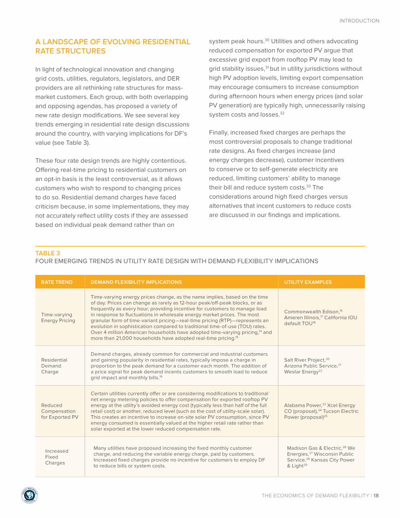
A LANDSCAPE OF EVOLVING RESIDENTIAL RATE STRUCTURES

In light of technological innovation and changing grid costs, utilities, regulators, legislators, and DER providers are all rethinking rate structures for mass-market customers. Each group, with both overlapping and opposing agendas, has proposed a variety of new rate design modifications. We see several key trends emerging in residential rate design discussions around the country, with varying implications for DF’s value (see Table 3).

These four rate design trends are highly contentious. Offering real-time pricing to residential customers on an opt-in basis is the least controversial, as it allows customers who wish to respond to changing prices to do so. Residential demand charges have faced criticism because, in some implementations, they may not accurately reflect utility costs if they are assessed based on individual peak demand rather than on

system peak hours.30 Utilities and others advocating reduced compensation for exported PV argue that excessive grid export from rooftop PV may lead to grid stability issues,31 but in utility jurisdictions without high PV adoption levels, limiting export compensation may encourage consumers to increase consumption during afternoon hours when energy prices (and solar PV generation) are typically high, unnecessarily raising system costs and losses.32

Finally, increased fixed charges are perhaps the most controversial proposals to change traditional rate designs. As fixed charges increase (and energy charges decrease), customer incentives to conserve or to self-generate electricity are reduced, limiting customers’ ability to manage their bill and reduce system costs.33 The considerations around high fixed charges versus alternatives that incent customers to reduce costs are discussed in our findings and implications.

TABLE 3FOUR EMERGING TRENDS IN UTILITY RATE DESIGN WITH DEMAND FLEXIBILITY IMPLICATIONS

RATE TREND DEMAND FLEXIBILITY IMPLICATIONS UTILITY EXAMPLES

Time-varying Energy Pricing

Time-varying energy prices change, as the name implies, based on the time of day. Prices can change as rarely as 12-hour peak/off-peak blocks, or as frequently as every hour, providing incentive for customers to manage load in response to fluctuations in wholesale energy market prices. The most granular form of time-variant pricing—real-time pricing (RTP)—represents an evolution in sophistication compared to traditional time-of-use (TOU) rates. Over 4 million American households have adopted time-varying pricing,14 and more than 21,000 households have adopted real-time pricing.15

Commonwealth Edison,16 Ameren Illinois,17 California IOU default TOU18

Residential Demand Charge

Demand charges, already common for commercial and industrial customers and gaining popularity in residential rates, typically impose a charge in proportion to the peak demand for a customer each month. The addition of a price signal for peak demand incents customers to smooth load to reduce grid impact and monthly bills.19

Salt River Project,20 Arizona Public Service,21 Westar Energy22

Reduced Compensation for Exported PV

Certain utilities currently offer or are considering modifications to traditional net energy metering policies to offer compensation for exported rooftop PV energy at the utility’s avoided energy cost (typically less than half of the full retail cost) or another, reduced level (such as the cost of utility-scale solar). This creates an incentive to increase on-site solar PV consumption, since PV energy consumed is essentially valued at the higher retail rate rather than solar exported at the lower reduced compensation rate.

Alabama Power,23 Xcel Energy CO (proposal),24 Tucson Electric Power (proposal)25

Increased Fixed Charges

Many utilities have proposed increasing the fixed monthly customer charge, and reducing the variable energy charge, paid by customers. Increased fixed charges provide no incentive for customers to employ DF to reduce bills or system costs.

Madison Gas & Electric,26 We Energies,27 Wisconsin Public Service,28 Kansas City Power & Light29

RO

C

KY MOUNTAIN

INSTIT UTE


INTRODUCTION

DEMAND FLEXIBILITY DOES NOT REQUIRE INCREASED COMPLEXITY FOR CUSTOMERS

More-granular rates that better align grid costs with customer prices can help fully capture demand flexibility’s value, but increased granularity does not necessarily require increased complexity in the customer experience. Third parties (or utilities) can offer customers services in order to simplify the experience of responding to these rates. For example, there are already successful examples of customer-facing programs that automate appliance response to grid signals without requiring customer intervention,34 and major solar companies have already announced plans to offer customers PV-integrated home energy management solutions.35

Indeed, granular rates can and should be developed in concert with technology and business model development by third-party providers; doing so would minimize the lag between a new rate and the technology to benefit from it, reduce uncertainty around revenue changes from the introduction of new rates, and ensure that a simple customer experience is available.

In the analysis that follows, we assess the underlying economics of DF from the customer perspective under more sophisticated rates, but recognize that innovative third-party business models are likely to help scale this market much faster by enabling seamless, automatic response and other values beyond cost savings, rather than relying on individual customer actions.

RO

C

KY MOUNTAIN

INSTIT UTE


INTRODUCTION

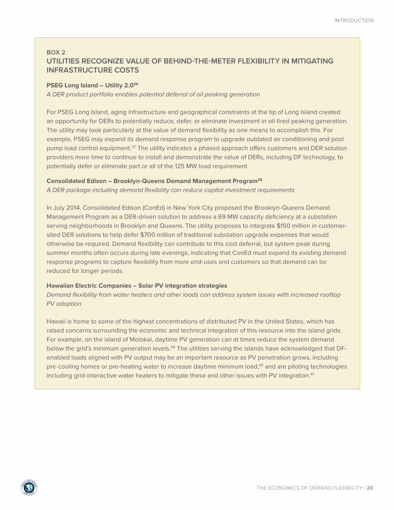
BOX 2UTILITIES RECOGNIZE VALUE OF BEHIND-THE-METER FLEXIBILITY IN MITIGATING INFRASTRUCTURE COSTS

PSEG Long Island – Utility 2.036

A DER product portfolio enables potential deferral of oil peaking generation

For PSEG Long Island, aging infrastructure and geographical constraints at the tip of Long Island created an opportunity for DERs to potentially reduce, defer, or eliminate investment in oil-fired peaking generation. The utility may look particularly at the value of demand flexibility as one means to accomplish this. For example, PSEG may expand its demand response program to upgrade outdated air conditioning and pool pump load control equipment.37 The utility indicates a phased approach offers customers and DER solution providers more time to continue to install and demonstrate the value of DERs, including DF technology, to potentially defer or eliminate part or all of the 125 MW load requirement.

Consolidated Edison – Brooklyn-Queens Demand Management Program38

A DER package including demand flexibility can reduce capital investment requirements

In July 2014, Consolidated Edison (ConEd) in New York City proposed the Brooklyn-Queens Demand Management Program as a DER-driven solution to address a 69 MW capacity deficiency at a substation serving neighborhoods in Brooklyn and Queens. The utility proposes to integrate $150 million in customer-sited DER solutions to help defer $700 million of traditional substation upgrade expenses that would otherwise be required. Demand flexibility can contribute to this cost deferral, but system peak during summer months often occurs during late evenings, indicating that ConEd must expand its existing demand response programs to capture flexibility from more end-uses and customers so that demand can be reduced for longer periods.

Hawaiian Electric Companies – Solar PV integration strategiesDemand flexibility from water heaters and other loads can address system issues with increased rooftop PV adoption

Hawaii is home to some of the highest concentrations of distributed PV in the United States, which has raised concerns surrounding the economic and technical integration of this resource into the island grids. For example, on the island of Molokai, daytime PV generation can at times reduce the system demand below the grid’s minimum generation levels.39 The utilities serving the islands have acknowledged that DF-enabled loads aligned with PV output may be an important resource as PV penetration grows, including pre-cooling homes or pre-heating water to increase daytime minimum load,40 and are piloting technologies including grid-interactive water heaters to mitigate these and other issues with PV integration.41

SCENARIOS, METHODOLOGY, AND ASSUMPTIONS

02

holb

ox/

Shu

tte

rsto

ck.c

om

RO

C

KY MOUNTAIN

INSTIT UTE



SCENARIOS FOR DEMAND FLEXIBILITY ANALYSIS

We identify four utility territories across the United States that offer different rate structures across a wide range of climates, demographics, and technology potential (see Table 4). We focus on two core use cases for demand flexibility: 1) lowering customer bills by optimizing consumption in response to time-varying energy and demand pricing, and 2) increasing on-site consumption of rooftop PV in the absence of net energy metering (NEM).

The analyzed examples show DF’s potential in the context of real or prospective market scenarios only. They are not an endorsement of the specific rate structures and/or utilities we examine. There is room for debate about the relative merits and specific design considerations of real-time pricing, demand charges, and on-site consumption incentives. We use these scenarios to demonstrate the economic value of DF today and demonstrate examples of the broad economic potential to deploy flexiwatts as rate structures evolve.


TABLE 4RATE STRUCTURES EXAMINED IN THIS REPORT

USE CASE RATE STRUCTURE ANALYZED

Lowering customer bills by optimizing consumption in response to time-varying energy and demand pricing

1. Residential real-time pricing

Utility Example: Commonwealth Edison (ComEd) – Illinois42

Status: Option for all customers

ComEd offers a real-time pricing option to residential customers, where the hourly energy price charged to customers is derived from nodal prices paid by ComEd to the regional transmission operator, PJM. We analyze the potential cost savings of each controlled load, optimizing its demand profile in response to real-time prices.

2. Demand charges for solar PV customers

Utility Example: Salt River Project (SRP) – Arizona43

Status: Mandatory for new PV customers

SRP recently approved a rate plan for new PV customers that includes an additional fixed charge as well as a monthly peak demand charge. We analyze the value of each load in reducing the peak demand on the utility side of the customer meter.

Increasing on-site consumption of rooftop solar PV in the absence of net energy metering

3. No compensation for exported PV proposal

Utility Example: Hawaiian Electric Co. (HECO) – Hawaii44

Status: Proposed option for new PV customers

In an April 2014 order, the Hawaii Public Service Commission directed HECO to propose changes to its interconnection procedures that would favor customers with non-exporting PV systems. We analyze the capability of DF to increase on-site consumption of rooftop PV generation when the value of exported generation is zero.

4. Avoided cost compensation for exported PV

Utility Example: Alabama Power (APC) – Alabama45

Status: Mandatory for all PV customers

Alabama Power offers solar PV customers export compensation at the utility’s avoided energy cost, which is less than half the retail rate. As with the HECO scenario, we analyze the capability of DF to increase on-site consumption of rooftop PV generation.

RO

C

KY MOUNTAIN

INSTIT UTE



METHODOLOGY AND ASSUMPTIONS

To develop baseline customer electricity usage models, we use 15-minute submetered home energy data from the Northwest Energy Efficiency Alliance (NEEA), collected between 2012 and 2013, to derive typical profiles for behavior-driven appliance use (e.g., hot water and electric dryers), as well as estimates for non-flexible load in a typical home (e.g., television, cooking, lights, etc.). We discuss in the following sections how we account for location-specific, weather-driven loads like heating and air conditioning in each scenario (see Appendix B for a more detailed explanation of this methodology).

To estimate rooftop solar PV production in the three scenarios in which solar is modeled, we use weather data with the National Renewable Energy Laboratory’s (NREL) PVWatts hourly production modeling tool, and interpolate to a 15-minute resolution. We use NREL’s System Advisor Model (SAM) with the state-specific assumptions listed in Appendix B to calculate levelized cost of third-party-owned rooftop PV in each applicable scenario geography.

Load modeling methodology

For this analysis, we model the potential for four major electricity loads to be shifted in time: air conditioning, electric water heaters, electric dryers, and electric vehicle charging. We also model dedicated battery storage as a point of comparison. We analyze the savings potential of shifting from high-cost times to low-cost times (or from outside a PV generation period to inside a PV generation period) based on the specific cost drivers for customers in each modeled scenario: hourly price, peak demand, and PV output. Appendix C has a detailed description of the appliance- and rate structure-specific models used to minimize costs.

We model demand flexibility for each appliance over a full year in 15-minute increments in order to capture the impacts of changing weather, energy consumption, and solar PV production on the value of demand flexibility, as well as to capture the billing interval duration over which peak demand charges are assessed (30-minute for SRP, 60-minute for ComEd).

RO

C

KY MOUNTAIN

INSTIT UTE



Each flexible load has different customized constraints and operating requirements:

• Domestic electric hot water (DHW):i We shift energy consumption by heating water in the storage tank preferentially during low-cost periods and ensuring that both a) enough hot water is present in the tank during high-cost periods so that the heating elements do not have to run, and b) there is always enough hot water in the tank to provide hot water under the same schedule to the customer as in the base uncontrolled case, for every daily profile of hot water use.

• Air conditioning (AC): We use a thermal model of a typical single-family home to derive a baseline AC consumption profile for each modeled geographic location. Modeled thermal loads include ambient air temperature-driven envelope heating as well as solar heating gains through windows, calculated using weather data and building energy modeling tools. To simulate smart controls, we impose a thermostat control strategy that pre-cools the building during low-cost periods and allows the building setpoint to rise up to 4°F during high-cost periods.ii

• Electric vehicle (EV) charging: We assume base-case drivers recharge EV batteries using a Level 1, 3-kW charger immediately upon returning from a 30-mile trip each day, with trip timing changing on weekdays (8:00 a.m. to 6:00 p.m.) versus weekends (8:00 p.m. to 11:00 p.m.). In other words, the car is unavailable for charging during the day on weekdays or on weekend evenings. In the controlled case, we optimize EV charging to occur at the least-cost hours when the vehicle is parked and plugged in, always charging to 100% by the time the driver next needs the car.

• Electric dryers: We use baseline dryer consumption profiles from the NEEA database. To optimize dryer load, we allow the start time of each cycle to shift by up to six hours in either direction to minimize total cycle costs. This can be accomplished either via behavioral change or via smart controls that allow a customer to load the dryer and delay cycle start time automatically.

As a point of comparison to demand flexibility, we model the capability of a dedicated 7 kWh/2 kW battery storage system in each of our use cases. We simulate the battery charging during low-cost hours and discharging during high-cost hours, subject to its inverter capacity and losses and its storage capacity.

i We restrict our analysis to homes with electric water heaters. EIA data indicate there are approximately 47 million residential electric water heaters in the U.S. as of 2009, representing 41% of the market.

ii Though we model this setpoint increase during all high-cost hours, our algorithm minimizes the actual temperature rise that takes place, and the savings presented here can be achieved with a very low number of high-temperature events (see Appendix C for a fuller description).

RO

C

KY MOUNTAIN

INSTIT UTE



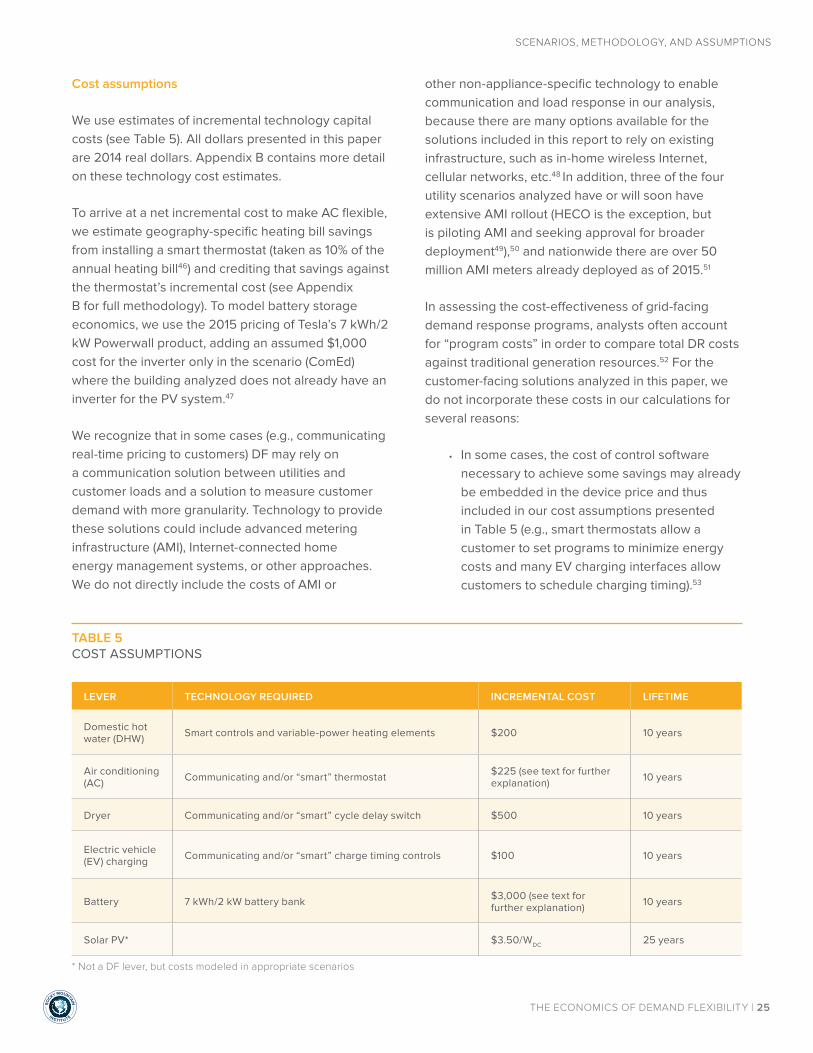
Cost assumptions

We use estimates of incremental technology capital costs (see Table 5). All dollars presented in this paper are 2014 real dollars. Appendix B contains more detail on these technology cost estimates.

To arrive at a net incremental cost to make AC flexible, we estimate geography-specific heating bill savings from installing a smart thermostat (taken as 10% of the annual heating bill46) and crediting that savings against the thermostat’s incremental cost (see Appendix B for full methodology). To model battery storage economics, we use the 2015 pricing of Tesla’s 7 kWh/2 kW Powerwall product, adding an assumed $1,000 cost for the inverter only in the scenario (ComEd) where the building analyzed does not already have an inverter for the PV system.47

We recognize that in some cases (e.g., communicating real-time pricing to customers) DF may rely on a communication solution between utilities and customer loads and a solution to measure customer demand with more granularity. Technology to provide these solutions could include advanced metering infrastructure (AMI), Internet-connected home energy management systems, or other approaches. We do not directly include the costs of AMI or

other non-appliance-specific technology to enable communication and load response in our analysis, because there are many options available for the solutions included in this report to rely on existing infrastructure, such as in-home wireless Internet, cellular networks, etc.48 In addition, three of the four utility scenarios analyzed have or will soon have extensive AMI rollout (HECO is the exception, but is piloting AMI and seeking approval for broader deployment49),50 and nationwide there are over 50 million AMI meters already deployed as of 2015.51

In assessing the cost-effectiveness of grid-facing demand response programs, analysts often account for “program costs” in order to compare total DR costs against traditional generation resources.52 For the customer-facing solutions analyzed in this paper, we do not incorporate these costs in our calculations for several reasons:

• In some cases, the cost of control software necessary to achieve some savings may already be embedded in the device price and thus included in our cost assumptions presented in Table 5 (e.g., smart thermostats allow a customer to set programs to minimize energy costs and many EV charging interfaces allow customers to schedule charging timing).53

TABLE 5COST ASSUMPTIONS

LEVER TECHNOLOGY REQUIRED INCREMENTAL COST LIFETIME

Domestic hot water (DHW) Smart controls and variable-power heating elements $200 10 years

Air conditioning (AC) Communicating and/or “smart” thermostat $225 (see text for further

explanation) 10 years

Dryer Communicating and/or “smart” cycle delay switch $500 10 years

Electric vehicle (EV) charging Communicating and/or “smart” charge timing controls $100 10 years

Battery 7 kWh/2 kW battery bank $3,000 (see text for further explanation) 10 years

Solar PV* $3.50/WDC 25 years

* Not a DF lever, but costs modeled in appropriate scenarios

RO

C

KY MOUNTAIN

INSTIT UTE



• To the extent that the bundled software does not already support the specific approaches we model in this analysis, we recognize that the approaches we use for more-dynamic control are relatively simplistic (see Appendix C), and implementing them with existing device software is likely a trivial programming change that would not add significant cost.

• We also note that solutions that depend on customer-driven and/or automated response to price signals may not have the utility overhead costs typical of centrally-managed programs, such as traditional emergency demand response programs.

We recognize that investments in energy efficiency, alone or combined with DF technologies, are likely to be a part of the minimum-cost technology bundle for customers under any of the rate structures analyzed, and that efficiency has a commensurately great potential for grid cost reductions.54 However, we focus our analysis on DF alone, in order to highlight its unique capabilities and economic value.

Market sizing assumptions

We extend the core modeling results for a single customer in each utility jurisdiction by scaling those results to estimate the savings potential, vendor market size, and PV market enabled for all eligible customers that could sign up for the rates we analyze. To scale our bill savings results to other customers served by the same utility, we first scale the consumption of our modeled customer to average residential consumption for each utility, using EIA Form 861 data from 2013. Similarly, for the capital costs of flexibility-enabling technology (i.e., controls and hardware), we scale the costs of cost-effective technology for our modeled customer to average consumption for residential customers.

For scenarios 2–4, where demand flexibility supports the value proposition of customers under PV-specific rates, we estimate the size of the PV market that DF could unlock. We estimate the number of single-family, owner-occupied homes that can support a PV system, and calculate the size of the PV installation market for these customers. Full methodology is outlined in Appendix D.

For scenarios 1 and 2, we estimate the utility-wide peak demand reduction potential unlocked by residential DF by scaling our peak demand savings estimate to average residential customer peak loads and the number of eligible customers (single-family, owner-occupied homes) by utility.55

The market size estimates we present are likely higher than the practical opportunity because many customers will not choose to adopt DF technologies even with strong economics. However, if even a fraction of the potential market adopts demand flexibility, it would still represent a large market opportunity for vendors to offer products and services that deliver bill savings to customers while lowering grid costs and improving grid operation.

In addition, the more customers that adopt DF, the more likely utilities are to react by refining offered rate structures to ensure that customer prices still reflect utility costs. For example, as more customers shift loads in response to real-time prices, it is likely to have an aggregate effect of smoothing the system load profile, and thus shrink the difference between peak and off-peak prices. Or, as more customers adopt technology to minimize peak demand, utilities may adjust demand charge magnitudes in order to true up cost recovery with expenses. The savings and market sizing results we present are thus reflective of current reality, but may change as utilities adjust rates.

RO

C

KY MOUNTAIN

INSTIT UTE



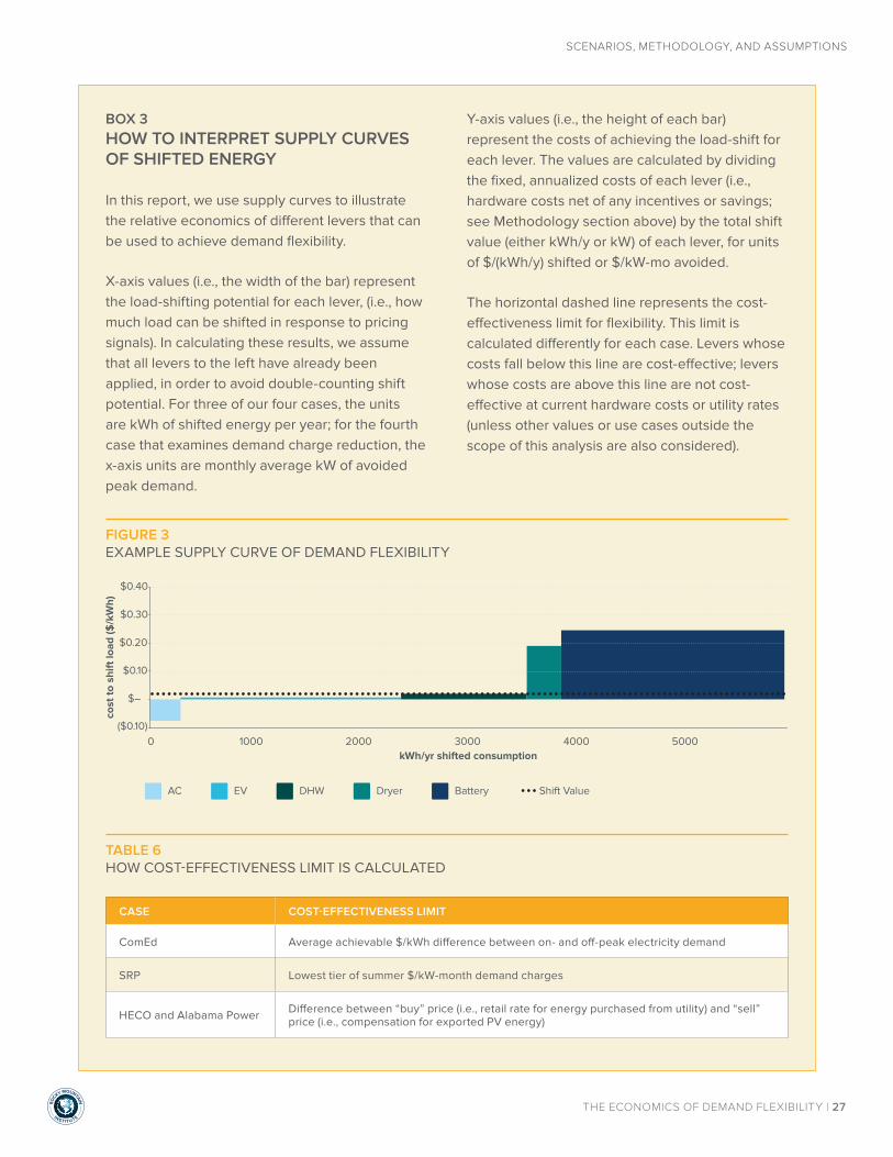
BOX 3HOW TO INTERPRET SUPPLY CURVES OF SHIFTED ENERGY

In this report, we use supply curves to illustrate the relative economics of different levers that can be used to achieve demand flexibility.

X-axis values (i.e., the width of the bar) represent the load-shifting potential for each lever, (i.e., how much load can be shifted in response to pricing signals). In calculating these results, we assume that all levers to the left have already been applied, in order to avoid double-counting shift potential. For three of our four cases, the units are kWh of shifted energy per year; for the fourth case that examines demand charge reduction, the x-axis units are monthly average kW of avoided peak demand.

Y-axis values (i.e., the height of each bar) represent the costs of achieving the load-shift for each lever. The values are calculated by dividing the fixed, annualized costs of each lever (i.e., hardware costs net of any incentives or savings; see Methodology section above) by the total shift value (either kWh/y or kW) of each lever, for units of $/(kWh/y) shifted or $/kW-mo avoided.

The horizontal dashed line represents the cost-effectiveness limit for flexibility. This limit is calculated differently for each case. Levers whose costs fall below this line are cost-effective; levers whose costs are above this line are not cost-effective at current hardware costs or utility rates (unless other values or use cases outside the scope of this analysis are also considered).

TABLE 6HOW COST-EFFECTIVENESS LIMIT IS CALCULATED

CASE COST-EFFECTIVENESS LIMIT

ComEd Average achievable $/kWh difference between on- and off-peak electricity demand

SRP Lowest tier of summer $/kW-month demand charges

HECO and Alabama Power Difference between “buy” price (i.e., retail rate for energy purchased from utility) and “sell” price (i.e., compensation for exported PV energy)

FIGURE 3EXAMPLE SUPPLY CURVE OF DEMAND FLEXIBILITY

$0.30

$0.40

$0.10

$0.20

$–

($0.10)0 1000 2000 3000 4000 5000

cost

to s

hift

load

($/k

Wh)

kWh/yr shifted consumption

AC DryerDHW Battery Shift Value

Supply Curve of Shifted Energy: ComEd

EV

FINDINGS

03

RO

C

KY MOUNTAIN

INSTIT UTE


FINDINGS

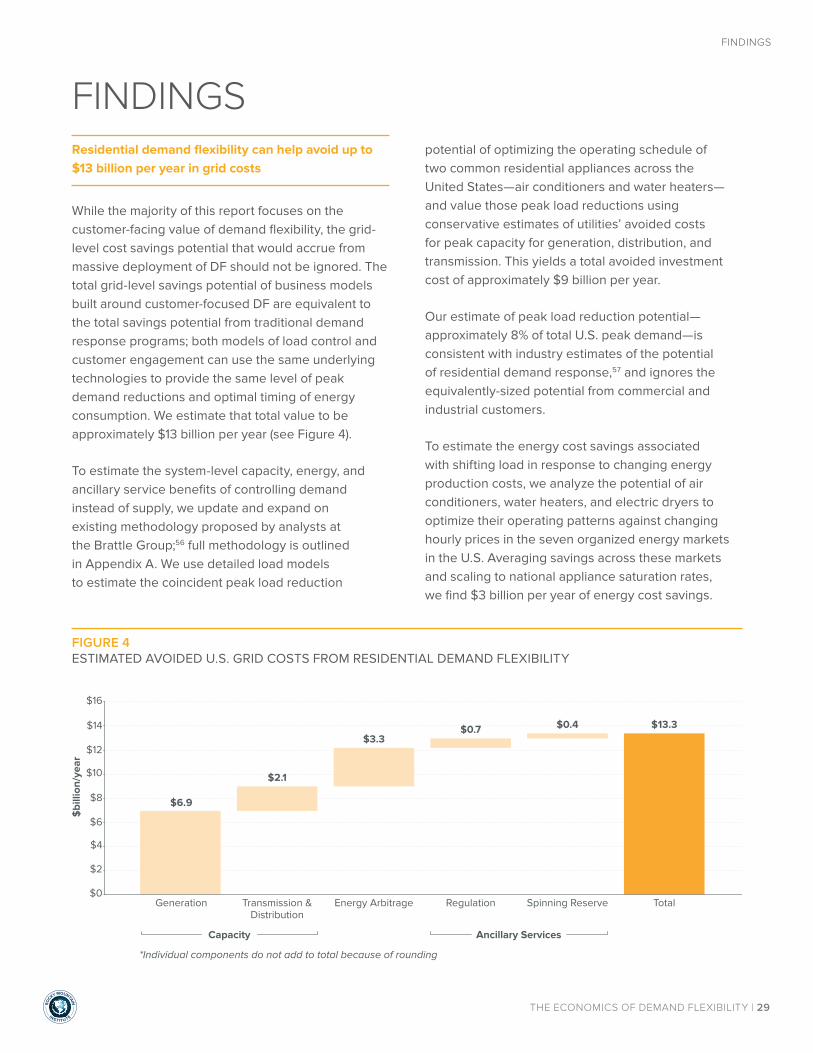
Residential demand flexibility can help avoid up to $13 billion per year in grid costs

While the majority of this report focuses on the customer-facing value of demand flexibility, the grid-level cost savings potential that would accrue from massive deployment of DF should not be ignored. The total grid-level savings potential of business models built around customer-focused DF are equivalent to the total savings potential from traditional demand response programs; both models of load control and customer engagement can use the same underlying technologies to provide the same level of peak demand reductions and optimal timing of energy consumption. We estimate that total value to be approximately $13 billion per year (see Figure 4).

To estimate the system-level capacity, energy, and ancillary service benefits of controlling demand instead of supply, we update and expand on existing methodology proposed by analysts at the Brattle Group;56 full methodology is outlined in Appendix A. We use detailed load models to estimate the coincident peak load reduction

potential of optimizing the operating schedule of two common residential appliances across the United States—air conditioners and water heaters—and value those peak load reductions using conservative estimates of utilities’ avoided costs for peak capacity for generation, distribution, and transmission. This yields a total avoided investment cost of approximately $9 billion per year.

Our estimate of peak load reduction potential—approximately 8% of total U.S. peak demand—is consistent with industry estimates of the potential of residential demand response,57 and ignores the equivalently-sized potential from commercial and industrial customers.

To estimate the energy cost savings associated with shifting load in response to changing energy production costs, we analyze the potential of air conditioners, water heaters, and electric dryers to optimize their operating patterns against changing hourly prices in the seven organized energy markets in the U.S. Averaging savings across these markets and scaling to national appliance saturation rates, we find $3 billion per year of energy cost savings.

FIGURE 4ESTIMATED AVOIDED U.S. GRID COSTS FROM RESIDENTIAL DEMAND FLEXIBILITY

$16

$10

$12

$14

$4

$6

$8

$2

$0

$6.9

$2.1

$3.3$0.7 $0.4 $13.3

$bi

llion

/yea

r

Generation

*Individual components do not add to total because of rounding

Transmission &Distribution

Energy Arbitrage Regulation Spinning Reserve Total

Capacity Ancillary Services

FINDINGS

RO

C

KY MOUNTAIN

INSTIT UTE


FINDINGS

Building on recent research and pilot programs that highlight the capability of residential loads to provide ancillary services (spinning reserves and frequency regulation) at levels in excess of market needs,58 we value the avoided cost potential (~$1 billion per year) if traditional generators are no longer required to provide these services.

The total number, $13 billion per year, represents the avoided cost potential at the grid level, without accounting for the investment in control hardware and software necessary to achieve these savings. The total $13 billion sum, then, can be thought of the as the combination of total grid cost savings and the net investment shifted away from traditional infrastructure and towards DF capabilities that lower customer bills (as explored in the following sections) in addition to lowering grid costs. The exact split between new investment required and net system benefits will depend on the cost trajectory of control hardware and software, as well as the success of business models seeking to capture this value. Likewise, the direct customer savings portion of this $13 billion total will depend on the

nature of customer-facing business models and the particular evolution of retail rate structures.

Demand flexibility offers substantial net bill savings of 10–40% annually for customers.

Using current rates across the four scenarios analyzed, demand flexibility could offer customers net bill savings of 10–40%. Across all eligible customers in each analyzed utility service territory, the aggregate market size (net bill savings) for each scenario is $110–250 million per year (see Figure 5). Just a handful of basic demand flexibility options—including air conditioning, domestic hot water heater timing, and electric vehicle charging—show significant capability to shift loads to lower-cost times (see Scenario 1: Real-Time Pricing), reduce peak demand (see Scenario 2: Residential Demand Charges), and increase solar PV on-site consumption (see Scenario 3: Non-Exporting Rooftop Solar PV Rate and Scenario 4: Avoided Cost Compensation for Exported PV). In Hawaii, electric dryer timing and battery energy storage also play a role in demand flexibility.

FIGURE 5DEMAND FLEXIBILITY ANNUAL POTENTIAL BY SCENARIODF GENERATES SIGNIFICANT PER-CUSTOMER BILL SAVINGS (%) WITH LARGE AGGREGATE MARKET SIZES ($ FOR EACH ANALYZED UTILITY TERRITORY)

80%

90%

100%

50%

60%

70%

20%

30%

40%

10%

0%Real-Time Pricing

(ComEd)

$250 mil/year

12%

Residential DemandCharges

(SRP)

$240 mil/year

41%

Rooftop Solarwith No Export Compensation

(HECO)

$110 mil/year

33%

Avoided CostCompensation for

Exported PV(APC)

$210 mil/year

11%

Per-Customer Net Bill Savingsby Scenario

Market Size in Each Utility Territory

RO

C

KY MOUNTAIN

INSTIT UTE


FINDINGS

SCENARIO 1: REAL-TIME PRICING

Finding: Demand flexibility offers 19% savings on hourly energy charges, resulting in 12% net cost savings on overall bill

In 2007, Commonwealth Edison introduced a residential real-time pricing (RTP) program. Participating customers are given day-ahead estimates of hourly energy prices, and can adapt the timing of their consumption accordingly. The energy price actually paid by customers changes every hour to reflect the market-clearing price in the wholesale energy market. We analyze the cost savings that demand flexibility offers for both a customer already on this rate structure as well as a customer on the standard, volumetric rate who could choose to opt in to the real-time pricing rate.

TABLE 7SCENARIO-SPECIFIC MODELING SETUP: RESIDENTIAL REAL-TIME PRICING

VARIABLE SCENARIO DETAIL

Utility Commonwealth Edison (ComEd)

Program name/Rate design Residential Real-Time Pricing59 (opt-in program available to all customers)

Geography (TMY3 location) Chicago, IL (O’Hare Airport)

Customers participating Approximately 10,000

Fixed charges $11.35/month

Demand charges $4.05/kW-month (based on previous year’s summer coincident peak)

Energy charges Varies hourly; 2014 average $0.042/kWh. Additional distribution, etc. costs of $0.055/kWh also collected volumetrically.

Customer PV array size analyzed None (no impact on results)

RO

C

KY MOUNTAIN

INSTIT UTE


FINDINGS

DETAILED FINDINGS

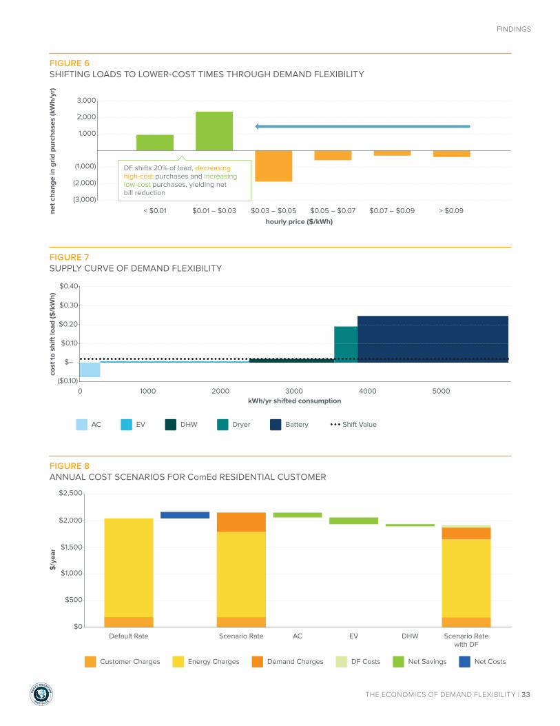
Load shifting potential

Cost-effective DF strategies can move about 20% of annual load from high-price hours to lower-price hours, with minimal impacts on comfort or convenience. A customer with an uncontrolled load profile would buy energy at an average of $0.044/kWh; with demand flexibility, that price declines nearly 19%, to $0.036/kWh.

Cost-effective flexibility bundle

In this scenario, three of the five technologies analyzed make up the most economic product bundle for customers. Smart thermostats to control air conditioning are the least-cost flexibility option: their cost of shifted energy is negative, due to the substantially lower heating cost (approximately $50/year in avoided gas costs) gained from installing a

smart thermostat. EV charging is the next most cost-effective flexibility option at $0.01 per kWh of shifted load, as well as the overall largest shift opportunity, due to the low cost of enabling controls in EV charging equipment and the large flexibility potential of vehicle battery capacity. Domestic hot water is the third most cost-effective flexibility option, shifting more than half its energy demand into lower-cost hours. DF-capable dryers and on-site electric storage batteries, at current prices, do not appear cost-effective for real-time price arbitrage under this specific rate.

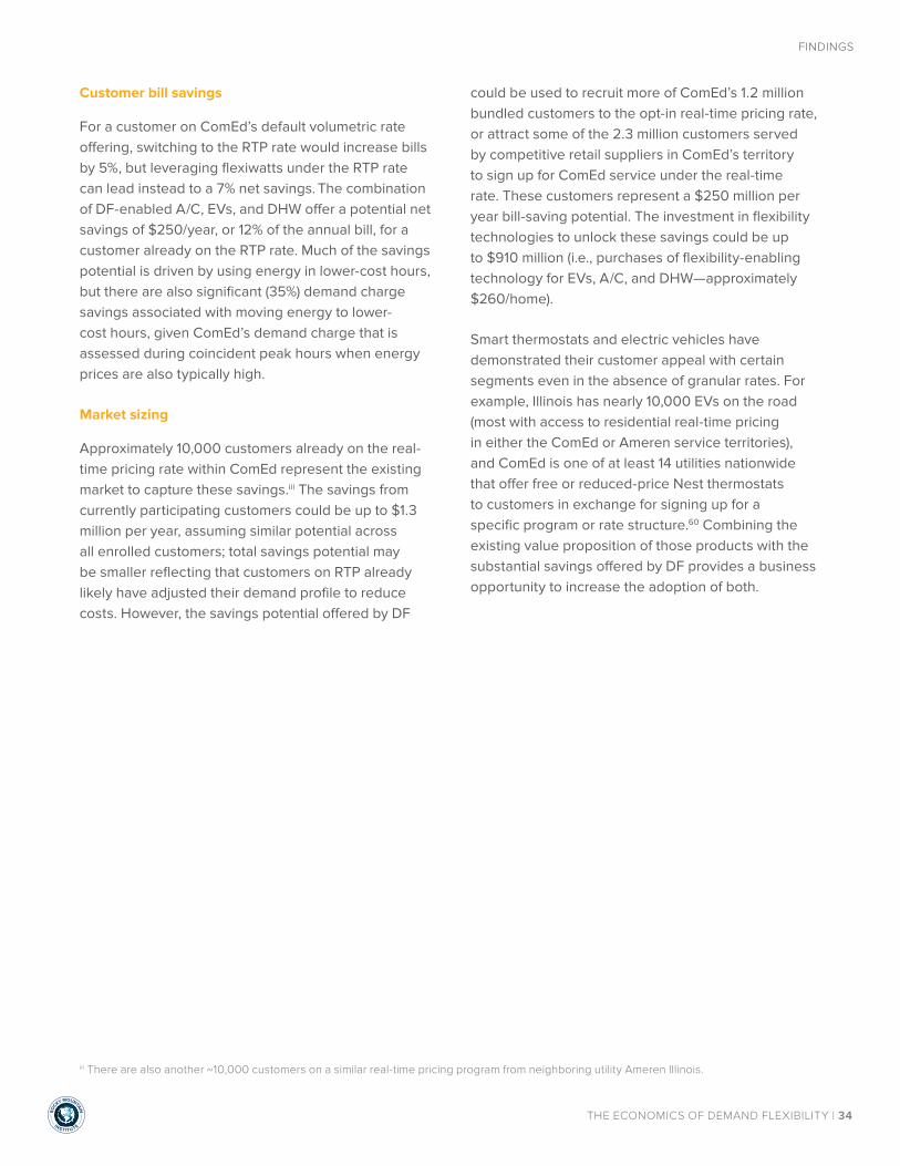
SCENARIO FINDINGS SUMMARY (ComEd)

• Cost-effective demand flexibility can shift nearly 20% of total annual kWh to lower-cost hours.

• Participating customers can save $250/year, or 12% of total bills, net of the cost of enabling technology.

• Across all 10,000 existing, participating customers, this represents a $1.3 million per year savings opportunity.

• There is a $2.6 million investment opportunity for innovative businesses to provide customers the products and services to unlock these savings (i.e., purchases of flexibility-enabling technology for EVs, A/C, and DHW—approximately $260/home).

• Customers on the default volumetric ComEd rate would save up to $140/year, or 7% of total bills, net of technology costs, if they switched to the real-time pricing rate and leveraged demand flexibility.

• Across ComEd’s 1.2 million customers, and the additional 2.3 million customers served by retail providers in ComEd’s territory, this cost-effective switch represents a net bill savings potential of up to $250 million per year.

• There is an investment opportunity of up to $910 million for vendors to help customers unlock these savings.

• If all eligible customers in ComEd territory pursued demand flexibility, the utility’s peak demand could be reduced by up to 940 MW.

RO

C

KY MOUNTAIN

INSTIT UTE


FINDINGS

FIGURE 7SUPPLY CURVE OF DEMAND FLEXIBILITY

FIGURE 8ANNUAL COST SCENARIOS FOR ComEd RESIDENTIAL CUSTOMER

FIGURE 6SHIFTING LOADS TO LOWER-COST TIMES THROUGH DEMAND FLEXIBILITY

2,000

3,000

(1,000)

1,000

(2,000)

(3,000)

< $0.01 $0.01 – $0.03 $0.03 – $0.05

hourly price ($/kWh)$0.05 – $0.07 $0.07 – $0.09 > $0.09ne

t cha

nge

in g

rid

purc

hase

s (k

Wh/

yr)

DF shifts 20% of load, decreasing high-cost purchases and increasing low-cost purchases, yielding net bill reduction

$0.30

$0.40

$0.10

$0.20

$–

($0.10)0 1000 2000 3000 4000 5000

cost

to s

hift

load

($/k

Wh)

kWh/yr shifted consumption

AC DryerDHW Battery Shift Value

Supply Curve of Shifted Energy: ComEd

EV

$2,500

$2,000

$1,500

$1,000

$500

$0

$/y

ear

Default Rate Scenario Rate AC EV DHW Scenario Ratewith DF

Customer Charges Energy Charges Demand Charges Net CostsDF Costs Net Savings

Annual Supply Costs

RO

C

KY MOUNTAIN

INSTIT UTE


FINDINGS

Customer bill savings

For a customer on ComEd’s default volumetric rate offering, switching to the RTP rate would increase bills by 5%, but leveraging flexiwatts under the RTP rate can lead instead to a 7% net savings. The combination of DF-enabled A/C, EVs, and DHW offer a potential net savings of $250/year, or 12% of the annual bill, for a customer already on the RTP rate. Much of the savings potential is driven by using energy in lower-cost hours, but there are also significant (35%) demand charge savings associated with moving energy to lower-cost hours, given ComEd’s demand charge that is assessed during coincident peak hours when energy prices are also typically high.

Market sizing

Approximately 10,000 customers already on the real-time pricing rate within ComEd represent the existing market to capture these savings.iii The savings from currently participating customers could be up to $1.3 million per year, assuming similar potential across all enrolled customers; total savings potential may be smaller reflecting that customers on RTP already likely have adjusted their demand profile to reduce costs. However, the savings potential offered by DF

could be used to recruit more of ComEd’s 1.2 million bundled customers to the opt-in real-time pricing rate, or attract some of the 2.3 million customers served by competitive retail suppliers in ComEd’s territory to sign up for ComEd service under the real-time rate. These customers represent a $250 million per year bill-saving potential. The investment in flexibility technologies to unlock these savings could be up to $910 million (i.e., purchases of flexibility-enabling technology for EVs, A/C, and DHW—approximately $260/home).

Smart thermostats and electric vehicles have demonstrated their customer appeal with certain segments even in the absence of granular rates. For example, Illinois has nearly 10,000 EVs on the road (most with access to residential real-time pricing in either the ComEd or Ameren service territories), and ComEd is one of at least 14 utilities nationwide that offer free or reduced-price Nest thermostats to customers in exchange for signing up for a specific program or rate structure.60 Combining the existing value proposition of those products with the substantial savings offered by DF provides a business opportunity to increase the adoption of both.

iii There are also another ~10,000 customers on a similar real-time pricing program from neighboring utility Ameren Illinois.

RO

C

KY MOUNTAIN

INSTIT UTE


FINDINGS

SCENARIO 2: RESIDENTIAL DEMAND CHARGES

Finding: Demand flexibility can reduce monthly peak demand by 48%, lowering net bills by over 40%

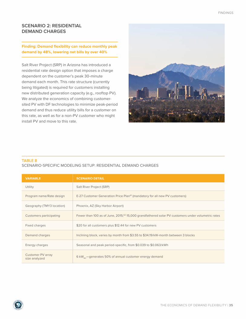
Salt River Project (SRP) in Arizona has introduced a residential rate design option that imposes a charge dependent on the customer’s peak 30-minute demand each month. This rate structure (currently being litigated) is required for customers installing new distributed generation capacity (e.g., rooftop PV). We analyze the economics of combining customer-sited PV with DF technologies to minimize peak-period demand and thus reduce utility bills for a customer on this rate, as well as for a non-PV customer who might install PV and move to this rate.

TABLE 8SCENARIO-SPECIFIC MODELING SETUP: RESIDENTIAL DEMAND CHARGES


Utility Salt River Project (SRP)

Program name/Rate design E-27 Customer Generation Price Plan61 (mandatory for all new PV customers)

Geography (TMY3 location) Phoenix, AZ (Sky Harbor Airport)

Customers participating Fewer than 100 as of June, 2015;62 15,000 grandfathered solar PV customers under volumetric rates

Fixed charges $20 for all customers plus $12.44 for new PV customers

Demand charges Inclining block, varies by month from $3.55 to $34.19/kW-month between 3 blocks

Energy charges Seasonal and peak period-specific, from $0.039 to $0.063/kWh

Customer PV array size analyzed 6 kWAC—generates 50% of annual customer energy demand

RO

C

KY MOUNTAIN

INSTIT UTE


FINDINGS

DETAILED FINDINGS

Peak demand reduction potential

By coordinating the operation of major loads to avoid high peak demand during the 1–8 pm demand charge window, the combined control strategies are able to cost-effectively reduce peak demand by 48% on average each month.


Electric vehicle charging and AC thermostat control are the cheapest DF options, due to their substantial kW draws in the base case. DF in domestic water heating is also highly cost-effective, but the total demand reduction achieved is lower because DHW demand is not highly peak-coincident in SRP’s territory. DF-enabled dryers and batteries, at current prices for DF technologies, do not appear cost-effective for demand charge mitigation under this specific rate, in part because the lower-cost flexibility from AC, EV charging, and water heating can mitigate the highest-tier demand charges.iv


For the modeled customer without PV on SRP’s default residential rate, installing solar PV would automatically place them on the E-27 rate and increase total costs (including PV financing costs) by over 40%. However, our analysis finds that DF can reduce net bills under the E-27 rate by up to $1,100/year; these savings would allow a customer to install PV with a total service cost penalty of only 2% compared to full-service utility costs under the default rate.

SCENARIO FINDINGS SUMMARY (SRP)

• Cost-effective DF can reduce peak demand by 48% for a residential customer on average each month.

• Participating customers can save $1,100/year, or 41% of total bills, net of the cost of enabling technology.

• Demand flexibility makes PV cost effective under SRP’s new rate structure.

• Across all potential residential PV customers, there is a net bill savings opportunity of up to $240 million per year.

• There is an investment opportunity of up to $110 million for vendors to help customers unlock these savings (i.e., purchases of flexibility-enabling technology for EVs, AC, and DHW—approximately $300/home).

• This investment also unlocks a residential rooftop PV market of up to 1.8 GWDC ($6.3 billion of investment at today’s prices) in SRP territory, or 25% of SRP’s 2013 peak load.

• If all eligible customers in SRP pursued DF, the utility’s peak demand could be reduced by up to 673 MW.

iv In the case of dryers, a minimally invasive and easily accomplished behavior change—not running the dryer during weekday peak periods—could deliver some demand charge savings for zero incremental equipment costs; however to be conservative we do not account for this in the results.

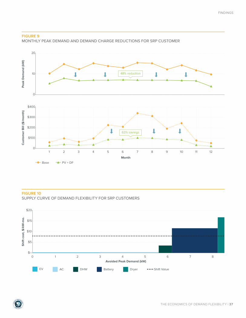
RO

C

KY MOUNTAIN

INSTIT UTE


FINDINGS

FIGURE 10SUPPLY CURVE OF DEMAND FLEXIBILITY FOR SRP CUSTOMERS

FIGURE 9MONTHLY PEAK DEMAND AND DEMAND CHARGE REDUCTIONS FOR SRP CUSTOMER

10

20

0

Pea

k D

eman

d (k

W)

48% reduction

$100

$200

$300

$400

0

Cus

tom

er B

ill ($

/mon

th)

Month

1 2 3 4 5 6 7 8 9 10 11 12

63% savings

Base PV + DF

Monthly Peak and Demand Charges

$15

$20

$5

$10

$–0 1 2 3 4 5 6 7 8

Shi

ft c

ost,

$/k

W-m

o.

Avoided Peak Demand (kW)

AC DryerDHW BatteryEV Shift Value

Supply Curve of Demand Reduction

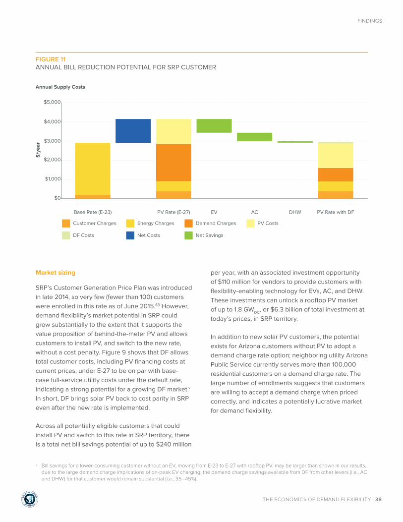
RO

C

KY MOUNTAIN

INSTIT UTE


FINDINGS

Market sizing

SRP’s Customer Generation Price Plan was introduced in late 2014, so very few (fewer than 100) customers were enrolled in this rate as of June 2015.63 However, demand flexibility’s market potential in SRP could grow substantially to the extent that it supports the value proposition of behind-the-meter PV and allows customers to install PV, and switch to the new rate, without a cost penalty. Figure 9 shows that DF allows total customer costs, including PV financing costs at current prices, under E-27 to be on par with base-case full-service utility costs under the default rate, indicating a strong potential for a growing DF market.v In short, DF brings solar PV back to cost parity in SRP even after the new rate is implemented.

Across all potentially eligible customers that could install PV and switch to this rate in SRP territory, there is a total net bill savings potential of up to $240 million

per year, with an associated investment opportunity of $110 million for vendors to provide customers with flexibility-enabling technology for EVs, AC, and DHW. These investments can unlock a rooftop PV market of up to 1.8 GWDC, or $6.3 billion of total investment at today’s prices, in SRP territory.

In addition to new solar PV customers, the potential exists for Arizona customers without PV to adopt a demand charge rate option; neighboring utility Arizona Public Service currently serves more than 100,000 residential customers on a demand charge rate. The large number of enrollments suggests that customers are willing to accept a demand charge when priced correctly, and indicates a potentially lucrative market for demand flexibility.

v Bill savings for a lower-consuming customer without an EV, moving from E-23 to E-27 with rooftop PV, may be larger than shown in our results, due to the large demand charge implications of on-peak EV charging; the demand charge savings available from DF from other levers (i.e., AC and DHW) for that customer would remain substantial (i.e., 35–45%).

FIGURE 11ANNUAL BILL REDUCTION POTENTIAL FOR SRP CUSTOMER

$5,000

$4,000

$3,000

$2,000

$1,000

$0

$/y

ear

Customer Charges Energy Charges Demand Charges

Net Costs Net Savings

PV Costs

DF Costs

Base Rate (E-23) PV Rate (E-27) EV AC DHW PV Rate with DF

Annual Supply Costs

RO

C

KY MOUNTAIN

INSTIT UTE


FINDINGS

SCENARIO 3: NON-EXPORTING ROOFTOP SOLAR PV RATE

Finding: Demand flexibility sustains rooftop solar economics when export compensation is zero

A proposal by the Hawaii Public Service Commission has asked the Hawaiian Electric Company (HECO) to offer a non-export option to new PV customers.64 In a non-export scenario, rooftop PV owners receive no compensation or bill credit for PV energy they export to the grid (i.e., solar PV production has value to the homeowner only if used on-site). For analytic purposes, we maintain HECO’s existing volumetric rate and assume that excess PV is not compensated by the utility; we analyze the economics of DF technologies for a full-service customer considering adding a rooftop PV system under the non-export rate.

We model a relatively large (10 kWAC) PV system because in this case, the economics support large array sizes. This size is also suitable for the relatively high-usage customer (i.e., high AC use plus an electric vehicle) included in this analysis.

TABLE 9SCENARIO-SPECIFIC MODELING SETUP: NON-EXPORTING ROOFTOP SOLAR PV RATE


Utility Hawaiian Electric Company (HECO)

Program name/Rate design DG 2.0 Non-Export Proposal65 (proposed option for new PV customers)

Geography (TMY3 location) Honolulu, HI (Honolulu International Airport)

Customers participating Approximately 270,000 utility customers; 51,000 NEM customers (as of 12/31/2014)

Fixed charges $9.00/month

Demand charges None

Energy charges Inclining block from $0.34–$0.37/kWh; exports earn $0.00/kWh.

Customer PV array size analyzed 10 kWAC (supplies ~80% of household demand)

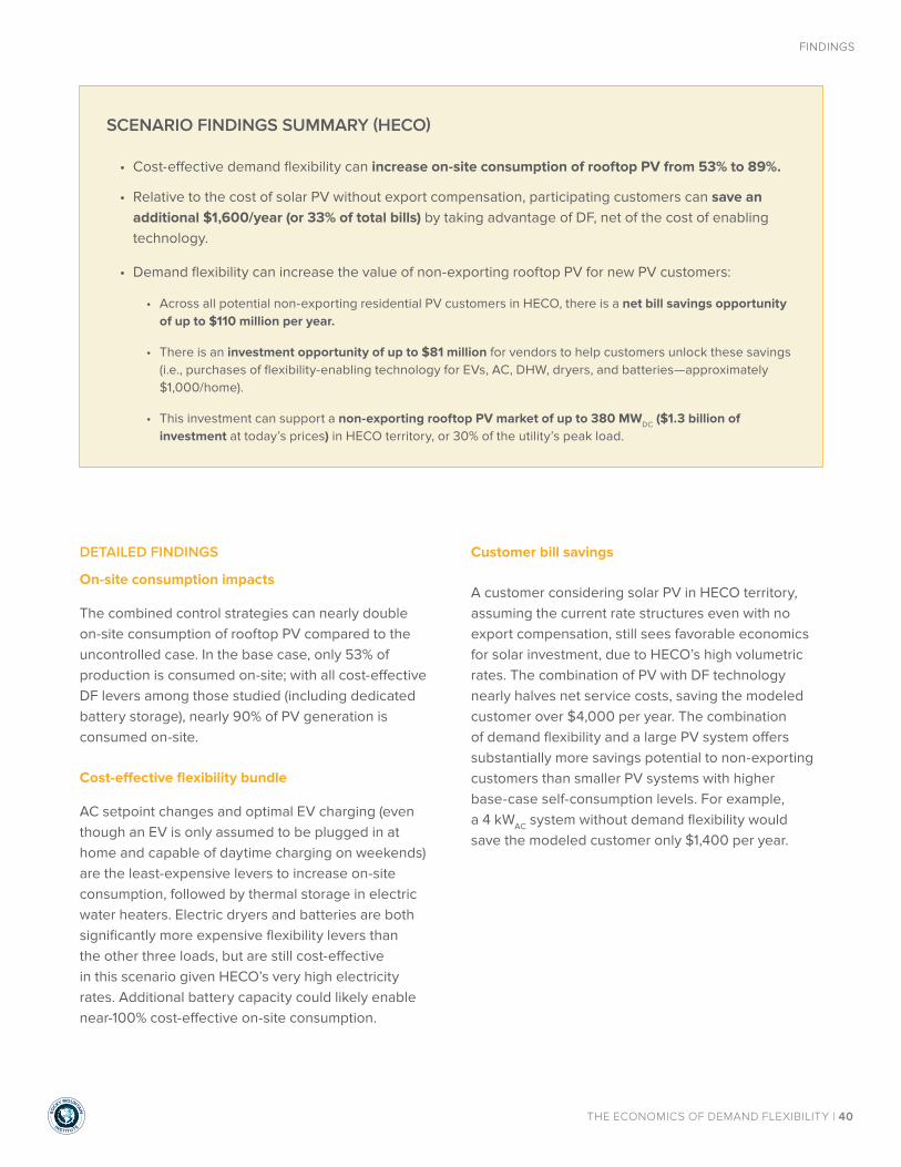
RO

C

KY MOUNTAIN

INSTIT UTE


FINDINGS

DETAILED FINDINGS

On-site consumption impacts

The combined control strategies can nearly double on-site consumption of rooftop PV compared to the uncontrolled case. In the base case, only 53% of production is consumed on-site; with all cost-effective DF levers among those studied (including dedicated battery storage), nearly 90% of PV generation is consumed on-site.


AC setpoint changes and optimal EV charging (even though an EV is only assumed to be plugged in at home and capable of daytime charging on weekends) are the least-expensive levers to increase on-site consumption, followed by thermal storage in electric water heaters. Electric dryers and batteries are both significantly more expensive flexibility levers than the other three loads, but are still cost-effective in this scenario given HECO’s very high electricity rates. Additional battery capacity could likely enable near-100% cost-effective on-site consumption.


A customer considering solar PV in HECO territory, assuming the current rate structures even with no export compensation, still sees favorable economics for solar investment, due to HECO’s high volumetric rates. The combination of PV with DF technology nearly halves net service costs, saving the modeled customer over $4,000 per year. The combination of demand flexibility and a large PV system offers substantially more savings potential to non-exporting customers than smaller PV systems with higher base-case self-consumption levels. For example, a 4 kWAC system without demand flexibility would save the modeled customer only $1,400 per year.

SCENARIO FINDINGS SUMMARY (HECO)

• Cost-effective demand flexibility can increase on-site consumption of rooftop PV from 53% to 89%.

• Relative to the cost of solar PV without export compensation, participating customers can save an additional $1,600/year (or 33% of total bills) by taking advantage of DF, net of the cost of enabling technology.

• Demand flexibility can increase the value of non-exporting rooftop PV for new PV customers:

• Across all potential non-exporting residential PV customers in HECO, there is a net bill savings opportunity of up to $110 million per year.

• There is an investment opportunity of up to $81 million for vendors to help customers unlock these savings (i.e., purchases of flexibility-enabling technology for EVs, AC, DHW, dryers, and batteries—approximately $1,000/home).

• This investment can support a non-exporting rooftop PV market of up to 380 MWDC ($1.3 billion of investment at today’s prices) in HECO territory, or 30% of the utility’s peak load.

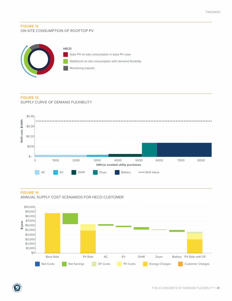
RO

C

KY MOUNTAIN

INSTIT UTE


FINDINGS


FIGURE 12ON-SITE CONSUMPTION OF ROOFTOP PV

HECO

Remaining exports

Solar PV on-site consumption in base PV case

Additional on-site consumption with demand flexibility

On-site Consumption of Rooftop PV

$0.30

$0.40

$0.10

$0.20

$–0 1000 2000 3000 4000 5000 6000 7000 8000

Shi

ft c

ost,

$/k

Wh

kWh/yr avoided utility purchases


Supply Curve of Shifted Energy

FIGURE 14ANNUAL SUPPLY COST SCENARIOS FOR HECO CUSTOMER

$5,000

$6,000

$7,000

$8,000

$9,000

$10,000

$4,000

$3,000$2,000

$1,000

$0

$/y

ear

Customer ChargesEnergy ChargesDF CostsNet Costs PV CostsNet Savings

Base Rate PV Rate AC EV DHW Dryer Battery PV Rate with DF

Annual Supply Costs

RO

C

KY MOUNTAIN

INSTIT UTE


FINDINGS

Market sizing

Depending on the final regulator-approved structure of HECO’s non-export rate option, which is likely to incentivize non-exporting PV systems, demand flexibility could significantly improve PV economics and support even broader adoption of PV in Hawaii. Although HECO already serves nearly 50,000 net-metered customers and will continue to offer a rate option that compensates customers for exported solar in addition to its non-export option, DF may continue to expand the achievable market for new customers, depending on final changes to NEM terms. Additionally, HECO notes that non-export systems will not be subject to an interconnection review study,66 substantially reducing the time from a signed customer contract to an operating PV system.

We find annual net customer bill savings from demand flexibility of up to $110 million per year if all eligible customers in HECO territory install PV under the proposed non-export rate. There is an investment opportunity of up to $81 million to enable these savings, supporting a non-exporting rooftop PV market of up to 380 MWDC, or $1.3 billion of total investment at today’s prices.

RO

C

KY MOUNTAIN

INSTIT UTE


FINDINGS

BOX 4DEMAND FLEXIBILITY HELPS ADDRESS THE PROBLEMS HIGHLIGHTED IN THE “DUCK CURVE”

Utilities and regulators in areas with growing penetration of rooftop PV are beginning to address the “duck curve:” the scenario in which, after system demand is depressed during midday peak solar generation, a rapid ramp-up in generation is required to serve late-afternoon loads as solar PV generation decreases while loads remain high.67

Demand flexibility can play a significant role in mitigating the duck curve. The pairing of rooftop PV and flexible demand with more-granular price signals enables customers to shift consumption away from peak periods and reduce the steep ramping requirement. Among other strategies, this could include pre-heating water, pre-cooling houses, and timing electric vehicle charging to occur during solar PV generation or overnight. Our case analyses for HECO and Alabama Power illustrate the potential for customer loads to shift seamlessly into times of robust solar production.

In this illustration built from our HECO case analysis, a residential customer shifts consumption to the middle of the day, when PV generation peaks, to avoid sharply increasing demand when PV generation declines even as demand remains high. In doing so, both the ramping requirements and the risk of overgeneration (when demand falls below the output of generators that cannot be easily or cost-effectively ramped up and down) are reduced.

FIGURE 15DEMAND FLEXIBILITY AND THE DUCK CURVE

4

3

2

1

-

kW

Load PV Net Load Flexible Net Load

0 4 8 12 16 20 24Hour

4

3

2

1

-0 4 8 12 16 20 24

Hour

RO

C

KY MOUNTAIN

INSTIT UTE


FINDINGS

SCENARIO 4: AVOIDED COST COMPENSATION FOR EXPORTED PV

Finding: Demand flexibility accelerates PV cost parity

Because of avoided cost compensation and mandatory fixed charges, solar PV has poor economics in Alabama Power territory. The utility offers avoided-cost compensation for all exported PV, rather than crediting at the retail rate, and also imposes a non-bypassable capacity charge of $5/kW-month for behind-the-meter generation. We analyze the economics of demand flexibility both for a customer with an existing PV system, and for a full-service customer considering adding a small rooftop PV system.

TABLE 10SCENARIO-SPECIFIC MODELING SETUP: AVOIDED COST EXPORT COMPENSATION


Utility Alabama Power

Program name/Rate design Alabama Power Family Dwelling Residential Service68 and Purchase of Alternative Energy (PAE)69 (mandatory for all PV customers; we modeled PAE Option A for export compensation)

Geography (TMY3 location) Birmingham, AL (Birmingham Municipal Airport)

Customers participating Less than 100 customers currently;70 approximately 1.2 million total utility residential customers

Fixed charges $14.50/month for all residential customers; additional $0.82/month and $5/month per kW of PV capacity for PV customers on rate PAE

Demand charges None

Energy charges $0.111/kWh (first 1,000 kWh); exports earn $0.0316/kWh (June–Sept), $0.0288/kWh (October–May)

Customer PV array size analyzed 4 kWAC (35% of household demand)

RO

C

KY MOUNTAIN

INSTIT UTE


FINDINGS

DETAILED FINDINGS

On-site consumption potential

Only small PV systems approach cost-effectiveness under the rate structure analyzed because of the PV-specific capacity charge. Demand flexibility can increase on-site consumption from small systems from 64% with uncontrolled loads to over 93% with flexible loads—in other words, it virtually eliminates export and turns PV into a behind-the-meter resource.


Demand flexibility from AC and DHW levers are most cost-effective.vi EV charging is also cost-effective but represents a smaller load-shifting potential given the small PV array size. DF-capable dryers and batteries are not cost-effective, largely due to the small PV array size and the resulting limited potential for load-shifting after applying other flexibility levers.


Due to low retail rates and a relatively low capacity factor (18%vii) for PV in Alabama, rooftop PV is barely cost-competitive at our assumed installation prices, even under rate structures that would be favorable to PV, such as NEM or the absence of solar-specific fixed charges. With Alabama Power’s avoided cost export compensation and high solar-specific fees, PV would add significantly to total service costs for a typical customer. However, for a customer with an existing PV system, DF technologies can reduce net utility bills by 11%. For a customer considering adding a new PV system, adding DF reduces the cost penalty of doing so to less than $35/month higher than full-service utility costs. A large fraction of that remaining cost penalty ($20/month) is due to Alabama Power’s specific and non-bypassable capacity charge for PV customers. If a completely non-exporting solar array were found to be exempt from the solar-specific capacity charge, this cost difference would be reduced to $15/month or less.

SCENARIO FINDINGS SUMMARY (APC)

• Cost-effective demand flexibility can increase on-site consumption of rooftop PV from 64% to 93%.

• Relative to the cost of solar PV without export compensation, participating customers can save an additional $210/year (or 11% of total bills) by taking advantage of DF, net of the cost of enabling technology.

• Demand flexibility can accelerate grid parity of rooftop PV by 3–6 years, to 2020 under current rate structures, opening up the market for PV in Alabama. For example, in 2020:

• Across all potential residential PV customers in Alabama Power territory, there is a net bill savings opportunity of up to $210 million per year.

• There is an investment opportunity of up to $230 million for vendors to help customers unlock these savings (i.e., purchases of flexibility-enabling technology for EVs, AC, and DHW—approximately $400/home).

• This investment can support a rooftop PV market of up to 2.9 GWDC ($10 billion of investment at today’s prices)—24% of the utility’s peak demand.

vi Alabama Power offers a $200 rebate for new electric water heaters, negating the incremental cost of adding demand flexibility controls to this appliance.

vii See Appendix B for NREL SAM results.

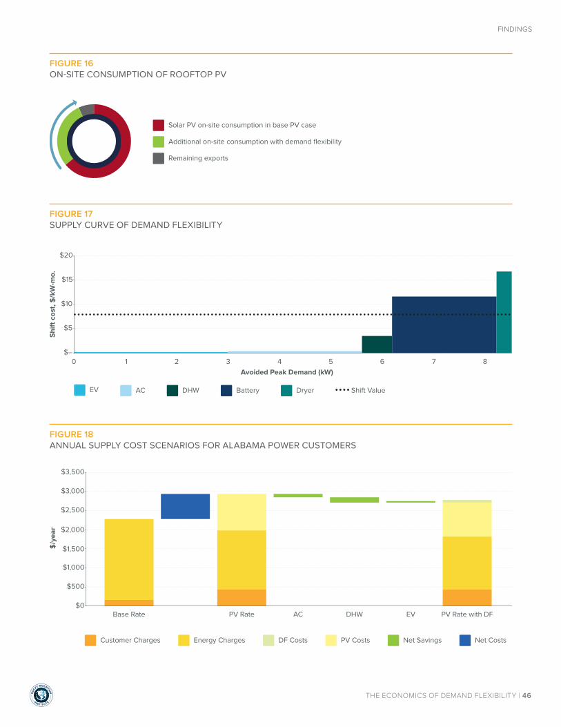
RO

C

KY MOUNTAIN

INSTIT UTE


FINDINGS


FIGURE 16ON-SITE CONSUMPTION OF ROOFTOP PV

Remaining exports

Solar PV on-site consumption in base PV case

Additional on-site consumption with demand flexibility

Self-Consumption of Rooftop PV

$15

$20

$5

$10

$–0 1 2 3 4 5 6 7 8

Shi

ft c

ost,

$/k

W-m

o.

Avoided Peak Demand (kW)


Supply Curve of Demand Reduction

FIGURE 18ANNUAL SUPPLY COST SCENARIOS FOR ALABAMA POWER CUSTOMERS

$2,500

$3,000

$3,500

$2,000

$1,500

$1,000

$500

$0

$/y

ear

Customer Charges Energy Charges DF Costs Net CostsPV Costs Net Savings

Base Rate PV Rate AC DHW EV PV Rate with DF

Annual Supply Costs

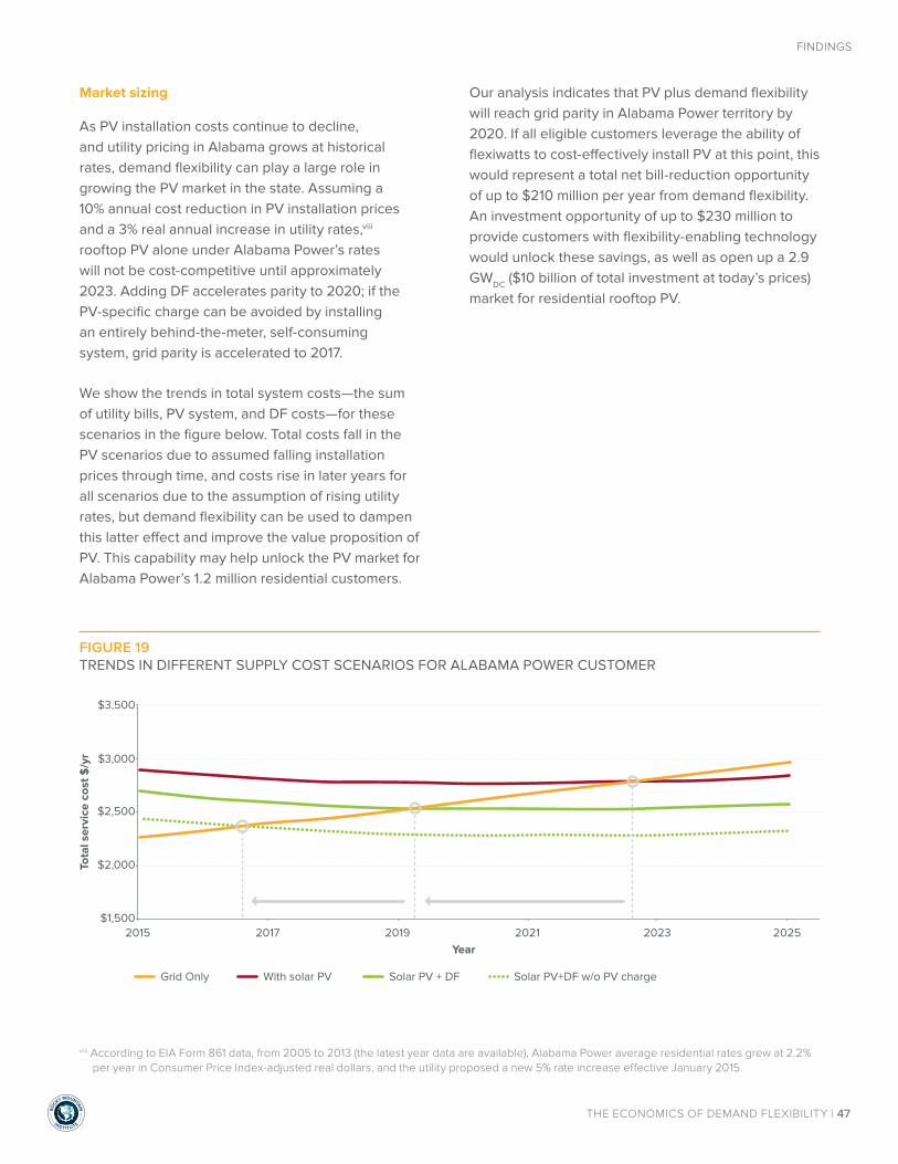
RO

C

KY MOUNTAIN

INSTIT UTE


FINDINGS

Market sizing

As PV installation costs continue to decline, and utility pricing in Alabama grows at historical rates, demand flexibility can play a large role in growing the PV market in the state. Assuming a 10% annual cost reduction in PV installation prices and a 3% real annual increase in utility rates,viii rooftop PV alone under Alabama Power’s rates will not be cost-competitive until approximately 2023. Adding DF accelerates parity to 2020; if the PV-specific charge can be avoided by installing an entirely behind-the-meter, self-consuming system, grid parity is accelerated to 2017.

We show the trends in total system costs—the sum of utility bills, PV system, and DF costs—for these scenarios in the figure below. Total costs fall in the PV scenarios due to assumed falling installation prices through time, and costs rise in later years for all scenarios due to the assumption of rising utility rates, but demand flexibility can be used to dampen this latter effect and improve the value proposition of PV. This capability may help unlock the PV market for Alabama Power’s 1.2 million residential customers.

Our analysis indicates that PV plus demand flexibility will reach grid parity in Alabama Power territory by 2020. If all eligible customers leverage the ability of flexiwatts to cost-effectively install PV at this point, this would represent a total net bill-reduction opportunity of up to $210 million per year from demand flexibility. An investment opportunity of up to $230 million to provide customers with flexibility-enabling technology would unlock these savings, as well as open up a 2.9 GWDC ($10 billion of total investment at today’s prices) market for residential rooftop PV.

FIGURE 19TRENDS IN DIFFERENT SUPPLY COST SCENARIOS FOR ALABAMA POWER CUSTOMER

$3,500

$3,000

$2,500

$2,000

$1,500

Tota

l ser

vice

cos

t $/y

r

Grid Only Solar PV + DF Solar PV+DF w/o PV chargeWith solar PV

2015 2017 2019 2021 2023 2025Year

Trends in Supply Cost Scenarios

viii According to EIA Form 861 data, from 2005 to 2013 (the latest year data are available), Alabama Power average residential rates grew at 2.2% per year in Consumer Price Index-adjusted real dollars, and the utility proposed a new 5% rate increase effective January 2015.

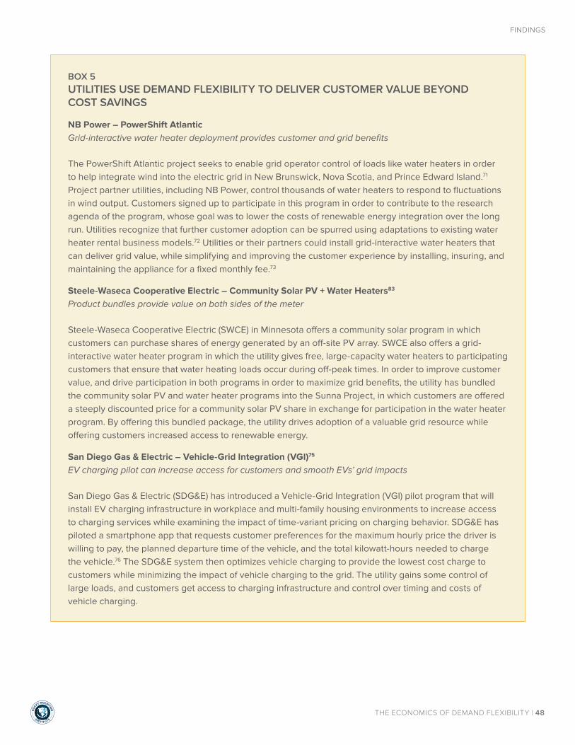
RO

C

KY MOUNTAIN

INSTIT UTE


FINDINGS

BOX 5UTILITIES USE DEMAND FLEXIBILITY TO DELIVER CUSTOMER VALUE BEYOND COST SAVINGS

NB Power – PowerShift Atlantic Grid-interactive water heater deployment provides customer and grid benefits

The PowerShift Atlantic project seeks to enable grid operator control of loads like water heaters in order to help integrate wind into the electric grid in New Brunswick, Nova Scotia, and Prince Edward Island.71 Project partner utilities, including NB Power, control thousands of water heaters to respond to fluctuations in wind output. Customers signed up to participate in this program in order to contribute to the research agenda of the program, whose goal was to lower the costs of renewable energy integration over the long run. Utilities recognize that further customer adoption can be spurred using adaptations to existing water heater rental business models.72 Utilities or their partners could install grid-interactive water heaters that can deliver grid value, while simplifying and improving the customer experience by installing, insuring, and maintaining the appliance for a fixed monthly fee.73

Steele-Waseca Cooperative Electric – Community Solar PV + Water Heaters83

Product bundles provide value on both sides of the meter

Steele-Waseca Cooperative Electric (SWCE) in Minnesota offers a community solar program in which customers can purchase shares of energy generated by an off-site PV array. SWCE also offers a grid-interactive water heater program in which the utility gives free, large-capacity water heaters to participating customers that ensure that water heating loads occur during off-peak times. In order to improve customer value, and drive participation in both programs in order to maximize grid benefits, the utility has bundled the community solar PV and water heater programs into the Sunna Project, in which customers are offered a steeply discounted price for a community solar PV share in exchange for participation in the water heater program. By offering this bundled package, the utility drives adoption of a valuable grid resource while offering customers increased access to renewable energy.

San Diego Gas & Electric – Vehicle-Grid Integration (VGI)75

EV charging pilot can increase access for customers and smooth EVs’ grid impacts

San Diego Gas & Electric (SDG&E) has introduced a Vehicle-Grid Integration (VGI) pilot program that will install EV charging infrastructure in workplace and multi-family housing environments to increase access to charging services while examining the impact of time-variant pricing on charging behavior. SDG&E has piloted a smartphone app that requests customer preferences for the maximum hourly price the driver is willing to pay, the planned departure time of the vehicle, and the total kilowatt-hours needed to charge the vehicle.76 The SDG&E system then optimizes vehicle charging to provide the lowest cost charge to customers while minimizing the impact of vehicle charging to the grid. The utility gains some control of large loads, and customers get access to charging infrastructure and control over timing and costs of vehicle charging.

RO

C

KY MOUNTAIN

INSTIT UTE


FINDINGS

BOX 6ALTERNATIVE SCENARIO: THE ECONOMICS OF LOAD DEFECTION, REVISITED

Finding: Utilities should see demand flexibility as a huge opportunity to reduce grid costs, but under unfavorable rate structures, demand flexibility can instead hasten load defection by accelerating solar PV’s economics in the absence of net energy metering (NEM).

Our April 2015 report The Economics of Load Defection examined the economics of grid-connected solar-plus-battery

storage systems, and found that due to rapidly declining costs, these systems are likely to become cost-competitive

with utility rates in the near future.77 By examining the range of utility rates in the Northeast region of the United

States, we found that solar-plus-battery systems could serve 50% of total regional residential load at an average of

15% below utility prices in 2030, leading to massive “load defection” from utilities and dramatically reducing utility

revenues.

These results hinge upon an emerging theme in utility rate design conversations: how to compensate customers

for behind-the-meter generation (e.g., solar PV) that is exported to the grid. Current net energy metering (NEM)

tariffs are the norm, but several utilities (including Alabama Power) and trade organizations have proposed

compensating exported PV at the avoided cost of energy.78 This simple metric risks undervaluing the true benefits of

distributed PV.79 So how would customers respond, and what would be the implications of a large-scale move to this

compensation mechanism? What if more utilities adopt rate structures to discourage solar PV deployment? Can the

rooftop PV market continue to grow? Are customers gaining competitive tools to defeat utilities’ efforts to discourage

competition from PV systems?

In the load defection analysis, we calculated the potential of batteries to raise on-site consumption of PV energy

in the absence of export compensation (e.g. net energy metering). Here we update that analysis by looking at DF

as a potential lower-cost alternative to dedicated battery storage to improve the value proposition of rooftop PV if

export compensation were reduced or eliminated. We examine the same range of rates in the U.S. Northeast, and

use the same PV cost decline and utility rate increase assumptions as in the load defection analysis. We assume that

export compensation reflects avoided wholesale energy costs, and calculate optimal PV system sizes both with and

without demand flexibility. Under this assumption of a move towards avoided-cost export compensation, we find

that DF increases the total PV market in the Northeast by 60% through 2030, accelerating solar PV economics—and

counteracting the effects of utility rates that limit export compensation.

Demand flexibility helps customers consume more PV output on-site, leading to larger cost-effective PV arrays as well

as more customer demand met by rooftop PV rather than by utility sales. The combination of these two factors greatly

accelerates the load defection potential of rooftop PV. Adding demand flexibility to PV systems in the Northeast

raises the cost-effective load defection potential from 20% of residential load in 2030 with PV alone to nearly 40%

with DF.(box continues)

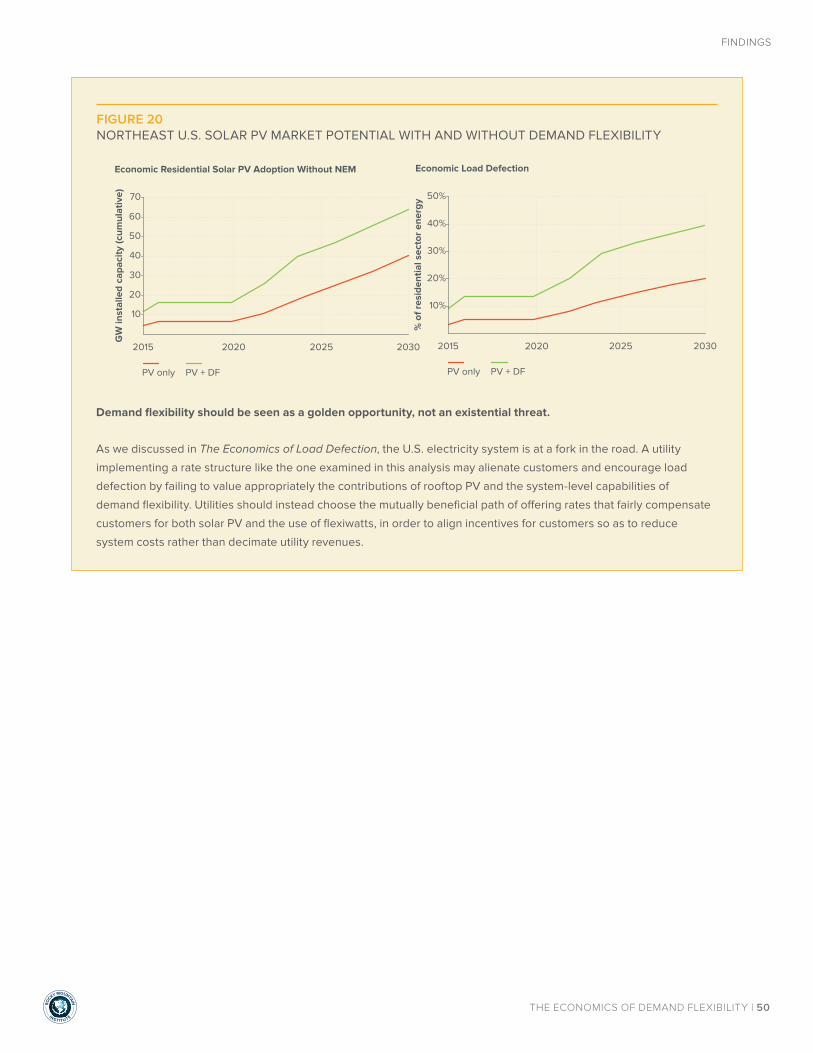
RO

C

KY MOUNTAIN

INSTIT UTE


FINDINGS

Demand flexibility should be seen as a golden opportunity, not an existential threat.

As we discussed in The Economics of Load Defection, the U.S. electricity system is at a fork in the road. A utility

implementing a rate structure like the one examined in this analysis may alienate customers and encourage load

defection by failing to value appropriately the contributions of rooftop PV and the system-level capabilities of

demand flexibility. Utilities should instead choose the mutually beneficial path of offering rates that fairly compensate

customers for both solar PV and the use of flexiwatts, in order to align incentives for customers so as to reduce

system costs rather than decimate utility revenues.

FIGURE 20NORTHEAST U.S. SOLAR PV MARKET POTENTIAL WITH AND WITHOUT DEMAND FLEXIBILITY

20%

40%

30%

10%

50%

2015 2020 2025 2030

% o

f res

iden

tial s

ecto

r en

ergy

Economic Load Defection

PV only PV + DF

20

40

30

10

50

70

60

2015 2020 2025 2030

GW

inst

alle

d ca

paci

ty (c

umul

ativ

e)

Economic Residential Solar PV Adoption Without NEM

PV only PV + DF

IMPLICATIONS AND CONCLUSIONS

04

RO

C

KY MOUNTAIN

INSTIT UTE



DEMAND FLEXIBILITY’S POTENTIAL VALUE MAY BE MUCH LARGER THAN WE ESTIMATE

We have presented the value of demand flexibility in four specific utility cases, both under granular rates that can lead to a more-integrated grid and under assumptions of rates that encourage self-consumption. However, we believe that the total value may greatly exceed the potential estimates presented here for several reasons.

1. We analyze only five levers in the residential sector, but other end-uses, including commercial and industrial loads, can also be made flexible. We do not analyze all residential loads that could be made flexible with evolutions in business models and technology. Moreover, commercial and industrial customers are already largely served by more-granular rates (i.e., time-varying energy pricing and demand charges) that incentivize DF, and solutions are rapidly emerging to capture the savings potential in these buildings (see Box 7).

2. We assume the incremental cost today of flexibility-enabling technology, but that cost could be much lower if integrated into appliances at the factory. For all of the appliance loads we model in this paper, we accounted for the incremental cost to enable communications and control to enable DF. However, these costs could be much lower if DF capabilities were integrated into these appliances at the factory, and not added as a retrofit.

3. There are many more granular rates available to customers than those we analyze in this paper. Approximately 3% of U.S. residential customers—4 million households—already participate in time-varying pricing, and approximately 65 million more have opt-in programs available to them.ix Even given that the majority of these programs are simple time-of-use rates, the DF strategies that we present in this report can be tailored to deliver savings to broad swaths of customers under different rate structures around the country.

4. Demand flexibility technology is already being adopted by a growing number of customers, providing a large existing customer base. Many residential customer segments have already adopted the enabling technology of DF, particularly network-enabled smart thermostats and electric vehicles. To the extent that companies (for example, thermostat manufacturers) can identify and recruit customers to use flexiwatts to reduce bills under existing or new granular rate structures, these customers represent a ready pool of potential savings in utility territories around the country.

While the markets we analyze in this report may be relatively small—hundreds of millions of dollars per year across our four scenarios—compared to the total U.S. market, they represent possible aspects of the near-term future of the grid, for better or for worse. As regulators encourage and utilities pursue well-designed rates to better reflect cost causation and enable massive reductions in grid capacity investments, demand flexibility unlocks a large market for cost reductions. To the extent that rates evolve unfavorably, incentivizing on-site consumption and thus threatening continued PV deployment, DF offers insurance for the rooftop PV market and enhances the value proposition of rooftop PV for customers.


ix EIA Form 861, 2013 (calculated by summing the number of residential customers served by utilities that have customers enrolled in opt-in time-varying rates).

RO

C

KY MOUNTAIN

INSTIT UTE


FINDINGS

BOX 7COMMERCIAL AND INDUSTRIAL SECTOR DEMAND FLEXIBILITY

Many commercial building and industrial facility solutions for demand flexibility already exist. Commercial buildings in most utility territories face demand charges, which can account for a substantial portion of a building’s monthly bill, and can be addressed directly by flexiwatts and/or storage technologies. Below, we outline four distinct strategies, commercially available today, to manage demand charges, optimize for time-varying energy prices, and improve control and visibility of large loads in commercial buildings.

COOLING ENERGY FLEXIBILITYX

Use case: Large commercial buildings with central space cooling facilities (e.g., office towers)

Loads under control: Central chiller plants and other space-cooling equipment

Approach: Software that couples calibrated industry-standard building energy models with advanced optimization methods (e.g., model predictive control) can leverage the thermal mass of large buildings to optimize energy consumption throughout the day. This can reduce both total energy used as well as peak afternoon demand by optimizing zone setpoint schedules against utility rate components (e.g., time-varying energy charges, monthly peak demand charges).

Cost structure: The approach requires no investment in different cooling equipment to achieve savings. Software setup costs for initializing modeling and optimization frameworks, on the order of $30,000 per controlled building, are fixed. Ongoing support, tuning, and maintenance are small, and marginal costs per building at scale are minimal.

Savings potential: Depending on specific utility rate structures, both peak demand and on-peak energy use can be reduced by up to 30% with minimal changes in occupant comfort. Importantly, this strategy can also reduce total energy use, including off-peak energy, by optimizing cooling schedules against equipment performance curves and ambient temperatures.

QUEUED POWER ACCESSXI

Use case: Buildings with multiple motors and/or cycling loads (e.g., retail and telecom small data centers)

Loads under control: Individual loads behind the meter (e.g., HVAC, refrigeration, electric motors, pumps, battery charging, etc.)

Approach: This solution relies on enforcing a non-disruptive queue for power demands—an approach similar to one used in the IT and telecommunications industries to manage network bandwidth. The service queues the operation of individual loads, shifting a small percentage (e.g., 4%) of energy use in order to reduce peak demand. In practical applications for HVAC loads, this approach schedules a compressor’s startup time within 300-second time slots, causing no perceivable impact on end-use quality of service.

Cost structure: If there are no building automation systems (BAS) in place, the communications hardware required can range from $2,000–3,000 per facility. If an open standards BAS is in place, software integration, commissioning and setup costs range from $20,000 to $75,000 depending on BAS scale and facility complexity. Ongoing software service fees are as low as $0.005/kWh.

x See, for example, QCoefficient

xi Queued Power Access is a trademark of eCurv, Inc.

(box continues)

RO

C

KY MOUNTAIN

INSTIT UTE


FINDINGS

(continued)

Savings potential: Queuing access to a shared power supply can achieve peak demand reductions of up to 40%, up to 13% total energy savings, and additional benefits including built-in load monitoring to identify equipment performance issues. Depending on specific utility rate structures, total annual energy bill savings range from 11% to 27% per building.

SMART LIGHTING CONTROLSXII

Use case: Commercial and industrial facilities with large and/or complex lighting control systems (e.g., office buildings, warehouses)

Loads under control: Individual lighting fixtures

Approach: Installation of networked controls for lighting systems allows fine-tuning of lighting fixture output according to occupant presence and preference, real-time daylighting availability, and code-specified minimum output levels. Dimmable fixtures and advanced controls can also contribute substantially to energy and peak demand savings for buildings with high lighting requirements.

Cost structure: Control hardware cost requirements are on the order of $1,000–$3,000 per facility. Costs for efficient lighting hardware (e.g., dimmable LED fixtures) are additional and scale with facility size, but offer rapid payback in energy savings.

Savings potential: Peak demand reductions on the order of 10–20% are achievable depending on building type, load profile, and usage pattern. There are also substantial reductions in total lighting energy usage as well as improvements in lighting quality and flexibility to meet occupant preferences.

BATTERY STORAGEUse case: Any commercial building

Loads under control: Dedicated battery energy storage hardware

Approach: Predictive analytics software coupled with power electronics can optimize the charging and discharging profile of dedicated, behind-the-meter battery systems in order to minimize peak demand levels for large facilities. Peak demand of any type of load can be minimized by battery systems of the appropriate size.

Cost structure: Hardware cost requirements are currently on the order of $350/kWh or less for commercial building battery systems.

Savings potential: Each kW of battery storage capacity has the potential to reduce 1 kW of peak demand and eliminate the associated monthly peak demand charges. Battery systems can also shift on-peak energy to cheaper off-peak hours for buildings with time-varying energy rates; however, there are energy losses on the order of 15–20% due to inverter inefficiency.

xii See, for example, EdgePower

RO

C

KY MOUNTAIN

INSTIT UTE



RATE DESIGN CAN UNLOCK FAR MORE OF DEMAND FLEXIBILITY’S POTENTIAL VALUE

Our analysis suggests that the fundamental economics of demand flexibility are favorable, but many barriers remain to be overcome by regulators, utilities, and third-party innovators in order to capture this value. Of particular importance, to promote the adoption of demand flexibility and line up incentives for customers to help reduce system costs, the design of rates should include four key features:80

1. Increased granularity: to the extent possible, residential rate design should unbundle components of usage (e.g., energy, capacity, ancillary services) and add temporal (e.g., peak / off-peak energy and capacity) and locational components.

2. Technology agnostic: rates should not prefer or discriminate against specific technologies and instead be designed to charge and compensate customers at prices that reflect marginal costs for services consumed and provided.

3. Expand customer choice: customers should not be constrained to one rate option designed to reflect the cost causation of an “average” customer. Customers should be able to opt in to rate structures of varying granularity according to their preferences and the availability of technology to enable cost reductions.

4. New default options: utilities typically have multiple rate options for residential customers, and almost universally, the default option is the volumetric energy charge with no temporal variation or attribute unbundling. New default options can help unlock the value of demand flexibility for many more customers than are currently enrolled in opt-in granular rate structures.81

STAKEHOLDER IMPLICATIONS

Innovation within the U.S. electricity system today is in a holding pattern, as emerging technologies and capabilities confront a system built on twentieth- or even nineteenth-century paradigms. Every stakeholder needs to act on the incentives that exist today. To capture the benefits of demand flexibility for customers and the system at large, three key stakeholder groups need to work together to arrive at a higher-quality, lower-cost outcome: third-party innovators, utilities, and state regulators. Only through coordinated action can we shift from the current state—which works well but at a higher than necessary cost—to one that uses all available levers to run the system more efficiently.

Third-party innovators already have the technology and business models to capture the value of flexiwatts (and the scenarios covered in this paper highlight real opportunities to do so today) but are limited in scale by a lack of granular rates or local market participation options available from many utilities. Utilities in many cases need regulatory support and incentives to introduce rates that would enable DF to reduce system costs. State regulators can encourage rates that scale demand flexibility, but need to see demonstrated capacity from innovators to ensure that customers can respond in ways that successfully reduce system costs. In this way, unilateral action by any of the stakeholders is challenging.

Scaling demand flexibility and moving the grid to a lower-cost solution requires concerted and coordinated action around a common goal: to fully harness the value of flexible demand to address grid and customer challenges. We lay out key actions below for each stakeholder group, but the ability to capture the value of flexiwatts at scale will ultimately rely on the success of integrated efforts to find win-win-win value propositions for customers, utilities, and third-party service providers alike.

RO

C

KY MOUNTAIN

INSTIT UTE



THIRD-PARTY INNOVATORS: PURSUE OPPORTUNITIES NOW TO HONE CUSTOMER VALUE PROPOSITION

Many different kinds of companies can capture the value of flexiwatts, including home energy management system providers, solar PV developers, demand response companies, and appliance manufacturers, among others. These innovators can take the following actions to capitalize on the DF opportunity:

Take advantage of opportunities that exist today

Low-cost, high-capability technology to achieve demand flexibility is available today; scaling the market requires merging this technology with business models that seamlessly deliver customer value. Forty million customers today have access to opt-in granular rates; innovators can empower these customers to save money on their bills by providing products and services that complement or compete with traditional, bundled utility energy sales. The scenarios discussed in this paper illustrate the range of present-day opportunities for developers to do so; these scenarios represent an opportunity to refine the customer value proposition and test a variety of solutions that can allow these business models to scale in the future.

Offer customers more than just bill savings

Granular rates and demand flexibility can offer direct bill savings, but other drivers of customer demand have been proven to be potentially more important. Similar to efficiency—where many retrofits are driven by improved comfort or resale value, with bill savings as a secondary value—DF’s ability to improve the customer experience might be a bigger draw than savings alone.

Companies can use DF to enhance proven strategies for different customer segments:

• The potential to offer DF bundles that deliver bill savings along with desirable consumer products (e.g., smart thermostats, rooftop PV, electric vehicles) may offer a ready customer base and cross-marketing opportunities for third-party providers. To broaden the market even further, look for opportunities to find low-cost, streamlined solutions for lower-income, lower-usage customer groups.

• Offer better, not just cheaper, services with demand flexibility-enabled products by streamlining maintenance and upkeep of appliances (e.g., water heating,82 air conditioning ).83

• Several companies have built successful load management programs for certain customer segments using targeted behavioral messaging (e.g., utility bill inserts that include comparisons to average neighborhood bills);84 adding DF technology may offer the opportunity to enhance these programs.

• Many customers make investment decisions for appliances based on first cost alone. Companies can pursue strategies to make DF-enabled appliances the least cost option a potential buyer sees when making purchase decisions. An example is offering rebates on appliances whose costs can be covered by a shared savings model with the customer over the life of the appliance.

• Just as major home appliances already have Energy Star ratings and stickers indicating the annual cost to operate, DF-capable appliances can similarly carry a flexibility rating. These ratings could indicate the added annual value that demand flexibility offers customers who choose to tap into it, and would send a potentially powerful signal to consumers about the explicit monetary value of demand flexibility.

RO

C

KY MOUNTAIN

INSTIT UTE



Pursue standardized and secure technology, integrated at the factory

Standardization and interoperability are vital for DF solutions to achieve scale and deliver grid and customer value.85 Many solutions exist to allow low-cost integration of communications and control technology at the time of manufacture;86 by incorporating standardized technology by default for consumer appliances, and not as a retrofit, upfront costs for flexibility can fall precipitously and widen the available market. Developers should also consider customer privacy and security in developing software and communication protocols to support flexibility, in order to mitigate some stakeholders’ concerns around adoption of networked, flexible loads; close, early, and universal attention to security is essential in order to avoid highly publicized mishaps that give demand flexibility a bad name.

Find partnerships to monetize demand flexibility in front of the meter

Once companies have achieved sufficient scale in a utility service territory with customer-facing models, they can seek out additional opportunities to integrate programs that deliver further grid value (e.g., reduced peak capacity needs, renewable integration, etc.), in partnership with host utilities or other service providers. Traditional demand response models have been slow to scale, but by finding innovative ways to get demand flexibility into customer homes, companies can combine customer value with grid value to grow revenue and reduce system costs.

UTILITIES: LEVERAGE WELL-DESIGNED RATES TO REDUCE GRID COSTS

Utilities of all types—vertically-integrated, wires-only, retail providers, etc.—can capture DF’s grid value by taking the following steps:

Introduce and promote rates that reflect marginal costs

By offering enabling rate options that allow customers to respond to granular pricing according to their preferences and technological ability, utilities can help customers lower their bills while reducing grid costs. On the other hand, if rates offer no customer incentive to reduce grid costs (e.g., high fixed charges, uneconomic on-site consumption incentives, poorly designed demand charges), DF may instead empower and encourage customers to reduce their bills (i.e., reduce utility revenue) without creating a commensurate drop in utility costs. This could provide customers major benefits from PV and other DERs, while depriving utilities of the benefits of flexiwatts they could otherwise capture.

Consider flexiwatts as a resource, not a threat

While our analysis focuses on the customer economics of demand flexibility, as a resource deployed at scale it has massive potential to reshape load profiles to reduce peak loads, avoid high-price energy production, and integrate renewable energy. Having flexible demand as well as flexible supply is a fundamentally better and smarter way to run a network—flexiwatts can be as effective as generation capacity in meeting many grid needs. Utilities should consider demand flexibility a resource, not a threat, and figure out how to harness it. Treating flexiwatts, PV, and other DERs as threats through unfavorable rate design may be a self-fulfilling prophecy.

Harness the potential of enabling technology and third-party innovation

Utilities can maintain a simpler customer experience despite increasing rate complexity by coupling granular rates with seamless, automated technology and third-party, customer-facing business models. As discussed above, third-party innovators can provide products and services that deliver flexiwatts alongside other desirable customer outcomes; these solutions coupled with granular rates can help utilities ensure that new rates address system cost concerns.

RO

C

KY MOUNTAIN

INSTIT UTE



REGULATORS: PROMOTE FLEXIWATTS AS A LEAST-COST SOLUTION TO GRID CHALLENGES

In order to ensure that demand flexibility reaches its full potential to reduce system costs, and that third-party innovation can empower customers to reduce their bills, state regulators have a role to play in encouraging utilities to promote and fully value flexiwatts as a low-cost resource. Regulators should consider the following:

Recognize the cost advantage of demand flexibility

Regulators should recognize the power of innovation to deliver DF at very low cost compared to traditional infrastructure investments. Some infrastructure investments are likely prudent to ensure system reliability, but investments in DF should be considered as a lower-cost alternative when and where appropriate. Third-party business models that harness DF can deliver many sources of value to customers; by letting the customer value proposition drive the adoption of flexibility, the net cost to the grid to offset traditional investment can be very low. To the extent that grid-level technology may be required to enable demand flexibility (e.g., advanced metering infrastructure (AMI)), regulators can help enable their wide adoption, while recognizing that there are many available options to achieve different communications and control goals (e.g., internet-connected home energy management systems, smart inverters, etc.) that may not require significant upfront investment.

Encourage utilities to offer a variety of rates to promote customer choice

Demand flexibility’s ability to provide value to the grid and reduce system costs rests on a foundation of well-designed granular rates. Though there are many customers who have the option to participate in granular rates today, these rates still need to reach wider adoption (and likely some increase in granularity) in order to capture the grid cost savings of the magnitude discussed in our analysis. Regulators should balance the potential complexity of highly granular rates against the attractive value proposition for customers and the grid. A growing body of evidence suggests defaulting customers to more granular rates can provide both savings and a positive customer experience.87 However, maintaining the availability of less granular,

more traditional block, volumetric rates can help to ensure that customers without the ability or interest to adopt new technologies can maintain a simple customer experience.

Encourage utilities to innovate and seek partnerships to harness demand flexibility

In order to capture the cost advantage of flexiwatts, regulators should encourage utilities to embrace the potential of granular rates, seamless technology, and innovative, customer-facing business models that help customers respond to price signals that reflect system costs. Regulators should recognize that these customer-facing solutions might come from utilities themselves, but often third parties can offer customers a broader variety of innovative solutions. Regulators should encourage utilities to embrace this, and offer rates that allow customers to save money and reduce grid costs by adopting competitive third-party services.

APPENDIX A

ESTIMATING DEMAND FLEXIBILITY GRID VALUE

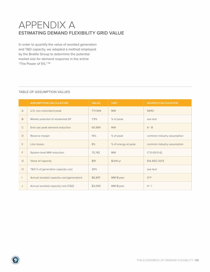
RO

C

KY MOUNTAIN

INSTIT UTE


APPENDIX AESTIMATING DEMAND FLEXIBILITY GRID VALUE

In order to quantify the value of avoided generation and T&D capacity, we adapted a method employed by the Brattle Group to determine the potential market size for demand response in the article “The Power of 5%.” 88

TABLE OF ASSUMPTION VALUES

ASSUMPTION/CALCULATION VALUE UNIT SOURCE/CALCULATION

A U.S. non-coincident peak 771,944 MW NERC

B Market potential of residential DF 7.9% % of peak see text

C End-use peak demand reduction 60,984 MW A * B

D Reserve margin 15% % of peak common industry assumption

E Line losses 8% % of energy at peak common industry assumption

F System-level MW reduction 75,742 MW C*(1+D)*(1+E)

G Value of capacity $91 $/kW-yr EIA AEO 2013

H T&D % of generation capacity cost 30% see text

I Annual avoided capacity cost (generation) $6,897 MM $/year G*F

J Annual avoided capacity cost (T&D) $2,069 MM $/year H * I

RO

C

KY MOUNTAIN

INSTIT UTE


APPENDIX A

We began with the 2014 total U.S. non-coincident peak demand forecast of 771,944 MW.89 To estimate the market potential of demand flexibility, we combined estimates for the total capacity of electric water heaters and air conditioning in the U.S.90 For water heaters, using the NEEA end-use demand database we estimate that each unit has 5 kW of peak demand capacity, but that only 5.5% of connected water heater load is peak coincident (i.e., occurs between 2–8 p.m., June–September), to represent 1.6% of total U.S. peak load.

Air conditioning peak was calculated using FERC data from the 2009 A National Assessment of Demand Response Potential on residential demand and air conditioning saturation and peak demand.91 For each state, we use FERC data for the number of residential customers, the average peak coincident residential demand, and AC saturation. We assume that during peak events where demand flexibility can be used to reduce system load, houses with AC units can shed 25% of total load.xiii Using this assumption along with the FERC data, we estimate a total reduction potential of 48.8 GW during peak events, or 6.3% of U.S. peak load.

We multiply the total savings potential (7.9%) by coincident peak demand, and adjust based on line losses and reserve margins to find the total capacity that can be avoided through reductions in peak end-use demand. We multiply this value by a conservative estimate of avoided costs for generation capacity, and add a similarly conservative avoided cost for transmission and distribution capacity, to arrive at the total avoided capacity costs of $9 billion per year.xiv

We calculated the value of LMP (locational marginal price) arbitrage using demand flexibility from DHW, AC, and electric dryers by analyzing the performance of each load in shifting energy from high-price to low-price hours using 2014 historical hourly price data from each of the seven organized energy markets in the United States.xv We take the average value of these savings, in dollars saved per MWh of end-use load, and scale to total end-use loads for each appliance using EIA RECS 2009 data, to arrive at the total energy cost savings of $3.3 billion per yr.

Contemporary research and pilot projects demonstrate that aggregated residential loads (including AC, DHW, and refrigerators) are technically capable of providing ancillary services to the grid, specifically frequency regulation and spinning reserve, in amounts far greater than needed.92 We estimate the total U.S. market size for providing ancillary services using recent market survey data,93 and scale the market size for the reported regions (CAISO, MISO, ERCOT, and PJM) using their respective fractions of total energy demand. We arrive at estimated market sizes of $710 million per year and $480 million per year for frequency regulation and spinning reserve, respectively.

These values represent the total potential avoided cost for capacity, energy, and ancillary services (frequency regulations and spinning reserve). Our analysis shows that implementing demand flexibility at scale can avoid these costs; however, these numbers do not incorporate the technology and/or program costs of demand flexibility, and thus do not represent the net benefits.

xiv Consistent with our model of A/C flexibility as well as an industry assessment of residential DR programs. For example, Freeman Sullivan Co.’s “2012 Load Impact Evaluation for Pacific Gas & Electric Company’s SmartAC Program” found average savings of 24% for 2011 and 2012 events.

xv Data from Brattle, the California Public Utilities Commission, CAISO, EIA, PJM, Crossborder Energy, and Freeman, Sullivan and Co. reveal generation capacity values to range between $40/kW-year and $190.10/kW-year; we use the EIA’s value of $91/kW-year. Transmission and distribution capacity savings range from $14/kW-year to $57.03/kW-year for distribution and $19.58/kW-year to $65.14/kW-year for transmission; we use a combined total of $27.3/kW-year.

xvi We use the energy component of LMP from each market, if available, to remove the impacts of transmission constraints and congestion. Where not available, we take a simple average across price zones or nodes within the market to estimate the system energy value.

APPENDIX B

DATA SOURCES AND ANALYSIS METHODOLOGY

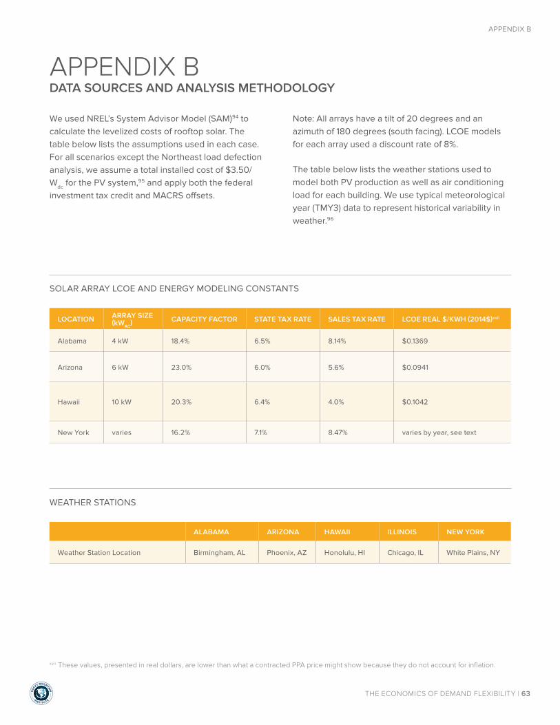
RO

C

KY MOUNTAIN

INSTIT UTE


APPENDIX B

APPENDIX BDATA SOURCES AND ANALYSIS METHODOLOGY

LOCATION ARRAY SIZE (kWAC) CAPACITY FACTOR STATE TAX RATE SALES TAX RATE LCOE REAL $/KWH (2014$)xvii

Alabama 4 kW 18.4% 6.5% 8.14% $0.1369

Arizona 6 kW 23.0% 6.0% 5.6% $0.0941

Hawaii 10 kW 20.3% 6.4% 4.0% $0.1042

New York varies 16.2% 7.1% 8.47% varies by year, see text

ALABAMA ARIZONA HAWAII ILLINOIS NEW YORK

Weather Station Location Birmingham, AL Phoenix, AZ Honolulu, HI Chicago, IL White Plains, NY

xvii These values, presented in real dollars, are lower than what a contracted PPA price might show because they do not account for inflation.

SOLAR ARRAY LCOE AND ENERGY MODELING CONSTANTS

WEATHER STATIONS

We used NREL’s System Advisor Model (SAM)94 to calculate the levelized costs of rooftop solar. The table below lists the assumptions used in each case. For all scenarios except the Northeast load defection analysis, we assume a total installed cost of $3.50/Wdc for the PV system,95 and apply both the federal investment tax credit and MACRS offsets.

Note: All arrays have a tilt of 20 degrees and an azimuth of 180 degrees (south facing). LCOE models for each array used a discount rate of 8%.

The table below lists the weather stations used to model both PV production as well as air conditioning load for each building. We use typical meteorological year (TMY3) data to represent historical variability in weather.96

RO

C

KY MOUNTAIN

INSTIT UTE


APPENDIX B

LOAD MODELING

This section describes the energy data we use as well as the assumptions we make and the control strategies we use in order to model load flexibility for the five flexibility levers we analyze.

We use customized home energy models for each of our five U.S. regions. We modeled baseline customer usage behavior using select 15-minute submetered home energy data from the Northwest Energy Efficiency Alliance (NEEA),97 collected between 2012 and 2013. We used this data to derive typical profiles for behavior-driven appliance use (hot water and electric dryers), as well as to derive estimates for non-flexible load in a typical home (e.g., television, cooking, lights, etc.). We chose one representative house with complete data that was closest to the median energy consumption for each flexible load, for all the homes in the data set. We then removed air conditioning and heating loads from the data set and added in our region-dependent base case air conditioning model to create the base case electric demand.

FLEXIBILITY MODELING METHODOLOGIES

The modeling approach for each flexible load is to shift kWh of electricity demand from high cost times to low cost times, where “cost” depends on the specifics of each modeled scenario (see below for specific modeling approaches used for each appliance in each location). We model load flexibility for each appliance over a full year in 15 minute increments in order to capture the impacts of changing weather, changing energy consumption, and changing solar production on load flexibility value.

Each flexible load has different constraints and operating requirements. Therefore we customize our approach for each appliance in order to optimize its electricity consumption. We detail each appliance’s methodology and assumptions below.

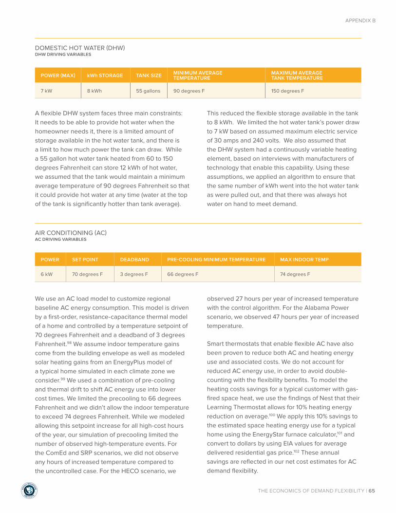
RO

C

KY MOUNTAIN

INSTIT UTE


APPENDIX B

POWER (MAX) kWh STORAGE TANK SIZE MINIMUM AVERAGE TEMPERATURE

MAXIMUM AVERAGE TANK TEMPERATURE

7 kW 8 kWh 55 gallons 90 degrees F 150 degrees F

POWER SET POINT DEADBAND PRE-COOLING MINIMUM TEMPERATURE MAX INDOOR TEMP

6 kW 70 degrees F 3 degrees F 66 degrees F 74 degrees F

DOMESTIC HOT WATER (DHW)DHW DRIVING VARIABLES

AIR CONDITIONING (AC)AC DRIVING VARIABLES

A flexible DHW system faces three main constraints: It needs to be able to provide hot water when the homeowner needs it, there is a limited amount of storage available in the hot water tank, and there is a limit to how much power the tank can draw. While a 55 gallon hot water tank heated from 60 to 150 degrees Fahrenheit can store 12 kWh of hot water, we assumed that the tank would maintain a minimum average temperature of 90 degrees Fahrenheit so that it could provide hot water at any time (water at the top of the tank is significantly hotter than tank average).

This reduced the flexible storage available in the tank to 8 kWh. We limited the hot water tank’s power draw to 7 kW based on assumed maximum electric service of 30 amps and 240 volts. We also assumed that the DHW system had a continuously variable heating element, based on interviews with manufacturers of technology that enable this capability. Using these assumptions, we applied an algorithm to ensure that the same number of kWh went into the hot water tank as were pulled out, and that there was always hot water on hand to meet demand.

We use an AC load model to customize regional baseline AC energy consumption. This model is driven by a first-order, resistance-capacitance thermal model of a home and controlled by a temperature setpoint of 70 degrees Fahrenheit and a deadband of 3 degrees Fahrenheit.98 We assume indoor temperature gains come from the building envelope as well as modeled solar heating gains from an EnergyPlus model of a typical home simulated in each climate zone we consider.99 We used a combination of pre-cooling and thermal drift to shift AC energy use into lower cost times. We limited the precooling to 66 degrees Fahrenheit and we didn’t allow the indoor temperature to exceed 74 degrees Fahrenheit. While we modeled allowing this setpoint increase for all high-cost hours of the year, our simulation of precooling limited the number of observed high-temperature events. For the ComEd and SRP scenarios, we did not observe any hours of increased temperature compared to the uncontrolled case. For the HECO scenario, we

observed 27 hours per year of increased temperature with the control algorithm. For the Alabama Power scenario, we observed 47 hours per year of increased temperature.

Smart thermostats that enable flexible AC have also been proven to reduce both AC and heating energy use and associated costs. We do not account for reduced AC energy use, in order to avoid double-counting with the flexibility benefits. To model the heating costs savings for a typical customer with gas-fired space heat, we use the findings of Nest that their Learning Thermostat allows for 10% heating energy reduction on average.100 We apply this 10% savings to the estimated space heating energy use for a typical home using the EnergyStar furnace calculator,101 and convert to dollars by using EIA values for average delivered residential gas price.102 These annual savings are reflected in our net cost estimates for AC demand flexibility.

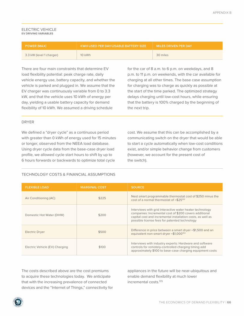
RO

C

KY MOUNTAIN

INSTIT UTE


APPENDIX B

DRYER

TECHNOLOGY COSTS & FINANCIAL ASSUMPTIONS

There are four main constraints that determine EV load flexibility potential: peak charge rate, daily vehicle energy use, battery capacity, and whether the vehicle is parked and plugged in. We assume that the EV charger was continuously variable from 0 to 3.3 kW, and that the vehicle uses 10 kWh of energy per day, yielding a usable battery capacity for demand flexibility of 10 kWh. We assumed a driving schedule

for the car of 8 a.m. to 6 p.m. on weekdays, and 8 p.m. to 11 p.m. on weekends, with the car available for charging at all other times. The base case assumption for charging was to charge as quickly as possible at the start of the time parked. The optimized strategy delays charging until low-cost hours, while ensuring that the battery is 100% charged by the beginning of the next trip.

The costs described above are the cost premiums to acquire these technologies today. We anticipate that with the increasing prevalence of connected devices and the “Internet of Things,” connectivity for

appliances in the future will be near-ubiquitous and enable demand flexibility at much lower incremental costs.105

We defined a “dryer cycle” as a continuous period with greater than 0 kWh of energy used for 15 minutes or longer, observed from the NEEA load database. Using dryer cycle data from the base-case dryer load profile, we allowed cycle start hours to shift by up to 6 hours forwards or backwards to optimize total cycle

cost. We assume that this can be accomplished by a communicating switch on the dryer that would be able to start a cycle automatically when low-cost conditions exist, and/or simple behavior change from customers (however, we account for the present cost of the switch).

POWER (MAX) KWH USED PER DAY/USABLE BATTERY SIZE MILES DRIVEN PER DAY

3.3 kW (level 1 charger) 10 kWh 30 miles

FLEXIBLE LOAD MARGINAL COST SOURCE

Air Conditioning (AC) $225 Nest smart programmable thermostat cost of $250 minus the cost of a normal thermostat of ~$25103

Domestic Hot Water (DHW) $200

Interviews with grid interactive water heater technology companies: Incremental cost of $200 covers additional capital cost and incremental installation costs, as well as possible license fees for patented technology

Electric Dryer $500 Difference in price between a smart dryer ~$1,500 and an equivalent non-smart dryer ~$1,000104

Electric Vehicle (EV) Charging $100Interviews with industry experts: Hardware and software controls for remotely-controlled charging timing add approximately $100 to base-case charging equipment costs

ELECTRIC VEHICLEEV DRIVING VARIABLES

APPENDIX C

SCENARIO-SPECIFIC ASSUMPTIONS AND RESULTS

RO

C

KY MOUNTAIN

INSTIT UTE


APPENDIX C

APPENDIX CSCENARIO-SPECIFIC ASSUMPTIONS AND RESULTS

The table below shows the data underlying the supply curves in the main text.

SCENARIO LEVER SHIFT COST $/kWh OR $/kW-MO SHIFTED kWh OR AVOIDED kW-MO

ComEd AC -$0.11/kWh 191 kWh

DHW $0.02/kWh 1164 kWh

Dryer $0.20/kWh 330 kWh

EV $0.01/kWh 2061 kWh

Battery $0.25/kWh 2079 kWh

SRP AC $0.41/kW-mo 2.6 kW-mo

DHW $3.60/kW-mo 0.6 kW-mo

Dryer $16.76/kW-mo 0.32 kW-mo

EV $0.36/kW-mo 2.98 kW-mo

Battery $10.03/kW-mo 2.0 kW-mo

HECO AC $0.02/kWh 1640 kWh



EV $0.02/kWh 707 kWh


Alabama Power AC -$0.17/kWh 338 kWh



EV $0.05/kWh 250 kWh


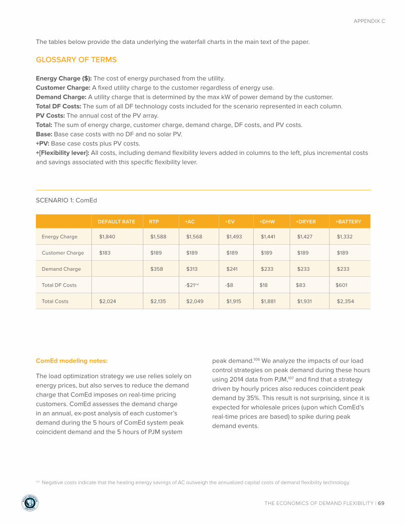
RO

C

KY MOUNTAIN

INSTIT UTE


APPENDIX C

SCENARIO 1: ComEd

The tables below provide the data underlying the waterfall charts in the main text of the paper.

GLOSSARY OF TERMS

Energy Charge ($): The cost of energy purchased from the utility. Customer Charge: A fixed utility charge to the customer regardless of energy use. Demand Charge: A utility charge that is determined by the max kW of power demand by the customer. Total DF Costs: The sum of all DF technology costs included for the scenario represented in each column. PV Costs: The annual cost of the PV array. Total: The sum of energy charge, customer charge, demand charge, DF costs, and PV costs. Base: Base case costs with no DF and no solar PV. +PV: Base case costs plus PV costs. +[Flexibility lever]: All costs, including demand flexibility levers added in columns to the left, plus incremental costs and savings associated with this specific flexibility lever.

ComEd modeling notes:

The load optimization strategy we use relies solely on energy prices, but also serves to reduce the demand charge that ComEd imposes on real-time pricing customers. ComEd assesses the demand charge in an annual, ex-post analysis of each customer’s demand during the 5 hours of ComEd system peak coincident demand and the 5 hours of PJM system

peak demand.106 We analyze the impacts of our load control strategies on peak demand during these hours using 2014 data from PJM,107 and find that a strategy driven by hourly prices also reduces coincident peak demand by 35%. This result is not surprising, since it is expected for wholesale prices (upon which ComEd’s real-time prices are based) to spike during peak demand events.

xvi Negative costs indicate that the heating energy savings of AC outweigh the annualized capital costs of demand flexibility technology.

DEFAULT RATE RTP +AC +EV +DHW +DRYER +BATTERY

Energy Charge $1,840 $1,588 $1,568 $1,493 $1,441 $1,427 $1,332

Customer Charge $183 $189 $189 $189 $189 $189 $189

Demand Charge $358 $313 $241 $233 $233 $233

Total DF Costs -$21xvi -$8 $18 $83 $601

Total Costs $2,024 $2,135 $2,049 $1,915 $1,881 $1,931 $2,354

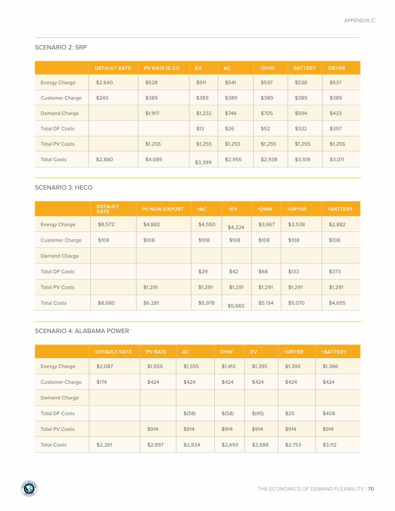
RO

C

KY MOUNTAIN

INSTIT UTE


APPENDIX C

SCENARIO 2: SRP

SCENARIO 3: HECO

DEFAULT RATE PV RATE (E-27) EV AC +DHW BATTERY DRYER

Energy Charge $2,640 $528 $511 $541 $537 $538 $537

Customer Charge $240 $389 $389 $389 $389 $389 $389

Demand Charge $1,917 $1,232 $746 $705 $594 $433

Total DF Costs $13 $26 $52 $332 $397

Total PV Costs $1,255 $1,255 $1,255 $1,255 $1,255 $1,255

Total Costs $2,880 $4,089 $3,399 $2,956 $2,938 $3,109 $3,011

DEFAULT RATE PV NON-EXPORT +AC +EV +DHW +DRYER +BATTERY

Energy Charge $8,572 $4,882 $4,550 $4,224 $3,667 $3,538 $2,882

Customer Charge $108 $108 $108 $108 $108 $108 $108

Demand Charge

Total DF Costs $29 $42 $68 $133 $373

Total PV Costs $1,291 $1,291 $1,291 $1,291 $1,291 $1,291

Total Costs $8,680 $6,281 $5,978 $5,665 $5,134 $5,070 $4,655

SCENARIO 4: ALABAMA POWER

DEFAULT RATE PV RATE AC DHW EV +DRYER +BATTERY

Energy Charge $2,087 $1,559 $1,555 $1,413 $1,395 $1,395 $1,366

Customer Charge $174 $424 $424 $424 $424 $424 $424

Demand Charge

Total DF Costs $(58) $(58) $(45) $20 $408

Total PV Costs $914 $914 $914 $914 $914 $914

Total Costs $2,261 $2,897 $2,834 $2,693 $2,688 $2,753 $3,112

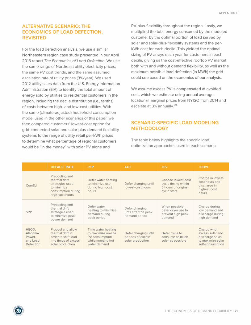
RO

C

KY MOUNTAIN

INSTIT UTE


APPENDIX C

ALTERNATIVE SCENARIO: THE ECONOMICS OF LOAD DEFECTION, REVISITED

For the load defection analysis, we use a similar Northeastern region case study presented in our April 2015 report The Economics of Load Defection. We use the same range of Northeast utility electricity prices, the same PV cost trends, and the same assumed escalation rate of utility prices (3%/year). We used 2012 utility sales data from the U.S. Energy Information Administration (EIA) to identify the total amount of energy sold by utilities to residential customers in the region, including the decile distribution (i.e., tenths) of costs between high- and low-cost utilities. With the same (climate-adjusted) household consumption model used in the other scenarios of this paper, we then compared customers’ lowest-cost option for grid-connected solar and solar-plus-demand flexibility systems to the range of utility retail per-kWh prices to determine what percentage of regional customers would be “in the money” with solar PV alone and

PV-plus-flexibility throughout the region. Lastly, we multiplied the total energy consumed by the modeled customer by the optimal portion of load served by solar and solar-plus-flexibility systems and the per-kWh cost for each decile. This yielded the optimal sizing of PV arrays each year for customers in each decile, giving us the cost-effective rooftop PV market both with and without demand flexibility, as well as the maximum possible load defection (in MWh) the grid could see based on the economics of our analysis.

We assume excess PV is compensated at avoided cost, which we estimate using annual average locational marginal prices from NYISO from 2014 and escalate at 3% annually.108

SCENARIO-SPECIFIC LOAD MODELING METHODOLOGY

The table below highlights the specific load optimization approaches used in each scenario.

DEFAULT RATE RTP +AC +EV +DHW

ComEd

Precooling and thermal drift strategies used to minimize consumption during high-cost hours

Defer water heating to minimize use during high-cost hours

Defer charging until lowest-cost hours

Choose lowest-cost cycle timing within 6 hours of original cycle start

Charge in lowest-cost hours and discharge in highest-cost hours

SRP

Precooling and thermal drift strategies used to minimize peak power demand

Defer water heating to minimize demand during peak period

Defer charging until after the peak demand period

When possible defer dryer use to prevent high peak demand

Charge during low demand and discharge during high demand

HECO, Alabama Power, and Load Defection

Precool and allow thermal drift in order to shift load into times of excess solar production

Time water heating to maximize on-site PV consumption while meeting hot water demand

Defer charging until periods of excess solar production

Defer cycle to consume as much solar as possible

Charge when excess solar and discharge so as to maximize solar self-consumption

APPENDIX D

SCENARIO MARKET SIZING

RO

C

KY MOUNTAIN

INSTIT UTE


APPENDIX DSCENARIO MARKET SIZING

To estimate the potential market for bill savings, solar installation, and controls investment that is unlocked by demand flexibility, we scale the results for our single, modeled customer premises to the potential market for other eligible utility customers served by the same utility.

PARTICIPATING CUSTOMER MARKET SIZING

For the ComEd scenario, there are roughly 10,000 customers already taking service under the analyzed RRTP rate. We scale our modeled results to these 10,000 customers after first scaling down the modeled savings and necessary investment to correspond to an average ComEd customer’s annual consumption, estimated using EIA Form 861 data from 2013.109

NON-PARTICIPATING CUSTOMER MARKET SIZING

For all four scenarios, we estimate the number of customers who could achieve cost savings using demand flexibility by switching from default, volumetric rates to the rates analyzed. We use EIA Form 861 data to assess the number of customers who may be eligible to switch. For ComEd, this is the sum of all ComEd customers as well as customers of competitive electric suppliers whose electricity is delivered by ComEd.

For the other three scenarios, customers are only able to switch to the rates analyzed and achieve savings with demand flexibility if they install a rooftop PV system. We assume that only owner-occupied, single-family homes that have sufficient roof space

to host PV panels are eligible to install PV. We use data from the U.S. Census on state-specific home ownership rates and the percentage of units that are multi-family,110 and use NREL estimates of the potential for U.S. residential buildings to host at least 1.5 kWdc of rooftop PV capacity (81%) and the average size of installed rooftop PV (4.9 kWdc).

111 We multiply EIA Form 861 records for the number of residential customers for each utility by these derating factors to arrive at an estimate of the number of potential PV-adopting customers in each jurisdiction.

To estimate the net bill savings potential, we scale our modeled customer’s savings to utility-specific average consumption levels for residential customers. To estimate the solar PV market enabled, we multiply the average PV array size from NREL by the number of eligible houses, and convert to dollars using the assumed installation price for residential PV of $3.50/Wdc. To estimate the vendor market, we scale the total capital cost of all cost-effective flexibility measures for our modeled customer in each scenario by the ratio of average to modeled customer consumption.

For scenarios 1 and 2, we also estimate the utility-wide peak demand reduction potential unlocked by residential DF. We estimate the percentage peak demand reduction realized using our model during either system coincident peak (ComEd) or on average across all peak periods each month (SRP), and multiply that peak reduction by residential customer average peak demand using data from the 2009 FERC National Assessment of Demand Response Potential.112

ENDNOTES

RO

C

KY MOUNTAIN

INSTIT UTE


ENDNOTES

ENDNOTES

1 A Review of Solar PV Benefit & Cost Studies, Rocky Mountain Institute, 2013, http://www.rmi.org/elab_empower.

2 Quadrennial Energy Review, U.S. Department of Energy, http://energy.gov/epsa/downloads/quadrennial-energy-review-full-report.

3 Peter Bronski, “The U.S. Electric Grid has a Baby Boomer Social Security Problem,” Rocky Mountain Institute, September 24, 2014, http://blog.rmi.org/blog_2014_09_24_us_electric_grid_has_a_baby_boomer_social_security_problem.

4 “Retail Sales of Electricity to Ultimate Customers,” U.S. Energy Information Administration, http://www.eia.gov/electricity/monthly/epm_table_grapher.cfm?t=epmt_5_01.

5 “Peak-to-average electricity demand ratio rising in New England and many other U.S. regions,“ U.S. Energy Information Administration, http://www.eia.gov/todayinenergy/detail.cfm?id=15051.

6 “Monthly generator capacity factor data now available by fuel and technology,” U.S. Energy Information Administration, http://www.eia.gov/todayinenergy/detail.cfm?id=14611.

7 “Peak-to-average electricity demand ratio rising in New England and many other U.S. regions,” U.S. Energy Information Administration.

8 “Average Retail Price of Electricity to Ultimate Customers,” http://www.eia.gov/electricity/monthly/epm_table_grapher.cfm?t=epmt_5_3; and “Energy Prices by Sector and Source,” U.S. Energy Information Administration, 2015, http://www.eia.gov/forecasts/aeo/pdf/tbla3.pdf.

9 Dave Lamont and John Gerhard, The Treatment of Energy Efficiency in Integrated Resource Plans: A Review of Six State Practices, RAP, January 2013, http://www.raponline.org/document/download/id/6368; and John Sterling, et al., Treatment of Solar Generation in Electric Utility Resource Planning, National Renewable Energy Laboratory, October 2013, http://www.nrel.gov/docs/fy14osti/60047.pdf.

10 The Economics of Load Defection, Rocky Mountain Institute, April 2015, http://www.rmi.org/electricity_load_defection.

11 Mike Munsell, “Ruling Against FERC Order Could Cost U.S. Demand Response Market,” Greentech Media, September 2014, http://www.greentechmedia.com/articles/read/Ruling-Against-FERC-Order-Could-Cost-US-Demand-Response-Market-4.4B-in-Rev.

12 Audrey Zibelman, Energy Gang podcast, September 2014, https://soundcloud.com/the-energy-gang/new-york-is-creating-the-most-innovative-grid-in-the-world.

13 Munsell, http://www.greentechmedia.com/articles/read/Ruling-Against-FERC-Order-Could-Cost-US-Demand-Response-Market-4.4B-in-Rev.

14 EIA Form 861, 2013.

15 David Becker, “Smart Meters and Dynamic Pricing Need Each Other,” Great Lakes Symposium on Smart Grid and the New Energy Economy, September 2014, http://www.elevateenergy.org/prod/httpdocs/wp/wp-content/uploads/GL-Symposium-Smart-Meters-Dynamic-Pricing.pdf.

16 ComEd, https://rrtp.comed.com/.

17 Ameren, https://www.ameren.com/illinois/electric-choice/residential-real-time-pricing.

18 Jeff St. John, “California’s Major Residential Rate Reform: A Mixed Bag for Solar Economics,” Greentech Media, 2015, http://www.greentechmedia.com/articles/read/californias-major-residentia-rate-reform-a-mixed-bag-for-solar-economics.

19 Ryan Hledik, “Rediscovering Residential Demand Charges,” The Electricity Journal, 2014.

20 SRP, http://www.srpnet.com/prices/priceprocess/customergenerated.aspx.

21 APS, https://www.aps.com/en/residential/accountservices/serviceplans/Pages/combined-advantage.aspx.

22 “Direct Testimony of Ahad Faruqui on Behalf of Westar Energy,” https://www.westarenergy.com/Portals/0/Resources/Documents/RateCasePDF/Direct_Testimony_of_Ahmad_Faruqui_on_behalf_of_Westar_Energy.pdf.

24 “In the Matter of Commission Consideration of Retail Renewable Distributed Generation and Net Metering,” XCEL Energy, 2014, http://www.xcelenergy.com/staticfiles/xe/Marketing/Files/CPUC%20July%2024%202014%20Panel%20Discussion%20Xcel%20Energy%20Responses.pdf.

25 “TEP to Propose Revised Net Metering Plan in Request for New 2017 Rates,” TEP press release, June 19, 2015, https://www.tep.com/news/newsroom/release/?idRec=420.

26 Herman K. Trabish, “As Solar Grows, Madison Utility Seeks Rate Structure Challenge, Utility Dive, July 2014, http://www.utilitydive.com/news/as-solar-grows-madison-utility-seeks-rate-structure-change/291281/.

27 Gavin Bade, “Wisc. Regulators Approve 75% Increase in We Energies Fixed Charges,” Utility Dive, November 2014, http://www.utilitydive.com/news/wisc-regulators-approve-75-increase-in-we-energies-fixed-charges/333409/.

28 Thomas Content, “Wisconsin Public Service Seeks a Second Raise in Fixed Charges,” Journal Sentinel, May 2015, http://www.jsonline.com/business/wisconsin-public-service-seeks-a-second-raise-in-fixed-charges-b99502577z1-304154051.html.

29 “Kansas City Power and Light Rate Design Proposal,” Synapse, http://www.synapse-energy.com/project/kansas-city-power-and-light-rate-design-proposal-15-018.

RO

C

KY MOUNTAIN

INSTIT UTE


ENDNOTES

30 Steve Kihm, “Economic Concerns About High Fixed Charge Pricing for Electric Service,” http://americaspowerplan.com/wp-content/uploads/2014/10/Economic-analysis-of-high-fixed-charges.pdf; and “Designing Distributed Generation Tariffs Well: Ensuring Fair Compensation in a Time of Transition,“ Regulatory Assistance Project, http://www.raponline.org/press-release/designing-distributed-generation-tariffs-well-ensuring-fair-compensation-in-a-time-of.

31 Hawaii Public Service Commission, Docket 2014-0192, Order 32737, Staff Report and Proposal, March 31, 2015, 33-35, CAISO 2012, http://www.caiso.com/Documents/

32 A Review of Solar PV Benefit & Cost Studies, Rocky Mountain Institute, 2013.

33 Jim Lazar, “Electric Utility Residential Customer Charges and Minimum Bills: Alternative Approaches for Recovering Basic Distribution Costs,” Regulatory Assistance Project, 2014.

34 Katherine Tweed, “How Much Did Nest Labs Save Utilities Last Summer?” Greentech Media, May 15, 2014, http://www.greentechmedia.com/articles/read/how-much-did-nest-labs-save-utilities-last-summer; and Jeff St. John, “Ohmconnect Debuts New Demand Response Model,” Greentech Media, September 29, 2014, http://www.greentechmedia.com/articles/read/Ohmconnects-Home-Energy-to-Grid-Connection-is-a-New-Demand-Response-Model.

35 Stephen Lacy, “SolarCity Teams Up With Nest, Adding to the List of Solar-Smart Home Partnerships,” Greentech Media, April 13, 2015, http://www.greentechmedia.com/articles/read/solarcity-teams-up-with-nest-adding-to-the-list-of-solar-smart-home-partner.

36 PSEG Utility 2.0 Long Range Plan, July 1, 2014, https://www.psegliny.com/files.cfm/2014-07-01_PSEG_LI_Utility_2_0_LongRangePlan.pdf.

37 Audrey Zibelman, “Recommendations of PSEG First Annual Long Range Plan,” April 15, 2015, http://www.dps.ny.gov/longisland/DPS_Recommendations_of_PSEG_first_annual_long_range_plan.pdf.

38 Public Service Commission session, December 11, 2014, http://documents.dps.ny.gov/public/Common/ViewDoc.aspx?DocRefId=%7B83594C1C-51E2-4A1A-9DBB-5F15BCA613A2%7D.

39 “Hawaiian Electric Companies’ Motion for Approval of NEM Program Modification and Establishment of Transitional Distributed Generation Program Tariff, Public Utilities Commission, January 20, 2015, http://dms.puc.hawaii.gov/dms/DocumentViewer?pid=A1001001A15A20B13419D27829.

40 2013 Integrated Resource Planning Report, Hawaiian Electric Company, 22-11, http://www.hawaiianelectric.com/vcmcontent/IntegratedResource/IRP/PDF/IRP-2013-Report-Chapter-22.pdf.

41 Earle Ifuku et al., “Hawaiian Electric Grid Interactive Water Heater (GIWH) Demonstration Status,” http://c.ymcdn.com/sites/www.peakload.org/resource/resmgr/2014FallArchive/Harshal.pdf.

42 ComEd, https://rrtp.comed.com/.

43 SRP, http://www.srpnet.com/prices/priceprocess/customergenerated.aspx.

44 Ruling on the RSWG Work Product, Public Utilities Commission, April 2014, http://puc.hawaii.gov/wp-content/uploads/2014/04/Order-No.-32053.pdf.

45 Alabama Power, http://www.alabamapower.com/residential/pricing-rates/pae.asp.

46 Nest, “Energy Savings from the Nest Learning Thermostat: Energy Bill Analysis Results,” February 2015. https://nest.com/downloads/press/documents/energy-savings-white-paper.pdf.

47 Tesla Motors, http://www.teslamotors.com/presskit.

48 Howard Ng, “The Evolution of Communications for Demand Response (Second Edition),” Comverge, 2015; and Omar Saadeh, Energy in the Connected Home 2015: Technology Evolution, Landscape and Distribution Strategies, GTM Research, March 2015, http://www.greentechmedia.com/research/report/energy-in-the-connected-home-2015.

49 Robert Walton, “HECO completes first phase of smart grid rollout,” Utility Dive, September 25, 2014, http://www.utilitydive.com/news/heco-completes-first-phase-of-smart-grid-roll-out/313681/.

50 Edison Foundation Institute for Electric Innovation [IEI], “Utility-scale smart meter deployments,” September 2014.

51 Edison Foundation IEI, “Utility-scale smart meter deployments.”

52 Tim Woolf et al., “A Framework for Evaluating the Cost-effectiveness of Demand Response,” http://emp.lbl.gov/sites/all/files/napdr-cost-effectiveness.pdf.

53 The Nest Store, https://store.nest.com/product/thermostat/ and Chevrolet, 2015 Chevy Volt User’s Manual, pp. 5-29, 5-30, http://www.chevrolet.com/content/dam/Chevrolet/northamerica/usa/nscwebsite/en/Home/Ownership/Manuals_and_Videos/02_pdf/2015-volt-owners-manual.pdf.

54 Amory Lovins and Rocky Mountain Institute, Reinventing Fire: Bold Business Solutions for the New Energy Era, October 2011, http://www.rmi.org/reinventingfire.

55 “A National Assessment of Demand Response Potential,” Federal Energy Regulatory Commission, June 2009, http://www.ferc.gov/legal/staff-reports/06-09-demand-response.pdf.

56 Ahmad Faruqui, et al., “The Power of Five Percent,” The Brattle Group, May 2007, sites.energetics.com/MADRI/pdfs/ArticleReport2441.pdf.

57 “A National Assessment of Demand Response Potential,” Federal Energy Regulatory Commission.

58 Johanna L. Mathieu et al., “Resource and revenue potential of California residential load participation in ancillary services,” Energy Policy, May 2015, http://www.sciencedirect.com/science/article/pii/S0301421515000427.

59 BESH Tariff, https://www.comed.com/documents/customer-service/rates-pricing/rates-information/current/05_ratebesh.pdf.

60 Nest, https://nest.com/support/article/About-the-Nest-energy-partners; and “ComEd Partners with Nest, Xfinity on Smart Thermostat Energy Saving Program,” The News, May 20, 2015, http://www.achrnews.com/articles/129653-may-20-2015-comed-partners-with-nest-xfinity-on-smart-thermostat-energy-saving-program.

61 Salt River Project E-27 Customer Generation Price Plan for Residential Service, http://www.srpnet.com/prices/pdfx/April2015/E-27.pdf.

62 Mark Jaffe, “Cost of solar power vexing to Colorado system owners, electric co-ops,” The Denver Post, June 7, 2015, http://www.denverpost.com/business/ci_28262200/cost-solar-power-vexing-colorado-system-owners-electric.

RO

C

KY MOUNTAIN

INSTIT UTE


ENDNOTES

63 Ibid.

64 Hawaii Public Service Commission, Docket 2011-0206, Order 32053, 46–47 and 54, http://dms.puc.hawaii.gov/dms/OpenDocServlet?RT=&document_id=91+3+ICM4+LSDB15+PC_DocketReport59+26+A1001001A14D29A91150C1040318+A14D29B10740F583001+14+1960.

65 Ibid.; and Hawaii Public Service Commission, Docket 2014-0192, Order 32737, Staff Report and Proposal, March 31, 2015. 33–35, http://dms.puc.hawaii.gov/dms/OpenDocServlet?RT=&document_id=91+3+ICM4+LSDB15+PC_DocketReport59+26+A1001001A15D01A84805H5843318+A15D01A92712J302731+14+1960.

66 Hawaiian Electric Companies’ Distributed Generation Interconnection Plan, August 2014, 5-10–5-12 http://files.hawaii.gov/puc/4_Book%201%20%28transmittal%20ltr_DGIP_Attachments%20A-1%20to%20A-5%29.pdf.

67 CAISO 2012, http://www.caiso.com/Documents/StrawProposal–FlexibleResourceAdequacyCriteriaMustOfferObligation.pdf

68 Alabama Power, http://www.alabamapower.com/residential/pricing-rates/pdf/fd.pdf.

69 Alabama Power, http://www.alabamapower.com/residential/pricing-rates/pdf/PAE.pdf.

70 Kyle Whitmire, “Let there be light,” AL.com, October 7, 2014. http://www.al.com/opinion/index.ssf/2014/10/let_there_me_light_how_solar_c.html.

77 The Economics of Load Defection, Rocky Mountain Institute, April 2015, http://www.rmi.org/electricity_load_defection.

78 Net Energy Metering: Subsidy Issues and Regulatory Solutions, Institute for Electric Innovation, September 2014, http://www.edisonfoundation.net/iei/documents/IEI_NEM_Subsidy_Issues_FINAL.pdf; and Arizona Corporation Commission Docket, http://images.edocket.azcc.gov/docketpdf/0000161533.pdf.

79 A Review of Solar PV Benefit & Cost Studies, Rocky Mountain Institute, 2013.

80 Rate Design for the Distribution Edge. Rocky Mountatin Institute. 2014. rmi.org/elab_rate_design.

81 Ibid.

82 The PowerShift Atlantic program offers maintenance for customers with controllable water heaters. Peter Stymiest, “GIWH Product Development,” 2013 ACEEE Hot Water Forum: http://aceee.org/files/pdf/conferences/hwf/2013/3C-stymiest.pdf.

83 Smart thermostats can monitor AC system performance and report issues. Rachel Reiss Buckley, “Capture smart thermostats for demand response while people care about them,” E Source E News, 30 April 2013.

84 Chris Mooney, “Want to get conservatives to save energy? Stop the environmentalist preaching,” The Washington Post, February 12, 2015, http://www.washingtonpost.com/news/energy-environment/wp/2015/02/12/the-best-way-to-get-conservatives-to-save-energy-is-to-stop-the-environmentalist-preaching/.

85 Andre Wellington, Interoperability of Demand Response Resources Demonstration in NY, ConEdison, February 2015, http://energy.gov/sites/prod/files/2015/03/f20/ConEd-RDSI_Interoperability-Project-Report-Feb2015.pdf.

86 Sunil Maulik, “Trends in Infrastructure: The Internet of Things,” Oracle, January 2014, http://www.oracle.com/us/corporate/profit/big-ideas/012314-smaulik-2112685.html; and The Internet of Things: Making sense of the next mega-trend, Goldman Sachs, September 2014, http://www.goldmansachs.com/our-thinking/outlook/internet-of-things/iot-report.pdf .

87 Ahmad Faruqui et al., “Smart By Default,” Public Utilities Fortnightly, August 2014, http://www.fortnightly.com/fortnightly/2014/08/smart-default.

71 PowerShift Atlantic, http://powershiftatlantic.com/faq.html.

72 NB Power, https://www.nbpower.com/en/products-services/water-heaters/.

73 David Podorson, Battery Killers: How Water Heaters Have Evolved into Grid-Scale Energy-Storage Devices, September 2014, http://www.esource.com/ES-WP-18/GIWHs.

74 Steele-Waseca Cooperative Electric, http://swce.com/documents/CommunitySolarFAQ.pdf.

75 SDG&E, http://www.sdge.com/regulatory-filing/10676/sdge-electric-vehicle-grid-integration-pilot-program.

76 Andrey Gunawan and Pourya Shamsi, “San Diego Electric Vehicles Growth,” IEEE Transportation Electrification, March 5, 2014, http://electricvehicle.ieee.org/2014/03/05/san-diego-electric-vehicles-growth/.

88 Ahmad Faruqui, The Power of Five Percent, The Brattle Group, May 2007, http://sites.energetics.com/madri/pdfs/ArticleReport2441.pdf.

89 NERC 2014 Long-Term Reliability Assessment (2015 Net Internal Demand).

90 2009 RECS Survey Data, U.S. Energy Information Administration, http://www.eia.gov/consumption/residential/data/2009/.

91 Data from Appendix D of National Assessment of Demand Response Potential, The Brattle Group, Freeman, Sullivan & Co, Global Energy Partners LLC, June 2009, http://www.ferc.gov/legal/staff-reports/06-09-demand-response.pdf.

92 Johanna L. Mathieu, Mark E.H. Dyson, and Duncan S. Callawy, “Resource and revenue potential of California residential load participation in ancillary services,” Energy Policy, May 2015, http://www.sciencedirect.com/science/article/pii/S0301421515000427; and Grayson Heffner et al., 2007, Loads providing ancillary services: review of international experience, Ernest Orlando Lawrence Berkeley National Laboratory, May 2007, http://www.energy.gov/sites/prod/files/oeprod/DocumentsandMedia/Loads_providing_Ancillary_Services_main_report_62701.pdf.

93 Jason MacDonald et al., “Demand Response Providing Ancillary Services A Comparison of Opoprtuntites and Challenges in the US Wholesale Markets,” 2012, http://eetd.lbl.gov/publications/dr-providing-as-comparison-opportunities-challenges.

94 NREL’s System Advisor Model, https://sam.nrel.gov/, accessed June 4, 2015.

95 Mike Munsell, “Solar PV Pricing Continues to Fall During a Record-Breaking 2014,“ Greentech Media, March 2015, http://www.greentechmedia.com/articles/read/solar-pv-system-prices-continue-to-fall-during-a-record-breaking-2014.

96 NREL Typical Meteorological Year (TMY3) Data, http://rredc.nrel.gov/solar/old_data/nsrdb/1991-2005/tmy3/by_state_and_city.html, accessed June 4, 2015.

RO

C

KY MOUNTAIN

INSTIT UTE


ENDNOTES

97 Northwest Energy Efficiency Alliance submetered energy data, http://neea.org/resource-center/regional-data-resources/residential-building-stock-assessment, accessed June 4, 2015.

98 Mathieu et al., “Resource and revenue potential of California residential load participation in ancillary services.”

99 Ron Judkoff et al., 2010 (NREL/TP-550-47427) in EnergyPlus v. 8.1.

100 Nest’s Energy Savings White Paper, June 2015, https://nest.com/downloads/press/documents/energy-savings-white-paper.pdf.

101 Energy Star Furnace Calculator, http://www.energystar.gov/buildings/sites/default/uploads/files/Furnace_Calculator.xls, accessed June 4, 2015.

102 EIA average delivered natural gas price, http://www.eia.gov/dnav/ng/ng_pri_sum_a_EPG0_PRS_DMcf_a.htm, accessed June 4, 2015.

103 The Nest Store, https://store.nest.com/product/thermostat/?utm_campaign=product-listing-ad&utm_source=google&utm_medium=cpc&utm_content=T200577&gclid=CPKbz93W0MUCFZWCaQoddbYAuw, accessed May 20, 2015 and Home Depot, http://www.homedepot.com/p/Honeywell-5-2-Day-Programmable-Thermostat-with-Backlight-RTH2300B/203539496?N=5yc1vZc4lf, accessed May 20, 2015.

104 Smart washer/dryer, http://www.homedepot.com/p/Whirlpool-Smart-4-3-cu-ft-High-Efficiency-Front-Load-Washer-in-Silver-ENERGY-STAR-WFL98HEBU/205037982, accessed May 20, 2015 and baseline washer/dryer, http://www.homedepot.com/p/Whirlpool-Duet-4-3-cu-ft-High-Efficiency-Front-Load-Washer-with-Steam-in-Chrome-Shadow-ENERGY-STAR-WFW87HEDC/205361272, accessed May 20, 2015.

105 James Manyika et al., 2015, “Unlocking the potential of the Internet of Things,” McKinsey & Company: http://www.mckinsey.com/insights/business_technology/The_Internet_of_Things_The_value_of_digitizing_the_physical_world.

106 COMED FAQ, https://rrtp.comed.com/faqs/, accessed June 4, 2015.

107 PJM Historical Load Data, http://www.pjm.com/markets-and-operations/ops-analysis/historical-load-data.aspx, accessed June 4, 2015.

108 NYISO, http://www.nyiso.com/public/markets_operations/market_data/pricing_data/index.jsp, as compiled at http://www.energyonline.com/Data/GenericData.aspx?DataId=12&NYISO___Actual_Energy_Price, accessed June 4, 2015.

109 Electric power sales, revenue, and energy efficiency Form EIA-861, U.S. Energy Information Administration, http://www.eia.gov/electricity/data/eia861/.

110 United States Census, http://quickfacts.census.gov/qfd/states/.

111 David Feldman, Anna M. Brockway, Elaine Ulrich, and Robert Margolis, Shared Solar: Current Landscape, Market Potential, and the Impact of Federal Securities Regulation, National Renewable Energy Laboratory, April 2015, www.nrel.gov/docs/fy15osti/63892.pdf.

112 A National Assessment of Demand Response Potential, FERC 2009, http://www.ferc.gov/legal/staff-reports/06-09-demand-response.pdf (Table D-6).