the effect of social connectedness on crime: evidence from...
TRANSCRIPT
The Effect of Social Connectedness on Crime:Evidence from the Great Migration∗
Bryan A. StuartGeorge Washington University
Evan J. TaylorUniversity of Chicago
August 23, 2017
Abstract
This paper estimates the effect of social connectedness on crime across U.S. cities from 1960-2009. Migration networks among African Americans from the South generated variationacross destinations in the concentration of migrants from the same birth town. Using this novelsource of variation, we find that social connectedness considerably reduces murders, robberies,assaults, burglaries, larcenies, and motor vehicle thefts, with a one standard deviation increasein social connectedness reducing murders by 13 percent and motor vehicle thefts by 9 percent.Our results appear to be driven by stronger relationships among older generations reducingcrime committed by youth.
JEL Classification Codes: K42, N32, R23, Z13
Keywords: crime, social connectedness, Great Migration
∗Thanks to Martha Bailey, Dan Black, John Bound, Charlie Brown, John DiNardo, Alan Griffith, Mike Muller-Smith, Daniel Nagin, Seth Sanders, Jeff Smith, Lowell Taylor, Anthony Yezer, and numerous seminar and confer-ence participants for helpful comments. Thanks to Seth Sanders and Jim Vaupel for facilitating access to the DukeSSA/Medicare data. During work on this project, Stuart was supported in part by an NICHD training grant (T32HD007339) and an NICHD center grant (R24 HD041028) to the Population Studies Center at the University of Michi-gan.

1 Introduction
For almost 200 years, the enormous variance of crime rates across space has intrigued social scien-
tists and policy makers (Guerry, 1833; Quetelet, 1835; Weisburd, Bruinsma and Bernasco, 2009).
Standard covariates explain relatively little of the cross-city variation in crime, which suggests a
potential role for social influences (Glaeser, Sacerdote and Scheinkman, 1996). One possible ex-
planation is peer effects, whereby an individual is more likely to commit crime if his peers commit
crime (e.g., Case and Katz, 1991; Glaeser, Sacerdote and Scheinkman, 1996; Damm and Dust-
mann, 2014). A non-rival explanation is that cities differ in the degree of social connectedness, or
the strength of relationships between individuals, including those unlikely to commit crime.
There is widespread interest in the effects of social connectedness and the related concept of
social capital. This interest partly stems from the possibility that relationships between individuals
can address market failures and generate desirable outcomes that are difficult to accomplish with
government policies. However, estimating the effects of social connectedness and social capital
has proven challenging. Some of the most influential evidence comes from correlations between
outcomes, such as income and crime, and proxies for social capital, like individuals’ participation
in community organizations, their stated willingness to intervene in the community, and their stated
willingness to trust others (Sampson, Raudenbush and Earls, 1997; Putnam, 2000). These proxies
for social capital reflect individuals’ contemporaneous decision to invest in their community, which
raises the concern that these correlations reflect reverse causality or omitted variables bias. As a
result, the empirical importance of social capital continues to be debated (Durlauf, 2002).
This paper uses a new source of variation in social connectedness to estimate its effect on crime.
Migration networks among millions of African Americans who moved out of the U.S. South from
1915-1970 generated variation across destinations in the concentration of migrants from the same
birth town. For example, consider Beloit, Wisconsin and Middletown, Ohio, two cities similar
along many dimensions, including the total number of Southern black migrants that moved there.
Around 18 percent of Beloit’s black migrants came from Pontotoc, Mississippi, while less than
five percent of Middletown’s migrants came from any single town. Historical accounts trace the
1
sizable migration from Pontotoc to Beloit to a single influential migrant getting a job in 1914 at
a manufacturer in search of workers. Furthermore, ethnographic and newspaper accounts suggest
that Southern birth town networks translated into strong community ties in the North. Guided by a
simple economic model, we proxy for social connectedness using a Herfindahl-Hirschman Index
of birth town to destination city population flows for African Americans born in the South from
1916-1936, who we observe in the Duke SSA/Medicare dataset.
We estimate regressions that relate cross-city differences in crime from 1960-2009 to cross-city
differences in social connectedness. Our main specification controls for the number of Southern
black migrants that live in each city, to adjust for differences in the overall attractiveness of cities
to black migrants, plus a rich set of demographic and economic variables and state-by-year fixed
effects, to adjust for many potential determinants of crime. City-level crime counts come from
FBI Uniform Crime Reports, which are widely available starting in 1960. We focus on social
connectedness among black migrants because birth town migration networks are especially strong
among this group (Stuart and Taylor, 2017) and qualitative and quantitative evidence supports our
resulting empirical strategy.
We find that social connectedness leads to sizable reductions in crime rates. At the mean,
a one standard deviation increase in social connectedness leads to a precisely estimated 13 per-
cent decrease in murder, the best measured crime in FBI data. Our estimates imply that replacing
Middletown’s social connectedness with that of Beloit would decrease murders by 23 percent, rob-
beries by 26 percent, and motor vehicle thefts by 16 percent. By comparison, the estimates in
Chalfin and McCrary (2015) imply that a similar decrease in murders would require a 34 percent
increase in the number of police officers. The elasticity of crime with respect to social connect-
edness ranges from -0.05 to -0.19 across the seven index crimes of murder, rape, robbery, assault,
burglary, larceny, and motor vehicle theft, and is statistically distinguishable from zero for every
crime besides rape.
A number of additional results clarify our main finding. Social connectedness reduces crimes
that are more and less likely to have witnesses, which suggests that an increased probability of
2

detection is not the only operative mechanism. The effect of social connectedness on crime does
not appear to be driven by effects on employment, education, homeownership, the prevalence
of single parents, or crack cocaine use. Other mechanisms, such as effects on norms, values,
or skills, likely matter. Social connectedness especially reduces crimes committed by African
American youth, who belong to the generations of migrants’ children, grandchildren, and great-
grandchildren. We also find that social connectedness reduces crimes committed by non-black
individuals, consistent with cross-race peer effects or spillovers. The estimated effects decline
over time, in line with the decline in the effective strength of our measure of social connectedness,
as Southern black migrants aged and eventually died.
Several pieces of evidence support the validity of our empirical strategy. Historical accounts
point to the importance of migrants who were well connected in their birth town and who worked
for an employer in search of labor in establishing concentrated migration flows from Southern
birth towns to Northern cities (Scott, 1920; Bell, 1933; Gottlieb, 1987; Grossman, 1989). Pioneer
migrants, making initial location decisions in the 1910s, established the migration patterns that
underlie subsequent variation in social connectedness. Consistent with a dominant role for such
idiosyncratic factors, social connectedness is not correlated with crime rates from 1911-1916. We
show that our results cannot be explained by migrants from the same birth town tending to move
to cities with low unobserved determinants of crime and these unobserved factors persisting over
time. Our results also are robust to controlling for the share of migrants in each destination that
moved there because of their birth town migration network, a variable we estimate from a novel
structural model of location decisions. Consequently, our estimates reflect the effect of social
connectedness per se, as opposed to unobserved characteristics of certain migrants.
This paper contributes most directly to the literature studying how characteristics of social net-
works affect crime (Sampson, Raudenbush and Earls, 1997; Putnam, 2000). We also contribute
to the literature in economics studying the impact of social capital and trust on various outcomes,
including growth and development (Knack and Keefer, 1997; Miguel, Gertler and Levine, 2005),
government efficiency and public good provision (La Porta et al., 1997; Alesina, Baqir and East-
3
erly, 1999, 2000), financial development (Guiso, Sapienza and Zingales, 2004), and microfinance
(Karlan, 2005, 2007; Cassar, Crowley and Wydick, 2007; Feigenberg, Field and Pande, 2013).
Our primary contribution is new, more credible evidence on the effect of social connectedness on
crime. We use variation in social connectedness that has the unusual and attractive property of be-
ing established decades before we measure outcomes as the result of a known process (birth town
migration networks).1 We also develop and parametrize a simple economic model that quantifies
the potentially important role of peer effects in amplifying the effects of social connectedness on
crime.
More broadly, there is enormous interest in the causes and consequences of criminal activity
and incarceration in U.S. cities, especially for African Americans (Freeman, 1999; Neal and Rick,
2014; Evans, Garthwaite and Moore, 2016), and this paper demonstrates the importance of social
connectedness in reducing crime. We also add to the literature on the consequences of the Great
Migration for migrants and cities, which has not considered the effects of social connectedness
before (e.g., Scroggs, 1917; Smith and Welch, 1989; Carrington, Detragiache and Vishwanath,
1996; Collins, 1997; Boustan, 2009, 2010; Hornbeck and Naidu, 2014; Black et al., 2015). This
paper draws on Stuart and Taylor (2017), which examines the role of birth town migration networks
among African Americans in more detail.
2 Historical Background on the Great Migration
The Great Migration saw nearly six million African Americans leave the South from 1910 to
1970 (Census, 1979).2 Although migration was concentrated in certain destinations, like Chicago,
Detroit, and New York, other cities also experienced dramatic changes. For example, Chicago’s
1Social connectedness is a broader concept than social capital, trust, or collective efficacy. For example, socialconnectedness might reduce crime by increasing the probability that criminals are identified, and this behavior typicallyis not included in definitions of social capital, trust, or collective efficacy. At the same time, our measure might capturesocial capital that was transported from the South. Definitions of social capital vary, but Portes (1998) argues that aconsensus definition is “the ability of actors to secure benefits by virtue of membership in social networks or othersocial structures” (p. 6). Fukuyama (1995), Putnam (2000), and Bowles and Gintis (2002) emphasize the role of trustand reciprocity in their definition of social capital. Karlan (2007) makes a similar distinction between social capitaland social connections as we do.
2Parts of this section come from Stuart and Taylor (2017).
4

black population share increased from two to 32 percent from 1910-1970, while Racine, Wisconsin
experienced an increase from 0.3 to 10.5 percent (Gibson and Jung, 2005). Migration out of the
South increased from 1910-1930, slowed during the Great Depression, and then resumed forcefully
from 1940 to the 1970s.
Several factors contributed to the exodus of African Americans from the South. World War
I, which simultaneously increased labor demand among Northern manufacturers and decreased
labor supply from European immigrants, helped spark the Great Migration, although many un-
derlying causes existed long before the war (Scroggs, 1917; Scott, 1920; Gottlieb, 1987; Marks,
1989; Jackson, 1991; Collins, 1997; Gregory, 2005). Underlying causes included a less developed
Southern economy, the decline in agricultural labor demand due to the boll weevil’s destruction
of crops (Scott, 1920; Marks, 1989, 1991; Lange, Olmstead and Rhode, 2009), widespread labor
market discrimination (Marks, 1991), and racial violence and unequal treatment under Jim Crow
laws (Tolnay and Beck, 1991).
Migrants tended to follow paths established by railroad lines: Mississippi-born migrants pre-
dominantly moved to Illinois and other Midwestern states, and South Carolina-born migrants
predominantly moved to New York and Pennsylvania (Scott, 1920; Carrington, Detragiache and
Vishwanath, 1996; Collins, 1997; Boustan, 2010; Black et al., 2015). Labor agents, offering paid
transportation, employment, and housing, directed some of the earliest migrants, but their role di-
minished sharply after the 1920s, and most individuals paid for the relatively expensive train fares
themselves (Gottlieb, 1987; Grossman, 1989).3 African-American newspapers from the largest
destinations circulated throughout the South, providing information on life in the North (Gottlieb,
1987; Grossman, 1989).4
Historical accounts and recent quantitative work indicate that birth town migration networks
strongly affected location decisions during the Great Migration. Initial migrants, most of whom
moved in the 1910s, chose their destination primarily in response to economic opportunity. Mi-
3In 1918, train fare from New Orleans to Chicago cost $22 per person, when Southern farmers’ daily wagestypically were less than $1 and wages at Southern factories were less than $2.50 (Henri, 1975).
4The Chicago Defender, perhaps the most prominent African-American newspaper of the time, was read in 1,542Southern towns and cities in 1919 (Grossman, 1989).
5

grants who worked for an employer in search of labor and were well connected in their birth town
linked friends, family, and acquaintances to jobs and shelter in the North, sometimes leading to
persistent migration flows from birth town to destination city (Rubin, 1960; Gottlieb, 1987). De-
scribing this behavior shortly after the start of the Great Migration, Scott (1920) wrote,
“The tendency was to continue along the first definite path. Each member of the
vanguard controlled a small group of friends at home, if only the members of his
immediate family. Letters sent back, representing that section of the North and giv-
ing directions concerning the route best known, easily influenced the next groups to
join their friends rather than explore new fields. In fact, it is evident throughout the
movement that the most congested points in the North when the migration reached its
height, were those favorite cities to which the first group had gone” (p. 69).
In Stuart and Taylor (2017), we show that birth town migration networks strongly influenced the
location decisions of African American migrants from the South.
The experience of John McCord captures many important features of early black migrants’
location decisions.5 Born in Pontotoc, Mississippi, nineteen-year-old McCord traveled in search
of higher wages in 1912 to Savannah, Illinois, where a fellow Pontotoc-native connected him with
a job. McCord moved to Beloit, Wisconsin in 1914 after hearing of employment opportunities and
quickly began work as a janitor at the manufacturer Fairbanks Morse and Company. After two
years in Beloit, McCord spoke to his manager about returning home for a vacation. The manager
asked McCord to recruit workers during the trip, and McCord returned with 18 unmarried men,
all of whom were soon hired. Thus began a persistent flow of African Americans from Pontotoc
to Beloit: among individuals born from 1916-1936, 14 percent of migrants from Pontotoc lived in
Beloit’s county in old age (Stuart and Taylor, 2017).6
Qualitative evidence documents the impact of social ties among African Americans from the
same birth town on life in the North. For example, roughly 1,000 of Erie, Pennsylvania’s 11,600
5The following paragraph draws on Bell (1933). See also Knowles (2010).6This is 68 times larger than the percent of migrants from Mississippi that lived in Beloit’s county at old age.
6

African American residents once lived in Laurel, Alabama, and almost half had family connections
to Laurel, leading an Erie resident to say, “I’m surrounded by so many Laurelites here, it’s like a
second home” (Associated Press, 1983). Nearly forty percent of the migrants in Decatur, Illinois
came from Brownsville, Tennessee, and Brownsville high school reunions took place in Decatur
from the 1980s to 2000s (Laury, 1986; Smith, 2006).7 As described by a Brownsville native,
“Decatur’s a little Brownsville, really” (Laury, 1986). Ethnographic work by Stack (1970) details
the importance of birth town and family social ties among African Americans for childrearing and
other behaviors. Motivated by these accounts, we now turn to a systematic analysis of the effect of
social connectedness on crime.
3 A Simple Model of Crime and Social Connectedness
Social connectedness could reduce crime through multiple channels, such as promoting stronger
norms, values, and skills or increasing the probability that criminals are identified and punished.
In this section, we use a simple economic model to derive an empirical measure of social con-
nectedness, and we show how the overall effect of social connectedness on crime depends on peer
effects.
3.1 Individual Crime Rates
We focus on a single city and characterize individuals by their age and social ties. For simplicity,
we consider a static model in which each younger individual makes a single decision about whether
to commit crime, while older individuals do not commit crime. Each individual belongs to one of
three groups: African Americans with ties to the South (τ = s), African Americans without ties
to the South (τ = n), and all others (τ = w). Older individuals have a tie to the South if they
were born there. Younger individuals have a tie to the South if at least one parent, who is an older
individual, was born in the South. We index younger individuals by i and older individuals by o.
7The 40 percent figure comes from the Duke SSA/Medicare dataset, described below.
7

For a younger individual who is black with ties to the South, we model the probability of
committing crime as
E[Ci|τi = s, ji = j] = αs + βs E[C−i] +∑o
γsi,o,j, (1)
where Ci = 1 if person i commits crime and Ci = 0 otherwise, and ji denotes the birth town
of i’s parents. Equation (1) is a linear approximation to the optimal crime rule from a utility-
maximizing model in which the relative payoff of committing crime depends on three factors. First,
αs, which is common to all individuals of type s, captures all non-social determinants of crime
(e.g., due to the number of police or employment opportunities). Second, an individual’s decision
to commit crime depends on the expected crime rate among peers, E[C−i]. Finally, the effect of
social connectedness is∑
o γsi,o,j , where γsi,o,j is the influence of older individual o on younger
individual i. This reduced-form representation captures several possible channels through which
social connectedness might affect crime. For example, older individuals might reduce crime among
younger individuals by increasing younger individuals’ stock of cognitive and non-cognitive skills,
which boost earnings in the non-crime labor market (Heckman, Stixrud and Urzua, 2006), by
promoting anti-crime norms and values (Stack, 1970), or by increasing the probability a criminal
is identified and punished (Becker, 1968). Alternatively, social connectedness could increase crime
by reinforcing unproductive norms or providing trust that facilitates criminal activity, as with the
Ku Klux Klan, Mafia, or gangs (Fukuyama, 2000; Putnam, 2000). Ultimately, whether social
connectedness decreases or increases crime is an empirical question.
Motivated by the qualitative evidence described in Section 2, we model social connectedness as
a function of whether the parents of individual i share a birth town with individual o. In particular,
γsi,o,j = γsH if the individuals share a birth town connection, ji = jo, and γsi,o,j = γsL otherwise. We
assume that younger African Americans with ties to the South are only influenced by older African
Americans with ties to the South, so that γsi,o,j = 0 if τi 6= τo. Given these assumptions, the effect
of social connectedness on person i is a weighted average of the high connectedness effect (γsH)
8
and the low connectedness effect (γsL),
∑o
γsi,o,j =N sj,0
N s0
γsH +
(1−
N sj,0
N s0
)γsL, (2)
where N sj,0 is the number of older individuals of type s from birth town j, and N s
0 =∑
j Nsj,0 is
the total number of older individuals in the city. Because social interactions depend on birth town
connections, the older generation’s migration decisions lead to differences in expected crime rates
for younger individuals with ties to different birth towns.
The Herfindahl-Hirschman Index emerges as a natural way to measure social connectedness in
this model. In particular, the probability that a randomly chosen African American with ties to the
South commits crime is
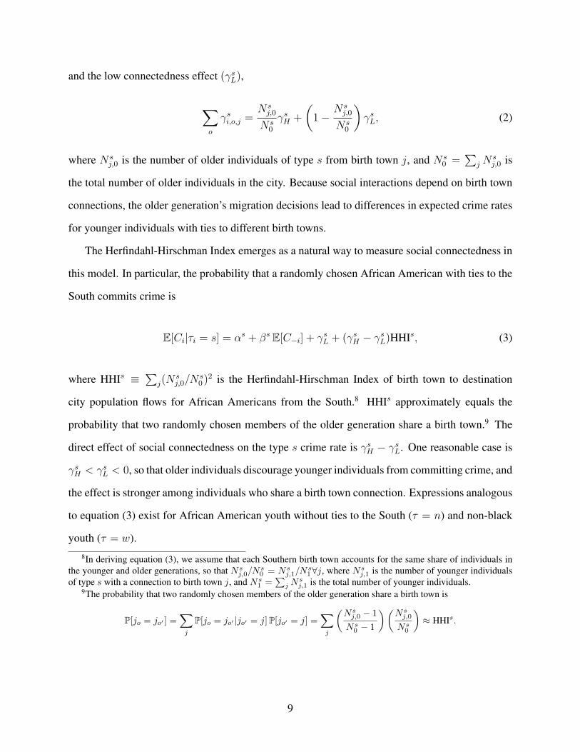
E[Ci|τi = s] = αs + βs E[C−i] + γsL + (γsH − γsL)HHIs, (3)
where HHIs ≡∑
j(Nsj,0/N
s0 )2 is the Herfindahl-Hirschman Index of birth town to destination
city population flows for African Americans from the South.8 HHIs approximately equals the
probability that two randomly chosen members of the older generation share a birth town.9 The
direct effect of social connectedness on the type s crime rate is γsH − γsL. One reasonable case is
γsH < γsL < 0, so that older individuals discourage younger individuals from committing crime, and
the effect is stronger among individuals who share a birth town connection. Expressions analogous
to equation (3) exist for African American youth without ties to the South (τ = n) and non-black
youth (τ = w).
8In deriving equation (3), we assume that each Southern birth town accounts for the same share of individuals inthe younger and older generations, so that Ns
j,0/Ns0 = Ns
j,1/Ns1∀j, where Ns
j,1 is the number of younger individualsof type s with a connection to birth town j, and Ns
1 =∑j N
sj,1 is the total number of younger individuals.
9The probability that two randomly chosen members of the older generation share a birth town is
P[jo = jo′ ] =∑j
P[jo = jo′ |jo′ = j]P[jo′ = j] =∑j
(Nsj,0 − 1
Ns0 − 1
)(Nsj,0
Ns0
)≈ HHIs.
9

3.2 City-Level Crime Rates
In the equilibrium of this model, peer effects can magnify or diminish the effect of social connect-
edness on crime. We use HHI to measure social connectedness and allow peer effects to differ by
the type of peer, leading to the following equilibrium,
Cs = F s(αs,HHIs, Cs, Cn, Cw) (4)
Cn = F n(αn,HHIn, Cs, Cn, Cw) (5)
Cw = Fw(αw,HHIw, Cs, Cn, Cw), (6)
where Cτ is the crime rate among younger individuals of type τ , and F τ characterizes the equi-
librium crime rate responses. The equilibrium crime rate vector (Cs, Cn, Cw) is a fixed point of
equations (4)-(6).
We are interested in the effect of social connectedness among African Americans with ties to
the South, HHIs, on equilibrium crime rates. Equations (4)-(6) imply that
dCs
dHHIs=
∂F s
∂HHIs
((1− J22)(1− J33)− J23J32
det(I − J)
)≡ ∂F s
∂HHIsms (7)
dCn
dHHIs=
∂F s
∂HHIs
(J23J31 + J21(1− J33)
det(I − J)
)≡ ∂F s
∂HHIsmn (8)
dCw
dHHIs=
∂F s
∂HHIs
(J21J32 + J31(1− J22)
det(I − J)
)≡ ∂F s
∂HHIsmw, (9)
where I is the 3 × 3 identity matrix and J , a sub-matrix of the Jacobian of equations (4)-(6),
captures the role of peer effects.10 Equations (7)-(9) depend on the direct effect of HHIs on crime
among African Americans with ties to the South, ∂F s/∂HHIs, and peer effect multipliers, ms,mn,
and mw. We assume the equilibrium is stable, which essentially means that peer effects are not too
10In particular,
J ≡
∂F s/∂Cs ∂F s/∂Cn ∂F s/∂Cw
∂Fn/∂Cs ∂Fn/∂Cn ∂Fn/∂Cw
∂Fw/∂Cs ∂Fw/∂Cn ∂Fw/∂Cw
,and Jab is the (a, b) element of J . ms is the (1, 1) element of (I − J)−1, mn is the (2, 1) element, and mw is the(3, 1) element.
10
large.11 For example, if J11 ≡ ∂F s/∂Cs ≥ 1, and there are no cross-group peer effects, then a
small increase in the crime rate among type s individuals leads to an equilibrium where all type s
individuals commit crime. In a stable equilibrium, a small change in any group’s crime rate does
not lead to a corner solution.
Our main theoretical result is that if social connectedness reduces the crime rate of African
Americans with ties to the South, then social connectedness reduces the crime rate of all groups,
as long as the equilibrium is stable and peer effects (i.e., elements of J) are non-negative.
Proposition 1. dCs/dHHIs ≤ 0, dCn/dHHIs ≤ 0, and dCw/dHHIs ≤ 0 if ∂F s/∂HHIs < 0, the
equilibrium is stable, and peer effects are non-negative.
In a stable equilibrium with non-negative peer effects, the crime-reducing effect of social con-
nectedness among Southern African Americans is not counteracted by higher crime rates among
other groups. Hence, equilibrium crime rates of all groups weakly decrease in Southern black
social connectedness. With negative cross-group peer effects, the reduction in crime rates among
Southern African Americans could lead to higher crime by other groups. A symmetric result holds
if social connectedness instead increases the crime rate of African Americans with ties to the South.
Proposition 1 is not surprising, and we provide a proof in Appendix A.
Because of data limitations, most of our empirical analysis examines the city-level crime rate,
C, which is a weighted average of the three group-specific crime rates,
C = P b[P s|bCs + (1− P s|b)Cn] + (1− P b)Cw, (10)
where P b is the black population share and P s|b is the share of the black population with ties to
the South. Proposition 1 provides sufficient, but not necessary, conditions to ensure that Southern
black social connectedness decreases the city-level crime rate, C, when the direct effect is negative.
There exist situations in which cross-group peer effects are negative, but an increase in HHIs
11The technical assumption underlying stability is that the spectral radius of J is less than one. This condition isanalogous to the requirement in linear-in-means models that the slope coefficient on the endogenous peer effect is lessthan one in absolute value (e.g., Manski, 1993).
11
still decreases the city-level crime rate. Guided by this theoretical analysis, we next describe our
empirical strategy for estimating the effect of social connectedness on crime.
4 Data and Empirical Strategy
4.1 Data on Crime, Social Connectedness, and Control Variables
To estimate the effect of social connectedness on crime, we use three different data sets. We mea-
sure annual city-level crime counts using FBI Uniform Crime Report (UCR) data for 1960-2009,
available from ICPSR. UCR data contain voluntary monthly reports on the number of offenses
reported to police, which we aggregate to the city-year level.12 We focus on the seven commonly
studied index crimes: murder and non-negligent manslaughter (“murder”), forcible rape (“rape”),
robbery, assault, burglary, larceny, and motor vehicle theft. Murder is the best measured crime,
and robbery and motor vehicle theft are also relatively well-measured (Blumstein, 2000; Tibbetts,
2012). Missing crimes are indistinguishable from true zeros in the UCR. Because cities in our
sample almost certainly experience property crime each year, we drop all city-years in which any
of the three property crimes (burglary, larceny, and motor vehicle theft) equal zero.13 We also use
annual population estimates from the Census Bureau in the UCR data.
The Duke SSA/Medicare dataset provides the birth town to destination city population flows
that underlie our measure of social connectedness. The data contain sex, race, date of birth, date of
death (if deceased), and the ZIP code of residence at old age (death or 2001, whichever is earlier)
for over 70 million individuals who received Medicare Part B from 1976-2001. In addition, the data
include a 12-character string with self-reported birth town information from the Social Security
Administration NUMIDENT file, which is matched to places, as described in Black et al. (2015).
These data capture long-run location decisions, as we only observe individuals’ location at birth
12We use Federal Information Processing System (FIPS) place definitions of cities. We follow Chalfin and McCrary(2015) in decreasing the number of murders for year 2001 in New York City by 2,753, the number of victims of theSeptember 11 terrorist attack.
13Out of 21,183 city-years in the data, at least one of the three property crimes equals zero for 956 city-years (4.5percent).
12

and old age.14 As a result, our measure of social connectedness for each city does not vary over
time. We focus on individuals born from 1916-1936 in the former Confederate states, which we
refer to as the South. Out-migration rates for the 1916-1936 cohorts are among the highest of all
cohorts in the Great Migration (Appendix Figure A.1), and coverage rates in the Duke data decline
considerably for earlier and later cohorts (Black et al., 2015). We restrict our main analysis sample
to cities with at least 25 Southern-born African American migrants in the Duke dataset to improve
the reliability of our estimates.
Census city data books provide numerous covariates for 1960, 1970, 1980, 1990, and 2000.
These data are only available for cities with at least 25,000 residents in 1960, 1980, and 1990, and
we apply the same restriction for 1970 and 2000. We limit our sample to cities in the Northeast,
Midwest, and West Census regions to focus on the cross-region moves that characterize the Great
Migration. Our main analysis sample excludes cities with especially severe measurement errors
in the crime data, as described in Appendix B. Appendix Tables A.1 and A.2 provide summary
statistics.
4.2 Estimating the Effect of Social Connectedness on Crime
Our main estimating equation is
Yk,t = exp[ln(HHIk)δ + ln(Nk)θ +X ′k,tβ] + εk,t, (11)
where Yk,t is the number of crimes in city k in year t. The key variable of interest is our proxy for
social connectedness among African Americans with ties to the South, HHIk =∑
j (Nj,k/Nk)2,
where Nj,k is the number of migrants from birth town j that live in destination city k, and Nk ≡∑j Nj,k is the total number of migrants. A Herfindahl-Hirschman Index is a natural way to mea-
sure social connectedness, as shown in Section 3. Xk,t is a vector of covariates, including log pop-
14As described in detail below, there was relatively little migration for our sample after leaving the South, so ourability to observe individuals’ location only in old age is not particularly important.
13

ulation and other variables described below, and εk,t captures unobserved determinants of crime.15
We use an exponential function in equation (11) because there are no murders for many city-year
observations (Appendix Table A.1).16
Our proxy for social connectedness varies only across cities, but the number of crimes varies
across both cities and years. Instead of collapsing the data into city-level observations, we use
equation (11) to more flexibly control for the covariates in Xk,t and because our panel of cities
is not balanced. We cluster standard errors by city to allow for arbitrary autocorrelation in the
unobserved determinants of crime. As a result, the number of cities is most relevant for thinking
about the number of observations in our regressions.
The key parameter of interest is δ, which we interpret as the elasticity of the crime rate with
respect to HHIk, because we control for log population and specify the conditional mean as an
exponential function. If social connectedness reduces the city-level crime rate, then δ < 0. We
estimate δ using cross-city variation in social connectedness, conditional on the total number of
migrants and other covariates. To identify δ, we make the following conditional independence
assumption,
εk,t ⊥⊥ HHIk|(Nk, Xk,t). (12)
Condition (12) states that, conditional on the number of migrants living in city k and the vector
of control variables, social connectedness is independent of unobserved determinants of crime
from 1960-2009. This condition allows the total number of migrants, Nk, to depend arbitrarily on
unobserved determinants of crime, εk,t.17
We include several control variables in Xk,t that bolster the credibility of condition (12). State-
15Because equation (11) includes ln(HHIk), ln(Nk), and log population, our estimate of δ would be identical if weinstead used city population as the denominator of HHIk.
16We estimate the parameters in equation (11) using a Poisson quasi-maximum likelihood estimator. Consistentestimation of (δ, θ, β) requires the assumption that E[Yk,t|·] = exp[ln(HHIk)δ + ln(Nk)θ + X ′k,tβ], but does notrequire any restriction on the conditional variance of the error term (Wooldridge, 2002). Given this, we use therepresentation in equation (11) to facilitate discussion of our assumptions about unobserved determinants of crime.
17Condition (12) does not guarantee identification of the other parameters in equation (11) besides δ. For example,identification of θ requires exogenous variation in the total number of migrants in each city. Boustan (2010) providesone possible strategy for identifying θ, but we do not pursue that here.
14
by-year fixed effects flexibly account for determinants of crime that vary over time at the state
level, due to changes in economic conditions, police enforcement, government spending, and other
factors. Demographic covariates include log population, percent black, percent female, percent
age 5-17, percent age 18-64, percent age 65 and older, percent at least 25 years old with a high
school degree, percent at least 25 years old with a college degree, and log city area. Economic
covariates include log median family income, unemployment rate, labor force participation rate,
and manufacturing employment share.18 Because social connectedness could affect some of these
covariates, we examine the sensitivity of our results to excluding them. We have log population
estimates for every year and, with a few exceptions, we observe the remaining demographic and
economic covariates every ten years from 1960-2000.19 In explaining crime in year t, we use
covariates corresponding to the decade in which t lies. We allow coefficients for all covariates in
Xk,t to vary across decades to account for possible changes in the importance of economic and
demographic variables.
Several pieces of evidence support the validity of condition (12). First, variation in social
connectedness stems from location decisions made over 40 years before we estimate effects on
crime. As described in Section 2, pioneer migrants in the 1910s chose their destination in response
to economic opportunity, and idiosyncratic factors, like a migrant’s ability to persuade friends and
family to join them, strongly influenced whether other migrants followed. Nonetheless, some of the
variation in social connectedness could stem from city characteristics, such as the manufacturing
employment share, that affect crime from 1960-2009. We include many variables inXk,t to address
this concern. Furthermore, as described in Appendix C, observed economic and demographic
variables explain little of the cross-city variation in social connectedness. Importantly, we also
control for the log number of Southern black migrants that live in each city, to adjust for differences
in the attractiveness of cities to these migrants.
18Stuart and Taylor (2017) find that the manufacturing employment share is associated with stronger flows of birthtown migration networks among Southern black migrants.
19The exceptions are percent female (not observed in 1960), percent with a high school degree and a college degree(not observed in 2000), log median family income (not observed in 2000), and manufacturing share (not observed in2000). For decades in which a covariate is not available, we use the adjacent decade.
15
Table 1 provides further support for our empirical strategy, showing that social connectedness
is not correlated with murder rates from 1911-1916. In particular, we regress ln(HHIk) on ln(Nk)
and log murder rates from 1911-1916, measured using historical mortality statistics for cities with
at least 100,000 residents in 1920 (Census, 1922). We find no statistically or substantively signifi-
cant relationship between social connectedness and early century murder rates, and this conclusion
holds when we use inverse probability weights to make this sample of cities more comparable to
our main analysis sample on the demographic and economic covariates listed above.20 These
results partially dismiss the possibility that social connectedness is correlated with extremely per-
sistent unobserved determinants of crime, which could threaten our empirical strategy.
If anything, limitations in the data used to construct HHIk could lead us to understate any neg-
ative effect of social connectedness on crime. We construct HHIk and Nk using migrants’ location
at old age, measured from 1976-2001. In principle, migration after 1960, when we first measure
crime, could influence HHIk and the estimated effect on crime, δ. If migrants with a higher con-
centration of friends and family nearby were less likely to out-migrate in response to higher crime
shocks, εk,t, then HHIk would be larger in cities with greater unobserved determinants of crime.
This would bias our estimate of δ upwards, making it more difficult to conclude that social con-
nectedness reduces crime. Reassuringly, Table 2 reveals very low migration rates among African
Americans who were born in the South from 1916-1936 and living in the North, Midwest, and
West. Around 90 percent of individuals stayed in the same county for the five-year periods from
1955-1960, 1965-1970, 1975-1980, 1985-1990, and 1995-2000. This suggests that our inability to
construct HHIk using migrants’ location before 1960 is relatively unimportant.
Figure 1 shows that social connectedness stems largely from a single sending town’s migrants.
Sixty-six percent of the variation in log HHI is explained by the leading term of log HHI, which
equals the log squared share of migrants from the top sending town. This finding reinforces the
importance of idiosyncratic features of migrants and birth towns in generating variation in social
20We do not adjust the standard errors in columns 3-4 for the use of inverse probability weights. As a result, thep-values for these columns are likely too small, which further reinforces our finding of no statistically significantrelationship. Appendix Table A.3 compares the observed characteristics of cities for which we do and do not observe1911-1916 murder rates.
16

connectedness.21
5 The Effect of Social Connectedness on Crime
5.1 Main Results
Table 3 shows that social connectedness leads to sizable and statistically significant reductions in
murder, robbery, assault, burglary, larceny, and motor vehicle theft. The table reports estimates of
equation (11) for an unbalanced panel of 479 cities.22 As seen in column 1, the estimated elasticity
of the murder rate with respect to HHI is -0.161 (0.040). The estimates for robbery and motor ve-
hicle theft, two other well-measured crimes in the FBI data, are -0.186 (0.034) and -0.114 (0.045).
At the mean, these estimates imply that a one standard deviation increase in social connectedness
leads to a 13 percent decrease in murders, a 15 percent decrease in robberies, and a 9 percent
decrease in motor vehicle thefts. Summed over the 50 years from 1960-2009, a one standard devi-
ation increase in social connectedness leads to 43 fewer murders, 1,612 fewer robberies, and 2,679
fewer motor vehicle thefts per 100,000 residents.
Simple examples help further illustrate the sizable effects of social connectedness on crime.
First, consider Middletown, Ohio and Beloit, Wisconsin. These cities are similar in their total
number of Southern black migrants, 1980 population, and 1980 black population share, but Beloit’s
HHI is over four times as large as Middletown’s (0.057 versus 0.014).23 The estimates in Table 3
imply that replacing Middletown’s HHI with that of Beloit would decrease murders by 23 percent,
robberies by 26 percent, and motor vehicle thefts by 16 percent. By comparison, the estimates in
21Appendix Table A.4 displays the relationship between log HHI and estimates of social capital, based mainly on1990 county-level data, from Rupasingha, Goetz and Freshwater (2006). The social capital estimates depend on thedensity of membership organizations, voter turnout for presidential elections, response rates for the decennial Census,and the number of non-profit organizations. Correlations between log HHI and various measures of social capital arepositive, but small and mostly indistinguishable from zero. Weak correlations are not particularly surprising, given thedifferent time periods involved and the fact that these social capital estimates do not isolate social ties among AfricanAmericans. Consistent with the latter consideration, correlations are somewhat larger when we focus on cities with anabove median black population share.
22Appendix Table A.7 displays results for all covariates in the regressions.23For Middletown and Beloit, the number of Southern black migrants is 376 and 407; the 1980 population is 35,207
and 43,719; and the 1980 percent black is 11.3 and 12.0.
17
Chalfin and McCrary (2015) imply that a similar decrease in murders would require a 34 percent
increase in the number of police officers.24 The effect of social connectedness is even larger in
other examples. HHI in Decatur, Illinois is almost twenty times larger than that of Albany, NY
(0.118 versus 0.006).25 Replacing Albany’s HHI with that of Decatur would decrease murders by
48 percent, robberies by 55 percent, and motor vehicle thefts by 34 percent. While these effects
are sizable, they are reasonable in light of the tremendous variation in crime rates across cities
(Appendix Table A.2).
5.2 Robustness and Threats to Empirical Strategy
Table 4 demonstrates that our results are robust to various sets of control variables. We focus on the
effect of social connectedness on murder, given its importance for welfare and higher measurement
quality. Column 1 repeats our baseline specification to facilitate comparisons.26 Estimates are
very similar when excluding demographic or economic covariates (columns 2-3), when replacing
ln(Nk) with ten indicator variables to control flexibly for the number of Southern black migrants
(column 4), and when controlling for log HHI and the log number of Southern white migrants
and foreign immigrants (column 5).27 Column 6 shows that our results also are similar when
controlling for racial fragmentation, which could affect the formation of social capital (Alesina
and Ferrara, 2000), and the Hispanic population share.28
One possible concern is that our results reflect the effect of characteristics of migrants’ birth
place, as opposed to social connectedness. To examine this, we construct migrant-weighted aver-
24Chalfin and McCrary (2015) estimate an elasticity of murder with respect to police of -0.67, over four times thesize of our estimated elasticity of murder with respect to social connectedness.
25For Decatur and Albany, the number of Southern black migrants is 760 and 874; the 1980 population is 94,081and 101,727; and the 1980 percent black is 14.6 and 15.9.
26The sample in Table 4 differs slightly from that in Table 3 because some of the additional covariates that weconsider are missing for nine cities.
27We use country of birth to construct HHI for immigrants. The coefficient on log HHI is -0.105 (0.041) for immi-grants and 0.027 (0.044) for Southern whites. We emphasize the results for Southern black migrants because previouswork documents the importance of birth town migration networks for African Americans (Stuart and Taylor, 2017),we are most confident in the validity of condition (12) for this group, and we are most confident in the interpretationof HHI as reflecting social connectedness for this group.
28Following Alesina and Ferrara (2000), we define racial fragmentation as one minus an HHI of the share of popu-lation that is white, black, American Indian, and any other race. We use the 1970 values for 1960 because these dataare not available.
18

ages of Southern birth county characteristics. In particular, we use the 1920 Census to measure the
black farm ownership rate, black literacy rate, black population density, percent black, and percent
rural. We also measure exposure to Rosenwald schools, which increased educational attainment
among African Americans in the South (Aaronson and Mazumder, 2011). As seen in column 7,
our results are extremely similar when adding these controls.
A related concern is that our results reflect the effect of unobserved characteristics of migrants
who chose the same destination as other migrants from their birth town. Census data reveal that
Southern black migrants living in a state or metropolitan area with a higher share of migrants from
their birth state have less education and income (Appendix Table A.8).29 As a result, migrants
who followed their birth town network likely had less education and earnings capacity than other
migrants. This negative selection on education and earnings could generate a positive correlation
between HHIk and εk,t, making it more difficult to find a negative effect of social connectedness
on crime. At the same time, migrants who followed their birth town network might display greater
cooperation or other “pro-social” behaviors. To address this possibility, we estimate a structural
model of location decisions, described in Appendix D, which allows us to estimate the share of mi-
grants in each destination that moved there because of their birth town migration network. When
used as a covariate in equation (11), this variable proxies for unobserved characteristics of mi-
grants that chose to follow other migrants from their birth town. Column 8 of Table 4 shows that
the estimated effect of social connectedness on murder barely changes when we control for the
share of migrants that chose their destination because of their birth town migration network.30
Consequently, our results appear to reflect the effect of social connectedness per se, as opposed to
unobserved characteristics of certain migrants.
Although Table 4 addresses many potential concerns, it is possible that cities with higher so-
cial connectedness had lower unobserved determinants of crime, εk,t, for some other reason. For
example, if connected groups of migrants moved to cities with low crime rates, and unobserved
29Research on immigrants in the U.S. finds similar patterns of selection (Bartel, 1989; Bauer, Epstein and Gang,2005; McKenzie and Rapoport, 2010).
30Results are nearly identical when we use quadratic, cubic, or quartic functions of this variable (not reported).
19
determinants of crime persisted over time, then our estimate of δ could be biased downwards. We
have already presented some evidence against this threat by showing that log HHI is not correlated
with homicide rates from 1911-1916 (Table 1). To provide more direct evidence against this threat,
we estimate the effect of social connectedness on crime for each five-year interval from 1965-2009
while controlling for deciles of the average crime rate from 1960-1964. If our results were driven
entirely by connected groups of migrants initially sorting into cities with low crime rates and un-
observed determinants of crime persisting over time, then controlling for the 1960-1964 crime rate
would eliminate any correlation between social connectedness and crime rates in later years. On
the other hand, if connected groups of migrants did not sort into cities on the basis of crime rates
and condition (12) is valid, then controlling for the 1960-1964 crime rate will not completely atten-
uate the estimate of δ; adding this control could partially attenuate estimates because unobserved
determinants of crime are serially correlated, but this attenuation should diminish with time. We
do not control for the 1960-1964 crime rate in our main specification, as this leads to a biased
estimate of δ. However, to the extent that this control does not entirely eliminate the relationship
between crime and HHI, this approach rules out a potential threat to our empirical strategy.
Panel A of Figure 2 shows that the effect of social connectedness on murder is nearly iden-
tical when controlling for the 1960-1964 murder rate. This similarity arises from the relatively
weak effect of social connectedness on murders from 1960-1964. Panel B shows that controlling
for 1960-1964 motor vehicle thefts attenuates the estimated effects of social connectedness from
1965-1979, but negligibly so for 1980-forward. This result stems from a sizable effect of social
connectedness on motor vehicle thefts from 1960-1964 and a positive serial correlation of crime
rates. Reassuringly, both panels are inconsistent with connected groups of migrants initially sort-
ing into cities with low crime rates and unobserved determinants of crime persisting over time. As
a result, Figure 2 provides support for our empirical strategy.
Appendix Table A.10 reports additional robustness checks, showing that our qualitative con-
clusions are similar when including the six large cities excluded from our main analysis sample
because of especially severe measurement error in crime (see Appendix B), estimating negative bi-
20

nomial models, dropping crime outliers, and measuring HHI using birth county to destination city
population flows.31 Results for property crimes are also similar when we estimate linear models
where the dependent variable is the log number of crimes.32
5.3 Mechanisms
The previous results show that social connectedness reduces city-level crime rates, demonstrate
the robustness of this finding, and support the validity of our empirical strategy. So far, we have
estimated the overall effect of social connectedness on crime rates. We next present results that
clarify our main finding and the underlying mechanisms.
One possible explanation is that social connectedness reduces crime by increasing the probabil-
ity that criminals are identified and punished. This mechanism predicts that social connectedness
should primarily reduce crimes that tend to be witnessed. However, Table 3 shows that social
connectedness reduces crimes that are more and less likely to have witnesses: burglary and motor
vehicle theft are less likely to have witnesses than robbery or assault, yet the estimates are similar
in magnitude for all of these crimes.33 This suggests that the effect of social connectedness stems
in part from other mechanisms, such as effects on norms, values, or skills.
Data limitations prevent us from directly estimating the effects of social connectedness on all
potential determinants of crime. However, we can partly assess the importance of observed factors
by including them as controls in equation (11). For example, consider the black unemployment
rate. If social connectedness increased the probability of employment for young adults and this in
turn led to a decrease in crime, then including the black unemployment rate in (11) would attenuate
the coefficient on HHI. However, an attenuation of the coefficient does not necessarily imply that
employment is a mechanism, as the reduction in crime could cause higher employment, or social
connectedness could independently cause lower crime and lower unemployment. An attenuated
31We prefer equation (11) over a negative binomial model because it requires fewer assumptions to generate con-sistent estimates of δ (e.g., Wooldridge, 2002).
32From log linear models, the estimate of δ is -0.069 (0.030) for burglary, -0.061 (0.032) for larceny, and -0.135(0.043) for motor vehicle theft. These are similar to the estimates in Table 3.
33Unlike larceny or motor vehicle theft, a robbery features the use of force or threat of force. Consequently, rob-beries are witnessed by at least one individual (the victim).
21

coefficient would only suggest the variable in question as a potential mechanism. On the other
hand, if the estimated effect of HHI on crime does not change when adding an observed variable,
this implies they are not the underlying mechanism.
Table 5 explores several possibilities. We focus on years 1980-1989 because African American-
specific covariates from the Census are not available for 1960 or 1990, and the crack index from
Fryer et al. (2013) is only available from 1980-forward. Panel A presents results for the 406 cities
with non-missing African-American specific covariates, and Panel B contains results for the 78
cities for which the Fryer et al. (2013) crack index is also available.
Column 1 contains the estimate of δ from our baseline specification. In column 2, we add
black demographic and economic covariates, including the share of African Americans with a
high school and college degree, and the black unemployment rate.34 Column 3 adds the black
homeownership rate, column 4 adds the share of black households headed by a single female, and
column 5 adds both of these variables. In column 6 of Panel B, we add the crack index from Fryer
et al. (2013), and column 7 adds all variables. Estimates of δ are extremely similar across these
specifications. This suggests that the effect of social connectedness on crime is not mediated by
short-run effects on employment, education, homeownership, the prevalence of single parents, or
crack cocaine use.
Social connectedness also could affect the community’s relationship with police. For example,
individuals in more connected destinations might be more or less likely to report crimes to police
or cooperate with investigations. Data limitations again prevent a full examination of these issues.
However, the scope for under- or over-reporting of crimes is negligible for murder, and relatively
small for robbery and motor vehicle theft, because these crimes are more likely to be reported to
police (Blumstein, 2000; Tibbetts, 2012). Net of any effects on the relationship with police, we
find that social connectedness reduces crime.
Mechanisms like the development of norms, values, or skills predict that social connectedness
34Additional black demographic and economic covariates include percent age 5-17, 18-64, and 65+, and percentfemale. Data limitations prevent us from including African American-specific variables for log median family income,labor force participation rate, and manufacturing employment share.
22

among Southern black migrants should especially reduce crime committed by African American
youth. To examine this, we use FBI ASR data, which provide the age, sex, and race of offenders
for crimes resulting in arrest starting in 1980. We focus on murders because arrest rates for other
well-measured crimes are much lower.35 As seen in Table 6, social connectedness particularly
reduces murders committed by black youth: the elasticity for this group is twice as large as for
black adults and non-black individuals. We estimate negative and statistically significant effects for
black adults, consistent with either social connectedness having persistent effects on determinants
of crime, like norms or skills, or state dependence in criminal activity (Nagin and Paternoster,
1991). Peer effects provide a natural explanation for the reduction in crime among non-black
individuals, as described in our model.
Are the effects of social connectedness on crime persistent? Social connectedness could per-
manently change young individuals’ norms, values, and skills, effectively shifting some cities to a
low crime equilibrium. Alternatively, the effects could dissipate over time, as migrants from the
South age and eventually die. Figure 2, introduced above, displays the estimated effects of social
connectedness on crime in five-year intervals from 1960-2009. Both Panels A and B show a decline
in the size of effects from 1985-2009. A natural explanation for this is a decline in the correlation
between our measure of social connectedness and actual social connectedness. To examine this
further, we calculate the share of 14-17 year olds who are living in the North, Midwest, or West
regions and were born in the South or live with an adult born in the South. As seen in Figure 3, the
share of black children with ties to the South declined from 1980-forward. Taken together, Figures
2 and 3 suggest that the stock of connected adults is key to the effects we estimate.36
35From 1980-2009, 74 percent of murders were cleared, while only 29 percent of robberies and 15 percent of motorvehicle thefts were cleared.
36Another potential explanation is that individuals committing crime in the 2000s, when crime rates were lower,were inframarginal and not affected by social connectedness. To examine this, we estimate whether the effect of socialconnectedness from 2000-2009 differs across cities with higher and lower predicted crime rates. In particular, weestimate equation (11) using data from 1995-1999 and use the coefficients from this regression to predict crime ratesfrom 2000-2009 based on economic and demographic covariates. We include ln(HHIk) and ln(Nk) in the 1995-1999regression, but replace these variables with their mean when constructing predicted crime rates. We also use state-specific linear trends in place of state-by-year fixed effects for the 1995-1999 regressions. There is little evidenceof a negative effect of social connectedness from 2000-2009, even for the cities with higher predicted crime rates(Appendix Table A.11), suggesting that this alternative explanation is less relevant.
23

5.4 Understanding the Role of Peer Effects
Finally, we use the model in Section 3 to examine the role of peer effects in facilitating the relation-
ship between social connectedness and city-level crime rates. This model allows us to decompose
the overall effect of social connectedness into the direct effect on African Americans with ties to
the South and indirect effects due to peer effects.
The model connects the total effect of HHI on city-level crime, δ, to the effect of HHI on crime
for African Americans with ties to the South and peer effects. In particular, equations (7)-(10)
imply that the elasticity of the city-level crime rate with respect to Southern black HHI, δ, can be
written
δ = εsrs[P b(P s|bms + (1− P s|b)mn) + (1− P b)mw
], (13)
where δ ≡ (dC/dHHIs)(HHIs/C) is the parameter of interest in our regressions, εs ≡ (∂F s/∂HHIs)
(HHIs/F s) captures the direct effect of HHI on the crime rate of African Americans with ties to the
South, rs ≡ Cs/C is the ratio of the crime rate among African Americans with ties to the South to
the overall crime rate, P b is the black population share, P s|b is the share of African Americans with
ties to the South, and ms,mn, and mw are peer effect multipliers defined in equations (7)-(10).
We use equation (13) to examine which direct effect (εs) and peer effect (ms,mn,mw) parametriza-
tions are consistent with our central estimate of δ for murder. We set the black population share
P b = 0.14 and the share of the black population with ties to the South P s|b = 0.67.37 We do
not observe the crime rate among African Americans with ties to the South. In the FBI data, 51
percent of the murders resulting in arrest are attributed to African Americans. If crime rates are
equal among African Americans with and without ties to the South, then rs = 3.6.38
37The black population share in our sample is 0.14 in 1980. As seen in Figure 3, the share of African Americanyouth living in the North with ties to the South is 0.67 in 1980.
38If crime rates are equal among African Americans with and without ties to the South, then Cs = Cb, where Cb ≡Cb/N b is the crime rate among all African Americans. As a result, rs = (Cb/N b)/(C/N) = (Cb/C)/(N b/N) =0.51/0.14, where C and N are the total number of crimes and individuals. To the extent that African Americanswith ties to the South commit less crime than African Americans without ties to the South, we will overstate rs andunderstate the direct effect, εs.
24
We make several simplifying assumptions about peer effects. First, we assume that own-group
peer effects are equal across all three groups.39 Second, we assume that cross-group peer effects
between non-black individuals and both groups of African Americans are equal. Third, we assume
that cross-group peer effects are symmetric in terms of elasticities.40 The first assumption implies
that J11 = J22 = J33, and the second implies that J12 = J21, J13 = J23, and J31 = J32. Letting Eab
denote the elasticity form of Jab, these three assumptions imply that E11 = E22 = E33, E12 = E21,
and E13 = E23 = E31 = E32.
We draw on previous empirical work to guide our parametrization of peer effects. As detailed in
Appendix E, the literature suggests on-diagonal values of J (own-group peer effects) between 0 and
0.5 and off-diagonal values of J (cross-group peer effects) near zero (Case and Katz, 1991; Glaeser,
Sacerdote and Scheinkman, 1996; Ludwig and Kling, 2007; Damm and Dustmann, 2014).41 We
consider on-diagonal values of J of 0, 0.25, and 0.5. We allow for sizable peer effects between
African Americans with and without ties to the South, and we parametrize the cross-race effects
so that elasticities equal 0 or 0.1. Given values of (rs, P b, P s|b,ms,mn,mw) and our estimate of
δ, equation (13) yields a unique value for εs. Equations (7)-(9) then allow us to solve for the effect
of a change in Southern black HHI on crime rates for each group.42
Table 7 maps the estimated effect of social connectedness on the city-level murder rate to the
effect on murder rates of various groups under different peer effect parametrizations.43 We consider
a one standard deviation increase in log HHI, equal to 0.792, which decreases the total murder rate
by 13 percent according to the estimate in Table 3. This yields a decrease in the murder rate of
39We are aware of no evidence suggesting that own-group peer effects differ for black versus non-black youth.40Given the differences in crime rates between black and non-black individuals, we believe that assuming symmetric
cross-group elasticities is more appropriate than assuming symmetric cross-group linear effects (J).41Estimates from previous work are valuable, but are not necessarily comparable to each other or our setting, as
they rely on different contexts, identification strategies, data sources, and crime definitions.42In particular, (dCs/dHHIs)(HHIs/Cs) = εsms, (dCn/dHHIs)(HHIs/Cn) = εsmn(Cs/Cn), and
(dCw/dHHIs)(HHIs/Cw) = εsmw(Cs/Cw). The assumption that crime rates are equal among African Amer-icans with and without ties to the South implies that Cs/Cn = 1. The same assumption, combined with thefact that 51 percent of murders are attributed to African Americans in the UCR data, implies that Cs/Cw =[(Cb/C)/(1−Cb/C)][(1−P b)/P b] = 6.39. The direct effect of Southern black HHI on crimes by African Americanswith ties to the South is εs, the overall effect is εsms, and the difference is due to peer effects.
43Under all peer effect parametrizations in Table 7, the equilibrium is stable, and the assumptions underlying Propo-sition 1 are true.
25
African Americans with ties to the South between 37 percent, when there are no cross-group peer
effects (column 1), and 19 percent, when peer effects operate across all groups (column 7). The
murder rate of African Americans without ties to the South decreases by 0-21 percent, while the
murder rate of non-black individuals decreases by 0-7 percent. Depending on the parametrization,
up to 82 percent of the effect on African Americans with ties to the South is driven by peer effects.
The existing evidence on peer effects suggests placing the most emphasis on columns 3 and 4,
which imply that a one standard deviation increase in social connectedness reduces the murder
rate of African Americans with ties to the South by 33 and 27 percent and reduces the murder
rate of African Americans without ties to the South by 9 and 8 percent. In columns 3 and 4, peer
effects account for 30 and 32 percent of the effect on African Americans with ties to the South.
Peer effects clearly could play an important role in amplifying the effect of social connectedness
on crime.
6 Conclusion
This paper estimates the effect of social connectedness on crime across U.S. cities from 1960-2009.
We use a new source of variation in social connectedness stemming from birth town migration net-
works among millions of African Americans from the South. A one standard deviation increase in
social connectedness leads to a precisely estimated 13 percent decrease in murder and a 9 percent
decrease in motor vehicle thefts. We find that social connectedness also leads to sizable and statis-
tically significant reductions in robberies, assaults, burglaries, and larcenies. Social connectedness
reduces crimes that are more and less likely to have witnesses, which suggests that an increased
probability of detection is not the only mechanism through which social connectedness reduces
crime. Overall, our results appear to be driven by stronger relationships among older generations
reducing crime committed by youth.
Our results highlight the importance of birth town level social ties in reducing violent and prop-
erty crimes in U.S. cities. Although we have focused on African Americans, social connectedness
could have similar effects for other groups. For example, social ties among immigrants could re-
26
duce crime and generate other desirable outcomes. While the benefits of these social ties must
be weighed against any offsetting effects (e.g., on assimilation), the characteristics of social net-
works could prove valuable in achieving difficult economic and social milestones in present-day
developed economies.
In future work, we plan to use our new source of variation in social connectedness to study its
long-run effects on individuals’ education, employment, marriage, and fertility. Evidence on these
effects is of independent interest and would improve our understanding of the negative effects on
crime documented in this paper.
References
Aaronson, Daniel, and Bhashkar Mazumder. 2011. “The Impact of Rosenwald Schools onBlack Achievement.” Journal of Political Economy, 119(5): 821–888.
Alesina, Alberto, and Eliana La Ferrara. 2000. “Participation in Heterogeneous Communities.”Quarterly Journal of Economics, 115(3): 847–904.
Alesina, Alberto, Reza Baqir, and William Easterly. 1999. “Public Goods and Ethnic Divisions.”Quarterly Journal of Economics, 114(4): 1243–1284.
Alesina, Alberto, Reza Baqir, and William Easterly. 2000. “Redistributive Public Employment.”Journal of Urban Economics, 48(2): 219–241.
Associated Press. 1983. “Blacks in Pennsylvania Town Recall Southern Past.” The Baytown Sun.Bartel, Ann P. 1989. “Where do the New U.S. Immigrants Live?” Journal of Labor Economics,
7(4): 371–391.Bauer, Thomas, Gil S. Epstein, and Ira N. Gang. 2005. “Enclaves, Language, and the Location
Choice of Migrants.” Journal of Population Economics, 18(4): 649–662.Becker, Gary S. 1968. “Crime and Punishment: An Economic Approach.” Journal of Political
Economy, 76(2): 169–217.Bell, Velma Fern. 1933. “The Negro in Beloit and Madison, Wisconsin.” Master’s diss. University
of Wisconsin.Black, Dan A., Seth G. Sanders, Evan J. Taylor, and Lowell J. Taylor. 2015. “The Impact of the
Great Migration on Mortality of African Americans: Evidence from the Deep South.” AmericanEconomic Review, 105(2): 477–503.
Blumstein, Alfred. 2000. “Disaggregating the Violence Trends.” In The Crime Drop in America.ed. Alfred Blumstein and Joel Wallman, 13–44. New York: Cambridge University Press.
Boustan, Leah Platt. 2009. “Competition in the Promised Land: Black Migration and RacialWage Convergence in the North, 1940-1970.” Journal of Economic History, 69(3): 756–783.
Boustan, Leah Platt. 2010. “Was Postwar Suburbanization ‘White Flight’? Evidence from theBlack Migration.” Quarterly Journal of Economics, 125(1): 417–443.
27
Bowles, Samuel, and Herbert Gintis. 2002. “Social Capital and Community Governance.” Eco-nomic Journal, 112(483): F419–F436.
Carrington, William J., Enrica Detragiache, and Tara Vishwanath. 1996. “Migration withEndogenous Moving Costs.” American Economic Review, 86(4): 909–930.
Case, Anne C., and Lawrence F. Katz. 1991. “The Company You Keep: The Effects of Familyand Neighborhood on Disadvantaged Youths.” NBER Working Paper 3705.
Cassar, Alessandra, Luke Crowley, and Bruce Wydick. 2007. “The Effect of Social Cap-ital on Group Loan Repayment: Evidence from Field Experiments.” Economic Journal,117(517): F85–F106.
Census, United States Bureau of the. 1922. “Mortality Statistics, 1920.” Twenty-First AnnualReport.
Census, United States Bureau of the. 1979. “The Social and Economic Status of the Black Pop-ulation in the United States, 1790-1978.” Current Population Reports, Special Studies SeriesP-23 No. 80.
Chalfin, Aaron, and Justin McCrary. 2015. “Are U.S. Cities Underpoliced? Theory and Evi-dence.”
Collins, William J. 1997. “When the Tide Turned: Immigration and the Delay of the Great BlackMigration.” Journal of Economic History, 57(3): 607–632.
Damm, Anna Piil, and Christian Dustmann. 2014. “Does Growing Up in a High Crime Neigh-borhood Affect Youth Criminal Behavior?” American Economic Review, 104(6): 1806–1832.
Durlauf, Steven N. 2002. “On the Empirics of Social Capital.” Economic Journal,112(483): F459–F479.
Evans, William N., Craig Garthwaite, and Timothy J. Moore. 2016. “The White/Black Edu-cational Gap, Stalled Progress, and the Long-Term Consequences of Crack Cocaine Markets.”Review of Economics and Statistics, 98(5): 832–847.
Feigenberg, Benjamin, Erica Field, and Rohini Pande. 2013. “The Economic Returns to So-cial Interaction: Experimental Evidence from Microfinance.” Review of Economic Studies,80(4): 1459–1483.
Freeman, Richard B. 1999. “The Economics of Crime.” In Handbook of Labor Economics.Vol. 3C, ed. Orley Ashenfelter and David Card, 3529–3571. Amsterdam: North Holland.
Fryer, Jr., Roland G., Paul S. Heaton, Steven D. Levitt, and Kevin M. Murphy. 2013. “Mea-suring Crack Cocaine and Its Impact.” Economic Inquiry, 51(3): 1651–1681.
Fukuyama, Francis. 1995. Trust: The Social Virtues and the Creation of Prosperity. New York,NY: The Free Press.
Fukuyama, Francis. 2000. “Social Capital and Civil Soceity.” IMF Working Paper 00/74.Gibson, Campbell, and Kay Jung. 2005. “Historical Census Statistics on Population Totals by
Race, 1790 to 1990, and by Hispanic Origin, 1790 to 1990, For Large Cities and Other UrbanPlaces in the United States.” U.S. Census Bureau Population Division Working Paper No. 76.
Glaeser, Edward L., Bruce Sacerdote, and Jose A. Scheinkman. 1996. “Crime and Social In-teractions.” Quarterly Journal of Economics, 111(2): 507–548.
Gottlieb, Peter. 1987. Making Their Own Way: Southern Blacks’ Migration to Pittsburgh, 1916-1930. Urbana: University of Illinois Press.
Gregory, James N. 2005. The Southern Diaspora: How the Great Migrations of Black and WhiteSoutherners Transformed America. Chapel Hill: University of North Carolina Press.
Grossman, James R. 1989. Land of Hope: Chicago, Black Southerners, and the Great Migration.
28

Chicago: University of Chicago Press.Guerry, Andre-Michel. 1833. Essai sur la Statistique Morale de la France. Paris: Crochard.Guiso, Luigi, Paola Sapienza, and Luigi Zingales. 2004. “The Role of Social Capital in Financial
Development.” American Economic Review, 94(3): 526–556.Heckman, James J., Jora Stixrud, and Sergio Urzua. 2006. “The Effects of Cognitive and
Noncognitive Abilities on Labor Market Outcomes and Social Behavior.” Journal of Labor Eco-nomics, 24(3): 411–482.
Henri, Florette. 1975. Black Migration: Movement North, 1900-1920. New York: AnchorPress/Doubleday.
Hornbeck, Richard, and Suresh Naidu. 2014. “When the Levee Breaks: Black Migration andEconomic Development in the American South.” American Economic Review, 104(3): 963–990.
Jackson, Blyden. 1991. “Introduction: A Street of Dreams.” In Black Exodus: The Great Migra-tion from the American South. ed. Alferdteen Harrison, xi–xvii. Jackson: University Press ofMississippi.
Karlan, Dean S. 2005. “Using Experimental Economics to Measure Social Capital and PredictFinancial Decisions.” American Economic Review, 95(5): 1688–1699.
Karlan, Dean S. 2007. “Social Connections and Group Banking.” Economic Journal,117(517): F52–F84.
Knack, Stephen, and Philip Keefer. 1997. “Does Social Capital Have an Economic Payoff? ACross-Country Investigation.” Quarterly Journal of Economics, 112(4): 1251–1288.
Knowles, Lucas W. 2010. “Beloit, Wisconsin and the Great Migration the Role of Industry, Indi-viduals, and Family in the Founding of Beloit’s Black Community 1914 - 1955.”
Lange, Fabian, Alan L. Olmstead, and Paul W. Rhode. 2009. “The Impact of the Boll Weevil,1892-1932.” Journal of Economic History, 69: 685–718.
La Porta, Rafael, Florencio Lopez de Silanes, Andrei Shleifer, and Robert W. Vishny. 1997.“Trust in Large Organizations.” American Economic Review, 87(2): 333–338.
Laury, Susan. 1986. “Brownsville Folk Reunite in Decatur.” Herald and Review.Ludwig, Jens, and Jeffrey R. Kling. 2007. “Is Crime Contagious?” Journal of Law and Eco-
nomics, 50(3): 491–518.Manski, Charles F. 1993. “Identification of Endogenous Social Effects: The Reflection Problem.”
Review of Economic Studies, 60(3): 531–542.Marks, Carole. 1989. Farewell, We’re Good and Gone: The Great Black Migration. Bloomington:
Indiana University Press.Marks, Carole. 1991. “The Social and Economic Life of Southern Blacks During the Migrations.”
In Black Exodus: The Great Migration from the American South. ed. Alferdteen Harrison, 36–50. Jackson: University Press of Mississippi.
McKenzie, David, and Hillel Rapoport. 2010. “Self-Selection Pattners in Mexico-U.S. Migra-tion: The Role of Migration Networks.” Review of Economics and Statistics, 92(4): 811–821.
Miguel, Edward, Paul Gertler, and David I. Levine. 2005. “Does Social Capital Promote In-dustrialization? Evidence from a Rapid Industrializer.” Review of Economics and Statistics,87(4): 754–762.
Mosher, Clayton J., Terance D. Miethe, and Timothy C. Hart. 2011. The Mismeasure of Crime.. 2 ed., Los Angeles: SAGE.
Nagin, Daniel S., and Raymond Paternoster. 1991. “On the Relationship of Past to Future Par-ticipation in Delinquency.” Criminology, 29(2): 163–189.
29

Neal, Derek, and Armin Rick. 2014. “The Prison Boom & The Lack of Black Progress afterSmith & Welch.”
Portes, Alejandro. 1998. “Social Capital: Its Origins and Applications in Modern Sociology.”Annual Review of Sociology, 24(1): 1–24.
Putnam, Robert D. 2000. Bowling Alone: The Collapse and Revival of American Community.New York, NY: Simon & Schuster.
Quetelet, Adolphe. 1835. Sur l’Homme et le Developpement De Ses Facultes. Paris: Bachelier.Rubin, Morton. 1960. “Migration Patterns of Negroes from a Rural Northeastern Mississippi
Community.” Social Forces, 39(1): 59–66.Rupasingha, Anil, and Stephan J. Goetz. 2008. US County-Level Social Capital Data, 1990-
2005. The Northeast Regional Center for Rural Development, Penn State University, UniversityPark, PA.
Rupasingha, Anil, Stephan J. Goetz, and David Freshwater. 2006. “The Production of SocialCapital in US Counties.” Journal of Socio-Economics, 35(1): 83–101.
Sampson, Robert J., Stephen W. Raudenbush, and Felton Earls. 1997. “Neighborhoods andViolent Crime: A Multilevel Study of Collective Efficacy.” Science, 277(918): 918–924.
Scott, Emmett J. 1920. Negro Migration During the War. New York: Oxford University Press.Scroggs, William O. 1917. “Interstate Migration of Negro Population.” Journal of Political Econ-
omy, 25(10): 1034–1043.Smith, James P., and Finis Welch. 1989. “Black Economic Progress After Myrdal.” Journal of
Economic Literature, 27(2): 519–564.Smith, Sheila. 2006. “All-class Reunion Recalls Decatur’s Ties to Brownsville, Tenn.” Herald &
Review.Stack, Carol. 1970. All our Kin. New York: Basic Books.Stuart, Bryan A., and Evan J. Taylor. 2017. “Social Interactions and Location Decisions: Evi-
dence from U.S. Mass Migration.”Tibbetts, Stephen G. 2012. Criminological Theory: The Essentials. Los Angeles: SAGE Publi-
cations.Tolnay, Stewart E., and E. M. Beck. 1991. “Rethinking the Role of Racial Violence in the Great
Migration.” In Black Exodus: The Great Migration from the American South. ed. AlferdteenHarrison, 20–35. Jackson: University Press of Mississippi.
Weisburd, David, Gerben J.N. Bruinsma, and Wim Bernasco. 2009. “Units of Analysis inGeographic Criminology: Historical Development, Critical Issues, and Open Questions.” InPutting Crime in its Place: Units of Analysis in Geographic Criminology. ed. David Weisburd,Gerben J.N. Bruinsma and Wim Bernasco, 3–31. New York: Springer.
Wooldridge, Jeffrey M. 2002. Econometric Analysis of Cross Section and Panel Data. Cambridge,MA: MIT Press.
30

Table 1: The Relationship between Social Connectedness and 1911-1916 Murder Rates
Dependent variable:Log HHI, Southern black migrants
(1) (2) (3) (4)
Log mean murder rate, 1911-1916 0.010 0.073 -0.071 -0.021(0.147) (0.101) (0.153) (0.084)
p-value, H0 : coefficient equals 0 [0.948] [0.476] [0.645] [0.801]Log number, Southern black migrants x xInverse probability weighted x xR2 0.00 0.43 0.00 0.55N (cities) 46 46 46 46
Notes: The sample contains cities in the North, Midwest, and West Census regions withat least 100,000 residents in 1920. We exclude murder rates based on less than five deathsin constructing the mean murder rate from 1911-1916. In columns 3-4, we use inverseprobability weights (IPWs) because the sample of cities for which we observe murder ratesfrom 1911-1916 differs on observed characteristics from our main analysis sample. Weconstruct IPWs using fitted values from a logit model, where the dependent variable is anindicator for a city having murder rate data for at least one year from 1911-1916, and theexplanatory variables are log population, percent black, percent age 5-17, percent age 18-64, percent age 65+, percent female, percent with a high school degree or more, percentwith a college degree or more, log land area, log median family income, unemploymentrate, labor force participation rate, and manufacturing employment share, all measured in1980. Heteroskedastic-robust standard errors in parentheses.* p < 0.1; ** p < 0.05; *** p < 0.01Sources: Census (1922, p. 64-65) , Duke SSA/Medicare data, Census city data book
31

Table 2: Five-Year Migration Rates, Southern Black Migrants Living Outside of the South
1955-1960 1965-1970 1975-1980 1985-1990 1995-2000(1) (2) (3) (4) (5)
Percent living in same state 93.1 95.5 96.2 96.0 95.9Same county 86.4 90.4 93.8 77.2 93.8
Same house 33.0 54.0 72.8 77.2 79.1Different house 53.4 36.4 21.0 - 14.7
Different county - 4.3 2.4 - 2.1Unknown 6.7 0.8 - 18.8 -
Percent living in different state 6.9 4.5 3.8 4.0 4.1Not in South 4.0 2.8 1.4 1.2 1.0In South 2.9 1.6 2.4 2.9 3.1
Notes: Sample restricted to African Americans who were born in the South from 1916-1936 andwere living in the North, Midwest, or West regions five years prior to the census year. The 1990 datado not contain detailed information on within-state moves. The 2000 data contain information onpublic use microdata areas (PUMAs), which are defined by the Census Bureau and contain at least100,000 residents, instead of counties.Sources: Census IPUMS, 1960-2000
32

Table 3: The Effect of Social Connectedness on Crime, 1960-2009
Dependent variable: Number of offenses reported to policeMotorVehicle
Murder Rape Robbery Assault Burglary Larceny Theft(1) (2) (3) (4) (5) (6) (7)
Log HHI, Southern -0.161*** -0.046 -0.186*** -0.136*** -0.098*** -0.064* -0.114**black migrants (0.040) (0.036) (0.034) (0.044) (0.030) (0.036) (0.045)
Log number, Southern x x x x x x xblack migrants
Demographic covariates x x x x x x xEconomic covariates x x x x x x xState-year fixed effects x x x x x x xPseudo R2 0.812 0.869 0.945 0.926 0.945 0.939 0.930N (city-years) 19,254 18,058 19,254 19,254 19,254 19,254 19,254Cities 479 479 479 479 479 479 479
Notes: Table displays estimates of equation (11). Demographic covariates include log population, percentblack, percent age 5-17, percent age 18-54, percent 65+, percent female, percent with high school degree,percent with college degree, and log land area. Economic covariates include log median family income, unem-ployment rate, labor force participation rate, and manufacturing employment share. Standard errors, clusteredat the city level, are in parentheses. * p < 0.1; ** p < 0.05; *** p < 0.01Sources: FBI UCR, Duke SSA/Medicare data, Census city data book
33

Table 4: The Effect of Social Connectedness on Murder, 1960-2009, Robustness
Dependent variable: Number of murders reported to police(1) (2) (3) (4) (5) (6) (7) (8)
Log HHI, Southern black migrants -0.158*** -0.146*** -0.163*** -0.167*** -0.151*** -0.130*** -0.146*** -0.164***(0.039) (0.045) (0.040) (0.046) (0.040) (0.038) (0.040) (0.044)
Log number, Southern black migrants x x x x x x xState-year fixed effects x x x x x x x xDemographic covariates x x x x x x xEconomic covariates x x x x x x xIndicators for number of x
Southern black migrantsLog HHI, Southern white migrants xLog number, Southern white migrants xLog HHI, immigrants xLog number, immigrants xRacial fragmentation and percent Hispanic xBirth county covariates xShare of Southern black migrants influenced x
by birth town migration networkPseudo R2 0.816 0.807 0.814 0.817 0.817 0.817 0.817 0.816N (city-years) 15,454 15,454 15,454 15,454 15,454 15,454 15,454 15,454Cities 470 470 470 470 470 470 470 470
Notes: Table displays estimates of equation (11). Demographic and economic covariates are defined in the note to Table 3. Indicators for the numberof Southern black migrants correspond to deciles. Racial fragmentation is one minus an HHI of racial population shares. Birth county covariatesinclude migrant-weighted averages of black farm ownership rate, black literacy rate, black population density, percent black, and percent rural, allmeasured in the 1920 Census, plus Rosenwald school exposure. Column 8 includes an estimate of the share of migrants that chose their destinationbecause of their birth town migration network. We estimate this variable using a structural model of location decisions, as described in Appendix D.We include log population in every specification. Standard errors, clustered at the city level, are in parentheses. * p < 0.1; ** p < 0.05; *** p < 0.01Sources: FBI UCR, Duke SSA/Medicare data, Census city data book, 1920 Census, Aaronson and Mazumder (2011)
34

Table 5: The Effect of Social Connectedness on Murder, 1980-1989, Possible Mechanisms
Dependent variable: Number of murders reported to police(1) (2) (3) (4) (5) (6) (7)
Panel A: All cities with African American-specific covariatesLog HHI, Southern black migrants -0.192*** -0.215*** -0.196*** -0.208*** -0.220***
(0.044) (0.042) (0.043) (0.043) (0.039)Log number, Southern black migrants x x x x xState-year fixed effects x x x x xDemographic covariates x x x x xEconomic covariates x x x x xBlack demographic and economic covariates x xBlack homeownership rate x xShare of black households headed by single woman x xPseudo R2 0.816 0.819 0.816 0.817 0.820N (city-years) 4,022 4,022 4,022 4,022 4,022Cities 406 406 406 406 406
Panel B: All cities with African American-specific covariates and crack indexLog HHI, Southern black migrants -0.223*** -0.243*** -0.218*** -0.226*** -0.220*** -0.221*** -0.218***
(0.052) (0.048) (0.053) (0.048) (0.043) (0.053) (0.044)Log number, Southern black migrants x x x x x x xState-year fixed effects x x x x x x xDemographic covariates x x x x x x xEconomic covariates x x x x x x xBlack demographic and economic covariates x x xBlack homeownership rate x x xShare of black households headed by single woman x x xCrack index x xPseudo R2 0.838 0.841 0.838 0.840 0.842 0.838 0.842N (city-years) 776 776 776 776 776 776 776Cities 78 78 78 78 78 78 78
Notes: Table displays estimates of equation (11). Demographic and economic covariates are defined in the note to Table 3. Black demographicand economic covariates include percent age 5-17, 18-64, and 65+, percent female, percent of population at least 25 years old with a high schooldegree, percent of population at least 25 years old with a college degree, and unemployment rate. Crack index is from Fryer et al. (2013). Standarderrors, clustered at the city level, are in parentheses. * p < 0.1; ** p < 0.05; *** p < 0.01Sources: FBI UCR, Duke SSA/Medicare data, Census city data book, Fryer et al. (2013)
35

Table 6: The Effect of Social Connectedness on Murder, 1980-2009, by Age-Race Group
Dependent variable: Number of murders resulting in arrestfor age-race group
Black Black Non-Black Non-BlackAll Youth Adults Youth Adults(1) (2) (3) (4) (5)
Log HHI, Southern black migrants -0.154*** -0.391*** -0.218*** -0.187 -0.140**(0.051) (0.093) (0.062) (0.124) (0.066)
Log number, Southern x x x x xblack migrants
Demographic covariates x x x x xEconomic covariates x x x x xState-year fixed effects x x x x xPseudo R2 0.743 0.631 0.772 0.382 0.581N (city-years) 10,969 10,969 10,969 10,969 10,969Cities 468 468 468 468 468
Notes: Table displays estimates of equation (11). Regressions include the same covariates used inTable 3. Standard errors, clustered at the city level, are in parentheses. * p < 0.1; ** p < 0.05; ***p < 0.01Sources: FBI UCR, Duke SSA/Medicare data, Census city data book
36
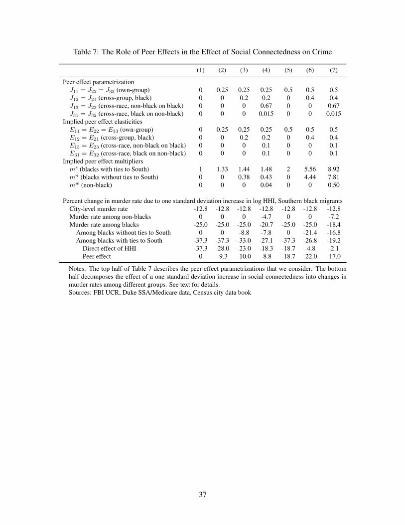
Table 7: The Role of Peer Effects in the Effect of Social Connectedness on Crime
(1) (2) (3) (4) (5) (6) (7)
Peer effect parametrizationJ11 = J22 = J33 (own-group) 0 0.25 0.25 0.25 0.5 0.5 0.5J12 = J21 (cross-group, black) 0 0 0.2 0.2 0 0.4 0.4J13 = J23 (cross-race, non-black on black) 0 0 0 0.67 0 0 0.67J31 = J32 (cross-race, black on non-black) 0 0 0 0.015 0 0 0.015
Implied peer effect elasticitiesE11 = E22 = E33 (own-group) 0 0.25 0.25 0.25 0.5 0.5 0.5E12 = E21 (cross-group, black) 0 0 0.2 0.2 0 0.4 0.4E13 = E23 (cross-race, non-black on black) 0 0 0 0.1 0 0 0.1E31 = E32 (cross-race, black on non-black) 0 0 0 0.1 0 0 0.1
Implied peer effect multipliersms (blacks with ties to South) 1 1.33 1.44 1.48 2 5.56 8.92mn (blacks without ties to South) 0 0 0.38 0.43 0 4.44 7.81mw (non-black) 0 0 0 0.04 0 0 0.50
Percent change in murder rate due to one standard deviation increase in log HHI, Southern black migrantsCity-level murder rate -12.8 -12.8 -12.8 -12.8 -12.8 -12.8 -12.8Murder rate among non-blacks 0 0 0 -4.7 0 0 -7.2Murder rate among blacks -25.0 -25.0 -25.0 -20.7 -25.0 -25.0 -18.4
Among blacks without ties to South 0 0 -8.8 -7.8 0 -21.4 -16.8Among blacks with ties to South -37.3 -37.3 -33.0 -27.1 -37.3 -26.8 -19.2
Direct effect of HHI -37.3 -28.0 -23.0 -18.3 -18.7 -4.8 -2.1Peer effect 0 -9.3 -10.0 -8.8 -18.7 -22.0 -17.0
Notes: The top half of Table 7 describes the peer effect parametrizations that we consider. The bottomhalf decomposes the effect of a one standard deviation increase in social connectedness into changes inmurder rates among different groups. See text for details.Sources: FBI UCR, Duke SSA/Medicare data, Census city data book
37

Figure 1: The Top Sending Town Accounts for Most of the Variation in Social Connectedness
Linear fit: 0.58 ( 0.02), R2 = 0.66
-6-5
-4-3
-2Lo
g H
HI,
Sou
ther
n bl
ack
mig
rant
s
-9 -8 -7 -6 -5 -4 -3 -2Leading Term of Log HHI, Southern black migrants
25,000-149,999 150,000-499,999 500,000+1980 Population
Notes: The leading term of HHI equals the log squared percent of migrants from the top sending town. Figure contains412 cities.Source: Duke SSA/Medicare data
38

Figure 2: The Effect of Social Connectedness on Murder and Motor Vehicle Theft, Robustness toControlling for 1960-1964 Crime Rate
-.6-.4
-.20
.2E
ffect
of l
og H
HI o
n m
urde
r
1960 1965 1970 1975 1980 1985 1990 1995 2000 2005Year
Model 1: baseline specification
Model 2: + control for log mean murder rate, 1960-64
(a) Murder
-.4-.2
0.2
Effe
ct o
f log
HH
I on
mot
or v
ehic
le th
eft
1960 1965 1970 1975 1980 1985 1990 1995 2000 2005Year
Model 1: baseline specification
Model 2: + control for log mean motor vehicle theft rate, 1960-64
(b) Motor Vehicle Theft
Notes: Figure shows point estimates and 95-percent confidence intervals from estimating equation (11) separately foryear 1960-64, 1965-69, and so on. Model 1 includes the same covariates used in Table 3, and model 2 additionallycontrols for the log mean crime rate from 1960-64.Sources: FBI UCR, Duke SSA/Medicare data, Census city data book
39
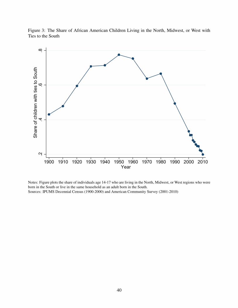
Figure 3: The Share of African American Children Living in the North, Midwest, or West withTies to the South
.2.4
.6.8
Sha
re o
f chi
ldre
n w
ith ti
es to
Sou
th
1900 1910 1920 1930 1940 1950 1960 1970 1980 1990 2000 2010Year
Notes: Figure plots the share of individuals age 14-17 who are living in the North, Midwest, or West regions who wereborn in the South or live in the same household as an adult born in the South.Sources: IPUMS Decennial Census (1900-2000) and American Community Survey (2001-2010)
40

Appendices - For Online Publication
A Theoretical Details
A.1 Proof of Proposition 1
To prove Proposition 1, we show that the assumptions of a stable equilibrium and non-negative peereffects (i.e., elements of J) imply that the peer effect multipliersms,mn, andmw are non-negative.
Let λ1, λ2, λ3 be the eigenvalues of the 3 × 3 matrix J . The spectral radius of J is defined asρ(J) ≡ max{|λ1|, |λ2|, |λ3|}. To ensure the equilibrium is stable, we assume that ρ(J) < 1. Ineach peer effect parametrization considered in Table 7, all eigenvalues are real and lie in [0, 1), andthis condition is satisfied.
The on-diagonal elements of J (J11, J22, J33) are less than one in a stable equilibrium. Thisfollows from the facts that the spectral radius is less than one if and only if limk→∞ J
k = 0 andlimk→∞ J
k = 0 implies that the on-diagonal elements of J are less than one.In a stable equilibrium, we also have that det(I − J) > 0, where I is the 3× 3 identity matrix.
This follows from our assumption that ρ(J) < 1, the fact that det(J) = λ1λ2λ3, and the fact thatdet(J) = λ1λ2λ3 if and only if det(I − J) = (1− λ1)(1− λ2)(1− λ3).
It is straightforward to show that
det(I − J) = (1− J11)[(1− J22)(1− J33)− J23J32] (A.1)− J12[J23J31 + J21(1− J33)]− J13[J21J32 + J31(1− J22)]= (1− J11)ms − J12mn − J13mw, (A.2)
where the second equality uses the peer effect multipliers defined in equations (7)-(9). Becausethe off-diagonal elements of J are non-negative (by assumption) and the on-diagonal elements ofJ are less than 1 (as implied by a stable equilibrium), we have that mn and mw are non-negative.As a result,
0 < det(I − J) ≤ (1− J11)ms. (A.3)
Because J11 < 1, this implies that ms is non-negative. QED.
B Additional Details on Sample
Our primary measure of crime is annual city-level crime counts from FBI Uniform Crime Report(UCR) data for 1960-2009. UCR data contain voluntary monthly reports on the number offensesreported to police, which we aggregate to the city-year level. These data are used regularly in theliterature and represent the best source of city crime rates. However, the UCR data are not perfect.Missing crimes are indistinguishable from true zeros in the UCR. Because cities in our samplealmost certainly experience property crime each year, we drop all city-years in which any of thethree property crimes (burglary, larceny, and motor vehicle theft) equal zero.
An alternative source of city-level crime counts is the FBI Age-Sex-Race (ASR) data, whichreport the number of offenses resulting in arrest by age, sex, and race beginning in 1980. The UCR
i
data also report the number of offenses resulting in arrest. In principle, these two data sets, whichboth rely on reports from police agencies, should lead to similar crime counts. In practice, wefound substantial differences between these data sets, especially for large cities.
Appendix Figure A.2 plots the difference between the number of murders in the FBI UCRversus ASR data by annual population. For reference, we draw a vertical line at 500,000 residentsand horizontal lines at -100 and 100. We classify each city into one of two groups, based onwhether the city has at least five “severe errors,” which define to be years in which the absolutevalue of the difference in the number of crimes is at least 100. While somewhat arbitrary, thisclassification identifies the most severe instances of disagreement between the UCR and ASRdata.
There are six cities with at least five severe errors: Chicago, Detroit, Los Angeles, Milwaukee,New York, and Philadelphia. Appendix Figure A.3 plots the number of murders from the UCR andASR data over time. There does not appear to be a simple explanation for the differences betweenthe two data sets. As a result, we drop these six cities from our main analysis sample. However,as seen in Panel A of Appendix Table A.10, our results are similar when we include these largecities.44
C Additional Details on Variation in Social Connectedness
Appendix Table A.5 examines the correlation between log HHI and several demographic and eco-nomic covariates. In particular, we regress log HHI on various covariates for the 236 cities ob-served in every decade from 1960 to 2000. To facilitate comparisons, we normalize all variables,separately for each decade, to have mean zero and standard deviation one. Only the log numberof migrants and the manufacturing employment share are consistently correlated with log HHI.The negative correlation between log HHI and the log number of migrants arises because a largenumber of migrants necessarily came from many sending towns, due to the small size of Southerntowns relative to Northern cities. The positive correlation between log HHI and the manufactur-ing employment share arises because social interactions in location decisions guided migrants todestinations with higher manufacturing employment, which was especially attractive to AfricanAmerican workers (Stuart and Taylor, 2017). Appendix Table A.6 shows results when adding anumber of covariates measured among African-Americans.45
Appendix Figure A.4 further describes the cross-city variation in social connectedness by plot-ting log HHI and the log number of Southern black migrants. Our regressions identify the effect ofsocial connectedness on crime with variation in log HHI conditional on the log number of migrantsin a city (and other covariates), which is variation in the vertical dimension of Figure A.4. Thereis considerable variation in log HHI conditional on the log number of migrants.
44Mosher, Miethe and Hart (2011) discuss measurement error in the UCR data in detail, but do not discuss thediscrepancies we have identified between the UCR and ASR data.
45African American covariates include percent age 5-17, 18-64, and 65+, percent female, percent with a high schooldegree, percent with a college degree, and the unemployment rate. These variables are not available for 1960. In 1990,only the education variables are available; for the other variables, we linearly interpolate the 1980 and 2000 values.
ii

D Estimating a Model of Social Interactions in Location Decisions
Appendix D describes a structural model of social interactions in location decisions. This model al-lows us to estimate the share of migrants that chose their destination because of social interactions.We include this variable in our regressions to examine whether the effect of social connectednessis driven by variation across cities in unobserved characteristics of migrants.
D.1 Model of Social Interactions in Location Decisions
Migrants from birth town j are indexed on a circle by i ∈ {1, . . . , Nj}, whereNj is the total numberof migrants from town j. For migrant i, destination k belongs to one of three preference groups:high (Hi), medium (Mi), or low (Li). The high preference group contains a single destination. Inthe absence of social interactions, the destination in Hi is most preferred, and destinations in Mi
are preferred over those in Li.46 A migrant never moves to a destination in Li. A migrant choosesa destination in Mi if and only if his neighbor, i − 1, chooses the same destination. A migrantchooses a destination in Hi if his neighbor chooses the same destination or his neighbor selects adestination in Li.47
Migrants from the same birth town can differ in their preferences over destinations. The prob-ability that destination k is in the high preference group for a migrant from town j is hj,k ≡P[k ∈ Hi|i ∈ j], and the probability that destination k is in the medium preference group ismj,k ≡ P[k ∈Mi|i ∈ j].
Migrants with many destinations in their medium preference group will tend to be influencedby the decisions of other migrants. For estimating the effect of social connectedness on crime,distinguishing between types of migrants is important because migrants that are more influencedby social interactions might differ along several dimensions. For example, migrants with manydestinations in their medium preference group might be negatively selected in terms of earningsability or be more pro-social, and these characteristics might bias estimates of δ is equation (11).
The probability that migrant i moves to destination k given that his neighbor moves there is
ρj,k ≡ P[Di,j,k = 1|Di−1,j,k = 1, i ∈ j] = P[k ∈ Hi|i ∈ j] + P[k ∈Mi|i ∈ j] (A.4)= hj,k +mj,k, (A.5)
where Di,j,k equals one if migrant i moves from j to k and zero otherwise.The probability that destination k is in the medium preference group, conditional on not being
in the high preference group, is νj,k ≡ P[k ∈ Mi|k /∈ Hi, i ∈ j]. The conditional probabilitydefinition for νj,k implies that mj,k = νj,k(1 − hj,k). We use νj,k to derive a simple sequentialestimation approach.
46The assumption that Hi is a non-empty singleton ensures that migrant i has a well-defined location decision inthe absence of social interactions. We could allow Hi to contain many destinations and specify a decision rule amongthe elements of Hi. This extension would complicate the model without adding any new insights.
47This model shares a similar structure as Glaeser, Sacerdote and Scheinkman (1996) in that some agents imitatetheir neighbors. However, we differ from Glaeser, Sacerdote and Scheinkman (1996) in that we model the interdepen-dence between various destinations (i.e., this is a multinomial choice problem) and allow for more than two types ofagents.
iii
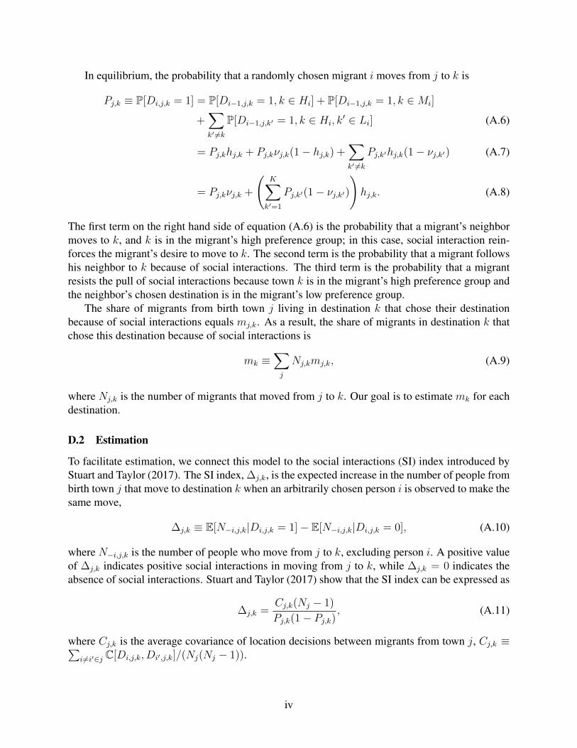
In equilibrium, the probability that a randomly chosen migrant i moves from j to k is
Pj,k ≡ P[Di,j,k = 1] = P[Di−1,j,k = 1, k ∈ Hi] + P[Di−1,j,k = 1, k ∈Mi]
+∑k′ 6=k
P[Di−1,j,k′ = 1, k ∈ Hi, k′ ∈ Li] (A.6)
= Pj,khj,k + Pj,kνj,k(1− hj,k) +∑k′ 6=k
Pj,k′hj,k(1− νj,k′) (A.7)
= Pj,kνj,k +
(K∑k′=1
Pj,k′(1− νj,k′)
)hj,k. (A.8)
The first term on the right hand side of equation (A.6) is the probability that a migrant’s neighbormoves to k, and k is in the migrant’s high preference group; in this case, social interaction rein-forces the migrant’s desire to move to k. The second term is the probability that a migrant followshis neighbor to k because of social interactions. The third term is the probability that a migrantresists the pull of social interactions because town k is in the migrant’s high preference group andthe neighbor’s chosen destination is in the migrant’s low preference group.
The share of migrants from birth town j living in destination k that chose their destinationbecause of social interactions equals mj,k. As a result, the share of migrants in destination k thatchose this destination because of social interactions is
mk ≡∑j
Nj,kmj,k, (A.9)
where Nj,k is the number of migrants that moved from j to k. Our goal is to estimate mk for eachdestination.
D.2 Estimation
To facilitate estimation, we connect this model to the social interactions (SI) index introduced byStuart and Taylor (2017). The SI index, ∆j,k, is the expected increase in the number of people frombirth town j that move to destination k when an arbitrarily chosen person i is observed to make thesame move,
∆j,k ≡ E[N−i,j,k|Di,j,k = 1]− E[N−i,j,k|Di,j,k = 0], (A.10)
where N−i,j,k is the number of people who move from j to k, excluding person i. A positive valueof ∆j,k indicates positive social interactions in moving from j to k, while ∆j,k = 0 indicates theabsence of social interactions. Stuart and Taylor (2017) show that the SI index can be expressed as
∆j,k =Cj,k(Nj − 1)
Pj,k(1− Pj,k), (A.11)
where Cj,k is the average covariance of location decisions between migrants from town j, Cj,k ≡∑i 6=i′∈j C[Di,j,k, Di′,j,k]/(Nj(Nj − 1)).
iv

The model implies that Cj,k equals48
Cj,k =2Pj,k(1− Pj,k)
∑Nj−1s=1 (Nj − s)
(ρj,k−Pj,k
1−Pj,k
)sNj(Nj − 1)
. (A.12)
Substituting equation (A.12) into equation (A.11) and simplifying yields49
∆j,k =2(ρj,k − Pj,k)
1− ρj,k, (A.13)
which can be rearranged to show that
ρj,k =2Pj,k + ∆j,k
2 + ∆j,k
. (A.14)
We follow the approach described in Stuart and Taylor (2017) to estimate Pj,k and ∆j,k usinginformation on migrants’ location decisions from the Duke SSA/Medicare data.50 We then useequation (A.14) to estimate ρj,k with our estimates of Pj,k and ∆j,k.
Equations (A.5) and (A.8), plus the fact that mj,k = νj,k(1− hj,k), imply that
ρj,k = νj,k +Pj,k(1− νj,k)2∑Kk′=1 Pj,k′(1− νj,k′)
. (A.15)
We use equation (A.15) to estimate νj ≡ (νj,1, . . . , νj,K) using our estimates of (Pj,1, . . . , Pj,K ,ρj,1, . . . , ρj,K). We employ a computationally efficient algorithm that leverages the fact that equa-tion (A.15) is a quadratic equation in νj,k, conditional on
∑Kk′=1 Pj,k′(1−νj,k′). We initially assume
that∑K
k′=1 Pj,k′(1− νj,k′) =∑K
k′=1 Pj,k′ = 1, then solve for νj,k using the quadratic formula, thenconstruct an updated estimate of
∑Kk′=1 Pj,k′(1 − νj,k′), and then solve again for νj,k using the
quadratic formula. We require that each estimate of νj,k lies in [0, 1]. This iterated algorithmconverges very rapidly in the vast majority of cases.51
We use equation (A.8) to estimate hj,k with our estimates of ρj,k and νj,k. Finally, we estimatemj,k using the fact that mj,k = ρj,k − hj,k. We use equation (A.9) to estimate our parameter ofinterest, mk, using estimates of mj,k and observed migration flows, Nj,k.
48This follows from the fact that the covariance of location decisions for individuals i and i + n isC[Di,j,k, Di+n,j,k] = Pj,k(1− Pj,k)
(ρj,k−Pj,k
1−Pj,k
)n.
49Equation (A.13) results from taking the limit as Nj →∞, and so relies on Nj being sufficiently large.50We use cross validation to define birth town groups. See Stuart and Taylor (2017) for details.51For 10 birth towns, the algorithm does not converge because our estimates of Pj,k and ρj,k do not yield a real
solution to the quadratic formula. We examined the sensitivity of our results to these cases by (1) dropping birth townsfor which the algorithm did not converge, (2) estimating νj,k and
∑Kk′=1 Pj,k′(1− νj,k′) as the average of the values
in the final four iterations, and (3) forcing νj,k to equal zero for any (j, k) observation for which the quadratic formulasolution does not exist. The motivation for (3) is that our estimates of Pj,k and ρj,k in these 10 cases were consistentwith negative values of νj,k, even though this is not a feasible solution. All three options yielded nearly identicalestimates of our variable of interest, mk. This is not surprising because these 10 birth towns account for a negligibleshare of the over 5,000 birth towns used to estimate mk.
v

D.3 Results
Appendix Figure A.5 displays a histogram of our estimates of the share of migrants that chose theirdestination because of social interactions, mk, for cities in the North, Midwest, and West regions.The estimates range from 0 to 0.62. The unweighted average of mk across cities is 0.26, and the1980 population weighted average is 0.39.
Appendix Table A.9 examines the relationship between log HHI, the log number of migrants,and mk. The raw correlation between log HHI and mk is negative, but when we control for the lognumber of migrants, log HHI and mk are positively correlated, as expected. This relationship issimilar when including state fixed effects.
Appendix Figure A.6 further describes the relationship between log HHI and mk. Panel Aplots the unconditional relationship between log HHI and mk, while Panel B plots the relationshipconditional on the log number of migrants.52 When we control formk in equation (11), we identifythe effect of social connectedness on crime using variation in the vertical dimension of Panel B.
Conditional on the number of migrants in a destination and the share of migrants that chosetheir destination because of social interactions, variation in social connectedness continues to arisefrom concentrated birth town to destination city population flows. To see this, consider two hy-pothetical cities that each have 20 migrants, one-fourth of whom chose their destination becauseof social interactions. In the low HHI city, the 20 migrants come from five birth towns. Eachtown sends four migrants, one of whom moves there because of social interactions. As a result,HHILow = 0.2. In the high HHI city, the 20 migrants also come from five birth towns. One townsends 12 migrants, three of whom move there because of social interactions. Two towns each sendtwo migrants, one of whom moves there because of social interactions, and two towns each sendtwo migrants, neither of whom is influenced by social interactions. As a result, HHIHigh = 0.4.53
This example is consistent with Figure 1 in that variation in social connectedness arises from thetop sending town.
The structural model features local social interactions: each migrant directly influences nomore than one migrant.54 As a result, the model does not distinguish between the case where 12migrants come from one town, with three migrants influenced by social interactions, and the casewhere 12 migrants come from three towns, with three migrants influenced by social interactions.Although this model does not capture all possible forms of social interactions, we believe that itlikely captures the most relevant threats to the empirical strategy for this paper.
E Details on Peer Effect Parametrization
Appendix E provides additional details on the literature that guides our parametrization of peereffects in Section 5.4.
Case and Katz (1991) find that a one percent increase in the neighborhood crime rate leads to a0.1 percent increase in a Boston youth’s self-reported propensity of committing a crime during thelast year (Table 10). This implies that a one percentage point increase in the neighborhood crime
52In particular, Panel B plots the residuals from regressing log HHI and mk on the log number of migrants.53Alternatively, suppose that in the high HHI city, the 20 migrants come from three birth towns. One town sends
12 migrants, three of whom move there because of social interactions, and two towns each send four migrants, one ofwhom moves there because of social interactions. As a result, HHIHigh = 0.44.
54However, a single migrant can indirectly influence several migrants.
vi
rate leads to a 0.1 percentage point increase in youth’s crime rate, suggesting on-diagonal elementsof J close to 0.1.
Glaeser, Sacerdote and Scheinkman (1996) estimate a local social interactions model in whichthere are two types of agents. Fixed agents are not affected by their peers, and compliers imitatetheir neighbor. The probability that an agent is a complier thus maps to the on-diagonal elements ofJ . In Table IIA, the authors report estimates of f(π) = (2−π)/π, where π is the probability that anagent is a fixed type. The probability that an agent is a complier is 1−π = 1−2/(1+f(π)). UsingFBI UCR data on murders across cities for 1970 and 1985, Glaeser, Sacerdote and Scheinkman(1996) report estimates of f(π) between 2 and 4.5, implying on-diagonal elements of J between1/3 and 2/3. For robbery and motor vehicle theft, the authors estimate f(π) in the range of 37-155and 141-382, suggesting diagonal elements of J very close to 1.
Ludwig and Kling (2007) find no evidence that neighborhood violent crime rates affect violentcrime arrests among MTO participants age 15-25 (Table 4). These estimates suggest on-diagonalelements of J close to zero.
Damm and Dustmann (2014) estimate the effect of municipality crime rates on refugees’ crim-inal convictions in Denmark. For males, they find that a one percentage point increase in themunicipality crime rate leads to a 7-13 percent increase in the probability of conviction over aseven year period from ages 15-21 (Table 3, also see p. 1820). Given an average conviction rateof 46 percent, this translates into a 3-6 percentage point increase in the probability of conviction;we take the midpoint of 4.5. For females, the municipality crime rate has no effect on convictions.Consequently, these estimates imply that a one percentage point increase in the municipality crimerate leads to a (0.5 · 4.5)/7 ≈ 0.32 percentage point increase in refugees’ annual conviction rate.This suggests on-diagonal elements of J close to 1/3. Damm and Dustmann (2014) find that, be-yond the impact of the municipality crime rate, the crime rate of co-nationals has an additionalimpact while the crime rate of immigrants from other countries does not (Table 7). This suggeststhat cross-group peer effects might be small.
In sum, estimates from Case and Katz (1991) suggest on-diagonal values of J close to 0.1,estimates from Glaeser, Sacerdote and Scheinkman (1996) suggest on-diagonal elements of Jclose to 0.5 for murder, estimates from Ludwig and Kling (2007) suggest on-diagonal elements ofJ close to zero, and estimates from Damm and Dustmann (2014) suggest on-diagonal values of Jclose to 0.3 and off-diagonal elements near zero.
vii

Table A.1: Summary Statistics: Crime and Social Connectedness, 1960-2009
First Third FractionMean SD Quartile Quartile Zero
Offenses reported to police per 100,000 residentsMurder 6.8 8.9 1.8 8.9 0.181Rape 30 28 10 40 0.069Robbery 219 255 69 277 0.003Assault 1,137 1,099 287 1,629 0.005Burglary 1,241 844 675 1,642 0.000Larceny 3,234 1,776 2,032 4,204 0.000Motor Vehicle Theft 594 526 264 757 0.000
Population 105,807 132,412 39,796 108,034 -HHI, Southern Black Migrants 0.019 0.016 0.007 0.028 -Log HHI, Southern Black Migrants -4.244 0.792 -4.923 -3.591 -Top Sending Town Share, Southern Black Migrants 0.061 0.041 0.036 0.073 -Number, Southern Black Migrants 742 1,679 60 650 -
Notes: Each observation is a city-year. HHI and migrant counts are calculated among all individuals bornin the former Confederacy states from 1916-1936. Data on rape is only available starting in 1964. Sampleis restricted to cities with less than 500,000 residents in 1980.Sources: FBI UCR, Duke SSA/Medicare dataset
viii

Table A.2: Summary Statistics: Cities’ Average Crime Rates
Percentile
Mean SD 5 25 50 75 95
Murder 6.8 6.8 1.3 2.7 4.6 8.3 19.6Rape 29.5 18.6 6.5 16.2 26.5 37.6 66.6Robbery 217.1 186.5 42.2 93.7 157.3 273.0 632.9Assault 1,124.8 623.3 326.7 652.8 1,019.4 1,471.9 2,320.4Burglary 1,239.6 473.3 544.0 895.2 1,189.0 1,534.1 2,095.9Larceny 3,227.1 1,205.0 1,525.6 2,383.6 3,186.4 3,927.1 5,030.8Motor Vehicle Theft 588.7 381.9 178.7 314.5 464.5 761.9 1,328.9
Notes: For each city, we construct an average crime rate across years 1960-2009. Table A.2 reports summarystatistics of these average crime rates. Sample is restricted to cities with less than 500,000 residents in 1980.Sources: FBI UCR
ix

Table A.3: Summary Statistics: Cities With and Without 1911-1916 Murder Rates
1911-1916 Murder Rates Observed
Yes No(1) (2)
HHI, Southern black migrants 0.007 0.021(0.006) (0.016)
Number, Southern black migrants 7,999 540(16,068) (2,079)
Population, 1980 549,344 80,839(1,099,422) (170,680)
Percent black, 1980 0.237 0.103(0.152) (0.148)
Percent age 5-17, 1980 0.187 0.196(0.0291) (0.0324)
Percent age 18-64, 1980 0.605 0.621(0.0280) (0.0422)
Percent age 65+, 1980 0.136 0.112(0.0223) (0.0383)
Percent female, 1980 0.530 0.519(0.008) (0.019)
Percent 25+ with HS, 1980 0.489 0.560(0.080) (0.098)
Percent 25+ with College, 1980 0.118 0.137(0.048) (0.078)
Log area, square miles, 1980 3.886 2.729(0.986) (0.888)
Log median family income, 1979 10.85 11.06(0.148) (0.205)
Unemployment rate, 1980 0.0886 0.0708(0.033) (0.030)
Labor force participation rate, 1980 0.458 0.483(0.041) (0.052)
Manufacturing emp. share, 1980 0.213 0.233(0.072) (0.094)
N (cities) 46 369
Notes: Table reports means and, in parentheses, standard deviations. Column 1 containscities in the North, Midwest, and West regions that are in our main analysis sample andfor which we observe murder rates for at least one year from 1911-1916. These citieshave at least 100,000 residents in 1920 and at least 5 deaths each year. Column 2contains cities in the North, Midwest, and West regions that are in our main analysissample but for which we do not observe homicide rates from 1911-1916.Sources: Census (1922, p. 64-65) , Duke SSA/Medicare data, Census city data book
x

Table A.4: The Relationship between Social Connectedness and Measures of Social Capital
Dependent variable: Log HHI, Southern black migrants(1) (2) (3) (4) (5) (6) (7) (8)
Panel A: All CitiesAssociational density 0.0708 0.103** 0.110 0.135**
(0.0574) (0.0479) (0.0922) (0.0589)Social capital index 0.0432 0.0418 -0.0480 -0.0513
(0.0568) (0.0459) (0.0941) (0.0554)Social capital composite index 0.0342 0.0308
(0.0557) (0.0428)Log number, Southern black migrants -0.867*** -0.866*** -0.866*** -0.867***
(0.0289) (0.0287) (0.0287) (0.0293)State fixed effects x x x xR2 0.007 0.741 0.002 0.739 0.001 0.740 0.008 0.742N (cities) 484 484 484 484 484 484 484 484Counties 225 225 225 225 225 225 225 225
Panel B: Cities with Above Median Black Population Share in 1990Associational density 0.313*** 0.145* 0.509*** 0.179*
(0.0644) (0.0742) (0.103) (0.0964)Social capital index 0.197*** 0.103 -0.257*** -0.0556
(0.0587) (0.0725) (0.0968) (0.0839)Social capital composite index 0.176*** 0.0847
(0.0571) (0.0678)Log number, Southern black migrants -0.674*** -0.695*** -0.696*** -0.669***
(0.0502) (0.0485) (0.0486) (0.0507)State fixed effects x x x xR2 0.129 0.598 0.043 0.591 0.034 0.590 0.155 0.603N (cities) 226 226 226 226 226 226 226 226Counties 151 151 151 151 151 151 151 151
Notes: All variables are normalized to have mean zero and standard deviation one in the sample used in Panel A. See Rupasingha and Goetz(2008) for definitions of associational density and social capital indices, which are measured at the county level using data from 1988 and 1990.The correlation between the social capital index and the social capital composite index is 0.998. Panel B has less than half the observations asPanel A because percent black in 1990 is missing for some cities. Standard errors, clustered at the county level, are in parentheses. * p < 0.1;** p < 0.05; *** p < 0.01Sources: Duke SSA/Medicare data, Rupasingha and Goetz (2008)
xi
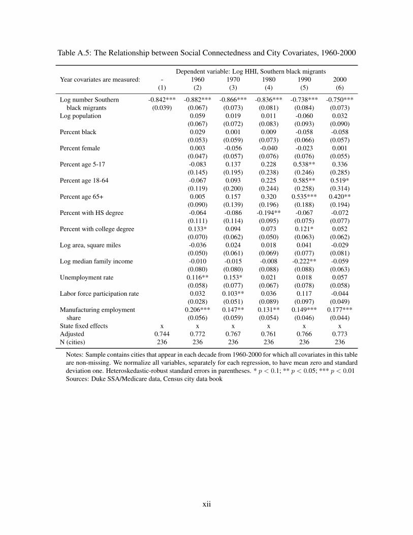
Table A.5: The Relationship between Social Connectedness and City Covariates, 1960-2000
Dependent variable: Log HHI, Southern black migrantsYear covariates are measured: - 1960 1970 1980 1990 2000
(1) (2) (3) (4) (5) (6)
Log number Southern -0.842*** -0.882*** -0.866*** -0.836*** -0.738*** -0.750***black migrants (0.039) (0.067) (0.073) (0.081) (0.084) (0.073)
Log population 0.059 0.019 0.011 -0.060 0.032(0.067) (0.072) (0.083) (0.093) (0.090)
Percent black 0.029 0.001 0.009 -0.058 -0.058(0.053) (0.059) (0.073) (0.066) (0.057)
Percent female 0.003 -0.056 -0.040 -0.023 0.001(0.047) (0.057) (0.076) (0.076) (0.055)
Percent age 5-17 -0.083 0.137 0.228 0.538** 0.336(0.145) (0.195) (0.238) (0.246) (0.285)
Percent age 18-64 -0.067 0.093 0.225 0.585** 0.519*(0.119) (0.200) (0.244) (0.258) (0.314)
Percent age 65+ 0.005 0.157 0.320 0.535*** 0.420**(0.090) (0.139) (0.196) (0.188) (0.194)
Percent with HS degree -0.064 -0.086 -0.194** -0.067 -0.072(0.111) (0.114) (0.095) (0.075) (0.077)
Percent with college degree 0.133* 0.094 0.073 0.121* 0.052(0.070) (0.062) (0.050) (0.063) (0.062)
Log area, square miles -0.036 0.024 0.018 0.041 -0.029(0.050) (0.061) (0.069) (0.077) (0.081)
Log median family income -0.010 -0.015 -0.008 -0.222** -0.059(0.080) (0.080) (0.088) (0.088) (0.063)
Unemployment rate 0.116** 0.153* 0.021 0.018 0.057(0.058) (0.077) (0.067) (0.078) (0.058)
Labor force participation rate 0.032 0.103** 0.036 0.117 -0.044(0.028) (0.051) (0.089) (0.097) (0.049)
Manufacturing employment 0.206*** 0.147** 0.131** 0.149*** 0.177***share (0.056) (0.059) (0.054) (0.046) (0.044)
State fixed effects x x x x x xAdjusted 0.744 0.772 0.767 0.761 0.766 0.773N (cities) 236 236 236 236 236 236
Notes: Sample contains cities that appear in each decade from 1960-2000 for which all covariates in this tableare non-missing. We normalize all variables, separately for each regression, to have mean zero and standarddeviation one. Heteroskedastic-robust standard errors in parentheses. * p < 0.1; ** p < 0.05; *** p < 0.01Sources: Duke SSA/Medicare data, Census city data book
xii

Table A.6: The Relationship between Social Connectedness and City Covariates, 1960-2000, In-cluding African American Specific Covariates
Dependent variable: Log HHI, Southern black migrantsYear covariates are measured: 1970 1980 1990 2000
(1) (2) (3) (4)
Log number Southern black migrants -0.837*** -0.799*** -0.750*** -0.781***(0.070) (0.078) (0.090) (0.098)
Log population 0.025 0.038 -0.008 0.061(0.079) (0.085) (0.096) (0.097)
Percent black -0.006 0.011 -0.036 -0.063(0.058) (0.074) (0.071) (0.065)
Percent female -0.087 -0.006 -0.013 0.036(0.059) (0.078) (0.089) (0.075)
Percent age 5-17 -0.031 0.217 0.447* 0.499(0.215) (0.256) (0.264) (0.322)
Percent age 18-64 -0.086 0.257 0.509* 0.645*(0.224) (0.268) (0.276) (0.355)
Percent age 65+ 0.054 0.300 0.449** 0.491**(0.155) (0.212) (0.205) (0.215)
Percent with HS degree 0.039 -0.133 -0.009 -0.029(0.129) (0.104) (0.090) (0.100)
Percent with college degree 0.025 0.007 -0.011 -0.023(0.071) (0.053) (0.081) (0.084)
Log area, square miles 0.018 -0.036 -0.008 -0.035(0.063) (0.074) (0.081) (0.086)
Log median family income -0.059 -0.019 -0.185* -0.054(0.091) (0.086) (0.097) (0.080)
Unemployment rate 0.182** -0.027 -0.059 0.025(0.081) (0.084) (0.090) (0.055)
Labor force participation rate 0.092* 0.020 0.091 -0.037(0.051) (0.087) (0.103) (0.054)
Manufacturing employment share 0.182*** 0.155*** 0.153*** 0.181***(0.063) (0.057) (0.051) (0.046)
African American-Specific Covariates:Percent female 0.032 -0.088 -0.003 0.075
(0.044) (0.060) (0.073) (0.071)Percent age 5-17 0.122 0.099 0.144 -0.139
(0.076) (0.112) (0.150) (0.171)Percent age 18-64 0.134 0.042 0.194 -0.058
(0.085) (0.128) (0.177) (0.207)Percent age 65+ 0.046 0.053 0.100 -0.015
(0.054) (0.068) (0.087) (0.103)Percent with HS degree -0.188** -0.075 -0.113 -0.036
(0.074) (0.072) (0.075) (0.071)Percent with college degree 0.146*** 0.119* 0.124 0.062
(0.052) (0.064) (0.078) (0.077)Unemployment rate -0.080* 0.053 0.111* 0.105***
(0.046) (0.072) (0.059) (0.040)State fixed effects x x x xAdjusted R2 0.775 0.762 0.767 0.777N (cities) 236 236 236 236
Notes: African American-specific covariates are not available for 1960. See note to Table A.5.Sources: Duke SSA/Medicare data, Census city data book
xiii
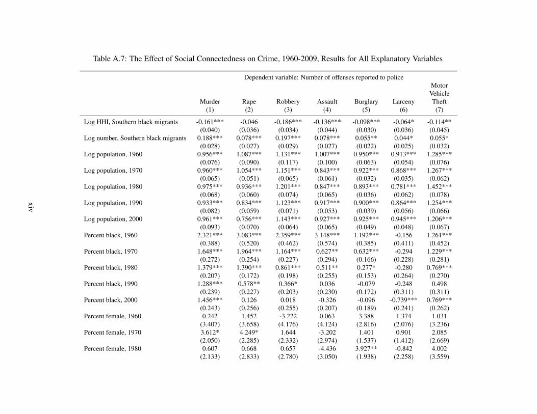
Table A.7: The Effect of Social Connectedness on Crime, 1960-2009, Results for All Explanatory Variables
Dependent variable: Number of offenses reported to policeMotorVehicle
Murder Rape Robbery Assault Burglary Larceny Theft(1) (2) (3) (4) (5) (6) (7)
Log HHI, Southern black migrants -0.161*** -0.046 -0.186*** -0.136*** -0.098*** -0.064* -0.114**(0.040) (0.036) (0.034) (0.044) (0.030) (0.036) (0.045)
Log number, Southern black migrants 0.188*** 0.078*** 0.197*** 0.078*** 0.055** 0.044* 0.055*(0.028) (0.027) (0.029) (0.027) (0.022) (0.025) (0.032)
Log population, 1960 0.956*** 1.087*** 1.131*** 1.007*** 0.950*** 0.913*** 1.285***(0.076) (0.090) (0.117) (0.100) (0.063) (0.054) (0.076)
Log population, 1970 0.960*** 1.054*** 1.151*** 0.843*** 0.922*** 0.868*** 1.267***(0.065) (0.051) (0.065) (0.061) (0.032) (0.035) (0.062)
Log population, 1980 0.975*** 0.936*** 1.201*** 0.847*** 0.893*** 0.781*** 1.452***(0.068) (0.060) (0.074) (0.065) (0.036) (0.062) (0.078)
Log population, 1990 0.933*** 0.834*** 1.123*** 0.917*** 0.900*** 0.864*** 1.254***(0.082) (0.059) (0.071) (0.053) (0.039) (0.056) (0.066)
Log population, 2000 0.961*** 0.756*** 1.143*** 0.927*** 0.925*** 0.945*** 1.206***(0.093) (0.070) (0.064) (0.065) (0.049) (0.048) (0.067)
Percent black, 1960 2.321*** 3.083*** 2.359*** 3.148*** 1.192*** -0.156 1.261***(0.388) (0.520) (0.462) (0.574) (0.385) (0.411) (0.452)
Percent black, 1970 1.648*** 1.964*** 1.164*** 0.627** 0.632*** -0.294 1.229***(0.272) (0.254) (0.227) (0.294) (0.166) (0.228) (0.281)
Percent black, 1980 1.379*** 1.390*** 0.861*** 0.511** 0.277* -0.280 0.769***(0.207) (0.172) (0.198) (0.255) (0.153) (0.264) (0.270)
Percent black, 1990 1.288*** 0.578** 0.366* 0.036 -0.079 -0.248 0.498(0.239) (0.227) (0.203) (0.230) (0.172) (0.311) (0.311)
Percent black, 2000 1.456*** 0.126 0.018 -0.326 -0.096 -0.739*** 0.769***(0.243) (0.256) (0.255) (0.207) (0.189) (0.241) (0.262)
Percent female, 1960 0.242 1.452 -3.222 0.063 3.388 1.374 1.031(3.407) (3.658) (4.176) (4.124) (2.816) (2.076) (3.236)
Percent female, 1970 3.612* 4.249* 1.644 -3.202 1.401 0.901 2.085(2.050) (2.285) (2.332) (2.974) (1.537) (1.412) (2.669)
Percent female, 1980 0.607 0.668 0.657 -4.436 3.927** -0.842 4.002(2.133) (2.833) (2.780) (3.050) (1.938) (2.258) (3.559)
xiv

Table A.7: The Effect of Social Connectedness on Crime, 1960-2009, Results for All Explanatory Variables
Dependent variable: Number of offenses reported to policeMotorVehicle
Murder Rape Robbery Assault Burglary Larceny Theft(1) (2) (3) (4) (5) (6) (7)
Percent female, 1990 -5.433** -0.834 -0.291 -1.489 1.076 -1.322 3.778(2.760) (2.924) (3.308) (2.375) (2.211) (2.246) (3.911)
Percent female, 2000 4.053 -0.389 -1.803 2.341 -2.511 -1.030 -3.326(3.746) (2.664) (3.099) (2.325) (2.173) (2.108) (3.098)
Percent age 5-17, 1960 4.090 -12.179** 6.624 -4.568 -2.561 -9.611** 1.920(5.280) (5.210) (6.683) (6.893) (4.229) (4.067) (4.623)
Percent age 18-64, 1960 1.442 -13.519*** 5.041 -1.187 -5.166 -9.784*** 0.784(3.648) (4.149) (4.145) (4.876) (3.185) (2.912) (3.284)
Percent age 65+, 1960 -0.897 -12.557*** 2.215 -9.096** -4.374 -8.573*** -4.108(3.238) (3.909) (4.772) (4.348) (3.030) (2.617) (3.310)
Percent age 5-17, 1970 -5.454* -11.591*** -7.378** -9.470** -5.736*** -5.050** -1.159(3.152) (2.967) (3.103) (4.491) (2.037) (2.304) (3.276)
Percent age 18-64, 1970 -2.513 -7.947*** -3.592 -9.527** -6.683*** -5.284*** 2.039(2.814) (2.631) (2.636) (4.310) (1.820) (2.035) (2.734)
Percent age 65+, 1970 -4.309* -10.748*** -5.395** -6.652** -5.116*** -4.239** -2.523(2.517) (2.359) (2.459) (3.169) (1.668) (1.705) (2.685)
Percent age 5-17, 1980 -12.343*** -13.613*** -8.390** -16.949*** -9.971*** -2.246 7.411*(3.438) (3.245) (4.121) (4.793) (2.607) (4.333) (4.480)
Percent age 18-64, 1980 -11.264*** -10.875*** -6.944** -14.628*** -8.401*** -2.193 9.454***(2.666) (2.486) (3.176) (3.460) (1.877) (2.546) (3.444)
Percent age 65+, 1980 -8.755*** -10.386*** -5.146 -10.542*** -7.288*** -0.331 6.087(2.787) (2.754) (3.397) (3.800) (1.944) (3.987) (3.892)
Percent age 5-17, 1990 -17.106*** -13.983*** -11.102*** -8.701** -9.031*** 0.635 -1.025(4.958) (4.238) (3.917) (4.136) (2.896) (3.216) (4.776)
Percent age 18-64, 1990 -16.182*** -10.698*** -8.172*** -8.045*** -10.217*** -0.423 0.254(3.203) (2.952) (2.739) (2.998) (2.090) (2.428) (3.189)
Percent age 65+, 1990 -12.205*** -10.496*** -7.097** -6.718** -7.550*** 1.355 -0.501(3.600) (3.203) (2.835) (3.101) (2.104) (2.216) (3.452)
Percent age 5-17, 2000 -5.758 -12.822** -4.488 -1.759 1.393 0.675 4.214(6.000) (5.300) (4.663) (4.404) (4.506) (4.279) (5.517)
xv
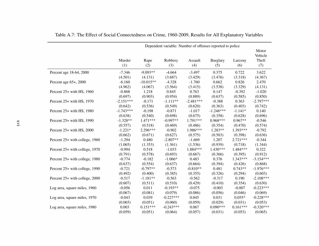
Table A.7: The Effect of Social Connectedness on Crime, 1960-2009, Results for All Explanatory Variables
Dependent variable: Number of offenses reported to policeMotorVehicle
Murder Rape Robbery Assault Burglary Larceny Theft(1) (2) (3) (4) (5) (6) (7)
Percent age 18-64, 2000 -7.346 -9.093** -4.664 -3.497 0.375 0.722 3.622(4.501) (4.131) (3.687) (3.429) (3.476) (3.318) (4.367)
Percent age 65+, 2000 -6.160 -10.015** -4.328 -1.760 0.662 0.826 2.470(4.962) (4.067) (3.564) (3.415) (3.538) (3.329) (4.131)
Percent 25+ with HS, 1960 -0.868 1.218 0.845 0.763 0.147 -0.392 -1.020(0.697) (0.903) (0.954) (0.889) (0.637) (0.585) (0.850)
Percent 25+ with HS, 1970 -2.151*** -0.171 -1.111** -2.481*** -0.388 0.363 -2.797***(0.642) (0.536) (0.549) (0.620) (0.363) (0.403) (0.742)
Percent 25+ with HS, 1980 -1.743*** -0.198 -0.871 -1.017 -1.246*** -1.141* 0.140(0.638) (0.540) (0.698) (0.675) (0.358) (0.628) (0.696)
Percent 25+ with HS, 1990 -1.328** 1.471*** -0.997** 1.791*** 0.968*** 0.967** -0.546(0.557) (0.518) (0.469) (0.486) (0.354) (0.470) (0.574)
Percent 25+ with HS, 2000 -1.221* 2.296*** -0.902 1.986*** 1.283** 1.393*** -0.792(0.662) (0.671) (0.627) (0.575) (0.503) (0.398) (0.636)
Percent 25+ with college, 1960 -1.294 0.480 -2.807** -1.669 1.207 2.721*** -0.344(1.065) (1.353) (1.361) (1.536) (0.939) (0.718) (1.344)
Percent 25+ with college, 1970 -0.994 0.518 -1.033 1.884*** 1.430*** 1.484*** 0.322(0.791) (0.578) (0.693) (0.667) (0.366) (0.395) (0.912)
Percent 25+ with college, 1980 -0.774 -0.182 -1.066* 0.483 0.376 1.343*** -3.154***(0.637) (0.554) (0.637) (0.664) (0.394) (0.426) (0.868)
Percent 25+ with college, 1990 -0.721 -0.797** -0.573 -0.810** 0.481 0.743** -1.976***(0.492) (0.400) (0.385) (0.355) (0.326) (0.294) (0.603)
Percent 25+ with college, 2000 -0.517 -1.181** -0.563 -0.562 -0.317 0.190 -2.108***(0.607) (0.511) (0.510) (0.429) (0.410) (0.354) (0.630)
Log area, square miles, 1960 -0.056 0.011 -0.193** -0.075 -0.003 -0.007 -0.223***(0.067) (0.081) (0.079) (0.086) (0.056) (0.046) (0.069)
Log area, square miles, 1970 -0.043 0.039 -0.227*** 0.045 0.031 0.055* -0.228***(0.065) (0.051) (0.060) (0.059) (0.029) (0.031) (0.053)
Log area, square miles, 1980 0.003 0.151*** -0.243*** 0.067 0.090*** 0.161*** -0.320***(0.059) (0.051) (0.064) (0.057) (0.031) (0.053) (0.065)
xvi

Table A.7: The Effect of Social Connectedness on Crime, 1960-2009, Results for All Explanatory Variables
Dependent variable: Number of offenses reported to policeMotorVehicle
Murder Rape Robbery Assault Burglary Larceny Theft(1) (2) (3) (4) (5) (6) (7)
Log area, square miles, 1990 0.018 0.166*** -0.227*** 0.031 0.065* 0.068 -0.114**(0.067) (0.054) (0.064) (0.047) (0.038) (0.049) (0.054)
Log area, square miles, 2000 -0.037 0.188*** -0.271*** 0.028 0.060 0.010 -0.078(0.082) (0.063) (0.068) (0.056) (0.049) (0.044) (0.055)
Log median family income, 1960 -1.556*** -1.825*** -1.254* -1.638** -1.264*** -0.668* -0.291(0.531) (0.685) (0.659) (0.736) (0.418) (0.353) (0.535)
Log median family income, 1970 -0.498 -1.231*** -0.432 -0.030 -0.848*** -0.951*** 0.784*(0.342) (0.307) (0.398) (0.371) (0.209) (0.203) (0.403)
Log median family income, 1980 -0.714*** -1.302*** -0.872*** -0.339 -0.272 -0.842*** 0.321(0.275) (0.251) (0.335) (0.346) (0.206) (0.229) (0.373)
Log median family income, 1990 -0.731** -1.607*** -1.024*** -1.272*** -1.226*** -1.565*** -0.225(0.322) (0.250) (0.306) (0.247) (0.220) (0.207) (0.400)
Log median family income, 2000 -1.116*** -1.870*** -0.939*** -1.619*** -1.099*** -1.094*** -0.515**(0.223) (0.216) (0.198) (0.183) (0.193) (0.177) (0.237)
Unemployment rate, 1960 -1.338 -1.160 4.738 0.107 1.527 2.859 1.992(2.228) (3.311) (3.644) (3.507) (2.250) (2.050) (2.668)
Unemployment rate, 1970 -1.122 -0.995 0.769 2.839 0.167 0.271 -1.071(1.940) (2.011) (2.475) (2.192) (1.419) (1.366) (2.486)
Unemployment rate, 1980 1.209 2.203* -1.063 4.740*** 1.798* 3.109*** -1.511(1.194) (1.152) (1.341) (1.788) (0.925) (1.015) (1.910)
Unemployment rate, 1990 6.273*** 2.061 2.984* 1.595 3.266** -0.715 2.555(2.158) (1.820) (1.544) (1.679) (1.461) (1.664) (2.655)
Unemployment rate, 2000 -1.197 -1.046 -1.831 1.182 2.050* 2.584** -1.325(1.716) (1.437) (1.449) (0.981) (1.236) (1.139) (1.085)
Labor force participation rate, 1960 4.933** 6.183** 7.873*** 5.922*** 4.896*** 3.227*** 3.771**(2.069) (2.701) (2.448) (2.030) (1.789) (1.024) (1.799)
Labor force participation rate, 1970 0.725 1.086 2.181* 2.685* 1.801*** 1.110 -0.468(1.241) (1.040) (1.153) (1.384) (0.636) (0.719) (1.061)
Labor force participation rate, 1980 2.280** 3.117*** 2.569* 3.350** 1.639** 3.763*** -3.449**(1.086) (1.094) (1.323) (1.479) (0.680) (1.176) (1.554)
xvii

Table A.7: The Effect of Social Connectedness on Crime, 1960-2009, Results for All Explanatory Variables
Dependent variable: Number of offenses reported to policeMotorVehicle
Murder Rape Robbery Assault Burglary Larceny Theft(1) (2) (3) (4) (5) (6) (7)
Labor force participation rate, 1990 4.163*** 2.719*** 3.950*** 1.572* 3.034*** 3.234*** 1.025(1.188) (1.049) (1.359) (0.926) (0.934) (0.897) (1.497)
Labor force participation rate, 2000 1.109** 1.188*** 1.574*** 1.310*** 0.490 1.182*** 0.803(0.548) (0.401) (0.488) (0.378) (0.410) (0.358) (0.523)
Manufacturing emp. share, 1960 -0.262 0.017 0.451 1.016* -0.001 -0.132 -0.447(0.338) (0.477) (0.479) (0.523) (0.319) (0.256) (0.381)
Manufacturing emp. share, 1970 -0.043 0.015 -0.166 0.139 0.080 -0.032 -0.315(0.317) (0.307) (0.297) (0.436) (0.208) (0.229) (0.298)
Manufacturing emp. share, 1980 0.183 -0.005 -0.514 -0.027 -0.447* -0.788** -0.020(0.337) (0.309) (0.371) (0.455) (0.269) (0.377) (0.490)
Manufacturing emp. share, 1990 -0.624 0.157 -0.831* 0.469 -0.245 -0.342 -0.863(0.463) (0.477) (0.499) (0.432) (0.376) (0.394) (0.667)
Manufacturing emp. share, 2000 -0.966* 0.751 -1.357*** 0.364 -0.365 -0.270 -1.086**(0.514) (0.461) (0.498) (0.424) (0.420) (0.355) (0.540)
State fixed effects x x x x x x xPseudo R2 0.812 0.869 0.945 0.926 0.945 0.939 0.930N (city-years) 19,254 18,058 19,254 19,254 19,254 19,254 19,254Cities 479 479 479 479 479 479 479
Notes: See note to Table 3.Sources: FBI UCR, Duke SSA/Medicare data, Census city data book
xviii

Table A.8: Negative Selection of Southern Black Migrants into Connected Destinations, 1960-1970
Sample: Men and Women Men Women
Dependent variable: Years of Log Log Years of Log Log Years of Log LogSchooling Income Income Schooling Income Income Schooling Income Income
(1) (2) (3) (4) (5) (6) (7) (8) (9)
Panel A: Selection into state of residenceShare of migrants from birth -1.594*** -0.107*** -0.041 -1.768*** -0.058** 0.019 -1.516*** -0.025 0.090*
state in state of residence (0.154) (0.031) (0.030) (0.176) (0.022) (0.019) (0.152) (0.051) (0.052)Years of schooling 0.041*** 0.044*** 0.076***
(0.002) (0.001) (0.005)N 97,132 77,760 77,760 45,187 42,960 42,960 51,945 34,800 34,800R2 0.080 0.084 0.099 0.082 0.120 0.147 0.082 0.110 0.150
Panel B: Selection into metropolitan area of residenceShare of migrants from birth -1.990*** -0.182*** -0.108** -2.057*** -0.118*** -0.036 -1.995*** -0.154*** -0.002
state in metro of residence (0.117) (0.044) (0.044) (0.108) (0.035) (0.036) (0.154) (0.057) (0.059)Years of schooling 0.036*** 0.039*** 0.070***
(0.002) (0.001) (0.006)N 66,359 52,958 52,958 30,533 29,201 29,201 35,826 23,757 23,757R2 0.084 0.070 0.081 0.086 0.102 0.125 0.088 0.096 0.131
Quartic in age x x x x x x x x xBirth year fixed effects x x x x x x x x xBirth state fixed effects x x x x x x x x xState/metro of residence fixed effects x x x x x x x x xSurvey year fixed effects x x x x x x x x x
Notes: Sample limited to African Americans born in the South from 1916-1936 who are living in the North, Midwest, or West regions. Standard errors,clustered by state of residence, are in parentheses. * p < 0.1; ** p < 0.05; *** p < 0.01Sources: 1960 and 1970 Census IPUMS
xix
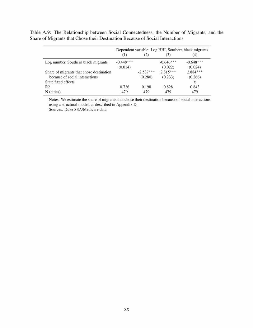
Table A.9: The Relationship between Social Connectedness, the Number of Migrants, and theShare of Migrants that Chose their Destination Because of Social Interactions
Dependent variable: Log HHI, Southern black migrants(1) (2) (3) (4)
Log number, Southern black migrants -0.448*** -0.646*** -0.648***(0.014) (0.022) (0.024)
Share of migrants that chose destination -2.537*** 2.815*** 2.884***because of social interactions (0.280) (0.233) (0.266)
State fixed effects xR2 0.726 0.198 0.828 0.843N (cities) 479 479 479 479
Notes: We estimate the share of migrants that chose their destination because of social interactionsusing a structural model, as described in Appendix D.Sources: Duke SSA/Medicare data
xx
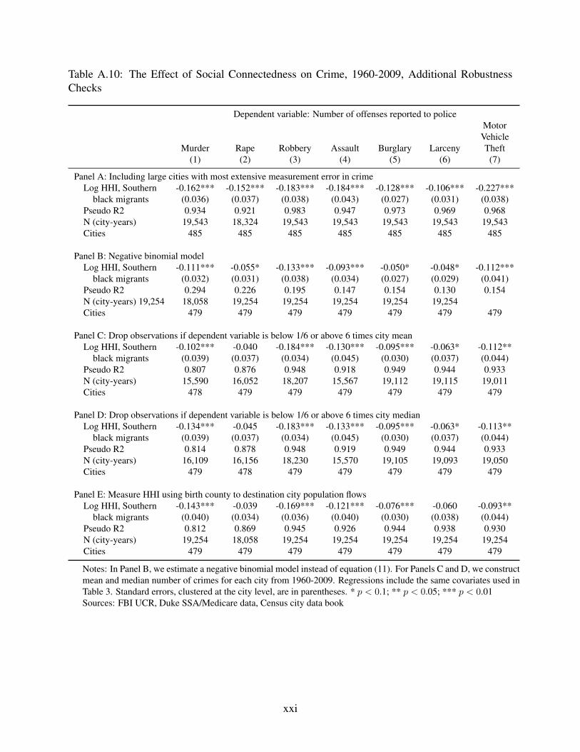
Table A.10: The Effect of Social Connectedness on Crime, 1960-2009, Additional RobustnessChecks
Dependent variable: Number of offenses reported to policeMotorVehicle
Murder Rape Robbery Assault Burglary Larceny Theft(1) (2) (3) (4) (5) (6) (7)
Panel A: Including large cities with most extensive measurement error in crimeLog HHI, Southern -0.162*** -0.152*** -0.183*** -0.184*** -0.128*** -0.106*** -0.227***
black migrants (0.036) (0.037) (0.038) (0.043) (0.027) (0.031) (0.038)Pseudo R2 0.934 0.921 0.983 0.947 0.973 0.969 0.968N (city-years) 19,543 18,324 19,543 19,543 19,543 19,543 19,543Cities 485 485 485 485 485 485 485
Panel B: Negative binomial modelLog HHI, Southern -0.111*** -0.055* -0.133*** -0.093*** -0.050* -0.048* -0.112***
black migrants (0.032) (0.031) (0.038) (0.034) (0.027) (0.029) (0.041)Pseudo R2 0.294 0.226 0.195 0.147 0.154 0.130 0.154N (city-years) 19,254 18,058 19,254 19,254 19,254 19,254 19,254Cities 479 479 479 479 479 479 479
Panel C: Drop observations if dependent variable is below 1/6 or above 6 times city meanLog HHI, Southern -0.102*** -0.040 -0.184*** -0.130*** -0.095*** -0.063* -0.112**
black migrants (0.039) (0.037) (0.034) (0.045) (0.030) (0.037) (0.044)Pseudo R2 0.807 0.876 0.948 0.918 0.949 0.944 0.933N (city-years) 15,590 16,052 18,207 15,567 19,112 19,115 19,011Cities 478 479 479 479 479 479 479
Panel D: Drop observations if dependent variable is below 1/6 or above 6 times city medianLog HHI, Southern -0.134*** -0.045 -0.183*** -0.133*** -0.095*** -0.063* -0.113**
black migrants (0.039) (0.037) (0.034) (0.045) (0.030) (0.037) (0.044)Pseudo R2 0.814 0.878 0.948 0.919 0.949 0.944 0.933N (city-years) 16,109 16,156 18,230 15,570 19,105 19,093 19,050Cities 479 478 479 479 479 479 479
Panel E: Measure HHI using birth county to destination city population flowsLog HHI, Southern -0.143*** -0.039 -0.169*** -0.121*** -0.076*** -0.060 -0.093**
black migrants (0.040) (0.034) (0.036) (0.040) (0.030) (0.038) (0.044)Pseudo R2 0.812 0.869 0.945 0.926 0.944 0.938 0.930N (city-years) 19,254 18,058 19,254 19,254 19,254 19,254 19,254Cities 479 479 479 479 479 479 479
Notes: In Panel B, we estimate a negative binomial model instead of equation (11). For Panels C and D, we constructmean and median number of crimes for each city from 1960-2009. Regressions include the same covariates used inTable 3. Standard errors, clustered at the city level, are in parentheses. * p < 0.1; ** p < 0.05; *** p < 0.01Sources: FBI UCR, Duke SSA/Medicare data, Census city data book
xxi

Table A.11: The Effect of Social Connectedness on Crime, 2000-2009, by Predicted Crimes
Dependent variable: Number of offenses reported to policeMotorVehicle
Murder Rape Robbery Assault Burglary Larceny Theft(1) (2) (3) (4) (5) (6) (7)
All Cities -0.077 0.086 -0.055 -0.161*** -0.022 -0.038 -0.045(0.078) (0.063) (0.051) (0.052) (0.043) (0.041) (0.057)
Below Median Predicted Crimes -0.021 0.124 -0.065 0.042 0.043 -0.013 0.195**(0.095) (0.084) (0.071) (0.074) (0.066) (0.055) (0.079)
Above Median Predicted Crimes -0.089 0.095 -0.068 -0.209*** -0.046 -0.046 -0.049(0.083) (0.077) (0.060) (0.064) (0.050) (0.046) (0.070)
Notes: Table displays estimates of equation (11). Regressions include the same covariates used in Table 3. Togenerate the predicted number of crimes for each city, we estimate equation (11) using data from 1995-1999,replacing state-year fixed effects with state-specific linear time trends. We then predict the number of crimeswith these coefficients and covariates from 2000-2009, using the average value of log HHI and log number ofmigrants for all cities when generating the prediction. We divide the sample on the basis of average number ofpredicted crimes per year from 2000-2009, and we estimate regressions using data from 2000-2009. Standarderrors, clustered at the city level, are in parentheses. * p < 0.1; ** p < 0.05; *** p < 0.01Sources: FBI UCR, Duke SSA/Medicare data, Census city data book
xxii

Figure A.1: Share of African Americans Born in the South Living Outside the South in Their 40s
0.0
5.1
.15
.2.2
5.3
.35
.4S
hare
livi
ng o
utsi
de o
f Sou
th
1890 1900 1910 1920 1930 1940 1950 1960Year of birth
Notes: Sample contains African Americans from the eleven former Confederate states. For individuals born from1891-1900, we measure their location using the 1900 Census. For individuals born from 1901-1910, we use the 1910Census, and so forth. The shaded circles correspond to individuals born from 1916-1936, who comprise our samplefrom the Duke SSA/Medicare data.Source: IPUMS Census data, 1940-2000
xxiii
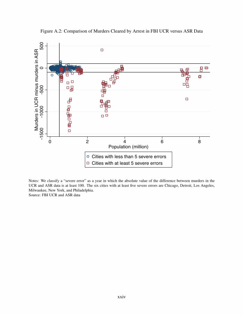
Figure A.2: Comparison of Murders Cleared by Arrest in FBI UCR versus ASR Data
-150
0-1
000
-500
050
0M
urde
rs in
UC
R m
inus
mur
ders
in A
SR
0 2 4 6 8Population (million)
Cities with less than 5 severe errorsCities with at least 5 severe errors
Notes: We classify a “severe error” as a year in which the absolute value of the difference between murders in theUCR and ASR data is at least 100. The six cities with at least five severe errors are Chicago, Detroit, Los Angeles,Milwaukee, New York, and Philadelphia.Source: FBI UCR and ASR data
xxiv

Figure A.3: The Relationship Between the Number of Murders Cleared by Arrest in UCR and ASR Data, 1960-20090
200
400
600
800
1000
1200
1960 1970 1980 1990 2000 2010Year
Murders, UCR Murders, ASR
(a) Chicago
050
010
0015
0020
00
1960 1970 1980 1990 2000 2010Year
Murders, UCR Murders, ASR
(b) Detroit
025
050
075
010
0012
5015
00
1960 1970 1980 1990 2000 2010Year
Murders, UCR Murders, ASR
(c) Los Angeles
010
020
030
040
050
0
1960 1970 1980 1990 2000 2010Year
Murders, UCR Murders, ASR
(d) Milwaukee
025
050
075
010
0012
5015
00
1960 1970 1980 1990 2000 2010Year
Murders, UCR Murders, ASR
(e) New York
010
020
030
040
050
0
1960 1970 1980 1990 2000 2010Year
Murders, UCR Murders, ASR
(f) Philadelphia
Notes: ASR data are first available in 1980. The cities in Appendix Figure A.3 are those for which the absolute value of the difference in murders between UCRand ASR data is at least 100 for at least five years.Source: FBI UCR and ASR data
xxv

Figure A.4: The Relationship between Social Connectedness and the Number of Southern BlackMigrants
Linear fit: -0.44 ( 0.01), R2 = 0.72
-6-5
-4-3
-2Lo
g H
HI,
Sou
ther
n bl
ack
mig
rant
s
3 4 5 6 7 8 9 10Log number, Southern black migrants
25,000-149,999 150,000-499,999 500,000+1980 Population
Notes: Figure contains 412 cities.Source: Duke SSA/Medicare data
xxvi
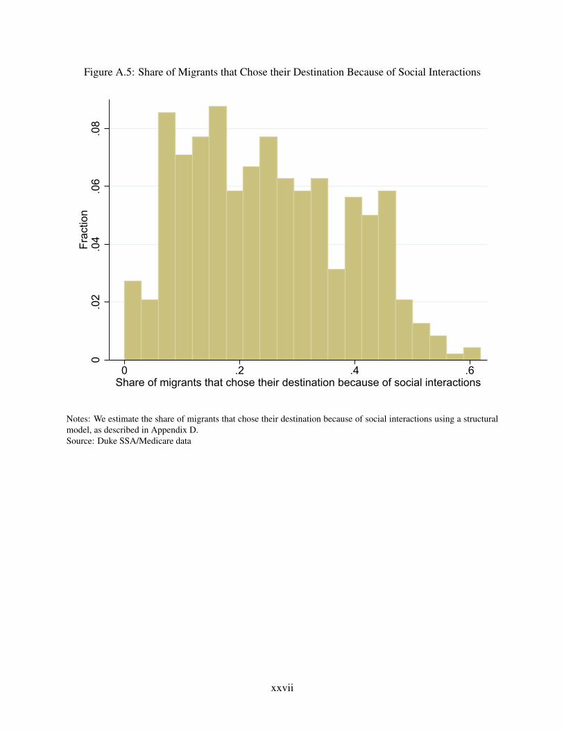
Figure A.5: Share of Migrants that Chose their Destination Because of Social Interactions
0.0
2.0
4.0
6.0
8Fr
actio
n
0 .2 .4 .6Share of migrants that chose their destination because of social interactions
Notes: We estimate the share of migrants that chose their destination because of social interactions using a structuralmodel, as described in Appendix D.Source: Duke SSA/Medicare data
xxvii
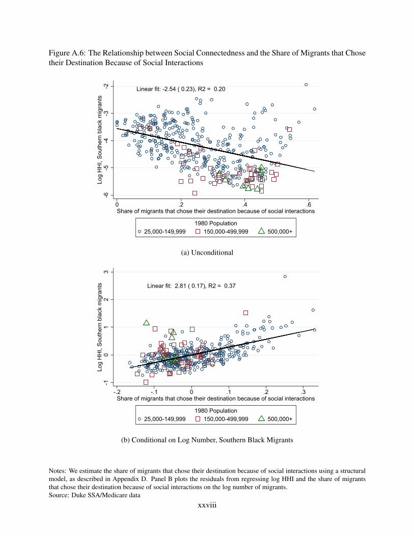
Figure A.6: The Relationship between Social Connectedness and the Share of Migrants that Chosetheir Destination Because of Social Interactions
Linear fit: -2.54 ( 0.23), R2 = 0.20
-6-5
-4-3
-2Lo
g H
HI,
Sou
ther
n bl
ack
mig
rant
s
0 .2 .4 .6Share of migrants that chose their destination because of social interactions
25,000-149,999 150,000-499,999 500,000+1980 Population
(a) Unconditional
Linear fit: 2.81 ( 0.17), R2 = 0.37
-10
12
3Lo
g H
HI,
Sou
ther
n bl
ack
mig
rant
s
-.2 -.1 0 .1 .2 .3Share of migrants that chose their destination because of social interactions
25,000-149,999 150,000-499,999 500,000+1980 Population
(b) Conditional on Log Number, Southern Black Migrants
Notes: We estimate the share of migrants that chose their destination because of social interactions using a structuralmodel, as described in Appendix D. Panel B plots the residuals from regressing log HHI and the share of migrantsthat chose their destination because of social interactions on the log number of migrants.Source: Duke SSA/Medicare data
xxviii