This paper presents preliminary findings and is being distributed to economists

and other interested readers solely to stimulate discussion and elicit comments.

The views expressed in this paper are those of the authors and are not necessarily

reflective of views at the Federal Reserve Bank of New York or the Federal

Reserve System. Any errors or omissions are the responsibility of the authors.

Federal Reserve Bank of New York

Staff Reports

The FRBNY DSGE Model

Marco Del Negro

Stefano Eusepi

Marc Giannoni

Argia Sbordone

Andrea Tambalotti

Matthew Cocci

Raiden Hasegawa

M. Henry Linder

Staff Report No. 647

October 2013

The FRBNY DSGE Model

Marco Del Negro, Stefano Eusepi, Marc Giannoni, Argia Sbordone, Andrea Tambalotti, Matthew

Cocci, Raiden Hasegawa, and M. Henry Linder

Federal Reserve Bank of New York Staff Reports, no. 647

October 2013

JEL classification: C53, C54, E52

Abstract

The goal of this paper is to present the dynamic stochastic general equilibrium (DSGE) model

developed and used at the Federal Reserve Bank of New York. The paper describes how the

model works, how it is estimated, how it rationalizes past history, including the Great Recession,

and how it is used for forecasting and policy analysis.

Key words: DSGE models

_________________

Del Negro, Eusepi, Giannoni, Sbordone, Tambalotti, Cocci, Hasegawa, Linder: Federal Reserve

Bank of New York (e-mail: marco.delnegro@ny.frb.org, stefano.eusepi@ny.frb.org,

marc.giannoni@ny.frb.org, argia.sbordone@ny.frb.org, andrea.tambalotti@ny.frb.org,

matthew.cocci@ny.frb.org, raiden.hasegawa@ny.frb.org, m.henry.linder@ny.frb.org). Address

correspondence to the Research Department, Federal Reserve Bank of New York, 33 Liberty

Street, New York, NY 10045. The authors are very grateful to the many talented research

assistants who have worked on the model over the years, in particular, Jenny Chan, Kailin Clarke,

Dan Greenwald, Dan Herbst, and Christina Patterson. The views expressed in this paper are those

of the authors and do not necessarily reflect the position of the Federal Reserve Bank of New

York or the Federal Reserve System.

1

Contents

1 Introduction 2

2 The DSGE Model 3

2.1 General Features of the Model . . . . . . . . . . . . . . . . . . . . . . . . . . 4

2.2 The Model Microfoundations . . . . . . . . . . . . . . . . . . . . . . . . . . . 6

2.3 The Model in Log-linear Form . . . . . . . . . . . . . . . . . . . . . . . . . . 12

2.4 The Exogenous Processes . . . . . . . . . . . . . . . . . . . . . . . . . . . . . 16

3 Estimation and Data 16

4 Priors and Posterior Estimates for the DSGE Model Parameters 19

5 The Transmission Mechanism and the Variance Decomposition 20

5.1 Policy Shocks: Anticipated and Unanticipated . . . . . . . . . . . . . . . . . 23

6 Developing a Narrative: from the Great Recession to a Sluggish Recovery 25

7 The Forecast Distributions 29

8 An Assessment of the Model’s Real-Time Forecasts, 2010-2012 29

9 Conclusion 31

Tables 35

Figures 37

A Measurement Equations 54

2

1 Introduction

The goal of this paper is to present the FRBNY DSGE model, that is, the dynamic stochastic

general equilibrium (DSGE) model developed and used at the Federal Reserve Bank of New

York. The paper describes how the model works, how it is estimated, how it rationalizes past

history including the Great Recession, and how it is used for forecasting and policy analysis.

Models, unless they are very simple, are often perceived as black boxes. This problem

is particularly prevalent for DSGE models which are necessarily complicated to capture

the fundamentally dynamic relationships in the economy as well as the general equilibrium

forces that drive most macroeconomic variables. In addition, the Bayesian techniques used

for the estimation of these models may seem mysterious. We are providing here a fairly

detailed description of the FRBNY DSGE model. Such a description is necessarily somewhat

technical. However, to make sure that most readers understand the key features of the

model, we complement the model description with more intuitive discussions of the model’s

ingredients and implications.

The FRBNY DSGE model is a medium scale, one-sector dynamic stochastic general

equilibrium model. It builds on the neo-classical growth model by adding nominal wage and

price rigidities, variable capital utilization, costs of adjusting investment, habit formation in

consumption, and credit frictions. The core of the model is based on the work of Smets and

Wouters (2007), and Christiano et al. (2005), and includes credit frictions as in the financial

accelerator model developed by Bernanke et al. (1999). The actual implementation of the

credit frictions follows closely Christiano et al. (2009).

The model is perturbed by a set of exogenous shocks, which are the fundamental sources

of macroeconomic fluctuations. These shocks are identified by matching the model dynamics

with the following quarterly data series: real GDP growth, core PCE inflation, the labor

share, aggregate hours worked, the effective federal funds rate (FFR), and the spread between

Baa corporate bonds and 10-year Treasury yields. In addition, we use data on federal funds

rate expectations as measured by OIS rates, starting in 2008Q4, i.e., when the policy rate

hit the zero lower bound. The parameters of the model are estimated on data from 1984Q1

to 2013Q1 using Bayesian methods as presented for instance in An and Schorfheide (2007)

and Del Negro and Schorfheide (2010).

DSGE models have a number of key advantages over alternative models, as discussed

3

e.g., in Sbordone et al. (2010). First, by being built on microeconomic foundations, these

models make clear how economic agents’ current decisions depend on their expectations

about uncertain future outcomes. Second, the general equilibrium feature of these models

imply an important interaction between policy actions and households or firms’ behavior.

Moreover, the clear specification of the stochastic shocks allows one to identify the source of

economic fluctuations.

The fact that DSGE modelers can readily take advantage of progress in academic research

by incorporating new features and new inference procedures into their models is arguably

another key advantage of DSGE models relative to alternative approaches. This also means

however that DSGE models evolve over time to keep up with advances in research, and the

FRBNY DSGE model is no exception. What we present here is therefore just a snapshot of

the model at this point in time. In spite of the fact that this model will continue to evolve

over time, it seemed worthwhile to document where we currently stand.

The remainder of the paper is as follows. Section 2 describes the model, first at a

general level and then more in detail. Section 3 elaborates on the estimation procedure,

including the use of anticipated monetary policy shocks to model forward guidance. Section

4 discusses the prior information on the model’s parameters, which is based in large part

based on the calibration literature, and their posterior distribution. Section 5 illustrates the

estimated model’s transmission mechanism, with particular emphasis on the propagation

of anticipated policy shocks. Section 6 provides the model’s interpretation of the Great

Recession. Section 7 shows the model’s forecasts as of June 2013, and elaborates on how this

structural model can be used to interpret the outlook. The model’s forecasts are distinct

from the FRBNY staff forecasts. Section 8 provides an assessment of the model’s real time

forecasts over the past three years. Finally, section 9 concludes.

2 The DSGE Model

This section is structured as follows. We first describe the general features of the model by

introducing its main economic units and briefly discussing their role, the various frictions that

affect their interrelationships, and the source of exogenous disturbances. Next we detail the

microfoundations of the model — the form of preferences, technology, and constraints and

the shock processes — and present the optimization problem of each set of agents. Solving

4

these optimization problems result in optimal decision rules that describe the behavior of

each set of agents. Rather than attempting to solve the full set of model equations, we

proceed by performing a log-linear approximation to all equilibrium conditions. We describe

at the end of the section the set of log-linearized equilibrium conditions, which are needed

to reproduce our results.

2.1 General Features of the Model

The economic units in the model are households, firms, banks, entrepreneurs, and the gov-

ernment. Figure 1 illustrates the interactions among these units, the model frictions and the

shocks that affect the economy’s dynamics.

Households supply labor services to firms. The utility they derive from leisure is subject

to a random disturbance, which we call “labor supply” shock, since it captures exogenous

movements in labor supply due to factors such as demographics and labor market imperfec-

tions (this shock is sometimes also referred to as a “leisure” shock). Frictions in the labor

market take the form of nominal wage rigidities. These frictions imply that various shocks

affect hours worked. Households also choose how much to consume and to save. Their sav-

ings take the form of deposits into banks and purchases of government bonds. Households’

preferences for consumption incorporate habit persistence, a characteristic that affects their

consumption smoothing decisions.

Monopolistically competitive firms produce intermediate goods, which a competitive firm

aggregates into a single final good that is used for both consumption and investment. The

production function of intermediate producers is subject to “total factor productivity” (TFP)

shocks. Frictions in the intermediate goods markets take the form of nominal price rigidities.

Together with wage rigidities, this friction allows demand shocks to be a source of business

cycle fluctuations, as countercyclical mark-ups induce firms to produce less when demand

is low. Firms’ optimal price setting implies that inflation evolves in the model according

to a standard, forward-looking New Keynesian Phillips curve, which determines inflation

as a function of marginal costs, expected future inflation, and “mark-up” shocks. Mark-

up shocks capture exogenous changes in the degree of competitiveness in the intermediate

goods market. In practice, these shocks capture also unmodeled inflationary pressures, such

as those arising from fluctuations in commodity prices.

5

Financial intermediation involves two actors, banks and entrepreneurs, whose interac-

tion captures imperfections in financial markets. These agents should not be interpreted

in a literal sense, but rather as a device for modeling credit frictions. Banks collect de-

posits from households and lend to entrepreneurs. Entrepreneurs use their own wealth and

loans from the banks to acquire capital, which they rent to intermediate good producers.

Entrepreneurs are subject to idiosyncratic disturbances that affect their ability to manage

capital. Consequently, their revenues may not be high enough to repay their borrowing, in

which case they default. Banks protect themselves against default risk by pooling loans to

all entrepreneurs and charging them a spread over the deposit rate. The spread varies both

endogenously, as a function of the entrepreneurs’ leverage, as well as exogenously on the

basis of entrepreneurs’ riskiness. In particular, mean-preserving changes in the volatility of

entrepreneurs’ idiosyncratic shocks lead to variations in the spread, to compensate banks for

expected losses from defaults. We refer to these exogenous movements in risk as “spread”

shocks. Spread shocks, which capture various disturbances to the financial intermediation

process, affect entrepreneurs’ borrowing costs, altering their demand for capital, and hence

investment.

Capital producers transform general output into capital goods, which they sell to the

entrepreneurs. The production of new capital is subject to convex adjustment costs, making

the production of capital goods more costly in periods of rapid investment growth. It is also

subject to exogenous changes in the “marginal efficiency of investment” (MEI). These MEI

shocks capture exogenous movements in the productivity of new investments in generating

new capital. A positive MEI shock implies that fewer resources are needed to build new

capital, leading to higher real activity and inflation, with an effect that persists over time.

Such MEI shocks reflect both changes in the relative price of investment versus consumption

goods as well as financial market imperfections that are not reflected in movements of the

spread (Justiniano et al. (2010)).

Finally, the government sector comprises a monetary authority that sets short-term in-

terest rates according to a Taylor-type rule and a fiscal authority that sets public spending

and collects lump-sum taxes. Exogenous changes in government spending are called “gov-

ernment” shocks; more generally, these shocks capture exogenous movements in aggregate

demand.

6

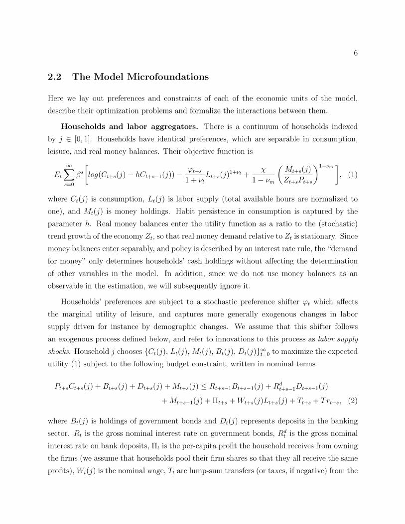
2.2 The Model Microfoundations

Here we lay out preferences and constraints of each of the economic units of the model,

describe their optimization problems and formalize the interactions between them.

Households and labor aggregators. There is a continuum of households indexed

by j ∈ [0, 1]. Households have identical preferences, which are separable in consumption,

leisure, and real money balances. Their objective function is

Et

∞∑s=0

βs[log(Ct+s(j)− hCt+s−1(j))− ϕt+s

1 + νlLt+s(j)

1+νl +χ

1− νm

(Mt+s(j)

Zt+sPt+s

)1−νm ], (1)

where Ct(j) is consumption, Lt(j) is labor supply (total available hours are normalized to

one), and Mt(j) is money holdings. Habit persistence in consumption is captured by the

parameter h. Real money balances enter the utility function as a ratio to the (stochastic)

trend growth of the economy Zt, so that real money demand relative to Zt is stationary. Since

money balances enter separably, and policy is described by an interest rate rule, the “demand

for money” only determines households’ cash holdings without affecting the determination

of other variables in the model. In addition, since we do not use money balances as an

observable in the estimation, we will subsequently ignore it.

Households’ preferences are subject to a stochastic preference shifter ϕt which affects

the marginal utility of leisure, and captures more generally exogenous changes in labor

supply driven for instance by demographic changes. We assume that this shifter follows

an exogenous process defined below, and refer to innovations to this process as labor supply

shocks. Household j chooses {Ct(j), Lt(j), Mt(j), Bt(j), Dt(j)}∞t=0 to maximize the expected

utility (1) subject to the following budget constraint, written in nominal terms

Pt+sCt+s(j) +Bt+s(j) +Dt+s(j) +Mt+s(j) ≤ Rt+s−1Bt+s−1(j) +Rdt+s−1Dt+s−1(j)

+Mt+s−1(j) + Πt+s +Wt+s(j)Lt+s(j) + Tt+s + Trt+s, (2)

where Bt(j) is holdings of government bonds and Dt(j) represents deposits in the banking

sector. Rt is the gross nominal interest rate on government bonds, Rdt is the gross nominal

interest rate on bank deposits, Πt is the per-capita profit the household receives from owning

the firms (we assume that households pool their firm shares so that they all receive the same

profits), Wt(j) is the nominal wage, Tt are lump-sum transfers (or taxes, if negative) from the

7

government, and Trt are net per-capita lump-sum transfers from the entrepreneurs (discussed

later).

We assume that households have access to a full menu of state-contingent securities,

although to simplify the notation we do not explicitly add these securities to the budget

constraint. Because of this assumption, all households choose the same consumption, money

demand, bond holdings and bank deposits. The choice of hours worked can however differ

across households, since they will face different wages in equilibrium.

The labor input supplied to the intermediate goods producers, Lt, is a composite of all

the labor services supplied by each household j. We assume the existence of competitive

labor aggregators (or “employment agencies”) which combine individual households’ labor

into an aggregate Lt, sold to the intermediate goods producers

Lt =

[ ∫ 1

0

Lt(j)1

1+λw dj

]1+λw

. (3)

The parameter λw ∈ (0,∞) affects the elasticity of substitution between differentiated labor

services.

The first-order condition of the employment agencies’ problem leads to the following

labor demand schedule Lt(j) for labor services of household j:

Lt(j) =

(Wt(j)

Wt

)− 1+λwλw

Lt, (4)

where Wt(j) is the wage paid to Lt(j) and Wt is the aggregate wage, defined as

Wt =

[ ∫ 1

0

Wt(j)1λw dj

]λw. (5)

Every household has market power and chooses its nominal wage subject to the demand

constraint (4). However, we assume nominal wage rigidity a la Calvo (1983): in every period,

each household has a probability 1 − ζw of choosing its wage freely. The households that

cannot do so simply increase Wt(j) by the steady-state growth rate of aggregate wages (equal

to steady state inflation π∗ times the growth rate of the economy eγ). Instead, households

that can optimize at time t choose a wage Wt(j) to maximize:

Et

∞∑s=0

(ζwβ)s[− ϕt+s

1 + νlLt+s(j)

1+νl

], (6)

8

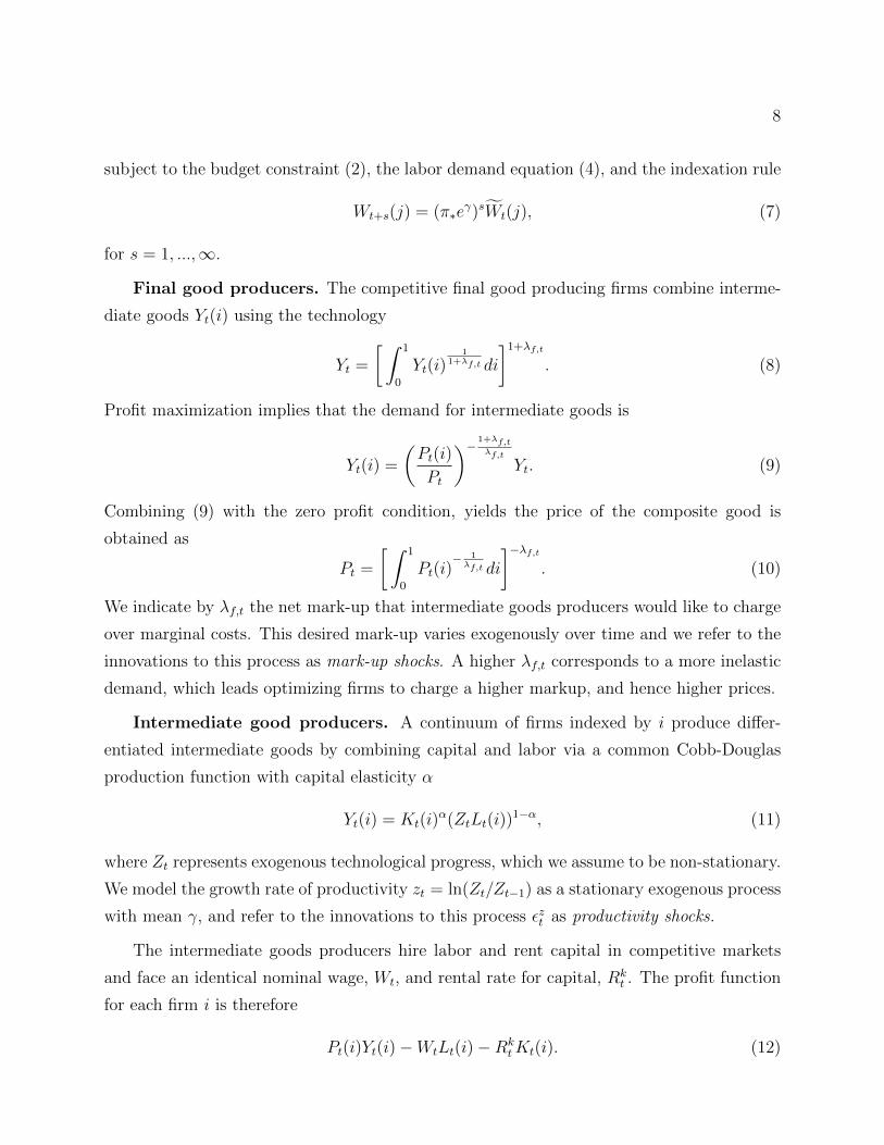
subject to the budget constraint (2), the labor demand equation (4), and the indexation rule

Wt+s(j) = (π∗eγ)sWt(j), (7)

for s = 1, ...,∞.

Final good producers. The competitive final good producing firms combine interme-

diate goods Yt(i) using the technology

Yt =

[ ∫ 1

0

Yt(i)1

1+λf,t di

]1+λf,t

. (8)

Profit maximization implies that the demand for intermediate goods is

Yt(i) =

(Pt(i)

Pt

)− 1+λf,tλf,t

Yt. (9)

Combining (9) with the zero profit condition, yields the price of the composite good is

obtained as

Pt =

[ ∫ 1

0

Pt(i)− 1λf,t di

]−λf,t. (10)

We indicate by λf,t the net mark-up that intermediate goods producers would like to charge

over marginal costs. This desired mark-up varies exogenously over time and we refer to the

innovations to this process as mark-up shocks. A higher λf,t corresponds to a more inelastic

demand, which leads optimizing firms to charge a higher markup, and hence higher prices.

Intermediate good producers. A continuum of firms indexed by i produce differ-

entiated intermediate goods by combining capital and labor via a common Cobb-Douglas

production function with capital elasticity α

Yt(i) = Kt(i)α(ZtLt(i))

1−α, (11)

where Zt represents exogenous technological progress, which we assume to be non-stationary.

We model the growth rate of productivity zt = ln(Zt/Zt−1) as a stationary exogenous process

with mean γ, and refer to the innovations to this process εzt as productivity shocks.

The intermediate goods producers hire labor and rent capital in competitive markets

and face an identical nominal wage, Wt, and rental rate for capital, Rkt . The profit function

for each firm i is therefore

Pt(i)Yt(i)−WtLt(i)−RktKt(i). (12)

9

Following Calvo (1983), we assume that in every period a fraction (1− ζp) of the inter-

mediate goods producers optimize their prices and the remainder ζp adjusts prices to steady

state inflation π∗. The firms that are able to optimize choose prices Pt(i) to maximize the

expected discounted sum of future profits:

Ξpt (Pt(i)−MCt)Yt(i) + IEt

∞∑s=1

ζspβsΞp

t+s(Pt(i)π∗s −MCt+s)Yt+s(i)

subject to

Yt+s(i) =

(Pt(i)π∗

s

Pt+s

)−(1+ 1λf,t+s

)

Yt+s.

where πt ≡ PtPt−1

, MCt is firms’ nominal marginal cost, and βsΞpt+s is a discount factor (Ξp

t is

the Lagrange multiplier associated with the households’ nominal budget constraint).

Capital producers. Capital producers are competitive firms that purchase an amount

of capital x from entrepreneurs at the beginning of the period. During the period, they buy

an amount I of general output from the final goods producers, and transform it into new

capital via the technology:

x′ = x+ µt

(1− S

(ItIt−1

))It, (13)

so that x′ is the new stock of capital, which they sell back to entrepreneurs at the end of the

same period. It is investment spending and S(·) is the cost of adjusting investment, with

S ′(·) > 0, S ′′(·) > 0. The exogenous process µt affects the efficiency by which a foregone

unit of consumption contributes to capital accumulation, and its innovations are labeled

“marginal efficiency of investment” (MEI) shocks. Capital producers choose investment to

maximize their profits, expressed in terms of consumption goods,

Πkt =

Qkt

Pt(x′ − x)− It, (14)

where Qkt is the price of capital.

Entrepreneurs and Banks. There is a continuum of entrepreneurs indexed by e. Each

entrepreneur buys installed capital Kt−1(e) from the capital producers at the end of period

t− 1 using her own net worth Nt−1(e) and a loan Bdt−1(e) from the banking sector, so that:

Qkt−1Kt−1(e) = Bd

t−1(e) +Nt−1(e), (15)

10

where net worth is expressed in nominal terms. In the next period she rents capital to

intermediate good producing firms, earning a rental rate Rkt per unit of effective capital. In

period t an idiosyncratic shock ωt(e), i.i.d. across entrepreneurs and over time, may increase

or shrink entrepreneurs’ capital. We denote by Ft−1(ω) the cumulative distribution function

of ω at time t, which is assumed to be known at time t− 1. After observing the shock, the

entrepreneur chooses a level of capital utilization ut(e) by paying a cost in terms of general

output equal to a(ut(e)) per-unit-of-capital. At the end of period t the entrepreneur sells

the depreciated capital to the capital producers.

Entrepreneurs’ revenues (net of utilization cost) in period t are therefore:

ωt(e)Rkt (e)Q

kt−1Kt−1(e) (16)

where

Rkt (e) =

Rkt ut(e) + (1− δ)Qk

t − Pta(ut(e))

Qkt−1

(17)

is the gross nominal return to capital for entrepreneurs, and δ is the capital depreciation

rate. Since the choice of the utilization rate, given by Rkt /Pt = a′(ut(e)), is independent of

the amount of capital purchased and of the ωt shock, we drop the index e from the return

Rkt in what follows.

The debt contract undertaken by the entrepreneur in period t− 1 consists of the triplet

(Bdt−1(e), Rc

t(e), ωt(e)) where Bdt−1(e) is the entrepreneur’s debt, Rc

t(e) represents the con-

tractual interest rate, and ωt(e) is a ‘bankruptcy’ threshold: for realizations ωt(e) < ωt(e)

the entrepreneur defaults on her debt. The threshold is therefore defined by the equation:

ωt(e)RktQ

kt−1Kt−1(e) = Rc

t(e)Bdt−1(e). (18)

The model features a representative bank that collects deposits from households, on

which it pays an interest rate Rdt , and lends to entrepreneurs. Loan contracts are subject to

costly state verification: verification costs are a fraction µe of the amount the bank extracts

from the entrepreneur in case of bankruptcy. The bank’s zero profit condition implies that:

[1− Ft−1(ωt(e))]Rct(e)B

dt−1(e) + (1− µe)

∫ ωt(e)

0

ωdFt−1(ω)RktQ

kt−1Kt−1(e) = Rd

t−1Bdt−1(e)

(19)

11

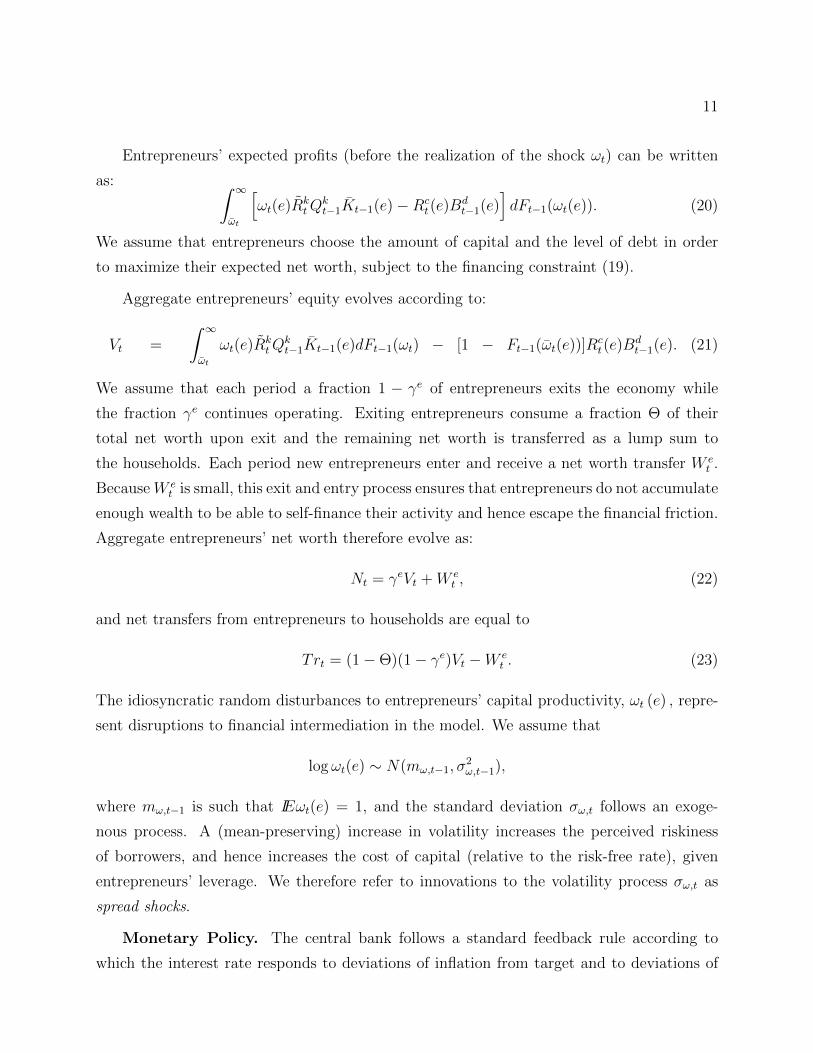
Entrepreneurs’ expected profits (before the realization of the shock ωt) can be written

as: ∫ ∞ωt

[ωt(e)R

ktQ

kt−1Kt−1(e)−Rc

t(e)Bdt−1(e)

]dFt−1(ωt(e)). (20)

We assume that entrepreneurs choose the amount of capital and the level of debt in order

to maximize their expected net worth, subject to the financing constraint (19).

Aggregate entrepreneurs’ equity evolves according to:

Vt =

∫ ∞ωt

ωt(e)RktQ

kt−1Kt−1(e)dFt−1(ωt) − [1 − Ft−1(ωt(e))]R

ct(e)B

dt−1(e). (21)

We assume that each period a fraction 1 − γe of entrepreneurs exits the economy while

the fraction γe continues operating. Exiting entrepreneurs consume a fraction Θ of their

total net worth upon exit and the remaining net worth is transferred as a lump sum to

the households. Each period new entrepreneurs enter and receive a net worth transfer W et .

BecauseW et is small, this exit and entry process ensures that entrepreneurs do not accumulate

enough wealth to be able to self-finance their activity and hence escape the financial friction.

Aggregate entrepreneurs’ net worth therefore evolve as:

Nt = γeVt +W et , (22)

and net transfers from entrepreneurs to households are equal to

Trt = (1−Θ)(1− γe)Vt −W et . (23)

The idiosyncratic random disturbances to entrepreneurs’ capital productivity, ωt (e) , repre-

sent disruptions to financial intermediation in the model. We assume that

logωt(e) ∼ N(mω,t−1, σ2ω,t−1),

where mω,t−1 is such that IEωt(e) = 1, and the standard deviation σω,t follows an exoge-

nous process. A (mean-preserving) increase in volatility increases the perceived riskiness

of borrowers, and hence increases the cost of capital (relative to the risk-free rate), given

entrepreneurs’ leverage. We therefore refer to innovations to the volatility process σω,t as

spread shocks.

Monetary Policy. The central bank follows a standard feedback rule according to

which the interest rate responds to deviations of inflation from target and to deviations of

12

output growth from its steady state:

Rt

R=

(Rt−1

R

)ρR[(Π3j=0

πt−jπ∗

)ψπ( YtYt−4

e−4γ

)ψY ]1−ρReεRt ΠK

k=1eεRk,t−k . (24)

In (24) R is the steady state (gross) nominal interest rate, π∗ is the inflation target, Π3j=0πt−j

is the 4-quarter gross inflation rate, YtYt−4

is the 4-quarter gross growth rate of output, and e4γ

is the gross annualized steady-state growth rate of the economy; ψπ and ψy are the central

bank’s reaction coefficients, and ρR captures persistence in the reaction function. εR,t is a

monetary policy shock, where εRt ∼ N(0, σ2r), i.i.d., and εRk,t−k are anticipated policy shocks.

The latter are policy shocks which are known to agents at time t−k, but affect the policy rule

k periods later, that is, at time t. We assume that εRk,t−k ∼ N(0, σ2k,r), i.i.d. The purpose of

introducing anticipated policy shocks is to constrain the path of the interest rate, which may

be needed to enforce the zero lower bound constraint and/or to implement policymakers’

‘forward guidance’ on the future path of the interest rate.

Fiscal Policy. Fiscal policy is fully Ricardian so that the timing of taxes does not affect

the equilibrium. Public spending is determined exogenously as a time-varying fraction of

aggregate output

Gt = (1− 1/gt)Yt, (25)

where government spending gt follows an exogenous process, and we refer to the innovations

to this process, εgt , as demand shocks, with εgt ∼ N(0, σ2g), i.i.d..

Market clearing. Combining the government’s and households’ budget constraints

with the zero profit condition of final goods producers and employment agencies yields the

aggregate resource constraint

Ct + It + a(ut)Kt−1 =1

gtYt. (26)

The optimization conditions of the model result in dynamic relationships among macroe-

conomic variables. Together with market clearing conditions, they completely characterize

the equilibrium behavior of the model economy.

2.3 The Model in Log-linear Form

The model has a source of non-stationarity in the process for technology Zt, which has a

unit root. Hence consumption, investment, capital, real wages and output inherit stochastic

13

growth. To solve the model we first rewrite its equilibrium conditions in terms of stationary

variables and solve for the non-stochastic steady state of the transformed model. Then we

take a log-linear approximation of the transformed model around its steady state. This

approximation generates a set of log-linear equations, which we solve to obtain the model’s

state-space representation, using the method of Sims (2002). We then use the state-space

representation in the estimation procedure.

Below we list the log-linear equations of the model. We follow the usual convention of

denoting log-deviations from steady state with hatted variables: for any stationary variable

xt, xt ≡ log(xt/x∗), where x∗ denotes its steady state value. The steady state itself is a

function of the model’s parameters. Equations describing the mapping between parameters

and steady state variables are available upon request.

The Consumption Euler Equation that characterizes the optimal allocation of consump-

tion over time is given by

ξt = Rt + IEt[ξt+1]− IEt[zt+1]− IEt[πt+1], (27)

where Rt is the gross nominal interest rate on government bonds, and ξt is the marginal

utility of consumption.

The Marginal Utility of Consumption ξt evolves according to

(eγ − hβ)(eγ − h)ξt = − (e2γ + βh2)ct + heγ ct−1 − heγ zt

+ βheγIEt[ct+1] + βheγIEt[zt+1],

where ct is consumption, eγ is the steady-state (gross) growth rate of the economy and h

captures habit persistence in consumption.

The Capital Stock follows

ˆkt = −(1− i∗k∗

)zt + (1− i∗k∗

)ˆkt−1 +i∗k∗µt +

i∗k∗ıt, (28)

where ˆkt is installed capital, zt is the growth rate of productivity, i∗ and k∗ are steady state

investment and the level of capital, respectively, and µt is the exogenous process that affects

the efficiency by which a foregone unit of consumption contributes to capital utilization.

The Effective Capital kt is in turn given by

kt = ut − zt + ˆkt−1, (29)

14

where ut is the level of capital utilization.

Capital Utilization is given by

rk∗ rkt = a′′ (u) ut, (30)

where rk∗ is the steady state rental rate of capital and the function a (u) captures the utiliza-

tion cost.

The Optimal Investment decision satisfies the Euler equation

it =1

1 + βIEt [ıt−1 − zt] +

β

1 + βIEt [ıt+1 + zt+1] +

1

(1 + β)S ′′e2γqkt +

1

(1 + β)S ′′e2γµt, (31)

where it is investment, S (.) is the cost of adjusting capital, with S ′ and S ′′ > 0, and qkt is

the price of capital.

The Realized Return on Capital is given by:

Rk

t − πt =rk∗

rk∗ + (1− δ)rkt +

(1− δ)rk∗ + (1− δ)

qkt − qkt−1, (32)

where δ is the rate of capital depreciation, πt is the inflation rate, whose evolution is described

below, rkt is the capital rental rate and qkt is the price of capital.

The Expected Excess Return on Capital (or ‘spread’)

IEt

[Rk

t+1 − Rt

]= ζsp,b

(qkt + kt − nt)+ σω,t (33)

can be expressed as a function of the entrepreneurs’ leverage (i.e., the ratio of the value

of capital to nominal net worth) and exogenous fluctuations in the volatility of the en-

trepreneurs’ idiosyncratic productivity, σω,t ≡ ζsp,σω σω,t. The parameter ζsp,b is the elasticity

of the spread with respect to leverage, and ζsp,σω is the elasticity of the spread with respect

to the volatility of the spread shock.

The Entrepreneurs’ Net Worth, nt, evolves according to

nt = ζn,Rk

(Rk

t − πt)− ζn,R

(Rt−1 − πt

)+ ζn,qK

(qkt−1 + kt−1

)+ ζn,nnt−1 − γe

v∗n∗zt −

ζn,σωζsp,σω

σω,t−1, (34)

15

where ζn,Rk , ζn,R, ζn,qK , ζn,n, and ζn,σω are the elasticities of net worth to the return on

capital, the nominal interest rate, the cost of capital, net worth itself and the volatility σω,

respectively, and γe is the fraction of entrepreneurs who survive each period.

The evolution of the Aggregate Nominal Wage is then given by

wt = wt−1 − πt +1− ζwζw

ˆwt, (35)

where ζw is the fraction of workers who cannot adjust their wages in a given period and ˆwt

is the optimal wage chosen by workers that can freely set it, or optimal reset wage.

The Optimal Reset Wage follows

(1 + νl1 + λwλw

) ˆwt + (1 + ζwβνl(1 + λwλw

))wt =

ζwβ(1 + νl1 + λwλw

)IEt[ ˆwt+1 + wt+1] + ϕt + (1− ζwβ)(νlLt − ξt)

+ ζwβ(1 + νl1 + λwλw

)IEt[πt+1 + zt+1],

where ϕt is a stochastic preference shifter affecting the marginal utility of leisure and λw

is the parameter that determines the elasticity of substitution between differentiated labor

services.

The optimal price-setting decision yields a Phillips Curve equation

πt = βIEt[πt+1] +(1− ζpβ)(1− ζp)

ζpmct +

1

ζpλf,t, (36)

where πt is inflation, mct is nominal marginal cost, β is the discount factor, and ζp is the

Calvo parameter, representing the fraction of firms that cannot adjust their prices each

period. λf,t is the following re-parametrization of the cost-push shock λf,t : λf,t = [(1 −ζpβ)(1− ζp)λf/(1 + λf )]λf,t, where λf is the steady state value of the markup shock.

The Marginal Cost (or labor share) satisfies

mct = (1− α)wt + αrkt , (37)

where α is the output elasticity to capital and rkt is the capital rental rate.

The Production Function is given by

yt = αkt + (1− α)Lt, (38)

16

where the Capital-Labor Ratio satisfies

kt = wt − rkt + Lt. (39)

The Resource Constraint is

yt = gt +c∗

c∗ + i∗ct +

i∗c∗ + i∗

ıt +rk∗k∗c∗ + i∗

ut, (40)

where yt is output and gt is government spending.

Finally, the Policy Rule is

Rt = ρRRt−1 + (1− ρR)

(ψπ

3∑j=0

πt−j + ψy

3∑j=0

(yt−j − yt−j−1 + zt−j)

)+ εRt +

K∑k=1

εRk,t−k, (41)

where∑3

j=0 πt−j is 4-quarter inflation expressed in deviation from the Central Bank’s ob-

jective π∗ (which corresponds to steady state inflation),∑3

j=0(yt−j − yt−j−1 + zt−j) is the

4-quarter growth rate of real GDP expressed in deviation from steady state growth, εRt is the

standard contemporaneous policy shock, and the terms εRk,t−k are anticipated policy shocks,

known to agents at time t− k.

2.4 The Exogenous Processes

The exogenous processes zt, ϕt, λf,t, µt, σω,t and gt are assumed to follow AR(1) processes

with autocorrelation parameters denoted by ρz, ρϕ, ρλf , ρµ, ρσω , and ρg, respectively. The

innovations to these processes are structural shocks driving the model dynamics. They are

assumed to be normally distributed with mean zero and a standard deviation denoted by

σz, σϕ, σλf , σµ, σσω , and σg, respectively. The remaining structural shocks are the monetary

policy shocks, both unanticipated, εRt , and anticipated, εRk,t−k, all assumed i.i.d.

3 Estimation and Data

The solution to the approximate log-linear model presented above yields the following state-

space representation:

st = T (θ)st−1 +R(θ)εt, (42)

17

and

yt = D(θ) + Z(θ)st. (43)

Equation (42) summarizes the evolution over time of the model’s state vector st, which com-

prises both the endogenous and exogenous variables appearing in the log-linearized equi-

librium conditions and the equations describing the evolution of the exogenous processes.

The matrices T (θ) and R(θ) are functions of the vector of all model parameters θ, and εt

is the vector of structural shocks: εt = (εzt , εϕt , ε

λft , ε

µt , ε

σω,tt , εgt , ε

Rt )′. Specifically, the vector εt

is composed of the seven exogenous shocks discussed in the previous section: a productivity

shock εzt , a labor shock εϕt , a marginal efficiency of investment (MEI) shock εµt , a government

policy shock εgt , a price mark-up shock ελft , a spread shock ε

σω,tt , and a monetary policy shock

εRt .

Expression (43) is a system of measurement equations which maps the vector of states

st into the vector of observables yt. The variables included in yt are: 1) the annualized

growth rate of real GDP per capita, where the real gross domestic product is computed as

the ratio of nominal GDP (SAAR) to the chain-type price index from the BEA;1 2) the log

of labor hours, measured as per capita hours in non-farm payroll; 3) the log of the labor

share, computed as the ratio of total compensation of employees to nominal GDP, from the

BEA; 4) the annualized rate of change of the core PCE deflator (PCE excluding food and

energy, but including purchased meals and beverages), seasonally adjusted; 5) the effective

federal funds rate, percent annualized, computed as the quarterly average of daily data; and

6) the spread between the Baa corporate bond yield and the yield on 10 year Treasuries.2

The elements of the matrices D(θ) and Z(θ) are described in appendix A.

We estimate the vector of model parameters θ with data from 1984Q1 to 2013Q1 using

Bayesian methods as described in Del Negro and Schorfheide (2010) and An and Schorfheide

(2007), applied to the state-space representation of equations (42) and (43).

Starting in 2008Q3 (one period before the implementation of the zero lower bound for

the nominal interest rate) we incorporate FFR market expectations, as measured by OIS

1Per capita variables are obtained dividing aggregate variables by the civilian non-institutionalized pop-

ulation over 16. We HP-filter the population series in order to smooth out the impact of Census revisions.2Haver mnemonics for the data are as follows: Real GDP (GDP@USECON/JGDPUSECON); La-

bor Hours (LHTNAGRA@USECON); Labor share (YCOMP@USECON/GDP@USECON); Core PCE

deflator (JCXFE@USNA); FFR (FFED@DAILY); Civilian non-institutionalized population over 16

(LN16N@USECON); Baa (FBAA@USECON); 10yT (FCM10@USECON).

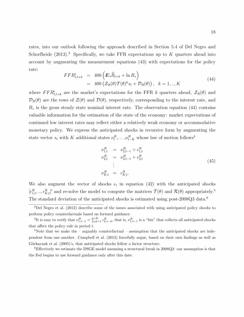
18

rates, into our outlook following the approach described in Section 5.4 of Del Negro and

Schorfheide (2013).3 Specifically, we take FFR expectations up to K quarters ahead into

account by augmenting the measurement equations (43) with expectations for the policy

rate:FFRe

t,t+k = 400(IEtRt+k + lnR∗

)= 400

(ZR(θ)T (θ)kst +DR(θ)

), k = 1, .., K

(44)

where FFRet,t+k are the market’s expectations for the FFR k quarters ahead, ZR(θ) and

DR(θ) are the rows of Z(θ) and D(θ), respectively, corresponding to the interest rate, and

R∗ is the gross steady state nominal interest rate. The observation equation (44) contains

valuable information for the estimation of the state of the economy: market expectations of

continued low interest rates may reflect either a relatively weak economy or accommodative

monetary policy. We express the anticipated shocks in recursive form by augmenting the

state vector st with K additional states νRt ,. . . ,νRt−K whose law of motion follows4

νR1,t = νR2,t−1 + εR1,t

νR2,t = νR3,t−1 + εR2,t...

νRK,t = εRK,t.

(45)

We also augment the vector of shocks εt in equation (42) with the anticipated shocks

[εR1,t, .., εRK,t]′ and re-solve the model to compute the matrices T (θ) and R(θ) appropriately.5

The standard deviation of the anticipated shocks is estimated using post-2008Q3 data.6

3Del Negro et al. (2012) describe some of the issues associated with using anticipated policy shocks to

perform policy counterfactuals based on forward guidance.4It is easy to verify that νR1,t−1 =

∑Kk=1 ε

Rk,t−k, that is, νR1,t−1 is a “bin” that collects all anticipated shocks

that affect the policy rule in period t.5Note that we make the – arguably counterfactual – assumption that the anticipated shocks are inde-

pendent from one another. Campbell et al. (2012) forcefully argue, based on their own findings as well as

Gurkaynak et al. (2005)’s, that anticipated shocks follow a factor structure.6Effectively we estimate the DSGE model assuming a structural break in 2008Q3: our assumption is that

the Fed begins to use forward guidance only after this date.

19

4 Priors and Posterior Estimates for the DSGE Model

Parameters

Table 1 shows the priors and posteriors for the DSGE model parameters. The top section

shows the prior for the policy rule parameters, namely the inflation target π∗, the responses

of interest rates to inflation (ψπ) and economic activity (ψy) – 4-quarter output growth in

the baseline specification – in the policy rule, persistence (ρr), and variance of i.i.d. policy

shocks, (σr). The prior on π∗ is centered at 2% in light of the Fed’s long run inflation

objective. Its posterior is slightly higher than 2%, reflecting the fact that inflation has been

higher on average than 2% in our sample.7 The priors on ψπ and ψy are centered at 2 and

0.2 respectively, and imply a fairly strong response to inflation and a moderate response to

output. The posterior means of these parameters are generally in line with the prior means,

although the posterior for ψπ is quite tighter than the prior (with 90% bands roughly between

1.9 and 2.4), indicating that the data are in agreement with a relatively strong reaction to

inflation in the interest feedback rule. The prior on the degree of inertia ρr is centered at 0.5

and is quite wide. The posterior estimates indicate a substantial degree of inertia (they are

centered at 0.8, with relatively tight bands), in line with the results in the literature. The

prior on the variance of the i.i.d. policy shocks σr is centered at 0.2.

Priors on nominal rigidities parameters ζp (prices) and ζw (wages) are shown in the second

panel of Table 1. We have considered two priors, as in Del Negro and Schorfheide (2008).

“Low Rigidities” (loosely calibrated at Bils and Klenow (2004) values of average duration

less than 2 quarters), and “High Rigidities” (duration about 4 quarters). The latter fits the

data better according to marginal likelihood criteria. Indeed the posterior distributions for

both ζp and ζw are higher than the prior, at about 0.9.

Priors on remaining parameters are shown in the bottom two panels of Table 1. The

priors on “Endogenous Propagation and Steady State”are generally chosen as in Del Negro

and Schorfheide (2008). The prior for the habit persistence parameter h is centered at 0.7,

which is the value used by Boldrin et al. (2001). The prior for a′′ implies that in response to

7In future model developments we plan to include in the model a time-varying inflation target. In order

to provide information on the public’s assessment of this time varying target we also plan to add the long

run inflation expectations to the list of observables, following the approach in Del Negro and Schorfheide

(2013).

20

a 1% increase in the return to capital, utilization rates rise by 0.1 to 0.3%. These numbers

are considerably smaller than the value used by Christiano et al. (2005). The 90% interval

for the prior distribution on νl implies that the Frisch labor supply elasticity lies between 0.3

and 1.3, reflecting the micro-level estimates at the lower end, and the estimates of Kimball

and Shapiro (2003) and Chang and Kim (2006) at the upper end. We use a pre-sample

of observations from 1959Q3-1984Q1 to choose the prior means for the parameters that

determine steady states.

For the credit frictions the key parameters are the elasticity of the spread with respect

to leverage, ζsp,b, the survival rate for the entrepreneurs, γe, and the steady state default

rate, F (ω). The last two are calibrated while the former is estimated. Following Gilchrist et

al. (2009), we set γe to 0.99. We set F (ω) to imply an annualized default rate of 3%, as in

Bernanke et al. (1999). The prior for the spread elasticity, ζsp,b, is a beta distribution with

mean 0.05 (as in Bernanke et al. (1999)) and standard deviation of 0.02. The steady state

spread has a Gaussian prior with mean 2 and standard deviation of 0.5, in annual percentage

terms.

The priors on the persistence of the exogenous processes are chosen as in Del Negro and

Schorfheide (2008). The priors on the standard deviations of the shocks are chosen so that

the overall variance of the endogenous variables is close to that observed in the pre-sample

1959Q3–1984Q1, informally following the approach in Del Negro and Schorfheide (2008).

5 The Transmission Mechanism and the Variance De-

composition

In this section, we illustrate some of the key economic mechanisms at work in the model’s

equilibrium. We do so with the aid of the impulse response functions and variance decom-

positions of the shocks hitting the economy, which we report in Figures 2 to 11.

We start the discussion from the shock most closely associated with the Great Recession

and the severe financial crisis that characterized it: the spread shock. As discussed above,

this shock stems from an increase in the perceived riskiness of borrowers, which induces

banks to charge higher interest rates for loans, thereby widening credit spreads. As a result

of this increase in the expected cost of capital, entrepreneurs’ borrowing falls, hindering their

21

ability to channel resources to the productive sector via capital accumulation. The model

identifies this shock by matching the behavior of the ratio of the Baa corporate bond yield

to the 10-year Treasury yield, and the spread’s comovement with output growth, inflation,

and the other observables.

Figure 2 shows the impulse responses of the variables used in the estimation to a one-

standard-deviation innovation in the spread shock. An innovation of this size increases the

observed spread by roughly 35 basis points and keeps it elevated for several quarters afterward

(bottom right panel). This dynamic profile is not too dissimilar from what was observed in

occasion of the Great Recession and its aftermath, when tighter financial conditions persisted

long after the official end of the recession, and arguably continue today, at least for some

borrowers.

This persistent increase in spreads leads to a reduction in investment and consequently

to a reduction in output growth (top left panel) and hours worked (top right panel). The fall

in the level of hours is fairly sharp in the first year and persists for many quarters afterwards,

leaving the labor input not much higher than at its trough four years after the impulse. Of

course, the effects of this same shock on GDP growth, which roughly mirrors that on the

level of hours, are more short-lived. Output growth returns to its steady state level about

two years after the shock hits, but it barely moves above it after that, implying a painfully

slow catch up of the level of GDP with its previous trend. The persistent drop in the level of

economic activity due to the spread shock also leads to a prolonged decline in real marginal

costs — which in this model map one-to-one into the labor share (middle left panel) — and,

via the New Keynesian Phillips curve, in inflation (middle right panel). Finally, policymakers

endogenously respond to the change in the inflation and real activity outlook by cutting the

federal funds rate (bottom left panel).

On average, the spread shock plays a limited role in fluctuations, as shown by the variance

decompositions in Figure 11. Exogenous changes in the spread account for no more than

10/15% of the variance of all variables — including the spread itself! — at any horizon. In

this respect, the Great Recession stands out as a very unusual event in our sample, due to

a very large and unlikely realization of the spread shock, as discussed in more detail in the

next section. In light of the impulse responses discussed above, which feature an extremely

gradual recovery of the real economy from this shock, the unusual “spread intensity” of the

Great Recession might help to explain the slow and halting nature of the lackluster recovery

22

that has followed it.

Very similar considerations hold for the MEI shock, which represents a direct hit to

the “technological” ability of entrepreneurs to transform investment goods into productive

capital, rather than an increase in their funding cost. Although the origins of the spread

and MEI shocks are different, the fact that they both affect the creation of new capital

implies very similar effects, but with opposite sign, on the observable variables, as shown by

the impulse responses in Figure 3. In particular, a positive MEI shock also implies a very

persistent increase in investment, output and hours worked, as well as in the labor share

and hence inflation. The key difference between the two impulses, which is also what allows

to tell them apart empirically, is that the MEI shock leaves spreads little changed (bottom

right panel). Moreover, MEI shocks play a fairly large role in fluctuations, accounting for

between 10% and 25% of the variance of the variables reported in Figure 11.

The TFP shock is another crucial shock in the model, with large contributions to the

variance of output, hours, the spread and (to a somewhat lesser extent) inflation and the

nominal interest rate. Unlike for the spread shock, this predominance is evident both un-

conditionally (Figure 11) and during the Great Recession, but much less over the course of

the recovery.

As shown in Figure 4, a positive TFP shock has a large and persistent effect on output

growth, even if the response of hours is muted in the first few quarters, and slightly negative

on impact, as in the data (see Galı (1999)). This muted response of hours is due to the

presence of nominal rigidities, which prevent aggregate demand from expanding sufficiently

to absorb the increased ability of the economy to supply output. With higher productivity,

marginal costs and thus the labor share fall, leading to lower inflation. The policy rule

specification implies that this negative correlation between inflation and real activity, which

is typical of supply shocks, produces countervailing forces on the interest rate, which as a

result moves little.

The last structural shock that plays a relevant role in the current economic environment

is the mark-up shock, whose impulse response is depicted in Figure 5. This shock is an

exogenous source of inflationary pressures, stemming from changes in the market power of

intermediate goods producers. As such, it leads to higher inflation and lower real activity,

as producers reduce supply to increase their desired markup. The effects of markup-shocks

are significantly less persistent than those of the other prominent supply shock in the model,

23

the TFP shock. GDP growth falls on impact after mark-ups increase, but returns above

average after about one year, thus restoring the original level of output over the horizon of

the simulation. Inflation is sharply higher for a couple of quarters, leading to a temporary

spike in the nominal interest rate, as monetary policy tries to limit the pass-through of the

shock to prices. Unlike in the case of TFP shocks, however, hours fall immediately, mirroring

the behavior of output.

The IRFs of the labor supply shock are depicted in Figure 6. This disturbance stands

at the opposite end of the spectrum with respect to the spread shock, in the sense that

its role in fluctuations is quite pronounced on average, but negligible in the last few years.

Labor shocks, which capture changes in households’ taste for leisure/work, are responsible

for about 20% of the fluctuations in most of the variables included in Figure 11. Their

dynamics feature a fairly persistent fall in hours worked (Figure 6), which triggers a fall

in output, but an increase in wages and the labor share, with the attendant inflationary

pressures and positive response of policy rates.

Finally, Figure 7 reports the IRFs of the government spending shock, which plays a very

limited quantitative role in the model, accounting for less than 5% of the fluctuations of all

variables, except at very short forecast horizons. In terms of dynamics, this shock boosts

GDP growth in the very short run, and hours for a few quarters, generating some mild

inflationary pressures that are kept in check by a rise in interest rates.

5.1 Policy Shocks: Anticipated and Unanticipated

Policy shocks deserve a separate treatment from the other structural disturbances in the

model, due to the presence of both standard (i.e. unanticipated) and less common, ‘antici-

pated’ shocks, which are known to agents in advance of their realization. Anticipated shocks

capture expected deviations of the interest rate from the setting implied by the policy rule,

which can occur in two different circumstances. First, such deviations are a way of capturing

in a linear model the contractionary effect of the zero lower bound on the nominal interest

rate, which prevents the policy rate from being negative when the policy rule would otherwise

dictate that it be. Second, anticipated shocks can capture communication on the part of the

central bank—the so-called “forward guidance”—whose objective is to shift expectations of

the future federal funds rate away from what would be implied by the historical policy rule,

24

for instance towards a more accommodative stance of policy, as is the case currently (see

Del Negro et al. (2012)).

Figure 8 reports the responses of the key variables to an unanticipated, negative 50 bps

monetary shock. The dynamics are those familiar from many VAR and DSGE studies. The

fall in the interest rate, which only gets reabsorbed over the course of two years, due mostly

to the persistence of the policy rule, leads to a sizable expansion in the real economy, with

hours increasing in a humped shaped pattern, by roughly 0.5% at the peak, and output

growth higher by 0.7% on impact, but returning to steady state in about one year. The

labor share also rises, with a similar pattern to that of hours, but its increase is more muted,

leading to a relatively modest, but fairly persistent increase in inflation. The spread falls on

impact, but it recovers afterward; its movements, however, are overall negligible.

Anticipated shocks have similar qualitative dynamics, in the sense of leading to an ex-

pansion in real activity and to more inflation, but with some peculiarities due to their effect

on expectations. Figures 9 and 10 plot IRFs for monetary policy shocks anticipated four

and eight quarters ahead, to give a flavor of the quantitative impact of anticipation. Shocks

anticipated at different horizons within the range considered in our exercises have similar

characteristics. The first feature that stands out in both responses is that an anticipated

negative shock (i.e. one that is expected to bring the interest rate down in the future), leads

to higher interest rates now. This is because the lower future interest rate has a stimulative

effect already today—agents are forward looking in the model. As a result, the policy rate

rises endogenously on impact in reaction to these positive real developments, as well as in

response to the associated higher inflation, as per the model’s Taylor rule. Nevertheless, the

economy continues to expand as the actual shock draws near and in fact it does not react

when the interest rate actually falls, since this development is old news at that point.

Another notable feature of the dynamics associated with these disturbances is that shocks

that occur in the future can have larger effects than contemporaneous ones of the same mag-

nitude (all three policy shocks are -50 bps in the figures). For instance, a shock anticipated

4 quarters ahead has a larger impact on GDP growth and hours than the contemporane-

ous shock (compare Figures 9 and 10), although the effect on these variables is somewhat

smaller for the 8-quarter-ahead shock. However, the impact on inflation is larger, the longer

is the anticipation horizon, since the effect on the labor share is more persistent, even if it

is smaller on impact. As a result, inflation, which discounts all feature developments in unit

25

labor costs, is higher immediately.

6 Developing a Narrative: from the Great Recession

to a Sluggish Recovery

In the previous section we have described the key mechanisms determining the equilibrium

evolution of the model. This transparent framework enables us to identify the source of

the past fluctuations and the current outlook for key economic indicators in terms of the

exogenous processes described above. In this section we describe how the model ‘explains’

the evolution of output growth, core PCE inflation and the federal funds rate (FFR) during

the Great Recession and what are the drivers behind their mean forecast through 2016.

Through the lenses of the model, the evolution of the economy since 2007 is driven by

two main forces. On the one hand, disruptions in the financial sector depressed aggregate

demand and employment, producing a sharp economic downturn and a sluggish recovery.

On the other hand, monetary policy played an important role in supporting the economy by

providing stimulus both by conventional measures at the onset of the recession and by the

use of forward guidance afterwards.

The importance of each shock for output growth, core PCE inflation, and the federal

funds rate (FFR) from 2007 on is quantified in Figure 12. In each of the three panels the

solid line (black for realized data, red for the mean forecast) shows the variable in deviation

from its steady state (for output growth and inflation, the numbers are quarter-to-quarter

annualized). The bars represent the contribution of each shock to the deviation of the

variable from steady state, that is, the counterfactual values of output growth, inflation, and

the federal funds rate (in deviations from the mean) obtained by setting all other shocks

to zero. By construction, for each observation the bars do in principle sum to the value on

the solid line. (To be precise, we do not show in the figure the contribution of the state at

the beginning of the sample on the subsequent evolution of the variables, as this deviation

from steady state contributes only modestly to short-term economic fluctuations.) The shock

decomposition and model forecasts shown in the figure are obtained using data up to 2013Q1,

the quarter for which we have the most recent GDP release, as well as the federal funds rate

and spread data for 2013Q2 (we use the average realizations for the quarter up to the forecast

date). In order to capture the effect of forward guidance, the federal funds rate expectations

26

in the model are constrained to be equal to market expectations for the federal funds rate

(as measured by OIS rates) until 2015Q2. Finally, we estimate the standard deviation of

the anticipated shocks as in Campbell et al. (2012), but we only use post-2008Q4 data. The

model forecasts represented by the red lines are distinct from the FR

The Great Recession was characterized by a severe financial crisis that impaired the flow

of credit, depressing aggregate demand and employment. The presence of credit intermedi-

ation frictions enables the FRBNY DSGE model to capture key dimensions of these events,

attributing an important part of the economic downturn to the spread shock, which reflects

higher perceived riskiness of borrowers and causes disruptions in financial intermediation.

In fact, Figure 12 shows that spread shocks (measured by the dark purple bars) explain

about half of the drop in output growth and inflation during the recession. As we discussed,

this shock works through the model by increasing the expected cost of capital and reducing

entrepreneurs’ borrowing: hence it decreases their capital accumulation and their ability to

channel resources to the productive sector. Figure 14 plots the standardized innovations

(that is, the innovations measured in standard deviation units) of the shocks in the model,

from 2007 on. The figure shows that realizations of the spread shock are indeed positive

in the early part of the Great Recession, with large spikes in late 2007 and particularly in

2008Q4, in the aftermath of the Lehman collapse.

Other shocks also contributed to the Great Recession. Figure 12 shows that TFP shocks

(dark red bars) played an important role in the decline of output, particularly in 2008. As

revealed in Figure 14, TFP shocks were indeed largely negative during this period, reflecting

disruptions in production for given factor inputs. However, productivity shocks cannot fully

account for the Great Recession because a drop in productivity leads to an increase in

inflation, rather than the decline that was observed. This is evident from Figure 4, which

shows the impulse responses to a one-standard-deviation positive TFP shock. One can infer

from this figure that a negative one-standard deviation TFP shock would lead to a substantial

drop in output but also to an increase in inflation. Moreover, because of nominal rigidities,

the impact response of hours worked to the negative shock in productivity is very small, if

not positive.

“Labor supply” shocks (pink bars) have not been major driver of the Great Recession,

as they cannot replicate the observed comovement between inflation and output during this

episode. As we discussed (see also Figure 6) positive labor supply shocks (exogenous inward

27

shifts in labor supply, possibly due to unmodeled labor market imperfections) lead to a

decline in output and hours, but to an increase in inflation. This is because firms’ marginal

costs rise following a contraction in labor supply.

Monetary policy shocks played an important countervailing role during the recession

(orange bars). Offsetting the negative effect of spread shocks and TFP shocks, monetary

policy contributed to lifting GDP growth by more than two percentage points in late 2007

and in the first half of 2008, by sharply reducing the Federal funds rate. As shown in the

bottom panel, the reduction in the federal funds rate observed in the recession was much

larger than explained by the contraction in inflation and output growth. Hence, the model

identifies a series of negative monetary policy shocks as the primary drivers of the rate’s

sharp decline by the end of 2008. The large drop in interest rates boosted output growth

and, albeit with a lag, had a positive effect on inflation.

Moving past the Great Recession, Figure 12 shows that the economy continues to be

affected by the headwinds from the financial crisis. These are captured initially by the

effects of the spread shocks and later by MEI shocks (azure bars), which maintain the

recovery subdued, real marginal costs low, and inflation consequently low. Accommodative

monetary policy, and particularly forward guidance about the future path of the federal

funds rate (captured here by anticipated policy shocks) has played an important role in

counteracting the financial headwinds, and in lifting up output and inflation.

In more detail, the role played by spread and MEI shocks is quite evident in the shock

decomposition for inflation and interest rates, which shows that MEI, and to a lesser extent,

spread shocks play a key role in keeping these two variables below steady state. This feature

of the DSGE forecast is less evident for real output growth, as the contribution of MEI

shocks seems small, particularly toward the end of the forecast horizon, and the contribution

of spread shocks is negligible (and positive). However, recall that a small, but still negative,

effect on output growth implies that the effect of the MEI shocks on the level of output is

getting larger, even several quarters after the occurrence of the shock. Similarly, the fact

that the growth impact of spread shocks is positive but very small implies that the level of

output is very slowly returning to trend. This is evident in the protracted effect of spread

and MEI shocks on aggregate hours, shown in the impulse responses of Figures 2 and 3,

respectively, and discussed above. In turn, the fact that economic activity is well below

trend pushes inflation and consequently interest rates (given the Fed’s reaction function)

28

below steady state.

After the end of the Great Recession, monetary policy continued to stimulate output

growth from mid 2009 to late 2012 through anticipated monetary policy shocks, representing

the use of forward guidance. Since shocks at different horizons interact with one another, it

is difficult to assess their overall impact. It is therefore more useful to show their cumulative

impact, as shown by the orange bars in Figure 12. One can see that the cumulative impact of

policy shocks on the interest rate is currently very small, implying that the level of the interest

rate is not too far from that implied by the estimated policy rule. Later in the forecast horizon

the impact of these shocks becomes larger, and reaches almost one percentage point in 2015:

the impact of the forward guidance, combined with the interest rate smoothing component

of the policy, which limits quarter-to-quarter adjustments, implies that the renormalization

path is lower than that implied by the estimated rule.

Despite the important role played by policy shocks in pushing inflation and output

upward both in the immediate aftermath of the recession and in the current period, the

impact of policy on the level of output has started to wane by the end of 2012. This implies

that the effect of policy on growth is actually negative after that, which explains why growth

is still at or below trend by the end of 2016. This is partly because the stimulative effect

of the forward guidance is front-loaded, and hence has the largest impact when it is first

implemented.

Finally, given the weak outlook for marginal costs, the model attributes much of the

rise in core inflation in 2011 and in early 2012 to price mark-up shocks. Increases in mark-

ups in our monopolistically competitive setting push inflation above marginal costs and

reduce output. Figure 5 shows that mark-up shocks capture large but transitory movements

in inflation, such as those due to oil price fluctuations. However with the moderation in

energy prices since then, mark-up shocks have had much smaller effects on inflation in recent

quarters, and play almost no role in the inflation forecasts. Since output is returning to trend

following mark-up shocks, these actually contribute positively to output growth from 2013

onward.

29

7 The Forecast Distributions

The previous section described the model forecast for key economic variables. An additional

advantage of using structural economic models for forecasting and policy analysis is the

ability to produce an entire forecast distribution, which reflects uncertainty about both

structural parameters and the state of the economy. Figure 13 presents quarterly forecasts

for output growth, core PCE inflation and the federal funds rate. In the graphs, the black

line represents data, the red line indicates the mean forecast, and the shaded areas mark

the uncertainty associated with our forecasts as 50, 60, 70, 80 and 90 percent probability

intervals. Output growth and inflation are expressed in terms of percent annualized rates,

quarter to quarter. The interest rate is the annualized quarterly average. The bands reflect

both parameter uncertainty and shock uncertainty.

As discussed above, the model still projects a lackluster recovery in economic activity,

with output growth in the neighborhood of 2 percent throughout the forecast horizon. There

is moderate uncertainty around the real GDP forecasts; for example the 70 percent bands

cover the interval -1.7 to 5.2 percent in 2014. Concerning the core PCE inflation forecast,

the model predicts a very slow return to the long-run FOMC target over the forecasting

horizon: indeed, according to the mean forecast, inflation is still below 2 percent in 2017.

The 70 percent probability bands for inflation in 2014, 2015, and 2016 are within the 0.6-2.8

percent interval, implying that the model places high probability on inflation realizations

below the long-run FOMC target.

8 An Assessment of the Model’s Real-Time Forecasts,

2010-2012

In this section we discuss the real-time forecasts from the FRBNY-DSGE model starting

from March 2010, when we began producing forecasts, and provide a broad assessment

of how the DSGE model has fared so far in terms of forecasting accuracy. The forecasts

have been produced roughly eight times a year, about two weeks before each Federal Open

Markets Committee meeting, and have all been published in internal documents. We should

emphasize that the model specification has changed over time, reflecting model developments.

For instance, financial frictions which, as discussed above, play a crucial role in explaining the

30

Great Recession and in shaping the current forecast, were introduced in 2011. Concerning our

assumptions about monetary policy, the horizon for which we use market-based observations

on FFR expectations in order to take forward guidance into account has changed over time.

We present two sets of graphs. Figure 16 shows, for the period 2010-2012, three vintages

of the annualized quarterly forecasts for output growth and core PCE inflation from the

DSGE model. For comparison, the figure shows also the median forecast of the Federal

Reserve Bank of Philadelphia’s Survey of Professional Forecasters (SPF), indicated by red

lines. We report the last forecast vintage generated for each year so that SPF forecasts

have the longest possible forecast horizon. Importantly, all vintages of SPF forecasts are

produced after the DSGE forecast is produced; hence the DGSE econometricians are always

at an informational disadvantage relative to the other forecasters.

We show two types of DSGE forecasts. The first, which we refer to as “unconditional”

forecasts and which are indicated by dark blue lines are constructed as described in the

previous section, by using the most recently-available released data, including up-to-date

spread and FFR data. The second forecast, which we refer to as “conditional” and which is

indicated by light blue lines incorporates the FRBNY staff nowcast for the current quarter,

and treats it as actual data. (The forecast is conditioned on the FRBNY staff nowcast in the

spirit of Doan et al. (1984), hence the adjective “conditional”). This second forecast partly

overcomes the informational disadvantage mentioned above (see the discussion in Del Negro

and Schorfheide (2013)).

Figure 17 shows the rolling progression over time of forecasts for year-over-year output

growth and Q4/Q4 core PCE inflation in 2011, 2012, and 2013. We show these yearly

forecasts because they allow for a comparison with SPF forecasts for longer horizons than

the quarterly forecasts.

From both sets of figures we can see that in the periods considered the FRBNY-DSGE

output growth forecasts have been comparable to, if not better than, the median SPF fore-

casts. To some extent the SPF has been overly optimistic about growth, especially in the

medium-long term, as professional forecasters have been repeatedly forecasting a relatively

rapid closing of the output gap which opened in the aftermath of the financial crisis. Con-

versely, the DSGE model has been consistently predicting a very slow recovery following

financial shocks, as discussed at length in previous sections. As a consequence, we can see

from Figure 17 that for each of the years considered, the SPF has initially produced an overly

31

optimistic forecast, which, as time passes and more information is accumulated, converges

to where the DSGE model had been all along. (Note that the apparent mis-forecasting in

2012 by all models is due to the July 2013 comprehensive NIPA revision which revised up

the growth rate of real GDP from 2.2% to 2.8%.) However, the DSGE model continues to

predict rather weak growth forecasts several years after the financial crisis, and we suspect

that these weak forecasts may partly result from the DSGE model “overfitting” the crisis.

The DGSE model, on the other hand, under-forecasted inflation in 2011 and early 2012,

partly because it missed the effect of commodity prices on core inflation, and partly because

the weak activity forecast within the model naturally translate into a weak inflation forecast.

We can see, however, that in late 2012 and 2013, after the effect of commodity prices waned,

inflation has fallen and is now broadly in line with, say, the DSGE model forecasts made in

2010.

9 Conclusion

In this paper, we presented the FRBNY DSGE model and discussed how it is used for

forecasting and to interpret the recent history. At the FRBNY, the model has also been

used for policy analysis, for example as discussed in Del Negro et al. (2012). In addition,

we have used the model to evaluate the impact on the outlook of adopting monetary policy

rules that differ from the historical one.

We have focused our discussion on one model only. We are well aware that in presence of

model misspecification one would want to consider multiple models (see Geweke and Amisano

(2012)). These models may differ in terms of their underlying assumptions, estimation

procedures, and degrees of theoretical coherence (as measured by the tightness with which

the cross-equations are imposed, e.g. see Del Negro and Schorfheide (2004)). This is an

important direction for future research and modeling work within a central bank.

In terms of modelling, there are many directions in which the model could be enriched

or adjusted, to make it an even more useful tool for day-to-day monetary policy analysis. In

particular, it would be desirable to include a more fully developed model of the labor market,

which would account for the unemployment rate, given the importance of this variable in

the policy debate. Incorporating a more fundamental role for financial intermediation, in

32

particular as a potential source of economic instability, as well as developing the asset pricing

implications of the model, would also help it better answer some of the questions often on

the minds of policymakers.

33

References

An, Sungbae and Frank Schorfheide, “Bayesian Analysis of DSGE Models,” Economet-

ric Reviews, 2007, 26 (2-4), 113–172.

Bernanke, Ben, Mark Gertler, and Simon Gilchrist, “The Financial Accelerator in a

Quantitative Business Cycle Framework,” in John B. Taylor and Michael Woodford, eds.,

Handbook of Macroeconomics, Vol. 1C, North Holland, Amsterdam, 1999.

Bils, Mark and Peter Klenow, “Some Evidence on the Importance of Sticky Prices,”

Journal of Political Economy, 2004, 112, 947–985.

Boldrin, Michele, Lawrence Christiano, and Jonas Fisher, “Habit Persistence, Asset

Returns, and the Business Cycle,” American Economic Review, 2001, 91, 149–166.

Calvo, Guillermo, “Staggered Prices in a Utility Maximizing Framework,” Journal of

Monetary Economics, 1983, 12 (3), 383–398.

Campbell, Jeffrey R., Jonas D.M. Fisher, and Alejandro Justiniano, “Monetary

Policy Forward Guidance and the Business Cycle,” Federal Reserve Bank of Chicago Work-

ing Paper, 2012.

Chang, Youngsun and Sun-Bin Kim, “Individual to Aggregate Labor Supply: A Quan-

titative Analysis based on Heterogeneous Agent Macroeconomy,” International Economic

Review, 2006, 47, 1–27.

Christiano, Lawrence J., Martin Eichenbaum, and Charles L. Evans, “Nominal

Rigidities and the Dynamic Effects of a Shock to Monetary Policy,” Journal of Political

Economy, 2005, 113, 1–45.

, Roberto Motto, and Massimo Rostagno, “Financial Factors in Economic Fluctua-

tions,” Manuscript, Northwestern University and European Central Bank, 2009.

Del Negro, Marco and Frank Schorfheide, “Priors from General Equilibrium Models

for VARs,” International Economic Review, 2004, 45 (2), 643 – 673.

and , “Forming Priors for DSGE Models (and How it Affects the Assessment of Nominal

Rigidities),” Journal of Monetary Economics, 2008, 55 (7), 1191–1208.

34

and , “Bayesian Macroeconometrics,” in Herman K. van Dijk, Gary Koop, and John

Geweke, eds., Handbook of Bayesian Econometrics, Oxford University Press, 2010.

and , “DSGE Model-Based Forecasting,” in Graham Elliott and Allan Timmermann,

eds., Handbook of Economic Forecasting, Volume 2, Elsevier, 2013.

, Marc Giannoni, and Christina Patterson, “The Forward Guidance Puzzle,” Federal

Reserve Bank of New York Staff Report, 2012.

Doan, Thomas, Robert Litterman, and Christopher A. Sims, “Forecasting and Con-

ditional Projections Using Realistic Prior Distributions,” Econometric Reviews, December

1984, 3 (4), 1–100.

Galı, Jordi, “Technology, Employment, and the Business Cycle: Do Technology Shocks

Explain Aggregate Fluctuations?,” American Economic Review, 1999, 89 (1), 249 – 271.

Geweke, John and Gianni Amisano, “Prediction with Misspecified Models,” American

Economic Review: Papers & Proceedings, 2012, 103 (3), 482–486.

Gilchrist, Simon, Alberto Ortiz, and Egon Zakrajsek, “Credit Risk and the Macroe-

conomy: Evidence from an Estimated DSGE Model,” Unpublished, July 2009.

Gurkaynak, Refet S., Brian Sack, and Eric T. Swanson, “Do actions speak louder

than words? The response of asset prices to monetary policy actions and statements.,”

International Journal of Central Banking, 2005, 1 (1), 55–93.

Justiniano, Alejandro, Giorgio E. Primiceri, and Andrea Tambalotti, “Investment

Shocks and Business Cycles,” Journal of Monetary Economics, 2010, 57 (2), 132145.

Kimball, Miles and Matthew Shapiro, “Labor Supply: Are the Income and Substitution

Effects Both Large or Both Small?,” Manuscript, University of Michigan, 2003.

Sbordone, Argia M., Andrea Tambalotti, Rao Krishna, and Kieran Walsh, “Pol-

icy Analysis Using DSGE Models: An Introduction,” FRBNY Economic Policy Review,

October 2010, 16 (2), 23–43.

Sims, Christopher A., “Solving Linear Rational Expectations Models,” Computational

Economics, 2002, 20 ((1-2)), 1–20.

35

Smets, Frank and Raf Wouters, “Shocks and Frictions in US Business Cycles: A

Bayesian DSGE Approach,” American Economic Review, 2007, 97 (3), 586 – 606.

36

Table 1: Prior and Posterior for the DSGE Model Parameters

Parameters Prior Mean Prior Stdd Post Mean 90% Lower Band 90% Upper Band

Policy Parameters

π∗ 2.000 0.250 2.392 2.128 2.651

ψπ 2.000 0.250 2.132 1.869 2.384

ψy 0.200 0.100 0.253 0.151 0.360

ρr 0.500 0.200 0.800 0.763 0.836

σr 0.200 4.000 0.139 0.124 0.156

Nominal Rigidities Parameters

ζp 0.750 0.100 0.878 0.853 0.904

ζw 0.750 0.100 0.902 0.870 0.933

Other “Endogenous Propagation and Steady State” Parameters

α 0.330 0.020 0.351 0.346 0.356

a′′ 0.200 0.100 0.286 0.119 0.452

h 0.700 0.050 0.730 0.671 0.790

S′′ 4.000 1.500 4.013 2.986 5.056

νl 2.000 0.750 1.310 0.502 2.052

r∗ 1.500 1.000 0.305 0.046 0.557

γ 2.750 0.500 1.726 1.331 2.095

g∗ 0.300 0.100 0.185 0.086 0.282

ζsp,b 0.050 0.020 0.081 0.048 0.112

SP∗ 2.000 0.500 1.112 0.738 1.474

ρs and σs

ρz 0.400 0.250 0.473 0.344 0.607

ρφ 0.750 0.150 0.308 0.188 0.428

ρλf0.750 0.150 0.500 0.400 0.606

ρµ 0.750 0.150 0.994 0.989 1.000

ρg 0.750 0.150 0.931 0.849 0.999

ρσw 0.750 0.150 0.960 0.931 0.991

σz 0.300 4.000 0.778 0.686 0.867

σφ 3.000 4.000 29.082 13.474 44.661

σλf0.200 4.000 0.084 0.069 0.098

σµ 0.750 4.000 0.356 0.271 0.438

σg 0.500 4.000 0.226 0.178 0.271

σσw0.050 4.000 0.084 0.074 0.093

Note: The values reported for the parameters π∗, r∗, γ, and SP∗ are expressed in annualized terms. Thefollowing parameters are fixed: δ = 0.025, νm = 2, λw = 0.3, χ = 0.1, λf = 0.15, F (ω) = 0.0075, γe =0.99.

37

Figure 1: Model Structure

Households

habit

persistence

labor

wage

rigidities

labor supply

shocks

Firms

productivity shocks

intermediate goods

price

rigiditiesmark-upshocks

Final GoodsProducers

consumption

investment

CapitalProducers

MEI

shocks

investmentadjustment

costs

deposits

Banksloans

credit

frictions

spread shocks

Entrepreneurs

capital

utilization

bills

Government

interest rate

policy

policy

shocksgov’t spending

shocks

38

Figure 2: Responses to a Spread Shock

0 4 8 12−0.8

−0.6

−0.4

−0.2

0

0.2Output Growth

Per

cent

Ann

ualiz

ed

0 4 8 12−0.8

−0.6

−0.4

−0.2

0Aggregate Hours

Per

cent

Ann

ualiz

ed

0 4 8 12−0.2

−0.15

−0.1

−0.05

0Labor Share

Per

cent

0 4 8 12−0.15

−0.1

−0.05

0

0.05Core PCE Inflation

Per

cent

Ann

ualiz

ed

0 4 8 12−0.25

−0.2

−0.15

−0.1

−0.05

0Interest Rate

Per

cent

Ann

ualiz

ed

0 4 8 120

0.1

0.2

0.3

0.4Spread

Per

cent

Ann

ualiz

ed

39

Figure 3: Responses to an MEI Shock

0 4 8 120

0.5

1

1.5Output Growth

Per

cent

Ann

ualiz

ed

0 4 8 120

0.2

0.4

0.6

0.8

1Aggregate Hours

Per

cent

Ann

ualiz

ed

0 4 8 120

0.05

0.1

0.15

0.2

0.25Labor Share

Per

cent

0 4 8 120

0.05

0.1

0.15

0.2

0.25Core PCE Inflation

Per

cent

Ann

ualiz

ed

0 4 8 120

0.1

0.2

0.3

0.4Interest Rate

Per

cent

Ann

ualiz

ed

0 4 8 120

0.05

0.1

0.15

0.2Spread

Per

cent

Ann

ualiz

ed

40

Figure 4: Responses to a TFP Shock

0 4 8 12−0.5

0

0.5

1

1.5

2Output Growth

Per

cent

Ann

ualiz

ed

0 4 8 12−0.5

0

0.5

1

1.5Aggregate Hours

Per

cent

Ann

ualiz

ed

0 4 8 12−0.8

−0.6

−0.4

−0.2

0

0.2Labor Share

Per

cent

0 4 8 12−0.3

−0.2

−0.1

0

0.1Core PCE Inflation

Per

cent

Ann

ualiz

ed

0 4 8 12−0.05

0

0.05

0.1

0.15Interest Rate

Per

cent

Ann

ualiz

ed

0 4 8 120

0.02

0.04

0.06

0.08Spread

Per

cent

Ann

ualiz

ed

41

Figure 5: Responses to a Mark-up Shock

0 4 8 12−0.8

−0.6

−0.4

−0.2

0

0.2Output Growth

Per

cent

Ann

ualiz

ed

0 4 8 12−0.6

−0.4

−0.2

0

0.2Aggregate Hours

Per

cent

Ann

ualiz

ed

0 4 8 12−0.4

−0.3

−0.2

−0.1

0Labor Share

Per

cent

0 4 8 12−0.2

0

0.2

0.4

0.6

0.8Core PCE Inflation

Per

cent

Ann

ualiz

ed

0 4 8 12−0.1

0

0.1

0.2

0.3Interest Rate

Per

cent

Ann

ualiz

ed

0 4 8 12−0.02

−0.01

0

0.01Spread

Per

cent

Ann

ualiz

ed

42

Figure 6: Responses to a Labor Supply Shock

0 4 8 12−0.8

−0.6

−0.4

−0.2

0

0.2Output Growth

Per

cent

Ann

ualiz

ed

0 4 8 12−1.5

−1

−0.5

0Aggregate Hours

Per

cent

Ann

ualiz

ed

0 4 8 12−0.2

0

0.2

0.4

0.6Labor Share

Per

cent

0 4 8 120

0.05

0.1

0.15

0.2

0.25Core PCE Inflation

Per

cent

Ann

ualiz

ed

0 4 8 120

0.05

0.1

0.15

0.2Interest Rate

Per

cent

Ann

ualiz

ed

0 4 8 12−0.08

−0.06

−0.04

−0.02

0Spread

Per

cent

Ann

ualiz

ed

43

Figure 7: Responses to a Government Spending Shock

0 4 8 12−0.5

0

0.5

1Output Growth

Per

cent

Ann

ualiz

ed

0 4 8 120

0.1

0.2

0.3

0.4Aggregate Hours

Per

cent

Ann

ualiz

ed

0 4 8 120

0.05

0.1

0.15

0.2Labor Share

Per

cent

0 4 8 120

0.01

0.02

0.03

0.04

0.05Core PCE Inflation

Per

cent

Ann

ualiz

ed

0 4 8 120

0.02

0.04

0.06

0.08Interest Rate

Per

cent

Ann

ualiz

ed

0 4 8 12−0.02

−0.015

−0.01

−0.005

0Spread

Per

cent

Ann

ualiz

ed

44

Figure 8: Responses to a Monetary Policy Shock (-50 bps)

0 4 8 12−0.2

0

0.2

0.4

0.6

0.8Output Growth

Per

cent

Ann

ualiz

ed

0 4 8 120

0.2

0.4

0.6

0.8Aggregate Hours

Per

cent

Ann

ualiz

ed

0 4 8 120

0.05

0.1

0.15

0.2Labor Share

Per

cent

0 4 8 12−0.02

0

0.02

0.04

0.06

0.08Core PCE Inflation

Per

cent

Ann

ualiz

ed

0 4 8 12−0.5

−0.4

−0.3

−0.2

−0.1

0Interest Rate

Per

cent

Ann

ualiz

ed

0 4 8 12−0.02

−0.01

0

0.01

0.02

0.03Spread

Per

cent

Ann

ualiz

ed

45

Figure 9: Responses to a 4Q Ahead Anticipated Monetary Policy Shock (-50 bps)

0 4 8 12−0.5

0

0.5

1Output Growth

Per

cent

Ann

ualiz

ed

0 4 8 120

0.2

0.4

0.6

0.8

1Aggregate Hours

Per

cent

Ann

ualiz

ed

0 4 8 120

0.1

0.2

0.3

0.4Labor Share

Per

cent

0 4 8 12−0.05

0

0.05

0.1

0.15Core PCE Inflation

Per

cent

Ann

ualiz

ed

0 4 8 12−0.4

−0.2

0

0.2

0.4Interest Rate

Per

cent

Ann

ualiz

ed

0 4 8 12−0.02

0

0.02

0.04

0.06Spread

Per

cent

Ann

ualiz

ed

46

Figure 10: Responses to a 8Q Ahead Anticipated Monetary Policy Shock (-50 bps)

0 4 8 12−0.5

0

0.5

1Output Growth

Per

cent

Ann

ualiz

ed

0 4 8 120

0.5

1

1.5Aggregate Hours

Per

cent

Ann

ualiz

ed

0 4 8 120

0.05

0.1

0.15

0.2

0.25Labor Share

Per

cent

0 4 8 12−0.05

0

0.05

0.1

0.15

0.2Core PCE Inflation

Per

cent

Ann

ualiz

ed

0 4 8 12−0.4

−0.2

0

0.2

0.4Interest Rate

Per

cent

Ann

ualiz

ed

0 4 8 12−0.02

0

0.02

0.04

0.06Spread

Per

cent

Ann

ualiz

ed

47

Figure 11: Variance Decomposition

Quarters Ahead

Per

cent

Output Growth

4 8 12 16 20 24 28 32 36 40 inf0

0.2

0.4

0.6

0.8

1

0

0.2

0.4

0.6

0.8

1

Quarters Ahead

Per

cent

Core PCE Inflation

4 8 12 16 20 24 28 32 36 40 inf0

0.2

0.4

0.6

0.8

1

0

0.2

0.4

0.6

0.8

1

Quarters Ahead

Per

cent

Interest Rate

4 8 12 16 20 24 28 32 36 40 inf0

0.2

0.4

0.6

0.8

1

Spread MEI TFP Policy Mark−Up Gov’t Labor

0

0.2

0.4

0.6

0.8

1

48

Figure 12: Shock Decomposition

2007 2008 2009 2010 2011 2012 2013 2014 2015 2016 2017−12

−10

−8

−6

−4

−2

0

2

4

Per

cent

Q−t

o−Q

Ann

ualiz

ed

−12

−10

−8

−6

−4

−2

0

2

4

Output Growth(deviations from mean)

2007 2008 2009 2010 2011 2012 2013 2014 2015 2016 2017−2

−1

0

1

2

Per

cent

Q−t

o−Q

Ann

ualiz

ed

−2

−1

0

1

2

Core PCE Inflation(deviations from mean)

2007 2008 2009 2010 2011 2012 2013 2014 2015 2016 2017−5

−4

−3

−2

−1

0

1

2

Per

cent

Q−t

o−Q

Ann

ualiz

ed

Spread MEI TFP Policy Mark−Up Gov’t Labor

−5

−4

−3

−2

−1

0

1

2

Interest Rate(deviations from mean)

The shock decomposition is presented for the realized data as well as the forecast. The solid lines (black for realized data, red

for mean forecast) show each variable in deviation from its steady state. The bars represent the shock contributions; specifically,

the bars for each shock represent the counterfactual values for the observables (in deviations from the mean) obtained by setting

all other shocks to zero.

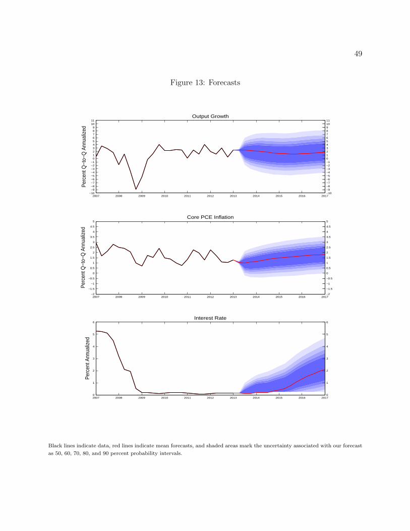
49

Figure 13: Forecasts

2007 2008 2009 2010 2011 2012 2013 2014 2015 2016 2017−10−9−8−7−6−5−4−3−2−1

0123456789

1011

Per

cent

Q−t

o−Q

Ann

ualiz

ed

2007 2008 2009 2010 2011 2012 2013 2014 2015 2016 2017−2

−1.5

−1

−0.5

0

0.5

1

1.5

2

2.5

3

3.5

4

4.5

5

Per

cent

Q−t

o−Q

Ann

ualiz

ed

2007 2008 2009 2010 2011 2012 2013 2014 2015 2016 20170

1

2

3

4

5

6

Per

cent

Ann

ualiz

ed

Output Growth

−10−9−8−7−6−5−4−3−2−101234567891011

Core PCE Inflation

−2

−1.5

−1

−0.5

0

0.5

1

1.5

2

2.5

3

3.5

4

4.5

5

Interest Rate

0

1

2

3

4

5

6

Black lines indicate data, red lines indicate mean forecasts, and shaded areas mark the uncertainty associated with our forecast

as 50, 60, 70, 80, and 90 percent probability intervals.

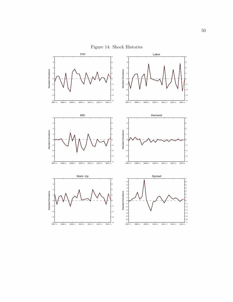
50

Figure 14: Shock Histories

2007−1 2008−1 2009−1 2010−1 2011−1 2012−1 2013−1−4

−3

−2

−1

0

1

2

3

4

Sta

ndar

d D

evia

tions

−4

−3

−2

−1

0

1

2

3

4TFP

2007−1 2008−1 2009−1 2010−1 2011−1 2012−1 2013−1−4

−3

−2

−1

0

1

2

3

4

Sta

ndar

d D

evia

tions

−4

−3

−2

−1

0

1

2

3

4Labor

2007−1 2008−1 2009−1 2010−1 2011−1 2012−1 2013−1−4

−3

−2

−1

0

1

2

3

4

Sta

ndar

d D

evia

tions

−4

−3

−2

−1

0

1

2

3

4MEI

2007−1 2008−1 2009−1 2010−1 2011−1 2012−1 2013−1−4

−3

−2

−1

0

1

2

3

4

Sta

ndar

d D

evia

tions

−4

−3

−2

−1

0

1

2

3

4Demand

2007−1 2008−1 2009−1 2010−1 2011−1 2012−1 2013−1−4

−3

−2

−1

0

1

2

3

4

Sta

ndar

d D

evia

tions

−4

−3

−2

−1

0

1

2

3

4Mark−Up

2007−1 2008−1 2009−1 2010−1 2011−1 2012−1 2013−1−7

−6

−5

−4

−3

−2

−1

0

1

2

3

4

5

6

7

Sta

ndar

d D

evia

tions

−7

−6

−5

−4

−3

−2

−1

0

1

2

3

4

5

6

7Spread

51

Figure 15: Anticipated Shock Histories

2007−1 2008−1 2009−1 2010−1 2011−1 2012−1 2013−1−0.4

−0.3

−0.2

−0.1

0

0.1

0.2

Per

cent

−0.4

−0.3

−0.2

−0.1

0

0.1

0.2Money

2007−1 2008−1 2009−1 2010−1 2011−1 2012−1 2013−1−0.4

−0.3

−0.2

−0.1

0

0.1

0.2

Per

cent

−0.4

−0.3

−0.2

−0.1

0

0.1

0.2Ant 1

2007−1 2008−1 2009−1 2010−1 2011−1 2012−1 2013−1−0.4

−0.3

−0.2

−0.1

0

0.1

0.2

Per

cent

−0.4

−0.3

−0.2

−0.1

0

0.1

0.2Ant 2

2007−1 2008−1 2009−1 2010−1 2011−1 2012−1 2013−1−0.4

−0.3

−0.2

−0.1

0

0.1

0.2

Per

cent

−0.4

−0.3

−0.2

−0.1

0

0.1

0.2Ant 3

2007−1 2008−1 2009−1 2010−1 2011−1 2012−1 2013−1−0.4

−0.3

−0.2

−0.1

0

0.1

0.2

Per

cent

−0.4

−0.3

−0.2

−0.1

0

0.1

0.2Ant 4

2007−1 2008−1 2009−1 2010−1 2011−1 2012−1 2013−1−0.4

−0.3

−0.2

−0.1

0

0.1

0.2

Per

cent

−0.4

−0.3

−0.2

−0.1

0

0.1

0.2Ant 5

2007−1 2008−1 2009−1 2010−1 2011−1 2012−1 2013−1−0.4

−0.3

−0.2

−0.1

0

0.1

0.2

Per

cent

−0.4

−0.3

−0.2

−0.1

0

0.1

0.2Ant 6

2007−1 2008−1 2009−1 2010−1 2011−1 2012−1 2013−1−0.4

−0.3

−0.2

−0.1

0

0.1

0.2

Per

cent

−0.4

−0.3

−0.2

−0.1

0

0.1

0.2Ant 7

2007−1 2008−1 2009−1 2010−1 2011−1 2012−1 2013−1−0.4

−0.3

−0.2

−0.1

0

0.1

0.2

Per

cent

−0.4

−0.3

−0.2

−0.1

0

0.1

0.2Ant 8

2007−1 2008−1 2009−1 2010−1 2011−1 2012−1 2013−1−0.4

−0.3

−0.2

−0.1

0

0.1

0.2

Per

cent

−0.4

−0.3

−0.2

−0.1

0

0.1

0.2Ant 9

52

Figure 16: Real-Time Forecasts

November 2010

2009 2010 2011 2012 2013 2014−3

−2

−1

0

1

2

3

4

5

6

7Output Growth

Per

cent

Q−t

o−Q

ann

ualiz

ed

DSGE UnconditionalDSGE ConditionalSPF (Median)

2009 2010 2011 2012 2013 20140

0.5

1

1.5

2

2.5

3Core PCE Inflation

Per

cent

Q−t

o−Q

ann

ualiz

ed

DSGE UnconditionalDSGE ConditionalSPF (Median)

October 2011

2009 2010 2011 2012 2013 2014−3

−2

−1

0

1

2

3

4

5

6

7Output Growth

Per

cent

Q−t

o−Q

ann

ualiz

ed

DSGE UnconditionalDSGE ConditionalSPF (Median)

2009 2010 2011 2012 2013 20140

0.5

1

1.5

2

2.5

3Core PCE Inflation

Per

cent

Q−t

o−Q

ann

ualiz

ed

DSGE UnconditionalDSGE ConditionalSPF (Median)

November 2012

2009 2010 2011 2012 2013 2014 2015 2016−3

−2

−1

0

1

2

3

4

5

6

7Output Growth

Per

cent

Q−t

o−Q

ann

ualiz

ed

DSGE UnconditionalDSGE ConditionalSPF (Median)

2009 2010 2011 2012 2013 2014 2015 20160

0.5

1

1.5

2

2.5

3Core PCE Inflation

Per

cent

Q−t

o−Q

ann

ualiz

ed

DSGE UnconditionalDSGE ConditionalSPF (Median)

53

Figure 17: Real-Time Forecast Progression

Year-over-year Output Growth Q4/Q4 Core PCE Inflation

2010.03 2010.08 2010.11 2011.03 2011.06 2011.1 2012.010

0.5

1

1.5

2

2.5

3

3.5

4

4.5

5

Vintage

2011

Yea

r−ov

er−y

ear O

utpu

t Gro

wth

DSGE UnconditionalDSGE ConditionalSPF (Median)Actual

2010.03 2010.08 2010.11 2011.03 2011.06 2011.1 2012.010

0.5

1

1.5

2

2.5

3

3.5

4

Vintage

2011

Q4/

Q4

Cor

e P

CE

Infla

tion

DSGE UnconditionalDSGE ConditionalSPF (Median)Actual

2010.03 2010.08 2010.11 2011.03 2011.06 2011.1 2012.01 2012.04 2012.06 2012.08 2012.110

0.5

1

1.5

2

2.5

3

3.5

4

4.5

5

Vintage

2012

Yea

r−ov

er−y

ear O

utpu

t Gro

wth

DSGE UnconditionalDSGE ConditionalSPF (Median)Actual

2010.03 2010.08 2010.11 2011.03 2011.06 2011.1 2012.01 2012.04 2012.06 2012.08 2012.110

0.5

1

1.5

2

2.5

3

3.5

4

Vintage

2012

Q4/

Q4

Cor

e P

CE

Infla

tion

DSGE UnconditionalDSGE ConditionalSPF (Median)Actual

2010.11 2011.03 2011.06 2011.1 2012.01 2012.04 2012.06 2012.08 2012.110

0.5

1

1.5

2

2.5

3

3.5

4

4.5

5

Vintage

2013

Yea

r−ov

er−y

ear O

utpu

t Gro

wth

DSGE UnconditionalDSGE ConditionalSPF (Median)

2010.11 2011.03 2011.06 2011.1 2012.01 2012.04 2012.06 2012.08 2012.110

0.5

1

1.5

2

2.5

3

3.5

4

Vintage

2013

Q4/

Q4

Cor

e P

CE

Infla

tion

DSGE UnconditionalDSGE ConditionalSPF (Median)

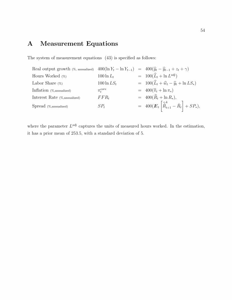
54

A Measurement Equations

The system of measurement equations (43) is specified as follows:

Real output growth (%, annualized) 400(lnYt − lnYt−1) = 400(yt − yt−1 + zt + γ)

Hours Worked (%) 100 lnLt = 100(Lt + lnLadj)

Labor Share (%) 100 lnLSt = 100(Lt + wt − yt + lnLS∗)

Inflation (%,annualized) πcoret = 400(πt + ln π∗)

Interest Rate (%,annualized) FFRt = 400(Rt + lnR∗),

Spread (%,annualized) SPt = 400(IEt

[Rk

t+1 − Rt

]+ SP∗),

where the parameter Ladj captures the units of measured hours worked. In the estimation,

it has a prior mean of 253.5, with a standard deviation of 5.