the gender wage gap within the managerial workforce: an ... · the gender wage gap within the...
TRANSCRIPT

The gender wage gap within the managerial workforce an investigation using Australian
panel data
Ian Watsonlowast
2009 HILDA Survey Research Conference The University of Melbourne
17 July 2009
Abstract
This paper examines the gender pay gap among full-time managers in Australia over the period 2001 to 2007 It finds that women full-time manshyagers earn about 25 per cent less than their male counterparts Decomshyposition methods show that between 70 and 90 per cent of this earnings gap cannot be explained by recourse to a large range of demographic and labour market variables A large part the earnings gap is simply due to women managers being female Despite the characteristics of male and female managers being remarkably similar their earnings outcomes are very different suggesting that discrimination plays a major part The pashyper uses seven waves of HILDA data to fit both OLS and multilevel modshyels to a sample of full-time managers The regression results become the basis for a number of decompositions using a variety of Blinder-Oaxacashystyle methods In addition a recent lsquosimulated changersquo approach develshyoped by Olsen and Walby in the UK is also implemented using this Ausshytralian data
1 Introduction Until the early 1970s the gender wage gap in Australia was wide and was kept that way by lsquoinstitutionalised gender wage discriminationrsquo in the words of Paul Miller (1994 p 371)1 The historic equal pay decisions of 1969 1972 and 1974 ended this and helped close the gap considerably (see for example Gregory and Duncan (1981) Borland (1999)) Nevertheless a gender pay gap of considerable size has remained as Borland noted in his overview at the end
lowastSenior Research Fellow Politics and International Relations Macquarie University Sydney Email ianwatsonmqeduau This paper was originally planned to be a cross-national comshyparison between Germany and Australia but ill health prevented my intended co-author Elke Holste (DIW Berlin) from contributing Her inspiration for suggesting this project is much appreciated The R routine developed for carrying out the decompositions in this paper beneshyfited considerably from Ben Jannrsquos exemplary exposition of his Stata oaxaca routine in the Stata Journal See Jann (2008)
1 This paper uses unit record data from the Household Income and Labour Dynamics in Ausshytralia (HILDA) Survey The HILDA Project was initiated and is funded by the Australian Government Department of Families Housing Community Services and Indigenous Affairs (FaHCSIA) and is managed by the Melbourne Institute of Applied Economic and Social Reshysearch (MIAESR) The findings and views reported in this paper however are those of the author and should not be attributed to either FaHCSIA or the MIAESR
1
of the 1990s He summarised a number of studies which showed estimates for the wage gap during the 1980s and 1990s ranging from about 8 per cent through to about 25 per cent (Borland 1999 p 267) Borland also summarised the lsquodiscriminatory componentrsquo of this gap as ranging from about 7 per cent to about 19 per cent a considerably portion of the actual gap He concluded that most of the reduction in the wage gap since the early 1970s was due to a lsquodecrease in wage discriminationrsquo (Borland 1999 p 268)
The early equal pay cases did not fully pursue the labour market dimension of the gender pay gap particularly occupational-based gender segregation By the 1990s this had become the focus for pay equity inquiries (such as that in NSW) and the concept of comparable worth became central Pocock (1999) Usshying data from the late 1980s Miller (1994) found a gender wage gap of about 13 per cent with a large component of that gap (6 percentage points) due to occushypational concentration As Miller noted lsquoabout 40 of the differential might be removed by the implementation of true comparable worthrsquo (1994 p 367) Usshying a comparable but later data set Wooden (1999) also examined the issue of comparable worth While the actual wage gap was smaller in Woodenrsquos study (115 per cent) his results were broadly similar to Miller rsquos Wooden found that occupational concentration accounted for 42 percentage points that is about one third (1999 p 167)
Wooden however argued that including the managerial workforce in such studies was unwarranted When he removed managers from the sample he found that the gender wage gap fell to 89 per cent with the occupational concentration component now accounting for 36 percentage points Wooden noted that the under-representation of women in senior management positions in Australian companies was likely to widen the gender wage gap because managers earned much more than the all-occupational average As a conseshyquence he concluded this removed the scope for industrial tribunals to elimishynate a considerable part of the gender wage gap because lsquothe earnings of manshyagers typically lie outside the purview of industrial awardsrsquo Wooden further added lsquothe problem is not necessarily one of unequal earnings but rather of unequal access to promotionrsquo (Wooden 1999 p 167) The implications of this argument will be pursued at length in the discussion section of this paper
While much of the research on the gender pay gap has focussed on the workforce more generally or at least the full-time workforce recent studies have begun to examine the gap across the entire wage distribution pursuing the recognition that the gap is not uniform across this distribution Innovashytions in the use of quantile regression methods (for example Buchinsky (1998) Koenker and Hallock (2001)) has opened up this field of research In Australia both Miller (2005) and Kee (2006) have used this approach to explore the genshyder pay gap
Miller found that the wage gap was much greater among high wage earners than among low wage earners
the gender wage gap generally widens as one moves up the wage scale The wage differentials are below 10 per cent from the 5th to the 35th quantile and then the gap increases from 12 percentage points at the 40th quantile to 23 percentage points at the 95th quanshytile (2005 p 412)
This led him to argue lsquowhile the policy debate on the gender wage gap needs to focus on all parts of the wage distribution there is a particular need for
2
attention among high-wage earnersrsquo (2005 p 412) Keersquos study extended Miller rsquos by separately analysing the public and prishy
vate sectors She found that the gender pay gap increased at higher levels in the private sectormdashleading to her conclusion that a lsquoglass ceilingrsquo existed theremdash but that the gap in the public sector was lsquorelatively constantrsquo over all percentiles (Kee 2006 p 424)
In this paper I look more closely at the top of the wages distribution by examining the gender pay gap among full-time managers2 Among this subshypopulation this gap is distinctively larger while at the same time confounders like occupational-based gender segregation and part-timefull-time wage rashytios are largely absent (see for example Whitehouse (2001)) The approach I take implements various classic Blinder-Oxacaca-style decompositions but I also consider a more recent lsquosimulated changersquo approach developed by Wendy Olsen and Sylvia Walby in the UK (Olsen and Walby 2004 Walby and Olsen 2002) This approach is particularly relevant because it allows researchers to examine more closely some of the policy-related dimensions of the gender pay gap
2 The decomposition of wage differentials 21 The Blinder-Oaxaca tradition
The use of Blinder-Oaxaca-style decompositions have been a mainstay of soshyciological and economic analysis for the last 35 years Since their pioneering work in the early 1970s the core approach of Blinder (1973) and Oaxaca (1973) has been reproduced many times though with variations and extensions to acshycommodate methodological weaknesses and different assumptions The core technique is quite straightforward After fitting separate regressions for men and women the predicted wage gap is decomposed into that component based on the differing characteristics of each group and another component based on how those characteristics are rewarded in the labour market (the regression coefficients) Only the difference in characteristics can be readily explained and in this sense the unexplained portion of the wage gap can be regarded as discriminatory From within a human capital framework the differences in characteristics have usually been referred to as a difference in lsquoendowmentsrsquo (Blinder 1973) or as a lsquoproductivity differentialrsquo (Oaxaca and Ransom 1994) The unexplained component has been variously referred to as the lsquocoefficients effectrsquo or more generally the lsquodiscriminationrsquo component
While it is common to see the terminology of lsquoendowmentsrsquo and lsquodiscrimishynationrsquo used throughout the literature it is important to keep in mind several caveats around these terms The first term is usually based on human capital assumptions about wages and productivity giving rise to a preference for a more neutral term like lsquocharacteristicsrsquo The term lsquodiscriminationrsquo can be misshyleading within the decomposition method it is only ever identified as a residshyual the part that cannot be explained by the characteristics of the sample In the words of Dolton and Makepeace (1986 p 332) lsquothe residual is really a meashysure of our ignorancersquo In this paper my own preference is to use the terms lsquocharacteristicsrsquo and lsquounexplainedrsquo
2 The terms wages pay and earnings are used interchangeably in this report The analysis foshycuses on annual wage and salary income so the term earnings is probably more accurate than wages (which implies an hourly rate) but the relevant literature generally uses the terms lsquopay gaprsquo and lsquowages gaprsquo
3
The core decomposition approach can be illustrated as follows The wage gap between the two groups can be viewed as the difference in the predicted means of the (natural) logs of male (m) and female ( f ) wages and following the fitting of separate regression functions it can be represented by
macrwm minus w f = Σβm Xm minus Σβ f X f (1) macrwhere the βs are the regression coefficients and the Xs are the vectors of mean
characteristics Re-arranging the terms and representing the wage gap by Gm f it is straightforward to show that there are at least two ways of decomposing this wage gap
macrGm f = Σβ f (Xm minus Xf ) + ΣXm(βm minus β f ) (2)
macrGm f = Σβm(Xm minus Xf ) + ΣX f (βm minus β f ) (3)
In each case the first part of the right-hand sides of these equations contain estimates of the differences in the characteristics of males and females weighted by the female (2) and male (3) coefficients In other words the differences in the characteristics of each group are rewarded according to the wage structure of females or males (depending on which decomposition is used) The second set of terms in these equations capture the lsquodiscriminationrsquo component they measure the differences in each wage structuremdashhow the labour market differshyentially rewards each groupmdashapplied to the male (2) and female characteristics respectively (3) (See Neumark (1988 p 281) and Cotton (1988 p 236))
It is clear from these two equations that a key choice within the decomposishytion approach is deciding what constitutes the non-discriminatory benchmark against which to weight the differences Regarding the female wage structure as non-discriminatory leads to a lsquoprivilege modelrsquo of discrimination in that males earn more than they should in a non-discriminatory world On the other hand regarding the male wage structure as the norm leads to a lsquodeprivation modelrsquo in which females earn less than they would in a non-discriminatory world (Jones and Kelley 1984 p 331)3
Lying behind these equations are different assumptions about the operashytions of the labour market In the case of equation (2) males earn an unshydeserved premium in the labour market and an absence of discrimination would see the female wage structure applied uniformly across the labour marshyket In the case of equation (3) females are penalised in the labour market and ending discrimination would see the rate of return on their characterisshytics come to match that of the male wage structure In either case a nonshydiscriminatory wage structure would result in a wages gap which reflected only (non-discriminatory) differences in characteristics
Much of the literature subsequent to the early work of Blinder and Oaxshyaca has concentrated on examining different non-discriminatory benchmarks These have gone beyond equating non-discrimination with either the male or female wage structure Reimers (1983 p 573) for example suggested that in lsquonon discriminatory worldrsquo the wage structure by which to weight the differshyences would most likely lie somewhere in between Cotton (1988 p 238) in the context of racially based wage gaps took a similar view
3 Jones and Kelley present their decomposition with an lsquointeraction termrsquo which they define as Σ(βm minus β f )( Xm minus X f ) They note that the deprivation model allocates this interaction term to macrthe unexplained differences component while the privilege model allocates it to the charactershyistics component (1984 p 331)
4
not only is the group discriminated against undervalued but the preshyferred group is overvalued and the undervaluation of the one subsidizes the overvaluation of the other Thus the white and black wage structures are both functions of discrimination and we would not expect either to prevail in the absence of discrimination
Where Reimers took the average difference between the male and female wage structures Cotton weighted the white and black wage structures by the proportions of each group in the labour force (1988 p 239) Neumark (1988) reshygarded these benchmarks as unsatisfactory and argued that the choice of a nonshydiscriminatory wage structure should be based on theoretical grounds Using Beckersrsquo theory of employer discrimination (Becker 1971) Neumark derived an lsquoestimable no-discrimination wage structurersquo (1988 p 283) which he used as his weighting scheme In a similar fashion Oaxaca and Ransom (1994 p 9) criticised both Reimers and Cotton for adopting a non-discriminatory wage structure which was basically lsquoarbitraryrsquo Like Neumark they proposed as their non-discriminatory wage structure a weighting matrix based on the OLS estishymates from a pooled regression (of both males and females) arguing that these pooled estimates reflected lsquothe wage structure that would exist in the absence of discriminationrsquo (1994 p 11)
These approaches are summarised in Table 1 which draws upon the preshysentation of results developed by Oaxaca and Ransom (1994 p 13) It is useshyful because it makes the non-discriminatory benchmark explicit and it also shows that the unexplained or lsquodiscriminatoryrsquo component can be further deshycomposed
macrGm f = Σβ lowast(Xm minus Xf ) + ΣXw(βm minus β lowast) + ΣX f (β lowast minus β f ) (4)
Here β lowast makes explicit the non-discriminatory wage structure As before the first term on the right-hand side shows the differences in male and female characteristics weighted by a particular wage structure in this case the nonshydiscriminatory benchmark β lowast The second and third terms represent the last part of equations (2) and (3) in which the unexplained component is now deshycomposed into that part which reflects male privilege and that part which reshyflects female disadvantage The last two columns in Table 1 show the weighting matrix which is applied in each of the approaches listed The diagonals of this matrix consist of either 1s or 0s (identity matrix and the null matrix) in the first two approaches a set of ratios (05 and the female-male ratio) in the Reimers and Cotton approaches and a set of weights based on the differences between the pooled regression coefficients and the separate male and female regression coefficients (the Neumark and Oaxaca and Ransom approaches)
5
Table 1 Decomposing wage gaps conceptual framework
Unexplained (lsquodiscriminationrsquo) decomposed into
Approach Non-discriminatory benchmark
Male advantage
Female disadvantage
Deprivation Privilege Reimers Cotton Pooled
Male Female
Male-female average Female-male ratio
Pooled coefficients ( p)
0 I
05 f m
m minus p
I 0
05 1 minus f m
p minus f
Note There is actually no further decomposition in the privilege and deprivation models (since the null matrix removes the non-applicable term) but they are shown in this table in this way so that all approaches can be compared within the one framework Source Based on Oaxaca and Ransom (1994 p 13)
As well as the tradition outlined here other decomposition approaches have been taken within labour economics Another popular strategy has been to implement a Juhn-Murphy-Pierce decomposition (see Juhn et al (1991)) but as Neuman and Oaxaca (2004 p 3ndash4) argue the estimation results using JMP decomposition are largely the same as those produced by using the pooled apshyproach developed by Oaxaca and Ransom (1994) and shown in Table 1 above
Which of the approaches shown in Table 1 used be used for analysing the gender pay gap among managers One might argue that if the focus were those workers at the bottom of the wage distribution then a principle of lsquoequalizing upwardsrsquo (Supiot 2009 p 62) should apply and a deprivation model approach would be appropriate Given that managers occupy the opposite nichemdashat the top of the wage distributionmdashthen a privilege model is probably more approshypriate and the interests of social justice would favour an lsquoequalizing downshywardsrsquo principle
There framework outlined in Table 1 does not utilise a detailed breakdown of the unexplained component neither for individual variables nor for the intercept The earliest decomposition formulations such as Oaxaca (1973) presented detailed results and also separated the intercept regarding it as a lsquogroup membershiprsquo component However it soon became apparent that such an approach was subject to an identification problem As early as 1984 Jones and Kelley (1984 pp 334ndash337) noted that the use of continuous variables which did not have a lsquonaturalrsquo zero point and the use of categorical variables could produce arbitrary results In particular recoding a dummy variable to have a different omitted category could change the relative contributions of the intershycept and the other terms in the unexplained component Oaxaca and Ransom (1999 pp 154) showed that this identification problem also bedevilled attempts to isolate the separate contributions of any of the dummy variables within the unexplained component They did however show that this problem did not apply to the summed terms of the unexplained component (as set out in Table 1 above) Until recently this identification problem has left attempts at detailed decompositions in something of a limbo As Yun observed
Economists have innocently ignored the identification problem when applying decomposition analysis empirically or have simply given up the detailed decomposition of the coefficients effect (2005 p 771)
Yun herself provides one solution as do Gardeazabal and Ugidos (2004 p 1035) use a normalized equation and employ the mean characteristics of
6
each categorical variable Yun does this through a restricted least-squares estishymation approach (2005 p 771) while Gardeazabal and Ugidos (2004 p 1035) achieve the same goal by restricting the coefficients to sum to zero that is through a transformation of the dummy variables In practice this amounts to using so-called deviation contrast coding (also called lsquoeffect codingrsquo) such that for any particular categorical variable the coefficient of each category reflects a deviation from the grand mean This is the approach adopted in this paper for producing the detailed decomposition tables shown below4
22 A simulated change approach
As noted earlier the Blinder-Oaxaca approach is not the only way to decomshypose the gender pay gap A recent innovation developed by Sylvia Walby and Wendy Olsen in the UK (Walby and Olsen 2002 Olsen and Walby 2004) has emphasised the importance of pooled regressions rather than the separate reshygressions which are at the core of many of the traditional methods5 As they argue lsquousing separate regressions for women and men implies untenable asshysumptions as to the separation of male and female labour marketsrsquo (Olsen and Walby 2004 p 5) In the case of managers this argument has considerable purshychase particularly given the similar profiles which male and female managers exhibit (with the exception of their industry distinctiveness)
The approach developed by Olsen and Walby (Olsen and Walby 2004 pp 63ndash70) entails fitting a pooled regression and then using simulated changes in the characteristics of the sample to quantify the contribution made by gender to the actual wages gap In practices one multiplies the (pooled) model coeffishycients by the gender difference in the mean values for each of the variables in the model This can be represented by
wm minus w f = sum βΔX (5)
where ΔX represents the difference in two means ( xm minus x f ) for each variable In the case of dummy variablesmdashsuch as gender itselfmdashthe difference represhysents a switch from one category to another (eg male to female) Olsen and Walby term ΔX a lsquochange factor rsquo and by multiplying it by β they calculate a lsquosimulation effectrsquo (that is βΔX) This simulation effect can be expressed as a percentage of the pay gap and also conveniently as a monetary equivalent of the actual pay gap (Glancing forward to Table 11 may make this exposition clearer)
Olsen and Walby note that their approach is similar to using standardised regression coefficients but without the incoherent treatment of binary variables entailed in that method Instead
an explicit simulation in which is variable is treated substantively and is examined to see how far a reasonable hypothetical change would affect the outcome is even better than beta coefficients (Olsen and Walby 2004 p 69)
4 Note that all the regression results shown in the appendix use the more conventional treatment contrast coding since the interpretation of dichotomous dummy variables is more straightforshyward (for example the coefficient is a simple contrast with the omitted category rather than a contrast with the average between the two)
5 With the exception of Oaxaca and Ransom (1994) Neumark (1988) who also used pooled reshygressions as shown in the last row of Table 1
7
One can apply this approach to all of the variables in the regression or to just a subset Olsen and Walby for example argue that some variables should just be regarded as controls (such as region or industry) while others are reshygarded as having more policy relevance (such as working hours or education) By hypothesising a change in the latter the researcher can examine those facshytors which influence the wages gap and which are amenable to policy initiashytives In practice this approach makes it possible to estimate the change in earnings lsquothat would occur if womenrsquos conditions changed to reflect the best or the average situation among menrsquo(Olsen and Walby 2004 p 66) In this respect they come closer to the assumptions of the lsquodeprivationrsquo approach disshycussed earlier
As an example one can examine the simulation effect of any particular variablemdashsuch as years of part-time workmdashand express this as a percentage of the pay gap Using British Household Panel Survey data Olsen and Walby (2004 p 65) find that this particular variable has a simulation effect of 002 which accounts for 10 per cent of the gross wages gap of 023 This variable can then be given a monetary value namely 24 pence per hour (10 per cent of the pound228 wages gap) In the final section of this paper I implement the OlsenWalby approach and illustrate its relevance in the Australian setting
3 Modelling issues 31 Sample selection bias
The sample of persons under scrutiny in this paper are only a subset of all pershysons contained in the HILDA survey dataset Only employees working as full-time managers are included in the modelling dataset and these exclusions have important implications for fitting earnings equations The modelling must deal with problems of sample selection bias that fact that only a subset of individshyuals are observed within this category of interest and only some of these are observed in all years If such selectivity were purely random this would not be an issue but the factors which influence selection into the sample may to be correlated with the regressors which predict the outcome of interest namely earnings If such factors are observable then they can be included in the reshygression model and bias in the estimates can be overcome However the possishybility that unobservable factors influence selection into the sample remains an obstacle A large literature has evolved devoted to this problem (see for examshyple the overview in Vella (1998)) The issue is particularly pertinent to studies of womenrsquos wages given the labour force participation decisions entailed (see for early examples Dolton and Makepeace (1986) Bloom and Killingsworth (1982)) Sample selection bias was also an obvious issue confronted at an early stage in the decomposition literature (for example Reimers (1983))
It is important to be clear about what is at stake In much of the literature on sample selection illustrated by womenrsquos wages the issue is one of being able to generalise to what all women would earn when we only observe a subset of them actually working However in the case of this study we are not seeking to generalise to a larger group of which managers are a subset Rather managers are the population of interest and the sample is a sample of managers6 Despite this difference the underlying predicament of selection bias remains it is still the case that some unobservable factors may influence both who becomes a
6 Though it could be argued that the exclusion of part-timers makes this a comparable analogy but for practical purposes the numbers involved are very small
8
manager and what they are paid In this respect the necessity to correct for sample selection among managers is as important for males as for females7
While maximum likelihood estimators are often used to model both seshylection and earning equations simultaneously in this study I make use of the Heckman two-step approach (Heckman 1979) It has a number of advantages when it comes to more complex models such as multilevel models not least its computational simplicity The most common selection models are binarymdash working or not workingmdashand are fit using probit regression In this case the potential outcome is threefoldmdashworking as a full-time manager not working as a manager or not working at all and a multinomial logit model is more apshypropriate (see for example Rodgers (2002)) The following selection equation for individual i in each group j (males and females) takes the form
Pr(Yi j = 0) = γ
1 + ti j (6)
1 Zi j + eγ2 Zi j 1 + e
γ e k Zi j
Pr(Yi j = k) = γ
+ ti j k = 1 2 Zi j + eγ2
Zi j 1 + e k
ti j sim N(0 1)
where k = 0 1 2 for not working at all working and working as a full-time manager respectively ti j is the usual error term and Z represents a matrix of characteristics likely to influence whether an individual is observed in the parshyticular category of interest The details of the variables used in this model are discussed below suffice it to note that after running this model separately for each group (that is males and females) the inverse of Mills ratio (for working as a full-time manager) is calculated for each observation in the sample and this term is then incorporated into the earnings equation in the second stage as a lsquocorrectionrsquo term8
The main equationmdashthe OLS earnings equation which is also fitted sepashyrately for males and femalesmdashtakes the classic form
ln Wi j = Xi j β j + cjλi j + t2i j (7)
where t2i j sim N(0 σ)
corr(ti j t2i j ) = ρ
and where ln Wi j is the (log) of the annual earnings for each individual i in each group j The term X is a matrix of relevant demographic and labour market explanatory variables λ is the correction term for the selection effect and t is the usual error term If the error term for the earnings equation (t2i j ) and the error term for the selection equation (ti j ) are correlated (if ρ = 0) then a
7 For example in some labour-market wide studies the correcting for sample selection bias is only applied to women workers
8 For details on the construction of the inverse of Mills ratio see Cameron and Trivedi (2005 p 550) For its construction following multinomial logit see Rodgers (2002 p 235) Hamilton and Nickerson (2001 pp 38ndash39) To ensure identification without relying on the functional form variables related to the presence of young children (which were not included in the earnshyings model) were included in the multinomial logit model The full details are discussed later in the paper
9
lsquoselection effectrsquo would appear to be operating This can be tested with a Wald test on the coefficient cj in the earnings equation A statistically significant result endorses the presence of a selection effect
This approach is useful because it lsquocorrectsrsquo the coefficients in the earnings equation for the effect of selection bias and in that respect plays an important role Where the debate lies from the point of view of the decomposition literashyture is where to assign the selection effect itself within the final decomposition The selection effect takes the following form
macr macr cmλm minus c f λ f (8)
where m refers to males and f to females Reimers (1983) for example reshygarded (8) as a separate category from the characteristics and discrimination effects and proceeded to decompose an lsquoadjusted wage gaprsquo that is the wage gap which had been corrected for selection bias Nevertheless as Neuman and Oaxaca (2004) observe where to assign the selection effect is a complex issue involving a range of assumptions about how discrimination operates in the labour market They note that the Reimersrsquo approach is lsquononcommitalrsquo about whether to assign this term to characteristics or discrimination and it avoids some of the identification problems which can arise if one tries to assign the term in a more unequivocal fashion (2004 p 8) As will be discussed below I find that the selection effect is not statistically significant so the decomposishytions carried out for this paper do not deal with this issue
32 Panel data and multilevel modelling
There are a number of advantages in using panel data for this study Because the category of interest is such a small groupmdashfull-time adult managersmdash sample size considerations are paramount There are major gains in the precishysion of the estimates for the decomposition results from using a larger number of observations from pooling the data across all waves Moreover the use of multilevel modelling (also called mixed-effects modelling) with panel data also provides a correction to the coefficients
Using a multilevel modelling strategy (see Pinheiro and Bates (2004) and Gelman and Hill (2007) for the approach taken in this paper) entails fitting a model with a fixed componentmdashthe usual set of earnings regression controlsmdash as well a random component The actual dataset observations can be regarded as lsquoearnings episodesrsquo which are clustered within individuals who themselves are clustered within households On the one hand this hierarchical data strucshyture poses challenges for calculating standard errorsmdashbecause of the violation of the iid assumptionmdashbut it also offers distinct advantages Multilevel modshyelling provides a kind of lsquopartial poolingrsquo of the data In this respect it avoids the pitfalls of complete poolingmdashwhich would lead us to ignore differences between individuals and suppress variation in the datamdashand on the other hand no pooling with its problems of unreliable estimates (Gelman and Hill 2007 pp 7 256) One can of course fit a fixed-effects model to panel data but a particular advantage of the multilevel approach is its ability to make use of sparse observations Because the population of interest is small the loss of every observation matters A fixed-effects approach requires at least two obsershyvations on the same individual across the panel whereas a multilevel approach can suffice when there is only one observation (Gelman and Hill 2007 p 276) In the case of the HILDA panel of managers used in this study there are a large
10
number of individuals (44 per cent) who only appear once in the panel with females more likely to be in this situation (48 per cent) than males (41 per cent) Their omission does not just reflect absence from the labour market but occushypational mobility and the fact that becoming a manager is a step some distance along the career pathway
The coefficients for the fixed-effects from the multilevel model are used as the basis for the decomposition of the earnings gap The error terms from the model can also be decomposed into their appropriate levelsmdashepisode individshyual and householdmdashfor additional insights into the sources of earnings varishyability
For the multilevel modelling the earnings equation takes the form
ln Wi jt = Xi jt β jt + cjtλi jt + ti jt (9)
where ln Wi jt is the (log) the annual earnings for each individual i in each group j in period t The term Xi jt is a matrix of relevant demographic and labour market explanatory variables cjt λi jt is the correction term for the selecshytion effect as discussed earlier and ti jt is the usual error term The iid assumpshytion regarding this error term is violated since the model contains repeated observations for the same individual
In practice the inverse of Millsrsquo ratio is calculated for each wave of the data and then incorporated into the pooled dataset Equation (9) is then fitted to this dataset using the specification required by a multilevel approach for varying intercepts (more details on this are provided below)
4 Data and descriptive overview This paper draws on the Australian GovernmentMelbourne Institutersquos Houseshyhold Income and Labour Dynamics in Australia Survey (HILDA) This is an onshygoing longitudinal survey of Australian households which began in 2001 and which is representative of the Australian population9 The data for this paper comes from Release 70 The descriptive data and the single wave models come from Wave 7 (2007) While this descriptive data uses cross-sectional reshyspondent weights the panel models are unweighted and make use of unbalshyanced panels
There are two possibilities in choosing a sample of managers all adult emshyployees and all adult full-time employees (the choice of employee and adult is axiomatic if one wants to focus on labour market earnings without the complishycations of self-employment and junior rates of pay) Managerial occupations are one of the few occupational groups where most employees do work as full-timers among males the percentage is 96 per cent and females it is 83 per cent By way of comparison the all-occupational percentages are respectively 87 per cent for males and 57 per cent for females
The differing profiles of all managers and full-time managers are shown in Table 2 and there are several notable features of the data The profile of female full-time managers differs little from that of all female managers except for marital statusmdashthe former are more likely to be singlemdashand organisational sizemdashthe former are more likely to be in smaller organisations
9 For more information on the HILDA survey see the HILDA Survey User Manual (Watson 2008)
11
Table 2 Overview of characteristics of managers Australia 2007 ()
All personsdagger Full-timersDagger
Female Male Total Female Male Total
Age group Aged 21-24 7 6 7 8 4 7 Aged 25-29 8 9 10 9 9 10 Aged 30-34 22 15 16 20 15 16 Aged 35-39 16 17 17 16 18 17 Aged 40-44 11 13 12 11 14 12 Aged 45-49 14 11 15 13 11 15 Aged 50-54 11 12 11 12 12 12 Aged 55 or above 11 17 13 10 16 12
Education Uni 36 34 38 39 35 40 Vocational 29 37 33 27 37 33 Year 12 16 16 14 18 15 14 Year 11 or below 19 13 14 17 13 14
Marital status Couple 72 79 77 69 80 77 Single 28 21 23 31 20 23
Industry Primary industry 2 7 6 1 7 6 Manufacturing 3 18 12 4 19 13 Utilities 1 1 1 1 1 1 Construction 0 5 4 0 5 4 Wholesale 2 8 4 3 8 4 Retail 19 12 15 18 12 15 Accommodation cafes etc 9 4 6 7 4 5 Transport 1 2 2 0 3 2 Information services 3 3 3 3 3 3 Finance amp insurance 10 8 7 10 8 8 Business services 14 13 12 14 12 12 Government 10 9 9 11 10 10 Education 9 5 7 8 5 7 Health amp community 12 3 7 12 3 7 Other services 5 1 3 6 1 3
Sector Private 77 85 82 75 86 81 Public 23 15 18 25 14 19
Organisational size Under 20 17 22 20 11 21 17 20 to 99 14 14 12 16 14 13 100 to 499 16 18 19 18 18 19 500 plus 53 46 49 56 47 51
Hours status Full-time 83 96 92 100 100 100 Part-time 17 4 8 0 0 0
Sample size 226 391 627 190 377 573
Notes Weighted data (weighted by cross-sectional weights) Source Unit record data HILDA Release 7 Population Wave 7 2007 dagger All adult respondents working as employees and in management occupations Dagger All adult respondents working as employees in management occupations and working 35 hours or more per week
12
Figure 1 Profile of full-time managers 2007
(Source as for Table 2)
0 5 10 15 20 25 30 35
Occupational tenure
Years in occupation
FemaleMaleCommon
0 5 10 15 20 25 30 35
Job tenure
Years in current job
20 30 40 50 60 70
Age
Age
10 12 14 16 18 20
Years of education
Years of education
20 40 60 80 100
Occupational status
Status score
10 20 30 40 50 60 70
Hours worked
Hours per week
13
On the other hand the differences between male and female full-time manshyagers are more pronounced Compared with their male counterparts female managers are younger are less likely to have vocational qualifications are more likely to be single are more likely to work in the public sector and are more likely to work in larger organisations Their industry profiles are also distinct compared to male managers females are less likely to be found in manufacturing and much more likely to be found in health and community services
Some of the other characteristics of male and female full-time managers are shown in Figure 1 which also emphasises these differences These graphs show kernel density distributions for a number of continuous variables with male (blue plus mauve) and female (orange plus mauve) distributions overlaid This allows one to see where the distributions are common (mauve) and where they are distinctive (blue and orange respectively) Male means are shown as a solid line females means as a dashed line Compared to the male managers females have less occupational and job tenure and are more likely to cluster at the lower end of the full-time hours distribution In terms of years of education and occupational status scores their profiles are reasonably close
What is most striking about the comparison between male and female manshyagers is their similarity Apart from industry location and the public sector private sector split they really are quite comparable Indeed much more so than would be the case with an all-occupational comparison
These differences in the characteristics of male and female managers are one of the key reasons that their earnings differ One of the aims of this paper is of course to decompose how much of the gender earnings gap can be explained by these differing characteristics10
As to the gap pay gap itself its size depends on what is being measured and where it is being measured As Table 3 shows using hourly rates of pay produces a much smaller gap (14 per cent) compared with annual salaries (25 per cent) Moreover the pay gap is greater at the top of the distribution but only mildly so for hourly rates of pay (13 to 15 per cent variation between first and third quartile) With annual salaries this pay gap varies from 15 per cent to 24 per cent between the first and third quartiles The highly skewed nature of these distributions is also notable and is illustrated in Figure 2 which again uses kernel density distributions in the same fashion as described earlier
A likely reason for the lower hourly wages gap is the difference in hours worked between male and female full-time managers The former work on average 48 hours per week the latter 457 Because the hourly rate is based on a simple arithmetic division of weekly wage divided by usual hours the obvious effect of working longer hours is a reduction in the hourly wage meashysure Thus longer hours by males results in a lower hourly rate for them and a consequent reduction in the gender gap In reality managerial jobs are rarely paid on an hourly basis and the hours requirements are usually open-ended so it makes little sense to pursue an analysis based on hourly rates However to make earnings comparable between males and females the sample needs to be restricted to full-timers Fortunately as we have just seen the profile of part-timers and full-timers differs little and the number of lost observations is also minimal To make for greater comparability all of the models discussed
10 In this descriptive section the familiar term lsquogaprsquo is used and the measure is either dollars or percentage points In the modelling section below the term lsquodifferentialrsquo is used and it refers to the difference in log annual wage and salary income (or earnings)
14
below include a control for weeks worked in the year to take account of the likely gender differences in annualised labour force participation
Table 3 Earnings gap hourly rates and annual salaries (all and full-timers)
All (hourly rate $) Full-timers (annual salary $)
Mean 1st Qu Median 3rd Qu Mean 1st Qu Median 3rd Qu
Male Female Gap
34 29 5
21 18 3
28 24 4
40 34 6
87800 65900 21900
52000 44400 7600
71000 62000 9000
106000 81000 25000
Gap () 14 13 13 15 25 15 13 24
Notes Weighted data Source Unit record data HILDA Release 7 Population Adult respondents working as employees and in management occupations all (n = 617) and full-timers (n = 567)
Figure 2 Earnings distributions hourly rates and annual salary 2007
(Source As for Table 3)
Hourly rates (all)
Hourly rates ($)
0 10 20 30 40 50 60 70 80 90
FemaleMaleCommon
Annual salary (fullminustimers)
0 50 100 150 200 250
Annual salary ($000s)
The size of the gender pay gap shown here is what one would expect given earlier research In his analysis of the full-time workforce using 2001 Census data Miller found that the gender pay gap at the 95th percentile was about 23 percentage points The equivalent figure from the HILDA dataset (Wave 7) for all occupations is 25 percentage points11 Given that most managers are likely to be found in vicinity of the 95th percentile one would expect that the size of the gap among the managerial workforce will be of this order of magnitude While not directly comparablemdashbecause of her publicprivate sector splitmdash Keersquos quantile analysis of the HILDA data also found comparable results She found a differential (in log wages) at the 90th percentile of about 027 for the private sector and 012 for the public sector Kee (2006 p 416)
11 The age restriction is greater in Miller rsquos dataset 20 to 64 compared to 21 and over here Miller uses the full-time workforce this figure is based on all full-time employees
15
5 Results 51 Regression modelling
Description and summaries for the variables used for these models can be found in the appendix as Tables 13 and 14 The main variation in the codshying of these variables is the use of a lsquoblue collar rsquo industry grouping This comprises a range of industries where women managers are seldom foundmdash manufacturing mining utilities wholesale and transportmdashand is a necessary aggregation to deal with sparse observations
The modelling strategy in this paper involved increasing the complexity of the models by moving from OLS to multilevel models and then to selectivity-corrected multilevel models Models are fit separately for males and females and interest centres on the earnings differential between males and females and how this might be decomposed in various ways In order to allow for a lsquopooledrsquo decompositionmdashthe Oaxaca and Ransom (1994) approachmdashand in orshyder to implement the Olsen-Walby approach a model using pooled male and female data is also fit Following Jann (2008 pp 457ndash458) a dummy for sex was included in the pooled sample to avoid possible distortion of the decomshyposition results
Before discussing the results of the earnings models it is worth briefly sumshymarising the results of the selection models using the results of the 2007 data for illustration12 As noted earlier these were multinomial logit models with three possible outcomes working as a full-time manager working otherwise or not working at all The predictors in this model were age years of educashytion marital status number of children aged 0 to 4 number of children aged 5 to 9 and whether city or non-city resident The model was run for males and females and the inverse of Mills ratio was calculated for each person in each wave to provide a Heckman correction term (λ) for use in the final multishylevel model The multinomial model results for the 2007 data are shown in the appendix as Table 15
The results of these models are consistent with expectations The selection model for males shows that the likelihood of entering management increases with age peaking in the middle years before dropping off in the later years of life Years of education is also positively associated with becoming a manager Marriage (or de facto status) also has a strong association being in this situshyation (compared with being single) increases menrsquos odds of being a manager by a factor of 38 On the other hand the presence of young children slightly reduces a manrsquos odds of entering management (though the results are only statistically significant for children aged 0 to 4)
The female selection model shows that age is also positively associated with entering management as is marriage (or defacto status) Similarly the numshyber of years of education is also positively associated with female entry into management On the other hand the presence of young children has strong negative associations Compared with a woman with no children aged 0 to 4 someone with one child in that age group has only about one quarter the odds of becoming a manager If they have two children in that age group the odds shrink to about one eighth If the children are somewhat oldermdashin the 5 to 9 age groupmdashthe odds improve but only slightly For one child it is just under
12 The multinomial logit model was fitted separately to each year of data but the example given in the appendix is for the latest wave 2007
16
one third and for two children it is about one fifth These results are interesting in their own right and I return to them more
fully in the final discussion It is worth noting at this stage what these findings mean in terms of probabilities Becoming a manager overall is about twice as likely for a man as a woman The HILDA data allows us to quantify this over time For example the unconditional probability of someone in 2001 being a manager in 200713 is about 17 per cent for men and 9 per cent for women If their status in 2001 was not in the labour force the respective figures are 11 per cent and 4 per cent If employed in 2001 then the figures are 20 per cent and 12 per cent
To illustrate the impact of parenting the predicted probabilities from the 2007 model can be calculated14 If a man has no children then his predicted probability of being a manager is 15 per cent If he has two children one of them aged 0 to 4 the other aged 5 to 9 this predicted probability barely changes rising slightly to 18 per cent For a woman with the same charactershyistics the predicted probability for being a manager is she has no children is 11 per cent and this falls to 4 per cent if she has two children in these age groups
Turning now the core modellingmdashthe earnings equationsmdashI discuss them in increasing order of complexity The simplest modelmdashthe OLS model for annual wagesmdashused 2007 data with the dependent variable the log of annual wage and salary income Controls consisted of age marital status number of weeks working in that year state whether city or non-city residence years of education occupational tenure job tenure occupational status usual hours worked union membership status industry sector organisational size single or multiple workplace organisation One of the main issues in this research is occupational comparability not all managers are doing the same kind of work The ANZSCO category of lsquoManager rsquo includes both skill levels 1 and 2 (ABS 12210 p 14) and the gender mix here could be quite crucial to the size of the gender pay gap The inclusion of a variable for occupational status scoremdashwhich is based on a finer level of occupational disaggregationmdashcontrols for some this15 There remains however an issue of how one might control for seniority apart from age I return to this issue in the discussion section below As for age its likely non-linearity was captured by fitting this variable as a grouped categorical variable rather than a quadratic since interest lay in particular age groupings The sample was restricted to adults working full-time and classified as managers in the ANZSCO framework This model was run for males females and a pooled sample with the latter required for the lsquopooledrsquo version of the decomposition The detailed results of this modelling are shown in the appendix as Table 16
The male OLS models for the 2007 data suggests that age is non-linear with earnings for male managers rising to a peak in the 35 to 39 age group Being married (or defacto) brings an earnings premium of about 17 per cent16 Years
13 For this example the outcome is simply a manager with full-time status and employee status ignored
14 It is the relative probabilities which matter here not the absolute For prediction the other regressors in the model are set at certain fixed levels and it is the overall combination which determines the absolute probabilities The other regressors were set at married (or defacto) living in a city aged 30 to 34 and 15 years of education
15 The measure of occupational status score is based on AUSEI06 See McMillan et al (2009)
16 Percentages for categorical variables are calculated from their coefficient x using the formula
17
of education are rewarded well among men with each additional year of study increasing their earnings by 52 per cent Some of the industry differences are striking men who work as managers in finance and insurance earn about 27 per cent more than their counterparts who work in lsquoblue collar rsquo industries An unusual finding is that organisational size does not appear to matter except for male managers in mid-range organisations (100 to 499 employees) This group earn about 20 per cent more than their counterparts in small workplaces
When the 2007 OLS model is rerun with the inclusion of the Heckman corshyrection term (lambda) the magnitude of the coefficients change (as well as their standard errors) but the overall patterns are not dramatically different The Heckman correction term is not however statistically significant suggesting selection bias is not a major issue with this model While the coefficient is quite large the size of the standard error is considerable
The female OLS model suggests that age is close to linearity with little change in the latter years Being married (or defacto) confers no earnings preshymium Each additional year of education is associated with a 39 per cent inshycrease in earnings Organisational size appears to have no association with earnings with none of the coefficients of large magnitude nor statistically sigshynificant The inclusion of the Heckman correction term does not change any of these results in any substantial way The coefficient for lambda is not statistishycally significant
The multilevel models follow the same specification as the OLS models with the addition of two varying-intercept terms individual cross-wave idenshytifier and household identifier These terms along with the usual error term represent the variance components in the multilevel model and can be usefully interpreted as providing insights into the sources of variability in the outcome The detailed results of this modelling are shown in the appendix as Table 17
The differences between the simple OLS and the multilevel model are quite considerable Looking first at the male models it is clear that the effect for age is no longer non-linear but increases steadily right through a male manager rsquos working life Moreover the magnitude of the coefficients for age are larger than in the OLS models As an example a male manager in his early 40s earns about 55 per cent more than a manager in his early 20s By his late 50s this has increased to about 60 per cent more While the earnings premium for male managers in being married (or defacto) remains its effect is much weaker (but still statistically significant) Perhaps the most interesting difference is organshyisational size there is now a statistically significant effect and a linear one working in larger organisations increases a manager rsquos earnings considerably When the same multilevel model is run with the inclusion of a Heckman corshyrection term the overall patterns do not change though there is one notable difference The marriage premium for males in no longer evident The coeffishycient for selection bias is much smaller than was the case in the equivalent OLS model and is now statistically significant (but not strongly so)
Turning now to the female models there are few changes worth noting The linearity in age is still evident with little change in earnings as female managers age The magnitudes of the coefficients are not much larger in the multilevel model than in the OLS By way of example a female manager in her early 40s earns about 30 per cent more than a manager in her early 20s By her late 50s the figure is still just 30 per cent The one change of note is organishy
100 lowast (ex p(x) minus 1)
18
sational size for female managers there is now a statistically significant effect and a linear one with working in larger organisations increasing earnings The inclusion of the Heckman correction term has only one impact it increases the magnitude of the age premium but it does not change its linearity The coefshyficient for selection bias is similar in magnitude to the equivalent OLS model and is weakly statistically significant
The final models the ones used for applying the decompositions differ from the ones just discussed in one respect They include an additional regressormdash the presence of young childrenmdashand they leave out the Heckman correction term This term is removed because it is unlikely to be statistically significant In the case of the OLS models this is clearcut while in the multilevel models the situation is more uncertain The standard errors shown in the appendix are conventional standard errors which take account of the clustered observations but not the two stage estimation method However as the literature shows these standard errors are not accurate in a two-stage estimation and are likely to be an under-estimate This is confirmed when these multilevel models are bootstrapped The standard errors increase substantially and none of the coshyefficients for selection bias come close to statistical significance17 Given that the inclusion of the Heckman selection term has little substantive effect on the coefficients in these models the decision to drop it from the final model is a reasonable one
This decision has the advantage that the presence of children can now be included in the earnings models As mentioned earlier this factor was required for model identification when using the two-stage estimation approach In the earnings models it now takes the form of two variables the presence of chilshydren aged 0 to 4 and the presence of children aged 5 to 9 The full details of both the OLS models and the multilevel models with this specification are shown in the appendix as Table 18
In the male models the presence of children is positive but not statistically significant in the OLS model In the multilevel model the presence of children aged 0 to 4 is statistically significant and moderately positive In the female OLS models the coefficients are both negative and reasonably large for the younger age group But the standard errors are also largemdashno doubt due to the small samplemdashand so the results are not statistically significant On the other hand the multilevel resultsmdashwith their much larger samplemdashproduce statistically significant results for children aged 5 to 9 (though not for children aged 0 to 4) In summary the presence of children aged 5 to 9 is associated with a wages penalty for female managers of about 11 per cent
Finally one of the advantages of a multilevel model with varying-intercepts is the insights it provides into the sources of variability in earnings If we view an observation as an lsquoearnings episodersquo then about one third of the toshytal variability in earnings is due to fluctuations in earnings episodes from year to year A small amount of variabilitymdashabout 12 per centmdashis due to differences between households and the major component of the variabilitymdashabout 56 per centmdashis due to differences between individuals
17 The bootstrap standard errors are not shown in the appendix but are available from the author
19
52 Decomposition results
The decomposition results discussed in this section are based on the models which exclude the Heckman correction term (as just discussed) In the case of the OLS models only summary decomposition results are presented but these are done for 2007 and (in an abbreviated fashion) for the period from 2001 to 2007 In the case of the multilevel models a detailed decomposition is also presented
Looking first at the OLS results Table 4 shows the 2007 results and Table 5 shows those for the period 2001 to 2007 In the case of the former the proporshytion of the gender earnings differential which is unexplainedmdashand potentially due to discriminationmdashvaries from about 33 per cent to about 87 per cent deshypending on onersquos assumptions about the labour market If we adopt the lsquoprivshyilegersquo approach which suggests that male managers earn an unwarranted preshymium by virtue of their gender then the relevant figure is 87 per cent This is also a consistent figure over time as the mean column in Table 5 shows
Table 4 Decomposing earnings gaps OLS results for 2007
Differential due to Unexpl decomp into
Charact- Unexpl- Male Female Unexpl Approach eristics ained advant disadvant as
Deprivation 0137 0067 0000 0067 330 Privilege 0026 0178 0178 0000 872 Reimers 0081 0123 0089 0034 601 Cotton 0100 0104 0059 0045 511 Pooled 0080 0124 -0000 0124 609
Notes Male prediction 11223 female prediction 11019 differential 0204 (All log of annual wage and salary income) Decomposition of OLS models shown in appendix Table 16 Source Unit record data HILDA Release 7 Population Adult respondents working as full-time employees and in management occupations n = 557 (male n = 371 female n = 186)
Table 5 Unexplained as percentage of differential OLS results for 2001-2007
Approach 2001 2002 2003 2004 2005 2006 2007 Mean
Deprivation 597 528 572 539 573 738 330 554 Privilege 746 879 968 722 1078 895 872 880 Reimers 671 704 770 630 826 816 601 717 Cotton 641 635 693 596 735 788 511 657 Pooled 674 643 632 562 672 730 609 646
Notes Based on OLS models for each year with same specification as for 2007 (shown in Table 16) Source Unit record data HILDA Release 7 Population Adult respondents working as full-time employees and in management occupations Waves 1 to 7 2001 to 2007
20
Table 6 Decomposing earnings gaps multilevel model results
Differential due to Unexpl decomp into
Charact- Unexpl- Male Female Unexpl Approach eristics ained advant disadvant as
Deprivation 0087 0187 0000 0187 683 Privilege 0030 0244 0244 0000 892 Reimers 0058 0216 0122 0094 788 Cotton 0069 0205 0076 0129 748 Pooled 0074 0200 0103 0097 731
Notes Male prediction 1118 female prediction 10908 differential 0274 (All log of annual wage and salary income) Decomposition of multilevel models shown in appendix Table 17 Source Unit record data HILDA Release 7 Population Adult respondents working as full-time employees and in management occupations n = 3851 (male n = 2650 female n = 1201) Wave 1 to 7 2001 to 2007
Turning to the multilevel modelmdashwhich pools the data for all years while recognising the hierarchical nature of this datamdashthe decomposition results are shown in Table 6 The figures which measure the unexplained component as a proportion of the differential are also somewhat higher than those figures which were averaged over 2001 to 2007 (shown in Table 5) In the case of the privilege approach this is less so with the figure of 89 per cent shown in Table 6 close to that shown in the OLS results (87 per cent)
The detailed results for the lsquoprivilegersquo approach allow us to pursue this furshyther (see Table 7) This figure of 87 per cent represents 024 out of a total (log) earnings differential of 027 Looking first at characteristics only 03 of the gap is due to differences between male and female managers (evaluated usshying the male wage structure) and most of these differences relate to working fewer hours in the week and fewer weeks in the year On many of the other attributes the differences are negativemdashwhich mean they help close the gapmdash though the magnitudes of these are minimal except for the presence of young children
When it comes to the unexplained component of the wage differential the figures are of larger magnitude The gender differences in coefficients when applied to the characteristics of female managers show that the gap is closed by hours worked and weeks worked (these have negative signs) The differshyences in returns on occupational status scoremdashthe variable which provides a finer measure of managerial categorymdashalso helps close the gap What widens the gap Not very much Those variables with positive signs have quite small magnitudes with differences on coefficients for working in the public sector and being married (or defacto) being the only notable ones So with the coshyefficient differences for most variables helping to close the gender differential why does the unexplained component remain so large at 024 The answer lies in the intercept a figure of considerable magnitude 072 As noted earlier the intercept represents lsquogroup membershiprsquo it is the component of the wage differential which reflects being female rather than male In the earliest decomshyposition studies it was viewed as the most lsquoblatantrsquo measure of discrimination (see for example Blinder (1973))
21
22
Table
7
Det
aile
d d
ecom
position
multile
vel m
odel
res
ults
Dep
riva
tion
Privi
lege
Rei
mer
s Cott
on
Poole
d
Char
act
-U
nex
pl-
Char
act
-U
nex
pl-
Char
act
-U
nex
pl-
Char
act
-U
nex
pl-
Char
act
-U
nex
pl-
Var
iable
s er
istics
ain
ed
eristics
ain
ed
eristics
ain
ed
eristics
ain
ed
eristics
ain
ed
Inte
rcep
t 00
00
07
21
00
00
07
21
00
00
07
44
00
00
07
21
00
00
07
21
A
ge
00
23
-0
004
00
12
00
07
00
17
00
01
00
19
-0
001
00
19
-0
001
Couple
00
09
00
11
-0
002
00
22
00
04
00
16
00
06
00
15
00
05
00
15
Young
child
ren
00
09
-0
093
-0
021
-0
063
-0
004
-0
121
-0
001
-0
084
00
04
-0
089
W
eeks
em
p in
yr
00
09
-0
217
00
11
-0
220
00
10
-0
207
00
10
-0
218
00
11
-0
219
Sta
te
-00
00
-0
005
-0
003
-0
002
-0
002
-0
004
-0
001
-0
004
-0
001
-0
004
N
on-c
ity
resid
-0
003
00
09
-0
002
00
08
-0
002
00
08
-0
002
00
09
-0
002
00
09
Yrs
of ed
uca
tn
00
07
-0
005
00
07
-0
005
00
07
-0
004
00
07
-0
005
00
08
-0
005
O
ccup
ten
ure
00
01
-0
006
00
02
-0
008
00
02
-0
006
00
02
-0
007
00
02
-0
007
Jo
b t
enure
00
03
-0
029
00
09
-0
035
00
06
-0
031
00
05
-0
031
00
05
-0
030
O
ccup
sta
tus
-00
06
-0
144
-0
009
-0
141
-0
007
-0
137
-0
007
-0
143
-0
007
-0
143
U
sual
wkl
y hrs
00
25
-0
071
00
30
-0
076
00
28
-0
070
00
27
-0
073
00
28
-0
073
U
nio
n m
ember
00
01
00
02
00
00
00
02
00
01
00
02
00
01
00
02
00
01
00
02
In
dust
ry
00
08
-0
009
00
02
-0
003
00
05
-0
006
00
06
-0
007
00
06
-0
007
Public
sec
tor
00
07
00
23
-0
003
00
33
00
02
00
28
00
04
00
26
00
03
00
27
O
rgan
isat
siz
e -0
007
00
04
-0
006
00
03
-0
007
00
03
-0
007
00
04
-0
007
00
04
O
rg w
ith
sin
gle
wp
00
00
00
01
00
00
00
01
00
00
00
01
00
00
00
01
00
00
00
01
Tota
l 00
87
01
87
00
30
02
44
00
60
02
15
00
69
02
05
00
74
02
00
Note
s M
ale
pre
dic
tion
111
8 fe
male
pre
dic
tion
109
1 diff
eren
tial
02
7
(All
log
of annual wage
and
sala
ry inco
me
) D
ecom
position
of m
ultilev
el m
odel
ssh
own
in
appen
dix
Table
17
Sourc
e U
nit
rec
ord
data
H
ILD
A Rel
ease
7
Popula
tion
Adult
res
ponden
ts w
orkin
g a
s fu
ll-t
ime
emplo
yees
and
in
managem
ent
occ
upations
n =
38
51
(m
ale
n =
26
50 fe
male
n =
12
01)
One of the key advantages of to using panel data for a study such as this is the increased precision of the estimates Because managers comprise such a relatively small section of the workforce sample size considerations become paramount when drawing inferences from the point estimates In analysing a single wave of data as was done for the simple OLS model the sample size for both male and female managers was just 557 On the other hand using all 7 waves of data provided a sample size of 3850 Valid statistical inference requires some measure of uncertainty in the modelling and the decomposishytion approach in this paper is no exception As Jann (2008 pp 458ndash460) arshygues variability enters the decomposition results through both the variances of the coefficients and the use of random variables from survey sample data Because the decomposition method involves multiplying the coefficients and the means of these random variables one must take account of both sources of variation Following Sinning et al (2008 pp 489ndash90) the approach used in this study involves bootstrapping to obtain standard errors for the final decomposishytion results This approach has advantages when the computation of analytical standard errors is complex and is well suited to panel data models like those employed here (Cameron and Trivedi 2005 p 377)18
The gender wages differential examined in this studymdashof 027mdashhas a stanshydard error of about 002 giving a confidence interval of between 024 and 030 (Table 8) The figures reported earlier in Table 6 are reproduced below in Tashybles 9 and Tables 10 with their standard errors and confidence intervals shown beside them The figure of 89 per cent calculated using the privilege approach has a standard error of 102 percentage points giving a confidence interval of between 67 per cent and 111 per cent Looking across all approaches except the pooled approach this proportion never drops below 52 per cent The pooled approach has a much larger standard errormdashnearly 23 percentage pointsmdashand produces a much wider confidence interval from 28 per cent to 118 per cent
Finally the observation made earlier that differences in characteristics do not explain much of the differential is reinforced by Table 10 We saw earlier that using the privilege approach this figure was 003 Its confidence interval is -003 to 009 With the exception of the pooled approach the highest upper bound figure for characteristics is 013 On the other hand the unexplained component which measured 024 in the privilege approach has a confidence interval of 018 to 031 Again with the exception of the pooled approach the smallest lower bound for this figure never drops below 014
18 Bootstrapping using 1200 repetitions was carried out for the multilevel model using the R routine boot see Canty and Ripley (2009) and Davison and Hinkley (1997) For efficiency the R package snow was used to parallelise the bootstrapping see Tierney Rossini Li and Sevcikova (2009) Tierney Rossini and Li (2009)
23
Table 8 Confidence intervals for gender pay differential
Approach Est SE LB UB
Predicted male 1118 001 1117 1120 Predicted female 1091 001 1088 1094 Differential 027 002 024 030
Notes Est = estimate SE = standard error LB = lower confidence interval bound UB = upper bound 95 confidence intervals Based on bootstrapping the unadjusted multilevel models shown in Table 17 The predicted earnings are shown as the natural log of annual wage and salary income and the differential is also on this scale Source Unit record data HILDA Release 7 Population Adult respondents working as full-time employees and in manageshyment occupations n = 3851 (male n = 2650 female n = 1201)
Table 9 Confidence intervals for Unexplained as percentage of differential (as s)
Approach Est SE LB UB
Deprivation 683 81 525 842 Privilege 892 111 674 1110 Reimers 788 72 647 929 Cotton 748 69 614 883 Pooled 732 230 281 1184
Notes 95 confidence intervals Based on bootstrapping the unadjusted multilevel models shown in Table 17 Source Unit record data HILDA Release 7 Population Adult respondents working as full-time employees and in manageshyment occupations n = 3851 (male n = 2650 female n = 1201)
Table 10 Confidence intervals for characteristics and unexplained components
Characteristics Unexplained
Approach Est SE LB UB Est SE LB UB
Deprivation 0087 0024 0040 0133 0187 0023 0143 0232 Privilege 0030 0030 -0030 0089 0244 0032 0182 0307 Reimers 0058 0020 0018 0098 0216 0021 0174 0257 Cotton 0069 0020 0030 0108 0205 0020 0166 0244 Pooled 0073 0063 -0050 0197 0201 0063 0077 0324
Notes 95 confidence intervals Based on bootstrapping the unadjusted multilevel models shown in Table 17 Source Unit record data HILDA Release 7 Population Adult respondents working as full-time employees and in management occupations n = 3851 (male n = 2650 female n = 1201)
24
53 Simulated change results
In the Olsen-Walby approach the emphasis is on simulated change and its consequences for closing the gender pay gap By hypothesising various changesmdashsome of which may have policy relevancemdashone can estimate how much the gap would close in percentage terms and how much this would be worth to women in dollar terms
Looking first at Table 11 which is based on the pooled version of the 2007 OLS regression it is notable that usual weekly hours is prominent The differshyence between male and female managers in this respect accounts for 21 per cent of the wages gap Were women managers as a group to increase their weekly hours to match the male averagemdasha change of 29 hoursmdashthen this would be worth an additional $4732 per annum Similarly if they increased their avershyage for the weeks employed in the year to match menrsquos then this would reduce the wages gap by about 7 per cent and be worth $1463 per annum
Some of these hypothesised changes have little policy relevance For examshyple it was noted earlier that marriage (or defacto status) confers an advantage on male managers If female managers were to match their male counterparts in this regardmdashsomething requiring a 17 percentage point increasemdashthen this would reduce the wages gap by 7 per cent and be worth $1520 to them
On the other hand the policy relevance of some hypothesised changes is quite clear For example if the representation of women in the ranks of older managers was the same as that of menmdashsomething requiring just under a 5 percentage point increasemdashthen the gender pay gap would shrink by 8 percent and be worth $1755 per annum
Ultimately however it is the intercept term which proves most resistant to policy interventions Simply being a woman accounts for 61 percent of the wages gap If the hypothesised change saw female managers become male managers overnight then this lsquosex changersquo would be worth $13516 to them
The simulated change results for the multilevel model again using the pooled version are shown in Table 12 These largely follow those just disshycussed but the magnitudes differ quite considerably The multilevel model attributes much more of the wages gap to the interceptmdashabout 73 per centmdash and less to changes in usually weekly hours (10 per cent) or weeks employed in the year (4 per cent) Interestingly it highlights an age effect which is less evident in Table 11 Not only is the under-representation of women in the 55 and older age group a liabilitymdashworth about $1179mdashbut so is their under-representation in their middle years If they achieved the same presence in the managerial workforce as men in the 40 to 44 year age range then this would be worth an additional $1147 per annum
While the OLS results suggest a simulated change in marital status is worth about $1520 the multilevel model only rates this change as worth $442 Neishyther model puts much emphasis on simulated changes in the presence of chilshydren the OLS results value such a change at $676 per annum the multilevel results value it at $355 per annum
25
Table 11 Olsen-Walby simulated change OLS model
ΔX β β ΔX Simul Male Female Change Overall Simul chng as Ann $ avg avg factor coeff effect gap equival
Female 0000 1000 -1000 -0124 0124 0609 13516 Aged 25-29 0100 0091 0008 0127 0001 0005 115 Aged 30-34 0146 0177 -0032 0309 -0010 -0048 -1069 Aged 35-39 0167 0167 0000 0345 0000 0001 17 Aged 40-44 0127 0113 0014 0307 0004 0021 460 Aged 45-49 0154 0145 0008 0350 0003 0015 323 Aged 50-54 0119 0118 0000 0306 0000 0000 11 Aged 55 plus 0137 0091 0046 0350 0016 0079 1755 Couple 0822 0656 0166 0084 0014 0068 1520 Children 0 to 4 0208 0145 0062 0015 0001 0005 105 Children 5 to 9 0213 0065 0148 0035 0005 0026 571 Weeks emp in yr 51881 51043 0838 0016 0013 0066 1463 Vic 0264 0263 0001 -0115 -0000 -0000 -9 Qld 0181 0204 -0024 -0084 0002 0010 217 SA 0070 0048 0022 -0005 -0000 -0001 -13 WA amp NT 0092 0086 0006 0009 0000 0000 5 Tas amp ACT 0065 0059 0006 -0097 -0001 -0003 -58 Non-city resid 0342 0296 0047 -0100 -0005 -0023 -509 Yrs of educatn 14493 14339 0155 0039 0006 0029 652 Occup tenure 9841 7769 2072 0005 0010 0049 1094 Job tenure 8272 6981 1292 -0001 -0002 -0008 -170 Occup status 64555 65826 -1272 0011 -0014 -0070 -1550 Usual wkly hrs 48116 45215 2901 0015 0044 0213 4732 Union member 0156 0226 -0069 -0075 0005 0025 565 Retail 0132 0194 -0061 0027 -0002 -0008 -182 Acc cafes rec 0040 0081 -0040 -0012 0000 0002 53 IT amp bus serv 0148 0145 0003 0149 0000 0002 50 Fin amp insurance 0065 0097 -0032 0192 -0006 -0030 -670 Government 0094 0102 -0008 -0010 0000 0000 8 Education 0062 0081 -0019 -0085 0002 0008 173 Health amp community 0046 0204 -0158 -0087 0014 0067 1498 Public sector 0151 0263 -0112 0024 -0003 -0013 -290 Org size 20ndash99 0132 0113 0019 0007 0000 0001 15 Org size 100ndash499 0194 0199 -0005 0161 -0001 -0004 -85 Org size 500 plus 0480 0575 -0095 0149 -0014 -0070 -1546 Org with single wp 0229 0183 0046 -0113 -0005 -0026 -567 Intercept 1000 1000 0000 7961 0000 0000 0 Totals 0204 1000 22200
Notes Based on the pooled 2007 OLS model shown in Table 18 Source Unit record data HILDA Release 7 Population Adult respondents working as full-time employees and in management occupations n = 557 (male n = 371 female n = 186) Wave 7 2007
26
Table 12 Olsen-Walby simulated change multilevel model
ΔX β β ΔX Simul Male Female Change Overall Simul chng as Ann $ avg avg factor coeff effect gap equival
Female 0000 1000 -1000 -0200 0200 0732 16254 Aged 25-29 0093 0137 -0044 0180 -0008 -0029 -643 Aged 30-34 0162 0156 0007 0274 0002 0007 146 Aged 35-39 0164 0135 0029 0337 0010 0036 788 Aged 40-44 0155 0118 0037 0384 0014 0052 1147 Aged 45-49 0140 0172 -0032 0381 -0012 -0045 -988 Aged 50-54 0123 0125 -0001 0378 -0001 -0002 -46 Aged 55 plus 0117 0082 0035 0416 0015 0053 1179 Couple 0822 0664 0158 0034 0005 0020 442 Children 0 to 4 0218 0092 0126 0024 0003 0011 247 Children 5 to 9 0214 0076 0139 0010 0001 0005 108 Weeks emp in yr 51628 51116 0513 0021 0011 0039 861 Vic 0257 0242 0015 -0047 -0001 -0003 -58 Qld 0180 0208 -0028 -0061 0002 0006 138 SA 0078 0057 0021 -0090 -0002 -0007 -154 WA amp NT 0092 0092 0000 -0076 -0000 -0000 -0 Tas amp ACT 0058 0057 0001 -0035 -0000 -0000 -2 Non-city resid 0332 0312 0019 -0121 -0002 -0009 -191 Yrs of educatn 14426 14246 0180 0043 0008 0028 629 Occup tenure 8780 7199 1582 0001 0002 0006 136 Job tenure 8433 7018 1414 0003 0005 0017 370 Occup status 64810 66110 -1299 0005 -0007 -0025 -550 Usual wkly hrs 48548 45296 3252 0008 0028 0101 2235 Union member 0194 0250 -0056 -0010 0001 0002 43 Retail 0095 0154 -0059 -0034 0002 0007 163 Acc cafes rec 0058 0074 -0016 -0138 0002 0008 183 IT amp bus serv 0126 0161 -0035 0085 -0003 -0011 -238 Fin amp insurance 0074 0072 0002 0113 0000 0001 18 Government 0105 0110 -0005 0038 -0000 -0001 -15 Education 0069 0103 -0035 -0008 0000 0001 23 Health amp community 0067 0195 -0128 -0030 0004 0014 315 Public sector 0192 0288 -0096 -0026 0002 0009 198 Org size 20ndash99 0178 0162 0016 0110 0002 0006 144 Org size 100ndash499 0182 0180 0002 0192 0000 0001 26 Org size 500 plus 0477 0517 -0040 0217 -0009 -0032 -712 Org with single wp 0247 0243 0004 0014 0000 0000 4 Intercept 1000 1000 0000 8259 0000 0000 0 Totals 0274 1000 22200
Notes Based on the pooled multilevel model shown in Table 18 Source Unit record data HILDA Release 7 Population Adult respondents working as full-time employees and in management occupations n = 3851 (male n = 2650 female n = 1201) All waves 2001 to 2007
27
6 Discussion The results discussed in the last section are reasonably unambiguous though their interpretation may be less so Whichever way you look at the data whether for individual years or pooled the overall story is much the same Women full-time managers earn about 25 per cent less than their male countershyparts and somewhere between 70 and 90 per cent of this wage gap cannot be explained Indeed the characteristics of male and female managersmdashat least as measured in this samplemdashare remarkably similar One is left with the stark conclusion that as much as 70 per cent of the gap is simply due to women managers being female
While the characteristics of each group are so similar the rewards which atshytach to these characteristics differ Where male managers are rewarded for adshyditional years of ageing for female managers there is a distinct plateau While male managers are rewarded for being married this is not the case for female managers Young children are a lsquoliabilityrsquo for women managers but not so for men
There is of course the possibility that the modelling fails to capture some decisive factors which determine earnings Career seniority and job specialishysation come to mind Ordinarily seniority might be captured through an age effectmdashand that is included in the modelmdashand specialisation might be capshytured by an occupational status scoremdashagain something in the model Howshyever it seems likely that these aspects of career progression for managers are not well represented in the available data Were the models to include adequate proxies for managerial seniority then it is likely that the unexplained composhynent of the wage gap would decline I doubt however that it would decline sufficiently to erase figures of this magnitude
Moreover as the notion of the lsquoglass ceilingrsquo suggests womenrsquos career proshygression often stalls between middle and upper management levels (see for example Adair (1994) Jeavons (2002)) In terms of modelling the gender pay gap a truncated career progression is likely to see a well-crafted seniority varishyable lsquotake-onrsquo a large part of the differential shifting it from the unexplained to the characteristics side of the ledger But even were this to reduce the magnishytude of the unexplained component the same factors behind the glass ceiling are likely to still influence what remains In particular the magnitude of the pay differential attributable to the interceptmdashthe group membership aspectmdash is likely to remain high In other words even better data and a better model specification would be unlikely to overturn the conclusion that sexual discrimshyination is at work within the managerial labour market
The glass ceiling studies suggest why this is so and help explain why lsquogroup membershiprsquo is likely to have such a large impact on earnings One of the early insights into managerial culture was the recognition that senior managers lsquotreat all workers as if they are menrsquo and in so doing fail to proshyvide support in the form for their staff in the form of child care parental leave or flexible work schedules (Newman 1993) This is exacerbated by the curshyrent domestic division of labour which leaves most women with the greater share of that burden (see for example Bittman and Lovejoy (1993) Baxter et al (2005) Noonan (2001)) The findings above reinforce this for women the presence of young children are negatively correlated with both their entry into management jobs and their level of earnings The longer hours worked by male managersmdashevident in this studymdashare also made possible by these kinds
28
of domestic arrangements as is the opportunity to travel for work (such as inshyterstate or overnight trips) Both of these can be assets when it comes to career progression
Moreover moving into senior management jobs is contingent on certain aspects of workplace culture an area where lsquogroup membershiprsquo again feashytures Researchers have identified the operations of lsquoexclusionary masculine practicesrsquo (Sinclair 1994) which include the recruitment of lsquosimilar rsquo persons into higher positions This lsquocloning effectrsquo also termed a lsquomateship thingrsquo or a lsquocomfort thingrsquo can come into play at great expense to womenrsquos career proshygression
Many managers favor candidates who appear to be like themselves It makes them feel that they understand the person and can trust him or her They often use words like comfort fit and team to express that desire Those are code words for the lsquoin grouprsquo the lsquoclubrsquo or the lsquoold boysrsquo networkrsquo (Jeffalyn Johnson in Gentile (1991 pp 22))
Exploring in greater depth why lsquogroup membershiprsquo matters so much in sustaining a large gender pay gap among managers is clearly an important research task
29
7 Appendix
Table 13 Summary statistics for sample in multinomial model
Males Females
Mean SD Mean SD
Aged 25-29 0091 0288 0083 0275 Aged 30-34 0095 0293 0094 0291 Aged 35-39 0099 0299 0103 0304 Aged 40-44 0105 0307 0105 0306 Aged 45-49 0115 0319 0109 0311 Aged 50-54 0091 0287 0094 0292 Aged 55 plus 0322 0467 0334 0472 Yrs of educatn 13765 2036 13279 2098 Couple 0721 0449 0657 0475 One child 0ndash4 0094 0292 0103 0304 Two plus child 0ndash4 0048 0213 0046 0210 One child 5ndash9 0094 0292 0106 0308 Two plus child 5ndash9 0035 0183 0038 0192 Non-city resident 0427 0495 0411 0492
Note Wave 7 data 2007 Source Unit record data HILDA Release 7 Population All adult respondents
30
Table 14 Summary statistics for sample in final models
OLS 2007 Multilevel 2001 to 2007
Males Females Males Females
Mean SD Mean SD Mean SD Mean SD
Aged 25-29 0100 0300 0091 0289 0093 0291 0137 0344 Aged 30-34 0146 0353 0177 0383 0162 0369 0156 0363 Aged 35-39 0167 0374 0167 0374 0164 0370 0135 0342 Aged 40-44 0127 0333 0113 0317 0155 0362 0118 0323 Aged 45-49 0154 0361 0145 0353 0140 0347 0172 0378 Aged 50-54 0119 0324 0118 0324 0123 0329 0125 0331 Aged 55 plus 0137 0345 0091 0289 0117 0321 0082 0274 Couple 0822 0383 0656 0476 0822 0383 0664 0473 Children 0ndash4 0208 0406 0145 0353 0218 0413 0092 0289 Chidren 5ndash9 0213 0410 0065 0246 0214 0410 0076 0265 Weeks emp in yr 51881 0908 51043 4814 51628 2229 51116 4184 Vic 0264 0441 0263 0442 0257 0437 0242 0429 Qld 0181 0385 0204 0404 0180 0385 0208 0406 SA 0070 0256 0048 0215 0078 0269 0057 0233 WA amp NT 0092 0289 0086 0281 0092 0290 0092 0290 Tas amp ACT 0065 0246 0059 0237 0058 0234 0057 0233 Non-city resid 0342 0475 0296 0458 0332 0471 0312 0464 Yrs of educatn 14493 2033 14339 2105 14426 2002 14246 2062 Occup tenure 9841 9451 7769 9168 8780 8669 7199 8225 Job tenure 8272 8199 6981 8033 8433 8472 7018 7793 Occup status 64555 15057 65826 15925 64810 14716 66110 15627 Usual wkly hrs 48116 7346 45215 7345 48548 7380 45296 7209 Union member 0156 0364 0226 0419 0194 0395 0250 0433 Retail 0132 0339 0194 0396 0095 0294 0154 0361 Acc cafes rec 0040 0197 0081 0273 0058 0233 0074 0262 IT amp bus serv 0148 0356 0145 0353 0126 0332 0161 0367 Fin amp insurance 0065 0246 0097 0296 0074 0261 0072 0258 Government 0094 0293 0102 0304 0105 0306 0110 0313 Education 0062 0241 0081 0273 0069 0253 0103 0304 Health amp community 0046 0209 0204 0404 0067 0250 0195 0396 Public sector 0151 0358 0263 0442 0192 0394 0288 0453 Org size 20ndash99 0132 0339 0113 0317 0178 0383 0162 0369 Org size 100ndash499 0194 0396 0199 0400 0182 0386 0180 0384 Org size 500 plus 0480 0500 0575 0496 0477 0500 0517 0500 Org with single wp 0229 0421 0183 0388 0247 0431 0243 0429
Note Waves 1 to 7 2001 to 2007 for multilevel Wave 7 for OLS Source Unit record data HILDA Release 7 Population Adult respondents working as full-time employees and in management occupations OLS 2007 models n = 557 (male n = 371 female n = 186) multilevel models n = 3851 (male n = 2650 female n = 1201)
31
Table 15 Multinomial Logit Results 2007
Male Female
Manager Other Manager Other
Intercept -3907 -0477 -6073 -2059 (0442) (0287) (0539) (0244)
Aged 25-29 0930 0331 -0203 -0206 (0341) (0220) (0360) (0167)
Aged 30-34 1205 0217 0713 -0142 (0336) (0228) (0322) (0165)
Aged 35-39 1107 0025 0874 0124 (0328) (0219) (0326) (0165)
Aged 40-44 1027 0041 0105 -0301 (0325) (0214) (0329) (0161)
Aged 45-49 1018 -0131 0181 -0278 (0316) (0207) (0319) (0162)
Aged 50-54 0498 -0657 -0181 -0632 (0319) (0203) (0324) (0160)
Aged 55 plus -1860 -3048 -2262 -2715 (0290) (0165) (0305) (0135)
Yrs of educatn 0181 0163 0340 0268 (0027) (0019) (0034) (0016)
Couple 1363 0873 0482 0393 (0147) (0098) (0154) (0071)
One child 0ndash4 -0480 -0540 -1250 -1334 (0217) (0180) (0238) (0110)
Two plus child 0ndash4 -0589 -0557 -1989 -2015 (0286) (0236) (0336) (0150)
One child 5ndash9 0314 0138 -1146 -0348 (0218) (0189) (0266) (0110)
Two plus child 5ndash9 -0307 -0476 -1702 -0502 (0300) (0250) (0481) (0168)
Non-city resid 0070 -0178 0109 -0094 (0108) (0079) (0138) (0066)
AIC 7643 7949 Deviance 7583 7889 N 5237 6003
Notes Outcome variable working as a full-time manager or working otherwise or not working at all Base (reference) category not working at all Standard errors in brackets Omitted categories are Aged 21 to 24 Single No child 0ndash4 No child 5ndash9 City resident Odds ratios (also known as relative risk ratios) can be calculated for these coefficients by taking their exponents Source Unit record data HILDA Release 7 Population All adult respondents
32
Table 16 OLS results for annual earnings 2007
Unadjusted Adjusted
Male Female Pooled Male Female Pooled
Intercept 6618 8458 7960 7715 8909 8351 (1250) (0398) (0340) (1928) (0876) (0486)
Aged 25-29 0075 0165 0127 -0045 0165 0105 (0112) (0109) (0078) (0149) (0131) (0085)
Aged 30-34 0302 0274 0314 0101 0227 0260 (0108) (0098) (0074) (0207) (0140) (0089)
Aged 35-39 0326 0322 0356 0098 0289 0303 (0109) (0100) (0075) (0224) (0124) (0090)
Aged 40-44 0240 0338 0311 0041 0319 0267 (0113) (0105) (0078) (0216) (0136) (0090)
Aged 45-49 0260 0385 0348 0031 0358 0295 (0111) (0102) (0076) (0225) (0133) (0091)
Aged 50-54 0245 0291 0301 0035 0266 0253 (0119) (0109) (0082) (0223) (0132) (0092)
Aged 55 plus 0292 0362 0343 0260 0392 0348 (0117) (0135) (0085) (0109) (0156) (0088)
Couple 0160 0025 0090 0015 0014 0061 (0057) (0050) (0038) (0141) (0054) (0041)
Weeks emp in yr 0038 0014 0016 0040 0015 0016 (0024) (0005) (0005) (0032) (0009) (0006)
Vic -0140 -0094 -0114 -0141 -0093 -0115 (0054) (0062) (0040) (0053) (0061) (0042)
Qld -0085 -0134 -0084 -0079 -0133 -0083 (0062) (0072) (0046) (0064) (0087) (0047)
SA 0024 -0119 -0003 0020 -0116 -0008 (0088) (0116) (0068) (0082) (0130) (0058)
WA amp NT -0035 0072 0010 -0034 0072 0011 (0077) (0091) (0059) (0074) (0119) (0061)
Tas amp ACT -0144 0006 -0089 -0156 0010 -0090 (0093) (0109) (0072) (0074) (0123) (0059)
Non-city resid -0091 -0089 -0098 -0144 -0096 -0112 (0046) (0056) (0035) (0065) (0063) (0037)
Yrs of educatn 0052 0017 0039 0042 0009 0034 (0012) (0013) (0009) (0014) (0021) (0010)
Occup tenure 0006 0001 0005 0006 0001 0005 (0003) (0003) (0002) (0003) (0003) (0002)
Job tenure -0003 0000 -0001 -0003 0000 -0001 (0003) (0005) (0003) (0003) (0004) (0002)
Occup status 0011 0012 0011 0011 0012 0011 (0002) (0002) (0001) (0002) (0002) (0001)
Usual wkly hrs 0017 0011 0015 0017 0011 0015 (0003) (0003) (0002) (0003) (0004) (0002)
Union member -0098 -0015 -0078 -0096 -0016 -0077 (0066) (0076) (0049) (0060) (0068) (0043)
Retail 0062 -0053 0024 0062 -0057 0026 (0071) (0112) (0056) (0074) (0107) (0059)
Acc cafes rec -0047 0055 -0016 -0048 0050 -0021 (0109) (0128) (0078) (0125) (0125) (0079)
IT amp bus serv 0144 0175 0148 0143 0176 0150 (0063) (0096) (0051) (0064) (0105) (0053)
Fin amp insurance 0267 0089 0193 0257 0092 0194 (0090) (0107) (0065) (0095) (0114) (0070)
Government -0009 -0012 -0012 -0008 -0019 -0012 (0112) (0135) (0082) (0106) (0134) (0073)
Education -0082 -0069 -0082 -0101 -0072 -0085 (0109) (0136) (0081) (0106) (0140) (0074)
Health amp community -0210 -0063 -0085 -0213 -0062 -0085 (0099) (0100) (0063) (0071) (0097) (0053)
33
Unadjusted Adjusted
Male Female Pooled Male Female Pooled
Public sector -0052 0071 0022 -0045 0074 0026
Org size 20ndash99
Org size 100ndash499
Org size 500 plus
Org with single wp
Female
(0098) -0003
(0081) 0201
(0081) 0159
(0082) -0130
(0067)
(0098) -0035
(0107) 0038
(0103) 0054
(0101) -0119
(0079)
(0068) 0008
(0063) 0160
(0063) 0147
(0062) -0115
(0051) -0129
(0092) -0002
(0090) 0204
(0078) 0162
(0083) -0130
(0066)
(0093) -0034
(0104) 0040
(0107) 0052
(0104) -0123
(0078)
(0060) 0010
(0066) 0159
(0059) 0147
(0060) -0116
(0049) -0081
Lambda (0037)
-0497 -0152 (0133) -0150
(0430) (0237) (0056)
R squared Adjusted R squared N
0532 0486
371
0642 0564
186
0547 0517
557
0534 0486
371
0643 0563
186
0548 0517
557
Notes Outcome variable Log of annual wage and income salary Standard errors in brackets Standard errors for adjusted results calculated by bootstrapping (1000 repititions) Omitted categories are Aged 21 to 24 Single NSW City resident Blue collar industries Org size under 20 Org with multiple wps Male Source Unit record data HILDA Release 7 Population Adult respondents working as full-time employees and in management occupations n = 557 (male n = 371 female n = 186)
34
Table 17 Multilevel modelling results for annual earnings
Without adjustment With adjustment
Male Female Pooled Male Female Pooled
Fixed effects Intercept 8471 7875 8263 8862 8505 8826
(0162) (0170) (0114) (0235) (0289) (0163) Aged 25-29 0176 0193 0181 0138 0149 0134
(0040) (0047) (0030) (0043) (0049) (0032) Aged 30-34 0285 0267 0280 0227 0216 0213
(0041) (0050) (0032) (0048) (0053) (0035) Aged 35-39 0368 0290 0343 0302 0252 0274
(0042) (0052) (0033) (0051) (0054) (0036) Aged 40-44 0437 0264 0386 0367 0236 0315
(0044) (0053) (0034) (0054) (0053) (0036) Aged 45-49 0427 0279 0380 0357 0227 0302
(0045) (0052) (0034) (0054) (0055) (0037) Aged 50-54 0430 0261 0374 0356 0207 0293
(0046) (0055) (0035) (0056) (0058) (0039) Aged 55 plus 0472 0262 0412 0467 0285 0418
(0050) (0062) (0039) (0050) (0063) (0038) Couple 0073 -0014 0040 0025 -0032 -0007
(0020) (0025) (0016) (0029) (0026) (0018) Weeks emp in yr 0018 0022 0021 0018 0022 0021
(0002) (0002) (0002) (0002) (0002) (0002) Vic -0056 -0034 -0047 -0056 -0035 -0048
(0028) (0037) (0022) (0028) (0036) (0022) Qld -0077 -0043 -0061 -0076 -0043 -0061
(0030) (0040) (0024) (0030) (0040) (0024) SA -0064 -0176 -0090 -0062 -0173 -0088
(0044) (0066) (0037) (0044) (0065) (0037) WA amp NT -0088 -0043 -0075 -0086 -0035 -0069
(0038) (0051) (0030) (0038) (0050) (0030) Tas amp ACT -0046 0001 -0034 -0048 -0000 -0036
(0046) (0061) (0037) (0046) (0060) (0037) Non-city resid -0132 -0089 -0121 -0150 -0112 -0144
(0022) (0031) (0018) (0024) (0032) (0019) Yrs of educatn 0041 0042 0043 0039 0029 0036
(0006) (0007) (0004) (0006) (0009) (0005) Occup tenure 0001 0002 0001 0001 0001 0001
(0001) (0001) (0001) (0001) (0001) (0001) Job tenure 0002 0006 0003 0002 0006 0003
(0001) (0002) (0001) (0001) (0002) (0001) Occup status 0005 0007 0005 0005 0007 0005
(0001) (0001) (0001) (0001) (0001) (0001) Usual wkly hrs 0008 0010 0008 0008 0009 0008
(0001) (0001) (0001) (0001) (0001) (0001) Union member -0014 -0007 -0010 -0014 -0007 -0011
(0021) (0028) (0017) (0021) (0028) (0017) Retail -0028 -0029 -0034 -0028 -0030 -0033
(0029) (0047) (0024) (0029) (0047) (0024) Acc cafes rec -0140 -0122 -0139 -0142 -0124 -0137
(0042) (0058) (0033) (0042) (0057) (0033) IT amp bus serv 0079 0104 0084 0081 0102 0086
(0024) (0041) (0020) (0024) (0041) (0020) Fin amp insurance 0152 0057 0113 0150 0064 0116
(0037) (0056) (0031) (0037) (0055) (0030) Government 0042 0061 0038 0041 0060 0038
(0036) (0053) (0029) (0036) (0053) (0029) Education 0010 -0006 -0008 0008 -0004 -0006
(0043) (0058) (0034) (0043) (0058) (0034) Health amp community -0056 -0005 -0031 -0056 -0005 -0033
35
Without adjustment With adjustment
Male Female Pooled Male Female Pooled
Public sector (0032) -0072
(0044) 0031
(0025) -0026
(0032) -0073
(0044) 0032
(0025) -0026
Org size 20ndash99
Org size 100ndash499
Org size 500 plus
Org with single wp
Female
(0029) 0104
(0023) 0194
(0028) 0221
(0028) 0010
(0020)
(0035) 0116
(0038) 0185
(0041) 0210
(0042) 0015
(0030)
(0022) 0110
(0020) 0192
(0023) 0217
(0023) 0013
(0016) -0203
(0029) 0103
(0023) 0194
(0028) 0222
(0028) 0010
(0020)
(0035) 0119
(0038) 0190
(0040) 0216
(0042) 0018
(0030)
(0022) 0109
(0020) 0192
(0023) 0218
(0023) 0013
(0016) -0129
Lambda (0020)
-0168 -0197 (0025) -0220
(0073) (0072) (0046)
SD of error terms Household 005 011 007 005 011 007 Individual (Repeated) Episode (Residual)
034 020
030 018
033 019
034 020
030 018
033 019
AIC 139855 77762 198165 139864 77574 196469 Deviance 110223 50176 166231 109686 49416 163875
No observations 2650 1201 3851 2650 1201 3851 No household groups No individuals
2409 1101
1149 582
3260 1683
2409 1101
1149 582
3260 1683
Notes Outcome variable Log of annual wage and income salary Standard errors in brackets Omitted categories are Aged 21 to 24 Single NSW City resident Blue collar industries Org size under 20 Org with multiple wps Male Source Unit record data HILDA Release 7 Population Adult respondents working as full-time employees and in management occupations n = 3851 (male n = 2650 female n = 1201)
36
Table 18 Models used for decomposition
OLS model 2007 Multilevel model 2001ndash2007
Male Female Pooled Male Female Pooled
Intercept 6605 8481 7961 8481 7916 8259 (1257) (0399) (0340) (0162) (0170) (0114)
Aged 25-29 0073 0142 0127 0171 0197 0180 (0112) (0110) (0078) (0040) (0047) (0030)
Aged 30-34 0292 0275 0309 0270 0279 0274 (0109) (0098) (0075) (0042) (0050) (0032)
Aged 35-39 0313 0336 0345 0352 0319 0337 (0110) (0103) (0076) (0043) (0053) (0033)
Aged 40-44 0243 0331 0307 0433 0270 0384 (0114) (0105) (0079) (0044) (0052) (0034)
Aged 45-49 0269 0366 0350 0430 0277 0381 (0112) (0102) (0077) (0045) (0052) (0034)
Aged 50-54 0257 0264 0306 0438 0252 0378 (0120) (0111) (0083) (0046) (0054) (0035)
Aged 55 plus 0307 0340 0350 0482 0252 0416 (0119) (0136) (0085) (0050) (0062) (0039)
Couple 0141 0030 0084 0058 -0010 0034 (0061) (0050) (0039) (0021) (0025) (0016)
Children 0ndash4 0043 -0105 0015 0042 -0045 0024 (0058) (0071) (0044) (0017) (0035) (0015)
Chidren 5ndash9 0032 -0049 0035 0024 -0111 0010 (0056) (0102) (0047) (0017) (0038) (0016)
Weeks emp in yr 0038 0014 0016 0018 0022 0021 (0024) (0005) (0005) (0002) (0002) (0002)
Vic -0143 -0100 -0115 -0056 -0033 -0047 (0054) (0062) (0040) (0028) (0036) (0022)
Qld -0086 -0131 -0084 -0077 -0039 -0061 (0062) (0072) (0046) (0030) (0040) (0024)
SA 0024 -0109 -0005 -0065 -0172 -0090 (0088) (0116) (0068) (0044) (0066) (0037)
WA amp NT -0040 0081 0009 -0087 -0035 -0076 (0077) (0091) (0059) (0038) (0050) (0030)
Tas amp ACT -0154 0008 -0097 -0050 0005 -0035 (0095) (0109) (0072) (0046) (0060) (0037)
Non-city resid -0093 -0095 -0100 -0135 -0086 -0121 (0047) (0057) (0036) (0022) (0031) (0018)
Yrs of educatn 0051 0018 0039 0041 0041 0043 (0012) (0013) (0009) (0006) (0007) (0004)
Occup tenure 0006 0001 0005 0001 0002 0001 (0003) (0003) (0002) (0001) (0001) (0001)
Job tenure -0003 0001 -0001 0002 0006 0003 (0003) (0005) (0003) (0001) (0002) (0001)
Occup status 0011 0012 0011 0004 0007 0005 (0002) (0002) (0001) (0001) (0001) (0001)
Usual wkly hrs 0017 0011 0015 0008 0009 0008 (0003) (0003) (0002) (0001) (0001) (0001)
Union member -0089 -0020 -0075 -0014 -0007 -0010 (0067) (0076) (0049) (0021) (0028) (0017)
Retail 0067 -0037 0027 -0030 -0038 -0034 (0071) (0114) (0056) (0029) (0047) (0024)
Acc cafes rec -0042 0061 -0012 -0138 -0133 -0138 (0109) (0129) (0078) (0042) (0057) (0033)
IT amp bus serv 0147 0188 0149 0080 0102 0085 (0064) (0096) (0051) (0024) (0041) (0020)
Fin amp insurance 0267 0112 0192 0152 0055 0113 (0090) (0109) (0065) (0037) (0055) (0031)
Government -0008 0015 -0010 0043 0056 0038 (0112) (0138) (0082) (0036) (0053) (0029)
37
OLS model 2007 Multilevel model 2001ndash2007
Male Female Pooled Male Female Pooled
Education -0091 -0043 -0085 0010 -0013 -0008
Health amp community
Public sector
(0109) -0209
(0100) -0050
(0137) -0041
(0101) 0055
(0081) -0087
(0063) 0024
(0043) -0054
(0032) -0071
(0058) -0009
(0044) 0035
(0034) -0030
(0025) -0026
Org size 20ndash99
Org size 100ndash499
Org size 500 plus
Org with single wp
Female
(0099) -0004
(0081) 0206
(0081) 0162
(0082) -0124
(0068)
(0099) -0028
(0108) 0057
(0104) 0052
(0101) -0128
(0080)
(0068) 0007
(0063) 0161
(0064) 0149
(0062) -0113
(0052) -0124
(0029) 0105
(0023) 0195
(0028) 0223
(0028) 0012
(0020)
(0035) 0113
(0038) 0179
(0040) 0207
(0041) 0014
(0030)
(0022) 0110
(0020) 0192
(0023) 0217
(0023) 0014
(0016) -0200
(0037) (0020)
OLS statistics R squared Adjusted R squared N
0533 0484
371
0648 0565
186
0548 0516
557
Multilevel statistics SD of error terms Household 005 011 007 Individual (Repeated) Episode (Residual)
034 020
030 018
033 019
AIC 140774 78150 199595 Deviance 109474 49171 165956
No observations 2650 1201 3851 No household groups No individuals
2409 1101
1149 582
3260 1683
Notes Outcome variable Log of annual wage and income salary Standard errors in brackets Omitted categories are Aged 21 to 24 Single No children NSW City resident Blue collar industries Org size under 20 Org with multiple wps Male Source Unit record data HILDA Release 7 Population Adult respondents working as full-time employees and in management occupations OLS 2007 models n = 557 (male n = 371 female n = 186) multilevel models n = 3851 (male n = 2650 female n = 1201)
38
References ABS (12210) ANZSCO ndash Australian and New Zealand Standard Classification of
Occupations Australian Bureau of Statistics Information Paper
Adair C K (1994) lsquoCracking the Glass Ceiling Factors Influencing Womenrsquos Attainment of Senior Executive Positionsrsquo PhD Colorado State University
Baxter J Hewitt B and Western M (2005) lsquoPostndashFamilial Families and the Domestic Division of Labor A View from Australiarsquo The Journal of Comparashytive Family Studies 60 pp 6ndash11
Becker G (1971) The Economics of Discrimination Second edn Chicago Univershysity Press Chicago
Bittman M and Lovejoy F (1993) lsquoDomestic Power Negotiating an Unequal Division of Labour within a Framework of Equalityrsquo Australian and New Zealand Journal of Sociology 29(3) pp 302ndash321
Blinder A S (1973) lsquoWage Discrimination Reduced Form and Structural Estishymatesrsquo Journal of Human Resources 18(4) pp 436ndash455
Bloom D and Killingsworth M (1982) lsquoPay Discrimination Research and Litshyigation The Use of Regressionrsquo Industrial Relations 21(3) pp 318ndash39
Borland J (1999) lsquoThe Equal Pay CasemdashThirty Years Onrsquo Australian Economic Review 32(3) pp 265ndash72
Buchinsky M (1998) lsquoRecent Advances in Quantile Regression Modelsrsquo The Journal of Human Resources 33(1) pp 88ndash126
Cameron A C and Trivedi P K (2005) Microeconometrics Methods and Applishycations Cambridge University Press
Canty A and Ripley B (2009) boot Bootstrap R (S-Plus) Functions R package version 12-36
Cotton J (1988) lsquoOn the Decomposition of Wage Differentialsrsquo The Review of Economics and Statistics 70 pp 236ndash243
Davison A and Hinkley D (1997) Bootstrap Methods and their Application Cambridge University Press New York
Dolton P J and Makepeace G H (1986) lsquoSample Selection and Male-Female Earnings Differentials in the Graduate Labour Marketrsquo Oxford Economic Pashypers 38(2) pp 317ndash341
Gardeazabal J and Ugidos A (2004) lsquoMore on Identification in Detailed Wage Decompositionsrsquo Review of Economic and Statistics 86(4) pp 1034ndash1036
Gelman A and Hill J (2007) Data analysis using regression and multishylevelhierarchical models Cambridge University Press Cambridge
Gentile M (1991) lsquoThe Case of the Unequal Opportunityrsquo Harvard Business Review 69(4) pp 14ndash25
39
Gregory R and Duncan R (1981) lsquoSegmented Labour Market Theories and the Australian Experience of Equal Pay for Womenrsquo Journal of Post-Keynesian Economics pp 403ndash28
Hamilton B H and Nickerson J A (2001) lsquoCorrecting for Endongeneity in Strategic Management Researchrsquo Paper Presented at BPS Doctoral Consortium at 2001 Academy of Management Meeting Washington DC
Heckman J J (1979) lsquoSample Selection Bias as a Specification Error rsquo Econoshymetrica 47(1) pp 153ndash161
Jann B (2008) lsquoThe Blinder-Oaxaca decomposition for linear regression modshyelsrsquo The Stata Journal 8(4) pp 453ndash479
Jeavons S (2002) lsquoA Matched Cohort of Gender Progression Glass Ceiling or Sticky Floorsrsquo Master rsquos thesis Curtin University of Technology URL httpwwwpsychsavvycomauPDFSSJMasters pa perpd f
Jones F L and Kelley J (1984) lsquoDecomposing Differences between Groups A Cautionary Note on Measuring Discriminationrsquo Sociological Methods and Research 12(3) pp 323ndash43
Juhn C Murphy K and Pierce B (1991) lsquoAccounting for the slowdown in black-white wage convergencersquo in M Kosters ed Workers and Their Wages Changing Patterns in the United States American Enterprise Institute Washshyington
Kee H J (2006) lsquoGlass Ceiling or Sticky Floor Exploring the Australian Genshyder Pay Gaprsquo The Economic Record 82(259) pp 408ndash427
Koenker R and Hallock K F (2001) lsquoQuantile Regressionrsquo The Journal of Ecoshynomic Perspectives 15(4) pp 143ndash156
McMillan J Beavis A and Jones F L (2009) lsquoThe AUSEI06 A new socioecoshynomic index for Australiarsquo Journal of Sociology 45(2) pp 123ndash149
Miller P W (1994) lsquoOccupational segregation and wages in Australiarsquo Ecoshynomics Letters 45 pp 367ndash371
Miller P W (2005) lsquoThe Role of Gender among Low-Paid and High-Paid Workshyersrsquo The Australian Economic Review 38(4) pp 405ndash17
Neuman S and Oaxaca R L (2004) lsquoWage decompositions with selectivity-corrected wage equations A methodological notersquo Journal of Economic Inshyequality 2 pp 3ndash10
Neumark D (1988) lsquoEmployersrsquo Discriminatory Behaviour and the Estimation of Wage Discriminationrsquo Journal of Human Resources 23 pp 279ndash295
Newman M (1993) lsquoCareer Advancement Does Gender Make a Differencersquo American Review of Public Administration 23(4) pp 361ndash384
Noonan M C (2001) lsquoThe Impact of Domestic Work on Menrsquos and Womenrsquos Wagesrsquo Journal of Marriage and Family 63 pp 1134ndash1145
Oaxaca R (1973) lsquoMale-Female Wage Differentials in Urban Labor Marketsrsquo International Economic Review 14(3) pp 693ndash709
40
Oaxaca R L and Ransom M R (1994) lsquoOn discrimination and the decomposhysition of wage differentialsrsquo Journal of Econometrics 61 pp 5ndash21
Oaxaca R L and Ransom M R (1999) lsquoIdentification in Detailed Wage Deshycompositionsrsquo The Review of Economics and Statistics 81(1) pp 154ndash157
Olsen W and Walby S (2004) Modelling gender pay gaps Working Paper No 17 Equal Opportunities Commission Manchester UK
Pinheiro J C and Bates D M (2004) Mixed-Effects Models in S and S-Plus Springer New York
Pocock B (1999) lsquoEqual Pay Thirty Years On The Policy and Practicersquo Ausshytralian Economic Review 32(3) pp 279ndash85
Reimers C W (1983) lsquoLabor Market Discrimination Against Hispanic and Black Menrsquo The Review of Economics and Statistics 65 pp 570ndash579
Rodgers J R (2002) Hourly Wages of Full-Time and Part-Time Employees in Australia Conference paper presented at lsquoAustralian Labour Market Reshysearch Workshoprsquo University of Queensland Brisbane
Sinclair A (1994) Trials at the Top Chief Executives talk about Men Women and the Australian Executive Culture The Australian Centre University of Melbourne
Sinning M Hahn M and Bauer T K (2008) lsquoThe Blinder-Oaxaca decomposhysition for nonlinear regression modelsrsquo The Stata Journal 8(4) pp 480ndash492
Supiot A (2009) lsquoPossible Europesrsquo New Left Review 57(Second Series) pp 57ndash 66
Tierney L Rossini A J and Li N (2009) lsquoSnow A Parallel Computing Framework for the R Systemrsquo International Journal of Parallel Programming 37 pp 78ndash90
Tierney L Rossini A J Li N and Sevcikova H (2009) snow Simple Network of Workstations R package version 03-3
Vella F (1998) lsquoEstimating Models with Sample Selection Bias A Surveyrsquo Jourshynal of Human Resources XXXIII(1) pp 127ndash169
Walby S and Olsen W (2002) The Impact of Womenrsquos Position in the Labour Marshyket on Current UK Productivity and Implications for Future Productivity Growth Report for the Department of Trade and Industry Women and Equality Unit London
Watson N ed (2008) HILDA User ManualmdashRelease 6 Melbourne Institute of Applied Economic and Social Research University of Melbourne
Whitehouse G (2001) lsquoRecent Trends in Pay Equity Beyond the Aggregate Statisticsrsquo Journal of Industrial Relations 43(1) pp 66ndash78
Wooden M (1999) lsquoGender Pay Equity and Comparable Worth in Australia A Reassessmentrsquo The Australian Economic Review 32(2) pp 157ndash71
Yun M-S (2005) lsquoA Simple Solution to the Identification Problem in Detailed Wage Decompositionsrsquo Economic Inquiry 43(4) pp 766ndash772
41
- Introduction
- The decomposition of wage differentials
-
- The Blinder-Oaxaca tradition
- A simulated change approach
-
- Modelling issues
-
- Sample selection bias
- Panel data and multilevel modelling
-
- Data and descriptive overview
- Results
-
- Regression modelling
- Decomposition results
- Simulated change results
-
- Discussion
- Appendix
-

22
Table
7
Det
aile
d d
ecom
position
multile
vel m
odel
res
ults
Dep
riva
tion
Privi
lege
Rei
mer
s Cott
on
Poole
d
Char
act
-U
nex
pl-
Char
act
-U
nex
pl-
Char
act
-U
nex
pl-
Char
act
-U
nex
pl-
Char
act
-U
nex
pl-
Var
iable
s er
istics
ain
ed
eristics
ain
ed
eristics
ain
ed
eristics
ain
ed
eristics
ain
ed
Inte
rcep
t 00
00
07
21
00
00
07
21
00
00
07
44
00
00
07
21
00
00
07
21
A
ge
00
23
-0
004
00
12
00
07
00
17
00
01
00
19
-0
001
00
19
-0
001
Couple
00
09
00
11
-0
002
00
22
00
04
00
16
00
06
00
15
00
05
00
15
Young
child
ren
00
09
-0
093
-0
021
-0
063
-0
004
-0
121
-0
001
-0
084
00
04
-0
089
W
eeks
em
p in
yr
00
09
-0
217
00
11
-0
220
00
10
-0
207
00
10
-0
218
00
11
-0
219
Sta
te
-00
00
-0
005
-0
003
-0
002
-0
002
-0
004
-0
001
-0
004
-0
001
-0
004
N
on-c
ity
resid
-0
003
00
09
-0
002
00
08
-0
002
00
08
-0
002
00
09
-0
002
00
09
Yrs
of ed
uca
tn
00
07
-0
005
00
07
-0
005
00
07
-0
004
00
07
-0
005
00
08
-0
005
O
ccup
ten
ure
00
01
-0
006
00
02
-0
008
00
02
-0
006
00
02
-0
007
00
02
-0
007
Jo
b t
enure
00
03
-0
029
00
09
-0
035
00
06
-0
031
00
05
-0
031
00
05
-0
030
O
ccup
sta
tus
-00
06
-0
144
-0
009
-0
141
-0
007
-0
137
-0
007
-0
143
-0
007
-0
143
U
sual
wkl
y hrs
00
25
-0
071
00
30
-0
076
00
28
-0
070
00
27
-0
073
00
28
-0
073
U
nio
n m
ember
00
01
00
02
00
00
00
02
00
01
00
02
00
01
00
02
00
01
00
02
In
dust
ry
00
08
-0
009
00
02
-0
003
00
05
-0
006
00
06
-0
007
00
06
-0
007
Public
sec
tor
00
07
00
23
-0
003
00
33
00
02
00
28
00
04
00
26
00
03
00
27
O
rgan
isat
siz
e -0
007
00
04
-0
006
00
03
-0
007
00
03
-0
007
00
04
-0
007
00
04
O
rg w
ith
sin
gle
wp
00
00
00
01
00
00
00
01
00
00
00
01
00
00
00
01
00
00
00
01
Tota
l 00
87
01
87
00
30
02
44
00
60
02
15
00
69
02
05
00
74
02
00
Note
s M
ale
pre
dic
tion
111
8 fe
male
pre
dic
tion
109
1 diff
eren
tial
02
7
(All
log
of annual wage
and
sala
ry inco
me
) D
ecom
position
of m
ultilev
el m
odel
ssh
own
in
appen
dix
Table
17
Sourc
e U
nit
rec
ord
data
H
ILD
A Rel
ease
7
Popula
tion
Adult
res
ponden
ts w
orkin
g a
s fu
ll-t
ime
emplo
yees
and
in
managem
ent
occ
upations
n =
38
51
(m
ale
n =
26
50 fe
male
n =
12
01)
One of the key advantages of to using panel data for a study such as this is the increased precision of the estimates Because managers comprise such a relatively small section of the workforce sample size considerations become paramount when drawing inferences from the point estimates In analysing a single wave of data as was done for the simple OLS model the sample size for both male and female managers was just 557 On the other hand using all 7 waves of data provided a sample size of 3850 Valid statistical inference requires some measure of uncertainty in the modelling and the decomposishytion approach in this paper is no exception As Jann (2008 pp 458ndash460) arshygues variability enters the decomposition results through both the variances of the coefficients and the use of random variables from survey sample data Because the decomposition method involves multiplying the coefficients and the means of these random variables one must take account of both sources of variation Following Sinning et al (2008 pp 489ndash90) the approach used in this study involves bootstrapping to obtain standard errors for the final decomposishytion results This approach has advantages when the computation of analytical standard errors is complex and is well suited to panel data models like those employed here (Cameron and Trivedi 2005 p 377)18
The gender wages differential examined in this studymdashof 027mdashhas a stanshydard error of about 002 giving a confidence interval of between 024 and 030 (Table 8) The figures reported earlier in Table 6 are reproduced below in Tashybles 9 and Tables 10 with their standard errors and confidence intervals shown beside them The figure of 89 per cent calculated using the privilege approach has a standard error of 102 percentage points giving a confidence interval of between 67 per cent and 111 per cent Looking across all approaches except the pooled approach this proportion never drops below 52 per cent The pooled approach has a much larger standard errormdashnearly 23 percentage pointsmdashand produces a much wider confidence interval from 28 per cent to 118 per cent
Finally the observation made earlier that differences in characteristics do not explain much of the differential is reinforced by Table 10 We saw earlier that using the privilege approach this figure was 003 Its confidence interval is -003 to 009 With the exception of the pooled approach the highest upper bound figure for characteristics is 013 On the other hand the unexplained component which measured 024 in the privilege approach has a confidence interval of 018 to 031 Again with the exception of the pooled approach the smallest lower bound for this figure never drops below 014
18 Bootstrapping using 1200 repetitions was carried out for the multilevel model using the R routine boot see Canty and Ripley (2009) and Davison and Hinkley (1997) For efficiency the R package snow was used to parallelise the bootstrapping see Tierney Rossini Li and Sevcikova (2009) Tierney Rossini and Li (2009)
23
Table 8 Confidence intervals for gender pay differential
Approach Est SE LB UB
Predicted male 1118 001 1117 1120 Predicted female 1091 001 1088 1094 Differential 027 002 024 030
Notes Est = estimate SE = standard error LB = lower confidence interval bound UB = upper bound 95 confidence intervals Based on bootstrapping the unadjusted multilevel models shown in Table 17 The predicted earnings are shown as the natural log of annual wage and salary income and the differential is also on this scale Source Unit record data HILDA Release 7 Population Adult respondents working as full-time employees and in manageshyment occupations n = 3851 (male n = 2650 female n = 1201)
Table 9 Confidence intervals for Unexplained as percentage of differential (as s)
Approach Est SE LB UB
Deprivation 683 81 525 842 Privilege 892 111 674 1110 Reimers 788 72 647 929 Cotton 748 69 614 883 Pooled 732 230 281 1184
Notes 95 confidence intervals Based on bootstrapping the unadjusted multilevel models shown in Table 17 Source Unit record data HILDA Release 7 Population Adult respondents working as full-time employees and in manageshyment occupations n = 3851 (male n = 2650 female n = 1201)
Table 10 Confidence intervals for characteristics and unexplained components
Characteristics Unexplained
Approach Est SE LB UB Est SE LB UB
Deprivation 0087 0024 0040 0133 0187 0023 0143 0232 Privilege 0030 0030 -0030 0089 0244 0032 0182 0307 Reimers 0058 0020 0018 0098 0216 0021 0174 0257 Cotton 0069 0020 0030 0108 0205 0020 0166 0244 Pooled 0073 0063 -0050 0197 0201 0063 0077 0324
Notes 95 confidence intervals Based on bootstrapping the unadjusted multilevel models shown in Table 17 Source Unit record data HILDA Release 7 Population Adult respondents working as full-time employees and in management occupations n = 3851 (male n = 2650 female n = 1201)
24
53 Simulated change results
In the Olsen-Walby approach the emphasis is on simulated change and its consequences for closing the gender pay gap By hypothesising various changesmdashsome of which may have policy relevancemdashone can estimate how much the gap would close in percentage terms and how much this would be worth to women in dollar terms
Looking first at Table 11 which is based on the pooled version of the 2007 OLS regression it is notable that usual weekly hours is prominent The differshyence between male and female managers in this respect accounts for 21 per cent of the wages gap Were women managers as a group to increase their weekly hours to match the male averagemdasha change of 29 hoursmdashthen this would be worth an additional $4732 per annum Similarly if they increased their avershyage for the weeks employed in the year to match menrsquos then this would reduce the wages gap by about 7 per cent and be worth $1463 per annum
Some of these hypothesised changes have little policy relevance For examshyple it was noted earlier that marriage (or defacto status) confers an advantage on male managers If female managers were to match their male counterparts in this regardmdashsomething requiring a 17 percentage point increasemdashthen this would reduce the wages gap by 7 per cent and be worth $1520 to them
On the other hand the policy relevance of some hypothesised changes is quite clear For example if the representation of women in the ranks of older managers was the same as that of menmdashsomething requiring just under a 5 percentage point increasemdashthen the gender pay gap would shrink by 8 percent and be worth $1755 per annum
Ultimately however it is the intercept term which proves most resistant to policy interventions Simply being a woman accounts for 61 percent of the wages gap If the hypothesised change saw female managers become male managers overnight then this lsquosex changersquo would be worth $13516 to them
The simulated change results for the multilevel model again using the pooled version are shown in Table 12 These largely follow those just disshycussed but the magnitudes differ quite considerably The multilevel model attributes much more of the wages gap to the interceptmdashabout 73 per centmdash and less to changes in usually weekly hours (10 per cent) or weeks employed in the year (4 per cent) Interestingly it highlights an age effect which is less evident in Table 11 Not only is the under-representation of women in the 55 and older age group a liabilitymdashworth about $1179mdashbut so is their under-representation in their middle years If they achieved the same presence in the managerial workforce as men in the 40 to 44 year age range then this would be worth an additional $1147 per annum
While the OLS results suggest a simulated change in marital status is worth about $1520 the multilevel model only rates this change as worth $442 Neishyther model puts much emphasis on simulated changes in the presence of chilshydren the OLS results value such a change at $676 per annum the multilevel results value it at $355 per annum
25
Table 11 Olsen-Walby simulated change OLS model
ΔX β β ΔX Simul Male Female Change Overall Simul chng as Ann $ avg avg factor coeff effect gap equival
Female 0000 1000 -1000 -0124 0124 0609 13516 Aged 25-29 0100 0091 0008 0127 0001 0005 115 Aged 30-34 0146 0177 -0032 0309 -0010 -0048 -1069 Aged 35-39 0167 0167 0000 0345 0000 0001 17 Aged 40-44 0127 0113 0014 0307 0004 0021 460 Aged 45-49 0154 0145 0008 0350 0003 0015 323 Aged 50-54 0119 0118 0000 0306 0000 0000 11 Aged 55 plus 0137 0091 0046 0350 0016 0079 1755 Couple 0822 0656 0166 0084 0014 0068 1520 Children 0 to 4 0208 0145 0062 0015 0001 0005 105 Children 5 to 9 0213 0065 0148 0035 0005 0026 571 Weeks emp in yr 51881 51043 0838 0016 0013 0066 1463 Vic 0264 0263 0001 -0115 -0000 -0000 -9 Qld 0181 0204 -0024 -0084 0002 0010 217 SA 0070 0048 0022 -0005 -0000 -0001 -13 WA amp NT 0092 0086 0006 0009 0000 0000 5 Tas amp ACT 0065 0059 0006 -0097 -0001 -0003 -58 Non-city resid 0342 0296 0047 -0100 -0005 -0023 -509 Yrs of educatn 14493 14339 0155 0039 0006 0029 652 Occup tenure 9841 7769 2072 0005 0010 0049 1094 Job tenure 8272 6981 1292 -0001 -0002 -0008 -170 Occup status 64555 65826 -1272 0011 -0014 -0070 -1550 Usual wkly hrs 48116 45215 2901 0015 0044 0213 4732 Union member 0156 0226 -0069 -0075 0005 0025 565 Retail 0132 0194 -0061 0027 -0002 -0008 -182 Acc cafes rec 0040 0081 -0040 -0012 0000 0002 53 IT amp bus serv 0148 0145 0003 0149 0000 0002 50 Fin amp insurance 0065 0097 -0032 0192 -0006 -0030 -670 Government 0094 0102 -0008 -0010 0000 0000 8 Education 0062 0081 -0019 -0085 0002 0008 173 Health amp community 0046 0204 -0158 -0087 0014 0067 1498 Public sector 0151 0263 -0112 0024 -0003 -0013 -290 Org size 20ndash99 0132 0113 0019 0007 0000 0001 15 Org size 100ndash499 0194 0199 -0005 0161 -0001 -0004 -85 Org size 500 plus 0480 0575 -0095 0149 -0014 -0070 -1546 Org with single wp 0229 0183 0046 -0113 -0005 -0026 -567 Intercept 1000 1000 0000 7961 0000 0000 0 Totals 0204 1000 22200
Notes Based on the pooled 2007 OLS model shown in Table 18 Source Unit record data HILDA Release 7 Population Adult respondents working as full-time employees and in management occupations n = 557 (male n = 371 female n = 186) Wave 7 2007
26
Table 12 Olsen-Walby simulated change multilevel model
ΔX β β ΔX Simul Male Female Change Overall Simul chng as Ann $ avg avg factor coeff effect gap equival
Female 0000 1000 -1000 -0200 0200 0732 16254 Aged 25-29 0093 0137 -0044 0180 -0008 -0029 -643 Aged 30-34 0162 0156 0007 0274 0002 0007 146 Aged 35-39 0164 0135 0029 0337 0010 0036 788 Aged 40-44 0155 0118 0037 0384 0014 0052 1147 Aged 45-49 0140 0172 -0032 0381 -0012 -0045 -988 Aged 50-54 0123 0125 -0001 0378 -0001 -0002 -46 Aged 55 plus 0117 0082 0035 0416 0015 0053 1179 Couple 0822 0664 0158 0034 0005 0020 442 Children 0 to 4 0218 0092 0126 0024 0003 0011 247 Children 5 to 9 0214 0076 0139 0010 0001 0005 108 Weeks emp in yr 51628 51116 0513 0021 0011 0039 861 Vic 0257 0242 0015 -0047 -0001 -0003 -58 Qld 0180 0208 -0028 -0061 0002 0006 138 SA 0078 0057 0021 -0090 -0002 -0007 -154 WA amp NT 0092 0092 0000 -0076 -0000 -0000 -0 Tas amp ACT 0058 0057 0001 -0035 -0000 -0000 -2 Non-city resid 0332 0312 0019 -0121 -0002 -0009 -191 Yrs of educatn 14426 14246 0180 0043 0008 0028 629 Occup tenure 8780 7199 1582 0001 0002 0006 136 Job tenure 8433 7018 1414 0003 0005 0017 370 Occup status 64810 66110 -1299 0005 -0007 -0025 -550 Usual wkly hrs 48548 45296 3252 0008 0028 0101 2235 Union member 0194 0250 -0056 -0010 0001 0002 43 Retail 0095 0154 -0059 -0034 0002 0007 163 Acc cafes rec 0058 0074 -0016 -0138 0002 0008 183 IT amp bus serv 0126 0161 -0035 0085 -0003 -0011 -238 Fin amp insurance 0074 0072 0002 0113 0000 0001 18 Government 0105 0110 -0005 0038 -0000 -0001 -15 Education 0069 0103 -0035 -0008 0000 0001 23 Health amp community 0067 0195 -0128 -0030 0004 0014 315 Public sector 0192 0288 -0096 -0026 0002 0009 198 Org size 20ndash99 0178 0162 0016 0110 0002 0006 144 Org size 100ndash499 0182 0180 0002 0192 0000 0001 26 Org size 500 plus 0477 0517 -0040 0217 -0009 -0032 -712 Org with single wp 0247 0243 0004 0014 0000 0000 4 Intercept 1000 1000 0000 8259 0000 0000 0 Totals 0274 1000 22200
Notes Based on the pooled multilevel model shown in Table 18 Source Unit record data HILDA Release 7 Population Adult respondents working as full-time employees and in management occupations n = 3851 (male n = 2650 female n = 1201) All waves 2001 to 2007
27
6 Discussion The results discussed in the last section are reasonably unambiguous though their interpretation may be less so Whichever way you look at the data whether for individual years or pooled the overall story is much the same Women full-time managers earn about 25 per cent less than their male countershyparts and somewhere between 70 and 90 per cent of this wage gap cannot be explained Indeed the characteristics of male and female managersmdashat least as measured in this samplemdashare remarkably similar One is left with the stark conclusion that as much as 70 per cent of the gap is simply due to women managers being female
While the characteristics of each group are so similar the rewards which atshytach to these characteristics differ Where male managers are rewarded for adshyditional years of ageing for female managers there is a distinct plateau While male managers are rewarded for being married this is not the case for female managers Young children are a lsquoliabilityrsquo for women managers but not so for men
There is of course the possibility that the modelling fails to capture some decisive factors which determine earnings Career seniority and job specialishysation come to mind Ordinarily seniority might be captured through an age effectmdashand that is included in the modelmdashand specialisation might be capshytured by an occupational status scoremdashagain something in the model Howshyever it seems likely that these aspects of career progression for managers are not well represented in the available data Were the models to include adequate proxies for managerial seniority then it is likely that the unexplained composhynent of the wage gap would decline I doubt however that it would decline sufficiently to erase figures of this magnitude
Moreover as the notion of the lsquoglass ceilingrsquo suggests womenrsquos career proshygression often stalls between middle and upper management levels (see for example Adair (1994) Jeavons (2002)) In terms of modelling the gender pay gap a truncated career progression is likely to see a well-crafted seniority varishyable lsquotake-onrsquo a large part of the differential shifting it from the unexplained to the characteristics side of the ledger But even were this to reduce the magnishytude of the unexplained component the same factors behind the glass ceiling are likely to still influence what remains In particular the magnitude of the pay differential attributable to the interceptmdashthe group membership aspectmdash is likely to remain high In other words even better data and a better model specification would be unlikely to overturn the conclusion that sexual discrimshyination is at work within the managerial labour market
The glass ceiling studies suggest why this is so and help explain why lsquogroup membershiprsquo is likely to have such a large impact on earnings One of the early insights into managerial culture was the recognition that senior managers lsquotreat all workers as if they are menrsquo and in so doing fail to proshyvide support in the form for their staff in the form of child care parental leave or flexible work schedules (Newman 1993) This is exacerbated by the curshyrent domestic division of labour which leaves most women with the greater share of that burden (see for example Bittman and Lovejoy (1993) Baxter et al (2005) Noonan (2001)) The findings above reinforce this for women the presence of young children are negatively correlated with both their entry into management jobs and their level of earnings The longer hours worked by male managersmdashevident in this studymdashare also made possible by these kinds
28
of domestic arrangements as is the opportunity to travel for work (such as inshyterstate or overnight trips) Both of these can be assets when it comes to career progression
Moreover moving into senior management jobs is contingent on certain aspects of workplace culture an area where lsquogroup membershiprsquo again feashytures Researchers have identified the operations of lsquoexclusionary masculine practicesrsquo (Sinclair 1994) which include the recruitment of lsquosimilar rsquo persons into higher positions This lsquocloning effectrsquo also termed a lsquomateship thingrsquo or a lsquocomfort thingrsquo can come into play at great expense to womenrsquos career proshygression
Many managers favor candidates who appear to be like themselves It makes them feel that they understand the person and can trust him or her They often use words like comfort fit and team to express that desire Those are code words for the lsquoin grouprsquo the lsquoclubrsquo or the lsquoold boysrsquo networkrsquo (Jeffalyn Johnson in Gentile (1991 pp 22))
Exploring in greater depth why lsquogroup membershiprsquo matters so much in sustaining a large gender pay gap among managers is clearly an important research task
29
7 Appendix
Table 13 Summary statistics for sample in multinomial model
Males Females
Mean SD Mean SD
Aged 25-29 0091 0288 0083 0275 Aged 30-34 0095 0293 0094 0291 Aged 35-39 0099 0299 0103 0304 Aged 40-44 0105 0307 0105 0306 Aged 45-49 0115 0319 0109 0311 Aged 50-54 0091 0287 0094 0292 Aged 55 plus 0322 0467 0334 0472 Yrs of educatn 13765 2036 13279 2098 Couple 0721 0449 0657 0475 One child 0ndash4 0094 0292 0103 0304 Two plus child 0ndash4 0048 0213 0046 0210 One child 5ndash9 0094 0292 0106 0308 Two plus child 5ndash9 0035 0183 0038 0192 Non-city resident 0427 0495 0411 0492
Note Wave 7 data 2007 Source Unit record data HILDA Release 7 Population All adult respondents
30
Table 14 Summary statistics for sample in final models
OLS 2007 Multilevel 2001 to 2007
Males Females Males Females
Mean SD Mean SD Mean SD Mean SD
Aged 25-29 0100 0300 0091 0289 0093 0291 0137 0344 Aged 30-34 0146 0353 0177 0383 0162 0369 0156 0363 Aged 35-39 0167 0374 0167 0374 0164 0370 0135 0342 Aged 40-44 0127 0333 0113 0317 0155 0362 0118 0323 Aged 45-49 0154 0361 0145 0353 0140 0347 0172 0378 Aged 50-54 0119 0324 0118 0324 0123 0329 0125 0331 Aged 55 plus 0137 0345 0091 0289 0117 0321 0082 0274 Couple 0822 0383 0656 0476 0822 0383 0664 0473 Children 0ndash4 0208 0406 0145 0353 0218 0413 0092 0289 Chidren 5ndash9 0213 0410 0065 0246 0214 0410 0076 0265 Weeks emp in yr 51881 0908 51043 4814 51628 2229 51116 4184 Vic 0264 0441 0263 0442 0257 0437 0242 0429 Qld 0181 0385 0204 0404 0180 0385 0208 0406 SA 0070 0256 0048 0215 0078 0269 0057 0233 WA amp NT 0092 0289 0086 0281 0092 0290 0092 0290 Tas amp ACT 0065 0246 0059 0237 0058 0234 0057 0233 Non-city resid 0342 0475 0296 0458 0332 0471 0312 0464 Yrs of educatn 14493 2033 14339 2105 14426 2002 14246 2062 Occup tenure 9841 9451 7769 9168 8780 8669 7199 8225 Job tenure 8272 8199 6981 8033 8433 8472 7018 7793 Occup status 64555 15057 65826 15925 64810 14716 66110 15627 Usual wkly hrs 48116 7346 45215 7345 48548 7380 45296 7209 Union member 0156 0364 0226 0419 0194 0395 0250 0433 Retail 0132 0339 0194 0396 0095 0294 0154 0361 Acc cafes rec 0040 0197 0081 0273 0058 0233 0074 0262 IT amp bus serv 0148 0356 0145 0353 0126 0332 0161 0367 Fin amp insurance 0065 0246 0097 0296 0074 0261 0072 0258 Government 0094 0293 0102 0304 0105 0306 0110 0313 Education 0062 0241 0081 0273 0069 0253 0103 0304 Health amp community 0046 0209 0204 0404 0067 0250 0195 0396 Public sector 0151 0358 0263 0442 0192 0394 0288 0453 Org size 20ndash99 0132 0339 0113 0317 0178 0383 0162 0369 Org size 100ndash499 0194 0396 0199 0400 0182 0386 0180 0384 Org size 500 plus 0480 0500 0575 0496 0477 0500 0517 0500 Org with single wp 0229 0421 0183 0388 0247 0431 0243 0429
Note Waves 1 to 7 2001 to 2007 for multilevel Wave 7 for OLS Source Unit record data HILDA Release 7 Population Adult respondents working as full-time employees and in management occupations OLS 2007 models n = 557 (male n = 371 female n = 186) multilevel models n = 3851 (male n = 2650 female n = 1201)
31
Table 15 Multinomial Logit Results 2007
Male Female
Manager Other Manager Other
Intercept -3907 -0477 -6073 -2059 (0442) (0287) (0539) (0244)
Aged 25-29 0930 0331 -0203 -0206 (0341) (0220) (0360) (0167)
Aged 30-34 1205 0217 0713 -0142 (0336) (0228) (0322) (0165)
Aged 35-39 1107 0025 0874 0124 (0328) (0219) (0326) (0165)
Aged 40-44 1027 0041 0105 -0301 (0325) (0214) (0329) (0161)
Aged 45-49 1018 -0131 0181 -0278 (0316) (0207) (0319) (0162)
Aged 50-54 0498 -0657 -0181 -0632 (0319) (0203) (0324) (0160)
Aged 55 plus -1860 -3048 -2262 -2715 (0290) (0165) (0305) (0135)
Yrs of educatn 0181 0163 0340 0268 (0027) (0019) (0034) (0016)
Couple 1363 0873 0482 0393 (0147) (0098) (0154) (0071)
One child 0ndash4 -0480 -0540 -1250 -1334 (0217) (0180) (0238) (0110)
Two plus child 0ndash4 -0589 -0557 -1989 -2015 (0286) (0236) (0336) (0150)
One child 5ndash9 0314 0138 -1146 -0348 (0218) (0189) (0266) (0110)
Two plus child 5ndash9 -0307 -0476 -1702 -0502 (0300) (0250) (0481) (0168)
Non-city resid 0070 -0178 0109 -0094 (0108) (0079) (0138) (0066)
AIC 7643 7949 Deviance 7583 7889 N 5237 6003
Notes Outcome variable working as a full-time manager or working otherwise or not working at all Base (reference) category not working at all Standard errors in brackets Omitted categories are Aged 21 to 24 Single No child 0ndash4 No child 5ndash9 City resident Odds ratios (also known as relative risk ratios) can be calculated for these coefficients by taking their exponents Source Unit record data HILDA Release 7 Population All adult respondents
32
Table 16 OLS results for annual earnings 2007
Unadjusted Adjusted
Male Female Pooled Male Female Pooled
Intercept 6618 8458 7960 7715 8909 8351 (1250) (0398) (0340) (1928) (0876) (0486)
Aged 25-29 0075 0165 0127 -0045 0165 0105 (0112) (0109) (0078) (0149) (0131) (0085)
Aged 30-34 0302 0274 0314 0101 0227 0260 (0108) (0098) (0074) (0207) (0140) (0089)
Aged 35-39 0326 0322 0356 0098 0289 0303 (0109) (0100) (0075) (0224) (0124) (0090)
Aged 40-44 0240 0338 0311 0041 0319 0267 (0113) (0105) (0078) (0216) (0136) (0090)
Aged 45-49 0260 0385 0348 0031 0358 0295 (0111) (0102) (0076) (0225) (0133) (0091)
Aged 50-54 0245 0291 0301 0035 0266 0253 (0119) (0109) (0082) (0223) (0132) (0092)
Aged 55 plus 0292 0362 0343 0260 0392 0348 (0117) (0135) (0085) (0109) (0156) (0088)
Couple 0160 0025 0090 0015 0014 0061 (0057) (0050) (0038) (0141) (0054) (0041)
Weeks emp in yr 0038 0014 0016 0040 0015 0016 (0024) (0005) (0005) (0032) (0009) (0006)
Vic -0140 -0094 -0114 -0141 -0093 -0115 (0054) (0062) (0040) (0053) (0061) (0042)
Qld -0085 -0134 -0084 -0079 -0133 -0083 (0062) (0072) (0046) (0064) (0087) (0047)
SA 0024 -0119 -0003 0020 -0116 -0008 (0088) (0116) (0068) (0082) (0130) (0058)
WA amp NT -0035 0072 0010 -0034 0072 0011 (0077) (0091) (0059) (0074) (0119) (0061)
Tas amp ACT -0144 0006 -0089 -0156 0010 -0090 (0093) (0109) (0072) (0074) (0123) (0059)
Non-city resid -0091 -0089 -0098 -0144 -0096 -0112 (0046) (0056) (0035) (0065) (0063) (0037)
Yrs of educatn 0052 0017 0039 0042 0009 0034 (0012) (0013) (0009) (0014) (0021) (0010)
Occup tenure 0006 0001 0005 0006 0001 0005 (0003) (0003) (0002) (0003) (0003) (0002)
Job tenure -0003 0000 -0001 -0003 0000 -0001 (0003) (0005) (0003) (0003) (0004) (0002)
Occup status 0011 0012 0011 0011 0012 0011 (0002) (0002) (0001) (0002) (0002) (0001)
Usual wkly hrs 0017 0011 0015 0017 0011 0015 (0003) (0003) (0002) (0003) (0004) (0002)
Union member -0098 -0015 -0078 -0096 -0016 -0077 (0066) (0076) (0049) (0060) (0068) (0043)
Retail 0062 -0053 0024 0062 -0057 0026 (0071) (0112) (0056) (0074) (0107) (0059)
Acc cafes rec -0047 0055 -0016 -0048 0050 -0021 (0109) (0128) (0078) (0125) (0125) (0079)
IT amp bus serv 0144 0175 0148 0143 0176 0150 (0063) (0096) (0051) (0064) (0105) (0053)
Fin amp insurance 0267 0089 0193 0257 0092 0194 (0090) (0107) (0065) (0095) (0114) (0070)
Government -0009 -0012 -0012 -0008 -0019 -0012 (0112) (0135) (0082) (0106) (0134) (0073)
Education -0082 -0069 -0082 -0101 -0072 -0085 (0109) (0136) (0081) (0106) (0140) (0074)
Health amp community -0210 -0063 -0085 -0213 -0062 -0085 (0099) (0100) (0063) (0071) (0097) (0053)
33
Unadjusted Adjusted
Male Female Pooled Male Female Pooled
Public sector -0052 0071 0022 -0045 0074 0026
Org size 20ndash99
Org size 100ndash499
Org size 500 plus
Org with single wp
Female
(0098) -0003
(0081) 0201
(0081) 0159
(0082) -0130
(0067)
(0098) -0035
(0107) 0038
(0103) 0054
(0101) -0119
(0079)
(0068) 0008
(0063) 0160
(0063) 0147
(0062) -0115
(0051) -0129
(0092) -0002
(0090) 0204
(0078) 0162
(0083) -0130
(0066)
(0093) -0034
(0104) 0040
(0107) 0052
(0104) -0123
(0078)
(0060) 0010
(0066) 0159
(0059) 0147
(0060) -0116
(0049) -0081
Lambda (0037)
-0497 -0152 (0133) -0150
(0430) (0237) (0056)
R squared Adjusted R squared N
0532 0486
371
0642 0564
186
0547 0517
557
0534 0486
371
0643 0563
186
0548 0517
557
Notes Outcome variable Log of annual wage and income salary Standard errors in brackets Standard errors for adjusted results calculated by bootstrapping (1000 repititions) Omitted categories are Aged 21 to 24 Single NSW City resident Blue collar industries Org size under 20 Org with multiple wps Male Source Unit record data HILDA Release 7 Population Adult respondents working as full-time employees and in management occupations n = 557 (male n = 371 female n = 186)
34
Table 17 Multilevel modelling results for annual earnings
Without adjustment With adjustment
Male Female Pooled Male Female Pooled
Fixed effects Intercept 8471 7875 8263 8862 8505 8826
(0162) (0170) (0114) (0235) (0289) (0163) Aged 25-29 0176 0193 0181 0138 0149 0134
(0040) (0047) (0030) (0043) (0049) (0032) Aged 30-34 0285 0267 0280 0227 0216 0213
(0041) (0050) (0032) (0048) (0053) (0035) Aged 35-39 0368 0290 0343 0302 0252 0274
(0042) (0052) (0033) (0051) (0054) (0036) Aged 40-44 0437 0264 0386 0367 0236 0315
(0044) (0053) (0034) (0054) (0053) (0036) Aged 45-49 0427 0279 0380 0357 0227 0302
(0045) (0052) (0034) (0054) (0055) (0037) Aged 50-54 0430 0261 0374 0356 0207 0293
(0046) (0055) (0035) (0056) (0058) (0039) Aged 55 plus 0472 0262 0412 0467 0285 0418
(0050) (0062) (0039) (0050) (0063) (0038) Couple 0073 -0014 0040 0025 -0032 -0007
(0020) (0025) (0016) (0029) (0026) (0018) Weeks emp in yr 0018 0022 0021 0018 0022 0021
(0002) (0002) (0002) (0002) (0002) (0002) Vic -0056 -0034 -0047 -0056 -0035 -0048
(0028) (0037) (0022) (0028) (0036) (0022) Qld -0077 -0043 -0061 -0076 -0043 -0061
(0030) (0040) (0024) (0030) (0040) (0024) SA -0064 -0176 -0090 -0062 -0173 -0088
(0044) (0066) (0037) (0044) (0065) (0037) WA amp NT -0088 -0043 -0075 -0086 -0035 -0069
(0038) (0051) (0030) (0038) (0050) (0030) Tas amp ACT -0046 0001 -0034 -0048 -0000 -0036
(0046) (0061) (0037) (0046) (0060) (0037) Non-city resid -0132 -0089 -0121 -0150 -0112 -0144
(0022) (0031) (0018) (0024) (0032) (0019) Yrs of educatn 0041 0042 0043 0039 0029 0036
(0006) (0007) (0004) (0006) (0009) (0005) Occup tenure 0001 0002 0001 0001 0001 0001
(0001) (0001) (0001) (0001) (0001) (0001) Job tenure 0002 0006 0003 0002 0006 0003
(0001) (0002) (0001) (0001) (0002) (0001) Occup status 0005 0007 0005 0005 0007 0005
(0001) (0001) (0001) (0001) (0001) (0001) Usual wkly hrs 0008 0010 0008 0008 0009 0008
(0001) (0001) (0001) (0001) (0001) (0001) Union member -0014 -0007 -0010 -0014 -0007 -0011
(0021) (0028) (0017) (0021) (0028) (0017) Retail -0028 -0029 -0034 -0028 -0030 -0033
(0029) (0047) (0024) (0029) (0047) (0024) Acc cafes rec -0140 -0122 -0139 -0142 -0124 -0137
(0042) (0058) (0033) (0042) (0057) (0033) IT amp bus serv 0079 0104 0084 0081 0102 0086
(0024) (0041) (0020) (0024) (0041) (0020) Fin amp insurance 0152 0057 0113 0150 0064 0116
(0037) (0056) (0031) (0037) (0055) (0030) Government 0042 0061 0038 0041 0060 0038
(0036) (0053) (0029) (0036) (0053) (0029) Education 0010 -0006 -0008 0008 -0004 -0006
(0043) (0058) (0034) (0043) (0058) (0034) Health amp community -0056 -0005 -0031 -0056 -0005 -0033
35
Without adjustment With adjustment
Male Female Pooled Male Female Pooled
Public sector (0032) -0072
(0044) 0031
(0025) -0026
(0032) -0073
(0044) 0032
(0025) -0026
Org size 20ndash99
Org size 100ndash499
Org size 500 plus
Org with single wp
Female
(0029) 0104
(0023) 0194
(0028) 0221
(0028) 0010
(0020)
(0035) 0116
(0038) 0185
(0041) 0210
(0042) 0015
(0030)
(0022) 0110
(0020) 0192
(0023) 0217
(0023) 0013
(0016) -0203
(0029) 0103
(0023) 0194
(0028) 0222
(0028) 0010
(0020)
(0035) 0119
(0038) 0190
(0040) 0216
(0042) 0018
(0030)
(0022) 0109
(0020) 0192
(0023) 0218
(0023) 0013
(0016) -0129
Lambda (0020)
-0168 -0197 (0025) -0220
(0073) (0072) (0046)
SD of error terms Household 005 011 007 005 011 007 Individual (Repeated) Episode (Residual)
034 020
030 018
033 019
034 020
030 018
033 019
AIC 139855 77762 198165 139864 77574 196469 Deviance 110223 50176 166231 109686 49416 163875
No observations 2650 1201 3851 2650 1201 3851 No household groups No individuals
2409 1101
1149 582
3260 1683
2409 1101
1149 582
3260 1683
Notes Outcome variable Log of annual wage and income salary Standard errors in brackets Omitted categories are Aged 21 to 24 Single NSW City resident Blue collar industries Org size under 20 Org with multiple wps Male Source Unit record data HILDA Release 7 Population Adult respondents working as full-time employees and in management occupations n = 3851 (male n = 2650 female n = 1201)
36
Table 18 Models used for decomposition
OLS model 2007 Multilevel model 2001ndash2007
Male Female Pooled Male Female Pooled
Intercept 6605 8481 7961 8481 7916 8259 (1257) (0399) (0340) (0162) (0170) (0114)
Aged 25-29 0073 0142 0127 0171 0197 0180 (0112) (0110) (0078) (0040) (0047) (0030)
Aged 30-34 0292 0275 0309 0270 0279 0274 (0109) (0098) (0075) (0042) (0050) (0032)
Aged 35-39 0313 0336 0345 0352 0319 0337 (0110) (0103) (0076) (0043) (0053) (0033)
Aged 40-44 0243 0331 0307 0433 0270 0384 (0114) (0105) (0079) (0044) (0052) (0034)
Aged 45-49 0269 0366 0350 0430 0277 0381 (0112) (0102) (0077) (0045) (0052) (0034)
Aged 50-54 0257 0264 0306 0438 0252 0378 (0120) (0111) (0083) (0046) (0054) (0035)
Aged 55 plus 0307 0340 0350 0482 0252 0416 (0119) (0136) (0085) (0050) (0062) (0039)
Couple 0141 0030 0084 0058 -0010 0034 (0061) (0050) (0039) (0021) (0025) (0016)
Children 0ndash4 0043 -0105 0015 0042 -0045 0024 (0058) (0071) (0044) (0017) (0035) (0015)
Chidren 5ndash9 0032 -0049 0035 0024 -0111 0010 (0056) (0102) (0047) (0017) (0038) (0016)
Weeks emp in yr 0038 0014 0016 0018 0022 0021 (0024) (0005) (0005) (0002) (0002) (0002)
Vic -0143 -0100 -0115 -0056 -0033 -0047 (0054) (0062) (0040) (0028) (0036) (0022)
Qld -0086 -0131 -0084 -0077 -0039 -0061 (0062) (0072) (0046) (0030) (0040) (0024)
SA 0024 -0109 -0005 -0065 -0172 -0090 (0088) (0116) (0068) (0044) (0066) (0037)
WA amp NT -0040 0081 0009 -0087 -0035 -0076 (0077) (0091) (0059) (0038) (0050) (0030)
Tas amp ACT -0154 0008 -0097 -0050 0005 -0035 (0095) (0109) (0072) (0046) (0060) (0037)
Non-city resid -0093 -0095 -0100 -0135 -0086 -0121 (0047) (0057) (0036) (0022) (0031) (0018)
Yrs of educatn 0051 0018 0039 0041 0041 0043 (0012) (0013) (0009) (0006) (0007) (0004)
Occup tenure 0006 0001 0005 0001 0002 0001 (0003) (0003) (0002) (0001) (0001) (0001)
Job tenure -0003 0001 -0001 0002 0006 0003 (0003) (0005) (0003) (0001) (0002) (0001)
Occup status 0011 0012 0011 0004 0007 0005 (0002) (0002) (0001) (0001) (0001) (0001)
Usual wkly hrs 0017 0011 0015 0008 0009 0008 (0003) (0003) (0002) (0001) (0001) (0001)
Union member -0089 -0020 -0075 -0014 -0007 -0010 (0067) (0076) (0049) (0021) (0028) (0017)
Retail 0067 -0037 0027 -0030 -0038 -0034 (0071) (0114) (0056) (0029) (0047) (0024)
Acc cafes rec -0042 0061 -0012 -0138 -0133 -0138 (0109) (0129) (0078) (0042) (0057) (0033)
IT amp bus serv 0147 0188 0149 0080 0102 0085 (0064) (0096) (0051) (0024) (0041) (0020)
Fin amp insurance 0267 0112 0192 0152 0055 0113 (0090) (0109) (0065) (0037) (0055) (0031)
Government -0008 0015 -0010 0043 0056 0038 (0112) (0138) (0082) (0036) (0053) (0029)
37
OLS model 2007 Multilevel model 2001ndash2007
Male Female Pooled Male Female Pooled
Education -0091 -0043 -0085 0010 -0013 -0008
Health amp community
Public sector
(0109) -0209
(0100) -0050
(0137) -0041
(0101) 0055
(0081) -0087
(0063) 0024
(0043) -0054
(0032) -0071
(0058) -0009
(0044) 0035
(0034) -0030
(0025) -0026
Org size 20ndash99
Org size 100ndash499
Org size 500 plus
Org with single wp
Female
(0099) -0004
(0081) 0206
(0081) 0162
(0082) -0124
(0068)
(0099) -0028
(0108) 0057
(0104) 0052
(0101) -0128
(0080)
(0068) 0007
(0063) 0161
(0064) 0149
(0062) -0113
(0052) -0124
(0029) 0105
(0023) 0195
(0028) 0223
(0028) 0012
(0020)
(0035) 0113
(0038) 0179
(0040) 0207
(0041) 0014
(0030)
(0022) 0110
(0020) 0192
(0023) 0217
(0023) 0014
(0016) -0200
(0037) (0020)
OLS statistics R squared Adjusted R squared N
0533 0484
371
0648 0565
186
0548 0516
557
Multilevel statistics SD of error terms Household 005 011 007 Individual (Repeated) Episode (Residual)
034 020
030 018
033 019
AIC 140774 78150 199595 Deviance 109474 49171 165956
No observations 2650 1201 3851 No household groups No individuals
2409 1101
1149 582
3260 1683
Notes Outcome variable Log of annual wage and income salary Standard errors in brackets Omitted categories are Aged 21 to 24 Single No children NSW City resident Blue collar industries Org size under 20 Org with multiple wps Male Source Unit record data HILDA Release 7 Population Adult respondents working as full-time employees and in management occupations OLS 2007 models n = 557 (male n = 371 female n = 186) multilevel models n = 3851 (male n = 2650 female n = 1201)
38
References ABS (12210) ANZSCO ndash Australian and New Zealand Standard Classification of
Occupations Australian Bureau of Statistics Information Paper
Adair C K (1994) lsquoCracking the Glass Ceiling Factors Influencing Womenrsquos Attainment of Senior Executive Positionsrsquo PhD Colorado State University
Baxter J Hewitt B and Western M (2005) lsquoPostndashFamilial Families and the Domestic Division of Labor A View from Australiarsquo The Journal of Comparashytive Family Studies 60 pp 6ndash11
Becker G (1971) The Economics of Discrimination Second edn Chicago Univershysity Press Chicago
Bittman M and Lovejoy F (1993) lsquoDomestic Power Negotiating an Unequal Division of Labour within a Framework of Equalityrsquo Australian and New Zealand Journal of Sociology 29(3) pp 302ndash321
Blinder A S (1973) lsquoWage Discrimination Reduced Form and Structural Estishymatesrsquo Journal of Human Resources 18(4) pp 436ndash455
Bloom D and Killingsworth M (1982) lsquoPay Discrimination Research and Litshyigation The Use of Regressionrsquo Industrial Relations 21(3) pp 318ndash39
Borland J (1999) lsquoThe Equal Pay CasemdashThirty Years Onrsquo Australian Economic Review 32(3) pp 265ndash72
Buchinsky M (1998) lsquoRecent Advances in Quantile Regression Modelsrsquo The Journal of Human Resources 33(1) pp 88ndash126
Cameron A C and Trivedi P K (2005) Microeconometrics Methods and Applishycations Cambridge University Press
Canty A and Ripley B (2009) boot Bootstrap R (S-Plus) Functions R package version 12-36
Cotton J (1988) lsquoOn the Decomposition of Wage Differentialsrsquo The Review of Economics and Statistics 70 pp 236ndash243
Davison A and Hinkley D (1997) Bootstrap Methods and their Application Cambridge University Press New York
Dolton P J and Makepeace G H (1986) lsquoSample Selection and Male-Female Earnings Differentials in the Graduate Labour Marketrsquo Oxford Economic Pashypers 38(2) pp 317ndash341
Gardeazabal J and Ugidos A (2004) lsquoMore on Identification in Detailed Wage Decompositionsrsquo Review of Economic and Statistics 86(4) pp 1034ndash1036
Gelman A and Hill J (2007) Data analysis using regression and multishylevelhierarchical models Cambridge University Press Cambridge
Gentile M (1991) lsquoThe Case of the Unequal Opportunityrsquo Harvard Business Review 69(4) pp 14ndash25
39
Gregory R and Duncan R (1981) lsquoSegmented Labour Market Theories and the Australian Experience of Equal Pay for Womenrsquo Journal of Post-Keynesian Economics pp 403ndash28
Hamilton B H and Nickerson J A (2001) lsquoCorrecting for Endongeneity in Strategic Management Researchrsquo Paper Presented at BPS Doctoral Consortium at 2001 Academy of Management Meeting Washington DC
Heckman J J (1979) lsquoSample Selection Bias as a Specification Error rsquo Econoshymetrica 47(1) pp 153ndash161
Jann B (2008) lsquoThe Blinder-Oaxaca decomposition for linear regression modshyelsrsquo The Stata Journal 8(4) pp 453ndash479
Jeavons S (2002) lsquoA Matched Cohort of Gender Progression Glass Ceiling or Sticky Floorsrsquo Master rsquos thesis Curtin University of Technology URL httpwwwpsychsavvycomauPDFSSJMasters pa perpd f
Jones F L and Kelley J (1984) lsquoDecomposing Differences between Groups A Cautionary Note on Measuring Discriminationrsquo Sociological Methods and Research 12(3) pp 323ndash43
Juhn C Murphy K and Pierce B (1991) lsquoAccounting for the slowdown in black-white wage convergencersquo in M Kosters ed Workers and Their Wages Changing Patterns in the United States American Enterprise Institute Washshyington
Kee H J (2006) lsquoGlass Ceiling or Sticky Floor Exploring the Australian Genshyder Pay Gaprsquo The Economic Record 82(259) pp 408ndash427
Koenker R and Hallock K F (2001) lsquoQuantile Regressionrsquo The Journal of Ecoshynomic Perspectives 15(4) pp 143ndash156
McMillan J Beavis A and Jones F L (2009) lsquoThe AUSEI06 A new socioecoshynomic index for Australiarsquo Journal of Sociology 45(2) pp 123ndash149
Miller P W (1994) lsquoOccupational segregation and wages in Australiarsquo Ecoshynomics Letters 45 pp 367ndash371
Miller P W (2005) lsquoThe Role of Gender among Low-Paid and High-Paid Workshyersrsquo The Australian Economic Review 38(4) pp 405ndash17
Neuman S and Oaxaca R L (2004) lsquoWage decompositions with selectivity-corrected wage equations A methodological notersquo Journal of Economic Inshyequality 2 pp 3ndash10
Neumark D (1988) lsquoEmployersrsquo Discriminatory Behaviour and the Estimation of Wage Discriminationrsquo Journal of Human Resources 23 pp 279ndash295
Newman M (1993) lsquoCareer Advancement Does Gender Make a Differencersquo American Review of Public Administration 23(4) pp 361ndash384
Noonan M C (2001) lsquoThe Impact of Domestic Work on Menrsquos and Womenrsquos Wagesrsquo Journal of Marriage and Family 63 pp 1134ndash1145
Oaxaca R (1973) lsquoMale-Female Wage Differentials in Urban Labor Marketsrsquo International Economic Review 14(3) pp 693ndash709
40
Oaxaca R L and Ransom M R (1994) lsquoOn discrimination and the decomposhysition of wage differentialsrsquo Journal of Econometrics 61 pp 5ndash21
Oaxaca R L and Ransom M R (1999) lsquoIdentification in Detailed Wage Deshycompositionsrsquo The Review of Economics and Statistics 81(1) pp 154ndash157
Olsen W and Walby S (2004) Modelling gender pay gaps Working Paper No 17 Equal Opportunities Commission Manchester UK
Pinheiro J C and Bates D M (2004) Mixed-Effects Models in S and S-Plus Springer New York
Pocock B (1999) lsquoEqual Pay Thirty Years On The Policy and Practicersquo Ausshytralian Economic Review 32(3) pp 279ndash85
Reimers C W (1983) lsquoLabor Market Discrimination Against Hispanic and Black Menrsquo The Review of Economics and Statistics 65 pp 570ndash579
Rodgers J R (2002) Hourly Wages of Full-Time and Part-Time Employees in Australia Conference paper presented at lsquoAustralian Labour Market Reshysearch Workshoprsquo University of Queensland Brisbane
Sinclair A (1994) Trials at the Top Chief Executives talk about Men Women and the Australian Executive Culture The Australian Centre University of Melbourne
Sinning M Hahn M and Bauer T K (2008) lsquoThe Blinder-Oaxaca decomposhysition for nonlinear regression modelsrsquo The Stata Journal 8(4) pp 480ndash492
Supiot A (2009) lsquoPossible Europesrsquo New Left Review 57(Second Series) pp 57ndash 66
Tierney L Rossini A J and Li N (2009) lsquoSnow A Parallel Computing Framework for the R Systemrsquo International Journal of Parallel Programming 37 pp 78ndash90
Tierney L Rossini A J Li N and Sevcikova H (2009) snow Simple Network of Workstations R package version 03-3
Vella F (1998) lsquoEstimating Models with Sample Selection Bias A Surveyrsquo Jourshynal of Human Resources XXXIII(1) pp 127ndash169
Walby S and Olsen W (2002) The Impact of Womenrsquos Position in the Labour Marshyket on Current UK Productivity and Implications for Future Productivity Growth Report for the Department of Trade and Industry Women and Equality Unit London
Watson N ed (2008) HILDA User ManualmdashRelease 6 Melbourne Institute of Applied Economic and Social Research University of Melbourne
Whitehouse G (2001) lsquoRecent Trends in Pay Equity Beyond the Aggregate Statisticsrsquo Journal of Industrial Relations 43(1) pp 66ndash78
Wooden M (1999) lsquoGender Pay Equity and Comparable Worth in Australia A Reassessmentrsquo The Australian Economic Review 32(2) pp 157ndash71
Yun M-S (2005) lsquoA Simple Solution to the Identification Problem in Detailed Wage Decompositionsrsquo Economic Inquiry 43(4) pp 766ndash772
41
- Introduction
- The decomposition of wage differentials
-
- The Blinder-Oaxaca tradition
- A simulated change approach
-
- Modelling issues
-
- Sample selection bias
- Panel data and multilevel modelling
-
- Data and descriptive overview
- Results
-
- Regression modelling
- Decomposition results
- Simulated change results
-
- Discussion
- Appendix
-
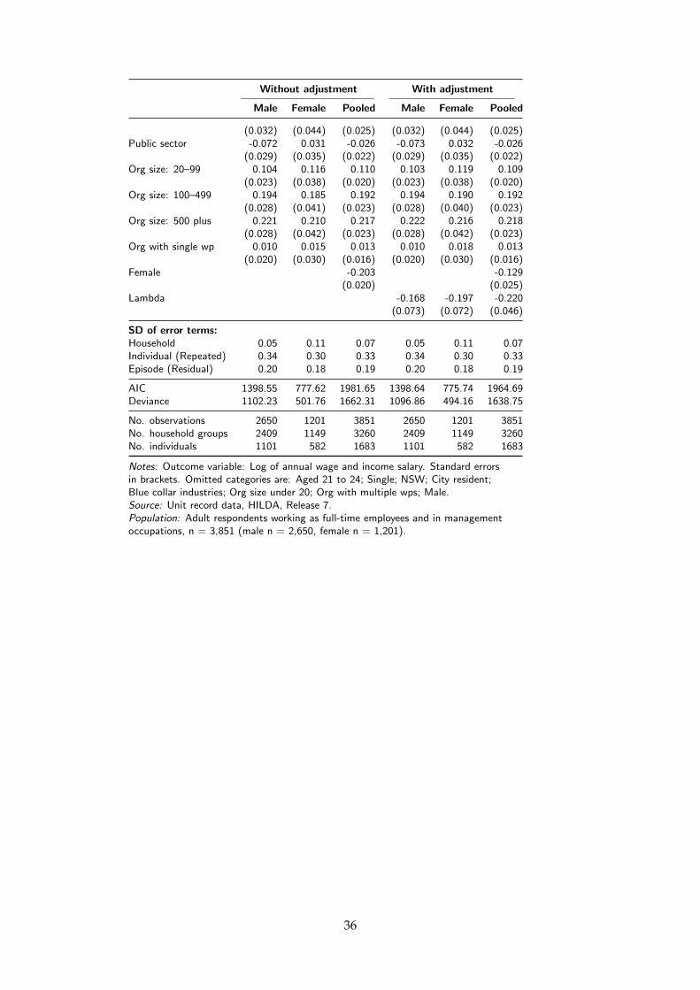