the hellinger–kantorovich distance and ......and define the hellinger–kantorovich distance hk...
TRANSCRIPT

Copyright © by SIAM. Unauthorized reproduction of this article is prohibited.
SIAM J. MATH. ANAL. c� 2016 Society for Industrial and Applied Mathematics
Vol. 48, No. 4, pp. 2869–2911
OPTIMAL TRANSPORT IN COMPETITION WITH REACTION:THE HELLINGER–KANTOROVICH DISTANCE
AND GEODESIC CURVES⇤
MATTHIAS LIERO† , ALEXANDER MIELKE‡ , AND GIUSEPPE SAVARE§
Abstract. We discuss a new notion of distance on the space of finite and nonnegative measureson ⌦ ⇢ Rd, which we call the Hellinger–Kantorovich distance. It can be seen as an inf-convolutionof the well-known Kantorovich–Wasserstein distance and the Hellinger-Kakutani distance. The newdistance is based on a dynamical formulation given by an Onsager operator that is the sum of aWasserstein di↵usion part and an additional reaction part describing the generation and absorptionof mass. We present a full characterization of the distance and some of its properties. In particular,the distance can be equivalently described by an optimal transport problem on the cone space overthe underlying space ⌦. We give a construction of geodesic curves and discuss examples and theirgeneral properties.
Key words. dissipation distance, geodesic curves, cone space, optimal transport, Onsageroperator, reaction-di↵usion equations
AMS subject classifications. 28A33, 46E27, 49K21, 49Q20, 58E30
DOI. 10.1137/15M1041420
1. Introduction. Starting from the pioneering works [11, 12], the reinterpreta-tion of certain scalar di↵usion equations as so-called Wasserstein gradient flows ledto new analytic tools and concepts and gave deeper insight into di↵usion problems;see, e.g., [1, 29]. In particular, in connection with suitable convexity properties ofthe driving functional the abstract theory of gradient flows in metric space developedin [2] provides a sound and comprehensive geometric framework for these evolutionequations.
The recent reformulation of classes of reaction-di↵usion systems as gradient sys-tems (see [15, 20, 21]) raises the question of whether the abstract metric theory canbe also developed for this wider class of problems. A similar question was attackedin [5] for a McKean–Vlasov equation without mass conservation.
Following [20] we understand a gradient system as a triple (X,F,K) consisting ofa state space X, a driving functional F, and an Onsager operator K. The latter meansthat K is a state-dependent, symmetric, and positive semidefinite linear operator. Inmany cases the Onsager operator K induces a dissipation distance DK on the statespace X by minimizing an action functional over all curves connecting two states.Now, the development of a metric theory rests upon the ability to characterize this
⇤Received by the editors September 25, 2015; accepted for publication (in revised form) June 17,2016; published electronically August 30, 2016.
http://www.siam.org/journals/sima/48-4/M104142.htmlFunding: The first author’s research was partially supported by the Einstein Foundation Berlin
via the ECMath/Matheon project SE2. The second author’s research was partially supported by theDFG via project C5 within CRC 1114 (Scaling cascades in complex systems) and by the ERC underAdG267802 AnaMultiScale. The third author’s research was partially supported by PRIN10/11grant from the MIUR for the project Calculus of Variations.
†Research Group Partial Di↵erential Equations, Weierstraß-Institut fur Angewandte Analysis undStochastik, 10117 Berlin, Germany ([email protected]).
‡Research Group Partial Di↵erential Equations, Weierstraß-Institut fur Angewandte Analysis undStochastik, 10117 Berlin, Germany, and Institut fur Mathematik, Humboldt-Universitat zu Berlin,12489 Berlin-Adlershof, Germany ([email protected]).
§Department of Mathematics, Universita di Pavia, 27100 Pavia, Italy ([email protected]).
2869
Dow
nloa
ded
03/0
7/17
to 1
32.2
39.1
.231
. Red
istri
butio
n su
bjec
t to
SIA
M li
cens
e or
cop
yrig
ht; s
ee h
ttp://
ww
w.si
am.o
rg/jo
urna
ls/o
jsa.
php
Copyright © by SIAM. Unauthorized reproduction of this article is prohibited.
2870 M. LIERO, A. MIELKE, AND G. SAVARE
distance and its properties.This paper together with the companion paper [17] provides a rigorous charac-
terization of such a dissipation distance. While a very general theoretical backgroundis developed in that paper, the focus of the present work lies in the motivation of thetheory and explicit examples highlighting the induced geometry, which is based onthe simple Onsager operator
K↵,�
(u)⇠ = �↵ div(ur⇠) + �u⇠,
where ↵,� � 0 are fixed parameters. Obviously, the Onsager operator K↵,�
=↵KWass+�Kc-a is a sum of a Wasserstein part for di↵usion and a creation-annihilationpart, which is the simplest case of a reaction term. For the latter part it is not di�-cult to develop a corresponding analogue to the Wasserstein distance W. For this, wesimply note that Kc-a is the inverse of a metric tensor such that the formal associatedRiemannian structure is given by v 7!
R
⌦v2/(�u) dx. Thus, it is easy to see that
the Riemannian distance induced by K0,� is a multiple of the Hellinger–Kakutanidistance H; see [10, 13] and [28], where also the correct function spaces are discussed.In particular, for measures of the form µ
j
= fj
dx we obtain
D0,�(µ0, µ1) =2p�H(µ0, µ1) with H(µ0, µ1)
2 =
Z
⌦
⇣
p
f0 �p
f1⌘2
dx.
Of course, this distance generalizes to the space of finite, nonnegative Borel measures,denoted by M(⌦); see section 2.3. In the following we shall always assume that thedomain ⌦ ⇢ Rd is convex and compact.
We will show that K↵,�
generates a proper distance D↵,�
on M(⌦), which isformally given in a generalized Benamou–Brenier formulation (see [3]), i.e., by mini-mizing over all su�ciently smooth curves s 7! µ(s) connecting measures µ0 and µ1,namely
D↵,�
(µ0, µ1)2 = inf
⇢
Z 1
0
Z
⌦
⇥
↵|r⇠|2 + �⇠2⇤
dµ(s) ds�
�
�
ddsµ+ ↵ div(µr⇠) = �µ⇠, µ0
µ µ1
�
.
This characterization also works for reaction-di↵usion systems; see [15, sect. 2(e)].We call D
↵,�
the Hellinger–Kantorovich distance, since it can be understood asan inf-convolution (weighted by ↵ and �) of the Kantorovich–Wasserstein distance Wand the Hellinger distance H. In particular, geodesic curves for the distance D
↵,�
willoptimize the usage of transport against the usage of creation or annihilation. As anoutcome of our theory we will find that transport never occurs over distances longerthan ⇡
p
↵/�.For the rest of this introduction we will use the special choice ↵ = 1 and � = 4,
which simplifies the notation considerably.To give a full characterization of D1,4, we go on a detour which will highlight the
underlying geometry of the distance much better. Motivated by an explicit formulafor the distance between two Dirac measures, we introduce the cone space C⌦ over⌦ and define the Hellinger–Kantorovich distance HK(µ0, µ1) by lifting the measuresµj
to measures �j
on the cone and then minimizing the Wasserstein distance WC
induced by a suitable cone distance on C⌦. It is then easy to show that HK is indeeda geodesic distance, since W
C
is a geodesic distance. It is the purpose of section 4 to
Dow
nloa
ded
03/0
7/17
to 1
32.2
39.1
.231
. Red
istri
butio
n su
bjec
t to
SIA
M li
cens
e or
cop
yrig
ht; s
ee h
ttp://
ww
w.si
am.o
rg/jo
urna
ls/o
jsa.
php

Copyright © by SIAM. Unauthorized reproduction of this article is prohibited.
HELLINGER–KANTOROVICH DISTANCE AND GEODESIC CURVES 2871
show that D1,4 indeed equals HK. A similar result is given in [17] for general metricspaces, which is based on a characterization via the Hamilton–Jacobi equation. Here,we provide a di↵erent proof suited for Rd, which uses the continuity equation; cf. thedefinition of D
↵,�
above.For this proof, we will rely on a third characterization of the Hellinger–Kantoro-
vich distance, which is given in terms of the entropy-transport functional for calibra-tion measures ⌘ 2 M(⌦⇥⌦) given via
E1,4(⌘;µ0, µ1) :=
Z
⌦
FB
✓
d⌘0dµ0
◆
dµ0 +
Z
⌦
FB
✓
d⌘1dµ1
◆
dµ1 +
Z
⌦⇥⌦
c1,4(|x0�x1|)d⌘,
where FB(z) = z log z � z + 1, ⌘i
= ⇧i
#⌘ denote the usual marginals, and the costfunction c1,4 is given by
c1,4(L) :=
⇢
�2 log�
cosL�
for L < ⇡/2,1 for L � ⇡/2.
Since E1,4(·;µ0, µ1) is convex, it is easy to find minimizers; see [17] for more detailsand the proof that HK(µ0, µ1)2 = min{E1,4(⌘;µ0, µ1) | ⌘ 2 M(⌦⇥ ⌦) }.
To be more specific, we return to the question of computing the distance betweentwo Dirac masses µ
j
= aj
�y
j
with yj
2 ⌦ and aj
� 0. Looking at connecting curves ofthe form µ(s) = a(s)�
x(s) we can indeed minimize the length of these one-mass-point(1mp) curves and find the result
(1.1) D1mp(a0�y0, a1�y1
)2 =
(
a0 + a1 � 2pa0a1 cos(|y1�y0|) for |y1�y0| ⇡,
a0 + a1 + 2pa0a1 for |y1�y0| � ⇡.
In fact, a minimizer exists only for |y1�y0| < ⇡, where for |y1�y0| � ⇡ the valueD1mp(a0�y0
, a1�y1) is an infimum only. However, it will turn out that these curves are
only optimal for |y1�y0| ⇡/2, while for |y1�y0| > ⇡/2, the two-mass point curveµ(s) = (1�s)2a0�y0
+ s2a1�y1is shorter, since its squared length is a0 + a1. Thus,
creation and annihilation are better than transport in this case.Moreover, the formula in (1.1) suggests introducing a cone distance d
C
on the coneC⌦ over ⌦ given by the elements [x, r] for r > 0 and the tip o which is an identificationof { [x, 0] | x 2 ⌦ }. The cone distance is defined as
dC
([x0, r0], [x1, r1])2 := r20 + r21 � 2r0r1cos⇡(|x1�x0|) with cos
b
a = cos�
min{|a|, b}�
;
see [4, sect. 3.6.2]. This distance is again a geodesic distance, and we can define theassociated Wasserstein distance W
C
; see section 3.2.2.Based on this observation we can now lift measures µ on ⌦ to measures � on C⌦
such that µ = P�, where the projection P : M2(C⌦) ! M(⌦) is defined viaZ
⌦
�(x)d(P�)(x) =
Z
C⌦
r2�(x)d�([x, r]) for all � 2 C0(⌦).
Now, the first definition of the Hellinger–Kantorovich distance is
(1.2) HK(µ0, µ1) = min
⇢
WC
(�0,�1)�
�
�
P�0 = µ0, P�1 = µ1
�
.
To further analyze this construction, one needs to study the optimality conditions forthe lifts, which can be done by exploiting the characterization via E1,4; see Theorem 7and section 3.3.3, where the crucial duality theory is taken from [17].
Dow
nloa
ded
03/0
7/17
to 1
32.2
39.1
.231
. Red
istri
butio
n su
bjec
t to
SIA
M li
cens
e or
cop
yrig
ht; s
ee h
ttp://
ww
w.si
am.o
rg/jo
urna
ls/o
jsa.
php

Copyright © by SIAM. Unauthorized reproduction of this article is prohibited.
2872 M. LIERO, A. MIELKE, AND G. SAVARE
In section 4 we finally show the identity D1,4 = HK by a full characterization of allabsolutely continuous curves with respect to the distance HK; see Theorem 17. Thisis done by lifting curves in M(⌦) to curves in M2(C⌦) and using a characterizationof absolutely continuous curves with respect to W
C
which can be found in [18]. InCorollary 16 we obtain the important result that all geodesic curves in (M(⌦),HK)are obtained as projections
µ(s) = P�(s), where � : [0, 1] ! M2(C⌦)
is a geodesic curve in (M2(C⌦),WC
) connecting optimal lifts �0 and �1 in (1.2).Throughout this work, the notion “geodesic curve,” or shortly “geodesic,” meansconstant-speed minimal geodesic, namely
HK(µ(s), µ(t)) = |s�t|HK(µ(0), µ(1)) for all s, t 2 [0, 1].
Section 5 is devoted to various examples for geodesic curves, which are obtainedby doing optimal lifts to the cone space C⌦ and then constructing geodesic curves forthe Wasserstein distance W
C
and projecting them down. Since the geodesic curveson the cone C⌦ are explicit, this provides an explicit formula for geodesic curvesµ : [0, 1] ! M(⌦), as soon as the lifts are specified.
In particular, using this explicit construction we show that the total mass m(s) =µ(s)(⌦) along geodesic curves is 2-convex and 2-concave, since we have the identity
(1.3) m(s) = (1�s)m(0) + sm(1)� s(1�s)HK(µ0, µ1)2.
We discuss geodesic ⇤-convexity of some functionals; in particular, we show that thelinear functional F(µ) =
R
⌦�(x) dµ(x) is geodesically ⇤-convex if and only if the
function [x, r] 7! r2�(x) is geodesically ⇤-convex in (C⌦, dC).It is also worth noting that the unique geodesic connecting µ1 to the null measure
µ0 ⌘ 0, which has the lifts ↵�o
for ↵ � 0, is done by the unique Hellinger geodesic
µH(s) = s2µ1.
This simple observation immediately shows that the logarithmic entropy given byF(µ) =
R
⌦FB(u(x)) dx for µ = u dx is not geodesically ⇤-convex, since the second
derivative of
]0, 1[ 3 s 7! F(s2µ) = s2F(µ) + s2 log(s2)µ(⌦) + 1�s2
is not bounded from below. The general question of geodesic ⇤-convexity will bestudied in [16]; see also Remark 21.
In section 5.2 we reconsider our standard example of the geodesic connections ofDirac masses µ
j
= aj
�y
j
. It turns out that in the critical case |y0�y1| = ⇡/2 thereis an infinite-dimensional convex set of geodesic curves that can be constructed byshowing that there are many optimal lifts to the cone space C⌦.
Section 5.3 provides a generalization of the classical dilation of measures in theWasserstein case. For the Hellinger–Kantorovich distance there is a similar dilationwhere the mass inside the ball {x | |x�y0| < ⇡/2 } is radially transported and partlyannihilated into the point y0 while the mass at larger distance is simply annihilatedaccording to the Hellinger distance.
In section 5.4 we show how the transport of two characteristic functions occurs inthe Hellinger–Kantorovich case. While the too distant parts are simply annihilated
Dow
nloa
ded
03/0
7/17
to 1
32.2
39.1
.231
. Red
istri
butio
n su
bjec
t to
SIA
M li
cens
e or
cop
yrig
ht; s
ee h
ttp://
ww
w.si
am.o
rg/jo
urna
ls/o
jsa.
php

Copyright © by SIAM. Unauthorized reproduction of this article is prohibited.
HELLINGER–KANTOROVICH DISTANCE AND GEODESIC CURVES 2873
or created according to the Hellinger metric, the parts that are close enough lead toa continuous transition; see Figure 8.
In section 5.5 we show that the Hellinger–Kantorovich geodesic between two mea-sures µ0 and µ1 is unique if one of the two measures is absolutely continuous withrespect to the Lebesgue measure. Finally, section 5.6 shows that HK is not semicon-cave in M(⌦) if ⌦ ⇢ Rd has dimension two or higher, which is in sharp contrast tothe Wasserstein distance; see [2, Def. 12.3.1].
This work, together with its companion paper [17], will form the basis of subse-quent work where we will explore the metric properties of the the space (M(⌦),HK)and study gradient systems on this space. In particular, in the spirit of [15], we aimto establish a metric theory for scalar reaction-di↵usion equations of the form
u = �K↵,�
(u)�F(u) = div�
↵ur(�F(u)�
� �u�F(u),
where �F denotes a variational derivative; see the work [16] in preparation.Note during final preparation. The earliest parts of the work presented here were
first presented at the ERC Workshop on Optimal Transportation and Applicationsin Pisa in 2012. Since then, the authors developed the theory continuously furtherand presented results at di↵erent workshops and seminars. We refer the reader to [17,sect. A] for some remarks concerning the chronological development. In June, 2015,they became aware of the parallel work [14]. Moreover, in mid-August, 2015, theybecame aware of [6, 7]. So far, these independent works are not reflected in the presentversion of this paper.
2. Gradient structures for reaction-di↵usion equations.
2.1. General philosophy for gradient systems. We call a triple (X,F, )a gradient system in the di↵erentiable sense if X is a Banach space containing thestates u, if the functional F : X ! R1 := R [ {1} has a Frechet subdi↵erentialDF(u) 2 X⇤ on a suitable subset of X, and if is a dissipation potential. The lastmeans that (u, ·) : X ! [0,1] is a lower semicontinuous and convex functional with (u, 0) = 0. Denoting by ⇤(u, ·) : X⇤ ! [0,1] the Legendre–Fenchel transform ⇤(u, ⇠) = sup{ h⇠, vi � (u, v) | v 2 X }, the gradient evolution is given via
(2.1) u 2 D⇠
⇤(u,�DF(u)) or equivalently 0 = Du
(u, u) + DF(u).
For simplicity, we assume that the Frechet subdi↵erential DF and the convex sub-di↵erentials D
u
and D⇠
⇤ are single-valued, but the set-valued case can be treatedsimilarly by the standard generalizations.
If the map v 7! (u, v) is quadratic, we call the above system a classical gradientsystem, while otherwise we speak of generalized gradient systems. In the classicalcase we can write
(u, v) =1
2hG(u)v, vi and ⇤(u, ⇠) =
1
2h⇠,K(u)⇠i,
where G(u) : X ! X⇤ and K(u) : X⇤ ! X are symmetric and positive (semi-)definite operators. Since and ⇤ form a dual pair, we have G(u)�1 = K(u) andK(u)�1 = G(u) if we interpret these identities in the sense of quadratic forms. Wecall G the Riemannian operator, as it generalizes the Riemannian tensor on finite-dimensional manifolds, while we call K the Onsager operator, because of Onsager’sfundamental contributions in justifying gradient systems via his reciprocal relations
Dow
nloa
ded
03/0
7/17
to 1
32.2
39.1
.231
. Red
istri
butio
n su
bjec
t to
SIA
M li
cens
e or
cop
yrig
ht; s
ee h
ttp://
ww
w.si
am.o
rg/jo
urna
ls/o
jsa.
php

Copyright © by SIAM. Unauthorized reproduction of this article is prohibited.
2874 M. LIERO, A. MIELKE, AND G. SAVARE
K(u) = K(u)⇤; cf. [22, eqs. (1.11)–(1.12)] or [23, eqs. (2-1)–(2-4)]. Thus, for classicalgradient systems the general form (2.1) specializes to
(2.2) u = �K(u)DF(u) or equivalently G(u)u = �DF(u).
We emphasize that K(u) maps (a subspace of) X⇤ to X, so generalized thermo-dynamic driving forces are mapped to rates. Similarly, G(u) maps rates to viscousdissipative forces, which have to balance the potential restoring force �DF(u).
Our work follows the same philosophy as in [12, 25]: Even though the abovegradient structure is only formal, it may generate a new dissipation distance, whichcan be made rigorous such that finally the gradient structure can be considered as amathematically sound metric gradient flow, as discussed in [2]. For this, one intro-duces the dissipation distance associated with the dissipation potential , which isdefined via
DK(u0, u1)2 := inf
⇢
Z 1
0
hG(u)u, uids�
� u 2 H1([0, 1];X), u(j) = uj
�
.
2.2. Dissipation distances for reaction-di↵usion systems. It was shownin [20] that certain reaction-di↵usion systems admit a formal gradient structure, whichis given by an Onsager operator K and a driving functional F of the form
K(c)⇠ = � div(M(c)r⇠) +H(c)⇠, F(c) =
Z
⌦
I
X
i=1
F (ci
)dx,
where c = (ci
)i=1,...,I is the vector of nonnegative concentrations of the species X
i
,i = 1, . . . , I, and M(c) and H(c) are a symmetric and positive definite mobility tensorand a reaction matrix, respectively. With the di↵usion tensor D(c) = M(c)D2F(c)and the reaction term R(c) = H(c)DF(c) the generated gradient-flow equation readsas
c = �K(c)DF(c) = div�
D(c)rc�
�R(c).
As in the theory of the Kantorovich–Wasserstein distance (cf. [12, 24, 25, 29]) theoperator K(c) can be seen as the inverse of a metric tensor G(c) that gives rise to a
geodesic distance between two densities c0, c1 2 L1(⌦; [0,1[I) defined abstractly via
(2.3) DK(c0, c1)2 := inf
⇢
Z 1
0
hK(c(t))�1c(t), c(t)idt�
�
�
c0c c1
�
.
Here, “c0c c1” means that t 7! c(t) is a su�ciently smooth curve with c(0) = c0
and c(1) = c1.Since in general the inversion of K is di�cult or even not well-defined, it is better
to use the following formulation in terms of the dual variable ⇠(s) = K(c(s))�1c(s),namely
(2.4) DK(c0, c1)2 := inf
⇢
Z 1
0
h⇠(t),K(c(t))⇠(t)idt�
�
�
c = K(c)⇠, c0c c1
�
.
In our case of reaction-di↵usion operators we can make this even more explicit, namely
(2.5)
DK(c0, c1)2 := inf
⇢
Z 1
0
Z
⌦
r⇠ : M(c)r⇠ + ⇠ ·H(c)⇠dxdt�
�
�
c = � div(M(c)r⇠�
+H(c)⇠, c0c c1
�
.
Dow
nloa
ded
03/0
7/17
to 1
32.2
39.1
.231
. Red
istri
butio
n su
bjec
t to
SIA
M li
cens
e or
cop
yrig
ht; s
ee h
ttp://
ww
w.si
am.o
rg/jo
urna
ls/o
jsa.
php

Copyright © by SIAM. Unauthorized reproduction of this article is prohibited.
HELLINGER–KANTOROVICH DISTANCE AND GEODESIC CURVES 2875
Finally, we can use the Benamou–Brenier argument [3] to find the following charac-terization (cf. [15, sect. 2.5]).
Proposition 1. We have the equivalence(2.6)
DK(c0, c1)2 = inf
⇢
Z 1
0
Z
⌦
⌅ : M(c)⌅+ ⇠ ·H(c)⇠dx dt�
�
�
c = � div�
M(c)⌅�
+H(c)⇠, c0c c1
�
= inf
⇢
Z 1
0
Z
⌦
P : M(c)�1P + s ·H(c)�1s dx dt�
�
�
c = � div(P ) + s, c0c c1
�
,
where ⇠(t, x) = H(c(t, x))�1s(t, x) 2 RI and ⌅(t, x) = M(c(t, x))�1P (t, x) 2 RI⇥d.
Proof. Clearly, the right-hand side in (2.6) gives a value that is smaller than orequal to that in (2.5), because we have dropped the constraint ⌅ = r⇠.
To show that the two definitions give the same value, we have to show that forminimizers (if they exist), the constraint ⌅ = r⇠ is automatically satisfied. For thiswe use that ⇠ and ⌅ are related by the continuity equation c = � div(M(c)⌅
�
+H(c)⇠.Keeping c fixed (and su�ciently smooth) we can minimize the integral in (2.6)
with respect to ⇠ and ⌅, which is a quadratic functional with an a�ne constraint.Hence, we can apply the Lagrange multiplier rule to
L(⌅, ⇠,�) =
Z 1
0
Z
⌦
⌅ : M(c)⌅+ ⇠ ·H(c)⇠ + � ·�
c+ div(M(c)⌅�
�H(c)⇠�
dxdt
to obtain the Euler–Lagrange equations
0 = 2 eM⌅�Mr�, 0 = 2H⇠ �H�, 0 = c+ div(M(c)⌅�
�H(c).
From the first two equations we conclude that ⌅ = 12r� = r⇠, which is the desired
result.
2.3. Scalar reaction-di↵usion equations. On ⌦ ⇢ Rd, which is a boundedand convex domain, we consider scalar equations of the form
u = div(a(u)ru)� f(u) in ⌦, ru · ⌫ = 0 on @⌦,
where we assume that f changes sign, such that f(u)(u�1) is positive for u 2 ]0, 1[ []1,1[. We want to write the above equation as a gradient system (X,F,K) withX = L1(⌦),
F(u) =
Z
⌦
F (u(x))dx, and K(u)⇠ = � div�
µ(u)r⇠�
+ k(u)⇠ with r⇠ · ⌫ = 0,
where F : R ! [0,1] is a strictly convex function with F (u) = 1 for u < 0 andF (1) = 0. Moreover, we assume µ(u), k(u) � 0 such that the dual dissipation poten-tial is the nonnegative quadratic form
⇤(u, ⇠) =
Z
⌦
µ(u(x))
2|r⇠(x)|2 + k(u(x))
2⇠(x)2dx.
Dow
nloa
ded
03/0
7/17
to 1
32.2
39.1
.231
. Red
istri
butio
n su
bjec
t to
SIA
M li
cens
e or
cop
yrig
ht; s
ee h
ttp://
ww
w.si
am.o
rg/jo
urna
ls/o
jsa.
php

Copyright © by SIAM. Unauthorized reproduction of this article is prohibited.
2876 M. LIERO, A. MIELKE, AND G. SAVARE
Using DF(u) = F 0(u(x)) we obtain
K(u)DF(u) = � div�
µ(u)F 00(u)ru�
+ k(u)F 0(u).
Hence we see that we obtain the above reaction-di↵usion equation if we choose F, µ,and k such that the relations
a(u) = µ(u)F 00(u) and k(u)F 0(u) = f(u).
There are several canonical choices. Quite often one is interested in the casea ⌘ 1, which gives rise to the simple semilinear equation u = �u � f(u). To realizethis, one chooses µ(u) = 1/F 00(u). This is particularly interesting in the case of thelogarithmic entropy where F (u) = FB(u) := u log u�u+1. Then µ(u) = 1/F 00(u) = uand we obtain the Wasserstein operator ⇠ 7! � div(ur⇠) for the di↵usion part.
For the reaction part, one simply chooses k(u) = f(u)/F 0(u), which is positive,since f(u) and F 0(u) change the sign at u = 1. For F = FB and the equation
u = �u� (u� � u↵) with 0 ↵ < �
we obtain k(u) = (u� � u↵)/ log u = (��↵)⇤(u↵, u�), where the logarithmic meanis given via ⇤(a, b) = (a�b)/(log a� log b). This equation models the evolution of asingle di↵using species undergoing the creation-annihilation reaction
↵X*)
�X.
The simplest example of a reaction-di↵usion distance is the Hellinger–Kantorovichdistance D
↵,�
studied in section 3 in great detail. It is defined via the scalar Onsageroperator
(2.7) K↵,�
(c)⇠ := �↵ div(cr⇠) + � c ⇠,
where ↵,� are nonnegative parameters. The special property of this operator isthat it is linear in the variable c. This will allow us to do explicit calculations forthe corresponding dissipation distance D
↵,�
:= DK↵,�
. In particular, the associateddistance is defined for all pairs of (nonnegative and finite) measures µ0, µ1 2 M(⌦),not just for probability measures P(⌦). In fact, we will see that for � > 0 the geodesiccurves connecting two di↵erent probability measures will have mass less than one forall arclength parameters s 2 ]0, 1[.
For � = 0 we obtain the scaled Kantorovich–Wasserstein distance, namely
D↵,0(µ0, µ1) =
8
>
<
>
:
1p
↵|µ0|W⇣ µ0
|µ0|,µ1
|µ1|
⌘
if |µ0| = |µ1|,
1 else.
Here, |µj
| = µj
(⌦) is the total mass of the measure. The geodesic curves are given interms of the classical optimal transport; see [2, Chap. 7].
For ↵ = 0 we obtain a scaled version of the Hellinger distance (sometimes alsocalled Hellinger–Kakutani distance), namely
D0,�(µ0, µ1) =2p�H(µ0, µ1) =
2p�
Z
⌦
⇣dµ0
dµ⇤
⌘1/2
�⇣dµ1
dµ⇤
⌘1/2�2
dµ⇤
!1/2Dow
nloa
ded
03/0
7/17
to 1
32.2
39.1
.231
. Red
istri
butio
n su
bjec
t to
SIA
M li
cens
e or
cop
yrig
ht; s
ee h
ttp://
ww
w.si
am.o
rg/jo
urna
ls/o
jsa.
php

Copyright © by SIAM. Unauthorized reproduction of this article is prohibited.
HELLINGER–KANTOROVICH DISTANCE AND GEODESIC CURVES 2877
for a reference measure µ⇤ with µi
⌧ µ⇤ (e.g., µ⇤ = µ0 + µ1); see [28, Thm. 4]. Thegeodesic curves are given by linear interpolation of the square roots of the densities,i.e.,
(2.8)�
µH(s)�
(A) =
Z
A
(1�s)
✓
dµ0
d(µ0+µ1)
◆1/2
+ s
✓
dµ1
d(µ0+µ1)
◆1/2!2
d(µ0+µ1).
By using the estimate µH(s) � (1�s)2µ0 + s2µ1 and choosing s 2 [0, 1] optimally,we obtain the lower estimate |µH(s)| � |µ0||µ1|/(|µ0|+|µ1|); i.e., the total mass ofthe geodesic µH(s) is bounded from below by half of the harmonic mean of the totalmasses of µ0 and µ1. Moreover, an elementary calculation gives the identity
(2.9) |µH(s)| = (1�s)|µ0|+ s|µ1|� s(1�s)H(µ0, µ1)2.
3. The Hellinger–Kantorovich distance. In this section we discuss the dis-sipation distance D
↵,�
(µ0, µ1) that is induced by the Onsager operator K↵,�
(c)⇠ =� div(↵cr⇠) + �c⇠, given for µ0, µ1 2 M(⌦) as in (2.3). Using Proposition 1 we canrewrite this formulation in an equivalent form as
(3.1)
D↵,�
(µ0, µ1)2 = inf
⇢
Z 1
0
Z
⌦
⇥
↵|⌅|2 + �⇠2⇤
dµ(s) ds�
�
�
d
dsµ+ ↵ div(µ⌅) = �µ⇠, µ0
µ µ1
�
with ⌅ : [0, 1]⇥ ⌦! Rd denoting the vector field.In most of this section we will restrict ourselves without loss of generality to
the case ↵ = 1 and � = 4 for simplicity. Occasionally, we will give some of theformulas for general ↵ and � to highlight the dependence on these parameters. Notethat we can always use the simple scaling K
↵,�
= �K↵/�,1 giving the general relation
D↵,�
(µ0, µ1) = D↵/�,1(µ0, µ1)/
p�. Moreover, the factor
p
↵/� can be transformed
away by rescaling ⌦, i.e., x 7!p
↵/�x.Note that for su�ciently regular µ, ⇠, and ⌅ in (3.1) we obtain by Proposition 1
⌅ = r⇠ and formal calculation leads to the following system of equations for geodesiccurves:
µ = �↵ div(µr⇠) + �µ⇠, ⇠ +↵
2|r⇠|2 + �
2⇠2 = 0.(3.2)
For the case � = 0 and ↵ = 1 this corresponds to [3, eq. (37)]. A full justification ofthis coupled system is given in [17, sect. 8.6].
3.1. The optimal curves for D↵,� with one or two mass points. Thestriking feature of optimal transport is that for a�ne mobilities point masses (Diracmeasures) are transported as point masses, i.e., the geodesic curve connecting µ0 = �
x0
and µ1 = �x1
is given by µs
= �x(s), where [0, 1] 3 s 7! x(s) is a geodesic curve in the
underlying domain ⌦.Since the Onsager operator K
↵,�
(c) in (2.7) depends only linearly on the state c,we expect a similar behavior. In particular, note that the definition of the distancein (3.1) is well-defined for general curves of measures µ(s) 2 M(⌦) if we understandthe linear constraint d
dsµ+ ↵ div(µ⌅) = �µ⇠ in the distributional sense.
Dow
nloa
ded
03/0
7/17
to 1
32.2
39.1
.231
. Red
istri
butio
n su
bjec
t to
SIA
M li
cens
e or
cop
yrig
ht; s
ee h
ttp://
ww
w.si
am.o
rg/jo
urna
ls/o
jsa.
php

Copyright © by SIAM. Unauthorized reproduction of this article is prohibited.
2878 M. LIERO, A. MIELKE, AND G. SAVARE
As a first step, it is instructive to study the K↵,�
-length of curves given by amoving point mass in the form
�x,a
: [0, 1] 3 s 7! µ(s) = a(s)�x(s) with x(s) 2 ⌦ and a(s) � 0.
Minimizing the action functional in (3.1) only over curves of this form for given endpoints a
i
�x
i
, i = 0, 1, always gives an upper bound for the distance D↵,�
(a0�x0, a1�x1
).Indeed, we show that up to a certain threshold for the Euclidean distance |x0�x1| itwill even be the exact distance and the minimizing �
x,a
is a geodesic curve.The main point is that we are able to calculate the s-derivative of µ(s) = �
x,a
(s)and compare it to the continuity equation. Multiplying the continuity equation withtest functions we obtain after integration by parts
d
dsµi
(s) = � div�
x(s)a(s)�x(s)
�
+ a(s)�x(s) = � div
�
x(s)µ(s)�
+a(s)
a(s)µ(s).
Thus, comparing with the continuity equation in the definition of D↵,�
we find therelations
(3.3) ⌅(s, x(s)) =1
↵x(s) and ⇠(s, x(s)) =
a(s)
�a(s).
We may realize the constraint ⌅ = r⇠ via ⇠(s, y) = ⇠(s, x(s)) + 1↵
x(s) · (y�x(s)).Having identified the vector and scalar field ⌅ and ⇠, respectively, we obtain the
K↵,�
-length of the curve s 7! a(s)�x(s) via
(3.4) Length↵,�
(�x,a
)2 =
Z 1
0
1
↵|x(s)|2 + 1
�
✓
a(s)
a(s)
◆2�
a(s)ds;
for ↵ = 0 and � = 8 this corresponds to the representation in [28, Thm. 4] for theHellinger–Kakutani distance. Minimizing this expression for given end points of �
x,a
we find that x(s) travels along a straight line, which reflects the fact that our choiceof metric in ⌦ is the Euclidean one. However, the speed will not be constant. Hence,we introduce functions
⇢ 2 R(0, 1) := { ⇢ 2 H1(0, 1) | ⇢(0) = 0, ⇢(1) = 1, ⇢ � 0 },a 2 A(a0, a1) := { a 2 H1(0, 1) | a > 0, a(0) = a0, a(1) = a1 }
(3.5)
such that we can write x(s) = (1�⇢(s))x0 + ⇢(s)x1 and have |x(s)| = ⇢(s)L with L =|x1�x0|. For the 1mp problem we define the function J1mp
↵,�
: [0,1[⇥ [0,1[2 ! [0,1[via
(3.6) J1mp↵,�
(L2, a0, a1) := inf
⇢
Z 1
0
L2
↵⇢(s)2a(s) +
a(s)2
�a(s)ds
�
�
�
⇢ 2 R(0, 1), a 2 A(a0, a1)
�
.
The functional J1mp↵,�
satisfies a scaling identity with respect to the parameter ↵,� > 0:For ✓ > 0 we have
(3.7) J1mp↵,�
(L2, a0, a1) =1
✓J1mp1,�/✓
✓
✓L2
↵, a0, a1
◆
.
Dow
nloa
ded
03/0
7/17
to 1
32.2
39.1
.231
. Red
istri
butio
n su
bjec
t to
SIA
M li
cens
e or
cop
yrig
ht; s
ee h
ttp://
ww
w.si
am.o
rg/jo
urna
ls/o
jsa.
php

Copyright © by SIAM. Unauthorized reproduction of this article is prohibited.
HELLINGER–KANTOROVICH DISTANCE AND GEODESIC CURVES 2879
Fig. 1. The function s 7! ⇢(s) in Theorem 2 for di↵erent ratios a
0
/a
1
and L = ⇡/1.1 ( right)and L = ⇡/2 ( left). The dashed curve corresponds to a
0
/a
1
= 1, while curves above and belowsatisfy a
0
/a
1
< 1 and a
0
/a
1
> 1, respectively.
Hence, we can restrict ourselves to one particular choice of �/✓ > 0 such that thegeneral case can be recovered from a rescaling of the Euclidean distance in ⌦. Inparticular, it will prove convenient to choose ✓ = �/4 such that we will consider J1mp
1,4
first, which is also the scaling used in [17].
Theorem 2. We have
(3.8)
J1mp1,4 (L2, a0, a1) = a0 + a1 � 2
pa0a1 cos⇡(L) with
cos⇡
(L) :=
⇢
cos(L) for L < ⇡,�1 for L � ⇡.
The infimum is a minimum for L < ⇡, and it is attained for
a(s) = (1�s)2a0 + s2a1 + 2s(1�s)pa0a1 cos(L),
⇢(s) =
8
>
>
<
>
>
:
1L
arctan�
s sin(L)pa1
(1�s)pa0+s cos(L)
pa1
�
if (1�s)pa0+s cos(L)
pa1 > 0,
⇡
2L if (1�s)pa0+s cos(L)
pa1 = 0,
1L
arctan�
s sin(L)pa1
(1�s)pa0+s cos(L)
pa1
�
+ ⇡
L
otherwise.
(3.9)
For L � ⇡ the minimizing sequences converge to a(s) = c(s�✓)2 and ⇢(s) = �✓
(s) forcertain c � 0 and ✓ 2 [0, 1]; see Figures 1 and 2 for an illustration of a and ⇢.
Proof. To study the infimum of J1mp1,4 we transform the system by using b(s) =
p
a(s). Keeping L > 0 fixed we obtain the functional
KL
(b, ⇢) =
Z 1
0
L2 b(s)2 ⇢(s)2 + b(s)2ds.
Clearly, the infimum of KL
gives the infimum in the definition of J1mp1,4 . We now
consider a minimizing sequence (bn
, ⇢n
) and observe that (bn
) must remain boundedin H1(0, 1). Hence, after choosing a suitable subsequence (not relabeled), we mayassume b
n
* b in H1(0, 1). We distinguish between the following three cases.
Case 1: b := min{ b(s) | s 2 [0, 1] } > 0. In this case we may further concludethat ⇢
n
is also bounded in H1(0, 1). Hence, we can also assume ⇢n
* ⇢ in H1(0, 1).Because of the lower semicontinuity of K
L
on H1(0, 1)2 we conclude that (b, ⇢) is the
Dow
nloa
ded
03/0
7/17
to 1
32.2
39.1
.231
. Red
istri
butio
n su
bjec
t to
SIA
M li
cens
e or
cop
yrig
ht; s
ee h
ttp://
ww
w.si
am.o
rg/jo
urna
ls/o
jsa.
php

Copyright © by SIAM. Unauthorized reproduction of this article is prohibited.
2880 M. LIERO, A. MIELKE, AND G. SAVARE
Fig. 2. Top: The curves s 7! (LRs
0
⇢(⌧)d⌧, a(s)) for di↵erent values of 0 < L < ⇡. Solid curvesare true geodesics, while dashed curves are shortest “1mp paths” but not geodesic curves. Bottom:The curves for L = ⇡/2 and di↵erent mass ratios a
0
/a
1
.
global minimizer of KL
. This implies that (a, ⇢) = (b2, ⇢) is the global minimizer ofJ1mp1,4 , which certainly satisfies the Euler–Lagrange equations
dds
�
⇢a�
= 0, 4�
L⇢�2 �
�
a/a�2 � 2 d
ds
�
a/a�
= 0.
From the first equation andR 1
0⇢ds = 1 we obtain
⇢(s) = H[a]/a(s), where H[a] =
✓
Z 1
0
1/a(s)ds
◆�1
denotes the harmonic mean, which satisfies H[a] � b2 > 0. By inserting this into thesecond equation we see that all solutions are given in the form
a(s) = c0 + c1(s�✓)2 with c0c1 = L2H[a]2.
Hence, together with the boundary conditions a0 = a(0) = c0 + c1✓2 and a1 = a(1) =c0+c1(1�✓)2 we have three nonlinear equations for the unknowns c0, c1, and ✓, whichcan be solved easily for L < ⇡ giving a unique solution. For L � ⇡ no solution withpositive b exists. In particular, since the primitive of the inverse of a strictly positivequadratic function is given in terms of the arctan function, we obtain the formulas in(3.9), using also the addition theorem for arctan.
Thus, in the case b > 0 the global minimizer is the unique, positive critical point(a, ⇢).
Case 2: b = 0. Since b is continuous, there exists s⇤ 2 [0, 1] with b(s⇤) = 0.Neglecting the term L2b2⇢2 in the integrand in K
L
we can minimize the remainingquadratic term subject to the boundary conditions b(0) =
pa0, b(1) =
pa1, and
b(s⇤) = 0. This leads to a minimizer that is piecewise a�ne and gives the lower
Dow
nloa
ded
03/0
7/17
to 1
32.2
39.1
.231
. Red
istri
butio
n su
bjec
t to
SIA
M li
cens
e or
cop
yrig
ht; s
ee h
ttp://
ww
w.si
am.o
rg/jo
urna
ls/o
jsa.
php

Copyright © by SIAM. Unauthorized reproduction of this article is prohibited.
HELLINGER–KANTOROVICH DISTANCE AND GEODESIC CURVES 2881
bound
(3.10) KL
(b, ⇢) � a0s⇤
+a1
1�s⇤��p
a0 +pa1�2,
where the last estimate follows from minimization in s⇤.It is now easy to see that the value
�pa0 +
pa1�2
is indeed the infimum, since itcan be obtained as a limit of a minimizing sequence. For this, take piecewise a�nefunctions (b
n
, ⇢n
) satisfying (bn
(s), ⇢n
(s)) = (0, n) for s 2 [sn
, sn
+1/n] with sn
! s0,where s0 is the optimal s⇤ in (3.10). On [0, s
n
] we take (bn
(s), ⇢(s)) = (�pa0/sn, 0)
and similarly on [sn
+1/n, 1].
General case: Since the infimum obtained in Case 2 is strictly larger than thatin Case 1 (because of L < ⇡), we see that the two cases exclude each other. IfL < ⇡, then Case 1 occurs, while for L � ⇡, Case 2 sets in. Hence, the theorem isestablished.
Although the stationary states in Theorem 2 may be the global minimizers, theyare not always the geodesic curves with respect to D1,4. To see this we consider thepure reaction case and define the curve
b�a0,a1
(s) = a0(s)�x0+ a1(s)�x1
also connecting the measures µj
= aj
�x
j
if aj
(j) = aj
and aj
(1�j) = 0 for j = 0, 1. Ifa0(s), a1(s) > 0, this curve consists of two separated mass points that do not move.As in the previous case of the moving mass point we can compute the solutions of thecontinuity equation to obtain
⌅ ⌘ 0 and ⇠(s, xj
) =aj
(s)
4aj
(s).
The squared length of these curves is given by 14
P
j
R 1
0a2j
/aj
ds, and the optimal
choice for aj
is a0(s) = a0(1�s)2 and a1(s) = a1s2 giving the minimal squared length
Length1,4(b�opt)2 = a0 + a1 � D1,4(a0�x0 , a1�x1).
We see that this result is less than J1mp1,4 (|x1�x0|2, a0, a0) for ⇡/2 < |x1�x0| < ⇡. In
fact, we will show later that the last estimate is sharp if and only if |x1�x0| � ⇡/2.To highlight the dependencies on ↵ and � in J1mp
↵,�
we can use the scaling (3.7)for all ↵,� > 0. To include the limit cases of the Hellinger distance (i.e., ↵ = 0) andthe Kantorovich–Wasserstein distance (i.e., � = 0) we define the functions S
↵,�
via(3.11)
S
↵,�
(L2, b0, b1) :=
8
>
>
>
>
>
>
>
>
<
>
>
>
>
>
>
>
>
:
4�
⇣
b20 + b21 � 2b0b1cos⇡�
q
�
4↵ L�
⌘
if ↵, � > 0,4�
�
b20 + b21�
if ↵=L=0 and � > 0,
L
2
↵
b20 if �=0, ↵>0 and b1=b0,
0 if ↵=�=L=0 and b0=b1,
1 otherwise.
We emphasize that S0,� and S
↵,0 can be obtained as �-limits of S↵
n
,�
n
for �n
& 0or ↵
n
& 0, respectively.Using S
↵,�
we can express J1mp↵,�
for all ↵, � � 0, where the cases ↵ = 0 or
� = 0 mean that ⇢ ⌘ 0 or a ⌘ 0, respectively. Moreover, J1mp↵,�
= +1 if the set ofcompetitors (a, ⇢) providing finite values is empty.
Dow
nloa
ded
03/0
7/17
to 1
32.2
39.1
.231
. Red
istri
butio
n su
bjec
t to
SIA
M li
cens
e or
cop
yrig
ht; s
ee h
ttp://
ww
w.si
am.o
rg/jo
urna
ls/o
jsa.
php
Copyright © by SIAM. Unauthorized reproduction of this article is prohibited.
2882 M. LIERO, A. MIELKE, AND G. SAVARE
Corollary 3. For all ↵, � � 0 we have
J1mp↵,�
(L2, a0, a1) = S
↵,�
�
L2,pa0,
pa1�
.
Proof. We only need to consider the boundary cases. For ↵ = � = 0 we havea ⌘ 0 ⌘ ⇢, which implies that J1mp
0,0 is finite only for L = 0 and a0 = a1.For ↵ = 0 and � > 0 we have ⇢ ⌘ 0 and obtain a finite value only for L = 0.
Clearly, the infimum ofR 1
0a2/(�a) ds is given by 4(
p
a(1)�p
a(0))2/�, which is thedesired result.
The case � = 0 and ↵ > 0 provides a ⌘ 0 and ⇢ ⌘ 1. Hence, the infimum isL2a0/↵ for a1 = a0 and 1 otherwise.
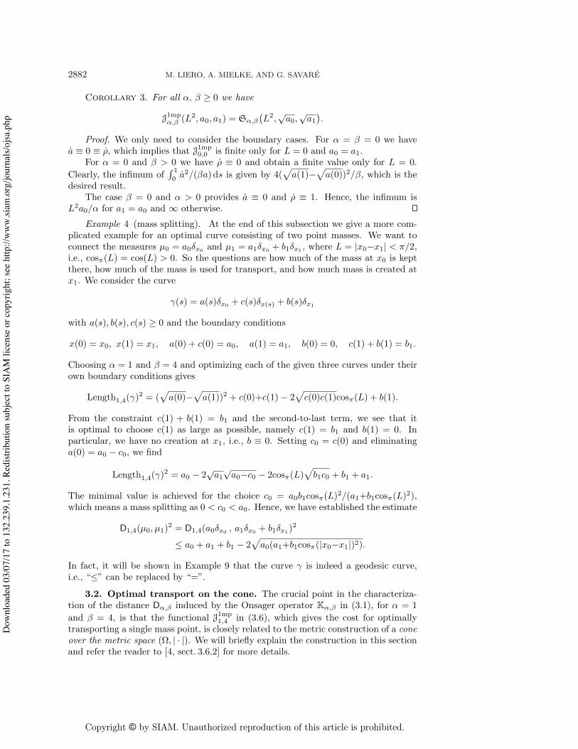
Example 4 (mass splitting). At the end of this subsection we give a more com-plicated example for an optimal curve consisting of two point masses. We want toconnect the measures µ0 = a0�x0
and µ1 = a1�x0+ b1�x1
, where L = |x0�x1| < ⇡/2,i.e., cos
⇡
(L) = cos(L) > 0. So the questions are how much of the mass at x0 is keptthere, how much of the mass is used for transport, and how much mass is created atx1. We consider the curve
�(s) = a(s)�x0
+ c(s)�x(s) + b(s)�
x1
with a(s), b(s), c(s) � 0 and the boundary conditions
x(0) = x0, x(1) = x1, a(0) + c(0) = a0, a(1) = a1, b(0) = 0, c(1) + b(1) = b1.
Choosing ↵ = 1 and � = 4 and optimizing each of the given three curves under theirown boundary conditions gives
Length1,4(�)2 = (
p
a(0)�p
a(1))2 + c(0)+c(1)� 2p
c(0)c(1)cos⇡
(L) + b(1).
From the constraint c(1) + b(1) = b1 and the second-to-last term, we see that itis optimal to choose c(1) as large as possible, namely c(1) = b1 and b(1) = 0. Inparticular, we have no creation at x1, i.e., b ⌘ 0. Setting c0 = c(0) and eliminatinga(0) = a0 � c0, we find
Length1,4(�)2 = a0 � 2
pa1pa0�c0 � 2cos
⇡
(L)p
b1c0 + b1 + a1.
The minimal value is achieved for the choice c0 = a0b1cos⇡(L)2/(a1+b1cos⇡(L)2),which means a mass splitting as 0 < c0 < a0. Hence, we have established the estimate
D1,4(µ0, µ1)2 = D1,4(a0�x0
, a1�x0+ b1�x1
)2
a0 + a1 + b1 � 2p
a0(a1+b1cos⇡(|x0�x1|)2).
In fact, it will be shown in Example 9 that the curve � is indeed a geodesic curve,i.e., “” can be replaced by “=”.
3.2. Optimal transport on the cone. The crucial point in the characteriza-tion of the distance D
↵,�
induced by the Onsager operator K↵,�
in (3.1), for ↵ = 1and � = 4, is that the functional J1mp
1,4 in (3.6), which gives the cost for optimallytransporting a single mass point, is closely related to the metric construction of a coneover the metric space (⌦, | · |). We will briefly explain the construction in this sectionand refer the reader to [4, sect. 3.6.2] for more details.
Dow
nloa
ded
03/0
7/17
to 1
32.2
39.1
.231
. Red
istri
butio
n su
bjec
t to
SIA
M li
cens
e or
cop
yrig
ht; s
ee h
ttp://
ww
w.si
am.o
rg/jo
urna
ls/o
jsa.
php

Copyright © by SIAM. Unauthorized reproduction of this article is prohibited.
HELLINGER–KANTOROVICH DISTANCE AND GEODESIC CURVES 2883
0 y1
y2
x
r
Fig. 3. The cone C
[0,3⇡/2]
represented as sector in R2 via (y1
, y
2
) = (r cosx, r sinx) and threegeodesic curves. The angle x = ⇡ is critical for smoothness of geodesic curves.
Given the closed and convex domain ⌦ ⇢ Rd, we construct the cone C⌦ as thequotient of ⌦⇥ [0,1[ over ⌦⇥ {0}, i.e.,
C⌦ :=�
⌦⇥ [0,1[�
.
�
⌦⇥ {0}�
.
In particular, all points in ⌦⇥{0} are identified with one point, namely the tip of thecone denoted by o. For any x 2 ⌦ and r > 0, the equivalence classes are denoted byz = [x, r] 2 C⌦, while for r = 0 the equivalence class [x, 0] is equal to o.
Motivated by the previous section we define the distance dC
: C⌦ ⇥ C⌦ ! [0,1[on the cone space C⌦ as follows:
dC
([x0, r0], [x1, r1])2 := r20 + r21 � 2r0r1cos⇡(|x1�x0|),
where cos⇡
is defined as in Theorem 2.For the special case that ⌦ = [0, `] ⇢ R with 0 < ` < 2⇡, we can visualize
C⌦ = C[0,`] by the two-dimensional sector
⌃`
:= { y = (r cosx, r sinx) 2 R2 | r � 0, x 2 [0, `] },
where y = (0, 0) corresponds to the tip o. The induced distance is the Euclidiandistance restricted to ⌃
`
; i.e., the geodesic curve between y0 and y1 is a straightsegment if |x1�x0| ⇡, while it consists of the two rays connecting y = 0 with y0 andy1, respectively, if ⇡ |x1�x0| ` < 2⇡; see Figure 3. In the case of the travelingmass point discussed in the previous section we identify the Dirac measures a
i
�x
i
withpairs [x
i
,pai
] 2 C⌦. Thus, the result of Theorem 2 can be reformulated as
J1mp1,4 (|x0�x1|2; a0, a1) = d
C
�
[x0,pa0], [x1,
pa1]
�2.
For general coe�cients ↵,� > 0, the distance dC
has to be replaced by
d↵,�C
(z0, z1) = d↵,�C
([x0, r0], [x1, r1]) =q
S
↵,�
(|x1�x0|, r0, r1);
see (3.11). This distance can be seen as a geodesic distance on the cone C⌦ inducedby a Riemannian metric (outside of the vertex o) given by the tensor
(3.12) GC
↵,�
([x, r]) :=
✓
r
2
↵
IRd 00 4/�
◆
2 R(d+1)⇥(d+1).
This fact is already seen in (3.4) if we set a(s) = r(s)2.
Dow
nloa
ded
03/0
7/17
to 1
32.2
39.1
.231
. Red
istri
butio
n su
bjec
t to
SIA
M li
cens
e or
cop
yrig
ht; s
ee h
ttp://
ww
w.si
am.o
rg/jo
urna
ls/o
jsa.
php

Copyright © by SIAM. Unauthorized reproduction of this article is prohibited.
2884 M. LIERO, A. MIELKE, AND G. SAVARE
3.2.1. Geodesic curves in the cone space. As shown in [4, sect. 3.6.2], thepair (C⌦, dC) is a complete geodesic space, where each two points can be connectedby a unique arclength-parameterized geodesic curve. These curves are given by thefollowing geodesic interpolator Z(s; ·, ·) : C⌦ ⇥ C⌦ ! C⌦ (recall z
j
= [xj
, rj
]):
Z(s; z0, z1) := [X(s; z0, z1), R(s; z0, z1)], where
R(s; z0, z1)2 := (1�s)2r20 + s2r21 + 2s(1�s)r0r1cos⇡(|x0�x1|),
X(s; z0, z1) :=�
1�⇢(s; z0, z1)�
x0 + ⇢(s; z0, z1)x1,
(3.13)
and ⇢ : [0, 1]⇥ C⌦ ⇥ C⌦ ! [0, 1] is defined via
⇢(s; z0, z1) :=
8
>
<
>
:
1
|x1�x0|arccos
⇣ (1�s)r0 + sr1 cos |x1�x0|R(s; z0, z1)
⌘
for |x1�x0| < ⇡,
1
2
⇣
1 + sign�
(1�s)r0 � sr1�
⌘
for |x1�x0| � ⇡.
Note that in the definition of R there is a “+” in front of the cosine term, while thereis a “�” in the distance d
C
. Moreover, by elementary geometric identities it is easyto see that the formula for ⇢ is equivalent to that obtained in Theorem 2.
In particular, the curve defined by �(s) = Z(s; z0, z1) is a constant speed geodesiccurve with respect to the distance d
C
connecting z0 and z1, i.e.,
(3.14) 8 0 s < t 1: dC
�
�(s), �(t)�
= |t�s|dC
(z0, z1).
As for the Wasserstein–Kantorovich distance, the geodesic curves in C⌦ are key forthe construction of the geodesic curves with respect to the Hellinger–Kantorovichdistance. We will discuss this in section 3.4 in detail.
3.2.2. The transport distance modulo reservoirs on the cone space.Using the theory of optimal transport (cf. [2, 29]) we can define the Kantorovich–Wasserstein distance W
C
associated with the cone distance dC
on the set of all non-negative and finite measures M2(C⌦) as follows. If �0(C⌦) 6= �1(C⌦), then we setW
C
(�0,�1) = 1, and otherwise we set
WC
(�0,�1)2 := inf
⇢
ZZ
C⌦⇥C⌦
dC
(z0, z1)2 d�(z0, z1)
�
�
�
� 2 M(C⌦⇥C⌦), ⇧i
#� = �i
�
.
Moreover, there the geodesic interpolation (which is not unique in general) can bedescribed using an optimal transport plan � that is a minimizer in the definition ofW
C
. We denote the geodesic interpolator by
(3.15) Z�
(s;�0,�1) := Z(s; ·, ·)#�.
For the proper handling of creation and annihilation of mass we introduce amodified distance. The modification occurs via a reservoir of mass in the vertex o ofthe cone such that mass is generated from the reservoir and absorbed into it. Thefollowing result shows that if we assume that the reservoir is su�ciently big (and inour model for the Hellinger–Kantorovich operator it is in fact infinite), we never haveany true transport over distances larger than ⇡/2 (respectively,
p
↵/�⇡ in the scaledcase), which is only half the critical distance of possible transport; see Figure 4.
Proposition 5 (optimal transport in the presence of large reservoirs). Weconsider arbitrary measures �0,�1 2 M2(C⌦) with equal masses �0(C⌦) = �1(C⌦):
Dow
nloa
ded
03/0
7/17
to 1
32.2
39.1
.231
. Red
istri
butio
n su
bjec
t to
SIA
M li
cens
e or
cop
yrig
ht; s
ee h
ttp://
ww
w.si
am.o
rg/jo
urna
ls/o
jsa.
php

Copyright © by SIAM. Unauthorized reproduction of this article is prohibited.
HELLINGER–KANTOROVICH DISTANCE AND GEODESIC CURVES 2885
(a) The function [0,1[ 3 7! w(�0,�1,) := WC
(�o
+�0,�o+�1) is nonin-creasing.
(b) Define the real numbers
✓j
:= �j
(C⌦\o), ⇢j
:= �j
({o}), and ⇤ = max{0, ✓1�⇢0, ✓0�⇢1};
then for all � ⇤ we have w(�0,�1,) = w(�0,�1,⇤) with similar transportplans di↵ering only by (�⇤)�o,o.
(c) For any optimal transport plan � connecting ⇤�o+�0 and ⇤�o+�1 we have�(N) = 0, where
N :=�
(z0, z1) 2 C⌦⇥C⌦
�
� r0, r1 > 0, |x0�x1| > ⇡/2
;
i.e., there is no transport in ⌦ over distances longer than ⇡/2.
Proof. Part (a). Let 0 1 < 2 be given, and let �1 , �2 2 M2(C⌦⇥C⌦) be
optimal transport plans for the pairs 1�o+�i and 2�o+�i, i = 0, 1, respectively.Since 2 > 1, we can define the transport plan b�
2= (2�1)�(o,o) + �
1, which
satisfies ⇧i
#b�2= 2�o + �
i
. Thus, b�2
is an admissible plan for the minimizationproblem in the definition of W
C
and we obtain the estimate
w(�0,�1,2)2 = W
C
(2�o+�0,2�o+�1)2
ZZ
C⌦⇥C⌦
dC
(z0, z1)2db�
2(z0, z1)
=
ZZ
C⌦⇥C⌦
dC
(z0, z1)2d�
1(z0, z1) = w(�0,�1,1)2.
Hence, 7! w(�0,�1,) is not increasing.Part (b). Let �
and �⇤ denote the optimal transport plans with respect to
and ⇤, respectively. Similar to (a) we define the measure b�⇤ = �
� (�⇤)�(o,o).Obviously, b�
⇤ satisfies ⇧i
#b�⇤ = �i
+⇤�o. It remains to show that b�⇤ is nonnegative
and hence is an admissible transport plan. Indeed, due to the estimate �
({o}⇥(C⌦ \{o})) ✓1 and the definition of ⇤ we obtain
�
({o}⇥{o}) = �
({o}⇥C⌦)� �
�
{o}⇥(C⌦ \ {o})�
� + ⇢0 � ✓1 � � ⇤.
Hence, b�⇤ � 0 and, arguing as for (a), we get w(�0,�1,⇤) w(�0,�1,). However,
due to the first part of the theorem even equality must hold.Part (c). As before let � denote an optimal plan for lifts ⇤�o+�0 and ⇤�o+�1
of µ0 and µ1. Assume that �(N) > 0 such that dC
(z0, z1)2 > r20 + r21 for �-a.a.(z0, z1) 2 N with z
i
= [xi
, ri
]. We aim to construct a new transport plan b� based on� giving a strictly lower cost and hence showing the nonoptimality of �.
To this end, we introduce the characteristic function � of the subset N
c :=(C⌦⇥C⌦) \ N. Moreover, we denote by e�
i
2 M2(C⌦) the marginals of e��
= ��,which are obviously absolutely continuous with respect to �
i
. We denote the den-sities with ⇢
i
such that e�i
= ⇢i
�i
. In particular, for �i
-a.e. z 2 C⌦ we have that0 ⇢
i
1.We define the measure b�:
b�(dz0, dz1) = e��
(dz0, dz1) + (1�⇢0)�0(dz0)�o(dz1) + �o
(dz0)(1�⇢1)�1(dz1).
We easily check that the marginals of b� are given by b�i
= �i
+ �o
, i = 0, 1, where > 0 is given by = (��e�
�
)(C⌦⇥C⌦). In particular, b�i
is an admissible lift for µi
.
Dow
nloa
ded
03/0
7/17
to 1
32.2
39.1
.231
. Red
istri
butio
n su
bjec
t to
SIA
M li
cens
e or
cop
yrig
ht; s
ee h
ttp://
ww
w.si
am.o
rg/jo
urna
ls/o
jsa.
php

Copyright © by SIAM. Unauthorized reproduction of this article is prohibited.
2886 M. LIERO, A. MIELKE, AND G. SAVARE
It remains to show that b� has a strictly lower cost than �. We computeZZ
C⌦⇥C⌦
dC
(z0, z1)2db� =
ZZ
C⌦⇥C⌦
dC
(z0, z1)2de�
�
+
Z
C⌦
r20(1�⇢0)d�0 +Z
C⌦
r21(1�⇢1)d�1
=
ZZ
N
c
dC
(z0, z1)2d� +
ZZ
N
�
r20 + r21�
d�
<
ZZ
C⌦⇥C⌦
dC
(z0, z1)2d�.
Thus, � cannot be optimal and any optimal transport plan has to vanish on N.
Using the above proposition we may define a new distance Wrsv on M2(C⌦) thatassumes that the reservoir is always big enough. Indeed, we define
Wrsv(�0,�1) := inf>0
WC
(�0+�o,�1+�o) = WC
(�0+⇤�o,�1+⇤�o),
where ⇤ is given as in Proposition 5(b).
3.3. The Hellinger–Kantorovich distance. We can now easily define a dis-tance for measures on ⌦ by lifting measures µ
j
2 M(⌦) to measures on M2(C⌦)and projecting back measures from M2(C⌦) into M(⌦). We define the projectionP : M2(C⌦) ! M(⌦) via
Z
⌦
�(x)dP� =
Z
C⌦
r2�(x)d�([x, r]) for all � 2 C0(⌦).
In the last formula we use that for r > 0 the equivalence class [x, r] uniquely determinesx and r and that the prefactor r2 makes the function � : [x, r] 7! r2�(x) continuousif we set �(o) = 0. In the case µ = P� we call � a lift of µ.
The first and most intuitive result on the distance D1,4 induced by the Onsageroperator K1,4 in (3.1) is the following formula, which we formulate as a definition firstand then show that it equals the distance D1,4.
Definition 6. The Hellinger–Kantorovich distance on M(⌦) is defined as
(3.16) HK(µ0, µ1) = min
⇢
WC
(�0,�1)�
�
�
P�0 = µ0, P�1 = µ1
�
.
Before proving the identity HK = HK1,4 = D1,4 in section 4, we collect someproperties of HK. First, we emphasize that the projection P does not see the reservoirsat o, and hence the above formula already includes arbitrary reservoirs according toProposition 5.
Next, let us remark that HK satisfies an important scaling invariance: Let # : C⌦⇥C⌦ ! ]0,1[ be a Borel map, and define the dilation function h
#
: C⌦⇥C⌦ ! C⌦⇥C⌦
via
(3.17) h#
(z0, z1) =
✓
x0,r0
#(z0, z1)
�
,
x1,r1
#(z0, z1)
�◆
for zi
= [xi
, ri
].
Then, given any transport plan � 2 M2(C⌦⇥C⌦), we define the dilated plan �#
=(h
#
)#(#2 �) in M(C⌦⇥C⌦). Letting �i
and �#i
denote the marginals of � and �#
wehave that
(3.18)
ZZ
C⌦⇥C⌦
dC
(z0, z1)2d� =
ZZ
C⌦⇥C⌦
dC
(z0, z1)2d�
#
and P�i
= P�#i
.
Dow
nloa
ded
03/0
7/17
to 1
32.2
39.1
.231
. Red
istri
butio
n su
bjec
t to
SIA
M li
cens
e or
cop
yrig
ht; s
ee h
ttp://
ww
w.si
am.o
rg/jo
urna
ls/o
jsa.
php
Copyright © by SIAM. Unauthorized reproduction of this article is prohibited.
HELLINGER–KANTOROVICH DISTANCE AND GEODESIC CURVES 2887
In particular, we can always assume that the transport plans � and the lifts �i
areprobability measures, e.g., by setting # ⌘ (�(C⌦⇥C⌦))�1/2.
The main result of this section is the following structural theorem. For a full proofwe refer the reader to [17], where a more general case is considered. In particular,there ⌦ is replaced by general complete geodesic spaces. However, because of thestrong relevance of part (v) for the subsequent applications, we present a di↵erentproof of the identity HK = D1,4 in section 4 which is adapted to the case Rd.
Theorem 7 (properties of HK). The distance HK : M(⌦) ⇥M(⌦) ! [0,1[ hasthe following properties:
(i) For each pair µ0, µ1 there exists an optimal pair �0,�1 of lifts.(ii) For all measures µ0, µ1 the upper bound HK(µ0, µ1)2 µ0(⌦) + µ1(⌦) is
satisfied.(iii) (M(⌦),HK) is a complete and separable metric space.(iv) The topology induced by HK coincides with the weak topology on M(⌦).(v) The distance HK is induced by the Onsager operator K1,4.
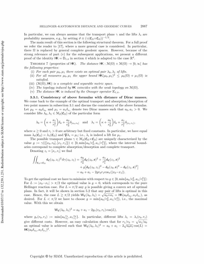
3.3.1. Consistency of above formulas with distance of Dirac masses.We come back to the example of the optimal transport and absorption/desorption oftwo point masses in subsection 3.1 and discuss the consistency of the above formulas.Let µ0 = a0�x0 and µ1 = a1�x1 denote two Dirac masses such that a0, a1 > 0. Weconsider lifts �0,�1 2 M2(C⌦) of the particular form
�0 =
✓
+a1r21
◆
�o
+a0r20�[x0,r0] and �1 =
✓
+a0r20
◆
�o
+a1r21�[x1,r1],
where � 0 and ri
> 0 are arbitrary but fixed constants. In particular, we have equalmass �0(C⌦) = �1(C⌦) and P�
i
= µi
; i.e., �i
is indeed a lift for µi
.The possible transport plans � 2 M2(C⌦⇥C⌦) are uniquely characterized by the
value g := �({[x0, r0], [x1, r1]}) 2 [0,min{a0/r20, a1/r21}], where the interval bound-aries correspond to complete absorption/desorption and complete transport.
Denoting zi
= [xi
, ri
] we findZZ
C⌦⇥C⌦
dC
(z0, z1)2d�(z0, z1) =
a0r20
dC
(z0, o)2 +
a1r21
dC
(z1, o)2
+ g⇥
dC
(z0, z1)2 � d
C
(z0, o)2 � d
C
(z1, o)2⇤
= a0 + a1 � 2gr0r1cos⇡(|x0�x1|).
To get the optimal cost we have to minimize with respect to g 2 [0,min{a0/r20, a1/r21}]:For L := |x0�x1| > ⇡/2 the optimal value is g = 0, which corresponds to the pureHellinger reaction case. For L = ⇡/2 any g is possible giving a convex set of optimalplans. In fact, it will be shown in section 5.2 that any pair of lifts is optimal in thiscase. Hence, the case L � ⇡/2 yields W
C
(�0,�1) =pa0+a1 = HK(a0�x0
, a1�x1), as
desired. For L < ⇡/2 we have to choose g = min{a0/r20, a1/r21}, i.e., the maximalvalue. With this we obtain
WC
(�0,�1)2 = a0 + a1 � 2g⇤(r0, r1) cos(L),
where g⇤(r0, r1) := min{a0 r1
r0, a1
r0
r1}. In particular, di↵erent lifts �
i
= �i
(r0, r1)
give di↵erent costs. However, an easy calculation shows that for r1/r0 =p
a1/a0an optimal value is achieved such that W
C
(�0,�1)2 = a0 + a1 � 2pa0a1 cos(L) =
HK(a0�x0, a1�x1
)2.
Dow
nloa
ded
03/0
7/17
to 1
32.2
39.1
.231
. Red
istri
butio
n su
bjec
t to
SIA
M li
cens
e or
cop
yrig
ht; s
ee h
ttp://
ww
w.si
am.o
rg/jo
urna
ls/o
jsa.
php
Copyright © by SIAM. Unauthorized reproduction of this article is prohibited.
2888 M. LIERO, A. MIELKE, AND G. SAVARE
For calculating the distance HK the particular choice of an optimal lift is notimportant, but we will see in section 5.2 that in the case L = ⇡/2 di↵erent liftsmay give rise to di↵erent geodesic curves. Hence, we highlight here that even in thetrivial case L < ⇡/2 there are many optimal lifts. For example, for a1 = a0 > 0 any⌘ 2 M2([0,1[) with
R10
r2d⌘ = a0 defines optimal lifts �j
= �x
j
⌦⌘.
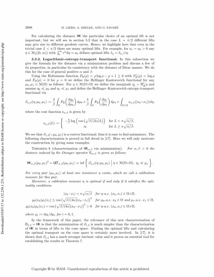
3.3.2. Logarithmic-entropy-transport functional. In this subsection wegive the formula for the distance via a minimization problem and discuss a few ofits properties, in particular its consistency with the distance of Dirac masses. We dothis for the case of general positive ↵ and �.
Using the Boltzmann function FB(⇢) = ⇢ log ⇢ � ⇢ + 1 � 0 with F 0B(⇢) = log ⇢
and FB(⇢) = 0 for ⇢ = 0 we define the Hellinger–Kantorovich functional for anyµ0, µ1 2 M(⌦) as follows. For ⌘ 2 M(⌦⇥⌦) we define the marginals ⌘
j
= ⇧j
#⌘ andassume ⌘0 ⌧ µ0 and ⌘1 ⌧ µ1 and define the Hellinger–Kantorovich entropy-transportfunctional via
E↵,�
(⌘;µ0, µ1) :=4
�
Z
⌦
FB
✓
d⌘0dµ0
◆
dµ0+4
�
Z
⌦
FB
✓
d⌘1dµ1
◆
dµ1+
Z
⌦⇥⌦
c↵,�
(|x0�x1|)d⌘,
where the cost function c↵,�
is given by
c↵,�
(L) :=
(
� 8�
log⇣
cos�
p
�/(4↵)L�
⌘
for L < ⇡p
↵/�,
1 for L � ⇡p
↵/�.
We see that E1,4(·;µ0, µ1) is a convex functional; thus it is easy to find minimizers. Thefollowing characterization is proved in full detail in [17]. Here we will only motivatethe construction by giving some examples.
Theorem 8 (characterization of HK↵,�
via minimization). For ↵,� > 0 thedistance induced by the Onsager operator K
↵,�
is given as follows:
HK↵,�
(µ0, µ1)2 = LET
↵,�
(µ0, µ1) := inf
⇢
E↵,�
(⌘;µ0, µ1)�
�
�
⌘ 2 M(⌦⇥⌦), ⌘j
⌧ µj
�
.
For every pair (µ0, µ1) at least one minimizer ⌘ exists, which we call a calibrationmeasure for this pair.
Moreover, a calibration measure ⌘ is optimal if and only if it satisfies the opti-mality conditions
|x0�x1| < ⇡p
↵/� for ⌘-a.e. (x0, x1) 2 ⌦⇥⌦,
%0(x0)%1(x1) cos�
p
�/(4↵)|x0�x1|�2
for µ0-a.e. x0 2 ⌦ and µ1-a.e. x1 2 ⌦,
%0(x0)%1(x1) = cos�
p
�/(4↵)|x0�x1|�2
> 0 for ⌘-a.e. (x0, x1) 2 ⌦⇥⌦,
where %i
:= d⌘i
/dµi
for i = 0, 1.
In the framework of this paper, the relevance of this new characterization ofD1,4 = HK is that the minimization of E1,4 is much simpler than the characterizationof HK in terms of lifts to the cone space. Finding the optimal lifts and calculatingthe optimal transport on the cone space is certainly more involved. In [17], it isshown that E1,4 has a much stronger intrinsic value and it proves an essential tool forestablishing the results in Theorem 7.
Dow
nloa
ded
03/0
7/17
to 1
32.2
39.1
.231
. Red
istri
butio
n su
bjec
t to
SIA
M li
cens
e or
cop
yrig
ht; s
ee h
ttp://
ww
w.si
am.o
rg/jo
urna
ls/o
jsa.
php

Copyright © by SIAM. Unauthorized reproduction of this article is prohibited.
HELLINGER–KANTOROVICH DISTANCE AND GEODESIC CURVES 2889
Example 9 (mass splitting, part 2). We return to Example 4, where we calculatedthe distance between
µ0 = a0�x0and µ1 = a1�x0
+ b1�x1
with L = |x0�x1| < ⇡ and ↵ = 1, � = 4. We show that the formulation in Theorem 8indeed gives the same cost. Since the marginals ⌘
j
have to have a density with respectto µ
j
and since ⌘0 and ⌘1 must have equal mass, we consider
⌘0 = e0�x0and ⌘1 = (e0�e1)�x0
+ e1�x1
with e0, e1 � 0. Using the formula in Theorem 8 yields for LET = LET1,4 and c = c1,4
LET(µ0, µ1) = inf{FB(e0
a0)a0 + FB(
e0�e1
a1)a1 + FB(
e1
b1)b1 + e1c(L) | e0 � e1 � 0 }.
This infimum can be evaluated explicitly, and we obtain
LET(µ0, µ1) = HK(µ0, µ1)2 = a0 + a1 + b1 � 2
p
a0(a1+b1 cos(|x0�x1|)2),
which is the same as in Example 4.
3.3.3. Reduction to special lifts. The characterization of the Hellinger–Kantorovich distance in terms of the logarithmic-entropy-transport functional givesrise to another helpful property: To calculate HK(µ0, µ1) it is su�cient to considerlifts �
i
of a special form only. Indeed, assume that ⌘ 2 M(⌦⇥⌦) is a minimizerof E1,4 for given µ0 and µ1 and consider for ⌘
i
= ⇧i
#⌘ the Lebesgue decomposition
µi
= �i
⌘i
+ µ?i
. Then the transport plan �⌘
2 M(C⌦⇥C⌦) defined by
�⌘
(dz0, dz1) = �p�0(x0)
(dr0)�p�1(x1)
(dr1)⌘(dx0, dx1)
+ �1(dr0)µ?0 (dx0)�o(dz1) + �
o
(dz0)�1(dr1)µ?1 (dx1)
and the associated lifts �i
= ⇧i
#�⌘ are optimal in Definition 6 for HK; see [17,Thm. 7.21] for the proof. In particular, we can restrict the analysis to lifts of µ
j
characterized by a single positive function brj
> 0 on ⌦, namely
L(µ, br,) = �o
+1
br(x)2�br(x)(dr)µ(dx) such that
Z
C⌦
�(z)dL(µ, br,) = �(o) +
Z
⌦
�([x, br(x)])
br(x)2dµ for all � 2 C0(C⌦).
We collect this observation in the following result.
Proposition 10 (HK via special lifts). We have the equivalent characterization
(3.19) HK(µ0, µ1) = min
⇢
WC
�
L(µ0, br0,0),L(µ1, br1,1)�
�
�
�
j
� 0, brj
> 0
�
.
Moreover, it is su�cient to consider transport plans � 2 M2(C⌦⇥C⌦) of the form
� = �br0(x0)(dr0)⌘0(dx0)�o(dz1) + �o
(dz0)�br1(x1)(dr1)⌘1(dx1)
+ �br0(x0)(dr0)�br1(x1)(dr1)⌘(dx0, dx1)
for positive functions bri
: ⌦! ]0,1[ and measures ⌘i
2 M(⌦) and ⌘ 2 M(⌦⇥ ⌦).
Dow
nloa
ded
03/0
7/17
to 1
32.2
39.1
.231
. Red
istri
butio
n su
bjec
t to
SIA
M li
cens
e or
cop
yrig
ht; s
ee h
ttp://
ww
w.si
am.o
rg/jo
urna
ls/o
jsa.
php

Copyright © by SIAM. Unauthorized reproduction of this article is prohibited.
2890 M. LIERO, A. MIELKE, AND G. SAVARE
Using the definition of WC
in terms of dC
and the form of the lifts, the functionalin (3.19) can be written as
D(⌘, br0, br1;µ0, µ1) := µ0(⌦) + µ1(⌦)�Z
⌦⇥⌦
2br0(x0)br1(x1) cos⇡/2 |x0�x1|d⌘(x0, x1),
and the following characterization of HK follows:
(3.20) HK(µ0, µ1)2 = min
⇢
D(⌘, br0, br1;µ0, µ1)�
�
�
⌘ 2 M(⌦⇥⌦),⇧j
#⌘ = br2j
µj
+ µ?j
�
.
We emphasize that not all optimal transport plans are of the form depicted inProposition 10. In particular, using again the example of two mass points we show insection 5.2 that in the case of the critical distance |x0�x1| lifts are quite arbitrary.
3.3.4. Recovering the Hellinger and Wasserstein–Kantorovich distance.The log-entropy formulation of the Hellinger–Kantorovich distance is well suited topass to the limits ↵! 0 or � ! 0.
Since apart from the prefactor 1/� the functional only depends on �/↵, we can set↵ = 1 and consider the case � ! 0. For the cost functional we obtain the expansion
c1,�(x0, x1) = |x1�x0|2 +O(�)
uniformly on ⌦⇥⌦, which is compact. Hence the linear transport functional convergesto the Kantorovich functional for the usual Euclidian cost function. Simultaneously,the entropic terms blow up, which means that in the limit � = 0 we obtain thecondition ⌘
j
= µj
. Thus, we expect to obtain the Wasserstein distance in the limit,i.e., HK1,0(µ0, µ1) = W(µ0, µ1).
Keeping � = 4 fixed and considering ↵! 0 we obtain
c↵,4(x0, x1) !
⇢
0 for x0 = x1,1 for x0 6= x1.
Thus, optimal calibration measures for ↵ = 0 will have support on the diagonal{ (x, x) 2 ⌦⇥⌦ | x 2 ⌦ } such that the transport cost equals 0 and that ⌫ := ⌘0 = ⌘1.Minimizing the sum of the two entropic terms with respect to ⌫, we obtain the uniquesolution ⌫ from the optimality condition d⌫
dµ0
d⌫dµ1
⌘ 1 and we find HK0,4(µ0, µ1) =
H(µ0, µ1) = kpµ1�pµ0kL2 .
3.4. Geodesic curves induced by optimal transport plans. Let µ0, µ1 2M(⌦) be two given measures. The geodesic curves with respect to the Hellinger–Kantorovich distance HK are induced by the geodesic curves in the underlying conespace.
More precisely, the construction of the geodesic curve s 7! µ(s) is based on thegeodesic interpolator Z defined in (3.13): Let �0 2 M2(C⌦) and �1 2 M2(C⌦) beoptimal lifts for µ0 and µ1, respectively, and let � 2 M2(C⌦⇥C⌦) be the associatedoptimal transport plan. Then a geodesic curve µ(s) = G(s;µ0, µ1) is obtained via theprojection of the geodesic curve for �0 and �1 in M2(C⌦) via
(3.21) µ(s) = G(s;µ0, µ1) := P�(s) with �(s) = Z(s; ·, ·)#�.
Note that since the optimal transport plan � is not necessarily unique, the geodesicsin M(⌦) are also not necessarily unique.
Dow
nloa
ded
03/0
7/17
to 1
32.2
39.1
.231
. Red
istri
butio
n su
bjec
t to
SIA
M li
cens
e or
cop
yrig
ht; s
ee h
ttp://
ww
w.si
am.o
rg/jo
urna
ls/o
jsa.
php

Copyright © by SIAM. Unauthorized reproduction of this article is prohibited.
HELLINGER–KANTOROVICH DISTANCE AND GEODESIC CURVES 2891
0 y1
y2
Fig. 4. Cone geodesic (dotted) for z
0
= [x0
,
pa
0
] and z
1
= [x1
,
pa
1
] compared to Hellinger–Kantorovich geodesic (solid) for µ
0
= a
0
�
x0 and µ
1
= a
1
�
x1 in the case |x0
�x
1
| > ⇡/2. TheHellinger–Kantorovich geodesic consists of two parts: one part is going to the reservoir (absorption),while the other one is simultaneously coming from the reservoir (generation).
Example 11. There are two ways that nonuniqueness of geodesics can occur. In(i) we give a case where the nonuniqueness is due to the nonuniqueness of the optimalcalibration measure ⌘ in Theorem 8 or in (3.20). This case is already present in theKantorovich–Wasserstein distance; see, e.g., [29, Rem. 9.5]. In (ii) we give a newsource of nonuniqueness, where ⌘ is unique, but the di↵erent lifts to the cone givedi↵erent geodesics. We refer the reader to section 5.5 for more details.
(i) On ⌦ = ]�2, 2[2 we choose the measures µ0 = �(�1,0) + �(1,0) and µ1 =�(0,�1) + �(0,1). For all ✓ 2 [0, 1] the curves
µ✓(s) = ✓a(s)⇥
�(1,0)+⇢(s)(�1,1) + �(�1,0)�⇢(s)(�1,1)
⇤
+ (1�✓)a(s)⇥
�(1,0)�⇢(s)(1,1) + �(�1,0)+⇢(s)(1,1)
⇤
are geodesics if a and ⇢ are as in Theorem 2.Moreover, if we choose µ1 to be the line measure concentrated in {0} ⇥]�1, 1[, the high symmetry of the optimization problem provides an infinite-dimensional convex set of optimal transport plans and hence of geodesiccurves; see [29, Rem. 9.5] for the analogue in the Kantorovich–Wassersteincase.
(ii) Consider the case of two mass points µi
= ai
�x
i
with |x0�x1| = ⇡/2. The onlyoptimal calibration measure is ⌘ = 0, and the distance equals HK(µ0, µ1) =�
a0+a1�1/2
. Moreover, one geodesic is the 1mp transport µ(s) = a(s)�x(s)
with x(s) = (1�⇢(s))x0+⇢(s)x1 and a(s) and ⇢(s) as in Theorem 2, while an-other geodesic connection is the pure Hellinger curve µH(s) = (1�s)2a0�x0
+s2a1�x1
. In section 5.2 we show that the set of all geodesic connections isinfinite dimensional.
Theorem 12. The curve s 7! µ(s) defined in (3.21) is a constant-speed geodesicwith respect to the Hellinger–Kantorovich distance HK, i.e.,
HK(µ(s), µ(t)) = |t�s|HK(µ0, µ1) for all 0 s < t 1.
Proof. Fix 0 s < t 1, and let � 2 M2(C⌦⇥C⌦) denote the optimal transportplan. We define the map ⇧
st
: C2⌦ ! C
2⌦ via ⇧
st
(z0, z1) = (Z(s; z0, z1), Z(t; z0, z1))and introduce the transport plan �
st
= (⇧st
)#� whose marginals are given by �(s)
Dow
nloa
ded
03/0
7/17
to 1
32.2
39.1
.231
. Red
istri
butio
n su
bjec
t to
SIA
M li
cens
e or
cop
yrig
ht; s
ee h
ttp://
ww
w.si
am.o
rg/jo
urna
ls/o
jsa.
php

Copyright © by SIAM. Unauthorized reproduction of this article is prohibited.
2892 M. LIERO, A. MIELKE, AND G. SAVARE
and �(t), respectively. In particular, we have the upper estimate
HK�
µ(s), µ(t)�
WC
�
�(s),�(t)�
✓
ZZ
C⌦⇥C⌦
dC
(z0, z1)2d�
st
◆1/2
.
However, using the definition of the �st
and that Z is the geodesic interpolator in C⌦
we obtain
(3.22) HK�
µ(s), µ(t)�
|s�t|HK(µ0, µ1) for all 0 s < t 1.
To see that equality actually holds we use the triangle inequality and (3.22) to find
HK(µ0, µ1) HK(µ0, µs
) + HK(µs
, µt
) + HK(µt
, µ1)
�
s+ (t�s) + (1�t)�
HK(µ0, µ1) = HK(µ0, µ1).
Thus, all inequalities are equalities, which proves the theorem.
4. Equivalence to the dynamical formulation. In this subsection we providethe proof of part (v) of Theorem 7 and show the equivalence of the two definitionsof the Hellinger–Kantorovich distance, namely the formulation via lifts and optimaltransport on the cone space and the dynamical formulation given by the Onsageroperator K := K1,4, i.e., D1,4 = HK with D1,4 from (3.1) and HK from (3.16).
The proof is based on the characterization of absolutely continuous curves andtheir metric derivative with respect to HK. In particular, we show in Theorem 17 thateach absolutely continuous curve whose metric derivative is square integrable satisfiesthe modified continuity equation in the definition of D1,4 in the distributional sensefor suitable vector and scalar fields ⌅ and ⇠. Moreover, the L2(dµ)-norms of ⌅ and ⇠provide a lower bound for the metric derivative.
Vice versa we prove in Theorem 18 that a continuous solution t 7! µ(t) of themodified continuity equation for given vector and scalar fields ⌅ and ⇠ is absolutelycontinuous with respect to HK and the L2(dµ)-norms give an upper estimate for themetric derivative.
Finally, Theorem 7(v) is proved at the end of this subsection.We recall that a curve [0, 1] 3 t 7! u(t) in a metric space (Y ,D) is called absolutely
continuous if there exists a function m 2 L1(0, 1) such that
(4.1) D(u(s), u(t)) Z
t
s
m(r)dr for all 0 s < t 1.
We write u 2 ACp(0, 1; (Y ,D)) if m 2 Lp(0, 1) for p 2 [1,1]. Moreover, amongall possible choices for m there exists a minimal one, which is given by the metricderivative (see, e.g., [2, sect. 1.1])
(4.2) |u|D(t) := lims!t
D(u(t), u(s))
|t� s| .
In particular, for any u 2 ACp(0, 1; (Y ,D)) the metric derivative exists for a.a. t 2]0, 1[ and satisfies |u|D 2 Lp(0, 1) as well as |u|D m a.e. in [0, 1] for all m in (4.1).
We start with a result for the regular case, i.e., the vector and scalar fields ⌅ and⇠ are su�ciently smooth. The proof of the following result can be found in [19], whererepresentation formulas for solutions of the inhomogeneous continuity equation
(4.3)d
dtµ+ div(⌅µ) = 4⇠µ
Dow
nloa
ded
03/0
7/17
to 1
32.2
39.1
.231
. Red
istri
butio
n su
bjec
t to
SIA
M li
cens
e or
cop
yrig
ht; s
ee h
ttp://
ww
w.si
am.o
rg/jo
urna
ls/o
jsa.
php

Copyright © by SIAM. Unauthorized reproduction of this article is prohibited.
HELLINGER–KANTOROVICH DISTANCE AND GEODESIC CURVES 2893
based on dynamic plans are proved. We will briefly recall these results; however,since the cone structure did not play a role in [19], we will reinterpret the resultsin our setting. In the following we understand weak convergence in the space ofmeasures as convergence against bounded and continuous functions. Moreover, acurve s 7! µ(s) 2 M(⌦) is called weakly continuous if and only if µ(s) weakly convergesto µ(t) in M(⌦) for s ! t.
Proposition 13 (see [19, Prop. 3.6]). Assume that ⌅ 2 L1(0, T ;W1,1(⌦;Rd))and ⇠ 2 C([0, T ]⇥⌦) is locally Lipschitz with respect to the spatial variable. Then, forany µ0 2 M(⌦), there exists a unique, weakly continuous solution t 7! µ(t) of (4.3)with µ(0) = µ0.
Moreover, for an arbitrary lift �0 2 M(C⌦) of µ0 the curve defined by
(4.4) �(t) = [X(t; ·), R(t; ·)]#�0 2 M(C⌦),
where t 7! (X(t;x), R(t;x, r)) is the solution of the ODE system
X(t;x) = ⌅�
t,X(t;x)�
, R(t;x, r) = 2⇠�
t,X(t;x)�
R(t;x, r)
with initial conditions X(0;x) = x and R(0;x, r) = r, is a lift of µ(t).
Note that we can solve the equation for R explicitly and obtain
R(t, x, r) = r exp
✓
2
Z
t
0
⇠(s,X(s, x))ds
◆
.
It is well known that if ⌅ fails to satisfy the regularity properties of Proposition13, nothing guarantees uniqueness of the characteristics t 7! (X(t), R(t)) and formula(4.4) does not hold. To overcome this problem, probability measures concentrated onentire trajectories in the underlying space C⌦ are introduced; see [18] and [2, sect. 8.2].
More precisely, we call ⇡ 2 P(C([0, 1];C⌦)) a dynamic plan if it is concentratedon absolutely continuous curves bz 2 A := AC2([0, 1]; (C⌦, dC)) and if it satisfies
Z
A
✓
Z 1
0
�
�
bz�
�
C
(t)2dt
◆
d⇡(bz) < 1
with |bz|C
denoting the metric derivative with respect to the cone distance dC
; see(4.2). Note that any continuous curve t 7! bz(t) = [bx(t), br(t)] with t 2 [0, 1] satisfies br 2C([0, 1]) with values in [0,1[. Thus, the set Obr = br�1(]0,1[) ⇢ [0, 1] is open and therestriction of bx to Obr is also continuous. The following lemma gives a characterizationof the absolutely continuous curves in C⌦ and their metric derivative. It is provedin [17].
Lemma 14. A curve t 7! bz(t) = [bx(t), br(t)] 2 C⌦ satisfies bz 2 ACp([0, 1];C⌦) ifand only if
r 2 Lp(0, 1) and br�
�
bx�
� 2 Lp(Obr) for Obr := br�1(]0,1[).
In particular, the metric time derivative is given via�
�
bz�
�
C
(t)2 = br(t)2 + br(t)2�
�
bx(t)|2 for t 2 Obr and�
�
bz�
�
C
(t) = 0 otherwise.
For t 2 [0, 1] we denote by et
: C([0, 1];C⌦) ! C⌦ the evaluation map given for bz 2C([0, 1];C⌦) by e
t
(bz) = bz(t). With a dynamic plan ⇡ 2 P(C([0, 1];C⌦)) we associate
Dow
nloa
ded
03/0
7/17
to 1
32.2
39.1
.231
. Red
istri
butio
n su
bjec
t to
SIA
M li
cens
e or
cop
yrig
ht; s
ee h
ttp://
ww
w.si
am.o
rg/jo
urna
ls/o
jsa.
php

Copyright © by SIAM. Unauthorized reproduction of this article is prohibited.
2894 M. LIERO, A. MIELKE, AND G. SAVARE
the curve t 7! �(t) := (et
)#⇡ which belongs to AC2([0, 1]; (M(C⌦),WC
)); see [18,Thm. 4]. Moreover, from the 1-Lipschitz continuity of the projection P : M(C⌦) !M(⌦) it follows that the curve t 7! µ(t) := P�(t) belongs to AC2([0, 1]; (M(⌦),HK))and the metric derivative of µ with respect to HK satisfies
(4.5) |µ|HK(t)2 Z
A
|bz|C
(t)2d⇡(bz).
The following theorem shows that for every absolutely continuous curve in (M(⌦),HK)a dynamic plan ⇡ exists such that µ is induced by ⇡ in the above sense and equalityholds in (4.5). The proof is based on an extension of [18, Thm. 5] and can be foundin [17, Thm. 8.4].
Theorem 15. Let µ 2 AC2([0, 1]; (M(⌦),HK)) be given. Then there exists a dy-namic plan ⇡ 2 P(C([0, 1];C⌦)) such that µ(t) = P((e
t
)#⇡) and
(4.6) |µ|HK(t)2 =
Z
A
|bz|C
(t)2 d⇡(bz) for a.a. t 2 [0, 1].
Using this result we can also show that all geodesic curves for the Hellinger–Kantorovich distance are given by projections of geodesic curves in M2(C⌦), i.e., allgeodesic curves have the representation (3.21).
Corollary 16 (representation of all geodesic curves). Let [0, 1] 3 s 7! µ(s) be ageodesic curve and ⇡ be the dynamic plan from Theorem 15. Then s 7! �(s) = (e
s
)#⇡is a geodesic curve in P2(C⌦) with respect to W
C
.In particular, all geodesic curves in (M(⌦),HK) are given by an optimal plan �
for optimal lifts of µ(0) and µ(1) in the form (3.21).
Proof. For 0 s < t 1, we have the elementary estimates
WC
(�(s),�(t))2 Z
C
2⌦
dC
(z0, z1)2d(e
s
, et
)#⇡ =
Z
A
dC
(bz(s), bz(t))2d⇡
Z
A
✓
Z
t
s
|bz|C
dr
◆2
d⇡ (t�s)
Z
t
s
Z
A
|bz|2C
d⇡dr,
where we have used Holder’s inequality. Since µ is a geodesic curve, we have |µ|HK ⌘HK(µ(0), µ(1)) and hence, with (4.6), we have
WC
(�(s),�(t)) (t�s)HK(µ(0), µ(1)) (t�s)WC
(�(0),�(1)).
Arguing as in the proof of Theorem 12 shows that s 7! �(s) is a geodesic curve. Inparticular, all inequalities above are equalities.
From the dynamic plan ⇡ we immediately find the optimal transport plan � :=�
(e0), (e1)�
#⇡ between the optimal lifts �(0) and �(1) such that µ(s) = P�(s).
The following theorem shows that for every curve µ 2 AC2(0, 1; (M(⌦),HK)) wecan find vector and scalar fields ⌅ and ⇠ such that the continuity equation in (4.3) issatisfied. Moreover, the L2-norm of (⌅, ⇠) with respect to µ(t) provides a lower boundfor the metric time derivative of µ.
Theorem 17. Let µ 2 AC2([0, 1]; (M(⌦),HK)) be given. Then there exists a Borelvector field (⌅, ⇠) : [0, 1]⇥⌦! Rd+1 such that the continuity equation (4.3) is satisfiedand
Z
⌦
h
|⌅(t, x)|2 + 4|⇠(t, x)|2i
dµ(t) |µ|HK(t)2 for a.e. t 2 [0, 1].
Dow
nloa
ded
03/0
7/17
to 1
32.2
39.1
.231
. Red
istri
butio
n su
bjec
t to
SIA
M li
cens
e or
cop
yrig
ht; s
ee h
ttp://
ww
w.si
am.o
rg/jo
urna
ls/o
jsa.
php
Copyright © by SIAM. Unauthorized reproduction of this article is prohibited.
HELLINGER–KANTOROVICH DISTANCE AND GEODESIC CURVES 2895
Proof. Let ⇡ 2 P(C([0, 1];C⌦)) be a dynamic plan representing µ according toTheorem 15. We denote the lift �(t) = (e
t
)#⇡. Due to the disintegration theorem (see[2, Thm. 5.3.1]), there exists a family of probability measures ⇡
z
(t) 2 P(C([0, 1];C⌦))for �-a.e. z 2 C⌦ and each t 2 [0, 1]. Moreover, ⇡
z
(t) is concentrated on the subsetA
z
(t) := {bz 2 A : bz(t) = z} and for every F 2 L1(C([0, 1];C⌦);⇡) we haveZ
A
F (bz)d⇡(bz) =
Z
C⌦
✓
Z
Az
(t)
F (bz)d⇡z
(t)
◆
d�(t).
For t 2 [0, 1] and z = [x, r] 2 C⌦ \ {o} we define the vector fields
e⌅(t, z) =
Z
Az
(t)
bx(t)d⇡z
(t) and e⇠(t, z) =1
2
Z
Az
(t)
br(t)
br(t)d⇡
z
(t),
while for z = o we set e⇠(t, z) = e⌅(t, z) = 0. Due to Jensen’s inequality we have theestimateZ
C⌦
h
�
�e⌅(t, z)�
�
2+ 4
�
�
e⇠(t, z)�
�
2i
r2d�(t) Z
C⌦
Z
Az
(t)
h
br(t)2�
�
bx(t)�
�
2+�
�
br(t)�
�
2i
d⇡z
(t)d�(t)
=
Z
A
|bz|C
(t)2d⇡ = |µ|HK(t)2.
To obtain vector fields ⌅ and ⇠ on ⌦ we employ the disintegration theorem for r2�and µ = ⇧#(r2�) to obtain a family of probability measures ⌫
x
concentrated on [0,1[and such that r2� = ⌫
x
µ. Using again Jensen’s inequality we easily check that thefields ⌅(t, x) =
R
[0,1[e⌅(t, z)d⌫
x
and ⇠(t, x) =R
[0,1[e⇠(t, z)d⌫
x
satisfy
Z
⌦
h
|⌅(t, x)|2 + 4|⇠(t, x)|2i
dµ(t) |µ|HK(t)2 for a.e. t 2 [0, 1].
It remains to show that the continuity equation (4.3) is satisfied. For this, wechoose a test function of the form '(x, t) = ⌘(x) (t) with ⌘ and Lipschitz andbounded with compact support in ⌦ and ]0, 1[, respectively. We compute
Z 1
0
Z
⌦
⌘(x) (t)dµ(t)dt =
Z
A
Z 1
0
(t)⌘�
bx(t)�
br(t)2dtd⇡
= �Z
A
Z 1
0
(t)h
r⌘�
bx(t)�
bx(t) + 4⌘(bx(t))br(t)
2br(t)
i
br(t)2dtd⇡
= �Z
C⌦
Z 1
0
(t)⇥
r⌘(x) · e⌅(t, z) + 4⌘(x)e⇠(t, z)⇤
r2d�(t)dt
= �Z
⌦
Z 1
0
(t)⇥
r⌘(x) · ⌅(t, x) + 4⌘(x)⇠(t, x)⇤
dµ(t)dt.
Thus, the continuity equation is satisfied in the distributional sense.
Next, we show the reverse implication.
Theorem 18. Let t 7! µ(t) be a narrowly continuous curve in M(⌦), and supposethat there exist a Borel vector field ⌅ : [0, 1]⇥⌦! Rd and a scalar field ⇠ : [0, 1]⇥⌦!R satisfying (⌅(t), ⇠(t)) 2 L2(dµ(t);Rd+1):
Z 1
0
Z
⌦
⇣
|⌅(t, x)|2 + 4|⇠(t, x)|2⌘
dµ(t) dt < 1
Dow
nloa
ded
03/0
7/17
to 1
32.2
39.1
.231
. Red
istri
butio
n su
bjec
t to
SIA
M li
cens
e or
cop
yrig
ht; s
ee h
ttp://
ww
w.si
am.o
rg/jo
urna
ls/o
jsa.
php

Copyright © by SIAM. Unauthorized reproduction of this article is prohibited.
2896 M. LIERO, A. MIELKE, AND G. SAVARE
such that the continuity equation (4.3) is satisfied. Then µ 2 AC2([0, 1]; (M(⌦),HK))and
(4.7) |µ|HK(t)2 Z
⌦
⇣
|⌅(t, x)|2 + 4|⇠(t, x)|2⌘
dµ(t) for a.e. t 2 ]0, 1[ .
Proof. Let µ, ⌅, and ⇠ be given as in the statement of the theorem. Due toLemma 3.10 in [19] for " > 0 we can obtain su�ciently smooth approximations µ
"
,⌅"
, and ⇠"
satisfying the continuity equation (4.3) and converging in a suitable senseto µ,⌅, and ⇠, respectively.
Moreover, µ"
, ⌅"
, and ⇠"
satisfy that for any convex, nondecreasing function : [0,1[ ! [0,1[ we have the uniform estimates
Z
⌦
(|⌅"
(t, x)|)dµ"
(t) Z
⌦
(|⌅(t, x)|)dµ(t),Z
⌦
(|⇠"
(t, x)|)dµ"
(t) Z
⌦
(|⇠(t, x)|)dµ(t).
Applying the representation result in Proposition 13 for µ"
, ⌅"
, and ⇠"
we obtainthe formula
(4.8) µ"
(t) = P�"
(t), �"
(t) = [X"
(t; ·), R"
(t; ·)]#�"(0),
where �"
(0) is a lift of µ"
(0) and X"
and R"
are the maximal solutions of
(4.9) X"
(t;x) = ⌅"
(t,X"
(t;x)), R"
(t;x, r) = 2⇠(t,X"
(t;x))R"
(t;x, r)
subject to the initial conditions X"
(0;x) = x and R"
(0;x, r) = r. With this we definethe map �
"
: C⌦ ! C([0, 1];C⌦) via
�"
([x, r]) =�
t 7! [X"
(t;x), R"
(t;x, r)]�
and introduce the dynamic plan ⇡"
2 M(C([0, 1];C⌦)) as ⇡"
= (�"
)#�"(0).We aim to show that the sequence ⇡
"
is tight such that we can find a subsequence(not relabeled) that is narrowly converging to a dynamic plan ⇡. Indeed, using Lemma14, (4.9), and the representation formula (4.8), we have for 0 t0 < t1 1 thatZ
A
Z
t1
t0
�
�
bz�
�
C⌦(t)2dtd⇡
"
(bz) =
Z
C⌦
Z
t1
t0
n
R"
(t;x, r)2|X"
(t, x)|2 + R"
(t;x, r)2o
dt d�"
(0)
=
Z
C⌦
Z
t1
t0
n
�
�⌅"
(t,X"
)�
�
2+ 4
�
�⇠"
(t,X"
)�
�
2o
R2"
dt d�"
(0)
=
Z
t1
t0
Z
⌦
n
|⌅"
(t, x)|2 + 4|⇠"
(t, x)|2o
dµ"
(t)dt
Z
t1
t0
Z
⌦
n
|⌅(t, x)|2 + 4|⇠(t, x)|2o
dµ(t)dt < 1.
As the functional bz 7!R 1
0|bz|2
C⌦dt has compact sublevels in {bz 2 C([0, T ];C⌦) | bz(0) =
[x, r]}, we have shown the tightness of ⇡"
and we can extract a subsequence narrowlyconverging to a limit ⇡ in M(C([0, 1];C⌦)). Moreover, due to the lower semicontinuity
of bz 7!R 1
0|bz|2
C⌦dt we immediately obtain
Z
A
Z
t1
t0
|bz|2C⌦
dtd⇡(bz) < 1.
Dow
nloa
ded
03/0
7/17
to 1
32.2
39.1
.231
. Red
istri
butio
n su
bjec
t to
SIA
M li
cens
e or
cop
yrig
ht; s
ee h
ttp://
ww
w.si
am.o
rg/jo
urna
ls/o
jsa.
php
Copyright © by SIAM. Unauthorized reproduction of this article is prohibited.
HELLINGER–KANTOROVICH DISTANCE AND GEODESIC CURVES 2897
Hence, ⇡ is concentrated on absolutely continuous curves.It remains to show that ⇡ is a dynamic plan for µ, i.e., µ(t) = P((e
t
)#⇡), fromwhich (4.7) follows. We easily show that due to the construction of ⇡
"
we havethat P((e
t
)#⇡"
) = µ"
(t). The claim now follows from the continuity of the map⇡ 7! P((e
t
)#⇡ with respect to the weak convergence in M(C([0, 1];C⌦)).
Finally, we can prove the equivalence of the dynamical and the transport planformulation of the Hellinger–Kantorovich distance.
Proof of Theorem 7(v). We want to show that for all µ0, µ1 2 M(⌦) we have
HK(µ0, µ1) = D1,4(µ0, µ1).
Due to Theorem 18 we have for any curve t 7! µ(t) connecting µ0 and µ1 and satisfyingthe continuity equation (4.3) for vector and scalar fields ⌅ and ⇠, respectively, theupper estimate
HK(µ0, µ1)2
Z 1
0
|µ|2HK(t)dt Z 1
0
Z
⌦
n
|⌅(t, x)|2 + 4⇠(t, x)2o
dµ(t)dt.
Thus, by minimizing over all absolutely continuous curves t 7! µ(t) connecting µ0 andµ1 we have HK(µ0, µ1) D1,4(µ0, µ1).
To show that equality holds, we consider a geodesic curve s 7! µ(s), which isobviously absolutely continuous with respect to HK, and we have |µ|HK ⌘ HK(µ0, µ1).By Theorem 17 we then have
HK(µ0, µ1)2 =
Z 1
0
|µ|HK(t)2dt �Z 1
0
Z
⌦
n
|⌅(t, x)|2 + 4⇠(t, x)2o
dµ(t)dt.
Hence, we have proved Theorem 7(v).
5. Geodesic curves for HK. In this section, we provide some general results ongeodesics as well as a few illuminating examples. Section 5.1 deals with the geodesic⇤-convexity of functionals F : M(⌦) ! R[{1}. In particular, we show that thelinear functional F� : µ 7!
R
⌦�(x) dµ(x) is geodesically ⇤-convex if and only if the
function [x, r] 7! r2�(x) is ⇤-convex on (C⌦, dC). In section 5.2, we return to theproblem of moving the measure µ0 = a0�y0 to µ1 = a1�y1 and show that in the case|y1�y0| = ⇡/2 there is an infinite set of geodesic curves. Moreover, we show that allthese curves are indeed solutions of the formally derived equation
(5.1)d
dsµ+ div
�
µr⇠) = 4⇠µ,d
ds⇠ +
1
2|r⇠|2 + 2⇠2 = 0,
where ⇠ is in fact the same for all geodesic connections. In section 5.3, we discussgeodesic curves that are induced by dilation of measures. Section 5.4 discusses howthe geodesic curve connecting µ0 = �[0,1] and µ1 = �[2,3] can be constructed.
Finally, section 5.5 discusses a possible characterization of all geodesic curvesgiven any two measures, and section 5.6 shows that (M(⌦),HK) is not a positivelycurved (PC) space in the sense of Alexandrov (cf. [2, sect. 12.3]) if ⌦ is two dimen-sional.
5.1. Geodesic ⇤-convexity for some functionals. Here we give some firstresults of geodesic ⇤-convexity for functionals F : M(⌦) ! R[{1}, which is defined
Dow
nloa
ded
03/0
7/17
to 1
32.2
39.1
.231
. Red
istri
butio
n su
bjec
t to
SIA
M li
cens
e or
cop
yrig
ht; s
ee h
ttp://
ww
w.si
am.o
rg/jo
urna
ls/o
jsa.
php

Copyright © by SIAM. Unauthorized reproduction of this article is prohibited.
2898 M. LIERO, A. MIELKE, AND G. SAVARE
via
(5.2)8 geodesic curves µ : [0, 1] ! M(⌦) :
F(µ(s)) (1�s)F(µ(0)) + sF(µ(1))� ⇤ s(1�s)
2HK(µ(0), µ(1))2.
We first provide an exact characterization of ⇤ for linear functionals and then givesome preliminary results and conjectures for nonlinear functionals.
It is well known that in the case of the Wasserstein distance, geodesic ⇤-convexityof functionals of the form F�(µ) =
R
⌦�(x)dµ(x) is satisfied if and only if x 7! �(x)
is ⇤-convex; see [2, sect. 9.3]. Hence, it is natural to ask whether the same can besaid for the Hellinger–Kantorovich distance HK and geodesics in the cone space.
We start with a very easy relation for the total mass along the geodesic curves.It turns out that the mass depends on the parameter convex and quadratically.
Proposition 19. Consider a geodesic curve [0, 1] 3 s 7! µ(s) given by (3.21),and set
m(s) := |µ|(s) =Z
⌦
dµ(s).
Then we have
m(s) = (1�s)2m(0) + s2m(1) + 2s(1�s)m⇤(5.3a)
with m⇤ :=
Z
C⌦⇥C⌦
r0r1cos⇡(|x1�x0|)d�([x0, r0], [x1, r1]),
m(0)m(1)
m(0)+m(1) (1�s)2m(0) + s2m(1) m(s)
⇣
(1�s)p
m(0) + sp
m(1)⌘2
(5.3b)
for all s 2 [0, 1]. Moreover, m00(s) = 2HK(µ0, µ1)2 � 0, which implies
(5.4) m(s) = (1�s)m(0) + sm(1)� s(1�s)HK(µ0, µ1)2.
Proof. Using the definition of µ(s) via the projection and Z(s; ·, ·) in (3.13) wehave
m(s) =
Z
⌦
dµ(s) =
Z
C⌦
r2d�(s) =
Z
C⌦
r2d�
Z(s; ·, ·)#��
=
Z
C⌦⇥C⌦
R(s; z0, z1)2d�(z0, z1).
Now we can use the explicit quadratic structure of R2 given in (3.13) to find thequadratic formula (5.3a).
For estimate (5.3b) we use the fact that cos⇡
(|x1�x0|) takes values only in theinterval [0, 1] on the support of �; see Proposition 5(c). By the Cauchy–Schwarzestimate we have 0 m⇤
p
m(0)m(1), which implies the estimates.Obviously, we have m00(s) = 2(m(0) +m(1)� 2m⇤), and comparing to the char-
acterization (3.20) we find m00(s) = 2HK(µ0, µ1)2, as desired.
Next, we consider the linear functional F�(µ) =R
⌦�(x)dµ(x) with � 2 C0(⌦).
Proposition 20. Let � 2 C0(⌦) be given, and define e�([x, r]) = r2�(x). Thenthe functional F� : M(⌦) ! R is ⇤-convex along [0, 1] 3 s 7! µ(s) given by (3.21) ifand only if e� : C⌦ ! R is ⇤-convex.
Proof. Assume that e� : C⌦ ! R is ⇤-convex. We use the definition of s 7! µ(s)in (3.21) to find
F�(µ(s)) =
Z
C⌦
r2�(x)d�(s) =
Z
C⌦⇥C⌦
e��
Z(s; ·, ·)�
d�,
Dow
nloa
ded
03/0
7/17
to 1
32.2
39.1
.231
. Red
istri
butio
n su
bjec
t to
SIA
M li
cens
e or
cop
yrig
ht; s
ee h
ttp://
ww
w.si
am.o
rg/jo
urna
ls/o
jsa.
php

Copyright © by SIAM. Unauthorized reproduction of this article is prohibited.
HELLINGER–KANTOROVICH DISTANCE AND GEODESIC CURVES 2899
where � 2 M2(C⌦⇥C⌦) is an optimal plan for µ0 = µ(0) and µ1 = µ(1). Thus, withthe convexity of e� and the optimality of � we find
F�(µ(s)) (1�s)F�(µ0) + sF�(µ1)�⇤
2s(1�s)HK(µ0, µ1)
2.
Conversely, if F� is ⇤-convex on M(⌦), we can consider geodesic curves for two Diracmeasures µ0 = a0�x0
and µ1 = a1�x1to obtain convexity of e� along geodesics in
C⌦. However, as transport above the threshold ⇡/2 is not optimal, this excludesgeodesic curves in C⌦ for distances ⇡/2 < |x0�x1| < ⇡. In this case, we note thatwe can always reduce this case to two overlapping geodesic curves for distances below⇡/2.
Finally, we provide some negative results for functionals that are geodesically ⇤-convex for the Wasserstein–Kantorovich distance but not for the Hellinger–Kantoro-vich distance. A simple necessary condition is obtained by realizing that for all µ1 2M(⌦) the Hellinger geodesic
µH(s) := s2 µ1
is also the unique geodesic in (M(⌦),HK) connecting µ0 = 0 and µ1. Indeed, thiseasily follows from the fact that the possible lifts of µ0 are given by ↵�
o
2 M2(C⌦)with ↵ � 0. However, geodesics in (C⌦, dC) connecting o and z1 = [x, r] are simplygiven by z(s) = [x, sr].
Applying this to the Boltzmann entropy F : µ 7!R
⌦FB(u(x)) dx with µ = udx,
we see that it is not geodesically ⇤-convex with respect to HK. For this, consider thegeodesic µ(s) = s2u dx, where u 2 L2(⌦), u � 0, and |µ| =
R
⌦u dx > 0, to find the
relation
F(µ(s)) = s2F(udx) + (1�s2)
Z
⌦
1dx+ 2s2 log s
Z
⌦
udx,
where we use the identity FB(s2u) = s2FB(u) + 1� s2 + s2 log(s2)u. Clearly, the lastterm destroys geodesic ⇤-convexity. Similarly, for p 2 ]0, 1[ [ ]1,1[ we may look atfunctionals of the form
(5.5) Fp
(µ) =
Z
⌦
1
p�1
�
u(x)�
p
dx, where µ = u dx.
Along the geodesics µ(s) = s2u dx we obtain ep
(s) := Fp
(µ(s) = s2pF(µ(1)). Forp 2 ]1/2, 1[ we conclude that e00
p
(s) ! �1 for s # 0 due to ep
(1) < 0. Hence, for thesep the functional F
p
is not geodesically ⇤-convex for any � 2 R with respect to HK.The following remark supports the conjecture that the functional F
p
is geodesi-cally convex on (M(⌦),HK), or more generally on (M(⌦),D
↵,�
) for all p > 1. Itis based on the formal di↵erential calculus developed in [15], which was in fact thestimulus of this work. If this is the case, one may consider the geodesically ⇤-convexgradient system (M(⌦),F
p
+F�,D↵,�
), which corresponds to the partial di↵erentialequation
@t
u = �K↵,�
(u)D�
Fp
+F�)(u) = ↵⇣
�(up) + div�
ur��
⌘
� �
✓
�u+up
p� 1
◆
,
complemented by the no-flux boundary conditions r�
p
p�1up�1 + �) · ⌫ = 0. Note
that this equation always has the solution u ⌘ 0, which is di↵erent from the uniqueminimizer umin of F
p
+F�, if � attains negative values somewhere. Indeed, we haveumin :=
�
p�1p
max{0,��}�
1/(p�1). We refer the reader to [27, eq. (2.1)] for an appli-cation for modeling of tumor growth.
Dow
nloa
ded
03/0
7/17
to 1
32.2
39.1
.231
. Red
istri
butio
n su
bjec
t to
SIA
M li
cens
e or
cop
yrig
ht; s
ee h
ttp://
ww
w.si
am.o
rg/jo
urna
ls/o
jsa.
php

Copyright © by SIAM. Unauthorized reproduction of this article is prohibited.
2900 M. LIERO, A. MIELKE, AND G. SAVARE
Remark 21 (geodesic convexity via Eulerian calculus). Following the ideas in[8, 26] a formal calculus for reaction-di↵usion systems was developed in [15]. The ideais to characterize the geodesic ⇤-convexity of F(udx) =
R
⌦E(u(x))dx with E(0) = 0
on (M(⌦),D↵,�
) by calculating the quadratic form M(u, ·) (contravariant Hessian ofF):
M(u, ⇠) = h⇠,DV (u)K↵,�
(u)⇠i � 1
2D
u
h⇠,K↵,�
(u)⇠i[V (u)]
with
V (u) = K↵,�
(u)DF(u).
Then one needs to show the estimate M(u, ⇠) � ⇤h⇠,K↵,�
(u)⇠i.Following the methods in [15, sect. 4], for u 2 C0
c(⌦) and smooth ⇠ we obtain
M(u, ⇠) =
Z
⌦
↵2⇣
�
A(u)�H(u)�
(�⇠)2 +H(u)�
�D2⇠�
�
2⌘
+ ↵�⇣
B1(u)|r⇠|2 +B2(u)⇠�⇠⌘
+ �2B3(u)⇠2
�
dx,
where
A(u) = u2E00(u), H(u) = uE0(u)� E(u), B1(u) =3u
2E0(u)� E(u),
B2(u) = �2u2E00(u) + uE0(u)� E(u), B3(u) = u2E00(u) +u
2E0(u).
Analyzing the condition M(u, ⇠) � ⇤h⇠,K↵,�
(u)⇠i we find the conditions
(5.6) 8u � 0: H(u) � 0, B1(u) �⇤
�u,
✓
A(u)� d�1d
H(u) 12B2(u)
12B2(u) B3(u)� ⇤
�
u
◆
� 0,
where d is the space dimension. Obviously, these conditions are independent of thedi↵usion factor ↵.
For the special case E(u) = up/(p�1) with p > 1 we can easily check that (5.6)holds with ⇤ = 0. These investigations will be made rigorous in [16].
5.2. Geodesic connections for two Dirac measures. While for the charac-terization of the distance HK the choice of the geodesics is not so relevant, we wantto highlight that the set of geodesic connections between two measures can be verylarge. As shown in section 3.4 and Corollary 16, all geodesic curves can be constructedfrom optimal couplings � 2 M2(C⌦ ⇥ C⌦) in (3.16). However, many � lead via theprojection P to the same geodesic curve. Here we show that the set of geodesics maystill form an infinite-dimensional convex set.
We treat the case of two Dirac measures aj
�y
j
. The case |y1�y0| 6= ⇡/2 is trivial,since only one geodesic connection exists. However, for the critical distance |y1�y0| =⇡/2 an uncountable number of linearly independent connecting geodesics exists suchthat the span of the convex set of all geodesics is infinite dimensional.
We consider µ0 = a0�y0and µ1 = a1�y1
with a0, a1 > 0. As was shown before,there is exactly one connecting geodesics if |y0�y1| 6= ⇡/2. Indeed, for |y0�y1| < ⇡/2we have µ(s) = a(s)�
x(s), as discussed in section 3.1. For |y0�y1| > ⇡/2 we have apure Hellinger case with µ(s) = (1�s)2a0�y0
+ s2a1�y1.
Dow
nloa
ded
03/0
7/17
to 1
32.2
39.1
.231
. Red
istri
butio
n su
bjec
t to
SIA
M li
cens
e or
cop
yrig
ht; s
ee h
ttp://
ww
w.si
am.o
rg/jo
urna
ls/o
jsa.
php

Copyright © by SIAM. Unauthorized reproduction of this article is prohibited.
HELLINGER–KANTOROVICH DISTANCE AND GEODESIC CURVES 2901
For the critical case |y0�y1| = ⇡/2 we have a huge set of possible geodesics, since
we may consider all lifts b�0, b�1 2 M([0,1[) satisfying
aj
=
Z
[0,1[
r2db�j
(r) for j = 1, 2 and b�0([0,1[) = b�1([0,1[).
Now every coupling b� 2 �(b�0, b�1) = { b� 2 M([0,1[2) |⇧i
#b� = b�i
} provides an optimal
coupling. To see this, we set �j
= �y
j
⌦b�j
2 M(C⌦) and � = �y0⌦�y1⌦b� 2 M(C⌦⇥C⌦).
Since |y0�y1| = ⇡/2 implies dC
([y0, r0], [y1, r1])2 = r20 + r21, we findZ
C⌦⇥C⌦
dC
([x0, r0], [x1, r1])2d� =
Z
[0,1[2dC
([y0, r0], [y1, r1])2db�
=
Z
[0,1[2
�
r20+r21�
db� = a0 + a1 = HK(a0�y0 , a1�y1)2.
Now, geodesic curves can be constructed for every b� as defined in (3.21). Obviously the
set of all possible pairs (b�0, b�1) is convex and therefore also the set of all b� 2 �(b�0, b�1).Hence, the set of all optimal b� is convex.
However, the mapping from b� to µ(·) is not injective, since there is a huge redun-dancy. Indeed, by the definition µ
s
= PZ(s; ·, ·)#� we haveZ
⌦
(x)dµs
(x) =
Z
[0,1[2R(s, [y0, r0], [y1, r1])
2 �
X(s, [y0, r0], [y1, r1])�
db�(r0, r1),
where, using |y0�y1| = ⇡/2, we have R(s, [y0, r0], [y1, r1])2 = (1�s)2r20 + s2r21 and
X(s, [y0, r0], [y1, r1]) = (1�⇢(s))y0 + ⇢(s)y1
with
⇢(s) =2
⇡arccos
1 +
✓
sr1(1�s)r0
◆2��1/2
;
see (3.13). The key observation is that the integrand can be written in the formr21�(s, r0/r1). In particular, for r1 > 0 the two geodesics
⇤(s) = �R(s;[y0,r0],[y1,r1]) ⌦ �
X(s;[y0,r0],[y1,r1]),
e⇤(s) = �r1R(s;[y0,r0/r1],[y1,1]) ⌦ �
X(s;[y0,r0/r1],[y1,1])
on C⌦ give rise, via the projection P, to the same geodesic on ⌦ given by
µ(s) = R(s; [y0, r0], [y1, r1])2�
X(s;[y0,r0],[y1,r1]).
Thus, for a coupling � 2 �(�y0⌦b�0, �y1 ⌦ b�1) given by b� 2 �(b�0, b�1) we can define
the normalization N0� 2 M(C⌦⇥C⌦) with respect to s = 0 as follows (N1� for s = 1can be defined similarly):Z
C⌦⇥C⌦
�(z0, z1)dN0� =
Z
]0,1[⇥]0,1[
r21��
[y0, r0/r1], [y1, 1]�
db�(r0, r1)
+ �(o, o)bo,o
+ �([y0, 1], o)b0 + �(o, [y1, 1])b1,
Dow
nloa
ded
03/0
7/17
to 1
32.2
39.1
.231
. Red
istri
butio
n su
bjec
t to
SIA
M li
cens
e or
cop
yrig
ht; s
ee h
ttp://
ww
w.si
am.o
rg/jo
urna
ls/o
jsa.
php

Copyright © by SIAM. Unauthorized reproduction of this article is prohibited.
2902 M. LIERO, A. MIELKE, AND G. SAVARE
where
bo,o
:= b�({(0, 0)}), b0 :=
Z
]0,1[
r20 db�(r0, 0), b1 :=
Z
]0,1[
r21 db�(0, r1).
The terms involving bj
contain the trivial Hellinger terms, where mass is moved intoor generated out of the tip o. Note that this mass can be concentrated to the fixedvalue r0 = 1 or r1 = 1, respectively. The second term gives the mass that simplystays in o. The interesting part is the first one, where a measure n0b� still survives:
Z
]0,1[⇥]0,1[
r21�([y0, r0/r1], [y1, 1])db�(r0, r1) =:
Z
]0,1[
�([y0, r], [y1, 1])d(n0b�)(r).
We will see below that (n0b�)(dr) gives the mass that leaves y0 with speed 1/r.It is easy to see that � and N0� generate the same geodesic curve µ(·). In terms of
n0b�, we can now write the geodesic curve associated with � in a simpler form, namelyZ
⌦
(x)dµs
(x) =
Z
]0,1[
�
(1�s)2r2+s2�
�
(1�b⇢(s, r))y0+b⇢(s, r)y1�
d(n0b�)(r)
+ 0 + (1�s)2b0 (y0) + s2b1 (y1),
where b⇢(s, r) = 2⇡
arccos⇥
1 + ( s
(1�s)r )2⇤�1/2 2 ]0, 1[ for s 2 ]0, 1[ and r > 0 and
a0 = b0 +
Z
]0,1[
r2d(n0b�)(r) and a1 = b1 +
Z
]0,1[
d(n0b�)(r).
To simplify the further notation we now assume ⌦ = [�2, 2], y0 = 0, and y1 = ⇡/2.By the definition of b⇢ we find x = bx(r, s) := (1�b⇢(s, r))y0+b⇢(s, r)y1 if and only ifr = (s cosx)/((1�s) sinx). Now, di↵erentiating
R
[0,⇡/2] (x)dµ
s
(x) with respect to swe find
d
ds
Z
[0,⇡/2]
(x)dµs
(x) = �2(1�s)b0 (0) + 2sb1 (⇡/2)
+
Z
]0,1[
⇣
2(s�(1�s)r2) (bx(r, s)) +�
(1�s)2r2+s2�
0(bx(r, s))@s
bx(r, s)⌘
d(n0b�).
Defining the function ⇠ and ⌅ explicitly via
(5.7) ⇠(s, x) =(sinx)2 � s
2s(1�s)and ⌅(s, x) = @
x
⇠(s, x)
and eliminating r in the above integral via r = (s cosx)/((1�s) sinx) we obtain theidentity
d
ds
Z
[0,⇡/2]
(x)dµs
(x) =
Z
[0,⇡/2]
⇣
4⇠(s, x) (x) + ⌅(s, x) 0(x)⌘
dµs
(x).
Since ⇠ satisfies the Hamilton–Jacobi equation dds⇠ +
12 |r⇠|
2 + 2⇠2 = 0, we concludethat the pair (µ, ⇠) indeed satisfies (5.1).
It is interesting to note that ⇠ is independent of the measure n0b�. All the in-formation about the precise form of the connecting geodesic is solely encoded in theinformation on how the singularities for s & 0 and s % 1 are formed, and thisinformation is exactly contained in n0b�.
Dow
nloa
ded
03/0
7/17
to 1
32.2
39.1
.231
. Red
istri
butio
n su
bjec
t to
SIA
M li
cens
e or
cop
yrig
ht; s
ee h
ttp://
ww
w.si
am.o
rg/jo
urna
ls/o
jsa.
php

Copyright © by SIAM. Unauthorized reproduction of this article is prohibited.
HELLINGER–KANTOROVICH DISTANCE AND GEODESIC CURVES 2903
5.3. Dilation of measures. For the Kantorovich–Wasserstein distance there isa geodesic connection between any measure µ1 and the Dirac measure µ0 = µ1(⌦)�y0
by radially dilating the measure, namely
µKaWa(s) = XKaWa(s, ·)#µ1, where XKaWa(s, x) = (1�s)y0 + sx.
This dilation corresponds to the solution ⇠(s, x) = 12 |x�y0|2/s of the well-known
Hamilton–Jacobi equation dds⇠ +
12 |r⇠|
2 = 0, and ddsµ(s) + div
�
µr⇠) = 0.A possible generalization of this dilation to the Hellinger–Kantorovich distance is
given by a solution ⇠ of the modified Hamilton–Jacobi equation dds⇠+
12 |r⇠|
2+2⇠2 = 0having the form
⇠(s, x) =⇣(x)
2swith |r⇣(x)|2 + 4⇣(x)2 � 4⇣(x) ⌘ 0.
The trivial solutions ⇣ ⌘ 0 and ⇣ ⌘ 1 correspond to constant and pure Hellingergeodesics, respectively. However, there are many other solutions, e.g.,
e⇣(x) =
⇢
�
sin(|x|)�2
for |x| ⇡/2,1 for |x| � ⇡/2;
and ⇣(x) = min{ e⇣(xk�yk0 ) | k = 1, . . . , d }
if |yj0�yk0 | � ⇡ for all j 6= k.
Staying with ⇣ = e⇣ we see that an arbitrary measure µ1 can be connected toµ0 = a0�0, with a0 > 0 fixed, by the geodesic connection µ(s) = µ
s
given via
Z
⌦
(x)dµs
(x) =
Z
⌦\{|x|�⇡/2}s2 (x)dµ1(x)
+
Z
⌦\{|x|<⇡/2}
�
(1�s2)(cos |x|)2 + s2�
✓
arctan⇥
s tan |x|⇤ x
|x|
◆
dµ1(x),
where the first term on the right-hand side denotes the pure Hellinger part, while thesecond term involves the concentration into a0�0 for s & 0, where the total mass ats = 0 equals a0 :=
R
{|x|<⇡/2}(cos |x|)2dµ1.
Again it is easy to show that the pair (µ, ⇠) with ⇠(s, x) = e⇣(x)/(2s) satisfies theformal equation (5.1) for geodesic curves. We also note that the dilation operationis unique, even if µ1 has positive mass on the sphere {|x| = ⇡/2}. This is becauseof the fixed function ⇠. Of course there might be other geodesic curves connectingµ0 = a0�0 and µ1, e.g., for µ1 = a1�y1
with |y1| = ⇡/2, where we have all the solutionsconstructed in section 5.2.
Example 22. (i) As a more concrete example, in ⌦ = [0, 1]⇥ [0, 2] we consider the
measures µ1 =P
N
k=1 �xk
, N � 2, and µ0 = a0�0, where
xk
=
✓
1 , 2k�1
N�1
◆
for k = 1, . . . , N and a0 =X
k:|xk
|<⇡/2
cos(|xk
|)2.
Using the formula above, we obtain the geodesic connection
µ(s) =X
k:|xk
|�⇡/2
s2�x
k
+X
k:|xk
|<⇡/2
�
(1�s2)(cos |xk
|)2 + s2�
�⇢
k
(s)xk
,Dow
nloa
ded
03/0
7/17
to 1
32.2
39.1
.231
. Red
istri
butio
n su
bjec
t to
SIA
M li
cens
e or
cop
yrig
ht; s
ee h
ttp://
ww
w.si
am.o
rg/jo
urna
ls/o
jsa.
php
Copyright © by SIAM. Unauthorized reproduction of this article is prohibited.
2904 M. LIERO, A. MIELKE, AND G. SAVARE
where
⇢k
(s) =1
|xk
| arctan⇥
s tan |xk
|⇤
.
The geodesic connection µ(s) is depicted in Figure 5 for di↵erent values of s.(ii) Similarly, we can compute a geodesic connection µ(s) for the line measure
µ1 = �1 ⌦ L1|[0,2] which is collapsed into the point measure µ0 = a0�0 with a0 =R 2
0cos(y)2dy. In this case, µ(s) is concentrated on the set given by the function
X(s;x) =
⇢
⇢(s;x)x for |x| ⇡/2,x otherwise
for s 2 [0, 1] and x 2 suppµ1,
where ⇢(s;x) = arctan(s tan |x|)/|x|. On these curves the density with respect tothe one-dimensional Hausdor↵ measure is for y 2 ⌦ and eX
s
(x2) := X(s; (1, x2)) forx2 2 [0, 2] given by
ea(s, y) =a(s; ·)
|@x2X(s; ·)| �X
�1s
(y),
where the profile a reads as
a(s;x) =
⇢
(1�s2)(cos |x|)2 + s2 for |x| ⇡/2,s2 otherwise.
The curve µ(s) and its support lines are shown in Figure 6 and Figure 7, respectively.
5.4. Transport of characteristic functions. Here, we discuss a method toexplicitly construct the geodesic connection between two characteristic functions µ
j
=aj
�[xleftj
,x
rightj
] where ⌦ is a bounded interval in R1. To simplify notation we will restrict
ourselves to the specific case
µ0 = �[�⇡/4,⇡/4]dx and µ1 = �[⇡/2,⇡]dx.
Obviously, we have the Hellinger parts µ?0 = �[�⇡/4,0]dx and µ1 = �[3⇡/4,⇡]dx, which
are absorbed and generated, respectively, without any interaction with the transportin between.
To construct a transport geodesic from µtr0 = �
I0dx and µtr1 = �
I1dx, with I0 =]0,⇡/4[ and I1 = ]⇡/2, 3⇡/4[, we find the functions r
j
: Ij
! R via minimizing theentropy-transport functional E (⌘;µ0, µ1). We establish the calibration measure ⌘ viaa map h : I0 ! I1 in the form
Z
I0⇥I1
(x0, x1)d⌘(x0, x1) =
Z
I0
(x, h(x))f(x)dx.
Checking the marginal conditions ⇧j
#⌘ = %j
dx we find f(x) = %0(x) = %1(h(x))h0(x).Moreover, the optimality conditions in Theorem 8 give, for all x 2 I0 and y 2 I1,
(5.8) %0(x)%1(h(x)) =⇥
cos(h(x)�x)⇤2
and %0(x)%1(y) ⇥
cos(y�x)⇤2.
Deriving the first-order optimality conditions at y = h(x) from the second relation in(5.8) we find
2 sin(h(x)�x) cos(h(x)�x)h0(x) = %00(x)%1(h(x))h0(x) = %0(x)%
00(x) =
1
2
�
%0(x)2�0.
Dow
nloa
ded
03/0
7/17
to 1
32.2
39.1
.231
. Red
istri
butio
n su
bjec
t to
SIA
M li
cens
e or
cop
yrig
ht; s
ee h
ttp://
ww
w.si
am.o
rg/jo
urna
ls/o
jsa.
php

Copyright © by SIAM. Unauthorized reproduction of this article is prohibited.
HELLINGER–KANTOROVICH DISTANCE AND GEODESIC CURVES 2905
Fig. 5. Geodesic curve s 7! µ(s) connecting superposition of Dirac masses and single Diracmeasure in Example 22(i) for di↵erent values of s. Here green denotes the measure µ
1
for N = 30,while the blue and the black parts correspond to the parts of µ(s) that lie below and above the threshold⇡/2. The orange curves are the transport lines. Color is available online only.
Fig. 6. Geodesic curve s 7! µ(s) connecting line measure and single Dirac measure in Example22(ii) for di↵erent values of s. Here green denotes the measure µ
1
, while the blue and the black partscorrespond to the parts of µ(s) that lie below and above the threshold ⇡/2. The orange curves arethe transport lines. Color is available online only.
Fig. 7. Supports of geodesic curve µ(s) in Example 22(ii) for di↵erent values of s.
Dow
nloa
ded
03/0
7/17
to 1
32.2
39.1
.231
. Red
istri
butio
n su
bjec
t to
SIA
M li
cens
e or
cop
yrig
ht; s
ee h
ttp://
ww
w.si
am.o
rg/jo
urna
ls/o
jsa.
php
Copyright © by SIAM. Unauthorized reproduction of this article is prohibited.
2906 M. LIERO, A. MIELKE, AND G. SAVARE
Since the first relation in (5.8) has the form %0(x)2 = h0(x)⇥
cos(h(x)�x)⇤2, we find
h00(x) = 2�
h0(x)2+h0(x)�
tan�
h(x)�x), h(0) = ⇡/2, h(⇡/4) = 3⇡/4,
which has a unique monotone solution. Indeed, to see this let h(x) = ⇡/2+x�w(x),where now w(0) = w(⇡/4) = 0 and w > 0. Then the ODE reads as w00 = b(w0)c(w)for suitable functions b and c. Rewriting it in the form w0w00/b(w0) = c(w)w0 wefind B(w(x)) = C(w(x)) + �, where B0(y) = y/b(y) and C 0(y) = c(y). An explicitcalculation and exponentiating both sides yields
p
1�w0(x)
2�w0(x)= c⇤ sinw(t), w(0) = w(⇡/4) = 0.
Solving for w0 we find w0 = g±(c⇤ sinw) with g±(a) =�
4a2�1 ±p1�4a2
�
/(2a2) for0 < a 1/2, where ±g±(a) > 0 for a 6= 1/2 and g±(1/2) = 0. Thus, w will havea unique maximum w⇤ = w(w⇤) with c⇤ sinw⇤ = 1/2, and w⇤ can be determineduniquely from
⇡
4=
Z
x⇤
0
dx+
Z
⇡/4
x⇤
dx =
Z
w⇤
0
dw
g+(w)+
Z
w⇤
0
dw
�g�(w)
=
Z
w⇤
0
sinw⇤p
(sinw⇤)2 � (sinw)2dw = K(w⇤) sinw⇤,
where K is the elliptic K function. Numerically, we find w⇤ = 0.4895 and thusc⇤ = 1.0634.
Now it is straightforward to show that there is exactly one c⇤ > 0 such that asolution with w(x) > 0 and w0(x) < 1 exists.
Based on the function h the densities %0 and %1 are explicitly known and we maywrite the geodesic connection µ
s
= µ(s) for µtr0 = �
I0dx and µtr
1 = �I1dx as in (3.21):
Z
[0,3⇡/4]
(y)dµs
(y) =
Z
I0
bR(s, x)2 (Y (s, x))%0(x)dx
with
R(s, x)2 = (1�s)2r20(x) + s2r21(h(x)) + 2s(1�s)
and
Y (s, y) = x+ arccos
✓
(1�s)r0(x) + sr1(h(x)) cos(h(x)�x)
R(s, x)
◆
,
where rj
(xj
) =�
%j
(xj
))�1/2. Thus, the density f(s, ·) of µs
satisfies the relation
Z
Y (s,x)
0
f(s, y)dy =
Z 3⇡/4
0
�{yY (s,x)}(y)dµs
(y)
=
Z
I
o
R(s, x0)2�{yY (s,x)}(Y (s, x0))%0(x0)dx0 =
Z
x
0
R(s, x0)2%(x0)dx0.
Di↵erentiation with respect to x gives the explicit formula
f(s, Y (s, x)) =R(s, x)2%0(x)
@x
Y (s, x).
In Figure 8, we plot the densities together with the corresponding Hellinger parts.
Dow
nloa
ded
03/0
7/17
to 1
32.2
39.1
.231
. Red
istri
butio
n su
bjec
t to
SIA
M li
cens
e or
cop
yrig
ht; s
ee h
ttp://
ww
w.si
am.o
rg/jo
urna
ls/o
jsa.
php
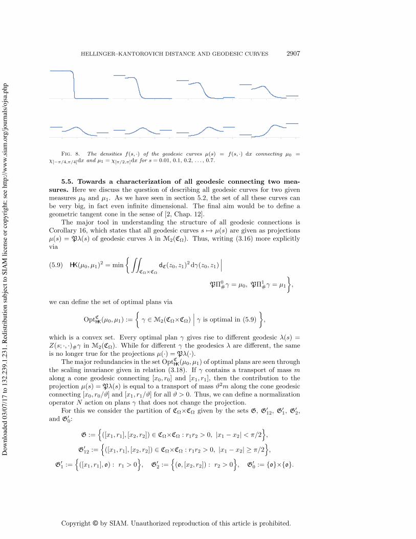
Copyright © by SIAM. Unauthorized reproduction of this article is prohibited.
HELLINGER–KANTOROVICH DISTANCE AND GEODESIC CURVES 2907
0 1 2 3 0 1 2 3 0 1 2 3 0 1 2 3
0 1 2 3 0 1 2 3 0 1 2 3 0 1 2 3
Fig. 8. The densities f(s, ·) of the geodesic curves µ(s) = f(s, ·) dx connecting µ
0
=�
[�⇡/4,⇡/4]
dx and µ
1
= �
[⇡/2,⇡]
dx for s = 0.01, 0.1, 0.2, . . . , 0.7.
5.5. Towards a characterization of all geodesic connecting two mea-sures. Here we discuss the question of describing all geodesic curves for two givenmeasures µ0 and µ1. As we have seen in section 5.2, the set of all these curves canbe very big, in fact even infinite dimensional. The final aim would be to define ageometric tangent cone in the sense of [2, Chap. 12].
The major tool in understanding the structure of all geodesic connections isCorollary 16, which states that all geodesic curves s 7! µ(s) are given as projectionsµ(s) = P�(s) of geodesic curves � in M2(C⌦). Thus, writing (3.16) more explicitlyvia
(5.9) HK(µ0, µ1)2 = min
⇢
ZZ
C⌦⇥C⌦
dC
(z0, z1)2d�(z0, z1)
�
�
�
P⇧0#� = µ0, P⇧1
#� = µ1
�
,
we can define the set of optimal plans via
OptCHK(µ0, µ1) :=
⇢
� 2 M2(C⌦⇥C⌦)�
�
�
� is optimal in (5.9)
�
,
which is a convex set. Every optimal plan � gives rise to di↵erent geodesic �(s) =Z(s; ·, ·)#� in M2(C⌦). While for di↵erent � the geodesics � are di↵erent, the sameis no longer true for the projections µ(·) = P�(·).
The major redundancies in the set OptCHK(µ0, µ1) of optimal plans are seen throughthe scaling invariance given in relation (3.18). If � contains a transport of mass malong a cone geodesic connecting [x0, r0] and [x1, r1], then the contribution to theprojection µ(s) = P�(s) is equal to a transport of mass #2m along the cone geodesicconnecting [x0, r0/#] and [x1, r1/#] for all # > 0. Thus, we can define a normalizationoperator N action on plans � that does not change the projection.
For this we consider the partition of C⌦⇥C⌦ given by the sets G, G012, G
01, G
02,
and G
00:
G :=n
([x1, r1], [x2, r2]) 2 C⌦⇥C⌦ : r1r2 > 0, |x1 � x2| < ⇡/2o
,
G
012 :=
n
([x1, r1], [x2, r2]) 2 C⌦⇥C⌦ : r1r2 > 0, |x1 � x2| � ⇡/2o
,
G
01 :=
n
([x1, r1], o) : r1 > 0o
, G
02 :=
n
(o, [x2, r2]) : r2 > 0o
, G
00 := {o}⇥{o}.
Dow
nloa
ded
03/0
7/17
to 1
32.2
39.1
.231
. Red
istri
butio
n su
bjec
t to
SIA
M li
cens
e or
cop
yrig
ht; s
ee h
ttp://
ww
w.si
am.o
rg/jo
urna
ls/o
jsa.
php
Copyright © by SIAM. Unauthorized reproduction of this article is prohibited.
2908 M. LIERO, A. MIELKE, AND G. SAVARE
With these sets we define the scaling function
#(z1, z2) :=
8
>
>
>
<
>
>
>
:
⇣
r1r2 cos(|x1 � x2|)⌘1/2
if (z1, z2) 2 G,
r1 if (z1, z2) 2 G
01,2 [G
01,
r2 if (z1, z2) 2 G
02,
1 if z1 = z2 = o
and employ the dilation map h#
from (3.17) to generate the corresponding rescalingN : M2(C⌦⇥C⌦) ! M2(C⌦⇥C⌦) by N� := (h
#
)]
(#2�) (C⌦⇥C⌦ \ G00), where de-
notes restriction of a measure. By the definition ofP and the scaling property of dC
wefirst find P⇧j
#� = P⇧j
#N� andRR
C⌦⇥C⌦dC
(z0, z1)2 d� =RR
C⌦⇥C⌦dC
(z0, z1)2 d(N�).
Hence, for each � 2 OptCHK(µ0, µ1) we again have N� 2 OptCHK(µ0, µ1). Thus, we definethe normalized optimal plans via
(5.10) NormOptCHK(µ0, µ1) :=
⇢
� 2 OptCHK(µ0, µ1)�
�
�
� = N�
�
,
which is a much smaller but still closed and convex set.Using the scaling properties of the geodesics on C⌦, which are given via the
interpolating functions Z = (X,R) as µ(s) = PZ(s; ·, ·)#� (cf. (3.21)), and the factthat # depends on x1, x2 only through their distance |x1�x2|, we also see that � andN� generate the same geodesic, namely
bµ�
(s) := P
�
Z(s; ·, ·)#)��
= P
�
Z(s; ·, ·)#(N�)�
= bµN�
(s).
With these preparations we are able to prove that there exists a unique geodesicconnecting µ0 to µ1 if µ0 is absolutely continuous with respect to the Lebesguemeasure. More precisely, we show that in this case N eliminates all redundancies:NormOptCHK(µ0, µ1) contains only one element, and N� characterize the geodesic con-nection of µ0 and µ1 uniquely.
Theorem 23. For every couple µ0, µ1 in M(⌦) with µ0 absolutely continuouswith respect to the Lebesgue measure, there exist a unique geodesic µ connecting µ0
to µ1 and a unique � 2 NormOptCHK(µ0, µ1). In particular, for each geodesic curve µconnecting µ0 to µ1 there exists a unique � 2 NormOptCHK(µ0, µ1) such that µ = bµ
�
.
Proof. By the above discussion we have to only check the uniqueness of �. Wefirst show that any � 2 NormOptCHK(µ0, µ1) does not charge G
012.
Since � is optimal, the rescaling given by N and [17, Thm. 7.21] yield that
�(G012) = �(eG0
12), where
e
G
012 =
n
([x1, 1], [x2, r2]) 2 C⌦⇥C⌦ : r2 > 0, |x1 � x2| = ⇡/2o
⇢ G
012.
Setting eµ0 := ⇧1]
(� e
G
012) = P⇧1
]
(� e
G
012), we have eµ0 = ⌘µ0 µ0; in particular,
eµ0 is absolutely continuous with respect to the Lebesgue measure. If we set f(x) :=min
y2supp(µ1) |x� y|, applying [17, Thm. 6.3(b)] we deduce that
f(x) = ⇡/2 for eµ0-a.e. x 2 ⌦.
Applying the co-area formula to f (see [9, Lem. 3.2.34], we have
L d
⇣
�
x 2 Rd⇡/2�" f(x) ⇡/2+"
⌘
=
Z
⇡/2+"
⇡/2�"
H d�1(f�1(p))dp for every " > 0,
Dow
nloa
ded
03/0
7/17
to 1
32.2
39.1
.231
. Red
istri
butio
n su
bjec
t to
SIA
M li
cens
e or
cop
yrig
ht; s
ee h
ttp://
ww
w.si
am.o
rg/jo
urna
ls/o
jsa.
php
Copyright © by SIAM. Unauthorized reproduction of this article is prohibited.
HELLINGER–KANTOROVICH DISTANCE AND GEODESIC CURVES 2909
so that passing to the limit as " # 0 we get L d
�
{x 2 Rd |f(x) = ⇡/2 }�
= 0. It followsthat eµ0 is the null measure and �(G0
12) = 0.Let us now suppose that �0, �00 2 NormOptCHK(µ0, µ1).Combining Theorems 7.2.1(iv) and 6.7 of [17] (where we use the absolute continu-
ity of µ0 again) we see that the restrictions of �0 and �00 to G coincide. By subtractingthis common part from both of them and the corresponding homogeneous marginalsfrom µ0 and µ1, it is not restrictive to assume that �0 and �00 are concentrated in thecomplement of G. By the previous claim, we obtain that �0 and �00 are concentratedon G
01 [G
02.
It is also easy to see that the restrictions of �0 and �00 to G
i
, i = 1, 2, coincideas well: considering, e.g., G0
1, by construction we have that ⇧1]
�0 = ⇧1]
�00 = µ1 ⌦ �1,
whereas ⇧2]
�0 = ⇧2]
�00 = µ1(Rd)�o
. It follows that �0 G
01 = �00 G
01 = (µ1 ⌦ �1)⌦ �
o
.A similar argument holds for G0
2. This proves the result.
The major point in the above proof is to show that ��
e
G
012
�
= 0, i.e., there is notransport over the distance ⇡/2. From section 5.2 we know that in the opposite caseNormOptCHK(µ0, µ1) can be infinite dimensional.
We expect that, by refining the arguments above and using the dual character-ization of HK, it is possible to prove that for each geodesic curve connecting µ0 andµ1 (both not necessarily absolutely continuous with respect to L d) there exists aunique � 2 NormOptCHK(µ0, µ1) such that µ = bµ
�
. As in the Kantorovich–Wassersteincase, the optimal plan � should be uniquely determined by fixing an intermediatepoint bµ
�
(s) with s 2 ]0, 1[ along a geodesic. In particular, geodesics for the Hellinger–Kantorovich distance HK in M(⌦) will then be nonbranching. Indeed, for the rich setof geodesics connecting two Dirac masses at distance ⇡/2 discussed in section 5.2 thiscan be shown by direct inspection. We will address these questions in a forthcomingpaper.
5.6. HK is not globally semiconcave. The metric on a geodesic space (Y, d)is called K-semiconcave if for all points y0, y1, y⇤ 2 Y and all minimal geodesic curvesey : [0, 1] ! Y with ey(i) = y
i
for i 2 {0, 1} we have
(5.11) d(ey(s), y⇤)2 � (1�s)d(y0, y⇤)
2 + sd(y1, y⇤)2 �Ks(1�s)d(y0, y1)
2.
It is well known that the Wasserstein distance on a domain ⌦ ⇢ Rd is 1-semiconcave(such that (P2(⌦),W) is a PC space; see [2, Chap. 12.3]), and it is easy to checkthat the Hellinger–Kakutani distance H is 1-semiconcave. Indeed, with the notationof section 2.3 we have the identity
H(µH(s), µ⇤)2 = (1�s)H(µ0, µ⇤)
2 + sH(µ1, µ⇤)2 � s(1�s)H(µ0, µ1)
2
for any µ0, µ1, µ⇤ 2 M(⌦), where s 7! µH(s) 2 M(⌦) is the Hellinger geodesic from(2.8).
In contrast, the Hellinger–Kantorovich distance is not K-semiconcave for any Kif ⌦ is not one dimensional. For the one-dimensional case ⌦ ⇢ R it is shown in [17,Thm. 8.9] that (M([a, b]),HK) is a PC space, which means that 1-semiconcavity holds.The following result shows that (M(⌦),HK) is not a PC space if ⌦ has dimensiond � 2.
For this case we consider a simple example, namely
µ0 = �x0, µ1 = �
x1, µ⇤ = b�
z
, with x0 = 0, x1 = ⇡
2 e1, z = ⇡
4 e1 + ye2,
Dow
nloa
ded
03/0
7/17
to 1
32.2
39.1
.231
. Red
istri
butio
n su
bjec
t to
SIA
M li
cens
e or
cop
yrig
ht; s
ee h
ttp://
ww
w.si
am.o
rg/jo
urna
ls/o
jsa.
php

Copyright © by SIAM. Unauthorized reproduction of this article is prohibited.
2910 M. LIERO, A. MIELKE, AND G. SAVARE
where e1 and e2 are the first two unit vectors and y > 0. As a geodesic curve wechoose
µ(s) = a(s)�⇢(s)e1 with a(s) = (1�s)2 + s2 and ⇢(s) = arctan(s/(1�s)).
We have HK(µ0, µ1)2 = 2 and µ(1/2) = 12�⇡
4 e1, and all the quantities in the semicon-
cavity condition (5.11) can be evaluated explicitly. This yields a lower bound for K,namely
K �12HK(µ0, µ⇤)2 +
12HK(µ1, µ⇤)2 � HK(µ( 12 ), µ⇤)2
14HK(µ0, µ1)2
= 1 +pb �(y) with �(y) =
p8 cos
⇡/2(y)� 4 cos⇡/2
p
y2 + ⇡2/16,
where cos⇡/2 a = cos
�
min{|a|,⇡/2}�
. Since �(y) > 0 for y 2 ]0,p3⇡/4[ and since b
can be chosen arbitrarily large, we see that there cannot exist a finite K such that HKis K-semiconcave on all of M(⌦).
REFERENCES
[1] S. Adams, N. Dirr, M. A. Peletier, and J. Zimmer, From a large-deviations principle to theWasserstein gradient flow: A new micro-macro passage, Comm. Math. Phys., 307 (2011),pp. 791–815, doi:10.1007/s00220-011-1328-4.
[2] L. Ambrosio, N. Gigli, and G. Savare, Gradient Flows in Metric Spaces and in the Spaceof Probability Measures, Lectures Math. ETH Zurich, Birkhauser Verlag, Basel, 2005.
[3] J.-D. Benamou and Y. Brenier, A computational fluid mechanics solution to the Monge-Kantorovich mass transfer problem, Numer. Math., 84 (2000), pp. 375–393, doi:10.1007/s002110050002.
[4] D. Burago, Y. Burago, and S. Ivanov, A Course in Metric Geometry, Grad. Stud. Math.33, American Mathematical Society, Providence, RI, 2001.
[5] L. Chayes and H.-K. Lei, Optimal Transport for Non-conservative Systems, preprint, arXiv:1410.3923, 2014.
[6] L. Chizat, G. Peyre, B. Schmitzer, and F.-X. Vialard, An Interpolating Distance betweenOptimal Transport and Fisher–Rao, preprint, arXiv:1506.06430v2, 2015; Found. Comput.Math., to appear.
[7] L. Chizat, G. Peyre, B. Schmitzer, and F.-X. Vialard, Unbalanced Optimal Transport:Geometry and Kantorovich Formulation, preprint, arXiv:1508.05216v1, 2015.
[8] S. Daneri and G. Savare, Eulerian calculus for the displacement convexity in the Wassersteindistance, SIAM J. Math. Anal., 40 (2008), pp. 1104–1122, doi:10.1137/08071346X.
[9] H. Federer, Geometric Measure Theory, Springer-Verlag, New York, 1969.[10] E. Hellinger, Neue Begrundung der Theorie quadratischer Formen von unendlichvielen
Veranderlichen, J. Reine Angew. Math., 136 (1909), pp. 210–271, doi: 10.1515/crll.1909.136.210.
[11] R. Jordan, D. Kinderlehrer, and F. Otto, Free energy and the Fokker-Planck equation,Phys. D, 107 (1997), pp. 265–271, doi:10.1016/S0167-2789(97)00093-6.
[12] R. Jordan, D. Kinderlehrer, and F. Otto, The variational formulation of theFokker-Planck equation, SIAM J. Math. Anal., 29 (1998), pp. 1–17, doi:10.1137/S0036141096303359.
[13] S. Kakutani, On equivalence of infinite product measures, Ann. of Math. (2), 49 (1948),pp. 214–224, doi:10.2307/1969123.
[14] S. Kondratyev, L. Monsaingeon, and D. Vorotnikov, A New Optimal Transport Distanceon the Space of Finite Radon Measures, preprint, arXiv:1505.07746v2, 2015.
[15] M. Liero and A. Mielke, Gradient structures and geodesic convexity for reaction-di↵usionsystems, Philos. Trans. R. Soc. Lond. Ser. A Math. Phys. Eng. Sci., 371 (2013), 20120346,doi:10.1098/rsta.2012.0346.
[16] M. Liero, A. Mielke, and G. Savare, Geodesic �-Convexity for the Hellinger–KantorovichDistance, manuscript, 2016.
[17] M. Liero, A. Mielke, and G. Savare, Optimal Entropy-Transport Problems and theHellinger–Kantorovich Distance, preprint, arXiv:1508.07941v1, 2015, WIAS preprint 2207,submitted.
Dow
nloa
ded
03/0
7/17
to 1
32.2
39.1
.231
. Red
istri
butio
n su
bjec
t to
SIA
M li
cens
e or
cop
yrig
ht; s
ee h
ttp://
ww
w.si
am.o
rg/jo
urna
ls/o
jsa.
php

Copyright © by SIAM. Unauthorized reproduction of this article is prohibited.
HELLINGER–KANTOROVICH DISTANCE AND GEODESIC CURVES 2911
[18] S. Lisini, Characterization of absolutely continuous curves in Wasserstein spaces, Calc. Var.Partial Di↵erential Equations, 28 (2007), pp. 85–120, doi:10.1007/s00526-006-0032-2.
[19] S. Maniglia, Probabilistic representation and uniqueness results for measure-valued solutionsof transport equations, J. Math. Pures Appl. (9), 87 (2007), pp. 601–626, doi:10.1016/j.matpur.2007.04.001.
[20] A. Mielke, A gradient structure for reaction-di↵usion systems and for energy-drift-di↵usionsystems, Nonlinearity, 24 (2011), pp. 1329–1346, doi:10.1088/0951-7715/24/4/016.
[21] A. Mielke, Thermomechanical modeling of energy-reaction-di↵usion systems, including bulk-interface interactions, Discrete Contin. Dyn. Syst. Ser. S, 6 (2013), pp. 479–499, doi:10.3934/dcdss.2013.6.479.
[22] L. Onsager, Reciprocal relations in irreversible processes, II, Phys. Rev., 38 (1931), pp. 2265–2279, doi:10.1103/PhysRev.38.2265.
[23] L. Onsager and S. Machlup, Fluctuations and irreversible processes, Phys. Rev., 91 (1953),pp. 1505–1512, doi:10.1103/PhysRev.91.1505.
[24] F. Otto, Dynamics of labyrinthine pattern formation in magnetic fluids: A mean-field theory,Arch. Rational Mech. Anal., 141 (1998), pp. 63–103, doi:10.1007/s002050050073.
[25] F. Otto, The geometry of dissipative evolution equations: The porous medium equa-tion, Comm. Partial Di↵erential Equations, 26 (2001), pp. 101–174, doi:10.1081/PDE-100002243.
[26] F. Otto and M. Westdickenberg, Eulerian calculus for the contraction in the Wassersteindistance, SIAM J. Math. Anal., 37:4 (2005), pp. 1227–1255, doi:10.1137/050622420.
[27] B. Perthame, F. Quiros, and J. L. Vazquez, The Hele-Shaw asymptotics for mechani-cal models of tumor growth, Arch. Rational Mech. Anal., 212 (2014), pp. 93–127, doi:10.1007/s00205-013-0704-y.
[28] A. Schied, Sample path large deviations for super-brownian motion, Probab. Theory RelatedFields, 104 (1996), pp. 319–347, doi:10.1007/BF01213684.
[29] C. Villani, Optimal Transport. Old and New, Springer, Berlin, 2009, doi:10.1007/978-3-540-71050-9.
Dow
nloa
ded
03/0
7/17
to 1
32.2
39.1
.231
. Red
istri
butio
n su
bjec
t to
SIA
M li
cens
e or
cop
yrig
ht; s
ee h
ttp://
ww
w.si
am.o
rg/jo
urna
ls/o
jsa.
php