1

The John R Smith Sky Survey at 408 MHz

John Smith, Phil Beastall, Brian Shorter, Sally Smith, Ken Tapping, Dave Vincent, Chip Wiest, James Wilhelm

Dedication: The survey described here is dedicated to John R. Smith, who played the leading role in the decision to do this survey, and in the design and construction of the 30ft dish intended to make it. He provided leadership, developed hardware, electronics and software and started the observing programme. John played a key role in the success of amateur radio astronomy in the UK and helped it spread to Canada and other countries. Unfortunately, his untimely death meant he was not to see the results of what he started. This survey is also dedicated to the memory of Sally, John’s daughter, who worked very hard to see the survey completed, and lived just long enough to see it achieved.

23.31

23.11

22.91

22.71

22.51

22.31

22.11

21.91

21.71

21.51

21.21

21.01

20.81

20.61

20.41

20.21

20.01

19.81

19.61

19.41

19.21

19.01

18.81

18.61

18.41

18.21

18.01

17.81

17.61

17.41

17.21

11

13

15

17

19

21

23

25

27

29

31

33

35

37

39

S31

S33

S35

S37

S39

Right Ascension in Hours

Dec

linat

ioni

n D

egre

es

Summer Night Sky at 408 MHz

90-95

85-90

80-85

75-80

70-75

65-70

60-65

55-60

50-55

45-50

40-45

35-40

30-35

25-30

20-25

15-20

10-15

5-10

0-5

Figure 1: The Summer Night Milky Way at 408 MHz. The two bright patches towards the top of the map are due to the radio sources Cygnus A (right) and Cygnus X (left). The units are antenna temperature in Kelvins.

2

1. Introduction Figures 1 and 2 show maps of the sky between declination 0 and 50 degrees North, made using the 30ft radio telescope located at Ellen’s Green, near Cranleigh, UK, at a frequency of 408 MHz. It shows radio emission from our galaxy, the Milky Way, together with a few of the brighter discrete radio sources. The terms winter and summer Milky Way might seem strange for radio observations. However, due to solar interference, the best radio observations were mainly made at night, which brought the observations into a similar situation to that in optical astronomy, and during the survey, the terminology just stuck. The sensitivity of the radio telescope is better than shown in these maps. However, the data selection process for this iteration in map preparation has been rather conservative.

The first radio sky surveys were done by Grote Reber, at 160 MHz and 480 MHz, in the 1940’s. Two interesting aspects of Reber’s work of more than 60 years ago relevant to this survey are firstly, that Reber’s radio telescope was a 32-ft dish, which is almost the same size as the 30-ft dish used here. The second is that Reber managed to do his survey from a suburban location at Wheaton, Illinois, where although interference was sometimes objectionable, it never stopped him observing. This survey was made from a country location, but over the decades since Reber made his surveys, the situation with manmade interference has become very much worse. If Reber were trying to do his surveys these days, his receiving system would be overwhelmed by the interference. Without having better electronics and the use of computers for data sorting and processing, the survey would have been impossible.

1.61

2.01

2.41

2.81

3.21

3.61

4.01

4.41

4.81

5.21

5.61

6.01

6.41

6.81

7.21

7.61

8.01

8.41

8.81

9.21

9.61

10.01

10.41

10.81

11.21

11.61

11

1417

2023262932353841

444750

Right Ascension in Hours

Declination in D

egrees

Winter Night Sky at 408 MHz

16-18

14-16

12-14

10-12

8-10

6-8

4-6

2-4

0-2

3

Sky Surveys are difficult. They make demands on the environment and equipment that are far fiercer than those encountered in other branches of radio astronomy. The most stringent needs are for the radio telescope system to be extremely stable, and the interference environment to be tolerable for long periods of time. In the instance discussed here, these needs were marginally met. The radio telescope used was the 30ft alt-az paraboloid built by John Smith and Ken Tapping, and currently located near Cranleigh, Surrey, UK. The instrument and the survey are discussed in detail in the following sections.

2. The 30ft Radio Telescope: A Short History

Figure 3: The 30ft Dish as currently operating near Cranleigh. The azimuth track is hidden in the grass. The feed and focus box are as used in the survey. The 30ft paraboloidal radio telescope, currently located at Ellen’s Green, near Cranleigh, is a circular mesh dish on an altazimuth mount. Although it is possible to control the antenna using a computer, for the purposes of this project, all the driving was done manually. The dish is shown in Figure 3. The dish rotates in azimuth on a circular track, driven by electric motors on the front two corners and on undriven wheels on the rear corners. To keep the structure as low as possible, the declination axis is located a few feet from the front edge. The dish can be tilted forward, from its vertical-facing, rest position, when the dish is sitting in its frame, until the front lip of the dish touches the ground,

4

which is roughly declination zero degrees – the celestial equator – when the telescope is pointed south. The big disadvantage of this design approach is the large amount of counterweight needed. However, this is more than balanced by the greater accessibility to the main structural elements without ladders.

The elevation drive consists of a motor driving a turnbuckle via an old washing machine gearbox. The shortening turnbuckle pulls a wheel along the track mounted on the centre member of the dish frame. The wheel is in turn attached to two pipes, which push the rear of the dish up. Position indication is obtained via synchros attached to the elevation and azimuth axes.

The idea for building the dish arose in the late 1960’s when John Smith and his family lived near Halstead, in Kent. John had a long history in amateur radio astronomy, having built a number of instruments of various sizes, and used them for successfully observing a number of sources, and for running many years of systematic observations of solar radio emissions. Around that time, Ken Tapping was a relative beginner in radio astronomy, and John and Ken spent a lot of time trying various experiments. One of the things that were often discussed was the idea of doing a sky survey. Shortly before that time, John had built a 20ft dish, but had not mounted it. However, before that happened, a windstorm badly damaged it. After looking at it, Ken and John decided that the work of salvaging the dish would be more than building another from scratch. Then, John said “Why should we build another 20ft dish? A 30ft dish sounds more useful.” Since the other radio telescopes were called the Mk. 1 (a 140 MHz phase switched interferometer using two small paraboloic cylinders, used mainly for observing the Sun), the Mk. 2 (a large, 60 x 10 ft parabolic cylinder), and the Mk. 3 (the 20 ft dish mentioned above), the 30 ft dish became known as the Mk 4.

Since there was a metal yard quite close by that sold steel strip, girders and angle for very reasonable prices, this dish would be all metal. Although John and Ken would share the work and the cost, Ken points out that John was by far the brains behind the dish construction project. At first it was intended to bolt the whole thing together, but then, by combining an old motorcycle engine with a dynamo, John made an electric welder. This was used for the construction of the dish surface. The geodetic concept of making the dish surface out of triangles was used in order to maximize the structural strength of the surface, and so reduce the need for backing structure. The surface chicken wire with a half-inch mesh. The focal length of the dish was set to be 15ft, so that when the focal assembly was lowered, it would sit on the dish edge. With the dish tilted, this made working on the receiver very easy.

Thanks to additional help from other local amateur radio astronomers, including Gordon Brown and Michael Hale, in 1971 the dish was ready for testing. There was at that time no receiver for it, so a 136 MHz receiver Ken had built for his own experiments was installed on the dish. It was clear that the radio telescope was working, but it was also clear that the dish was not working properly. To have problems with using a 9-m dish at a wavelength of 2.2 m, there had to be something seriously wrong somewhere. However, getting to grips with the problem was stopped by another blow, which actually proved to be a blessing in disguise. John’s job had been transferred to Guildford. The Smiths would be moving, and the dish had to come apart again. To see the results of a lot of work be

5

again reduced to piles of parts was heartbreaking, as was the sight of this “home radio telescope kit” sitting on the ground at the new site, just outside Cranleigh, Surrey.

Thanks to that “practice run” at Halstead, putting everything back together didn’t take as long as feared. Using a water gauge and tape measure to get the antenna into the right shape, we found some serious dish surface errors; these were fixed. When the telescope was complete, we built a 408 MHz Dicke receiver to use on it. During these tests, made trying various types of receiver, the dish worked well, and some excellent recordings of the Crab Nebula and IC443 were obtained. At this point there seemed to be no hurry to start, so John and Ken had a lot of fun trying different designs for feeds and receivers. One of the experiments was to record high-speed pulsations in solar radio emissions. The next blow came in 1975, when Ken accepted a job in Canada, intending to work there for a few years. This slowed the work considerably, but over the next few years John used the dish for a number of projects, but not the long-planned sky survey.

With 1989 came yet another blow. It became necessary to move the radio telescope again, which John achieved single-handed, and the dish was reassembled at its current site near Ellen’s Green. In 1997 Ken’s trips to the UK became fairly frequent, and momentum built up in getting seriously ready for the long period of careful observations that would be involved in making the survey. Then, in 1998, John died. The project could very well have ended then. However, we, and in particular John’s daughter Sally, felt that after all this work, particularly by John, the survey should be completed. In recognition of John’s primary role in the project, and his long-standing contribution to amateur radio astronomy, the survey is dedicated to him.

3. Sky Surveys: Problems, Ideas and Solutions A radio sky survey consists of mapping the distribution of various properties of radio emission over the sky. These properties can include: intensity, polarization, spectrum, and perhaps time variability. The instruments can be similarly diverse. Interferometers are best for the detection of small sources and mapping of small angular structures, but for general purpose mapping, the best general purpose survey instrument is a large, paraboloidal antenna, perhaps in combination with an interferometer. This would provide both the capability of mapping large, diffuse, faint emission covering large areas of sky, like the galactic emission, together with the ability to detect and identify sources of small angular diameter. In this project, a single large (at least by amateur standards) paraboloid was used, so the subsequent discussion is aimed mainly in that direction.

A single-antenna radio telescope is the radio analogue of a large lens or mirror with a photocell at the focus. To make an image the radio brightness of the sky has to be observed point by point. The most straightforward is to divide the sky to be mapped into a two-dimensional grid of points, and then measure those points one by one. An alternative that is almost as good is to point the telescope at the meridian, and then scan north and south as the rotation of the Earth carries the sky past. These are the two preferred methods, but they both require an antenna that is automated and precisely controllable. We decided two use a third, less efficient method, namely to point the antenna at the declination of interest, on the meridian, and allow the rotation of the Earth to move the sky through the antenna beam. In that way, by changing the declination and

6

repeating the process the sky is scanned, strip by strip. Although more time intensive, this method has two great advantages: firstly the antenna is pointed by hand to the required declination, and then held at that position, avoiding problems with precise control and automation. Secondly, during the observation, the antenna remains fixed with respect to the ground, so it always receives the same amount of ground radiation. The downside is that with observations being made over very long periods, receiver stability now becomes a very major issue.

4. Theory Assume we have a radio telescope with an antenna having a gain G0 in the boresight direction (the intended viewing direction), and pointing in the direction azimuth φ and elevation θ. The output of the receiver, when looking at broad-band cosmic noise, is actually the sum of a number of contributions, most of which are unwanted.

( )mosskyGRout TTTTTP cosint ++++Γ∝

where:

• Γ is the gain-bandwidth product of the receiver. Since cosmic signals are weak, a lot of amplification is needed. The receiver used in this project has a total (gross) amplification of about 120dB and a bandwidth of roughly 2 MHz;

• TR is the system noise temperature of the receiver system, including the antenna components. In this case, the front-end amplifier has a noise temperature of less than 50 K. However, taking into account the insertion loss of the additional components between the amplifier input and the antenna feed, the overall value is probably more like 120 K.

• TG is the amount of noise radiated by the ground and picked up by the antenna when looking at elevation θ. All objects in the universe that have a temperature radiate radio waves. The ground is a brighter radio source than most of the sources in the sky. There is no such thing as an antenna that receives only radio waves coming from a given direction. All antennas have some sensitivity to radio waves coming from any direction. The big trick in radio telescope design is to minimize the sensitivity of the antenna to signals and noise arriving from directions outside the main beam of antenna. The biggest single issue is “spillover”, where the feed at the focus of the antenna, which picks up the energy collected by it, “sees” energy coming from directions beyond the edge of the dish. This provides sensitivity to interference coming from behind the dish, and no matter elevation to which the antenna is set, picks up thermal noise from the ground. Consequently, this “ground noise” is always there, for all radio telescopes. The shape of the antenna sensitivity pattern makes the ground noise picked up by an antenna vary strongly with elevation, and not always in an intuitive way.

• Tsky is the noise received mainly from the troposphere and the ionosphere. At wavelengths of centimetres or shorter, the troposphere is a major source of

7

attenuation and noise, at longer wavelengths, the ionosphere becomes more important. When the antenna is looking at low elevations, it is looking through more atmosphere, so that this contribution is also strongly variable with elevation, and possibly with antenna azimuth.

• In an era where there is an increasing number of radio services scrambling for space in the radio spectrum, interference is becoming more of a problem for radio astronomy, and is expected to get worse. Interference might be very strong, but one or two weak interferers can make the receiver output vary irregularly and make data analysis very difficult, or impossible. Even though it is not technically correct to do so, we describe the interference level also as a temperature, Tint. This quantity can be a function of antenna pointing direction and time.

• Lastly we come to the quantity we wish to measure. Tcosmos is the average brightness of the radio emission over the patch of sky seen by the radio telescope.

The other noise contributions led to our decision to make the map by setting the antenna to a specified declination on the southern meridian (hour angle = 0), and letting the sky move through the antenna beam. In this way the antenna elevation remained constant, so that the effect of ground and sky noise would be a constant offset (which can be eliminated) rather than something varying in a way that would lead to its being confused with cosmic radio emission. In addition, any weak, distant sources of interference might produce a reasonably constant output from the radio receiver.

If a constant input is provided to a radio telescope receiver, the output will inevitably drift. This is due to variations in the receiver gain. If the total of the receiver, ground and sky noise contributions is around 200 K, and the radio source increases the antenna temperature by 1 K, then a change in receiver gain of less than 0.5 % will produce a change in receiver output equal to the change produced by the source. Such gain drift happens over many timescales, depending upon the receiver design, stability of the power supplies, variations in ambient temperature etc., but typically it can vary over timescales ranging from fractions of a second to hours. Although the focus box had its temperature regulated, the rest of the receiver was in an unheated, uninsulated shed. The short-term variations were minimized through the use of a Dicke switching receiver design, and the slower variations through frequent addition of a fixed calibration signal.

One consistent source of interference was the Sun. Our nearest star is a strong radio source, and an interesting subject for amateur radio astronomers because it is bright, and produces a fascinating menagerie of radio emissions. A bright, moving source of varying radio emissions is very undesirable when surveys are being done, and there is no easy way to deal with it. Therefore, on most days, particularly when the Sun was exceptionally active, useful observations could only be done at night.

5. The Equipment

5.1 The Antenna The antenna is a 30ft mesh dish with an altazimuth mount. The cosmic signals are collected using a feed mounted at the focus of the dish. The feed is supported on a bipod

8

that is mounted so that it pivots in the elevation plane, and is kept in place using two guy ropes in a plane perpendicular to that of the bipod. Access to the feed is obtained by tilting the dish until the lip is 3-4ft from the ground, and then lowering the feed by slackening off one of the guy ropes until it is almost resting on the edge of the dish. To reduce the effort in handling the bipod when it was almost lowered, and to make it more controllable, a flying jib arrangement was used.

The feed is a dipole and reflector mounted within a cavity fabricated from a sheet of galvanized steel. The receiver is mounted in a focus box mounted directly behind the feed assembly.

The half-power beamwidth of the dish is about 5 degrees.

To compare the real antenna with what we thought it should be, we used a simple radiator model to estimate the beam pattern. An imaginary transmitter located at the feed position illuminated a grid of close-spaced imaginary nodes on the dish surface. These were assumed to reradiate the signal in all directions, with the amplitude and phase of the signal unchanged. Then, at a distant point, the vector signals from all the nodes were summed. The beam pattern was calculated by varying the angular offsets of the measurement point from the antenna boresight. We used this method to investigate the effects of offsets of the feed from the focus position. It also showed a sidelobe asymmetry to be due to one edge of the dish being about an inch lower than the other. Observations of isolated bright sources, such as Cassiopeia A confirm that the antenna beamwidth is indeed 5 degrees.

5.2 The Receiver The receiver is a fairly standard Dicke design. Its main features are shown in the block diagram below:

Focus Box

Input from Feed

DirectionalCoupler

Noise Source

Low-Noise GaAsFET Amplifier

Attenuator

GaAsFET Amplifier

Cable to rest of receiver

Dicke Switch

Square Wave Drive From Signal Processor

Control Signal from Signal Processor

9

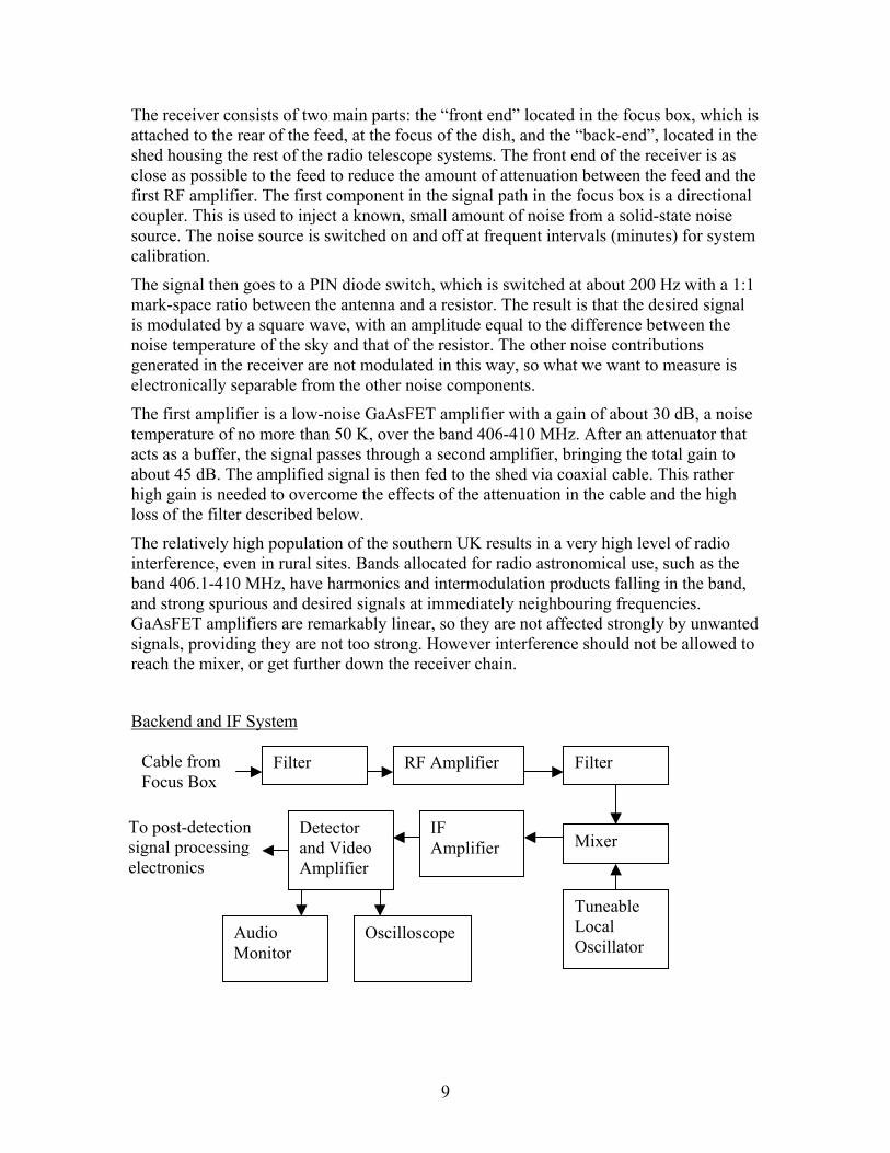
The receiver consists of two main parts: the “front end” located in the focus box, which is attached to the rear of the feed, at the focus of the dish, and the “back-end”, located in the shed housing the rest of the radio telescope systems. The front end of the receiver is as close as possible to the feed to reduce the amount of attenuation between the feed and the first RF amplifier. The first component in the signal path in the focus box is a directional coupler. This is used to inject a known, small amount of noise from a solid-state noise source. The noise source is switched on and off at frequent intervals (minutes) for system calibration.

The signal then goes to a PIN diode switch, which is switched at about 200 Hz with a 1:1 mark-space ratio between the antenna and a resistor. The result is that the desired signal is modulated by a square wave, with an amplitude equal to the difference between the noise temperature of the sky and that of the resistor. The other noise contributions generated in the receiver are not modulated in this way, so what we want to measure is electronically separable from the other noise components.

The first amplifier is a low-noise GaAsFET amplifier with a gain of about 30 dB, a noise temperature of no more than 50 K, over the band 406-410 MHz. After an attenuator that acts as a buffer, the signal passes through a second amplifier, bringing the total gain to about 45 dB. The amplified signal is then fed to the shed via coaxial cable. This rather high gain is needed to overcome the effects of the attenuation in the cable and the high loss of the filter described below.

The relatively high population of the southern UK results in a very high level of radio interference, even in rural sites. Bands allocated for radio astronomical use, such as the band 406.1-410 MHz, have harmonics and intermodulation products falling in the band, and strong spurious and desired signals at immediately neighbouring frequencies. GaAsFET amplifiers are remarkably linear, so they are not affected strongly by unwanted signals, providing they are not too strong. However interference should not be allowed to reach the mixer, or get further down the receiver chain.

Backend and IF System

Filter Cable from Focus Box

IF Amplifier

Tuneable Local Oscillator

Filter

Detector and Video Amplifier

Mixer

RF Amplifier

To post-detection signal processing electronics

OscilloscopeAudio Monitor

10

Upon arrival in the shed, the received signal is passed through a combination of filters, including a multipole interdigital filter and a quarter-wave coaxial line filter before being passed to the mixer, which is a commercial double-balanced design. The local oscillator is tuneable, so that strong interference can be avoided. The output from the mixer is fed to the main IF amplifier, which has a variable gain, between 60 and 90 dB, at a centre frequency of 30 MHz. Its bandwidth is about 1 MHz. It has a built in detector and video amplifier. The video amplifier has a frequency response extending to below 200 Hz, so it fulfils two useful purposes: it amplifies the signal we wish to measure and being AC coupled, it rejects all the DC voltages from the demodulated receiver noise components. The output from the amplifier is fed to the signal processor, and for monitoring purposes, to an oscilloscope and audio monitor.

4.3 The Signal Processing System

The signal processing system is fairly conventional. The signal from the video amplifier output is AC coupled, so there are no DC components. There is simply noise plus a square wave having an amplitude proportional to the difference between the antenna temperature and the temperature of the reference load. To reduce dynamic range requirements, it is fairly common to pass the video through a band-pass filter that passes the fundamental and maybe the lower harmonics of the square wave frequency. There was no need in our case, so the LF amplifier is a standard audio-frequency amplifier, passing frequencies up to at least a few kHz. The synchronous detector is really a synchronous inverter, so that the negative parts of the square wave are inverted, and the output a DC proportional to the TA-TREF.

The DC amplifier fulfils a number of functions. It amplifiers the voltage from the synchronous detector in order to best suit the input needs of the analogue/digital converter, applies a voltage offset to place the signal in a suitable part of the A/D input voltage range, and applies a low-pass filter to the voltage to suit the sampling rate. The gain, offset and time constant are adjustable.

Low-Frequency Amplifier

Synchronous Detector

DC Amplifier/ Integrator

To Computer A/D Input

Square Wave Generator

Input from IF Video o/p

Drive to Dicke Switch in Focus Box

Logging Computer

Control Signal to Noise Source

11

5.4 Data Logging and Control This system fulfils three main functions. It logs the receiver output in an appropriate form for further processing, tagging the data with time marks, regularly turns a calibration source on and off for checks of system gain stability, and provides a “quick look display of the data and the system. For most of the survey work, a BBC microcomputer was used to accomplish these functions. For those not familiar with the BBC microcomputer, it is very similar to the Apple II+ of the late 1970s but with a number of significant enhancements – larger memory, enhanced display capabilities, built in A/D converters, parallel digital I/O etc. The BBC system worked well beyond the end of its intended lifetime. It was finally replaced with a rather more modern Windows PC system in 2004.

The BBC software was written in the dialect of BASIC that came with the machine. After a brief initialization section the program sets up a number of counters and timers that are polled in a free running loop (interrupts were not used). Readings are taken as fast as the modest processor would allow until a count of 2000 was reached or the timer satisfied. At this point an average is calculated and logged in binary form. 1200 points per day were captured (one data point every 72 seconds). The time the log started is recorded in a short 40-byte header section and the time for any given point is simply a count of the number of points logged since that time. The result was a very compact data file; well within the BBC computer’s capacity to record for a week.

All the data analysis was done on PC’s by team members scattered around the world. The first problem was to get the data from BBC format to PC format and then to distribute it. To do this the data was conveyed by “sneaker net” to a second BBC microcomputer, which was interfaced to a PC. Files could then be taken from the BBC discs and converted to Excel comma separated variable files, which could be further processed. The software for this was developed by team members.

Since few amateur radio astronomers can pick especially low interference environments, interference is a major issue, as it was in this case too. Southern England, under a flight path into Gatwick Airport is not an ideal place for doing a 408 MHz Sky Survey. Then there was also the problem of solar interference. Sorting out the usable data in an efficient fashion required additional tools, including a visual data display and editor that displayed the data and enabled one to cut out the sections worthy of further analysis.

The work of moving data from one platform to another and the distributing it, in addition to managing the observations, was excessively tedious, and we decided to replace the BBC microcomputer with a more modern but still old Windows 486 system that still seemed to have some life in it. The analogue to digital converter is an elegantly simple device by Ocean Systems based on the MAX186 a/d converter chip. The new program in concept is very much like John’s original – timers and counting loops, no interrupt handling, free running – there is a real time display, data logging and calibration control.

There are a few major changes. Rather than a separate observers’ log, the program stores its run time parameters in a header section in the logging file. The sample period is now 2 seconds and every point logged carries a time stamp. The output file is in a text format ready to load into a spreadsheet or database. However there is a price for these improvements. A daily file runs about one megabyte (raw data is no longer e-mailed but posted on a specially set up internet site for survey members). Time resolution is

12

enhanced but a lot more post processing is now required. The revised program works in a DOS, Windows 95, 98 or 98se but not in the latest operating systems.

6. Observing Techniques The observing procedure for the survey consists of setting the antenna on the meridian to the declination required, and allowing the Earth’s rotation to scan a strip of sky at that declination. Repeated observations are allowed to accumulate over a week or so. The antenna declination is then changed and the process repeated. This survey process is very slow, but allows opportunities for sorting out the good scans from those with too much interference, and identifying observations that need to be repeated. Since the antenna cannot scan northward past the zenith, the higher declinations are observed by rotating the dish 180 degrees.

Each scan will have a baseline offset related to the amount of ground radiation picked up by the antenna at that declination. Since this varies as a function of declination, it is an impediment to integrating the scans into a map

7. Data and Data Analysis The data for each declination consists of a table of receiver output versus sidereal time, with indications as to when the calibration source is turned on. The first step is to examine the scans and select those that look analysable. In many cases there were no entirely usable scans, forcing us to concoct composite scans out of fragments. The process is illustrated below. The first figure shows the scan across the Milky Way at about Dec +40 that has been built from parts of three incomplete scans. The plotted sample units are equivalent to 10 A/D units.

Basic Data

0

20

40

60

80

100

120

140

160

0 200 400 600 800 1000 1200

Sample Number

Sam

ple

Uni

ts

Figure 4: A raw scan, made from fragments, with the calibration signals removed. It suffers from interference, gain drifts and gain/offset steps.

13

Using the file of calibration signals and treating the lowest value in the scan as zero, it is possible to compensate for the gain variations. The level corresponding to “zero sky” is subtracted from all the data, and all the values are divided by the amplitude of the interpolated calibration values. The resulting gain compensated scan is shown below.

With a beamwidth of about 5 degrees, little can change in the output from the receiver in less than a minute or two, with the exception of solar flares, which would be regarded as interference in this investigation. Anything changing rapidly is not part of the data we want, so it is easy to scan the data file looking for transients.

Gain Compensated

0

20

40

60

80

100

120

0 200 400 600 800 1000 1200

Sample Number

Sam

ple

Uni

ts

Figure 5: The gain variations have been removed, but there are still steps and interference.

Steps

-60

-40

-20

0

20

40

60

80

0 200 400 600 800 1000 1200

Sample Number

Sam

ple

Uni

ts

Figure 6 : Transient changes in the receiver output as identified by software.

14

Subtracting the transients from the record produces a usable scan for incorporation into the map.

The small remaining glitches are most easily removed by hand. Although badly broken up, this scan contained enough usable data for a basis for the analysis to be estimated. If there are only short segments, analysis is impossible unless these fragments can be added together to make a scan, which will look fragmented and non-uniformly calibrated, like the one in Figure 4. Provided that a workable estimate of the cold sky, zero level can be established, jigsaw puzzle scans can be processed.

8. Building the Maps After the scans were processed, they are added to a large Excel spreadsheet with a right ascension column on the left side and a separate column for each declination surveyed. At this point each scan has some internal consistency and is more or less calibrated, when these are combined into a single map, it is apparent that there is only limited consistency between scans. These are due to a number of factors: the estimated zero levels differ between scans, which also introduces small calibration errors, there could still be interference in there somewhere, and the ground radiation contribution varies with antenna elevation. Part of it gets eliminated through the choice of zero baseline, but not all. The result is recognisable as a map, but there is clearly a lot of processing to be done. This initial map is shown in Figure 8.

Corrected Scan

0

5

10

15

20

25

30

35

40

0 200 400 600 800 1000 1200

Sample Number

Sam

ple

Uni

ts

Figure 7: The scan with the gain variations taken out, and steps and interference removed.

15

The dark areas are gaps in the data, where either no useful data were obtained, or for some reason were not observed. Further processing cannot be done with these holes in the map, so the first move was to fill the holes using interpolation. The next Figure shows the map with the holes filled.

1 4 7 10 13 16 19 22 25 28 31 34 37 40 43 46 49 52 55 58 61

S1

S4

S7

S10

S13

S16

S19

S22

S25

S28

S31

S34

S37

135-140130-135125-130120-125115-120110-115105-110100-10595-10090-9585-9080-8575-8070-7565-7060-6555-6050-5545-5040 45

Figure 8: A Raw map, as built from combining declination scans. The contour intervals are 5 Kelvins.

1 4 7 10 13 16 19 22 25 28 31 34 37 40 43 46 49 52 55 58 61

S1

S4

S7

S10

S13

S16

S19

S22

S25

S28

S31

S34

S37

135-140130-135125-130120-125115-120110-115105-110100-10595-10090-9585-9080-8575-8070-7565-7060-6555-6050-5545-5040 45

Figure 9: The Raw map with the data holes filled by interpolation. The contour interval is 5 Kelvins of antenna temperature.

16

Manual inspection of scans suggests the emission far from the Milky Way is weak and reasonably homogeneous, and in addition, an antenna with a half-power beamwidth of 5 degrees cannot map structures smaller than this. The structured banding in the map far from the Milky Way cannot be real. We assume therefore that well away from the Milky Way, the emission is essentially the baseline level for that scan. We therefore five-point smooth the scan for each declination for all points not part of the Milky Way.

The map is still messy. The map contains a lot of spurious detail that is too small to have been mapped using an antenna with a 5 degree beam. The easiest way to get rid of this is by smoothing. We therefore smooth the above map by replacing each point by the average of the points lying above and below and either side.

One can adjust this smoothing by weighting the centre point more heavily, but in this case, in the absence of justifiable alternatives, we left the weighting uniform. Such smoothing costs resolution, but in this case the effect is easily quantifiable. All other smoothing and cleaning processes also cost resolution. The improvement is striking, as can be seen in the next figure.

1 4 7 10 13 16 19 22 25 28 31 34 37 40 43 46 49 52 55 58 61

S1

S4

S7

S10

S13

S16

S19

S22

S25

S28

S31

S34

S37

130-135125-130120-125115-120110-115105-110100-10595-10090-9585-9080-8575-8070-7565-7060-6555-6050-5545-5040-4535 40

Figure 10: The raw map after hole filling and scan smoothing.

)(51

,,,,,, δδαδδαδαδααδααδα ∆+∆−∆+∆− ++++⇒ xxxxxx

17

The banding is due to a combination of offset differences and ground radiation. If we assume that far from the Milky Way, on the left-hand side of the map for example, all the banding has nothing to do with what is being mapped, and simply due to offsets, we can estimate those offsets and subtract them from all elements of the map. We therefore took a declination slice through the map at right ascension 3 hours, fitted a polynomial to it, and then subtracted the values given by that polynomial as a function of declination from the whole map.

1 4 7 10 13 16 19 22 25 28 31 34 37 40 43 46 49 52 55 58 61

S1

S4

S7

S10

S13

S16

S19

S22

S25

S28

S31

S34

S37

125-130120-125115-120110-115105-110100-10595-10090-9585-9080-8575-8070-7565-7060-6555-6050-5545-5040-4535-4030 35

1 4 7 10 13 16 19 22 25 28 31 34 37 40 43 46 49 52 55 58 61

S1

S4

S7

S10

S13

S16

S19

S22

S25

S28

S31

S34

S37

90-9585-9080-8575-8070-7565-7060-6555-6050-5545-5040-4535-4030-3525-3020-2515-2010-155-100-5

Figure 11: The smoothed map. The residual banding is due to offsets and ground radiation.

Figure 12: The map after removal of offsets and the imposition of a uniform background.

18

The result is a spectacular improvement. There are still some artifacts of small angular diameter. These can be removed by spatial filtering. Since the map was observed using the antenna, convolving the map with a modelled antenna beam will only slightly degrade the resolution below what the antenna can yield. We can accept this degradation, so we use a simple histogram approximation for the antenna beam and convolve it with the map in Figure 12. We also get rid of the grid and pick more pleasing colours. The result is the final map for the summer night sky shown at the beginning of this article, and again below.

The winter Milky Way was much easier to deal with. With the exception of the area around the Crab Nebula and IC443, nothing above the map threshold was observed. In addition, winter nights are longer, so there are more hours of observing time when solar interference is not present. The processing of this map was identical to that of the summer map, except much easier.

23.31

23.11

22.91

22.71

22.51

22.31

22.11

21.91

21.71

21.51

21.21

21.01

20.81

20.61

20.41

20.21

20.01

19.81

19.61

19.41

19.21

19.01

18.81

18.61

18.41

18.21

18.01

17.81

17.61

17.41

17.21

11

13

15

17

19

21

23

25

27

29

31

33

35

37

39

S31

S33

S35

S37

S39

Right Ascension in Hours

Dec

linat

ioni

n D

egre

es

Summer Night Sky at 408 MHz

90-95

85-90

80-85

75-80

70-75

65-70

60-65

55-60

50-55

45-50

40-45

35-40

30-35

25-30

20-25

15-20

10-15

5-10

0-5

Figure 13: Map smoothed with the antenna beam pattern and more pleasing colours selected.

19

9. The Cassiopeia A Region The objective of the project was to map all the sky reachable with the 30ft dish. In principle this is the celestial equator to the North Celestial Pole. When the telescope is sitting in its cradle, it is looking close to the zenith, which is a declination of roughly +52 degrees. To get to higher declinations the telescope was rotated in azimuth 180 degrees.

The mapping procedure was the same as in the main part of the survey. However, the interference was far worse. There are two possible reasons for this; both are related to the direction in which the antenna is looking. When looking south, the antenna is directed over countryside and the towns of the South Coast, followed by the English Channel and then rural Northern France. We would expect the interference received from the south would be far less than that coming from the north, which is much more heavily populated. That was probably part of the problem with making observations of the sky north of the zenith. The other possible cause arose through the design of the radio telescope receiver.

When looking south, the line of sight goes through 30 miles of fairly lightly populated countryside to the South Coast. The large towns on the coast are screened from the antenna by the South Downs. It would require extremely anomalous propagation conditions to get significant interference into the antenna from those towns. The line of sight then runs 90 miles to the Normandy coast, and across relatively lightly populated Northern France. The situation looking northward is worse. There are some hills, but they provide little protection from interference coming from the Guildford area, and the country to the north, which is pretty well part of West London.

One weakness in the design of the receiver was a feature designed in to make it easy to tune the receiver away from strong interference sources. To make receiver tuning easy without lowering the receiver box at the focus of the dish, the local oscillator was located

1.61

2.01

2.41

2.81

3.21

3.61

4.01

4.41

4.81

5.21

5.61

6.01

6.41

6.81

7.21

7.61

8.01

8.41

8.81

9.21

9.61

10.01

10.41

10.81

11.21

11.61

11

1417

2023262932353841

444750

Right Ascension in Hours

Declination in D

egrees

Winter Night Sky at 408 MHz

16-18

14-16

12-14

10-12

8-10

6-8

4-6

2-4

0-2

Figure 14: The Winter Milky Way. Only the area of the Crab Nebula and IC443 was above the mapping threshold. The map units are antenna temperature in Kelvins.

20

in the shed housing the rest of the equipment. In that way the receiver could be tuned away from interference and the main filters adjusted without touching the receiver front end (located in the focus box). However, this meant that the down-cables and part of the shed electronics were handling the 408 MHz signals receiver by the telescope without down-conversion. Radiation by the cables and electronics would be in line-of-sight of the focus box of the telescope (when the telescope was pointing south, the mesh dish surface provided a screen). With the antenna pointed north, receiver stability was awful. However, there was not the time to do a major receiver re-design. By repeating observations a large number of partial scans (mainly mere scan fragments) were collected. In the manner discussed earlier, scans were made from these fragments and processed. There was enough data for a map of the Cassiopeia A region only. With only Cassiopeia A available, it was not possible to check independently the pointing of the telescope or the effect of gain degradation due to the feed being offset from the focus. Therefore the map is presented in terms of offset from the peak of the Cassiopeia A emission. The Right ascension scale is stretched due to the high declination (about 60 degrees) of the source.

To do this part survey properly would require improvements to the receiver, more accurate telescope position indication, and more study of the local interference environment.

8 6 4 2 0 -2 -4 -6 -8-4

-3

-2

-1

0

1

2

3

4

RA Offset in Degrees

Dec O

ffset in Degrees

Cassiopeia A

Figure 15: A rough map of the Cassiopeia A area. The background emission might be the Milky Way. The peak antenna temperature is about 100K, and the contours about 10K apart.

21

10. Discussion This project took a very long time. Many repeated observations were needed, and then piecing together scans from usable fragments was very tedious. The processing of the map data took many months. However, the result was worth it.

To do surveys like this requires a very stable receiver, giving an output baseline that is sufficiently stable for Milky Way and discrete source transits to be clearly visible. Sometimes these requirements were met, and at other times they were not. Having a temperature control system in the focus box was essential, but the unregulated temperature in the shed containing the rest of the system was a problem. However, allowing the system to drift with the temperature rather than repeatedly adjusting it provided enough data consistency for some of the worst drift trends to be identified and either corrected or that data thrown out. The automatic injection of a noise calibration signal many times each observing day provided an adequate means for following and correcting gain variations.

The dish is a bit flimsy for survey work. The “geodetic” construction of the surface makes it more rigid than might be expected, but it could be distorted by pulling at the rim. With temperature changes, weather and other things working on the dish structure over years, the aperture efficiency did vary. The focus mounting mechanism made it easy to work on the receiver, but positioning the feed after such work was problematic. One of the belts in the declination indication system failed during the survey, and after replacement, it was not possible to ensure the indication was exactly as it was before. A number of repeated observations were needed to register the data obtained after the failure with that obtained before.

Projects like this are multifaceted, and are well suited for team participation. In addition to one-the-spot engineering and operational support, it involved programming and data processing by participants spanning 120 degrees of longitude.