the long-run relation between returns, earnings, and dividends · the long-run relation between...

The long-run relation between returns, earnings, and dividends

Paulo Maio1

First version: May 2012

This version: December 20122

1Hanken School of Economics. E-mail: [email protected] thank Pedro Santa-Clara and seminar participants at Luxembourg School of Finance for helpful

comments. I am grateful to Amit Goyal for providing data on his website. All errors are mine.

Abstract

This paper focuses on the predictive ability of the aggregate earnings yield for market returns

and earnings growth by imposing the restrictions associated with a present-value relation. By

estimating a variance decomposition for the earnings yield based on weighted long-horizon re-

gressions for the 1872–1925 and 1926–2010 periods, I find a reversal in return/earnings growth

predictability: in the earlier period, the bulk of variation in the earnings yield is predictability

of earnings growth, while in the modern sample the driving force is return predictability. When

the variance decomposition is based on a first-order VAR the results in the modern sample are

qualitatively different, i.e., the restrictions imposed by the first-order VAR are not validated by

the data. Therefore, in the post-1926 period what drives aggregate financial ratios are expec-

tations about future discount rates rather than future cash flows, irrespective of the financial

ratio (dividend yield or earnings yield) being used.

Keywords: asset pricing; predictability of stock returns; earnings-growth predictability; long-

horizon regressions; earnings yield; VAR implied predictability; present-value model; dividend

payout ratio

JEL classification: C22; G12; G14; G17; G35

1 Introduction

Using financial ratios to forecast future stock market returns has been a common practice in

the empirical finance literature. However, the focus has been on the predictive ability of the

dividend-to-price ratio while the earnings-to-price ratio has assumed a secondary role.1 More-

over, dividend smoothing or the changing payout policy in recent years by U.S. firms (favoring

share repurchases over dividends) (see Fama and French (2001), Brav, Graham, Harvey, and

Michaely (2005), Leary and Michaely (2011), among others) might make the earnings yield

more informative about future equity returns or cash flows than the dividend yield.


and earnings growth by imposing the restrictions associated with a present-value relation.2 Un-

der this present-value decomposition it follows that the log earnings yield is positively correlated

with future returns and negatively correlated with both future log earnings growth and log divi-

dend payout ratios. I define a term structure of variance decompositions for the earnings-to-price

ratio, similarly to the analysis conducted for the dividend-to-price in Cochrane (2008, 2011) or

the decomposition for the book-to-market ratio in Cohen, Polk, and Vuolteenaho (2003): at

each forecasting horizon (from one to 20 years ahead) the variation in the earnings yield is the

result of four types of predictability from this financial ratio: predictability of future returns,

earnings growth predictability, predictability of future payout ratios, or the predictability of the

earnings yield at some future date.

By estimating weighted long-horizon regressions for the 1872–1925 and 1926–2010 periods

I find a reversal in return/earnings growth predictability from the earnings yield: in the earlier

period, the bulk of variation in the earnings yield is predictability of earnings growth, while

in the modern sample what drives the earnings-to-price ratio is return predictability. These

results are consistent with the findings in Cochrane (2008, 2011) and Chen (2009), based on

a VAR-based variance decomposition for the market dividend yield, which show that most

1An incomplete list of papers that analyze the predictability from the earnings yield include Campbell andShiller (1988b, 1998), Lamont (1998), Campbell and Vuolteenaho (2004), Campbell and Yogo (2006), Polk,Thompson, and Vuolteenaho (2006), Boudoukh, Richardson, and Whitelaw (2008), Campbell and Thompson(2008), Goyal and Welch (2008), Chen, Da, and Priestley (2012), Maio (2012a, 2012b), and Maio and Santa-Clara (2012b).

2There is a growing literature that analyzes predictability from financial ratios (e.g., dividend yield, earningsyield, book-to-market ratio) in relation with present-value relations: Cochrane (1992, 2008, 2011), Cohen, Polk,and Vuolteenaho (2003), Lettau and Van Nieuwerburgh (2008), Larrain and Yogo (2008), Chen (2009), Binsbergenand Koijen (2010), Engsted and Pedersen (2010), Lacerda and Santa-Clara (2010), Rangvid, Schmeling, andSchrimpf (2011), Chen, Da, and Priestley (2012), Kelly and Pruitt (2012), Maio (2012b), and Maio and Santa-Clara (2012a), among others. Koijen and Van Nieuwerburgh (2011) provide a survey.

1

of the variation in the dividend yield in the earlier period is attributable to dividend growth

predictability, while in the later period the main driver is return predictability.

Furthermore, the finding in this paper is opposite to the result in Chen, Da, and Priest-

ley (2012) that the key driver of the market earnings yield in the modern period is earnings

growth, rather than return, predictability. I show that their results only hold when the variance

decomposition for the earnings yield is based on a first-order VAR. Thus, this paper makes a

contribution to the debate on using long-horizon regressions to estimate predictive coefficients

at long horizons versus the alternative approach of obtaining implied estimates from a short-

order VAR, which has been widely used in the related literature. I show that, in the 1926–2010

period, the two approaches yield similar results when the predicting variable is the dividend

yield, but quite opposing results when the forecasting variable is the earnings yield. In other

words, the restrictions imposed by the first-order VAR are not validated by the data when the

predictor is the earnings yield.

Therefore, the results in this paper are inconsistent with a dividend smoothing argument

behind the changing predictability pattern of dividend yield over the two periods, as argued by

Chen, Da, and Priestley (2012). Instead, I argue that this reversal in predictability associated

with both the earnings and dividend yield is a consequence of the changing characteristics and

risk-return profiles of the average firm in the U.S. stock market over time. One possibility is

that in the 1926–2010 period (and especially in the post-war period) the average stock in the

market is tilted towards younger firms; growth stocks with higher investment opportunities;

stocks with longer duration of cash flows; stocks with higher dependence on external equity

finance; and stocks with lower profitability than in the earlier period. Consequently, it is likely

that the price (valuation) of the average stock over the 1926–2010 period (and particularly, in

the post-war period) is more sensitive to shocks in the respective discount rates than to cash

flows.

Furthermore, it is likely that the average stock faces higher limits to arbitrage and higher

transaction costs during the earlier period, making their valuation less sensitive to shocks in

discount rates and thus more responsive to shocks in cash flows. Hence, this paper provides

additional evidence that the changing characteristics of the typical U.S. firm might explain

the changing pattern of return/cash flow predictability in the U.S. stock market over the long

sample, 1872–2010.

I conduct a Monte-Carlo simulation by imposing the null of no return and no earnings

2

growth predictability, that is, under this null all the variation of the earnings yield comes from

predicting the payout ratio or the future earnings yield. The Monte-Carlo p-values confirm the

asymptotic t-statistics associated with the predictive slopes from the long-horizon regressions:

in the earlier period, one rejects the null of no earnings growth predictability, while one cannot

reject the null of no return predictability. In the modern sample, we have exactly opposite

results.

I also derive and estimate a variance decomposition for the earnings yield in terms of excess

returns rather than returns. Under this decomposition, part of the variation in the earnings

yield is the result of positive predictability from the earnings yield for future excess returns

and short-term interest rates. The results are qualitatively similar to the benchmark variance

decomposition based on returns since the market earnings yield has little forecasting power for

future interest rates.

Overall, the results in this paper show that in the post-1926 period what drives aggregate

financial ratios are expectations about future discount rates rather than future cash flows,

irrespective of the financial ratio (dividend yield or earnings yield) being used.

The paper is organized as follows. In Section 2, I describe the data and variables. Section

3 presents the benchmark variance decomposition for the earnings yield, based on long-horizon

regressions. In Section 4, I present an alternative variance decomposition based on a first-order

VAR. Section 5 presents the results from a Monte-Carlo simulation. In Section 6, I analyze the

predictability of the earnings yield for excess stock returns. Section 7 concludes.

2 Data and variables

I use annual data on earnings (E), dividends (D), and price level (P ) associated with the

Standard and Poors (S&P) 500 index. The data are available from Amit Goyal’s webpage.3

The sample is 1872–2010. The gross annual return is computed as Pt+1+Dt+1

Pt. The descriptive

statistics for the log return (r), log dividend-to-price ratio (d − p), log earnings-to-price ratio

(e − p), log dividend payout ratio (d − e), log dividend growth (∆d), and log earnings growth

(∆e) are presented in Table 1.

We can see that the dividend-to-price ratio is much more persistent than the earnings-to-

price ratio with an autocorrelation coefficient of 0.88 versus 0.71. The dividend yield is also

3For a description of the data, see Goyal and Welch (2008).

3

slightly more volatile than the earnings yield. On the other hand, the log payout ratio is less

persistent than both d − p and e − p with an autoregressive coefficient of 0.59, and is also

slightly less volatile than the two price multiples. Both dividend growth and earnings growth

are not persistent variables as indicated by the autocorrelation coefficients of 0.25 and -0.07,

respectively. Earnings growth is significantly more volatile than dividend growth, which should

be related to dividend smoothing at the aggregate level.

The correlations between the variables in Panel B show that d− p and e− p are positively

correlated, but this correlation is far from perfect (0.70). This can be confirmed in Figure 1,

which plots the time-series for both price ratios. We can see that both the earnings yield and

dividend yield assume higher values in the first half of the sample and that there is a downward

trend in both variables over the post-war period. The log earnings growth and log dividend

growth are only weakly correlated (0.31), which again should be related to dividend smoothing.

Figure 2, Panel A shows periods of high volatility in earnings growth, the great depression, and

most notably, in the later recession (2007–2009). In turn, this implies that the dividend payout

ratio was especially volatile in the 20–30s period and also in the late 2000’s, as shown in Panel

B of Figure 2. From Table 1, we can also see that the log payout ratio is positively correlated

with d− p (0.51) and negatively correlated with ∆e (-0.61).

3 Predictability from the earnings yield: long-horizon regres-

sions

3.1 Methodology

In this section, I analyze the predictability of the earnings yield for future returns, earnings

growth, and dividend payout ratios. I conduct a variance decomposition for the earnings yield

based on direct weighted long-horizon regressions as in Cochrane (2008, 2011). This approach

differs from the traditional approach of constructing long-horizon predictive coefficients based

on the estimates from a first-order VAR (e.g., Cochrane (2008), Lettau and Van Nieuwerburgh

(2008), Chen (2009), Binsbergen and Koijen (2010), among others). The slope estimates from

the long-horizon regressions might be different than the implied VAR slopes if the correlation

between the log earnings-to-price ratio and future multi-period returns or earnings growth is

not fully captured by a first-order VAR. This might occur, for example, due to a gradual

reaction of returns/earnings growth to shocks in the current earnings yield. Thus, the long-

4

horizon regressions provide, in principle, more correct estimates of the long-horizon predictive

coefficients in the sense that they do not depend on the restrictive assumptions imposed by

the short-run VAR. In the next section, I present the long-horizon estimates implied from a

first-order VAR.

I estimate weighted long-horizon regressions of future log returns (r), log earnings growth

(∆e), log payout ratio (d − e), and log earnings-to-price ratio (e − p) on the current earnings-

to-price ratio:

K∑j=1

ρj−1rt+j = aKr + bKr (et − pt) + εrt+K , (1)

K∑j=1

ρj−1∆et+j = aKe + bKe (et − pt) + εet+K , (2)

(1− ρ)

K∑j=1

ρj−1(dt+j − et+j) = aKde + bKde(et − pt) + εdet+K , (3)

ρK(et+K − pt+K) = aKep + bKep(et − pt) + εept+K , (4)

where ρ is a (log-linearization) discount coefficient that depends on the mean of d − p; the εs

denote forecasting errors; and K is the forecasting horizon. The t-statistics associated with the

long-horizon predictive slopes are based on Newey and West (1987) standard errors computed

with K lags.4

Following Chen, Da, and Priestley (2012) and Maio (2012b), the dynamic accounting identity

for e− p can be represented as

et−pt =−c(1− ρK)

1− ρ+

K∑j=1

ρj−1rt+j−(1−ρ)K∑j=1

ρj−1(dt+j−et+j)−K∑j=1

ρj−1∆et+j+ρK(et+K−pt+K),

(5)

where c is a log-linearization constant that is irrelevant for the forthcoming analysis. This de-

composition generalizes the Campbell and Shiller (1988a) present-value relation and postulates

that the log earnings yield is positively correlated with future returns and the earnings yield at

a future date, and negatively correlated with both future log earnings growth and log payout

ratios.

By combining the present-value relation in (5) with the predictive regressions above, one

obtains an identity involving the predictability coefficients associated with e−p, at every horizon

4Sadka (2007) also analyzes the predictability of earnings growth at multiple horizons, but using the dividendyield, rather than the earnings yield, as the predictor.

5

K:

1 = bKr − bKde − bKe + bKep, (6)

which can be interpreted as a variance decomposition for the log earnings yield. The predictive

coefficients bKr , bKde, bKe , and bKep represent the fraction of the variance of current e−p attributable

to return, payout ratio, earnings growth, and earnings yield predictability, respectively. Thus,

these estimates represent a measure of the relative importance of each variable in driving the

variation in the earnings-to-price ratio.

3.2 Predictability from dividend yield

I first present the empirical results for the variance decomposition associated with the dividend

yield, which serve as a reference point for the main results associated with the earnings yield.

Following Cochrane (2008, 2011), the variance decomposition for the log dividend-to-price ratio

(d− p) is given by

1 = bKr − bKd + bKdp, (7)

where bKr , bKd , and bKdp represent the fraction of the variance of current d − p attributable to

return, dividend growth, and dividend yield predictability at horizon K, respectively. These

predictive slopes are obtained from the following weighted long-horizon regressions:

K∑j=1

ρj−1rt+j = aKr + bKr (dt − pt) + εrt+K , (8)

K∑j=1

ρj−1∆dt+j = aKd + bKd (dt − pt) + εdt+K , (9)

ρK(dt+K − pt+K) = aKdp + bKdp(dt − pt) + εdpt+K . (10)

The term structure of the predictive slopes associated with d− p are presented in Figure 3,

while Figure 4 plots the t-statistics. In the full sample (1872–2010) the main driver of variation

in d− p is dividend growth predictability with a slope close to -70% at K = 20. The estimates

for bKd are statistically significant at all horizons. In comparison, the return slopes do not exceed

30% and are not significant at the 5% level for horizons above 12 years. On the other hand, for

very long horizons the share associated with future d − p predictability does not exceed 10%,

and the respective estimates are not significant for horizons beyond 12 years.

In the earlier sample (1872–1925), the dividend growth coefficients at long horizons (K > 12)

6

represent more than 100% of the variance of d − p, and the respective slopes are statistically

significant at all horizons. The reason for these estimates of bKd , below -100%, is that both bKr

and bKdp have the wrong signs for horizons greater than 18 and 11 years, respectively, although

most of these estimates are not statistically significant at the 5% level.

For the modern sample (1926–2010) we have quite different results than those observed for

the earlier period: the return coefficients achieve values around 80% at long horizons, and the

return slopes are significant for all horizons beyond 2 years. On the other hand, the maximum

share of dividend growth predictability over the d − p variance is around 20% at K = 20, and

the estimates for bKd are statistically significant only for K ≥ 19. The coefficients associated

with the future dividend yield have the right sign, but converge to zero faster than in the full

sample, with estimates below 10% for horizons greater than 15 years.

In the most recent period (1946–2010) the results show an even stronger return predictability

than for the 1926–2010 sample: the estimates for bKr achieve values above 100% for horizons

beyond 12 years, and the return slopes are statistically significant at all horizons. On the other

hand, the dividend growth coefficients have the wrong sign at most forecasting horizons, with

the exception of K ≥ 18. These estimates are not significant at the 5% level for most horizons

(the exception is for horizons beyond 10 and 12 years ahead). Moreover, the slopes for future

d−p converge to zero faster than in the 1926–2010 period, and actually turn negative at K = 14,

although they are not significant.

Overall, these results are consistent with previous work based on a first-order VAR (Cochrane

(2008, 2011) and Chen (2009)) that the bulk of the variation of the market dividend yield in the

1926–2010 period is return predictability, although in the earlier period (1872–1925) the main

driver of the dividend yield is dividend growth predictability.

3.3 Predictability from earnings yield

I next present the benchmark results for the variance decomposition associated with the earnings

yield. The term structure of the predictive slopes and associated t-statistics are presented in

Figures 5 and 6, respectively.

In the long sample, at long horizons (around K = 20) the shares associated with return

predictability (around 60%) and earnings growth predictability (around 70%) are relatively

similar. Moreover, both the return and earnings growth slopes are significant at the 5% level

for all horizons. The sum of the magnitudes of bKr and bKe exceed 100% at long horizons

7

because the coefficients associated with future e− p are negative for horizons beyond 11 years

(at K = 20, we have bKep around -20%), and these estimates are significant for K > 17. The

coefficients associated with d− e have also the wrong sign, but the magnitudes are quite small,

showing that the payout ratio has a residual importance.

In the earlier sample (1872–1925) we have stronger earnings predictability: the earnings

growth coefficients are around -150% at long horizons, and the estimates are statistically signif-

icant at all horizons. On the other hand, the return coefficients are negative for horizons greater

than ten years, although most of these estimates are not statistically significant (the exceptions

are for K=19, 20). The coefficients associated with the future earnings yield also have the wrong

sign for horizons beyond 11 years, but most of these estimates are not significant. The slopes for

the payout ratio are positive at most horizons (around 10% at K = 20), and there is statistical

significance for K > 13.

In the modern sample (1926–2010) we have a complete different picture than in the earlier

period: the return coefficients achieve values very close to 100% for horizons beyond 16 years,

and there is statistical significance at all horizons. In contrast, the maximum share associated

with earnings growth predictability is around 40% at the 20-year horizon. The dividend growth

slopes are significant only for horizons beyond 11 years. As in the full sample, the slopes for

future earnings yield turn negative at long horizons (around -30% at K = 20), and these negative

estimates are significant for horizons beyond 17 years. Thus, contrary to the early sample, in

the modern period the bulk of variation in the earnings yield stems from return predictability

rather than earnings growth predictability. These results are also in line with the decomposition

for the dividend yield discussed above: in the earlier period we have more cash flow (dividends

or earnings) predictability while in the later period we have more return predictability.5

In the most recent sample (1946–2010), the share of return predictability is even greater

than for the 1926–2010 period, with predictive slopes above 100% at long horizons. Both bKe

and bKep are about -40% at K = 20, and both estimates are statistically significant. The small

positive estimates for the payout ratio slopes are also significant for horizons beyond 11 years.

These results reinforce the finding that the bulk of variation in e − p in the modern sample is

return predictability rather than earnings growth predictability. We can see that for all four

samples, the levels of the variance decomposition are very close to 100%, meaning that the

5By conducting the same analysis for the 1926–2006 period (which excludes the recent years of very largevolatility in earnings growth), I obtain a similar variance decomposition for the earnings yield.

8

identity in (6) is accurate.

3.4 Discussion

Why is the main driver of variation in the market earnings yield in the pre–1926 period earnings

growth predictability while in the post-1926 period it is all about return predictability? Since

this reversal occurs also for the predictability from the aggregate dividend yield, as shown above

and also in Chen (2009), it seems implausible that this pattern is associated with dividend

smoothing, as argued by Chen, Da, and Priestley (2012). Instead, I claim that this reversal

in predictability associated with both the earnings and dividend yield is a consequence of the

changing characteristics and risk-return profiles of the average firm in the U.S. stock market

over time. One possibility is that in the 1926–2010 period (and especially in the post-war

period) the average stock in the market is tilted towards younger firms; growth stocks with

higher investment opportunities; stocks with longer duration of cash flows; stocks with higher

dependence on external equity finance; and stocks with lower profitability than in the earlier

period. This trend is likely to be associated with the IPO wave in the 1960s, the emergence

of the NASDAQ in the 1970s, the boom in technology stocks in the 1990s, and the decrease in

listing requirements over the modern period. Consequently, it is likely that the price (valuation)

of the average stock over the 1926–2010 period (and particularly, in the post-war period) is

more sensitive to shocks in the respective discount rates than to shocks in cash flows [see

Cornell (1999), Campbell and Vuolteenaho (2004), among others]. Moreover, it is likely that

the average stock faces higher limits to arbitrage and higher transaction costs during the earlier

period, making their valuation less sensitive to shocks in discount rates and thus more responsive

to shocks in cash flows [see D’Avolio (2002) and Mitchell, Pulvino, and Stafford (2002), among

others].

4 Predictability from the earnings yield: a VAR approach

4.1 Predictability from earnings yield

In this section, I conduct an alternative variance decomposition for the earnings yields based

on a first-order VAR, as in Chen, Da, and Priestley (2012). The term-structure of predictive

9

slopes are based on the following first-order restricted VAR:

ret+1 = ar + br(et − pt) + εrt+1, (11)

∆et+1 = ae + be(et − pt) + εet+1, (12)

dt+1 − et+1 = ade + bde(et − pt) + εdet+1, (13)

et+1 − pt+1 = aep + φ(et − pt) + εept+1. (14)

The VAR above is estimated by OLS (equation-by-equation) with Newey and West (1987) t-

statistics (computed with one lag). By combining the VAR above with the present-value relation

in (5), one obtains the VAR-based variance decomposition for e− p, at horizon K:

1 = bKr − bKde − bKe + bKep, (15)

bKr ≡ br(1− ρKφK)

1− ρφ

bKde ≡ (1− ρ)bde(1− ρKφK)

1− ρφ,

bKe ≡ be(1− ρKφK)

1− ρφ,

bKep ≡ ρKφK .

The t-statistics associated with the predictive coefficients in (15) are computed based on the

t-statistics associated with the VAR slopes above by using the Delta method. Details of these

standard errors are presented in the appendix.

I also compute the implied slopes from the one-period variance decomposition:

1 = br − bde − be + ρφ, (16)

and the respective t-statistics, which are based on the standard errors of the VAR estimates

by employing the Delta method. The implied estimates provide an idea of the accuracy of the

log-linear approximation, underlying the present-value relation, at the one-year horizon.

The VAR estimation results are presented in Table 2. In the full sample, the earnings yield

has relatively weak forecasting power for the market return with a coefficient of determination

around 2%. The return slope is 0.07 and this estimate is significant at the 10% level. The

earnings growth predictability from e − p is much stronger as shown by the R2 estimate close

to 11%. The earnings growth coefficient is -0.25, which is strongly significant (1% level). The

10

earnings yield has no forecasting ability for the dividend payout ratio as shown by the very

small forecasting ratio (0.4%) and a largely insignificant slope. We can also see that the implied

predictive coefficients, and respective t-statistics, are quite similar to the original estimates,

which provides evidence that the log-linear approximation works relatively well.

By comparing the two subsamples (Panels B and C) we can see that there is significantly

greater return predictability in the modern sample as indicated by the R2 estimate of 4.7%

compared to an estimate around 0% in the earlier sample. The estimate for the return slope in

the recent sample (0.10) is significant at the 5% level, compared to a negative estimate, albeit

largely insignificant, in the first period. In contrast, earnings growth predictability is much

stronger in the first period: the forecasting ratio is as large as 22%, compared to 6.9% in the

modern sample. The earnings growth coefficient in the first period is -0.47 and this estimate is

significant at the 1% level, while the slope for the second period is significant only at the 10%

level. The earnings yield is more persistent in the recent sample with an autoregressive slope

of 0.74 (compared to 0.56 for the first sample) and a forecasting ratio in the AR(1) equation of

54% (versus 31%). As in the full sample, e− p does not forecast the payout ratio in any of the

subsamples. Thus, these results show that in the modern sample there is more one-year return

predictability while in the earlier sample there is more earnings predictability. Moreover, the

financial ratio is more persistent in the later sample.

For the most recent sample (1946–2010), we observe the greatest amount of return pre-

dictability among all the periods with a forecasting ratio close to 8%. The corresponding

predictive slope (0.10) is significant at the 5% level. Furthermore, the evidence of earnings

growth predictability is relatively weak as indicated by the R2 estimate of 4.3% and the highly

insignificant slope. The earnings-to-price ratio exhibits the larger persistence during the most

recent period with an autoregressive slope of 0.78 and a forecasting ratio in the AR(1) equation

of 61%.

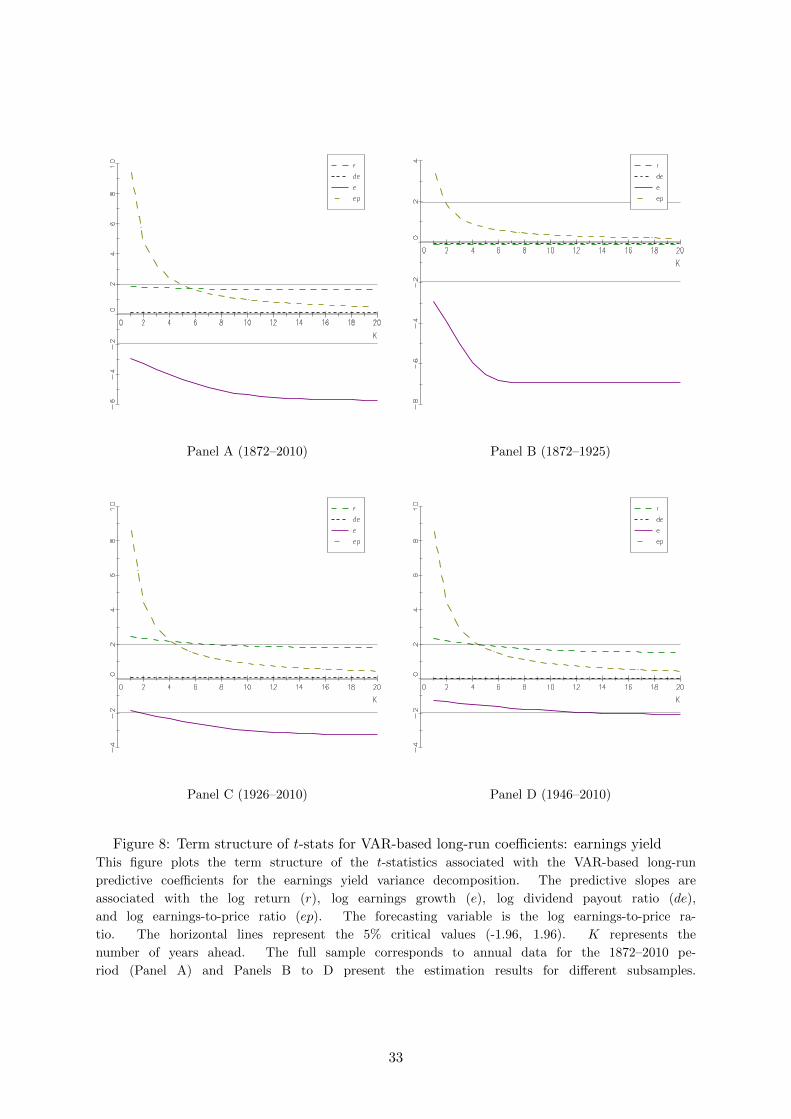
Next, I discuss the VAR-based predictability at several forecasting horizons. The term

structure of predictive coefficients is displayed in Figure 7. In the full sample, the main driver

of variation in e − p is future earnings growth with coefficients around -80% at long horizons

compared to return coefficients around only 20%. The term structure of t-statistics in Figure

8 shows that the earnings growth coefficients are significant at all horizons while there is no

statistical significance (at the 5% level) for the return coefficients. Given the relatively small

persistence of the earnings yield it follows that the slopes associated with future e− p converge

11

relatively fast to zero, achieving values below 10% at the five-year horizon. The respective t-

statistics point to non-significance for K > 5. The long-run implied return and dividend growth

slopes (for K →∞) are 0.21 and -0.79, respectively, which basically correspond to the estimates

associated with K = 20.

By comparing the two subsamples (Panels B and C) we can see that earnings growth pre-

dictability drives almost all the variation of e−p in the first period (slopes around -100%) while

the magnitudes of bKe are somewhat smaller in the modern sample (around -70%). In both

periods the earnings growth coefficients are statistically significant at all horizons. In contrast,

there is no return predictability in the earlier sample (coefficients around zero), while in the

modern sample it turns out that return predictability accounts for around 30% of the variance

of the earnings yield. However, the return slopes are statistically significant (at the 5% level)

only at the near term (K < 8).

In the most recent sample, we observe the highest return predictability in the long-run

(around 40%) while the earnings growth slopes are about -60% at very long horizons. However,

the return slopes are not significant for horizons beyond five years.

4.2 Discussion

By comparing the VAR-based variance decomposition with the benchmark decomposition based

on the long-horizon regressions from the previous section we observe a dramatic change in

the predictability pattern for the modern samples (1926–2010 and 1946–2010). While in the

benchmark case the bulk of variation in e − p is return predictability at long horizons, in

the case of the VAR-based decomposition the main driver of the earnings yield is earnings

growth predictability. Thus, it seems that the first-order VAR misses relevant information

concerning the correlation between the current earnings-to-price ratio and both future returns

and earnings growth at longer horizons, for the modern period. These results also show that

the evidence in Chen, Da, and Priestley (2012) that earnings growth predictability is the main

driver of the earnings yield over this period only holds under the restrictive first-order VAR. In

other words, when one uses the less restrictive long-horizon regressions it follows that return

predictability is the main driver for both the earnings yield and dividend yield, rather than cash

flow predictability, in the modern sample.6

To see better why the (weighted) long-horizon regressions and first-order VAR yield different

6Cochrane (1988) represents another example in which a low-order VAR does not capture long-run dynamics.

12

predictive coefficients at horizons beyond one-year, consider the simplest case of K = 2. In this

case, the return coefficient from the long-horizon regression is given by

β(rt+1 + ρrt+2, et − pt) = β(rt+1, et − pt) + ρβ(rt+2, et − pt)

= br + ρβ(rt+2, et − pt), (17)

where br is the one-year return coefficient, which is the same under the two methodologies. The

implied VAR return coefficient is equal to

br1− ρ2φ2

1− ρφ= br + ρbrφ. (18)

In general, the regression coefficient β(rt+2, et−pt) will be different than brφ, thus explaining the

difference in results from the two methodologies. This difference is likely to be more severe at

longer horizons because the gap above potentially spreads to several periods instead of occurring

only in the second period, as in this simple example. Specifically, in the 1926–2010 sample (for

which there is a greater discrepancy between the VAR-based and direct estimates) the VAR-

based estimates for the return slopes are 0.29, 0.34, and 0.35 at K = 5, K = 10, and K = 20,

respectively, while the corresponding estimates from the long-horizon regressions are 0.41, 0.80,

and 0.93, respectively. The VAR implied earnings growth coefficients are -0.53, -0.63, and -0.65

at K = 5, K = 10, and K = 20, respectively, and the corresponding direct estimates are -0.21,

-0.05, and -0.38, respectively. Thus, the differences in the magnitudes of the estimates between

the two methods tends to increase with horizon, especially, in the case of the return slopes.

Thus, there is a misspecification in the first-order VAR in capturing long-horizon dynamics,

which is magnified at longer horizons.

The punch line of this simple example is that the first-order VAR imposes a restriction on

the true regression coefficients at longer horizons, which might not be confirmed by the data in

some cases. One reason why the results associated with the earnings yield and dividend yield

are qualitatively different in this respect (for the dividend yield the two methodologies yield

relatively similar results while for the earnings yield we have the opposite pattern) is that the

dividend yield is significantly more persistent (higher φ) than the earnings yield in this sample,

as documented in Section 2. Specifically, in the simple example above (K = 2), a high value of

φ may imply that the estimate for β(rt+2, et − pt) will not be significantly different than brφ.

13

5 Monte-Carlo simulation

A part of the return predictability literature has focused on the poor small-sample proper-

ties of long-horizon regressions (see Valkanov (2003), Torous, Valkanov, and Yan (2004), and

Boudoukh, Richardson, and Whitelaw (2008), among others). To address this issue, I conduct

a Monte-Carlo simulation of the VAR model presented in the last section.

I impose a null hypothesis in which there is no return and no earnings growth predictability,

that is, under this null, all the variation of the earnings yield comes from predicting either the

payout ratio or the future earnings yield. Thus, I simulate the first-order VAR by imposing the

restrictions (in the predictive slopes and residuals) associated with this null hypothesis:

rt+1

dt+1 − et+1

∆et+1

et+1 − pt+1

=

0

ρφ−11−ρ

0

φ

(et − pt) +

εrt+1

εdet+1

εrt+1 − (1− ρ)εdet+1 + ρεept+1

εept+1

. (19)

Following Cochrane (2008), in drawing the VAR residuals (10,000 times), I assume that they are

jointly normally distributed and use their covariances from the original sample. The earnings

yield for the base period is simulated as e0 − p0 ∼ N[0,Var(εept+1)/(1− φ2)

]. Armed with the

artificial data, one computes the empirical p-values associated with the return and earnings

growth slopes from the long-horizon regressions, that is, the fractions of simulated estimates for

the return (earnings) coefficients that are higher (lower) than the estimates found in the data.7

The term-structure of empirical p-vales is displayed in Figure 9. We can see that the simu-

lated p-values associated with the return slopes are consistent with the corresponding asymptotic

t-statistics in Figure 6: the return slopes are significant (at the 5% level) in all samples, except

in the 1872–1925 period. In contrast, regarding the earnings growth coefficients it turns out

that the Monte-Carlo and asymptotic inferences lead to some differences in comparison to the

asymptotical inference: in the modern periods (1926–2010 and 1946–2010) the Monte-Carlo

simulation indicates that the earnings coefficients are not significant (with the exception of very

short horizons in the 1926–2010 period), while the Newey-West t-statistics indicate significance

at longer horizons. On the other hand, in the earlier sample the simulated p-values point to

statistical significance of the earnings slopes, although lower than shown by the t-statistics (for

7To make the plots clear, and since the focus of the analysis is on return/earnings predictability, I do notpresent the results for the payout ratio and future earnings yield slopes.

14

horizons between six and 10 years there is only marginal significance, with simulated p-values

around 10%). Moreover, in the full sample, the earnings growth coefficients are significant only

at short or longer horizons based on the simulated p-values, while the asymptotic t-statistics

show significance at all horizons.

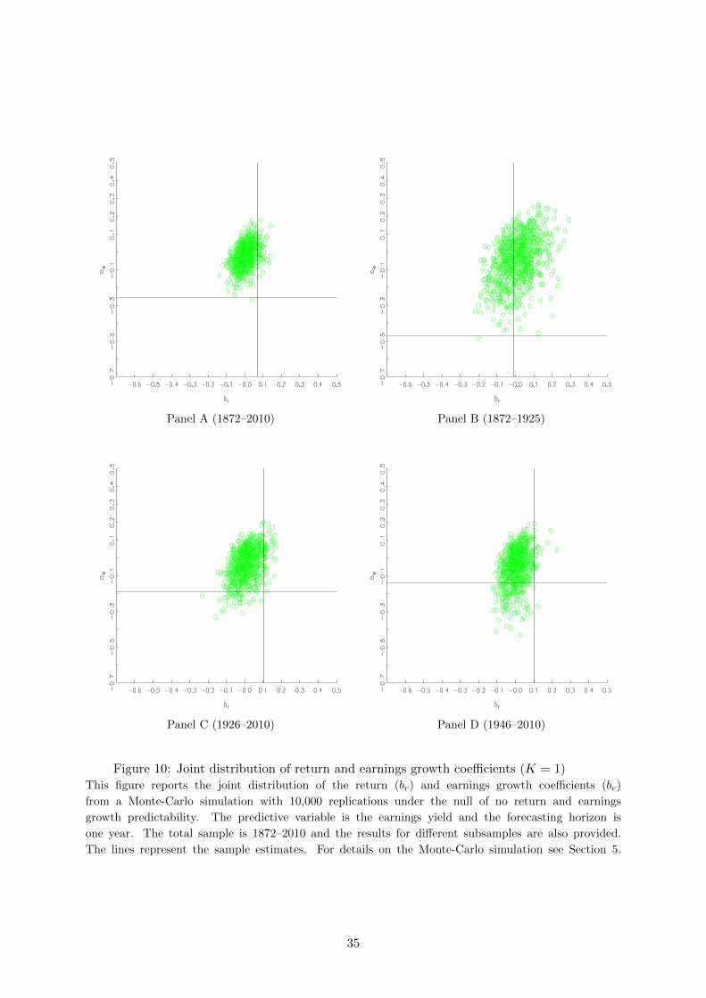
I also present the joint distribution of the return and earnings slopes at the one-year and

20-year horizons in Figures 10 and 11, respectively. To make the plots clear, I only present 1,000

out of the 10,000 pseudo samples. Table 3 presents the fractions of Monte-Carlo replications

under which the return and earnings growth coefficients are higher or lower than the respective

estimates from the original sample.

The results show that at the one-year horizon, in both the full sample and in the earlier

period (1872–1925), we cannot reject (at the 5% level) the joint null of no return or no earnings

growth predictability, with probabilities of 6% (6%+0%) and 56% (56%+0%), respectively. This

is a consequence of not rejecting the null of no return predictability since the null of no earnings

predictability is clearly rejected (probabilities of 0%). In contrast, in the most recent period

(1946–2010) the joint null is not rejected with a probability of 18% (16%+2%) because the null

of no earnings predictability is not rejected (probability of 16%).

When we consider a long forecasting horizon (20 years), we have a different picture in the

full sample: the joint null is again not rejected (11%) mainly due to the non-rejection of the null

of no earnings predictability (probability of 9%). On the other hand, the results for the earlier

period are qualitatively similar to those obtained for the one-period slopes. In the modern

periods (1926–2010 and 1946–2010), the non-rejection of the joint null arises because we cannot

reject the null of no cash flow predictability (probabilities of 49% and 64%, respectively).

Overall, this Monte carlo simulation confirms the findings from Section 3: the predictability

of earnings growth drives the earnings yield in the earlier sample, while return predictability

represents the bulk of variation of the earnings-to-price ratio in the modern period.

6 Does the earnings yield forecasts the equity premium?

In this section, I analyze the predictability of the earnings yield for future excess stock returns

rather than nominal returns. The goal is to check whether the main results obtained in Section 3

for the case of returns, also hold for excess returns, which has been the focus of the predictability

literature (see, for example, Campbell and Thompson (2008), Goyal and Welch (2008), and Maio

15

(2012b), among others).

By adding and subtracting the one-period interest rate, rf,t+j , it is straightforward to derive

the following present-value relation of the earnings yield in terms of future equity premia, ret+j :

et − pt =−c(1− ρK)

1− ρ+

K∑j=1

ρj−1ret+j − (1− ρ)

K∑j=1

ρj−1(dt+j − et+j)−K∑j=1

ρj−1∆et+j

+K∑j=1

ρj−1rf,t+j + ρK(et+K − pt+K), (20)

which states that conditional on the other variables, the current earnings yield is positively

correlated with both future excess returns and short-term interest rates.

To analyze the earnings yield predictability for excess stock returns, I conduct the following

weighted long-horizon regressions:

K∑j=1

ρj−1ret+j = aKr + bKr (et − pt) + εrt+K , (21)

K∑j=1

ρj−1∆et+j = aKe + bKe (et − pt) + εet+K , (22)

(1− ρ)

K∑j=1

ρj−1(dt+j − et+j) = aKde + bKde(et − pt) + εdet+K , (23)

K∑j=1

ρj−1rf,t+j = aKf + bKf (et − pt) + εft+K , (24)

ρK(et+K − pt+K) = aKep + bKep(et − pt) + εept+K , (25)

where the differences relative to the set of regressions conducted in Section 3 are the inclusion of

a regression for future interest rates, and the fact that one now forecasts excess returns rather

than returns. By combing these predictive regressions with the dynamic present-value relation

in (20) one obtains the following variance decomposition for the earnings yield:

1 = bKr − bKde − bKe + bKf + bKep. (26)

Essentially, this new variance decomposition is similar to the one presented in (15), and de-

composes the return slope into an excess return coefficient, bKr , and an interest rate effect, bKf .

The proxy for the one-period interest rate is the annual Treasury-bill rate, available from Amit

Goyal’s webpage.

16

The term structure of slope estimates, and respective t-statistics, are presented in Figures 12

and 13, respectively. In the full sample the interest rate coefficients are quite small in magnitude

and non-significant at all horizons. This implies that the equity premium slopes are very similar

to the return coefficients in Figure 5. Moreover, similarly to the return slopes, the estimates for

the excess return coefficients are significant at most horizons.

In the earlier period, the interest rate coefficients achieve values around 10% at very long

horizons, and these estimates are significant at all horizons. This implies that the equity pre-

mium slopes go more in the wrong direction (negative values) than the corresponding return

slopes, at longer horizons (these coefficients are significant for horizons greater than 16 years).

In the modern sample, the estimates for bKf reach their maximum (around 10%) for horizons

between 8 and 12 years. However, there is no statistical significance for the interest rate slopes

at any horizon. At long horizons, the equity premium coefficients are very close to the corre-

sponding return estimates, and are also statistically significant.

For the most recent sample (1946–2010), the interest rate coefficients become negative for

horizons greater than 16 years (close to -20% at K = 20), although they are not significant. This

implies that the amount of excess return predictability is even stronger than the corresponding

return predictability, with estimates above 130% at the longer horizons. These estimates are

strongly significant, especially for large K.

Therefore, these results show that using a variance decomposition based on excess returns

does not change the main result from Section 3: in the earlier period, the bulk of variation in

the earnings yield is earnings growth predictability while in the second period it is all about

predictability in market discount rates.

7 Conclusion


and earnings growth by imposing the restrictions associated with a present-value relation. I

define a term structure of variance decompositions for the earnings-to-price ratio: at each

forecasting horizon (from one to 20 years ahead) the variation in the earnings yield is the result

of four types of predictability from this financial ratio: predictability of future returns, earnings

growth predictability, predictability of future payout ratios, or the predictability of the earnings

yield at some future date.

17

By estimating weighted long-horizon regressions for the 1872–1925 and 1926–2010 periods

I find a reversal in return/earnings growth predictability from the earnings yield: in the earlier

period, the bulk of variation in the earnings yield is predictability of earnings growth, while

in the modern sample what drives the earnings-to-price ratio is return predictability. These

results are consistent with the findings in Cochrane (2008, 2011) and Chen (2009), based on

a VAR-based variance decomposition for the market dividend yield, which show that most

of the variation in the dividend yield in the earlier period is attributable to dividend growth

predictability, while in the later period the main driver is return predictability.

Furthermore, the finding in this paper is opposite to the result in Chen, Da, and Priest-

ley (2012) that the key driver of the market earnings yield in the modern period is earnings

growth, rather than return, predictability. I show that their results only hold when the variance

decomposition for the earnings yield is based on a first-order VAR. Thus, this paper makes a

contribution to the debate on using long-horizon regressions to estimate predictive coefficients

at long horizons versus the alternative approach of obtaining implied estimates from a short-

order VAR, which has been widely used in the related literature. I show that, in the 1926–2010

period, the two approaches yield similar results when the predicting variable is the dividend

yield, but quite opposing results when the forecasting variable is the earnings yield. In other

words, the restrictions imposed by the first-order VAR are not validated by the data when the

predictor is the earnings yield.

Therefore, the results in this paper are inconsistent with a dividend smoothing argument

behind the changing predictability pattern of dividend yield over the two periods, as argued by

Chen, Da, and Priestley (2012). Instead, I argue that this reversal in predictability associated

with both the earnings and dividend yield is a consequence of the changing characteristics and

risk-return profiles of the average firm in the U.S. stock market over time.

I conduct a Monte-Carlo simulation by imposing the null of no return and no earnings

growth predictability, that is, under this null all the variation of the earnings yield comes from

predicting the payout ratio or the future earnings yield. The Monte-Carlo p-values confirm the

asymptotic t-statistics associated with the predictive slopes from the long-horizon regressions:

in the earlier period, one rejects the null of no earnings growth predictability, while one cannot

reject the null of no return predictability. In the modern sample, we have exactly opposite

results.

I derive and estimate a variance decomposition for the earnings yield in terms of excess

18

returns rather than returns. The results are qualitatively similar to the benchmark variance

decomposition based on returns since the market earnings yield has little forecasting power for

future interest rates.

19

References

Binsbergen, J., and R. Koijen, 2010, Predictive regressions: A present-value approach, Journal

of Finance 65, 1439–1471.

Boudoukh, J., M. Richardson, and R. Whitelaw, 2008, The myth of long-horizon predictability,

Review of Financial Studies 21, 1577–1605.

Brav, A., J. Graham, C. Harvey, and R. Michaely, 2005, Payout policy in the 21st century,

Journal of Financial Economics 77, 483–527.

Campbell, J., and R. Shiller, 1988a, The dividend price ratio and expectations of future divi-

dends and discount factors, Review of Financial Studies 1, 195–228.

Campbell, J., and R. Shiller, 1988b, Stock prices, earnings, and expected dividends, Journal of

Finance 43, 661–676.

Campbell, J., and R. Shiller, 1998, Valuation ratios and the long-run stock market outlook,

Journal of Portfolio Management 24, 11–26.

Campbell, J., and S. Thompson, 2008, Predicting excess stock returns out of sample: Can

anything beat the historical average? Review of Financial Studies 21, 1509–1531.

Campbell, J., and T. Vuolteenaho, 2004, Bad beta, good beta, American Economic Review 94,

1249–1275.

Campbell, J., and M. Yogo, 2006, Efficient tests of stock return predictability, Journal of Fi-

nancial Economics 81, 27–60.

Chen, L., 2009, On the reversal of return and dividend growth predictability: A tale of two

periods, Journal of Financial Economics 92, 128–151.

Chen, L., Z. Da, and R. Priestley, 2012, Dividend smoothing and predictability, Management

Science 58, 1834–1853.

Cochrane, J., 1988, How big is the random walk in GNP? Journal of Political Economy 96,

893–920.

Cochrane, J., 1992, Explaining the variance of price-dividend ratios, Review of Financial Studies

5, 243–280.

Cochrane, J., 2008, The dog that did not bark: A defense of return predictability, Review of

Financial Studies 21, 1533–1575.

20

Cochrane, J., 2011, Presidential address: Discount rates, Journal of Finance 66, 1047–1108.

Cohen, R., C. Polk, and T. Vuolteenaho, 2003, The value spread, Journal of Finance 58, 609–

641.

Cornell, B., 1999, Risk, duration, and capital budgeting: New evidence on some old questions,

Journal of Business 72, 183–200.

D’Avolio, G., 2002, The market for borrowing stock, Journal of Financial Economics 66, 271–

306.

Engsted, T., and T. Pedersen, 2010, The dividend-price ratio does predict dividend growth:

International evidence, Journal of Empirical Finance 17, 585–605.

Fama, E., and K. French, 2001, Disappearing dividends: changing firm characteristics or lower

propensity to pay? Journal of Financial Economics 60, 3–43.

Goyal, A., and I. Welch, 2008, A comprehensive look at the empirical performance of equity

premium prediction, Review of Financial Studies 21, 1455–1508.

Kelly, B., and S. Pruitt, 2012, Market expectations in the cross section of present values,

Working paper, Chigago Booth School of Business.

Koijen, R., and S. Van Nieuwerburgh, 2011, Predictability of returns and cash flows, Annual

Review of Financial Economics 3, 467–491.

Lacerda, F., and P. Santa-Clara, 2010, Forecasting dividend growth to better predict returns,

Working paper, Nova School of Business and Economics.

Lamont, O., 1998, Earnings and expected returns, Journal of Finance 53, 1563–1587.

Larrain, B., and M. Yogo, 2008, Does firm value move too much to be justified by subsequent

changes in cash flow? Journal of Financial Economics 87, 200–226.

Leary, M., and R. Michaely, 2011, Determinants of dividend smmothing: Empirical evidence,


Lettau, M., and S. Van Nieuwerburgh, 2008, Reconciling the return predictability evidence,


Maio, P., 2012a, Intertemporal CAPM with conditioning variables, Management Science, forth-

coming.

21

Maio, P., 2012b, The ‘Fed model’ and the predictability of stock returns, Review of Finance,

forthcoming.

Maio, P., and P. Santa-Clara, 2012a, Dividend yields, dividend growth, and return predictability

in the cross-section of stocks, Working paper, Hanken School of Economics.

Maio, P., and P. Santa-Clara, 2012b, Multifactor models and their consistency with the ICAPM,

Journal of Financial Economics, forthcoming.

Mitchell, M., T. Pulvino, and E. Stafford, 2002, Limited arbitrage in equity markets, Journal

of Finance 57, 551–584.

Newey, W., and K. West, 1987, A simple, positive semi-definite, heteroskedasticity and auto-

correlation consistent covariance matrix, Econometrica 55, 703–708.

Polk, C., S. Thompson, and T. Vuolteenaho, 2006, Cross-sectional forecasts of the equity pre-

mium, Journal of Financial Economics 81, 101–141.

Rangvid, J., M. Schmeling, and A. Schrimpf, 2011, Dividend predictability around the world,

Working paper, Copenhagen Business School.

Sadka, G., 2007, Understanding stock price volatility: The role of earnings, Journal of Account-

ing Research 45, 199–228.

Torous, W., R. Valkanov, and S. Yan, 2004, On predicting stock returns with nearly integrated

explanatory variables, Journal of Business 77, 937–966.

Valkanov, R., 2003, Long-horizon regressions: Theoretical results and applications, Journal of

Financial Economics 68, 201–232.

22

A Delta method for standard errors of VAR-based coefficients

To compute the asymptotic standard errors of the VAR-based predictive coefficients, bK ≡(bKr , b

Kde, b

Ke , b

Kep

)′, I use the delta method:

Var(bK) =∂bK

∂b′Var(b)

∂bK

∂b, (A.1)

where b ≡ (br, bde, be, φ)′ denotes the vector of VAR slopes. The matrix of derivatives is givenby:

∂bK

∂b′≡

∂bKr∂br

∂bKr∂bde

∂bKr∂be

∂bKr∂φ

∂bKde∂br

∂bKde∂bde

∂bKde∂be

∂bKde∂φ

∂bKe∂br

∂bKe∂bde

∂bKe∂be

∂bKe∂φ

∂bKep∂br

∂bKep∂bde

∂bKep∂be

∂bKep∂φ

=

1−ρKφK1−ρφ 0 0 −KbrρKφK−1(1−ρφ)+ρbr(1−ρKφK)

(1−ρφ)2

0 (1− ρ)1−ρKφK

1−ρφ 0 −KbdeρKφK−1(1−ρφ)(1−ρ)+ρbde(1−ρKφK)(1−ρ)(1−ρφ)2

0 0 1−ρKφK1−ρφ

−KbeρKφK−1(1−ρφ)+ρbe(1−ρKφK)(1−ρφ)2

0 0 0 KρKφK−1

. (A.2)

23

Table 1: Descriptive statisticsThis table reports descriptive statistics for the log market return (r); log dividend-to-price ra-

tio (d − p); log earnings-to-price ratio (e − p); log dividend payout ratio (d − e); log divi-

dend growth (∆d); and log earnings growth (∆e). The sample is 1872–2010. φ designates

the first-order autocorrelation. The correlations between the variables are presented in Panel B.

Panel AMean Stdev. Min. Max. φ

r 0.084 0.179 -0.540 0.425 0.022d− p -3.190 0.427 -4.478 -2.288 0.879e− p -2.664 0.380 -4.106 -1.670 0.706d− e -0.526 0.313 -1.225 0.646 0.591∆d 0.032 0.124 -0.495 0.427 0.252∆e 0.038 0.297 -1.492 1.231 -0.069

Panel Br d− p e− p d− e ∆d ∆e

r 1.00 -0.30 -0.08 -0.31 0.05 0.34d− p 1.00 0.70 0.51 -0.07 -0.19e− p 1.00 -0.25 0.24 0.29d− e 1.00 -0.38 -0.61∆d 1.00 0.31∆e 1.00

24

Table 2: VAR estimatesThis table reports the one-year restricted VAR estimation results when the predictor is the market earn-

ings yield. The variables in the VAR are the log stock return (r), log earnings growth (∆e), log dividend

payout ratio (d− e), and log earnings-to-price ratio (e− p). b(φ) denote the VAR slopes associated with

lagged e−p, while t denotes the respective Newey and West (1987) t-statistics (calculated with one lag).

bi(φi) denote the slope estimates implied from the variance decomposition for e − p, and t denote the

respective asymptotic t-statistics computed under the Delta method. R2(%) is the coefficient of determi-

nation for each equation in the VAR, in %. The full sample corresponds to annual data for the 1872–2010

period (Panel A) and Panels B to D present the estimation results for different subsamples. Italic, un-

derlined, and bold numbers denote statistical significance at the 10%, 5%, and 1% levels, respectively.

b(φ) t bi(φi) t R2(%)Panel A (1872-2010)

r 0.068 1 .82 0.071 1 .88 2.10d− e 0.050 0.61 −0.022 −0.31 0.37∆e −0.253 −2.93 −0.256 −2.98 10.51e− p 0.706 9.65 0.709 9.66 49.85

Panel B (1872-1925)r −0.007 −0.10 −0.009 −0.14 0.02

d− e −0.084 −0.69 −0.031 −0.27 0.91∆e −0.469 −2.92 −0.467 −2.90 22.16e− p 0.563 3.56 0.561 3.56 31.29

Panel C (1926-2010)r 0.101 2.44 0.103 2.48 4.74

d− e 0.029 0.35 −0.021 −0.30 0.15∆e −0.189 −1 .86 −0.190 −1 .88 6.85e− p 0.735 8.85 0.737 8.85 54.42

Panel D (1946-2010)r 0.100 2.32 0.100 2.31 7.69

d− e 0.012 0.17 0.025 0.34 0.04∆e −0.141 −1.27 −0.141 −1.26 4.30e− p 0.783 8.76 0.783 8.76 61.32

Table 3: Probability values for return and earnings growth slopesThis table reports the fractions of Monte-Carlo simulated values of the return (bKr ) and earnings

growth coefficients (bKe ) that are higher/lower than the respective estimates from the original sam-

ple (bKr,0, bKe,0). The predictive variable is the earnings yield and the forecasting horizon is one

year (Panel A) and 20 years ahead (Panel B). The total sample is 1872–2010 and the results for

different subsamples are also provided. For details on the Monte-Carlo simulation see Section 5.

(bKr < bKr,0, bKe > bKe,0) (bKr > bKr,0, b

Ke > bKe,0) (bKr < bKr,0, b

Ke < bKe,0) (bKr > bKr,0, b

Ke < bKe,0)

Panel A (K = 1)1872–2010 0.94 0.06 0.00 0.001872–1925 0.44 0.56 0.00 0.001926–2010 0.91 0.05 0.04 0.001946–2010 0.82 0.02 0.16 0.00

Panel B (K = 20)1872–2010 0.89 0.02 0.09 0.001872–1925 0.13 0.86 0.01 0.001926–2010 0.50 0.01 0.49 0.001946–2010 0.36 0.00 0.64 0.00

25

Figure 1: Dividend yield and Earnings yieldThis figure plots the time-series for the market dividend-to-price (d/p) and

earnings-to-price (e/p) ratios (original series). The sample is 1872–2010.

26

Panel A (∆d,∆e)

Panel B (d/e)

Figure 2: Dividend growth, earnings growth, and dividend payout ratioThis figure plots the time-series for the aggregate dividend (∆d) and earnings growth rates

(∆e) (Panel A), and the dividend payout ratio (Panel B). The sample is 1872–2010.

27

Panel A (1872–2010) Panel B (1872–1925)

Panel C (1926–2010) Panel D (1946–2010)

Figure 3: Term structure of direct long-run coefficients: dividend yieldThis figure plots the term structure of direct long-run predictive coefficients for the variance

decomposition associated with the dividend yield. The predictive slopes are associated with

the log return (r), log dividend growth (d), and log dividend-to-price ratio (dp). The fore-

casting variable is the log dividend-to-price ratio. “sum” denotes the value of the variance

decomposition, in %. The long-run coefficients are measured in %, and K represents the

number of years ahead. The full sample corresponds to annual data for the 1872–2010 pe-

riod (Panel A) and Panels B to D present the estimation results for different subsamples.

28

Panel A (1872–2010) Panel B (1872–1925)

Panel C (1926–2010) Panel D (1946–2010)

Figure 4: Term structure of t-stats for direct long-run coefficients: dividend yieldThis figure plots the term structure of the t-statistics associated with the direct long-run predictive

coefficients for the dividend yield variance decomposition. The predictive slopes are associated with

the log return (r), log dividend growth (d), and log dividend-to-price ratio (dp). The forecasting vari-

able is the log dividend-to-price ratio. The horizontal lines represent the 5% critical values (-1.96,

1.96). K represents the number of years ahead. The full sample corresponds to annual data for the

1872–2010 period (Panel A) and Panels B to D present the estimation results for different subsamples.

29

Panel A (1872–2010) Panel B (1872–1925)

Panel C (1926–2010) Panel D (1946–2010)

Figure 5: Term structure of direct long-run coefficients: earnings yieldThis figure plots the term structure of direct long-run predictive coefficients for the variance de-

composition associated with the earnings yield. The predictive slopes are associated with the log

return (r), log earnings growth (e), log dividend payout ratio (de), and log earnings-to-price ra-

tio (ep). The forecasting variable is the log earnings-to-price ratio. “sum” denotes the value

of the variance decomposition, in %. The long-run coefficients are measured in %, and K rep-

resents the number of years ahead. The full sample corresponds to annual data for the 1872–

2010 period (Panel A) and Panels B to D present the estimation results for different subsamples.

30

Panel A (1872–2010) Panel B (1872–1925)

Panel C (1926–2010) Panel D (1946–2010)

Figure 6: Term structure of t-stats for direct long-run coefficients: earnings yieldThis figure plots the term structure of the t-statistics associated with the direct long-run predictive coeffi-

cients for the earnings yield variance decomposition. The predictive slopes are associated with the log re-

turn (r), log earnings growth (e), log dividend payout ratio (de), and log earnings-to-price ratio (ep). The

forecasting variable is the log earnings-to-price ratio. The horizontal lines represent the 5% critical values

(-1.96, 1.96). K represents the number of years ahead. The full sample corresponds to annual data for the


31

Panel A (1872–2010) Panel B (1872–1925)

Panel C (1926–2010) Panel D (1946–2010)

Figure 7: Term structure of VAR-based long-run coefficients: earnings yieldThis figure plots the term structure of the VAR-based long-run predictive coefficients for the vari-

ance decomposition associated with the earnings yield. The predictive slopes are associated with

the log return (r), log earnings growth (e), log dividend payout ratio (de), and log earnings-to-

price ratio (ep). The forecasting variable is the log earnings-to-price ratio. “sum” denotes the

value of the variance decomposition, in %. The long-run coefficients are measured in %, and K

represents the number of years ahead. The full sample corresponds to annual data for the 1872–


32

Panel A (1872–2010) Panel B (1872–1925)

Panel C (1926–2010) Panel D (1946–2010)

Figure 8: Term structure of t-stats for VAR-based long-run coefficients: earnings yieldThis figure plots the term structure of the t-statistics associated with the VAR-based long-run

predictive coefficients for the earnings yield variance decomposition. The predictive slopes are

associated with the log return (r), log earnings growth (e), log dividend payout ratio (de),

and log earnings-to-price ratio (ep). The forecasting variable is the log earnings-to-price ra-

tio. The horizontal lines represent the 5% critical values (-1.96, 1.96). K represents the

number of years ahead. The full sample corresponds to annual data for the 1872–2010 pe-

riod (Panel A) and Panels B to D present the estimation results for different subsamples.

33

Panel A (1872–2010) Panel B (1872–1925)

Panel C (1926–2010) Panel D (1946–2010)

Figure 9: Term-structure of simulated p-valuesThis figure plots the simulated p-values for the return (r) and earnings growth (e) slopes from a Monte-

Carlo simulation with 10,000 replications under the null of no return and earnings growth predictability.

The predictive variable is the earnings yield. The numbers indicate the fraction of pseudo samples under

which the return (earnings growth) coefficient is higher (lower) than the corresponding estimates from the

original sample. K represents the number of years ahead. The total sample is 1872–2010 and the results

for different subsamples are also provided. For details on the Monte-Carlo simulation see Section 5.

34

Panel A (1872–2010) Panel B (1872–1925)

Panel C (1926–2010) Panel D (1946–2010)

Figure 10: Joint distribution of return and earnings growth coefficients (K = 1)This figure reports the joint distribution of the return (br) and earnings growth coefficients (be)

from a Monte-Carlo simulation with 10,000 replications under the null of no return and earnings

growth predictability. The predictive variable is the earnings yield and the forecasting horizon is

one year. The total sample is 1872–2010 and the results for different subsamples are also provided.

The lines represent the sample estimates. For details on the Monte-Carlo simulation see Section 5.

35

Panel A (1872–2010) Panel B (1872–1925)

Panel C (1926–2010) Panel D (1946–2010)

Figure 11: Joint distribution of return and earnings growth coefficients (K = 20)This figure reports the joint distribution of the return (br) and earnings growth coefficients (be)

from a Monte-Carlo simulation with 10,000 replications under the null of no return and earnings

growth predictability. The predictive variable is the earnings yield and the forecasting horizon is

20 years. The total sample is 1872–2010 and the results for different subsamples are also provided.

The lines represent the sample estimates. For details on the Monte-Carlo simulation see Section 5.

36

Panel A (1872–2010) Panel B (1872–1925)

Panel C (1926–2010) Panel D (1946–2010)

Figure 12: Term structure of direct long-run coefficients: excess returnsThis figure plots the term structure of direct long-run predictive coefficients for the variance decom-

position associated with the earnings yield. The predictive slopes are associated with the excess log

return (r), log earnings growth (e), log dividend payout ratio (de), log short-term interest rate (f),

and log earnings-to-price ratio (ep). The forecasting variable is the log earnings-to-price ratio. “sum”

denotes the value of the variance decomposition, in %. The long-run coefficients are measured in %,

and K represents the number of years ahead. The full sample corresponds to annual data for the


37

Panel A (1872–2010) Panel B (1872–1925)

Panel C (1926–2010) Panel D (1946–2010)

Figure 13: Term structure of t-stats for direct long-run coefficients: excess returnsThis figure plots the term structure of the t-statistics associated with the direct long-run predic-

tive coefficients for the earnings yield variance decomposition. The predictive slopes are associ-

ated with the excess log return (r), log earnings growth (e), log dividend payout ratio (de), log

short-term interest rate (f), and log earnings-to-price ratio (ep). The forecasting variable is the

log earnings-to-price ratio. The horizontal lines represent the 5% critical values (-1.96, 1.96). K

represents the number of years ahead. The full sample corresponds to annual data for the 1872–


38

the long-run relation between returns, earnings, and dividends · the long-run relation between...

Documents