THE MULTI-INDEX MODEL AND

PRACTICAL PORTFOLIO ANALYSIS

James L. Farrell, Jr., C.F.A.

Occasional Paper Number 4

THEFINANCIALANALYSTSRESEARCHFOUNDATION

Copyright © 1976

by The Financial Analysts Research FoundationCharlottesville, Virginia

10-digit ISBN: 1-934667-06-4 13-digit ISBN: 978-1-93466706-4

CONTENTS

Dedication VI

Foreword VII

Acknowledgment IX

I. Introduction 1

II. Portfolio Selection Models 3Markowitz Model 3Single-Index Model 7Multi-Index Model 9

III. Empirical Test and Multi-Index Model Inputs 11

Empirical Evaluation of Portfolio Selection Models 11

Market and Industry Factors 13Potential Additional Factor 15

IV. Empirical Test of Stock Grouping Hypothesis 18

Selection of Test Sample 18

Statistical Analysis of Sample 21

Cluster Analysis 23Index Procedure 24Significance of Group Effects 28

V. Test of Relative Performance of Multi-Index Model 30Analysis of Index Model Specifications 30Ex-Ante Correlation Matrices 32Ex-Ante Efficient Portfolios 33Ex-Post Performance . 36Test of Stability of Input Relationships 44

VI Summary and Conclusion 47

iii

THE FINANCIAL ANALYSTS RESEARCH FOUNDATIONAND ITS PUBLICATIONS

1. The Financial Analysts Research Foundation is an autonomous charitablefoundation, as defined by Section 501(c)(3) of the Internal Revenue Code.The Foundation seeks to improve the professional performance of financialanalysts by fostering education, by stimulating the development of financialanalysis through high quality research, and by facilitating the dissemination ofsuch research to users and to the public. More specifically, the purposes andobligations of the Foundation are to commission basic studies (1) with respectto investment securities analysis, investment management, financial analysis,securities markets and closely related areas that are not presently oradequately covered by the available literature, (2) that are directed toward thepractical needs of the financial analyst and the portfolio manager, and (3) thatare of some enduring value. Within the constraints of the above obligations,the Foundation cooperates with other organizations, such as The FinancialAnalysts Federation and The Institute of Chartered' Financial Analysts, that toa substantial degree share mutual interests and objectives.

2. Several types of studies and publications are authorized:

A. Studies based on existing knowledge or methodology which result in adifferent arrangement of the subject. Included in this category are papersthat seek to broaden the understanding within the profession of financialanalysis through reviewing, distilling, or synthesizing previously publishedtheoretical research, empirical findings, and specialized literature;

B. Studies that apply known techniques, methodology, and quantitativemethods to problems of financial analysis;

C. Studies that develop new approaches or new solutions to importantproblems existing in financial analysis;

D. Pioneering and original research that discloses new theories, newrelationships, or new knowledge that confirms, rejects, or extendsexisting theories and concepts in financial analysis. Ordinarily, suchresearch is intended to improve the state of the art. The research findingsmay be supported by the collection or manipulation of empirical ordescriptive data from primary sources, such as original records, fieldinterviews, or surveys.

3. The views expressed in the publications are those of the authors and do notnecessarily represent the official position of the Foundation, its Board ofTrustees, or its staff. As a matter of policy, the Foundation has no officialposition with respect to specific practices in financial analysis.

4. The Foundation is indebted to the voluntary financial support of itsinstitutional and individual sponsors by which this and other publications aremade possible. As a 501(c)(3) foundation, contributions are welcomed frominterested donors, including individuals, business organizations, institutions,estates, foundations, and others. Inquiries may be directed to:

Executive DirectorThe Financial Analysts Research FoundationUniversity of Virginia, Post Office Box 3668Charlottesville, Virginia 22903

(804) 977-6600

IV

THE FINANCIAL ANALYSTS RESEARCH FOUNDATION

1975-1976

Board of Trustees and Officers

Jerome L. Valentine, C.F.A., PresidentFinancial Consultant, Houston

Robert D. Milne, C.F.A., Vice PresidentBoyd, Watterson & Co., Cleveland

Leonard E. Barlow, C.F.A., SecretaryMcLeod, Young, Weir & Company LimitedTorontoW. Scott Bauman, C.F .A., Executive Director

and TreasurerUniversity of Virginia, Charlottesville

Frank E. Block, C.F.A.Shields Model Roland IncorporatedNew York

M. Harvey Earp, C.F.A.Brittany Capital Corporation, Dallas

Roger F. MurrayColumbia University, New York

Jack L. TreynorFinancial Analysts JournalNew York

Ex-Off£cio

Walter S. McConnell, C.F .A.Wertheim & Co., Inc., New YorkChairman, The Financial Analysts Federation

Walter P. Stern, C.F.A.Capital Research Company, New YorkPresident, The Institute of Chartered

Financial AnalystsC. Stewart SheppardUniversity of VirginiaDean, The Colgate Darden Graduate School

of Business Administration

Finance Committee

C. Stewart Sheppard, ChairmanUniversity of Virginia, Charlottesville

Gordon R. Ball, C.F.A.Martens, Ball, Albrecht Securities LimitedTorontoLeonard E. Barlow, C.F.A.McLeod, Young, Weir & Company LimitedToronto

George S. Bissell, C.F .A.Massachusetts Financial Services, Inc.Boston

Calvin S. Cudney, C.F .A.The Cleveland Trust CompanyCleveland

William R. Grant, C.F .A.Smith Barney, Harris Upham & Co. IncorporatedNew York

William S. Gray, III, C.F .A.Harris Trust and Savings Bank, Chicago

Robert E. Gunn, C.F.A.Financial Counselors, Inc., Kansas CityFrank X. Keaney, C.F .A.Stifel, Nicolaus & Company IncorporatedSt. Louis

George Stevenson Kemp, Jr., C.F .A.Paine, Webber, Jackson & Curtis Inc.Richmond

W. Scott Bauman, C.F .A., Executive Directorand Treasurer

University of VirginiaCharlottesville

Richard W. Lambourne, C.F.A.Crocker Investment Management CorporationSan Francisco

James G. McCormick, C.F.A.Eppler, Guerin & Turner, Inc.Dallas

David G. Pearson, C.F.A.Blyth Eastman Dillon & Co. IncorporatedLos Angeles

LeRoy F. Piche, C.F.A.Northwest Bancorporation, Minneapolis

Morton Smith, C.F .A.Philadelphia

Raymond L. Steele, C.F.A.The Robinson-Humphrey Company, Inc.Atlanta

David G. Watterson, C.F.A.Boyd, Watterson & Co., Cleveland

David D. Williams, C.F .A.National Bank of DetroitDetroit

Gordon T. Wise, C.F.A.First National Advisors, Inc.Houston

Staff

Hartman L. Butler,Jr., C.F.A.Research Administrator

The Financial Analysts Research FoundationCharlottesville

v

This publication was financed in part by a grant from TheInstitute of Chartered Financial Analysts made under the C. StewartSheppard Award, iln award that was presented to Dr. C. StewartSheppard in recognition of his outstanding contribution, throughdedicated effort and inspiring leadership, in advancing The Institute ofChartered Financial Analysts as a vital force in fostering the educationof financial analysts, establishing high ethical standards of conduct, anddeveloping programs and publications to encourage the continuingeducation of financial analysts.

vi

FOREWORD

This publication represents the fourth in the Occasional PaperSeries, 'i series that is intended to cover a variety of topics of interest tofinancial analysts, presented in a length that is longer than a journalarticle but shorter than a full length book.

Major new approaches and techniques to investment managementhave been introduced in recent years to assist portfolio managers inestimating returns and in controlling risk levels in their portfolios. Thelinear single-index model that uses a beta coefficient has receivedconsiderable attention and discussion among professional analysts. Theauthor of this paper reviews three major portfolio models and presentsa multi-index model that has a potential of being a significantly usefulextension to the existing single-index model and to beta theory.

We are extremely grateful to the author, Dr. James L. Farrell,Jr.,C.F .A., for his outstanding piece ofresearch and his well written paper.

We wish to express our appreciation to those who served on thisProject Committee, Mr. Jack L. Treynor, Dr. Jerome L. Valentine,C.F.A., and Dr. Roger F. Murray, and to Hartman L. ButIer,Jr., C.F.A.,for editorial review and coordination of the project.

w. Scott Bauman, G.F.A.Executive Director

VII

ACKNOWLEDGMENT

There were numerous persons who contributed to this study. I amgrateful to Roger Murray who provided much inspiration when atCREF and a great deal of encouragement since then in developing manyof the concepts of portfolio management discussed in the paper. MartinGruber contributed substantially in the initial stages of the project andoffered helpful suggestions at various other times. I appreciate theopportunity provided by Robert Ferguson of the Institute forQuantitative Research in Finance to refine some ideas at a recentseminar. Scott Bauman and others of The Financial Analysts ResearchFoundation were most helpful at all stages in the process ofpublication. Finally, my wife Cyrille's typing, editing and generalencouragement greatly facilitated completion of this study.

July, 1976

IX

IL.F.

I. Introduction

Modern portfolio analysis is concerned with grouping individualinvestments into an efficient set of portfolios. A portfolio is definedas efficient if (and only if) it offers a higher overall expected returnthan any other portfolio with comparable risk. Three analyticalmethods for developing efficient sets of portfolios are: (1) Markowitzmodel; 1 (2) Sharpe single-index model;2 and (3) Cohen and Pogue'smulti-index model.3

The Markowitz model established the basic framework formodern portfolio analysis and provides the most accurately developedset of efficient portfolios. The size and complexity of the model,however, makes it virtually inapplicable for practical use. The Sharpemodel economizes on inputs and computer time but neglects importantrelationships among securities. Failure to assess these relationshipsresults in a set of portfolios that is less than truly efficient. Cohen andPogue's multi-index model provides a means of accounting for theserelationships while at the same time achieving substantial input andcomputational savings over the Markowitz technique. The multi-indexmodel should thus be the preferred technique for practical portfolioanalysis.

The essential problem in using the multi-index model isdeveloping appropriate inputs. Industry groups have been tested in themodel but do not provide inputs that allow it to operate at maximumefficiency. Needed are indexes of stock returns that are homogeneousin the sense of being significantly correlated within their own groupingand, at the same time, generally independent of other groups.

1. HalTY M. Markowitz, Portfolio Selection: Efficient Diversification ofInvestments, (New York: John Wiley & Sons, Inc.), 1959.

2. William F. Sharpe, "A Simplified Model for Portfolio Selection,"Management Science, January 1963, pp. 277-293.

3. Kalman J. Cohen and Jerry A. Pogue, "An Empirical Evaluation ofAlternative Portfolio Selection Models," ] oumal of Business, April 1967, pp.166-193.

1

The writer has shown that it is in fact possible to develop stockgroupings with such desirable collinearity characteristics.4 A studywas undertaken to use indexes constructed from these stock groupingsas inputs to the multi-index model, and to test that model's perfor­mance against the performance of the Sharpe and Markowitz models.

This study proceeds as follows. Section II describes the threeportfolio selection models and compares them with regard to inputsrequired and accuracy of representing the relationships among secur­ities. Section III discusses the results of a prior test of the effective­ness of the multi-index model in generating efficient portfolios and alsodescribes the need for developing appropriate inputs to maximize theeffectiveness of the model. Section IV discusses techniques fordeveloping appropriate inputs and describes the sort of indexes thatwere developed by analyzing a sample of representative companies.Section V uses these inputs to test the performance of the multi-indexmodel against the single-index and Markowitz models. Section VIprovides a summary and conclusions.

4. James L. Farrell, Jr., "Analyzing Covariation of Return to DevelopHomogeneous Stock Groupings," Journal ofBusiness, April 1974.

2

II. Portfolio Selection Models

As noted in the introduction, the three analytical methods fordeveloping efficient sets of portfolios are: (1) Markowitz model; (2)Sharpe single-index model; and (3) Cohen and Pogue's multi-indexmodel. 1 This section describes each model as to the method ofgenerating efficient portfolios as well as inputs required for the analy­sis. It also compares the three types of models both as to ease of practi­cal implementation and as to facility in representing the interrelation­ships among securities.

Markowitz Model

Markowitz pioneered in developing a well defined theoreticalstructure for portfolio analysis that can be summarized as follows.First, the two relevant characteristics of a portfolio are its expectedreturn and some measure of the dispersion of possible returns aroundthe expected return, the variance being analytically the most tractable.Second, rational investors will choose to hold efficient portfolios,which are those that maximize expected returns for a given degree ofrisk or, alternatively and equivalently, minimize risk for a given expect­ed return. Third, it is theoretically possible to identify efficient port­folios by the proper analysis of information for each security onexpected return, the variance in that return, and the co-variance ofreturn for each security and that for every other security. Finally, aspecified, manageable computer program can utilize inputs fromsecurity analysts in the form of the three kinds of necessary informa­tion about each security in order to specify a set of efficient portfolios.The program indicates the proportion of an investor's fund that shouldbe allocated to each security in order to achieve efficiency, i.e., themaximization of return for a given degree of risk or the minimization ofrisk for a given expected return.

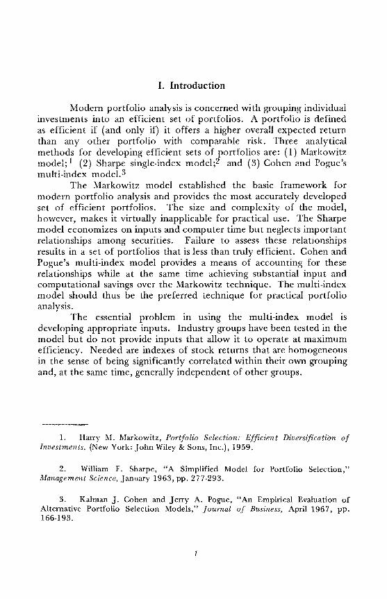
In describing the Markowitz model, it is useful to illustrate firstthe concept of efficiency by means of Figure 1. The vertical axis refersto expected return while the horizontal axis refers to risk as measuredby the variance of return (the standard deviation of return, which is

1. Cohen and Pogue actually developed two forms of the multi-indexmodel-the covariance form and the diagonal form. Both forms are quite similarand to simplify the exposition only the covariance form is analyzed.

3

FIGURE 1---THE PORTFOLIO POSSIBILITY SET

B

A

Risk-Var{R)

4

2Rp = X1 R 1 + X2R 2: L XiRi

i=lWhile the expected return of a portfolio can be obtained

directly, the variance (or risk) of a portfolio is not simply a weightedaverage of the variances of the individual securities in the portfolio.There is also a need to consider the relationship between each securityin the portfolio and every other security as measured by the covarianceof return. The method of calculating the variance of a portfolio canagain most easily be illustrated for the case of a two-security portfolio.Using Var (Ri) to represent the variance of each security, Cov (R1R2)to represent the covariance between the two securities, and again usingXi to represent the proportion that each security represents in theportfolio, the calculation of the portfolio variance (Var Rp ) is asfollows:

the square root of the variance, is used alternatively as a measure ofrisk). The shaded area represents the set of all the possible portfoliosthat could be obtained from a given group of securities. Associatedwith each possible portfolio will be a certain level of return and a cer­tain risk. Thus, each portfolio is represented by a single point in theshaded area of Figure 1.

Note that the efficient set is represented by the upper left-handboundary of this shaded area between points A and B. Portfolios alongthis efficient frontier dominate those below the line. Specifically, theseefficient portfolios offer higher return than those at an equivalent levelof risk or alternatively entail less risk at an equivalent level of return.For example, note that portfolio C, which does not lie on the efficientboundary, is dominated by portfolios D and E, which do lie on theefficient boundary. Portfolio D offers greater return than C at the samelevel of risk while portfolio E entails less risk at the same level of returnthan portfolio C.2

As noted, an efficient portfolio (or any portfolio for thatmatter) is described by the list of individual securities contained in theportfolio as well as the weighting that each security comprises in theportfolio. The estimated or expected return of the portfolio is, inturn, merely a weighted average of the expected returns of the indivi­dual securities comprising the portfolio. Calculation of the expectedreturn can be most easily illustrated for the case of a two-securityportfolio. Using (Xi) to represent the security's proportion of theportfolio and (Ri) the expected return, the expected return of theportfolio (Rp) is calculated as follows:

2. The particular portfolio that an individual investor selects from theefficient frontier depends on that investor's degree of aversion to risk. In moretechnical terms, it depends on the nature and shape of the investor's risk-retumutility function.

5

In words, the variance of the portfolio is the weighted sum ofthe variances of the individual securities plus twice the covariancebetween the two securities.

To estimate the expected return and variance of a two-stockportfolio, five estimates are needed: expected return for each stock;variance of return for each stock; and covariance of return between thetwo stocks. Generalizing to the case of N stocks, there would be needfor N return estimates, N estimates of the variance, but a total of

N(N-l)2

covariance estimates. For example, analyzing a set of 100 stocks wouldrequire 100 return estimates, 100 variance estimates, and 4,950 co­variance estimates for a total of 5,150 estimates. Note that the task ofestimation is increased considerably by the need to consider explicitlythe interrelationship among securities as represented by the covariance.This, as might be suspected, creates one of the main problems ofpractical implementation.

Given estimates of returns, variances, and covariances for thesecurities in the universe under consideration, the efficient set of port­folios is generated by means of a programming routine known asquadratic programming. A detailed description of the routine is notessential to the purpose of this study and will only be summarized asfollows. Essentially, the program is constructed to minimize the riskof a portfolio at a given level of return, i.e., develop the efficientportfolio at a given return level (say for example, at 5 percent, or 10percent or 20 percent). The program develops minimum risk portfoliosat different levels of return, in each case specifying the securities andtheir weightings in the portfolio at that level of return. Proceeding inthis fashion, the program develops a series of portfolios differing in riskand return that trace out an efficient frontier similar to the oneillustrated by the curve AB in Figure 1.

While the Markowitz model pro.vides the most complete proce­dure for developing efficient portfolios, substantial problems of prac­tical implementation emanate mainly from the overwhelming burden ofdeveloping input estimates for the model. As noted, analysis of auniverse of 100 stocks would require 5,150 different estimates. Thetask of collecting the estimates for these 5,150 statistics is furthercomplicated by the fact that few individuals are capable of estimatingsuch sophisticated measures as variances and covariances. In addition,the quantity of data require'd taxes the memory capacity of even thelargest computers.

6

Furthermore, the co-ordination of this data-gathering procedurepresents difficulties. Most securities research departments are organizedso that specialists are assigned to the coverage of an individual industryor small group of industries. In turn, this specialization means thatindividual analytical personnel generally have little knowledge of thecharacteristics of industries other than their assigned industry. Thusobtaining estimates of relationships across industries is difficult. Forexample, the electronics specialist is likely to find it difficult to assessthe degree of comovement between his assigned industry and otherssuch as the food or chemical industries.

Single-Index Model

The Sharpe single-index modification of the Markowitz modelcircumvents the difficulty of dealing with a great number of covariancesby providing a simplified method of representing the relationshipsamong securities. The fundamental concept underlying Sharpe'ssimplified approach to portfolio analysis is that the only form ofcomovement between securities comes from a common response to ageneral market index such as the Standard & Poor's (S&P) 425. Morespecifically, it is assumed that the return (Ri) on any security is deter­mined by random factors and a linear relationship with the marketindex (Rm) of the following form:

Note that this model is simply a regression equation with Birepresenting the slope coefficient and Ai representing the interceptfrom the regression. In terms of the single-index model, the slopemeasures the responsiveness of the security's return to movements inthe market, while the intercept measures the component of securityreturn that is independent of the market return. The Ci or residualterm is assumed to equal zero on average, as is standard in regressionanalysis. Most importantly, it is assumed that the residuals are un­correlated across securities, i.e., E (CiCj) :::: O. This is in keeping withthe single-index model assumption that the sole source of comoyementamong securities is due to the general market; so that once this in­fluence has been removed, the expectation is for no correlation amongthe residuals of different securities.

Given the assumption that the residuals are uncorrelated (cross­sectionally independent), the covariance between one security and anyother security in the universe (Cov RiRj) can be derived from the basicinputs to the model. Specifically, the only need is for an estimate ofeach security's market responsiveness (Bi) and an estimate of themarket variance (Var Rm ). The covariance between the two securities

7

can then be calculated according to the following formulation:

Cov R·R· = B·B· Var R1 J 1 J m

In principle, it would be possible to proceed in this fashion andcalculate the covariance for each security in the universe. However,Sharpe has noted a simplification that circumvents the need for allthese calculations and yet provides an equivalent representation of thecovariance among securities. Again, detailed discussion of this simpli­fication is not essential to this study.

As a result of eliminating the need to consider the cornovementamong securities (except that due to general market movements),the data requirements for a portfolio analysis using the Sharpe modelare substantially less than those for the Markowitz model. Only threeestimates are required for each security to be analyzed: specific return(Ai); measure of responsiveness to market movements (Bi); and thevariance of the residual return (Var Ci)' For example, analysis of auniverse of 100 securities would require only 300 estimates (threeestimates x 100 stocks). This reduction in inputs for individual securi­ties is at the cost of two additional estimates: an estimate of the return(Rm ) and variance (Var Rm ) of the market index. The net requirementof 302 estimates for the analysis is less than one-tenth the 5,150required for the full Markowitz formulation. Furthermore, the Sharpemodel has the important advantage that analysts need to provideinformation only for the securities they follow.

While Sharpe's single-index model provides a modification ofthe Markowitz model that economizes on the number of inputs as wellas computer time required to perform a portfolio analysis, the formu­lation is an oversimplification. The Sharpe model assumes that theonly effects common to all securities arise solely from general marketmovements, but there is evidence of other less significant but stillsubstantial factors affecting the returns of all securities. (In thelanguage of the single-index model, there is a significant violation ofthe specification of uncorrelated residuals). More specifically, King 3

has documented the existence of industry effects and, that otherbroader-than-industry effects which influence the returns on individualsecurities. Failure of the single-index model to incorporate theseimportant relationships is thus likely to degrade portfolio efficiency.

3. Benjamin F. King, "Market and Industry Factors in Stock Price Be­havior",Journal of Business, January 1966, pp. 139-190.

8

Multi-Index Model

Cohen and Pogue's multi-index model provides a means of in­corporating these effects into a portfolio analysis, while at the sametime achieving some substantial savings over the general Markowitzapproach. The multi-index model is similar to the single-index modelin that the return of each security under consideration is assumed to bea linear function of some index. The multi-index model, however,assumes that the universe of securities is composed of components fromseveral classes or industries and relates each security to its respectiveclass or industry rather than to one general market index. In particular,the return on each security, (Ri), is related to its class or industry,(Rk), in the following manner:

As in the case of the single-index model, this is simply a re­gression equation with Bi representing the slope coefficient and Airepresenting the intercept from the regression. The slope measures theresponsiveness of the security's return to the return on the class orindustry index, while the intercept measures the component of securityreturn that is independent of class or industry return. The Ci orresidual term is assumed to equal zero on average, as well as beingspecified to be uncorrelated across securities in the class or industry,i.e., the residual terms of the two stocks (stocks i and j) in the Sameindustry are uncorrelated, E (CiCj ) = O.

Note that the covariance between securities within a class orindustry can be derived in essentially the same fashion as for the single­index model. As a result, the comovement of companies within thesame class or industry depends solely on the response of the companiesto their class or industry index much as in the case of the single-indexmodel specification.

On the other hand, the comovement of securities from differentclasses depends on each company's response to its class or industryindex and the extent to which the classes or industries move together.The multi-index model allows explicitly for this comovement by con­sidering the covariance between industry or class indexes in much thesame manner as between securities in the Markowitz formulation.4

4. The covariance form and diagonal form of the multi-index model differin the way each specifies interaction among component industry or class indexes.The diagonal form of the multi-index model assumes that the industry or classindexes are related to one another only to the extent that the industries or classesmove with the market. The covariance form of the multi-index model captures thefun pattern of interaction between industry or class indexes, rather than assumingthey are only related through common movement with the market index.

9

Despite providing for the full covariability among class orindustry indexes, the multi-index model still allows for a substantialreduction in inputs. For example, an analysis of 100 securities thatcould be subdivided into four classes would require the followinginputs. The first need is to estimate the specific return (Ai)' measure ofresponsiveness (Bi), and the variance of residual return (Var Ci) foreach security with its respective index, or a total of 300 estimates forthe universe. The second need is to estimate the return (Rk) andvariance (Var Rk) for each of the four class indexes for an additionaleight estimates. The final need is to develop explicitly covariancesamong the four indexes or a total of six different covariances.

The net requirement for an analysis of the 100 securitiesis 314 estimates, or only slightly larger than the 302 required by thesingle-index model. It is of course substantially less than the 5,150required by the Markowitz model for the analysis of the same sizeuniverse. At the same time, it would be expected that the multi-indexmodel could incorporate into the analysis those systematic effectsamong securities neglected by the single-index model and providealmost as exact an analysis as the Markowitz model. It thus seemsthat the multi-index model would be the preferred model for practicalportfolio analysis.

10

III. Empirical Test and Multi-Index Model Inputs

As noted in the introductory remarks, the major problem inimplementing the multi-index model has been in developing appropriateinputs. Cohen and Pogue used industry indexes as inputs to the modeland tested its performance against that of the Markowitz model andsingle-index model. The multi-index model failed, however, to outper­form the single-index model because of some basic deficiences of theindustry indexes as inputs to the model.

This section describes the Cohen and Pogue empirical test ingreater detail and also explains the problems of using industry indexesas inputs to the multi-index model.

This section also reviews the work of Benjamin King on factorsexplaining the returns of common stocks. This study was importantbecause it provided empirical support for the use of index models forpurposes of portfolio selection. The study confirmed that the generalmarket factor is highly important in explaining the returns of commonstocks and thus provided support for the use of the single-index model.Correspondingly, the study showed that industry factors can be impor­tant in explaining common stock returns and provided support for theuse by Cohen and Pogue of industry indexes as inputs to the multi­index model.

While the King study showed the importance of these twofactors (market and industry) in explaining common stock returns,indications from the study itself show the need for an additionalbroader-than-industry factor to explain more completely commonstock returns. The remainder of this section discusses some potentialbases for introducing an additional factor for explaining stock returns.The section concludes by noting that grouping stocks according togrowth, cyclical, and stable characteristics provides the most promisingbasis for developing a broader-than-industry factor for explainingstock returns.

Empirical Evaluation of Portfolio Selection Models

Cohen and Pogue l tested the Markowitz, single-index, andmulti-index models to determine the relative efficiency of each inselecting optimum portfolios on both an ex-ante and ex-post basis.

1. Cohen and Pogue, op. cit.

11

The authors utilized historical returns, variances, and covariance8among individual stocks as inputs to the Markowitz model. Historicalmarket returns and variances of return as well as historical relationshipsof individual stocks with the market (i.e., historical Ai, Bi, and VarCi values) were used as inputs to the single-index model. Cohen andPogue utilized ten industries classified by traditional industry classifi­cations (two-digit S.LC. codes) as indexes for the multi-index model.Again, historical industry returns and variances of industry returns aswell as historical relationships of stocks with the industry indexes (i.e.,historical Ai, Bi, and Var Ci values) were used as data inputs to themulti-index models.

The test indicated essentially that the multi-index model didnot provide the expected improved performance over the single-indexmodel on either an ex-ante or ex-post basis. Specifically, Cohen andPogue found in their evaluation of these models that the ex-anteefficient frontiers generated by portfolios using the single-index modeldominated those generated by the multi-index model. In addition, theauthors found that the ex-post performance of the index models wasnot dominated by the Markowitz formulation, and that the perfor­mance of the multi-index model was not superior to that of the single­index formulation.

Cohen and Pogue attributed this difference in performance ofthe models to the relative ability of each to reproduce the true co­variance between individual security returns. The authors obtaineda measure of this relative ability by comparing the correlation matriximplied by the index models with the true correlation matrix used inthe Markowitz model. They found that while the multi-index modelmost closely represented the true correlations among securities withinthe same industries, the relationships among securities in differentindustries were somewhat better represented by the single-index model.Because of the much larger number of inter-industry as opposed tointra-industry comparisons among companies in the sample, the single­index model was found, on the average, to represent better the truecorrelation matrix.

While Cohen and Pogue's study showed that the single-indexmodel dominated the multi-index model using traditional industrycategories as inputs, these results do not necessarily lead to the con­clusion that the single-index model is preferable to the multi-indexmodel. The main implication is that industry indexes are basicallydeficient as inputs to the multi-index model. Specifically the indexesused in the study showed high inter-index correlation even after

12

removal of the general market effect from each index.2 Use of suchhighly collinear inputs does not allow the multi-index model to operateat maximum efficiency.

Indexes of stocks are needed that are homogeneous in the sensethat they are significantly correlated within their own grouping and, atthe same time, independent of other groups.3 Use of such non-corre­lated indexes in the multi-index model should lead to a more accuratelyrepresented covariance matrix and thereby a set of efficient portfoliossuperior to the single-index model. As noted earlier, it is a majorpurpose of this study to develop stock groupings that are homogeneouswith respect to coHinearity characteristics.

Market and Industry Factors

Before discussing the basis for developing such groupings, itwould be useful to review the empirical work of Benjamin King con­cerning market and industry factors explaining the price behavior ofcommon stocks.4 King's study hypothesized that the change in the logprice of a common stock is the weighted sum of a market, an industry,and a company effect. This hypothesis was based on the observationthat investors commonly refer to market-wide or industry-wide pricemovements of securities; and that companies are typically classifiedaccording to industries. King further noted that a widely used methodof industry classification was that of the Securities and ExchangeCommission and correspondingly desired to test whether a potentialindustry effect would correspond to the two-digit S.LC. classifications.

In order to test these hypotheses, King selected a sample of63 common stocks classified into the following six two-digit S.LC.industries: (1) Tobacco products; (2) Petroleum products; (3) lVleta1s(ferrous and non-ferrous), (4) Railroads; (5) Utilities; and (6) Retailstores. King then utilized factor analysis to examine the covariationof these 63 common stocks over the 1927-60 period. This analysis in­dicated that general market effects accounted for roughly 50 percentof the variance in a security's log price over the full period of the study.Industry effects accounted for approximately 10 percent of the vari­ance in log price. The 40 percent remainder of the variance wasascribed to effects unique to an individual security. The stock group-

2. This correlation is noted in table 3 on page 177 of the Cohen and Poguestudy showing the frequency distribution of the correlation coefficients of residualsfor the ten industry indexes. This table indicates that 40 percent of the residualsshowed positive correlation with approximately 15 percent of the residual pairingsexhibiting correlation coefficients of 0.50 or larger.

3. Independent in the sense that the residuals of these indexes (after re­moval of the general market effect) display no correlation.

4. King, op. cit.

13

ings that emerged from the analysis of stock price behavior corres­ponded to the hypothesized two-digit S.Le. industry classifications.

While King's results indicate that market and industry effectsare important factors explaining the change in stock prices, indicationsare that the three effects-market, industry, and company-may notbe a sufficient number to account for the complex interrelationship ofsecurity price changes. First, an .analysis of four subperiods by Kingindicated a successive decline in the importance of the market factorover the total period of the study, as may be noted by the followingsubperiod statistics: (1) 58 percent, 1927-35; (2) 56 percent, 1935­1944; (3) 41 percent, 1944-52; (4) 31 percent, 1952-60. The declinein the importance of the market factor was also detected in Blume'sstudy. 5 Blume, using regression analysis, found that a market indexaccounted for an average of 47 percent of the variability of monthlyreturns on 251 securities over the 1927-60 period, but that the pro­portion of explained variance declined in each of successive quarternsfrom 53 percent, to 50 percent, to 38 percent, and finally to 26 per­cent. This non-stationarity over time of the market effect led King tosuggest that other factors may be important in explaining the price ofcommon stocks as reflected by the following statement: "Hence theapparent diminution of the influence of the market implies an increasein relative importance of the unique parts of the variance, or at leastthose parts that are explained by factors in addition to market andindustry:"6

In addition, the cluster analysis employed by King indicatedthat some industry groupings showed sufficient correlation to warrantpossible consideration as single rather than separate clusters.7 Thiscorrelation among industry groups could be noted from the fact thatthe cluster procedure continued for several passes after the six hypothe­sized industries had emerged on the 56th pass of the routine. Forexample, King's results showed a clustering of the tobacco and retailindustries at a positive correlation between 0.15-0.20 and a furtherclustering of this group with the utility industry at a positive corre­lation between 0.10-0.15. In addition, the rails and metals industriesclustered together with a positive correlation coefficient between 0.10-­0.15. The cluster routine then terminated at the 59th pass (no furtherpositive correlations) to provide three separate groups: (1) oil industry;(2) rail and metal industries cluster; and (3) tobacco, retail, and utilityindustries cluster.

5. Marshall Blume, "Assessment of Portfolio Performance: An Applica­tion of Portfolio Theory," (unpublished dissertation), March 1968.

6. King,op. cit., p. 157.

7. King,op. cit., p. 153.

14

Finally, an analysis of the correlations among industry factorsfor the overall 1927-60 period as well as four subperiods showed somesignificantly positive correlation among separate industry factors.8

Specifically, the tobaccos and stores factors showed positive correlationin two out of four subperiods and for the overall period showed a corre­lation of +0.25 which is highly significant statistically for a samplewith 403 observations. With the exception of the first subperiod, thetobacco and utility industry factors showed positive correlation thatwas generally statistically significant. Utilities and stores showed pos­itive correlation in two out of four subperiods. Finally, metals andrails showed positive correlation in three out of four subperiods.

As in the case of the cluster analysis, the positive correlationamong the utilities, stores, and tobacco factors, as well as the rails andmetals factors, indicates the possibility that two separate groups mightbe formed from these five industries. In addition, the predominantlynegative correlation among these groups, as well as with the oil indus­try, indicates that it might be possible to form a total of three separategroups from the six industries analyzed by King. These results, in con­junction with the cluster analysis results, again suggest the possibilitythat anothe; factor-broader than the industry factor and in addition tothe market and company factors-is needed to explain the variation inlog prices of common stocks.

Potential Additional Factor

While the preceding analysis of King's factor analysis results issuggestive of the need for a factor in addition to those of market,industry, and company, the most appropriate basis on which tointroduce an additional factor is not immediately apparent. King'smethod of amalgamating companies to form industry factors suggestsamalgamating industry factors to form group factors. Accordingly, wefirst consider the potential for classifying stocks according to severalmore conventional economic methods and then describe a method thatseems to be the most promising for developing an additionalbroader-than-industry factor for grouping stocks.

Several more conventional methods for classifying companies orindustries by economic characteristics are: (1) dependence on a certaincategory of spending such as consumer spending, business (capital)spending, or government spending; (2) product similarity such asdurable or nondurable goods; or (3) stage in the manufacturing cyclesuch as raw material, intermediate, or final product. Due to theseeconomic similarities, it might be expected that the earnings patterns

8. King,op. cit., p. 156.

15

of companies within the same economic categories would behavesimilarly. The extent to which the prices of stocks coincided with thecompany's earning pattern would then determine the degree to whichthe covariation of stocks could be attributed to economic character­istics of companies.

A paper by Granger and Morgenstern9 is relevant to the subjectof the extent to which price patterns of stocks adhere to such methodsof classification. Granger and Morgenstern used cross-spectral methodsto analyze price indexes and, to a limited extent, to analyze the pricebehavior of individual stocks. The most pertinent result for purposesof this study is the report on the coherences among changes in theseveral component indexes (mainly series categorized by economiccharacteristic) of the S.E.C. Weekly Composite Index (1939-61). Thecoherence is defined as an index of association between componentsat the same frequency for two series.

The results of the authors' analysis were consistent withexpectations in the cases where price series such as (1) manufacturingand durable goods, (2) durable goods and motor vehicles, (3)transportation and rails showed a high degree of covariation, whileseries such as (1) manufacturing and utilities, (2) utilities and mining,and (3) mining and trade, finance and services showed an expected lowdegree of covariation. However, the low degree of covariation amongthe following series was contrary to expectation: (1) durable goods andradio, television, and communications equipment; (2) motor vehiclesand radio, television, and communications equipment; (3) transporationand air transportation. The evidence concerning the covariation of priceseries according to these economic classifications was thus mixed, asthere were almost as many instances of price series moving in anunexpected direction as there were series showing the expected degreeof covariation.

A paper by Feeney and Hester 10 is also relevant to the classi­fication of security price covariation according to economic characteris­tics. Feeney and Hester utilized principal components analysis to studythe 30 component stocks of the Dow Jones Industrial Average for non­overlapping quarters during the period 1951-63. The authors extractedthe first two principal components from the following three matrices;0) covariance matrix; (2) correlation matrix; and (3) correlation matrixwith the time trend in the original data removed. -

An examination (by the authors) of the signs and weights ofthe components derived from these three matrices indicated that the

9. C.W.]. Granger and O. Morgenstern, "Spectral Analysis of New YorkStock Market Prices," Kyklos, 1963, pp. 1-27.

10. G.]. Feeney and Donald Hester, "Stock Market Indices: A PrincipalComponents Analysis," (unpublished preliminary paper), 1964.

16

following DJI stocks showed a relatively high degree of similarity:AT&T, Eastman Kodak, General Foods, Procter and Gamble, Sears,and Woolworth. Feeney and Hester noted that these stocks were per­haps the most consumer oriented of the Dow Jones stocks and con­jectured that the extracted components discriminated betweenproducer and consumer goods industrial stocks. The authors speculatedthat an explanation for such a phenomenon might be that profits ofproducer goods firms and consumer goods firms reach peaks atdifferent points in a business cycle. A simple accelerator model mightyield such a result. 11

The existence of a potential accelerator effect in the data was,however, only partially substantiated as the producer oriented stockssuch as Anaconda, Bethlehem Steel, International Paper, and Swift(Esmark) did not display a high degree of similarity across extractedcomponents. Also, in order for such an accelerator effect to hold true,it must be assumed that stock prices are closely related to currentearnings; the use of reported earnings rather than expected earnings inempirical tests of cost of capital models has been a source of criticism.Finally, Feeney and Hester's conjecture of an accelerator effect wasbased entirely on a preliminary examination of the data and no effortwas made (on the part of the authors) to carry this analysis further.As in the case of the Granger and Morgenstern analysis, the existenceof a grouping of stocks by these more conventional economic classifi­cations is not strongly supported.

While tests of these more conventional methods of economicgrouping have not been fruitful, one that is untested and yet seemspromising is grouping stocks according to growth, cyclical and stablecharacteristics. Investors generally consider growth stocks to be repre­sented by companies expected to show an above average rate of secularexpansion. Cyclical stocks are defined as those of companies that havean above average exposure to the vagaries of the economic environ­ment. Earnings of these companies are expected to decline more thanaverage in a recession and to increase more than average during anexpansion phase of the business cycle. Stable stocks are those of com­panies whose earning power is less affected than the average companyby the economic cycle. Earnings of these companies are expected toshow a below average decline in a recession and a less than averageincrease during the expansion phase of the business cycle.

11. l"eeney and Hester, op. cit., p. 22.

17

IV. Empirical Test of Stock Grouping Hypothesis

This section tests whether the price action of stocks conformsto classes of growth, cyclical, and stable stocks.! The criterion forjudging whether stock price movements conform to this method (orany other for that matter) is a high degree of association between theprice movements of stocks within a class and a low degree ofassociation with other classes of stocks. More specifically, growthstocks would be expected to be highly related to other growth stocks,cydicals with other cydicals, and stables with stables, but growthstocks should be unrelated to cydicals and stables, and these in turnshould be unrelated to each other. Should groups of stocks meet thiscriterion, it would be appropriate to add a broader-than-industry factorto the market and industry factors previously determined by King.

Selection of Test Sample

To test whether stocks group according to this broader-than­industry method of classification, a sample of 100 common stocks wasselected for analysis (Table 1). These 100 companies represent 60separate Standard & Poor's industry classes and 25 of the two-digitS.Le. categories. All are listed on a national exchange, and 90 of thecompanies are included in the Standard & Poor's 500 Index. The totalcapitalization of this sample of 100 companies represents approxi­mately 50 percent of the market value of the S&P 500. Finally, allindustrial companies in the sample are included in Fortune's 500largest industrial enterprises, with the smallest company listed 300thin sales and 400th in assets.

The majority of stocks in the sample of 100 fell readily intoone of the three hypothesized stock categories. For example, tech­nologically-oriented companies, such as those in the electronics andoffice equipment areas, were easily classified as growth stocks.Machinery companies and other heavy equipment manufacturing cate­gories were clearly cyclical stocks, while consumer-oriented companiessuch as foods and utilities displayed stable characteristics. Categories

1. This section essentially reviews material from James L. Farren, Jr.,"Homogeneous Stock Groupings: Implications for Portfolio Management,"Financial Analysts Journal, May-June 1975. Those familiar with this article mayonly wish to briefly review this section and proceed to the next section.

18

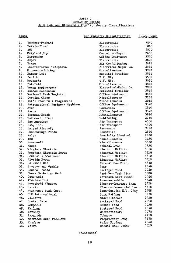
Table 1Sample of Stocks

By S.I.C. and Standard & Poor's Industry Classifications

S&P Industry Classification S.Le. Code

1. Hewlett-Packard2. Perkin-Elmer3. AMP4. Maryland Cup5. Burroughs6. Ampex7. Trane8. International Telephone9. Minnesota Mining10. Baxter Labs11. Zenith12. Motorola13. Polaroid14. Texas Instruments15. Becton-Dickinson16. National Cash Register17. Corning Glass18. Int'l Flavors & Fragrances19. International Business Machines20. Avon21. Xerox22. Eastman-Kodak23. Harcourt, Brace24. Pan American25. UAL, Inc.26. United Aircraft27. Chesebrough-Ponds28. Nalco29. TRW30. Honeywell31. Merck32. Virginia Electric33. American Electric Power34. Central & Southwest35. Florida Power36. Columbia Gas37. Procter and Gamble38. General Foods39. Chase Manhattan Bank40. Coca-Cola41. Transamerica42. Household Finance43. C.l.T.44. Northwest Bank Corp.45. epe International46. Gillette47. Quaker Oats48. Campbell49. Kellogg50. Hershey51. Reynolds52. American Home Products53. Kraftco54. Sears

(continued)

19

ElectronicsElectronicsElectronicsContainer-PaperOffice EquipmentElectronicsAir-ConditioningElectrical-Major Co.MiscellaneousHospital SuppliesT.V. Mfg.T.V. Mfg.MiscellaneousElectrical-Major Co.Hospital SuppliesOffice EquipmentMiscellaneousMiscellaneousOffice EquipmentCosmeticsOffice EqUipmentMiscellaneousPublishingAir TransportAir TransportAerospaceCosmeticsSpecialty ChemicalMiscellaneousMiscellaneousEthical DrugElectric UtilityElectric UtilityElectric UtilityElectric UtilityNatural Gas Diat.SoapPackaged FoodBank-New York CityBeverage-Soft DrinkInsurance-LifeFinance-Consumer LoanFinance-Commercial LoanBank-Outside N.Y. CityCorn RefinerMiscellaneousPackaged FoodCanned FoodPackaged FoodConfectionaryTobaccoProprietary DrugDairy ProductRetail-Mail Order

38403840387026503570367036153650399038303630363038103880383035103250201535702880.359038102710450045003720288028303750382028.3058105810581058105830284020505580208655405520551055803430343020502030205020702110283020605310

Stock

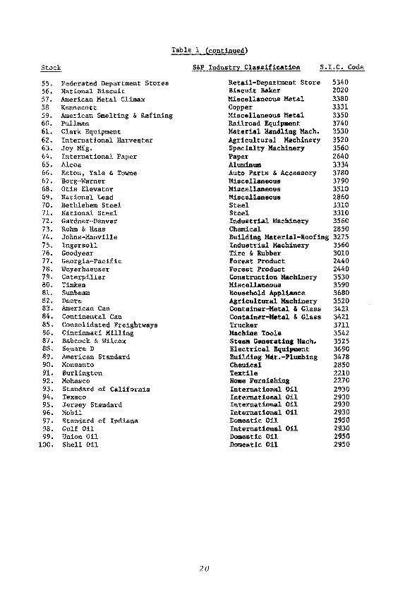
Table 1 (continued)

S&P Industry Classification S.LC. Code

55.56.57.5859.60.61­62.63.64.65.66.67.68.69.70.71.72.73.74.75.76.77.78.79.80.81.82.B3.84.85.86.87.88.89.90.91.92.93.94.95.96.97.98.99.

100.

Federated Department StoresNational BiscuitAmerican Metal ClimaxKennecottAmerican Smelting & RefiningPullmanClark EquipmentInternational HarvesterJoy Mfg.International PaperAlcoaEaton, Yale & TowneBorg-WarnerOtis ElevatorNational LeadBethlehem SteelNational SteelGardner-DenverRohm & HaasJohns-ManvilleIngersollGoodyearGeorgia-PacificWeyerhaeuserCaterpillarTimkenSunbeamDeereAmerican CanContinental CanConsolidated FreightwaysCincinnati MillingBabcock &WilcoxSquare DAmerican StandardMonsantoBurlingtonMohascoStandard of CaliforniaTexacoJersey StandardMobilStandard of IndianaGulf OilUnion OilShell Oil

20

Retail-Department StoreBiscuit BakerMiscellaneous MetalCopperMiscellaneous MetalRailroad EquipmentMaterial Hand1:l.ng Mach.•Agricultural MachinerySpecialty MachineryPaperAlUlllinUlllAuto Parts &AccessoryMiscellaneousMiscellaneousMiscellaneousSteelSteelIndustrial MachineryChemicalBuilding Material-RoofingIndustrial MachineryTire & RubberForest ProductForest ProductConstruction MachineryMiscellaneousHousehold ApplianceAgricultural MachineryContainer-Metal &GlassContainer-Metal &GlassTruckerMachine ToolsSteam Generatina Mach.Electrical EquipmentBuilding ~t.-PIUlllbing

ChemicalTextileHome FurnishingInternational OilInternational OilInternational OilInternational OilDomestic OilInternational OilDomestic OilDomestic 011

5340202033803331335037403530352035602640333437803790351028603310331035602850327535603010244024403530359036803520342134213711354235253690347828502210227029302930293029302950293029502950

for certain other groups of stocks-such as airlines and television, thatcould fit either growth or cyclical classes and soft drinks that could beeither growth or stable-resisted classification. Finally, some investorsbelieve that stocks of certain industries, such as construction or aero­space, may display unique price behavior because of their economiccharacteristics, thereby creating stock groupings independent of thoseoriginally hypothesized.

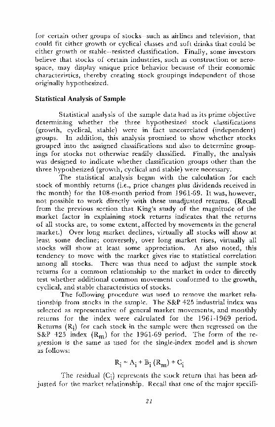
Statistical Analysis of Sample

Statistical analysis of the sample data had as its prime objectivedetermining whether the three hypothesized stock classifications(growth, cyclical, stable) were in fact uncorrelated (independent)groups. In addition, this analysis promised to show whether stocksgrouped into the assigned classifications and also to determine group­ings for stocks not otherwise readily classified. Finally, the analysiswas designed to indicate whether classification groups other than thethree hypothesized (growth, cyclical and stable) were necessary.

The statistical analysis began with the calculation for eachstock of monthly returns (i.e., price changes plus dividends received inthe month) for the lOS-month period from 1961-69. It was, however,not possible to work directly with these unadjusted returns. (Recallfrom the previous section that King's study of the magnitude of themarket factor in explaining stock returns indicates that the returnsof all stocks are, to some extent, affected by movements in the generalmarket.) Over long market declines, virtually all stocks will show atleast some decline; conversely, over long market rises, virtually allstocks will show at least some appreciation. As also noted, thistendency to move with the market gives rise to statistical correlationamong all stocks. There was thus need to adjust the sample stockreturns for a common relationship to the market in order to directlytest whether additional common movement conformed to the growth,cyclical, and stable characteristics of stocks.

The following procedure was used to remove the market rela­tionship from stocks in the sample. The S&P 425 industrial index wasselected as representative of general market movements, and monthlyreturns for the index were calculated for the 1961-1969 period.Returns (Ri) for each stock in the sample were then regressed on theS&P 425 index (Rm ) for the 1961-69 period. The form of the re­gression is the same as used for the single-index model and is shownas follows:

R· :::: A· + B· (R ) + c·I I I m I

The residual (Ci) represents the stock return that has been ad­justed for the market relationship. Recall that one of the major specifi-

21

cations of the single-index model is that these residuals should be un­correlated, that is E (CiCj) =: O-i.e., that the sole source of comovementamong stocks is their relationship to the general market. Hence, a testfor residual correlation according to growth, cyclical, and stable charac­teristics is in a sense a test of the validity of the single-index modelspecification of uncorre1ated residuals.

Once returns had been adjusted for the market relationship,a coefficient of correlation was calculated between each stock in thesample and every other stock. Recall that the coefficient of correlationis a statistical measure of association between two stocks ranging invalue between +1 and _1.2 With 100 stocks in the sample and each

n9l.J.B.U.~atrix.E!_c.,,-rr_elati.~ .. C:,,-efficillr1-!S_GrO\"/!-h~~.c:Iic!,IL~~ Sta~Ie.!)tock~

GROWTH CYCLICAL STABLE

GROWTH

CYCLICAL

STABLE

GROWTH L LSTOCKSH+

L CYCLICAL LSTOCKSH+

_._----~._-----_..._-----_._-_ ..__...._...

, STABLE

L L STOCKSH+

2. Two secuntles with perfectly correlated return patterns will have acorrelation of +1. Conversely, if the return patterns are perfectly negatively corre­lated, the correlation coefficient will equal -1. Two securities with uncorrelated(i.e., statistically unrelated) returns will have a correlation coefficient of zero. Thecorrelation coefficient between returns. for securities in this sample and the S&P425 Market Index during the 1961-69 period was generally between 0.5 and 0.6.

22

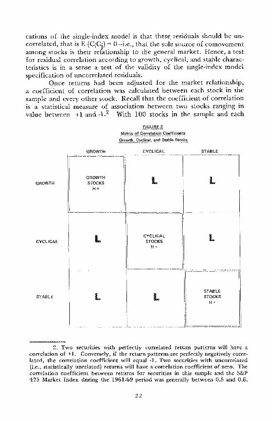
being correlated with every other, the result is (100 x 100) == 10,000correlation coefficients.

If stocks in fact group according to growth, cyclical, and stablecharacteristics, we would expect them to exhibit the pattern of highcorrelation within groups and low correlation across groups that isillustrated by the matrix of correlation coefficients in Figure 2. Speci­fically, the correlation coefficients within each of the classes--growth,cyclical and stable stocks, arranged along the diagonal of the matrix­should show high and positive values. These are identified within eachof the groupings by the letter H and a plus sign. The correlationcoefficients 9ff the diagonal represent the correlation of stocks betweengroups (growth with cyclical, cyclical with stable, etc.), and are expect­ed to be low in value. These are identified by the letter L.

Cluster Analysis

The test whether the sample stocks in fact showed the expectedpattern is based on a statistical technique known as duster analysis,which systematically examines the matrix of correlation coefficients.3The duster analysis technique separates stocks into groups or clusterswithin which stocks are highly correlated, and between which stocksare poorly correlated. It is a stepwise process that involves (1) searchingthe correlation matrix for the highest positive correlation coefficient;(2) combining these stocks to reduce the matrix by one; and (3) recom­puting the correlation matrix to include the correlation between thecombined stock or duster and the remaining stocks or dusters. Thisprocess continues in an iterative fashion until all positive correlationcoefficients are exhausted or until (on the 99th pass) every stock isformed into a single duster.

If the hypothesis that the 100 stocks in the sample could becategorized were correct and if the individual stocks were correctlyclassed, then by the 97th pass the three remaining groups shouldcorrespond to those hypothesized. Furthermore, all positivecorrelation coefficients should be exhausted by the 97th pass, thusterminating the process. This result would indicate, not only that thesample data can be explained by three independent groupings, but alsothat there is a low degree of correlation across stock groupings.

3. The cluster technique used in this study is similar to one used by King,op. cit., and termed a "quick and dirty" method of factor analysis. King viewedthe routine as a method of exploration properly falling under the heading of "dataanalysis" rather than "inference," the results of which would be subject to testingand confirmation via other techniques. 'Dle cluster results in this study were, infact, confirmed by other tests reported in an article by James L. Farrell, Jr., "An­alyzing Covariation of Returns to Determine Homogeneous Stock Groupings,"Journal of Business, April 1974, pp. 181-207.

23

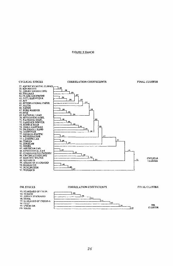
Figure 3 provides a set of four diagrams showing the results ofthe duster routine. The diagrams show the stage where pairs or groupsof stocks joined, along with the value of the correlation coefficient atwhich they joined. Describing the duster results required four dia­grams, because an oil group emerged from the analysis in addition tothe three groups originally hypothesized (the routine terminated on the96th pass as no positive correlation coefficients remained at that stage).Actually, it had originally been expected that oils would group with thestable category of stocks, but the oil cluster failed to show a positivecorrelation with the stable cluster (or any other, for that matter).4No other independent groups emerged from the cluster analysis. Theaerospace and building stocks--that might have been expected toexhibit independent behavior-clustered with the growth and cyclicalgroups respectively.

The number of stocks in each cluster is: growth, 31; cyclical,36; stable, 25; and oil, 8. Stocks that. had been given an a prioriclassification of growth, stable or cyclical actually clustered with theirallocated groups. Naturally, all oil stocks clustered together. Thosestocks that were not easily classified on an a priori basis--such as tele­vision, airlines and soft drinks-generally clustered with a group thatcould be accepted as reasonably appropriate. All group clustersappeared to contain highly intercorrelated stocks; final stocks or groupof stocks clustering into individual groups did so at relatively high levelsof positive correlation: 0.19, growth; 0.15, stable; 0.18, cyclical; and0.27, oil. The final four groups were not positively correlated, asevidenced by the fact that the routine terminated on the 96th pass(positive correlation of 0.15 was the lowest positive correlation on theprior, 95th pass).

Index Procedure

To determine the degree of pOSItIVe correlation of stockswithin each of the four groupings of growth, cyclical, stable and oilstocks as well as the extent to which stocks were uncorrelated withthose of other groupings, the author developed first a rate of return(adjusted for general market effects) for each of the four stock group­ings. Stocks that clustered into the four groups were formed directlyinto four monthly indexes composed of (1) 31 growth stocks, (2) 25

4. Recall that King's results indicated that the oil industry was also theonly one that showed no positive correlation with any of the other five industriesanalyzed and is further evidence that the oil group is sufficiently unique to beconsidered an independent category.

24

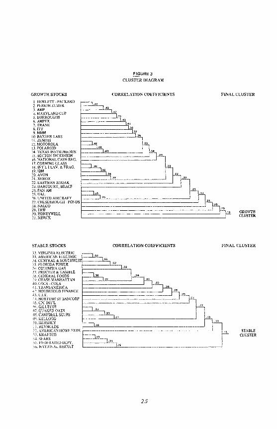
FIGURE 3

CLUSTER OIAGRAM

FINAL CLUSTERGROWTH STOCKS

I. HEWLETT· PACKARD2. PERKIN ELMER3.AMP4. MARYLAND CUP5. BURROUGHS6. AMPEX7. TRANE8. ITT9.MMM

10. BAXTER LABSII.ZENiTH12. MOTOROLA13. POLAROID14. TEXAS INSTRUMENTS15. BECTON DICKINSON16. NATIONAL CASH REG.17. CORNING GLASSIS.INrL FLAV.& FRAG.19. IBM20. AVON21. XEROX22. EASTMAN KODAK23. HARCOURT, BRACE24. PAN AM25. UAL26. UNITED AIRCRAFT27. CHESEBROUGH - PONDS28. NALCO29. TRW30. HONEYWELL31. MERCK

CORRELATION COEFFICIENTS

----'.41

.4'

----~..38

.43

.41.3.

.31

.35

~. Jh~.40.43 .34

.33

n.3.

[h-3..34 .32

.31 .32

==:=ill,

~.28

.35

-"_ .20

.1'- .1' GROWTH

CLUSTER

STABLECLUSTER

FINAL CLUSTER

.1'

.17

.33

.21

CORRELAnON COEFFICIENTS

.23

.32

.32

.35

.53

STABLE STOCKS

32. VIRGINrA ELECTRIC33. AMERICAN ELECTRIC34. CENTRAL & SOUTHWESlf- ..J.:.:·5;:.5,

35. FLORIDA POWER .52

36. COLUMBIA GAS37. PROCTER & GAMBLE38. GENERAL FOODS39. CHASE MANHATTAN40. COCA -COLA41. TRANSAMERICA42. HOUSEHOLD FINANCE43. C.I.T.44. NORTlIWFST BANCORP45. CPC INrL46. GILLETTE·17. QUAKER OATS4S. CAMPBELL SOUPS·~IJ. KELLOGG'O.IILRSHEY .17

51. REYNOLDS }SC. AMERICAN HOME PRDS. f-------.-------------------'53. KRAFTCO .15

54. SEARS55. FEDERATED DEIYf.5<,. NATIONAL BISCUIT

25

CYCLICAL STOCKS

57. AMERICAN METAL CLIMAX58. KENNECOTT59. AMERICAN SMELTING60. PULLMAN61. CLARK EQUIPMENT62. INT'L HARVESTER63. JOY64. INTERNATIONAL PAPER65. ALCOA66. EATON67. BORG WARNFR68.0TlS69. NATIONAL LEAD70. BETHLEHEM STEEL71. NATIONAL STEEL72. GARDNER DENVER73. ROHM & HAAS74. JOHNS MANVILLE75. INGERSOLL RAND76. GOODYEAR77. GEORGIA PACIFIC78. WEYERHAUSER79. CATERPILLAR80. TlMKEN81. SUNBEAM82. DEERE83. AMERICAN CAN84. CONTINENTAL CAN85. CONSOLIDATED FREIGHT86. CINCINNATl MILLING87. BABCOCK WILCOX88. SQUARE D89. AMERICAN STANDARD90. MONSANTO91. BURLINGTON92. MOHASCO

OIL STOCKS

CORRELATION COEFFICIENTS

:=12; .38.3.

--,- .36

n~.36 .25

.2'

--, .3.~

.33.34

r---. ...~

.42.3.

.3' ~.37.30

r--l.3. .21

r----. 5 r-.32

~.'7~.37

.3'.2'

.23

r----, .2.

2..27

CORRELATION COEFFICIENTS

FINAL CLUSTER

CYCLICALCLUSTER

FINAL CLUSTER

93. STANDARD OF CALIF.

94. TEXACO ~~'55~~95. JERSEY STANDARD ~_ 1.56

96. MOBIL 1.5197. STANDARD OF INDIANA 1.5.

;;~ ~~~(~N OIL 155 I",100. SIIELL

26

1.30OIL

CLUSTER

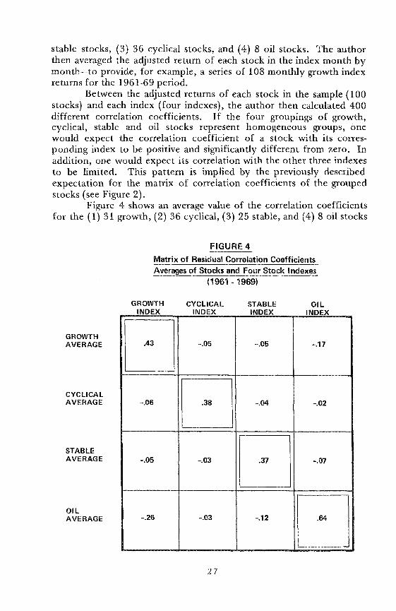
stable stocks, (3) 36 cyclical stocks, and (4) 8 oil stocks. The authorthen averaged the adjusted return of each stock in the index month bymonth--to provide, for example, a series of 108 monthly growth indexreturns for the 1961-69 period.

Between the adjusted returns of each stock in the sample (100stocks) and each index (four indexes), the author then calculated 400different correlation coefficients. If the four groupings of growth,cyclical, stable and oil stocks represent homogeneous groups, onewould expect the correlation coefficient of a stock with its corres­ponding index to be positive and significantly different from zero. Inaddition, one would expect its correlation with the other three indexesto be limited. This pattern is implied by the previously describedexpectation for the matrix of correlation coefficients of the groupedstocks (see Figure 2).

Figure 4 shows an average value of the correlation coefficientsfor the (1) 31 growth, (2) 36 cyclical, (3) 25 stable, and (4) 8 oil stocks

FIGURE 4

Matrix of Residual Correlation CoefficientsAverages of Stocks and Four Stock Indexes

(1961 - 1969)

GROWTHINDEX

CYCLICALINDEX

STABLEINDEX

OILINDEX

GROWTHAVERAGE

CYCLICALAVERAGE

STABLEAVERAGE

OILAVERAGE

[J -.05 -.05 -.17

-.06 [J -.04 -.02

-.05 -.03 [J -.07

-.26 -.03 -.12 D27

with the corresponding index as well as with the other three indexes(this 4 x 4 matrix thus summarizes the full 4 x 100 correlation matrixof stocks and indexes). The average values of the correlation coeffi­cients of stocks with the corresponding index were all positive andhighly significant (correlations of 0.19 or higher occur by chance onlyone time in 20). At the same time, the average values of the corre­lation coefficients of stocks with other indexes indicated a low degreeof correlation.

In addition, inspection of the complete correlation matrix ofstocks and indexes (complete matrix not specifically shown) indicatedthat each stock included in the group average was positively correlatedwith its respective index at a statistically significant leveL Specifically,all growth stocks were positively and significantly correlated with thegrowth index, as were stable stocks with the stable index, cyclicals withthe cyclical index, and oils with the oil index. Only six stocksshowed significantly positive correlation with an index other than theone assigned and in each case the stock was more highly correlated withits assigned index. With the exception of these six stocks, all othersdisplayed either negative correlation or less than significant positivecorrelation with indexes other than the index for their own groupings.It is hard to avoid the conclusion that growth, cyclical, stable, and oilstocks do in fact represent homogeneous groupings.

Significance of Group Effects

One can use regression analysis to determine the percentage ofthe observed variations in return on the individual stock explained bysuch systematic factors as market, or growth, cyclical, stable, and oiLThis study used the S&P 425 Index to represent the general marketfactor, while the previously described indexes of adjusted returns wereused to represent growth, cyclical, stable, and oil factors. The coeffi­cient of determination (R2) from the regression is an estimate of thepercentage of realized returns of individual stocks explained by system­atic factors.

The average R 2 for all stocks in the sample 100 with that of themarket over the 1961-69 period was approximately 30 percent, whichis consistent with the figures in other studies (including King's) of thepostwar period. The average R 2 from the regression of the return ofthe individual stock on the adjusted return of the corresponding index(i.e., growth stock on growth index; cyclical on cyclical index; stable onstable index; and oil on oil index) for the same 1961-69 period wasapproximately 15 percent. These two systematic factors combinedthus account for approximately 45 percent of the realized return of an

28

~ndividual stock, with the remainder attributable to the industry factoror effects unique to the individual security.5

As this completes the test of the stock grouping hypothesis,it would be useful at this point to emphasize the main findings of thissection. It is that four groupings of stocks (growth, cyclical, stable,and oil) are homogeneous in the sense of being highly correlated withingroupings and not significantly correlated with other stock groupings.These four groupings in turn represent a broader-than-industry factoradditional to' the market and industry factors previously determinedby King. Correspondingly, these groupings that are homogeneous withrespect to collinearity characteristics provide a suitable means fordeveloping inputs to the multi-index portfolio selection model.

5. Recall that King showed that the industry factor accounted for 10 per­cent of the realized return of common stocks during the 1927-60 period. Adding10 percent for industry effects (under the assumption that this effect has continuedto maintain a reasonable degree of stability over time) to the 45 percent of theother two systematic factors indicates that these three effects may explain 55 per­cent of the realized return of common stocks. This would in turn indicate thateffects unique to a security are somewhat less than 50 percent.

29

v. Test of Relative Performance of Multi-Index Model

This section describes a test of the performance of the multi­index model using indexes constructed from homogeneous groups ofgrowth, cyclical, stable and oil stocks. The test includes an analysis ofthe facility of both the multi-index and single-index models in generat­ing ex-ante efficient sets of portfolios as well as a comparison of theperformance of these efficient portfolios to that of the S&P 500 anda set of mutual funds over an ex-post period. The final part of thepaper analyzes the stability of input relationships to the model. Thisanalysis is important in indicating the extent to which historic data canbe used in the practical application of the model.

Analysis of Index Model Specifications

The existence of stock groupings homogeneous with respect tocollinearity characteristics has two immediate implications for portfolioselection models. First and most obviously, these groups provide thebasis for constructing indexes with desirable collinearity characteristicsthat can be used as inputs in the multi-index model. Second and lessdirectly, the findings imply a potential deficiency of the single-indexmodel in generating efficient sets of portfolios. The way this potentialdeficiency arises can be illustrated as follows.

The effectiveness of an index model, whether single-index ormulti-index, is directly related to the ability of the model to reproducethe true correlation relationships among securities. This facility is, intum, related to the degree to which each model fulfills a specificationreferred to as uncorrelated residuals. In the case of the single-indexmodel, one of the basic assumptions is that the sole source of co­movement among stocks is due to a general market relationship. Thisassumption implies in tum that there should be no correlation amongthe residuals of stocks, once the general market effect has beenremoved-i.e., that E (CiCj) = O.

In the previous section the initial steps in testing for homogen­eous stock groupings were to remove the general market effect fromstock returns, and then to test for patterns of correlation among theresiduals. The test results showed that the residuals of stocks in thesample were correlated according to the growth, cyclical, stable and oilcharacteristics of stocks. This finding not only confirmed the existenceof a broader-than-industry factor for grouping stocks but also indicated

30

a direct violation of the specification of uncorrelated residuals in thesingle-index model.

In order to evaluate the extent to which the single-index modelviolates the specification of uncorrelated residuals, as well as to appraisethe adequacy of the four-index model in meeting this specification, wemeasured the degree of correlation within the residual matrices of bothmodels. We derived (1) a residual correlation matrix for the single­index model by regressing each of the 100 stocks in the sample againstthe S&P 425 and correlating the residuals, and (2) a residual correlationmatrix for the four-index model by a multiple regression of each of the100 stocks against the four indexes of growth, cyclical, stable, and oilstocks respectively, and correlating the residuals.

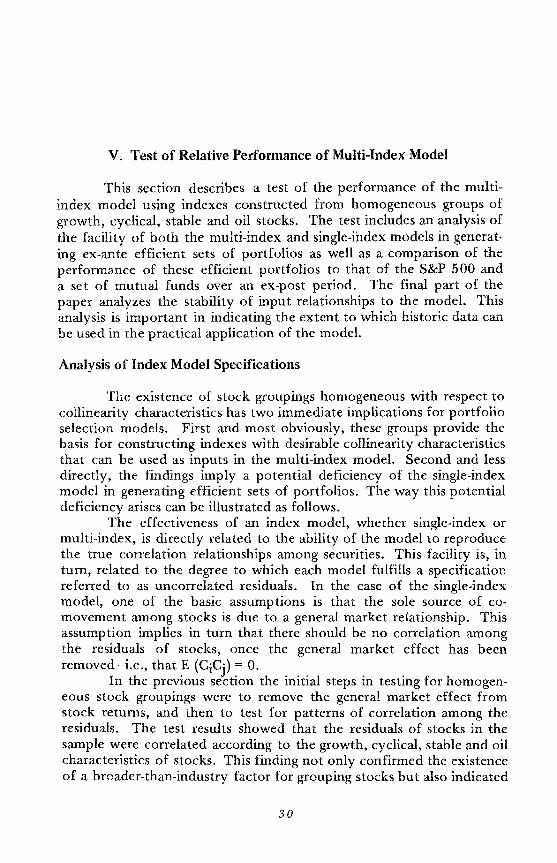
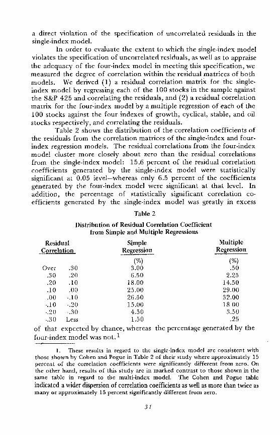
Table 2 shows the distribution of the correlation coefficients ofthe residuals from the correlation matrices of the single-index and four­index regression models. The residual correlations from the four-indexmodel duster more closely about zero than the residual correlationsfrom the single-index model: 15.6 percent of the residual correlationcoefficients generated by the single-index model were statisticallysignificant at 0.05 level-whereas only 6.5 percent of the coefficientsgenerated by the four-index model were significant at that level. Inaddition, the percentage of statistically significant correlation co­efficients generated by the single-index model was greatly in excess

Table 2

MultipleRegression

(%).50

2.2514.5029.0032.0018.00

3.50.25

the percentage generated by the

Distribution of Residual Correlation Coefficientfrom Simple and Multiple Regressions

SimpleRegression

ResidualCorrelation

(%)Over .30 3.00

.30 .20 6.50

.20 .10 18.00

.10 .00 25.00

.00 -.10 26.50-.10 -.20 15.00-.20 -.30 4.50-.30 Less 1.50

of that expected by chance, whereasfour-index model was not. 1

1. These results in regard to the single-index model are consistent withthose shown by Cohen and Pogue in Table 2 of their study where approximately 15percent of the correlation coefficients were significantly different from zero. Onthe other hand, results of this study are in marked contrast to those shown in thesame table in regard to the multi-index model. The Cohen and Pogue table

indicated a wider dispersion of correlation coefficients as well as more than twice asmany or approximately 15 percent significantly different from zero.

31

The extraordinary degree of correlation among the residualsfrom the single-index model provides further evidence that the speci­fication of uncorrelated residuals for this model is seriously violated.This violation results from the single-index model's failure to incorpor­ate systematic effects among securities other than those due to a com­mon relationship with a general market factor. As a result, it is likelythat the relationship among securities specified by the single-indexmodel will differ substantially from the true correlation relationships.

In contrast, the residuals in the four-index model are virtuallyuncorrelated. This model was more effective than the single-indexmodel in incorporating the major systematic elements explaining thecross-sectional structure of security returns over the 1961-69 periodof analysis. The relationship among securities implied by the four­index model more closely approximates the true correlation matrixthan that implied by the single-index model.

Ex-Ante Correlation Matrices

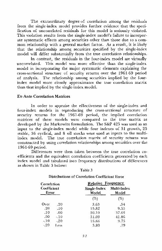
In order to appraise the effectiveness of the single-index andfour-index models in reproducing the cross-sectional structure ofsecurity returns for the 1961-69 period, the implied correlationmatrices of these models were compared to the true matrix asdeveloped by the Markowitz formulation. The S&P 425 was used as aninput to the single-index model while four indexes of 31 growth, 25stable, 36 cyclical, and 8 oil stocks were used as inputs to the multi­index model. The true correlation matrix of security returns wasconstructed by using correlation relationships among securities over the1961-69 period.

Differences were then taken between the true correlation co­efficients and the equivalent correlation coefficients generated by eachindex model and tabulated into frequency distributions of differencesas shown in Table 3 below:

Table 3

Distributions of Correlation Coefficient Error

CorrelationCoefficient

Error

Relative FrequencySingle-Index Multi-Index

Model Model

Over.20.10.00

-.10-.20

.20

.10

.00-.10-.20Less

32

(%)

3.6315.8230.1031.0915.66

3.80

(%)

.549.35

37.6941.86

9.75.79

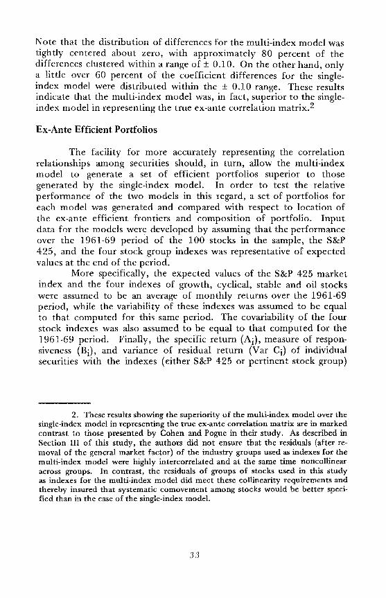
Note that the distribution of differences for the multi-index model wastightly centered about zero, with approximately 80 percent of thedifferences clustered within a range of ± 0.10. On the other hand, onlya little over 60 percent of the coefficient differences for the single­index model were distributed within the ± 0.10 range. These resultsindicate that the multi-index model was, in fact, superior to the single-index model in representing the true ex-ante correlation matrix.2 -

Ex-Ante Efficient Portfolios

The facility for more accurately representing the correlationrelationships among securities should, in turn, allow the multi-indexmodel to generate a set of efficient portfolios superior to thosegenerated by the single-index model. In order to test the relativeperformance of the two models in this regard, a set of portfolios foreach model was generated and compared with respect to location ofthe ex-ante efficient frontiers and composition of portfolio. Inputdata for the models were developed by assuming that the performanceover the 1961-69 period of the 100 stocks in the sample, the S&P425, and the four stock group indexes was representative of expectedvalues at the end of the period.

More specifically, the expected values of the S&P 425 marketindex and the four indexes of growth, cyclical, stable and oil stockswere assumed to be an average of monthly returns over the 1961-69period, while the variability of these indexes was assumed to be equalto that computed for this same period. The covariability of the fourstock indexes was also assumed to be equal to that computed for the1961-69 period. Finally, the specific return (Ai), measure of respon­siveness (Bi), and variance of residual return (Var Ci) of individualsecurities with the indexes (either S&P 425 or pertinent stock group)

2. These results showing the superiority of the multi-index model over thesingle-index model in representing the true ex-ante correlation matrix are in markedcontrast to those presented by Cohen and Pogue in their study. As described inSection III of this study, the authors did not ensure that the residuals (after re­moval of the general market factor) of the industry groups used as indexes for themulti-index model were highly intercorrelated and at the same time noncollinearacross groups. In contrast, the residuals of groups of stocks used in this studyas indexes for the multi-index model did meet these collinearity requirements andthereby insured that systematic comovement among stocks would be better speci­fied than in the case of the single-index model.

33

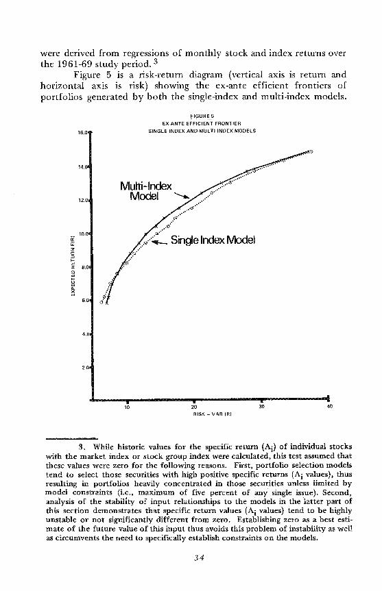
were derived from regressions of monthly stock and index returns overthe 1961-69 study period. 3

Figure 5 is a risk-return diagram (vertical axis is return andhorizontal axis is risk) showing the ex-ante efficient frontiers ofportfolios generated by both the single-index and multi-index models.

16.0

Fl.c;ll-f1E_5EX·ANTE EFFICIENT FRONTIER

SINGLE·INDEX AND MULTI·INDEX MODELS

Multi-Index w...·····,,············

Model ::<'! .e<

G.····.:/..",...~ Single Index Model

? .....'

{~.'

12.0

14.0

10.0ii:u:;za::::J...LUa: 8.00LU...~Q.

~6.0

4.0

2.0

10 20

RISK - VAR (RI

30 40

3. While historic values for the specific return (Ai) of individual stockswith the market index or stock group index were calculated, this test assumed thatthese values were zero for the following reasons. First, portfolio selection modelstend to select those securities with high positive specific returns (Ai values), thusresulting in portfolios heavily concentrated in those securities unless limited bymodel constraints (Le., maximum of five percent of any single issue). Second,analysis of the stability of input relationships to the models in the latter part ofthis section demonstrates that specific return values (Ai values) tend to be highlyunstable or not significantly different from zero. Establishing zero as a best esti­mate of the future value of this input thus avoids this problem of instability as wellas circumvents the need to specifically establish constraints on the models.

34

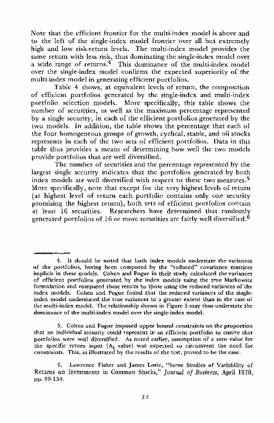
Note that the efficient frontier for the multi-index model is above andto the left of the single-index model frontier over all but extremelyhigh and low risk-return levels. The multi-index model provides thesame return with less risk, thus dominating the single-index model overa wide range of returns.4 This dominance of the multi-index modelover the single-index model confirms the expected superiority of themulti-index model in generating efficient portfolios.

Table 4 shows, at equivalent levels of return, the compositionof efficient portfolios generated by the single-index and multi-indexportfolio selection models. More specifically, this table shows thenumber of securities, as well as the maximum percentage representedby a single security, in each of the efficient portfolios generated by thetwo models. In addition, the table shows the percentage that each ofthe four homogeneous groups of growth, cyclical, stable, and oil stocksrepresents in each of the two sets of efficient portfolios. Data in thistable thus provides a means of determining how well the two modelsprovide portfolios that are well diversified.

The number of securities and the percentage represented by thelargest single security indicates that the portfolios generated by bothindex models are well diversified with respect to these two measures.5

More specifically, note that except for the very highest levels of return(at highest level of return each portfolio contains only one securitypromising the highest return), both sets of efficient portfolios containat least 16 securities. Researchers have determined that randomlygenerated portfolios of 16 or more securities are fairly well diversified.6

4. It should be noted that both index models understate the variancesof the portfolios, having been computed by the "reduced" covariance matricesimplicit in these models. Cohen and Pogue in their study calculated the variancesof efficient portfolios generated by the index models using the true Markowitzformulation and compared these results 'to tpose using the reduced variances of theindex models. Cohen and Pogue found that the reduced variances of the single­index model understated the true variances to a greater extent than in the case ofthe multi-index model. The relationship shown in Figure 5 may thus understate thedominance of the multi-index model over the single-index model.

5. Cohen and Pogue imposed upper bound constraints on the proportionthat an individual security could represent in an efficient portfolio to ensure thatportfolios were well diversified. As noted earlier, assumption of a zero value forthe specific return input (Ai value) was expected to circumvent the need forconstraints. This, as illustrated by the results of the test, proved to be the case.

6. Lawrence Fisher and James Lorie, "Some Studies of Variability ofReturns on Investments in Common Stocks," Journal of Business, April 1970,pp.99-134.

35

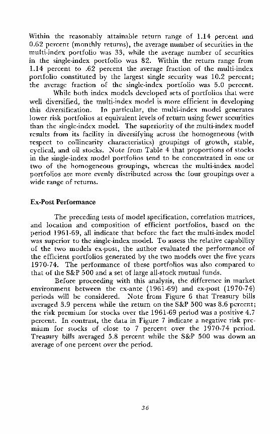
Within the reasonably attainable return range of 1.14 percent and0.62 percent (monthly returns), the average number of securities in themulti-index portfolio was 33, while the average number of securitiesin the single-index portfolio was 82. Within the return range from1.14 percent to .62 percent the average fraction of the multi-indexportfolio constituted by the largest single security was 10.2 percent;the average fraction of the single-index portfolio was 5.0 percent.

While both index models developed sets of portfolios that werewell diversified, the multi-index model is more efficient in developingthis diversification. In particular, the multi-index model generateslower risk portfolios at equivalent levels of return using fewer securitiesthan the single-index model. The superiority of the multi-index modelresults from its facility in diversifying across the homogeneous (withrespect to collinearity characteristics) groupings of growth, stable,cyclical, and oil stocks. Note from Table 4 that proportions of stocksin the single-index model portfolios tend to be concentrated in one ortwo of the homogeneous groupings, whereas the multi-index modelportfolios are more evenly distributed across the four groupings over awide range of returns.

Ex-Post Perfonnance

The preceding tests of model specification, correlation matrices,and location and composition of efficient portfolios, based on theperiod 1961-69, all indicate that before the fact the multi-index modelwas superior to the single-index model. To assess the relative capabilityof the two models ex-post, the author evaluated the performance ofthe efficient portfolios generated by the two models over the five years1970-74. The performance of these portfolios was also compared tothat of the S&P 500 and a set of large all-stock mutual funds.

Before proceeding with this analysis, the difference in marketenvironment between the ex-ante (1961-69) and ex-post (1970-74)periods will be considered. Note from Figure 6 that Treasury billsaveraged 3.9 percent while the return on the S&P 500 was 8.6 percent;the risk premium for stocks over the 1961-69 period was a positive 4.7percent. In contrast, the data in Figure 7 indicate a negative risk pre­mium for stocks of close to 7 percent over the 1970-74 period.Treasury bills averaged 5.8 percent while the S&P 500 was down anaverage of one percent over the period.

36

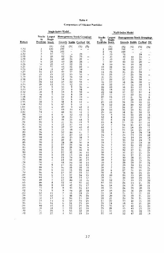
Table 4

Composition of Efficient Portfolios

Single Index Model Multi-Index Model

Stocks Largest Homogeneous Stock Groupings Stocks Largest Homogeneous Stock GroupinBsin Single 10 Single

Return ~Stock ~ Stable Cyclical 2!'.. Portfolio Stock Growth Stable Cyclical .2!!...-----('Yo) ('Yo) ('Yo) ('Yo) ('Yo) ('Yo) ('Yo) ('Yo) ('Yo) (%)

1.34 I 100 100 I 100 1001.33 2 76 100 2 91 1001.32 3 47 77 23 3 53 76 241.29 5 25 52 25 23 4 33 ,12 33 251.28 6 26 49 26 25 5 33 41 33 261.27 8 25 49 25 26 7 32 39 32 291.25 10 22 47 22 31 8 30 34 30 361.2'1 11 21 46 21 33 10 29 34 29 371.23 14 19 ·17 19 34 13 27 36 27 371.22 Hi 17 ·19 17 34 14 26 36 26 381.20 19 15 52 15 33 15 25 37 25 381.19 21 14 53 14 39. 16 24 37 24 39.,1.18 24 13 54 13 33 17 23 37 24 391.1 7 26 12 53 12 35 18 22 38 24 381.16 28 12 53 12 35 19 22 37 24 38 1Ll4 33 9 55 9 36 20 19 36 23 37 4!.I 3 3·1 9 53 9 38 22 18 37 22 37 4Ll2 36 8 54 8 38 22 18 37 22 37 ·1!.II 38 7 53 8 39 22 17 37 22 36 51.08 46 6 52 8 40 22 15 37 21 34 81.06 51 5 52 8 40 21 14 37 20 33 101.05 £:18 5 48 8 H 23 13 36 20 33 II1.04 59 5 47 9 H 24 12 36 20 32 121.03 61 4 49 <) 41 I 27 II 36 21 'II 121.01 70 4 44 10 45 I 28 10 36 20 31 131.00 74 4 44 II 44 I 29 10 36 21 30 13

.98 77 4 'II 12 45 2 30 9 35 22 29 14

.96 82 3 39 14 44 3 32 8 35 22 28 15.95 87 3 38 15 44 3 .12 8 35 23 27 15.94 90 3 37 16 44 3 33 8 34 23 27 169" 91 3 35 17 44 4 33 7 34 23 27 16• J

.91 95 3 32 17 45 6 32 7 34 24 25 17

.90 96 3 31 18 45 6 32 34 24 25 17

.89 98 3 32 20 '11 33 34 24 24 18

.88 99 3 31 22 40 34 3,1 24 2·1 18

.87 99 3 30 25 38 3'1 34 24 24 18

.86 99 2 29 27 37 7 34 33 24 2-l 19

.85 99 2 28 28 36 8 35 33 25 23 19

.84 99 2 27 29 36 8 36 33 26 22 19

.83 99 2 26 29 36 9 36 32 27 21 20

.81 99 2 24 31 36 9 39 32 27 21 21

.80 99 3 22 32 36 10 39 31 27 21 21

.79 99 3 20 34 36 10 39 31 27 21 21

.78 99 4 19 34 36 11 39 30 28 21 21:i7 99 4 18 35 35 12 39 30 28 21 21.76 99 4 18 :H 35 13 39 29 29 21 21.74 99 17 35 35 13 38 29 29 21 21.73 99 5 16 35 35 14 38 28 30 21 21.71 99 5 16 35 35 14 38 8 27 31 21 21.70 96 6 15 37 33 15 39 8 26 32 21 21.69 95 6 14 37 34 15 39 10 26 33 20 21.68 94 7 13 39 33 15 38 11 26 3:3 20 21.66 89 7 12 40 :l2 16 38 12 24 33 23 20.65 86 8 12 41 31 16 37 13 24 34 21 21.64 80 8 10 42 'II 17 36 14 24 35 20 216" 75 9 9 43 31 17 35 15 24 35 20 21..,

.62 71 9 9 44 29 18 33 16 24 36 20 20

.60 63 II 46 28 19 31 18 21 37 21 21

.59 57 12 48 25 20 28 20 20 39 21 20

.58 55 H 6 50 24 20 28 21 20 39 21 20

.57 53 14 6 50 24 20 27 22 19 'lO 21 20

.55 47 16 6 51 23 20 26 2-l 18 'll 21 20

.54 ·10 16 5 52 23 20 25 25 17 42 21 20

.52 38 18 53 22 20 25 28 15 43 22 20

.-4-9 31 25 4 55 22 19 24 31 13 ·16 22 19048 25 27 ·1 54 23 19 22 33 12 47 22 19

37

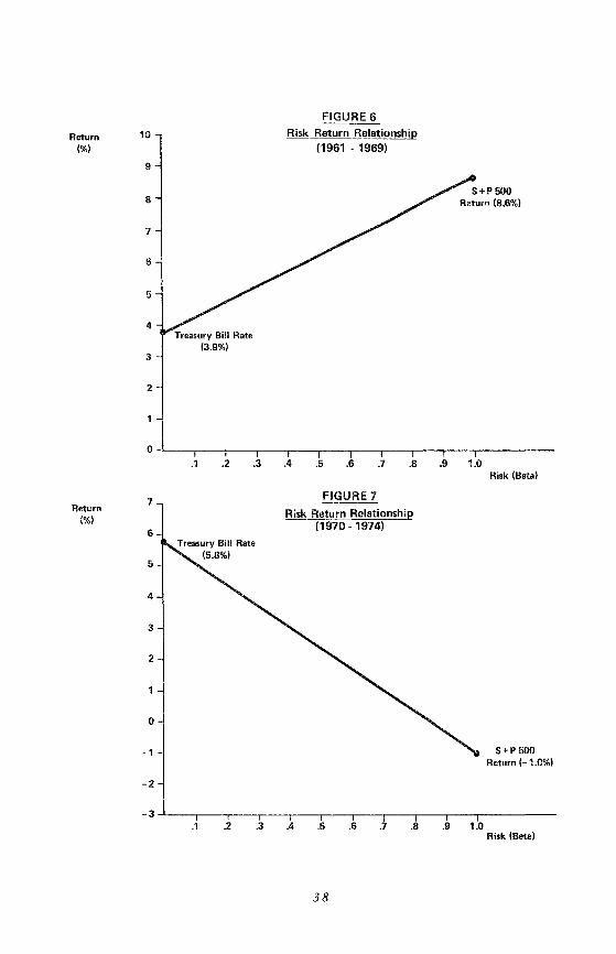
Return(%)

10

9

8

7

6

5

4

3

2

Treasury Biii Rate(3.9%)

FIGURE 6

Risk Return Relationship(1961 - 1969)

.1 .2 .3 .4 .5 .6 .7 .8 .9 1.0Risk (Beta)

Return(%)

7

6

5

4

3

2

o

- 1

-2

FIGURE 7

Risk Return Relationship(1970 - 1974)

S+P500Return (-1.0%)

-3 -<--,--,---,---,---,---,---,------.--.---.------.1 .2 .3 .4 .5

38

.6 .7 .8 .9 1.0Risk (Beta)

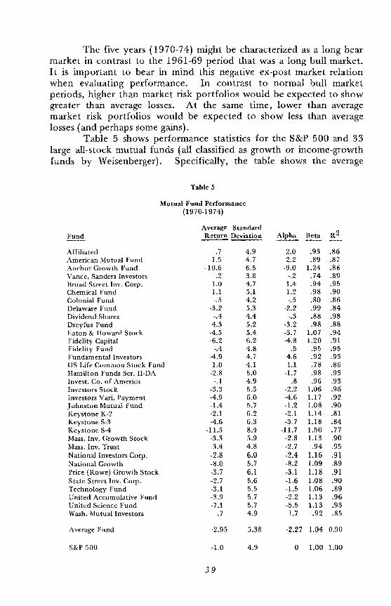
The five years (1970-74) might be characterized as a long bearmarket in contrast to the 1961-69 period that was a long bull market.It is important to bear in mind this negative ex-post market relationwhen evaluating performance. In contrast to normal bull marketperiods, higher than market risk portfolios would be expected to showgreater than average losses. At the same time, lower than averagemarket risk portfolios would be expected to show less than averagelosses (and perhaps some gains).

Table 5 shows performance statistics for the S&P 500 and 33large all-stock mutual funds (all classified as growth or income-growthfunds by Weisenberger). Specifically, the table shows the average

Table 5

Mutual Fund Performance(1970-1974)

Average StandardFund ~Deviation Alpha Beta R2

Affiliated .7 4.9 2.0 .93 .86American Mutual Fund 1.5 4.7 2.2 .89 .87Anchor Growth Fund -10.6 6.5 -9.0 1.24 .88Vance, Sanders Investors .2 3.8 -.2 .74 .89Broad Street Inv. Corp. 1.0 4.7 1.4 .94 .95Chemical Fund 1.1 5.1 1.2 .98 .90Colonial Fund -.5 4.2 -.5 .80 .86Delaware Fund -3.2 5.3 -2.2 .99 .84Dividend Shares -.4 4.4 -.3 .88 .98Dreyfus Fund -4.3 5.2 -3.2 .98 .88Eaton & Howard Stock -4.5 5.4 -3.7 1.07 .94Fidelity Capital -6.2 6.2 -4.8 1.20 .91Fidelity Fund -.4 4.8 .5 .95 .95Fundamental Investors -4.9 4.7 -4.6 .92 .93US Life Common Stock Fund 1.0 4.1 1.1 .78 .86Hamilton Funds Ser. H-DA -2.8 5.0 -1. 7 .98 .93Invest. Co. of America -.1 4.9 .8 .96 .93Investors Stock -3.3 5.3 -2.2 1.06 .96Investors Vari. Payment -4.9 6.0 -4.6 1.17 .92Johnston Mutual Fund -1.4 5.7 -1.2 1.08 .90Keystone K-2 -2.1 6.2 -2.1 1.14 .81Keystone S-3 -4.6 6.3 -3.7 1.18 .84Keystone S-4 -11.5 8.4 -11.7 1.50 .77Mass. Inv. Growth Stock -3.3 5.9 -2.8 1.13 .90Mass. Inv. Trust -3.4 4.8 -2.7 .94 .95National Investors Corp. -2.8 6.0 -2.4 1.16 .91National Growth -8.0 5.7 -8.2 1.09 .89Price (Rowe) Growth Stock -3.7 6.1 -3.1 1.18 .91State Street Inv. Corp. -2.7 5.6 -1.6 1.08 .90Technology Fund -3.1 5.5 -1.5 1.06 .89United Accumulative Fund -3.9 5.7 -2.2 1.13 .96United Science Fund -7.1 5.7 -5.5 1.13 .93Wash. Mutual Investors .7 4.9 1.7 .92 .85

Average Fund -2.95 5.38 -2.27 1.04 0.90

S&P 500 -1.0 4.9 0 1.00 1.00

39

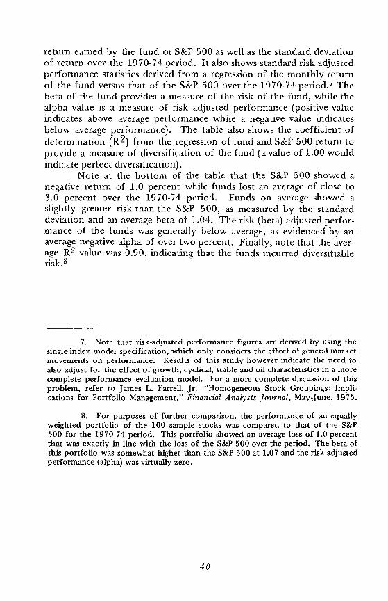
return earned by the fund or S&P 500 as well as the standard deviationof return over the 1970-74 period. It also shows standard risk adjustedperformance statistics derived from a regression of the monthly returnof the fund versus that of the S&P 500 over the 1970-74 period.7 Thebeta of the fund provides a measure of the risk of the fund, while thealpha value is a measure of risk adjusted performance (positive valueindicates above average performance while a negative value indicatesbelow average performance). The table also shows the coefficient ofdetermination (R2) from the regression of fund and S&P 500 return toprovide a measure of diversification of the fund (a value of 1.00 wouldindicate perfect diversification).

Note at the bottom of the table that the S&P 500 showed anegative return of 1.0 percent while funds lost an average of close to3.0 percent over the 1970-74 period. Funds on average showed aslightly greater risk than the S&P 500, as measured by the standarddeviation and an average beta of 1.04. The risk (beta) adjusted perfor­mance of the funds was generally below average, as evidenced by anaverage negative alpha of over two percent. Finally, note that the aver­age R2 value was 0.90, indicating that the funds incurred diversifiablerisk.8

7. Note that risk-adjusted performance figures are derived by using thesingle-index model specification, which only considers the effect of general marketmovements on performance. Results of this study however indicate the need toalso adjust for the effect of growth, cyclical, stable and oil characteristics in a morecomplete performance evaluation model. For a more complete discussion of thisproblem, refer to James L. Farrell, Jr., "Homogeneous Stock Groupings: Impli­cations for Portfolio Management," Financial Analysts Journal, May-June, 1975.

8. For purposes of further comparison, the performance of an equallyweighted portfolio of the 100 sample stocks was compared to that of the S&P500 for the 1970-74 period. This portfolio showed an average loss of 1.0 percentthat was exactly in line with the loss of the S&P 500 over the period. The beta ofthis portfolio was somewhat higher than the S&P 500 at 1.07 and the risk adjustedperformance (alpha) was virtually zero.

40

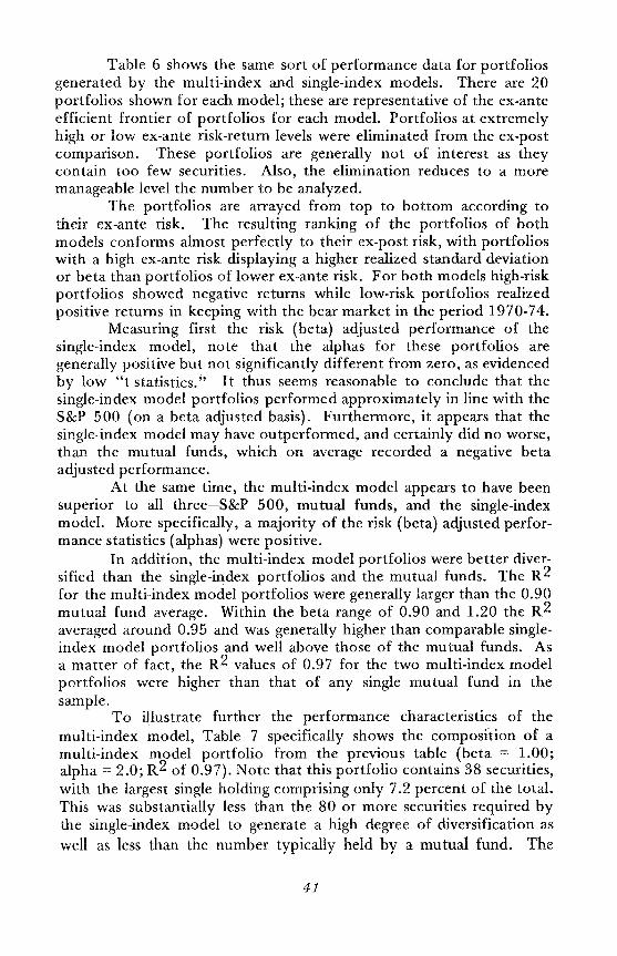
Table 6 shows the same sort of performance data for portfoliosgenerated by the multi-index and single-index models. There are 20portfolios shown for each model; these are representative of the ex-anteefficient frontier of portfolios for each model. Portfolios at extremelyhigh or low ex-ante risk-return levels were eliminated from the ex-postcomparison. These portfolios are generally not of interest as theycontain too few securities. Also, the elimination reduces to a moremanageable level the number to be analyzed.

The portfolios are arrayed from top to bottom according totheir ex-ante risk. The resulting ranking of the portfolios of bothmodels conforms almost perfectly to their ex-post risk, with portfolioswith a high ex-ante risk displaying a higher realized standard deviationor beta than portfolios of lower ex-ante risk. For both models high-riskportfolios showed negative returns while low-risk portfolios realizedpositive returns in keeping with the bear market in the period 1970-74.

Measuring first the risk (beta) adjusted performance of thesingle-index model, note that the alphas for these portfolios aregenerally positive but not significantly different from zero, as evidencedby low "t statistics.;' It thus seems reasonable to conclude that thesingle-index model portfolios performed approximately in line with theS&P 500 (on a beta adjusted basis). Furthermore, it appears that thesingle-index model may have outperformed, and certainly did no worse,than the mutual funds, which on average recorded a negative betaadjusted performance.

At the same time, the multi-index model appears to have beensuperior to all three-S&P 500, mutual funds, and the single-indexmodel. More specifically, a majority of the risk (beta) adjusted perfor­mance statistics (alphas) were positive.

In addition, the multi-index model portfolios were better diver­sified than the single-index portfolios and the mutual funds. The R2for the multi-index model portfolios were generally larger than the 0.90mutual fund average. Within the beta range of 0.90 and 1.20 the R2averaged around 0.95 and was generally higher than comparable single­index model portfolios and well above those of the mutual funds. Asa matter of fact, the R2 values of 0.97 for the two multi-index modelportfolios were higher than that of any single mutual fund In thesample.

To illustrate further the performance characteristics of themulti-index model, Table 7 specifically shows the composition of amulti-index model portfolio from the previous table (beta =: 1.00;alpha = 2.0; R2 of 0.97). Note that this portfolio contains 38 securities,with the largest single holding comprising only 7.2 percent of the total.This was substantially less than the 80 or more securities required bythe single-index model to generate a high degree of diversification aswell as less than the number typically held by a mutual fund. The

41

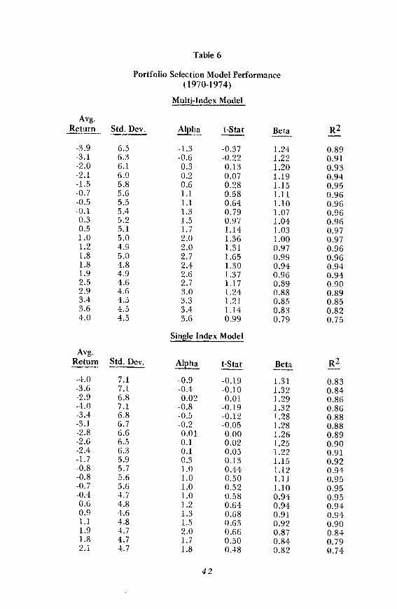
Table 6

Portfolio Selection Model Performance(1970-1974)

Multi-Index Model

Avg.R2Return Std. Dev. Alpha t-Stat Beta

-3.9 6.5 -1.3 -0.37 1.24 0.89-3.1 6.3 -0.6 -0.22 1.22 0.91-2.0 6.1 0.3 0.13 1.20 0.93-2.1 6.0 0.2 0.07 1.19 0.94-1.5 5.8 0.6 0.28 1.15 0.95-0.7 5.6 1.1 0.58 1.11 0.96-0.5 5.5 1.1 0.64 1.10 0.96-0.1 5.4 1.3 0.79 1.07 0.960.3 5.2 1.5 0.97 1.04 0.960.5 5.1 1.7 1.14 1.03 0.971.0 5.0 2.0 1.36 1.00 0.971.2 4.9 2.0 1.31 0.97 0.961.8 5.0 2.7 1.65 0.99 0.961.8 4.8 2.4 1.30 0.94 0.941.9 4.9 2.6 1.37 0.96 0.942.5 4.6 2.7 1.17 0.89 0.902.9 4.6 3.0 1.24 0.88 0.893.4 4.5 3.3 1.21 0.85 0.853.6 4.5 3.4 1.14 0.83 0.824.0 4.5 3.6 0.99 0.79 0.75

Single Index Model

Avg.R2Return Std. Dev. Alpha t-Stat Beta

-4.0 7.1 -0.9 -0.19 1.31 0.83-3.6 7.1 -0.4 -0.10 1.32 0.84-2.9 6.8 0.02 0.01 1.29 0.86-4.0 7.1 -0.8 -0.19 1.32 0.86-3.4 6.8 -0.5 -0.12 1.28 0.88-3.1 6.7 -0.2 -0.05 1.28 0.88-2.8 6.6 0.01 0.00 1.26 0.89-2.6 6.5 0.1 0.02 1.25 0.90-2.4 6.3 0.1 0.05 1.22 0.91-1. 7 5.9 0.3 0.13 1.15 0.92-0.8 5.7 1.0 0.44 1.12 0.94-0.8 5.6 1.0 0.50 1.11 0.95-0.7 5.6 1.0 0.52 1.10 0.95-0.4 4.7 1.0 0.58 0.94 0.950.6 4.8 1.2 0.64 0.94 0.940.9 4.6 1.3 0.68 0.91 0.941.1 4.8 1.5 0.63 0.92 0.901.9 4.7 2.0 0.66 0.87 0.841.8 4.7 1.7 0.50 0.84 0.792.1 4.7 1.8 0.48 0.82 0.74

42

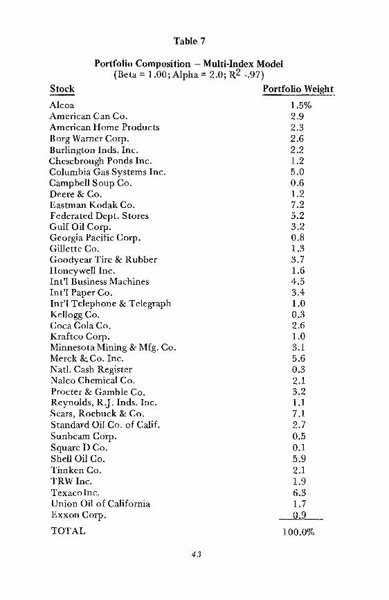
Table 7

Portfolio Composition - Multi-Index Model(Beta = 1.00; Alpha = 2.0; R2 -.97)

Portfolio Weight

1.5%2.92.32.62.21.25.00.61.27.25.23.20.81.33.71.64.53.41.00.32.61.03.15.60.32.13.21.17.12.70.50.15.92.11.96.31.70.9

Stock

AlcoaAmerican Can Co.American Home ProductsBorg Warner Corp.Burlington Inds. Inc.Chesebrough Ponds Inc.Columbia Gas Systems Inc.Campbell Soup Co.Deere & Co.Eastman Kodak Co.Federated Dept. StoresGulf Oil Corp.Georgia Pacific Corp.Gillette Co.Goodyear Tire & RubberHoneywell Inc.Int'l Business MachinesInt'l Paper Co.Int'l Telephone & TelegraphKellogg Co.Coca Cola Co.Kraftco Corp.Minnesota Mining & Mfg. Co.Merck &. Co. Inc.Nat!. Cash RegisterNalco Chemical Co.Procter & Gamble Co.Reynolds, R.J. Inds. Inc.Sears, Roebuck & Co.Standard Oil Co. of Calif.Sunbeam Corp.Square DCa.Shell Oil Co.Timken Co.TRW Inc.Texacolnc.Union Oil of CaliforniaExxon Corp.

TOTAL 100.0%

43

multi-index model thus achieves efficient diversification while demon­strating superior ex-post performance with a positive alpha of 2.0percent. In sum, it seems reasonable to conclude that the multi-indexmodel not only has superior ex-ante, but also superior ex-post proper­ties.

Test of Stability of Input Relationships

The final part of this section discusses the stability of inputrelationships to the multi-index model. This assessment is important,since the ease of practical implementation of the model depends onstability of the inputs over time. More specifically, the greater theirstability, the more extensively historic data may be used as inputs,thus avoiding recourse to developing inputs by more arbitrary or ex­pensive approaches. Recall that inputs required for the multi-indexmodel are estimates for the four indexes of growth, cyclical, stable, andoil stocks, as well as estimates of the values relating individual stocks ina group with their corresponding index.

The analysis began by assessing the stability over time of thecorrelation relationships among the four groupings of growth, cyclical,stable, and oil stocks. This stability can be assessed by means ofthe index procedure used in the previous section to measure the de­gree to which the four stock groupings showed characteristics of highwithin-group correlation and low between-group correlation.Previously applied to the 1961-69 period, this procedure involvedforming indexes from the stocks within each of the four groups andthen correlating individual stocks with each of the four indexes. Weapplied this procedure to the sample stock data for the 1970-74performance period and compared the results.

Figure 8 shows the results of the index procedure for the 1970­74 ex-post period (Figure 4 in the previous section shows the results forthe 1961-69 period). The two figures display summary matricesshowing the average value of the correlation coefficients of the stockswithin each group (growth, cyclical, stable, oil) with the correspondingindex, as well as with the other three indexes. Comparing the 1970-74results to those of the earlier 1961-69 period, one sees the same desir­able pattern of high within-group correlation, and low across-groupcorrelation. The average values of the correlation coefficients betweenstocks and the index to which assigned were all positive and highlysignificant. In contrast, stocks showed a low degree of correlation withindexes other than the one to which assigned. These results indicate afairly high degree of stability over time in the. relationship amonggroupmgs.

44

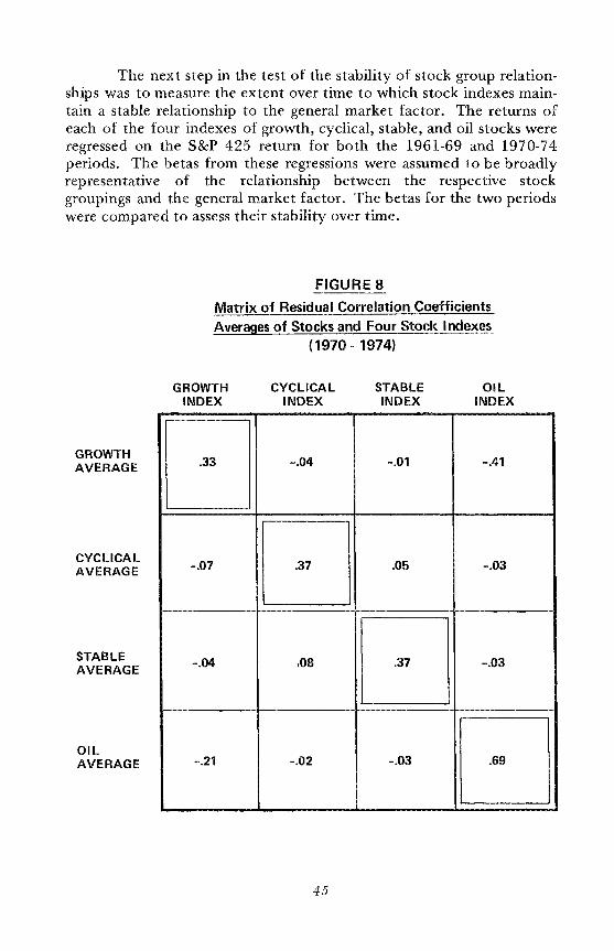
The next step in the test of the stability of stock group relation­ships was to measure the extent over time to which stock indexes main­tain a stable relationship to the general market factor. The returns ofeach of the four indexes of growth, cyclical, stable, and oil stocks wereregressed on the S&P 425 return for both the 1961-69 and 1970-74periods. The betas from these regressions were assumed to be broadlyrepresentative of the relationship between the respective stockgroupings and the general market factor. The betas for the two periodswere compared to assess their stability over time.

FIGURE 8

Matrix of Residual Correlation CoefficientsAverages of Stocks and Four Stock Indexl}~

(1970 - 1974)

GROWTHINDEX

CYCLICALINDEX

STABLEINDEX

OILINDEX

GROWTHAVERAGE

CYCLICALAVERAGE

STABLEAVERAGE

OILAVERAGE

[J -.04 -.01 -.41

-.07 D .05 -.03

-.04 ,08 D -.03

-.21 -.02 -.03 [J45

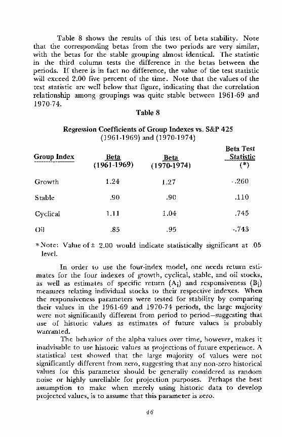
Table 8 shows the results of this test of beta stability. Notethat the corresponding betas from the two periods are very similar,with the betas for the stable grouping almost identical. The statisticin the third column tests the difference in the betas between theperiods. If there is in fact no difference, the value of the test statisticwill exceed 2.00 five percent of the time. Note that the values of thetest statistic are well below that figure, indicating that the correlationrelationship among groupings was quite stable between 1961-69 and1970-74.

Table 8

Regression Coefficients of Group Indexes vs. S&P 425(1961-1969) and (1970-1974)

Beta TestGroup Index Beta Beta Statistic

(1961-1969) (1910-1914) (*)

Growth 1.24 1.27 -.260

Stable .90 .90 .no

Cyclical 1.11 1.04 .745

Oil .85 .95 -.743

*- Note: Value of ± 2.00 would indicate statistically significant at .05level.

In order to use the four-index model, one needs return esti­mates for the four indexes of growth, cyclical, stable, and oil stocks,as well as estimates of specific return (Ai) and responsiveness (Bi)measures relating individual stocks to their respective indexes. Whenthe responsiveness parameters were tested for stability by comparingtheir values in the 1961-69 and 1970-74 periods, the large m~ority

were not significantly different from period to period-suggesting thatuse of historic values as estimates of future values is probablywarranted.

The behavior of the alpha values over time, however, makes itinadvisable to use historic values as projections of future experience. Astatistical test showed that the large majority of values were notsignificantly different from zero, suggesting that any non-zero historicalvalues for this parameter should be generally considered as randomnoise or highly unreliable for projection purposes. Perhaps the bestassumption to make when merely using historic data to developprojected values, is to assume that this parameter is zero.

46

VI. Summary and Conclusion

A pnme purpose of this study was to develop homogeneousstock groupings suitable for use as inputs in a multi-index model.Several statistical techniques were employed in testing whether theresiduals obtained by removing general market effects from a sample of100 stocks displayed the pattern of cross-sectional dependence thatwould conform to the hypothesized three stock categories. Thesestatistical procedures showed that the sample of 100 stocks could beclassified into four, rather than three, distinct groups, with an oilgroup being the unexpected fourth group. In addition, regression ana­lysis results indicated that, over the full period of the study, thesestock groupings accounted for an average of 15 percent of the variancein rate of return of stocks in the sample, over and above the 30 per­cent explained by the general market factor. This result suggested that,in addition to market and industry factors, a set of explanatory factorsbased on classification of stocks according to: (1) growth, (2) stable,(3) cyclical, and (4) oil would be useful in explaining the variation instock returns over time.

The existence of such stock groupings implies that residuals forthe single-index model are not uncorrelated. An examination of theresidual correlation matrix for this model confirmed the existence of asignificant degree of dependence among the residuals, whereas an exam­ination of this matrix for the four-index model showed very littledependence. The correlation matrix of stock returns implied by thefour-index model provides a closer approximation to the true correla­tion matrix than is provided by the single-index model, hence account­ing more satisfactorily for systematic effects among securities.

As a result, it was expected that portfolio selection based on themulti-index model would provide performance superior to selectionbased on the single-index model. Comparison of respective sets ofefficient portfolios generated by the two models showed that the multi­index model provided portfolios with lower risk at equivalent returnover a broad range of the efficient frontier. The multi-index modeldiversified more efficiently than the single-index model owing to thefacility for distributing the portfolio more evenly across the fourhomogeneous groups of growth, cyclical, stable, and oil stocks.

47

The relative performance of the two models was subjected toex-post test over the period 1970-74 using historical (1961-69) dataas inputs to the models. The performance of these models was alsocompared to that of large all-stock mutual funds and the S&P 500.Both models outperformed the mutual funds, with the single-indexmodel showing performance approximately in line with the S&P500 over the 1970-74 period. The multi-index model, by outperform­ing both the single-index model and the S&P 500, displayed not onlysuperior ex-ante, but also superior ex-post properties.

Finally, the study analyzed the stability of the parameters ofthe multi-index model. Tests indicated that, between the 1961-69and 1970-74 periods, the growth, cyclical, stable, and oil groups main­tained stable values for the relationships between individual stocksand their corresponding indexes. This stability suggests the pos­sibility of extensive use of historic values as inputs, thereby avoidingrecourse to more expensive or arbitrary approaches.

In conclusion, analysis of the characteristics of the multi-indexportfolio selection model indicates that it has significant potentialadvantage over other types of portfolio selection models. It alsoappears to have a potential advantage over traditional practical port­folio management practice, as evidenced by the superiority of itsperformance to that of mutual funds. Finally, the stability of some ofthe input relationships indicates that the process of practical imple­mentation may be easier than might be expected. The multi-indexmodel should in fact be the preferred model for practical portfolioanalysis.

48