Paper presented at the Learning Progressions in Science (LeaPS) Conference, June 2009, Iowa City, IA

THE PSYCHOMETRIC MODELING OF ORDERED MULTIPLE-CHOICE ITEM RESPONSES FOR DIAGNOSTIC ASSESSMENT WITH A LEARNING PROGRESSION

This paper focuses on the psychometric modeling of a specific item format known as ordered multiple choice (OMC). The OMC item format was developed to facilitate diagnostic assessment on the basis of levels from an underlying learning progression that is linked to constrained item response options. Though OMC items were developed by following the building blocks of BEAR Assessment System (BAS) developed by Mark Wilson and colleagues, it is shown that these items have features that seem to make them a poor match with the Rasch-based modeling approach typically taken in BAS applications. Some questions are raised about the use of Wright Maps, a key element of the BAS, to facilitate diagnostic classifications. An alternative modeling strategy is proposed, based on a recent extension to Tatsuoka’s Rule Space Method known as the Attribute Hierarchy Method (AHM; Leighton, Gierl, & Hunka, 2004). While the AHM has not previously been applied in the context of learning progression assessments with OMC items, it has some promising features that are illustrated at some length.

Derek C. Briggs, University of Colorado Alicia C. Alonzo, University of Iowa

Introduction

Learning progressions are becoming increasingly popular in science education. One of the more appealing features of learning progressions is their potential use to facilitate diagnostic assessments of student understanding. Diagnostic assessment hinges upon the development of items (i.e., tasks, problems) that can be used to efficiently elicit student conceptions such that these conceptions can be related back to a hypothesized learning progression. Briggs et al (2006) introduced Ordered Multiple-Choice (OMC) items as a means to this end. OMC items represent an attempt to combine the efficiency of traditional multiple choice items with the qualitative richness of the responses to open-ended questions. The potential efficiency comes from the fact that OMC items feature a constrained set of response options that can be scored objectively; the potential qualitative richness comes from the fact that each OMC response option has been designed to correspond to what students might answer in response to an open-ended question, and these answers have been explicitly linked to a discrete level on an underlying learning progression. The OMC item format belongs to a broader class of constrained assessment items in which the interest is not solely on whether a student has chosen the “scientifically correct” answer, but on diagnosing the reasons behind a student’s choice of a less scientifically correct answer (c.f., Minstrell, n.d.; 1992; 2000). An appealing aspect of such items is that they are consistent with the spirit behind learning progressions, which at root represent an attempt to classify the gray area of cognition that muddies the notion that students either “get something” or they “don’t.”

2

The focus of this paper is on the psychometric modeling of OMC item responses. More specifically, our interest is in conceptualizing an appropriate method by which a pattern of OMC item responses can be used to provisionally classify a student at a distinct location of a learning progression. There are two reasons why formal modeling is central to the burgeoning interest in learning progressions. First, item response modeling makes it possible to draw probabilistic inferences about unobserved (i.e., latent) states of student understanding. Second, and perhaps most importantly, the process of specifying a model and evaluating its fit provides a systematic means of validating and refining a hypothesized learning progression. Whether a learning progression is a basis for formal or informal diagnostic assessment at a local (i.e., classroom) or large-scale (i.e., state or federal) level, the choice of an associated psychometric model—or failure to take this choice seriously—will be consequential. A poorly chosen model might mask problems with assessment items, the underlying learning progression, or both. In contrast, a carefully chosen model will bring such problems to the surface for closer inspection. There are four sections that follow. In the first we provide a brief background on the development of a specific learning progression and associated set of OMC items around conceptual understanding of Earth and the Solar System. In the second section we present descriptive statistics from a recent administration of these OMC items to a convenience sample of over 1,088 high school students in Iowa. In the third section we discuss aspects of these OMC items that make them difficult to model using extensions of the Rasch Model, an approach that is common for assessment modeling in science education (Kennedy & Wilson, 2008; Liu & Boone, 2006). In the fourth section we introduce the Attribute Hierarchy Method (AHM; Leighton, Gierl & Hunka, 2004). The AHM builds upon the seminal work of Tatsuoka who developed what is known as the Rule Space Method for cognitive assessment (Tatsuoka, 1983; 2009). To our knowledge neither the AHM or Tatsuoka’s Rule Space Method has ever been applied in the context of a learning progression in the domain of science. We explore the transformations that would be necessary to apply the AHM to OMC item responses.

Background In previous studies we have developed learning progressions in the science content domains of earth science, life science and physical science (Alonzo & Steedle, 2009; Briggs, Alonzo, Schwab, & Wilson, 2006). We use a learning progression that focuses on conceptual understanding about Earth in the Solar System (ESS) as the context for the modeling issues that follow. The ESS learning progression describes students’ developing understanding of a target idea in earth science which, according to national science education standards documents, they should master by the end of 8th grade. However, there is substantial evidence (e.g., Halloun & Hestenes, 1985; Schneps & Sadler, 1987; Trumper & Gorsky, 1996) that typical instruction has not been successful in helping students to achieve these levels of understanding. In fact, many college students retain misconceptions about these target ideas. We began by defining a change along a single construct as our learning progression of interest. As the targeted knowledge whose development is described by the learning progression, the construct can also be considered to define the top level of the learning progression. We relied upon national science education documents (American Association for the Advancement of

3

Science [AAAS], 1993; NRC, 1996) for these definitions. With respect to ESS, by the end of 8th grade, students are expected to use an understanding of the relative motion of the Earth and other objects in the Solar System to explain phenomena such as the day/night cycle, the phases of the Moon, and the seasons. Lower levels of the learning progressions (i.e., novice understanding, intermediate understanding, etc.) were defined using research literature on students’ understanding of the targeted concepts (Atwood & Atwood, 1996; Baxter, 1995; Bisard, Aron, Francek, & Nelson, 1994; Dickinson, Flick, & Lederman, 2000; Furuness & Cohen, 1989; Jones, Lynch, & Reesink, 1987; Kikas, 1998; Klein, 1982; Newman, Morrison, & Torzs, 1993; Roald & Mikalsen, 2001; Sadler, 1987, 1988; Samarapungavan, Vosniadou, & Brewer, 1996; Stahly, Krockover, & Shepardson, 1999; Summers & Mant, 1995; Targan, 1987; Trumper, 2001; Vosniadou, 1991; Vosniadou & Brewer, 1994; Zeilik, Schau, & Mattern, 1998). In defining the levels, we relied upon information about both “misconceptions” and productive – but naïve – ideas which could provide a basis for further learning. At this point, it is important to note two key limitations of the available research base for the construction of this (and most other) learning progressions. Although learning progressions aim to describe how understanding develops in a given domain, the available research evidence is primarily cross-sectional. So while we have important information about the prevalence of particular ideas at different ages, there has been little documentation of students actually progressing through these ideas. Each learning progression lays out one possible pathway that students might take in moving from their initial ideas to full understanding of the construct. Additional pathways likely exist but will only be uncovered with longitudinal accounts of student learning. In addition, much of the work in the area of ESS occurred in the context of an interest in students’ misconceptions in the 1980’s; therefore, research has tended to focus upon isolated ideas, rather than exploring the relationship between students’ ideas in a given domain. Since the construct for the ESS learning progressions encompasses multiple phenomena – the earth orbiting the sun, the earth rotating on its axis, and moon orbiting the earth –the definition of levels included grouping ideas about these phenomena on the basis of both experience and logical reasoning from experts. Thus, the learning progression represents a hypothesis – both about the ways in which students actually progress through identified ideas and about the ways in which ideas about different phenomena “hang together” as students move towards the targeted level of understanding. This hypothesis must be tested with further evidence, such that the development of a learning progression and its associated assessment items is an iterative process – the learning progression informs the development of assessment items, the items are used to collect data about student thinking, his data is linked back the initial progression through the use of a psychometric model, and this leads to revisions in both the items and the learning progression itself. The current version of the ESS learning progression is depicted in Figure 1. Within the science education community, there is currently great interest in learning progressions which not only specify different levels of student knowledge, but also include the way(s) in which students can be expected to demonstrate that knowledge (for example, through assessment tasks). Smith, Wiser, Anderson, & Krajcik (2006) have called for learning progressions to include “learning performances” (p. 9). In the ESS learning progression, such learning performances are implied: students are expected to use the targeted knowledge to explain or predict phenomena. These

4

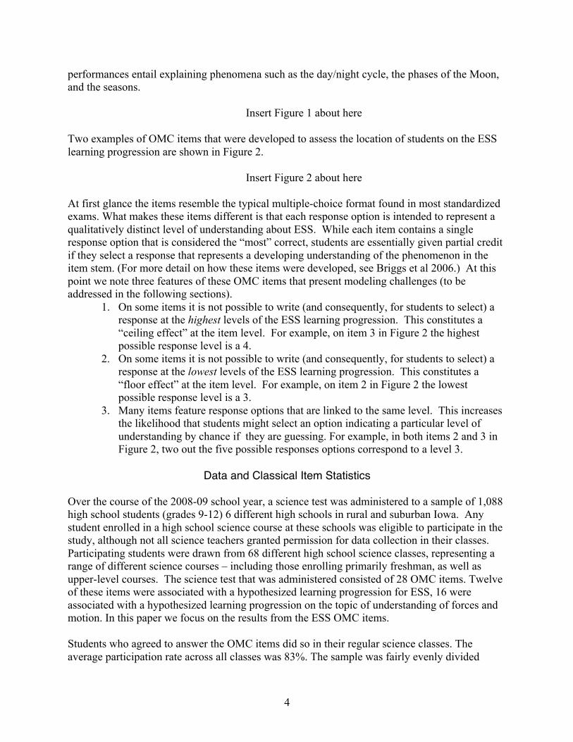
performances entail explaining phenomena such as the day/night cycle, the phases of the Moon, and the seasons.

Insert Figure 1 about here Two examples of OMC items that were developed to assess the location of students on the ESS learning progression are shown in Figure 2.

Insert Figure 2 about here At first glance the items resemble the typical multiple-choice format found in most standardized exams. What makes these items different is that each response option is intended to represent a qualitatively distinct level of understanding about ESS. While each item contains a single response option that is considered the “most” correct, students are essentially given partial credit if they select a response that represents a developing understanding of the phenomenon in the item stem. (For more detail on how these items were developed, see Briggs et al 2006.) At this point we note three features of these OMC items that present modeling challenges (to be addressed in the following sections).

1. On some items it is not possible to write (and consequently, for students to select) a response at the highest levels of the ESS learning progression. This constitutes a “ceiling effect” at the item level. For example, on item 3 in Figure 2 the highest possible response level is a 4.

2. On some items it is not possible to write (and consequently, for students to select) a response at the lowest levels of the ESS learning progression. This constitutes a “floor effect” at the item level. For example, on item 2 in Figure 2 the lowest possible response level is a 3.

3. Many items feature response options that are linked to the same level. This increases the likelihood that students might select an option indicating a particular level of understanding by chance if they are guessing. For example, in both items 2 and 3 in Figure 2, two out the five possible responses options correspond to a level 3.

Data and Classical Item Statistics

Over the course of the 2008-09 school year, a science test was administered to a sample of 1,088 high school students (grades 9-12) 6 different high schools in rural and suburban Iowa. Any student enrolled in a high school science course at these schools was eligible to participate in the study, although not all science teachers granted permission for data collection in their classes. Participating students were drawn from 68 different high school science classes, representing a range of different science courses – including those enrolling primarily freshman, as well as upper-level courses. The science test that was administered consisted of 28 OMC items. Twelve of these items were associated with a hypothesized learning progression for ESS, 16 were associated with a hypothesized learning progression on the topic of understanding of forces and motion. In this paper we focus on the results from the ESS OMC items. Students who agreed to answer the OMC items did so in their regular science classes. The average participation rate across all classes was 83%. The sample was fairly evenly divided

5

between male and female students (52% male; 48% female). High school students were chosen because the majority of these students could be expected to have been exposed to ideas relevant to the two learning progressions; this was thought to minimize guessing. After completing the ESS OMC items, students given a question which asked “Was the content of [these] questions covered in a science class you’ve taken?” While 46% of our sample responded “yes,” another 25% answered “no”, 28% answered “I am not sure” and 2% did not respond at all. Part of this can be explained by the fact that the timing of data collection was such that students were not currently studying topic related to ESS, even if this was part of the curriculum for their course, at the time of test administration.

Insert Figure 3 about here Figure 3 shows the distribution of student OMC item responses mapped back to the levels of the ESS progression. The items labeled in the columns of Figure 3 are arranged from easiest to hardest, where “easiness” is defined as the proportion of students selecting a response option at the highest possible level. So for example, 74% of students selected the highest possible response level for item 11 (“Which picture best represents the motion of the Earth (E) and Sun (S)?”), making it the easiest OMC item, while only 20% of students selected the highest possible response option for item 8 (“Which is the best explanation for why we see a full moon sometimes and a crescent moon other times?”), making it the hardest OMC item. The cells shaded gray represent levels for which there was no corresponding response option for the given OMC item. Note that there were only three items for which a response at the highest level of the ESS learning progression was possible, and on 5 out of 12 items, OMC responses were only linked to 3 out the 5 possible levels. Those cells with two numbers expressed as a sum represent items for which two options were associated with the same score level. For example, on item 11, roughly 7% of students chose response option A and 14% selected response option B, but both options are linked to level 2 of the ESS progression. Finally, the last row of Figure 3 provides the point-biserial associated with the highest level response option for each OMC item. Figure 3 conveys information that might be used to evaluate item quality. We see that a majority of students select responses in highest two levels of the ESS progression. In 5 out of 12 items, the proportion of students at each level decreases. Interestingly, all three items for which a response at level 5 was available had point-biserials less than 0.4—students selecting this option were not necessarily those who performed the best on the remaining items. Item 7 seems to stand out as a problematic item for two reasons: first, 61% of students chose responses at level 3 rather than at level 4 (29%); second, those students choosing level 4 seemed to have done so by chance because there is no significant correlation between a choice of level 4 and the total score on the remaining items (point-biserial = .12)1. Finally, without imposing any sort of item response model, one could use true score theory to estimate the reliability of the total scores deriving from these items. An estimate based on Cronbach’s alpha coefficient suggests a reliability of 0.67.

1 The stem for this item was “A solar eclipse is possible because” and the level 4 response option was “The Sun is much bigger than the Moon and much further away from the Earth.” The level 3 response chosen more frequently was “The Moon is always closer to the Earth than the Sun is.” While the former response is in fact more correct because it captures the key relationship between size and distance, one might also make the case that the latter response is also indicative of level 4 thinking.

6

There is certainly nothing “wrong” with the analysis above, which seems to suggest that some of the items from the test may need to be rewritten, or that the links between the options and ESS levels need to be reconsidered. However, these interpretations are somewhat arbitrary because, as is well-known, they are highly dependent on the particular sample of students taking the exam and the curriculum to which they have been exposed. If, for example, we were to find that the highest proportion of students were responding to options associated with levels 2 and 3, would this indicate a problem with the ordering of the item options, or could it reflect the fact that the students have not been exposed to this content in their curriculum? Furthermore, the analysis above does not provide any diagnostic assessment at the student level. Consider the following two randomly selected student response vectors “Liz”

Level 11 6 3 1 4 12 10 5 9 7 2 8 5 4 X X X X X X X X X X 3 X X 2 1

“Andrew”

Level 11 6 3 1 4 12 10 5 9 7 2 8 5 4 X X X X X X X 3 X X X X 2 1 X

While there appears to be considerable evidence to support the inference that Liz has an understanding of ESS at level 4, the pattern for Andrew is more ambiguous. We wish to choose a measurement model that allows probabilistic statements to be made about the ESS levels to which students such as Liz and Andrew can be appropriately classified. To meet this need in other contexts, Mark Wilson and colleagues have applied polytomous extensions of the Rasch Model to graphically place student ability and item difficulty on a common scale using what Wilson has termed a “Wright Map.” In the next section we explain why this approach does not seem appropriate for OMC items, as a motivation for our interest in an alternative modeling approach.

Some Problems with Wright Maps as a Tool for Diagnostic Classification

The work of Mark Wilson and colleagues on the development of systems of embedded assessments (e.g., the “BEAR Assessment System” (BAS)2) has been very influential and well-received in the science education research community. The BAS features four interrelated

2 For a detailed presentation of the principles and building blocks behind the BAS, see Wilson & Sloane, 2000 and Wilson, 2005.

7

“building blocks” that consist of (1) a construct map3, (2) an items design, (3) an outcome space, and (4) a measurement model. While building blocks 1-3 serve as the basis for the development and scoring of assessment items, it is the measurement model (building block 4) that serves to connect item responses back to the learning progression. The method by which this has been accomplished in all applications of the BAS with which we are aware is through the specification of a unidimensional or multidimensional Partial Credit Model (Masters, 1982; PCM) to place respondent ability and item difficulty on a common logit scale. The output from the PCM can be summarized graphically using a Wright Map. The Wright Map is then viewed as an empirical instantiation of a learning progression. To illustrate this, we consider an application of Wilson’s approach described in Kennedy & Wilson (2008). Briefly, the goal of the project was to use embedded assessments within a middle-school curriculum to facilitate the mapping of progress in student understanding of buoyancy over the course of a series of activities around the topic of “why things sink and float” (WTSF). To this end, a learning progression was developed to represent hypothesized levels of understanding for buoyancy, and the reasoning ability of students when they explained their answers. We focus attention just on the component of this learning progression related to understanding of buoyancy. In Figure 4 we recreate the buoyancy construct map (also known as a “progress variable”) from Kennedy & Wilson (2008), which distinguishes eight qualitatively and hierarchically distinct levels of student understanding.

Insert Figure 4 about here As a means of assessing empirical levels of student understanding, open-ended items were developed in which students, after observing a demonstration in which objects either sink or float, are asked to explain why some objects sunk and some objects floated. A scoring guide was developed for teachers to use to rate student responses to these open-ended items (See Figure 5). The “outcome space” of these items initially included the same number of levels as those delineated on the construct map, but these levels were eventually collapsed to six for empirical reasons (i.e., in practice certain scores could not be distinguished). After a sample of student responses were calibrated using a Partial Credit Model, the results were summarized with a Wright Map. A portion of this Wright Map for a subset of items (4) and students (30) has been reproduced in Figure 6 below.

Insert Figures 5 & 6 about here

The scale of the Wright Map is expressed in terms of the log odds (logits) of a cumulative response in category K or higher. Each X represents the location of a student in the logit distribution—the higher the location of a student, the higher the estimated ability. The mnemonics to the right of the X’s represent the difficulty of a specific item category response. The items themselves are labeled “A”, “B”, “C” and “D.” The scored item categories (from lowest to highest) are represented by “Mis”, “MorV”, “MV”, “D” and “RD”. These locations represent Thurstonian Thresholds, which serves to quantify the difficulty of polytomously scored

3 The construct map is closely related to the concept of a learning progression, though the latter is typically broader than the former. In some cases, such as the example we have provided above for ESS, a construct map and learning progression are the same thing. The reader should assume the two terms can be used synonymously in what follows.

8

items. The Wright Map can be used to make statements about the probability of a student with an estimated ability (location along the vertical logit continuum) responding at a particular item category score or higher. Using this information, how are students (the X’s) classified into qualitatively distinct levels of understanding that can be linked back to the construct map (e.g., a hypothesized learning progression) in Figure 4? The approach described by Kennedy & Wilson involves setting cutpoints along the logit scale through the following process4:

1. For each item category, compute the average Thurstonian Threshold value across items A through B.

2. Find the midpoint between the Thurstonian Threshold averages for adjacent categories. 3. Use this point as the quantitative threshold between levels of qualitatively distinct

understandings of buoyancy. There is an inherent potential for problems when using this approach for diagnostic classification, and we note a few of them here. First, for the Wright Map in Figure 6, the location of category thresholds across items is inconsistent. For example, on item C the amount of ability necessary for a student to have a 50% probability of responding in the highest category (“RD”) would only be enough to give that same student less than a 50% chance of scoring in the third highest category (“MV”) or higher on items A and B. In general, we might be concerned when we observe a great deal of variability on the location of category thresholds across items, and this is certainly the case here. This would seem to indicate that a student’s understanding of buoyancy interacts with the specific content of a given assessment task. Second, once cutpoints are established, they should be useful in classifying individual students into specific categories. But it can be easy to overlook that the locations of both student ability and item category thresholds are estimated with error. We have seen few applications of Wright Map that incorporate such information (though this is certainly possible). Often, the standard errors of measurement associated with students at the high and low ends of the logit continuum are especially large. Third, note that while the Wright Map in Figure 6 can be used to distinguish six levels, the original construct map had posited eight. Does this mean the original hypothesis about levels of understanding should be revised, or that new items and scoring rules need to be developed? Fourth, to a great extent the Wright Map and the construct map it is meant to represent are naturally incompatible because a Wright Map lends a seemingly continuous interpretation to what, in the theory, has been hypothesized to be ordinal. While these problems are not insurmountable, the use of OMC items creates new problems that we ourselves did not appreciate it until we attempted to create a Wright Map as a graphical summary for our ESS results. The key problematic features of OMC items, summarized previously, relate to the fact that not all levels of the OMC outcome space are observable from item to item (floor and ceiling effects), and that for some items, multiple response options map to the same level. Because of these features, it is unclear that any model in the Rasch family of IRT models would be an appropriate choice. In Briggs et al (2006), the Ordered Partition Model (OPM; Wilson, 1992) was suggested as a possibility. Yet while the OPM does take into account that multiple response options can be scored at the same level, it makes no adjustment for floor and ceiling effects. The nominal response model of Bock (1997) and multiple response model of

4 An alternative approach (one that is generally followed for most large-scale assessments administered to satisfy the provisions of NCLB) would be to convene a standard setting panel to set cutpoints along the Wright Map on the basis of more subjective criteria.

9

Thissen & Steinberg (1997) would allow for adjustments that take guessing into account, but they are outside the Rasch family of IRT models, making them incompatible with a the principles underlying a Wright Map display. In the next section we consider an alternative to the Rasch family of IRT models and the Wright Map as a tool for making diagnostic classifications and validating the fit of a hypothesized learning progression.

Applying the Attribute Hierarchy Method to OMC Items There has been an explosion of psychometric models for cognitive diagnostic assessment over the past decade. The number of books, journal articles and conference symposium devoted to the topic of late is almost mind-boggling5. Much of the interest in such models come from the pioneering work of Kikumi Tatsuoka that began the early 1980s. Tatsuoka’s premise was (and is) fairly simple: that the total score deriving from a set of items often obscures important diagnostic information about more fine-grained attributes that students use to solve problems within some given domain. To accomplish this decomposition, Tatsuoka developed the idea of a Q matrix that allows for the formal specification of a hypothesized linking of attributes to items. Specification of a Q matrix makes it possible to generate expected item response patterns associated with specific knowledge states, where the latter is defined by the attributes that a test-taker has or has not mastered. Given these expected response patterns and the actual response patterns observed by test-takers, Tatsuoka developed the Rule Space Method (RSM) as pattern matching technique for probabilistic diagnostic classification. More recently, Leighton et al (2004) introduced an extension of Tatsuoka’s RSM that they called the Attribute Hierarchy Method (AHM). The AHM takes as a starting point the assumption that constructs of measurement are comprised of attributes that have an ordered, hierarchical relationship. The specification of this relationship precedes and guides the specification of a “reduced form” Qr matrix. That is, the Qr matrix under the AHM differs from the Q matrix under most RSM applications in that the latter typically assumes that all attributes are independent, while in the former, the dependence among attributes is central to the theory. This feature might make the AHM an appealing candidate for the modeling of learning progressions. Applications of the AHM to date have involved traditional multiple-choice items that are scored dichotomously. The application of the AHM to OMC items might represent a novel extension of the approach. There are two stages to the AHM. In the first stage, an attribute hierarchy is specified and used to characterize the cognitive features of items an assessment through a Qr matrix. This makes it possible to generate distinct expected item response patterns that characterize the pres-specified attribute combinations that comprise the hierarchy. Once this has been accomplished, in a second stage the observed and expected response patterns are compared using either a parametric or nonparametric statistical classification approach. The result is a set of probabilities that characterize the likelihood of a student having a level understanding consistent with a level along the hypothesized attribute hierarchy. Along with these probabilities one can also generate

5 For books, see Leighton & Gierl, 2007;Tatsuoka, 2009; Rupp, Templin & Henson, in press. For an example of journal articles, see a special issue of the Journal of Educational Measurement co-edited by Dibello & Stout, Volume 44(1), Winter 2007. For conference symposia, peruse the programs of the annual meetings of the National Council for Measurement in Education between 2007-2009.

10

hierarchy fit indices and estimates of reliability at the attribute level. In what follows we illustrate the first stage of the AHM as it could map to the ESS learning progression and OMC items. We then speculate about possible approaches for the second stage, which represents our next step in this research project. We begin by translating the qualitative descriptions that distinguish the levels of our existing ESS learning progression (recall Figure 1) into attributes that can be coded dichotomously as either present or absent in any given test-taker. A1: Student recognizes that there is some systematic nature to objects in the sky A2: Student knows that the Earth orbits the sun, moon orbits the Earth, Earth rotates on its axis A3: Student is able to coordinate apparent and actual motion of objects in sky A4: Student is able to put the motions of the Earth and Moon into a complete description of motion in the Solar system which explains the day/night cycle, phases of the moon, the seasons. Note that the proper grain size of these attributes will always be a matter for debate. For example, the attribute A2 could easily be split into three smaller attributes. The more finely specified the attributes, the easier they are to code as present or absent. On the other hand, the larger the number of attributes, the harder they are to distinguish with a finite number of test items, and the more difficult they are to summarize as a diagnostic assessment of student understanding. We will return to this issue in the concluding section of this paper. Next we specify a hierarchy among these attributes. In this example, the hierarchy is fairly straightforward, and mirrors that implicit in the original ESS learning progression: A1 A2 A3 A4. These attributes are conjunctive—a student must possess an attribute lower in the hierarchy in order to possess an attribute that is higher. The combinations of these four attributes can be used to define the levels of the ESS learning progression. Level 1 = No attributes Level 2 = A1 Level 3 = A1:A2 Level 4: A1:A2:A3 Level 5: A1:A2:A3:A4 The simple attribute hierarchy above leads to the specification of two matrices. An adjacency matrix

and a “reachability” matrix

11

The A matrix represents all the direct dependencies between attributes. In this example, the first row has the following interpretation: knowing that the Earth orbits the sun, the moon orbits the Earth, and the Earth rotates on its axis (A2, 2nd column) depends directly upon first knowing that there is a systematic nature to objects in the sky (A1, 1st row). The other nonzero cells in the A matrix have a similar interpretation. The R matrix represents both direct and indirect dependencies. Hence row 1 of the matrix indicates that attributes A2, A3, and A4 all depend on attribute A1. For A2 the dependency is direct (as indicated in the A matrix), for A3 and A4 the dependency is indirect. The A and R matrices make possible the specification of a Qr matrix through Boolean inclusion. In applications of the AHM with traditional multiple-choice items, a Qr matrix has dimensions a by I, where a represents the number of attributes, and I represents the number of items. Because OMC items are scored polytomously, the associated Qr matrix will be considerably more complicated. Instead of a 4 by 12 matrix, it will be a 4 by 55, since each item-specific option is given a separate column. For ease of presentation, we illustrate in Figure 7 an excerpt of the Qr matrix for the ESS OMC items using only items 2 and 3 that were shown in Figure 2.

Insert Figure 7 about here The Qr matrix leads naturally to the specification of an expected response matrix for OMC items, where each row of the matrix represents the expected response to each possible OMC option for students with each conceivable attribute combination. Note that what is expected at the item option level hinges upon the central hypothesis that the attribute structure and its relationship to items is accurate. Figure 8 shows the excerpt from an expected response matrix that would correspond to the Qr matrix in Figure 7.

Insert Figure 8 about here The expected item option responses for OMC items 2 and 3 are given within the brackets in the second column. Take a hypothetical examinee with a level 1 understanding of ESS according to our learning progression. This is a student for whom attributes 1 through 4 have not been mastered. Yet for item 2, there are no response options that do not require at least one of these attributes. We might assume that such a student would be guessing among the available response options that require one or more attributes, hence we insert a 1/5 for each expected response. (An alternative would be to give the items associated with fewer attributes higher probabilities that those with more.) In contrast, item 3 does include a response option (D) that requires no attributes. Hence the expected response string for this hypothetical examinee is [00010]. For this example, a strategy for modeling OMC items with floor effects, ceiling effects, and multiple options comes into focus.

12

• When there is a floor effect (the ability of a student is below that of the lowest available OMC option), assume that the test-taker is guessing. (See the expected response patterns for hypothetical examinees 1 and 2.)

• When there is a ceiling effect (the ability of a student is above that of the highest available OMC option), assume that the test-taker will choose the highest available option. (See the expected response patterns for hypothetical examinee 5._

• When there are multiple options at the same level as the student, assume the student has an equal chance to pick either option. (See the expected response patterns for hypothetical examinees 3 and 4.) Establishing the expected response matrix marks the culmination of the first stage of the

AHM approach. In the second stage, one must establish statistical classification criteria. The purpose here is to facilitate the probabilistic mapping of observed item responses to the expected responses of students at each level of the ESS learning progression. There are parametric and nonparametric ways this can be accomplished. In either case, a starting point is to simulate item responses that correspond to the expected response vectors for hypothetical students at each level of the learning progression (i.e., with each possible combination of attributes). Say, for example, we wished to simulate item responses from 1,000 students, where there are equal numbers with level of aggregate understanding at levels 1 through 5 of the ESS progression. Using Figure 8 as a guide, we would create a dataset with response vectors for items 2 and 3 with the following frequencies

• Level 1 (No Attributes) o 40 cases [10000][00010] o 40 cases [01000][00010] o 40 cases [00100][00010] o 40 cases [00010][00010] o 40 cases [00001][00010]

• Level 2 (A1) o 40 cases [10000][10000] o 40 cases [01000][10000] o 40 cases [00100][10000] o 40 cases [00010][10000] o 40 cases [00001][10000]

• Level 3 (A1:A2) o 50 cases [01000][00100] o 50 cases [00100][00100] o 50 cases [01000][00001] o 50 cases [00100][00001]

• Level 4 (A1:A3) o 100 cases [10000][01000] o 100 cases [00001][01000]

• Level 5 (A1:A4) o 200 cases [00010][01000]

What should be evident from this example is that the simulation of distinct response vectors in the OMC context becomes more and more complicated with increases to (a) the number of items,

13

(b) the number of attributes, (c) the number of items floor effects, and (d) the number of item with multiple options linked to the same attributes/levels. Once an “ideal” dataset has been simulated, a parametric approach can be taken to estimate the likelihood that observed response patterns can be classified into the hypothesized levels. This is done by characterizing, for each student responding to each item option, the joint probability of a “slip” (failing to select a response option when it was expected) and a “guess” (selecting a higher level response option than was expected). Examples of taking a parametric approach are given in Leighton et al (2004, pp. 214-220). In these latter examples, the underlying tests are based on multiple-choice items so the authors specified a 2PL IRT model. In the present context with OMC items, because the items are polytomous, something like the nominal response model would probably be a sensible choice. Another approach is to use a nonparametric approach, such as neural network, where the simulated item responses are the inputs used for the network to “learn” associations with the hypothesized ESS levels. An example of this nonparametric approach is given in Gierl, Wang, & Zhou (2008). The final products from a second stage of the AHM analysis (whether parametric or nonparametric) would be a vector of classification probabilities for each student test-taker, along with indices of model fit and attribute reliability.

Discussion In this paper we have attempted to conceptualize a novel method for the diagnostic modeling of OMC items. Finding an appropriate psychometric modeling approach for OMC items is important for two reasons. First, because the purpose of OMC items is to allow for diagnostic classifications along an underlying learning progression. Second, because specifying a quantitative model and testing its fit serves as a validation activity to test whether the initial hypothesis of the learning progression, and its instantiation using OMC items, holds water. We have made the point that a Wright Map (which summarizes the parameters from a psychometric model that falls within the polytomous family of Rasch Model extensions) does not appear to be suitable for these purposes. We have considered an approach that builds on Tatsuoka’s work on cognitive diagnostic assessment, the AHM, as an alternative. As with any modeling approach, the AHM has some apparent strengths and weaknesses. We note a few of these here.

• One strength is that it forces the developer of a learning progression to be very explicit about the granular pieces of student understanding—the “attributes”—that are changing as a student progresses from naïve to sophisticated levels of understanding. This essentially involves breaking down level descriptors into what amounts to a binary code, the combinations of which define movement from one level to the next.

• A potential weakness is that the AHM has been primarily applied to very fine-grained diagnoses, where the attributes involved could be very precisely specified. It is unclear whether such fine-grain specification is possible (or even desirable) for the learning progressions under development in science education.

• Along these lines, the more qualitative and holistic the learning progression, the less amendable it is likely to be to an AHM approach. For example, we have found that the forces and motion learning progression (Alonzo & Steedle, 2009) is much harder to map to the AHM than was the ESS learning progression described in this paper.

14

• Use of the AHM approach focuses attention on the link between hypothesized levels of a learning progression, and the corresponding expectations for item response patterns.

• When the AHM produces output suggesting low probabilities for a student being classified in any level of a learning progression, this raises important question about fit of the student to the model. It will be through qualitative investigation of these discrepancies that scientific progress is made in ones understanding of student learning.

• Indices of model fit are not yet well-established for the AHM, though they have been under development over the past few years.

Our context throughout this paper has been a single set of OMC items from a single learning progression. We have done this primarily to illustrate the underlying modeling issues with a specific empirical example. By no means do we suggest that the ESS learning progression or its OMC items are beyond reproach. On the contrary, we have felt for some time that our development of the ESS learning progression and high quality OMC items has been stalled by our inability to take the next step to properly model them psychometrically. It should also be clear that we are not necessarily pessimistic about all uses of Rasch Modeling and the Wright Map in conjunction with assessments of learning progressions. However, the use of the Wright Map tends to implicitly assume the use of open-ended items for which there is an isomorphism between the levels of the outcome space and the levels of the learning progression for each item. This isomorphism is broken with OMC items, and for that matter, which traditional multiple-choice items. In a principal purpose of such items is to reliably classify students into discrete levels of a learning progression, then there are other modeling approaches that seem more appropriate, and the AHM seems like a good candidate. With that said, use of the AHM does not contradict the theoretical underpinning for assessment design in Wilson’s BAS. Those building blocks are still in place, but we hope this paper will spark further discussion about the necessary attributes of a good measurement model. Acknowledgements: Initial development of the Force & Motion and Earth in the Solar System learning progressions and associated items were conducted at the University of California, Berkeley, in collaboration with Cheryl Schwab and Mark Wilson. This work was supported with funding from the National Science Foundation (#REC-0087848, Research in Standards-based Science Assessment), as part of a collaboration between the BEAR Center and WestEd. Support for subsequent development of the Force & Motion learning progression and associated items was provided by the National Science Foundation, through a Center for Learning and Teaching grant to CAESL (Center for Assessment and Evaluation of Student Learning), and the University of Iowa College of Education Research Fund. Additional data collection with respect to both learning progressions was funded by the University of Iowa Department of Teaching & Learning and the Iowa Mathematics & Science Education Partnership. Any opinions, findings, conclusions, or recommendations expressed in this paper are those of the authors. They do not necessarily represent the official views, opinions, or policy of the National Science Foundation or other funding agencies.

15

References

Alonzo, A. C., & Steedle, J. T. (2009). Developing and assessing a force and motion learning

progression. Science Education, 93, 389-421. American Association for the Advancement of Science. (1993). Benchmarks for science literacy.

New York: Oxford University Press. Atwood, R. K., & Atwood, V. A. (1996). Preservice elementary teachers’ conceptions of the

causes of seasons. Journal of Research in Science Teaching, 33, 553–563. Baxter, J. (1995). Children’s understanding of astronomy and the earth sciences. In S. M. Glynn

& R. Duit (Eds.), Learning science in the schools: Research reforming practice (pp. 155–177). Mahwah, NJ: Lawrence Erlbaum Associates, Inc.

Bisard, W. J., Aron, R. H., Francek, M. A.,&Nelson, B. D. (1994). Assessing selected physical science and earth science misconceptions of middle school through university preservice teachers: Breaking the science “misconception cycle.” Journal of College Science Teaching, 24, 38–42.

Bock, R. D. (1997). The nominal categories model. In W. van der Linden and R. Hambleton (Eds.), Handbook of Modern Item Response Theory (33-50). Springer-Verlag: New York.

Briggs, D. C., Alonzo, A. C., Schwab, S., & Wilson, M. (2006). Diagnostic assessment with ordered multiple-choice items. Educational Assessment, 11, 33-63.

Dickinson, V. L., Flick, N. B., & Lederman, N. G. (2000). Student and teacher conceptions about astronomy: Influences on changes in their ideas. (ERIC Document Reproduction Service No. 442652)

diSessa, A. A. (1983). Phenomenology and the evolution of intuition. In D. Gentner & A. L. Stevens (Eds.), Mental Models (pp. 15-33). Hillsdale, NJ: Lawrence Erlbaum Associates.

Ericsson, K. A., & Simon, H. A. (1993). Protocol analysis: Verbal reports as data. Cambridge, MA: The MIT Press.

Furuness, L. B., & Cohen, M. R. (1989, April). Children’s conceptions of the seasons: A comparison of three interview techniques. Paper presented at the annual meeting of the National Association for Research in Science Teaching, San Francisco. (ERIC Document Reproduction Service No. ED306103)

Gierl, M., Wang, C., & Zhou, J. (2008) Using the Attribute Hierarchy Method to make diagnostic inferences about examinees’ cognitive skills in algebra on the SAT. The Journal of Technology, Learning and Assessment, Vol 6(6), Retrieved June 8, 2009 from http://www.jtla.org

Gierl, M. J., Leighton, J. P., & Hunka, S. (2007). Using the attribute hierarchy method to make diagnostic inferences about examinees’ cognitive skills. Cognitive diagnostic assessment for education: Theory and applications, 242–274.

Gilbert, J., & Watts, M. (1983). Misconceptions and alternative conceptions: Changing perspectives in science education. Studies in Science Education, 10, 61-98.

Jones, B. L., Lynch, P. P., & Reesink, C. (1987). Children’s conceptions of the Earth, Sun, and Moon. International Journal of Science Education, 9, 43–53.

Kennedy, C. & Wilson, M. (2007). Using progress variables to map intellectual development. In Assessing and modeling cognitive development in school: Intellectual growth and standard setting. Maple Grove, MN: JAM Press.

16

Kikas, E. (1998). The impact of teaching on students’ definitions and explanations of astronomical phenomena. Learning and Instruction, 8, 439–454.

Klein, C. A. (1982). Children’s concepts of the Earth and the Sun: A cross cultural study. Science Education, 65, 95–107.

Leighton, J. P., & Gierl, M. J. (2007). Cognitive diagnostic assessment for education: Theory and practices. Cambridge, UK: Cambridge University Press.

Leighton, J. P., Gierl, M. J., & Hunka, S. M. (2004). The attribute hierarchy method for cognitive assessment: A variation on Tatsuoka's rule-space approach. Journal of Educational Measurement, 41(3), 205-237.

Liu, Xiufeng, & Boone, William J. (2006). Applications of Rasch Measurement in Science Education. Maple Grove, MN: JAM Press.

Masters, G. (1982). A Rasch model for partial credit scoring. Psychometrika, 49, 359-81. Minstrell, J. (n.d.). Facets of students’ thinking. Retrieved October 27, 2006, from

http://depts.washington.edu/huntlab/diagnoser/facetcode.html Minstrell, J. (1992). Facets of students’ knowledge and relevant instruction. Research in physics

learning: Theoretical issues and empirical studies, 110-128. Minstrell, J. (2000). Student thinking and related assessment: Creating a facet-based learning

environment. Grading the nation’s report card: Research from the evaluation of NAEP. National Research Council. (1996). National science education standards. Washington, DC:

National Academy Press. National Research Council Committee on Test Design for K-12 Science Achievement., Wilson,

M., & Berenthal, M. W. (2006). Systems for state science assessment. Washington, DC: National Academies Press.

Newman, D., Morrison, D., & Torzs, F. (1993). The conflict between teaching and scientific sense-making: The case of a curriculum on seasonal change. Interactive Learning Environments, 3, 1–16.

Roald, I., & Mikalsen, O. (2001). Configuration and dynamics of the Earth-Sun-Moon system: An investigation into conceptions of deaf and hearing pupils. International Journal of Science Education, 23, 423–440.

Rupp, A, Templin, J. & Henson, R. (in press) Diagnostic measurement: theory, methods, and applications. New York: The Guilford Press.

Sadler, P.M. (1987). Misconceptions in astronomy. In J. Novak (Ed.), Proceedings of the second international seminar on misconceptions and educational strategies in science and mathematics (pp. 422–425). Ithaca, NY: Cornell University.

Sadler, P. M. (1998). Psychometric models of student conceptions in science: Reconciling qualitative studies and distractor-driven assessment instruments. Journal of Research in Science Teaching, 35, 265–296.

Samarapungavan, A., Vosniadou, S., & Brewer, W. F. (1996). Mental models of the Earth, Sun, and Moon: Indian children’s cosmologies. Cognitive Development, 11, 491–521.

Schneps, M. H., & Sadler, P. M. (1987). A Private Universe [DVD]. Harvard-Smithsonian Center for Astrophysics. (Available from Annenberg/CPB, http://www.learner.org/resources/series28.html)

Stahly, L. L., Krockover, G. H., & Shepardson, D. P. (1999). Third grade student’ ideas about the lunar phases. Journal of Research in Science Teaching, 36, 159–177.

Summers, M., & Mant, J. (1995). A survey of British primary school teachers’ understanding of the Earth’s place in the universe. Educational Research, 27(1), 3–19.

17

Targan, D. S. (1987). A study of conceptual change in the content domain of the lunary phase. In J. Novak (Ed.), Proceedings of the second international seminar on misconceptions and educational strategies in science and mathematics (pp. 499–511). Ithaca, NY: Cornell University.

Tatsuoka, K. K. (1983). Rule space: An approach for dealing with misconceptions based on item response theory. Journal of Educational Measurement, 345-354.

Tatsuoka, K. K. (2009). Cognitive Assessment: An Introduction to the Rule Space Method. New York: Routledge.

Thissen, D. & Steinberg, L. (1997). A response model for multiple-choice items. In W. van der Linden and R. Hambleton (Eds.), Handbook of Modern Item Response Theory (51-65). Springer-Verlag: New York.

Trumper, R. (2001). A cross-age study of science and nonscience students’ conceptions of basic astronomy concepts in preservice training for high school teachers. Journal of Science Education and Technology, 10, 189–195.

Vosniadou, S. (1991). Conceptual development in astronomy. In S. M. Glynn, R. H. Yeany, & B. K. Britton (Eds.), The psychology of learning science (pp. 149–177). Hillsdale, NJ: Lawrence Erlbaum Associates, Inc.

Vosniadou, S., & Brewer, W. (1992). Mental models of the Earth: A study of conceptual change in childhood. Cognitive Psychology, 24, 535-585.

Wilson, M. (2005). Constructing measures: An item response modeling approach. Lawrence Erlbaum Assoc Inc.

Wilson, M., & Sloane, K. (2000). From principles to practice: An embedded assessment system. Applied Measurement in Education, 13(2), 181-208.

Wilson, M. (1992) The ordered partition model: An extension of the partial credit model. Applied Psychological Measurement, 16(4), 309-325.

Zeilik, M., Schau, C., & Mattern, N. (1998). Misconceptions and their change in university-level astronomy courses. The Physics Teacher, 36, 104–107.

18

Figure 1: A Learning Progression for Student Understanding of Earth in the Solar System

Level Description

5 8th grade

Student is able to put the motions of the Earth and Moon into a complete description of motion in the Solar System which explains:

• the day/night cycle • the phases of the Moon (including the illumination of the Moon by the Sun) • the seasons

4 5th grade

Student is able to coordinate apparent and actual motion of objects in the sky. Student knows that

• the Earth is both orbiting the Sun and rotating on its axis • the Earth orbits the Sun once per year • the Earth rotates on its axis once per day, causing the day/night cycle and the

appearance that the Sun moves across the sky • the Moon orbits the Earth once every 28 days, producing the phases of the

Moon COMMON ERROR: Seasons are caused by the changing distance between the Earth

and Sun. COMMON ERROR: The phases of the Moon are caused by a shadow of the planets,

the Sun, or the Earth falling on the Moon.

3

Student knows that: • the Earth orbits the Sun • the Moon orbits the Earth • the Earth rotates on its axis

However, student has not put this knowledge together with an understanding of apparent motion to form explanations and may not recognize that the Earth is both rotating and orbiting simultaneously. COMMON ERROR: It gets dark at night because the Earth goes around the Sun once

a day.

2

Student recognizes that: • the Sun appears to move across the sky every day • the observable shape of the Moon changes every 28 days

Student may believe that the Sun moves around the Earth. COMMON ERROR: All motion in the sky is due to the Earth spinning on its axis. COMMON ERROR: The Sun travels around the Earth. COMMON ERROR: It gets dark at night because the Sun goes around the Earth once

a day. COMMON ERROR: The Earth is the center of the universe.

1

Student does not recognize the systematic nature of the appearance of objects in the sky. Students may not recognize that the Earth is spherical. COMMON ERROR: It gets dark at night because something (e.g., clouds, the

atmosphere, “darkness”) covers the Sun. COMMON ERROR: The phases of the Moon are caused by clouds covering the

Moon. COMMON ERROR: The Sun goes below the Earth at night.

0 No evidence or off-track

19

Figure 2. OMC Items Associated with ESS Learning Progression

Figure 3. Distribution of ESS OMC Item Responses

Level 11 6 3 1 4 12 10 5 9 7 2 8 5 43 28 20 4 74 72 66 64 63 62 61 59 41 29 34+15 35 3 5 16+4 15+5 14+6 21 12 18 14 7 47+14 10+14 18 2 7+14 7+2 12 12 11+6 14 7+5 7 9 11 15+11 1 3 5 12 9 14+5

pt-bis 0.59 0.69 0.6 0.64 0.54 0.69 0.68 0.68 0.33 0.12 0.36 0.21

20

Figure 4. Construct Map for Buoyancy

21

Figure 5. Scoring Guide (Outcome Space) for Buoyancy (WTSF) Items

22

Figure 6. Wright Map Excerpt for Understanding of Buoyancy (WTSF Items)

23

Figure 7. Excerpt of the Qr matrix associated with ESS Attribute Hierarchy 2A 2B 2C 2D 2E 3A 3B 3C 3D 3E A1 1 1 1 1 1 1 1 1 0 1 A2 1 1 1 1 1 0 1 1 0 1 A3 1 0 0 1 1 0 1 0 0 0 A4 0 0 0 1 0 0 0 0 0 0 Level 4 3 3 5 4 2 4 3 1 3 Note: Columns represent excerpt of OMC items from Qr matrix; rows represents hypothesized attributes of test-takers that must be present to select each item option. Figure 8. Excerpt from an Expected Response Matrix for ESS OMC Items Hypothetical Examinee

Expected Responses by Item [2] [3]

Attributes [A1 A2 A3 A4]

ESS Level

1 0000 1

2 1000 2

3 1100 3

4 1110 4

5 1111 5