the retrospective testing of stochastic loss reserve models

The Retrospective Testing of Stochastic Loss Reserve Models

by

Glenn Meyers, FCAS, MAAA, CERA, Ph.D.

ISO Innovative Analytics

and

Peng Shi, ASA, Ph.D.

Northern Illinois University

Abstract

Given an n x n triangle of losses, xAY,Lag (AY = 1,..,n, Lag = 1,…,n, AY + Lag < n + 2), the goal of a

stochastic loss reserve model is to predict the distribution of outcomes, XAY,Lag (AY + Lag > n +1),

and sums of losses such as ,

2 2

n n

AY Lag

AY Lag n AY

X= = + −∑ ∑ . This paper will propose a set of diagnostics to

test the predictive distribution and illustrate the use of these diagnostics on American insurer

data as reported to the National Association of Insurance Commissioners (NAIC).

• The data will consist of incremental paid losses for the commercial automobile line of

insurance. This data will come from a database containing both the original loss

triangles and the outcomes. This database will contain data for hundreds of American

insurers, and it will be posted on the Casualty Actuarial Society (CAS) website for all

researchers to access.

• The retrospective tests are performed on the familiar stochastic loss reserve model, the

bootstrap chain ladder overdispersed Poisson model. The paper will also perform the

retrospective tests on a model proposed by the authors.

• The authors’ model will assume that the incremental paid losses have a Tweedie

distribution, with the expected loss ratio and calendar year trend parameters following

an AR(1) time series model. The model will be a hierarchical Bayesian model with the

posterior distribution of parameters being estimated by Markov-Chain Monte-Carlo

(MCMC) methods.

Retrospective Testing

2

1. Introduction

In the classic reserving problem for property-casualty insurers, the primary goal of actuaries

is to set an adequate reserve to fund losses that have been incurred but not yet developed. In

this regard, the reserving actuaries are more interested in a reasonable reserve range rather

than a best estimate. Traditional deterministic algorithms are often sufficient for the best

estimation of outstanding liabilities, but often insufficient in estimating the downside potential

in loss reserves. Over the past three decades, stochastic claims reserving methods have

received extensive development, emphasizing the role of variability in claims reserves.

In claims reserving literature, different stochastic methods are proposed to calculate the

predictive uncertainty of reserves and, ideally, to derive a full distribution of outstanding

payments. The variability of claims reserves could be decomposed into two components, a

process error which is intrinsic to the stochastic model and an estimation error that describes

the uncertainty in parameter estimates. Both non-parametric and parametric approaches have

been discussed along this line of studies. The so-called non-parametric models (various Chain-

Ladder techniques among others) are considered by some to be distribution-free and focus on

(conditional) mean-squared prediction error to measure the quality of reserve estimates.

Parametric models, in contrast, are based on distributional families and thus could lead to a

distribution of outstanding claims. Because of the small sample size typically encountered in

loss reserving context, the bootstrapping technique and Bayesian method are often involved to

incorporate the uncertainty in parameter estimates and thus to provide a predictive

distribution for unpaid losses. We refer to Taylor (2000), England and Verrall (2002), and

Wüthrich and Merz (2008) for excellent reviews on stochastic loss reserving methods.

With an increasing number of stochastic claims reserving methods emerging in the

literature, one critical question to ask is how to evaluate their predictive performance. This

question could only be answered based on retrospective tests using the actual realized claims in

the lower triangle. Unfortunately, such issue has rarely been addressed in the current

literature. Shi et al. (2011) is one recent example.


3

The goals of this paper are threefold: 1) We will propose a stochastic loss reserving model

based on a Tweedie distribution that captures the calendar year trend in claims development.

2) A set of diagnostics will be discussed to test the predictive distribution of outstanding

liabilities. The retrospective evaluation will be performed for the proposed method as well as

standard formulas. 3) We emphasize the importance of retrospective testing in both loss

reserving and risk management practice, and we anticipate that this work will initialize more

relevant studies and draw attention from both practitioners and researchers in this perspective.

We note that the sparsity of studies on retrospective tests might be attributed to the

unavailability of the data on realized claims. Our access to a rich database from the National

Association of Insurance Commissioners (NAIC) provides us an opportunity to perform such

evaluation. A great deal of effort has been devoted to the preparation of a quality dataset for

loss reserve studies. The detailed summary of the loss reserve dataset is given in Section 2 and

the Appendix. We will also post the dataset on the website of the Casualty Actuarial Society

(CAS)1.

The NAIC database contains information on both posted reserves and subsequent paid

losses, which allows us to evaluate: 1) the performance of the predictive distribution based on

actual losses; 2) the predictive distribution based on posted reserves; 3) the sufficiency of the

posted reserves. We will compare the predictive performance between the proposed method

and a standard formula. Our analysis will focus on claims-reserve models for a single line of

business. It is worth mentioning the emerging reserve studies for dependent lines of business.

The retrospective tests for multivariate loss reserving methods could be a direction of future

research.

The structure of this article is as follows: Section 2 describes the run-off triangle data from

the NAIC and discusses the selection process for the insurers in our analysis. Section 3 presents

two stochastic loss reserving method, the chain-ladder over-dispersed Poisson and the Bayesian

Tweedie model. Section 4 and Section 5 report the results of retrospective tests for a single

insurer and multiple insurers, respectively. Section 6 concludes the paper.

1 The link for these data is http://www.casact.org/research/index.cfm?fa=loss_reserves_data


4

2. Data

The claims triangle data used for the retrospective test are from Schedule P of the NAIC

database. The NAIC is an American organization of insurance regulators that provides a forum

to promote uniformity in insurance regulation among different states. It maintains one of the

world's largest insurance regulatory databases, including the statutory accounting report for all

insurance companies in the United States.

We consider Schedule P of property-casualty insurers, which includes firm-level run-off

triangles of aggregated claims for major personal and commercial lines of business. And the

claims are available for both incurred and paid losses. The triangles of paid losses in Schedule P

of year 1997 will be used to develop stochastic loss reserving models. Each triangle contains

losses for accident years 1988-1997 and at most ten development years. The net premiums

earned in each accident year are available for the measurement of business volume. For any

insurer, the triangle for a single line of business could be illustrated as in Figure 1. The crosses

indicate the data point extracted from 1997 Schedule P.

Figure 1. Schedule P of 1997

To perform the retrospective test, one needs the realized claims in the lower triangle. We

square the triangles from Schedule P of year 1997 with outcomes from the Schedule P of

subsequent years. To be more specific, as shown in Figure 1, the losses in accident year 1989

are pulled from the Schedule P of year 1998, the losses in accident year 1990 are pulled from

Accident Year Premium 1 2 3 4 5 6 7 8 9 10

1988 ××× ××× ××× ××× ××× ××× ××× ××× ××× ××× ×××

1989 ××× ××× ××× ××× ××× ××× ××× ××× ××× ××× ← 1998

1990 ××× ××× ××× ××× ××× ××× ××× ××× ××× ← 1999

1991 ××× ××× ××× ××× ××× ××× ××× ××× ← 2000

1992 ××× ××× ××× ××× ××× ××× ××× ← 2001

1993 ××× ××× ××× ××× ××× ××× ← 2002

1994 ××× ××× ××× ××× ××× ← 2003

1995 ××× ××× ××× ××× ← 2004

1996 ××× ××× ××× ← 2005

1997 ××× ××× ← 2006

Settlement Lag


5

the Schedule P of year 1999, and so on. The overlapping observations from the Schedule P of

year 1997 and subsequent years are used to validate the quality of our data. The insurers with

inconsistency in the overlapping period are dropped from this study. The detailed process of

data preparation can be found in the Appendix. In addition to the actual losses in the lower

triangle, the NAIC database provides posted reserves of year 1997. The posted reserves

represent the actual amount of fund set by reserving actuaries, based on the predictions from

certain claim reserving models, as well as actuarial judgments.

We focus on the run-offs of commercial auto in the retrospective test. Commercial auto is a

relatively short tail line and thus the claims are very likely to be closed within ten years. This

fact makes the Schedule P data an appropriate first candidate for the retrospective evaluation.

The triangles consist of losses net of reinsurance, and quite often insurer groups have mutual

reinsurance arrangements between the companies within the group. Consequently, we limit

our analysis to single entities, be they insurer groups or true single insurers.

For the retrospective tests, we wanted to test only those insurers we deemed to be “going

concern” insurers. Our criterion for selecting insurers was that: (1) earned premium was not

subject to wide swings; and (2) the insurers were generally profitable. To implement these

criteria we first calculated the coefficient of variation for the earned premium over each of the

ten accident years. We then sorted the insurers in increasing order of this coefficient of

variation. Then we individually examined the profitability of each insurer, rejecting those

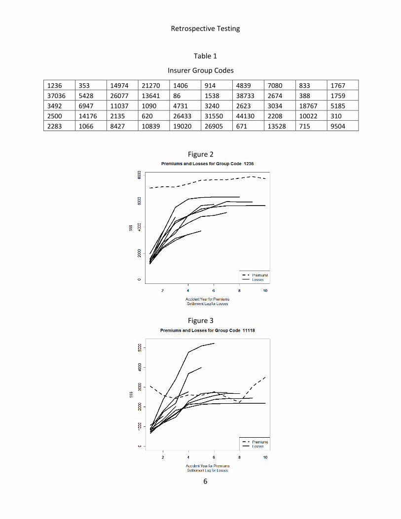
insurers that we deemed unprofitable. In the end we selected 50 insurers for this analysis.

Figure 2 shows the earned premiums and cumulative paid losses by accident year for the

first insurer we accepted, and Figure 3 shows the earned premium and losses by accident year

for the first insurer we rejected. Table 1 gives the Group Codes for all insurers included in this

analysis.


6

Table 1

Insurer Group Codes

1236 353 14974 21270 1406 914 4839 7080 833 1767

37036 5428 26077 13641 86 1538 38733 2674 388 1759

3492 6947 11037 1090 4731 3240 2623 3034 18767 5185

2500 14176 2135 620 26433 31550 44130 2208 10022 310

2283 1066 8427 10839 19020 26905 671 13528 715 9504

Figure 2

Figure 3


7

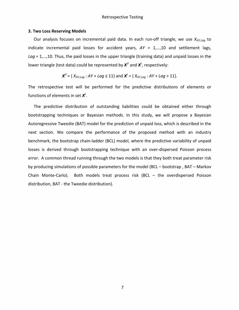
3. Two Loss Reserving Models

Our analysis focuses on incremental paid data. In each run-off triangle, we use XAY,Lag to

indicate incremental paid losses for accident years, AY = 1,…,10 and settlement lags,

Lag = 1,…,10. Thus, the paid losses in the upper triangle (training data) and unpaid losses in the

lower triangle (test data) could be represented by XU and X

L, respectively:

XU

= { XAY,Lag : AY + Lag ≤ 11} and XL = { XAY,Lag : AY + Lag > 11}.

The retrospective test will be performed for the predictive distributions of elements or

functions of elements in set XL.

The predictive distribution of outstanding liabilities could be obtained either through

bootstrapping techniques or Bayesian methods. In this study, we will propose a Bayesian

Autoregressive Tweedie (BAT) model for the prediction of unpaid loss, which is described in the

next section. We compare the performance of the proposed method with an industry

benchmark, the bootstrap chain-ladder (BCL) model, where the predictive variability of unpaid

losses is derived through bootstrapping technique with an over-dispersed Poisson process

error. A common thread running through the two models is that they both treat parameter risk

by producing simulations of possible parameters for the model (BCL – bootstrap , BAT – Markov

Chain Monte-Carlo). Both models treat process risk (BCL – the overdispersed Poisson

distribution, BAT - the Tweedie distribution).


8

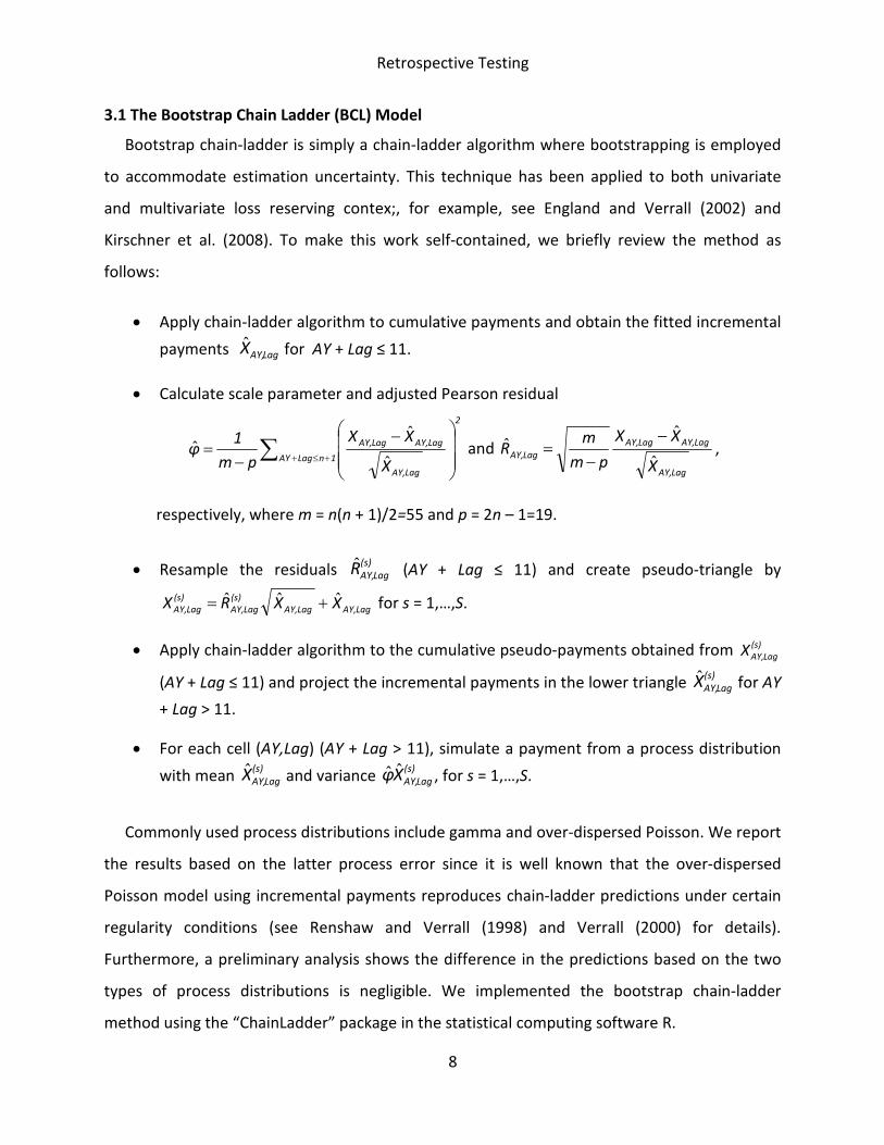
3.1 The Bootstrap Chain Ladder (BCL) Model

Bootstrap chain-ladder is simply a chain-ladder algorithm where bootstrapping is employed

to accommodate estimation uncertainty. This technique has been applied to both univariate

and multivariate loss reserving contex;, for example, see England and Verrall (2002) and

Kirschner et al. (2008). To make this work self-contained, we briefly review the method as

follows:

• Apply chain-ladder algorithm to cumulative payments and obtain the fitted incremental

payments LagAY,X̂ for AY + Lag ≤ 11.

• Calculate scale parameter and adjusted Pearson residual

2

1nLagAY

LagAY,

LagAY,LagAY,

X

XX

pm

1φ ∑ +≤+

−

−=

ˆ

ˆ

ˆ and

LagAY,

LagAY,LagAY,

LagAY,

X

XX

pm

mR

ˆ

ˆˆ

−

−= ,

respectively, where m = n(n + 1)/2=55 and p = 2n – 1=19.

• Resample the residuals (s)

LagAY,R̂ (AY + Lag ≤ 11) and create pseudo-triangle by

LagAY,LagAY,

(s)

LagAY,

(s)

LagAY, XXRX ˆˆˆ += for s = 1,…,S.

• Apply chain-ladder algorithm to the cumulative pseudo-payments obtained from (s)

LagAY,X

(AY + Lag ≤ 11) and project the incremental payments in the lower triangle (s)

LagAY,X̂ for AY

+ Lag > 11.

• For each cell (AY,Lag) (AY + Lag > 11), simulate a payment from a process distribution

with mean (s)

LagAY,X̂ and variance (s)

LagAY,Xφ ˆˆ , for s = 1,…,S.

Commonly used process distributions include gamma and over-dispersed Poisson. We report

the results based on the latter process error since it is well known that the over-dispersed

Poisson model using incremental payments reproduces chain-ladder predictions under certain

regularity conditions (see Renshaw and Verrall (1998) and Verrall (2000) for details).

Furthermore, a preliminary analysis shows the difference in the predictions based on the two

types of process distributions is negligible. We implemented the bootstrap chain-ladder

method using the “ChainLadder” package in the statistical computing software R.


9

3.2 The Bayesian Autoregressive Tweedie (BAT) Model

The objective of this model is given the observed data XU, predict the distribution of the sum of

all amounts in XL.

The high-level considerations made in formulating this model include:

1. The model should use the reported premiums as a measure of exposure. This

consideration has precedent with the Bornhuetter-Ferguson method, but it differs from

other popular models such as the chain-ladder. Given that the model uses premiums, it

should recognize that competitive conditions in the American insurance industry lead to

slowly changing loss ratios over time.

2. As the settlement lag increases, the payments follow no discernable natural pattern

other than ultimately, they approach zero.

3. The model should reflect inflationary changes in loss levels by calendar year. This

consideration has precedent with other models such as the one proposed by Barnett

and Zehnwirth (2000). The model should recognize that inflation can change slowly

over time.

4. Process risk is present and important for (AY,Lag) cells with low expected losses. In

general, the coefficient of variation of the process risk should decrease as the expected

loss increases, but it should never approach zero. Also, the process risk in the later

settlement lags should reflect the larger claims that take longer to settle.

5. The model is Bayesian. Loss reserve models tend to have many parameters. As

demonstrated by Meyers (2007a), loss reserve models fit by maximum likelihood with a

large number of parameters tend to understate the variance of the outcomes. Bayesian

approaches will correct for this by incorporating parameter risk into calculating the

variance of the outcomes. Other approaches, such as bootstrapping, also incorporate

parameter risk.


10

The unknown parameters for this model are as follows.

• ELRAY, for AY = 1,…,10. These parameters represent the expected loss ratio for

accident year AY.

• DevLag, for Lag = 1,…,10. These parameters represent the paid incremental loss

development factors for settlement lag Lag. To prevent overdeterming the model

we imposed the constraint that 10

1

1Lag

Lag

Dev=

=∑ .

• CYTi, for i = 1,…,19. These parameters represent the calendar year trend factor.

For a given (AY,Lag) cell, we have i = AY + Lag – 1. To prevent overdetermining the

model we set CYT1 = 1.

• Sev represents the claim severity for claims that settle in the 10th

settlement lag.

For Lag < 10, the claim severity is given by ( )31 (1 /10)Sev Lag⋅ − − . This expression

for the claim severity guarantees that the claim severity increases as the

settlement lag increases.

• c represents the contagion parameter as described in Meyers(2007b). Its role is to

keep the coefficient of variation of the process risk from decreasing to zero as the

expected loss increases. Its precise role will be specified in the likelihood function

below.

To allow the {ELRAY} parameters to change slowly over time, we impose the following AR(1)

structure on the parameters.

ELRAY = µA· (1 - ρA) + ρA·ELRAY-1 + εA.

From the standard properties of the AR(1) model we have that:

• The long-term average of the ELRAY parameters = µA.

• Corr(ELRAY, ELRAY-k) = ρAk.

• εA ~ N(0,σA).


11

The prior distribution of {{ELRAY},µA,ρA,σA} takes the form:

where:

• Φ is the standard normal distribution.

• f is a gamma distribution with mean 0.7 and coefficient of variation 0.18.

• g is a uniform (0,1) distribution.

• h is a gamma distribution with mean 0.025 and coefficient of variation 0.5.

We impose a similar structure on {CTYi} with the prior distribution taking the form:

where:

• Φ is the standard normal distribution.

• f is a gamma distribution with mean 1 and coefficient of variation 0.18.

• g is a uniform (0,1) distribution.

• h is a gamma distribution with mean 0.025 and coefficient of variation 0.5.

{ }( ) ( )( )10

1

2

, , , ( ) ( ) ( ) 1 |0,AY A A A A A A AY A A A AY A

AY

p ELR f g h ELR ELRµ ρ σ µ ρ σ µ ρ ρ σ−=

= ⋅ ⋅ ⋅ Φ − ⋅ − − ⋅∏

{ }( ) ( )( )10

1

2

, , , ( ) ( ) ( ) 1 |0,i C C C C C C i C C C i C

i

p CYT f g h CYT CYTµ ρ σ µ ρ σ µ ρ ρ σ−=

= ⋅ ⋅ ⋅ Φ − ⋅ − − ⋅∏


12

The prior distributions for the remaining parameters were gamma distributions with the

parameters given in Table 2. These were derived by fitting a similar model by maximum

likelihood to a large number of insurers.

Table 2

Implied

Parameter α θ Mean Std. Dev.

Sev 1.3676 136.248 186.3386 159.3400

c 0.074 0.1391 0.0103 0.0379

Dev1 15.81 0.0135 0.2137 0.0537

Dev2 42.8538 0.0059 0.2517 0.0385

Dev3 56.4944 0.0036 0.2028 0.0270

Dev4 30.4528 0.0046 0.1403 0.0254

Dev5 10.2309 0.0085 0.0870 0.0272

Dev6 5.8094 0.0083 0.0480 0.0199

Dev7 3.6954 0.0068 0.0250 0.0130

Dev8 2.3934 0.0057 0.0135 0.0087

Dev9 1.3559 0.0066 0.0090 0.0077

Dev10 0.4552 0.0200 0.0091 0.0135

The joint prior distribution for all the parameters is the product of all the individual prior

distributions given above.

We used the Tweedie distribution with index p = 1.67 to describe the process risk. For a

given (AY,Lag) cell, the expected loss is given by:

.

The scale parameter for the Tweedie distribution for each (AY,Lag) cell is given by:

.

1

,

1

AY Lag

AY Lag AY AY Lag i

i

E X Premium ELR Dev CYT+ −

=

= ⋅ ⋅ ⋅ ∏

31

,2

,

110

2

p

AY Lagp

AY Lag

LagE X Sev

c E Xp

φ

−

−

⋅ ⋅ − = + ⋅ −


13

This expression for φ can be explained by noting that the variance for the Tweedie

distribution is usually written in the form φ ·µ p. Substituting µ = E[XAY,Lag] and the value above

for φ into the expression for the Tweedie variance yields a variance of

E[XAY,Lag]/(2 - p)+c·E[XAY,Lag]2. The coefficient of variation squared is then equal to

( ),

1

2AY Lag

cE X p

+ ⋅ −

. This coefficient of variation squared decreases to c as the expected loss,

E[XAY,Lag], increases.

The likelihood function for the data2 in the upper triangle is the product of the Tweedie

density functions over all the (AY,Lag) cells in the upper triangle, XU.

With the prior distribution and the likelihood function specified above, we used the

Metropolis Hastings algorithm3 to generate a sample of size 1,000 parameter sets from the

posterior distribution.

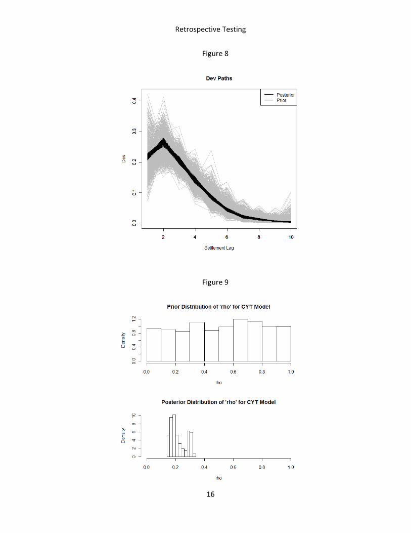
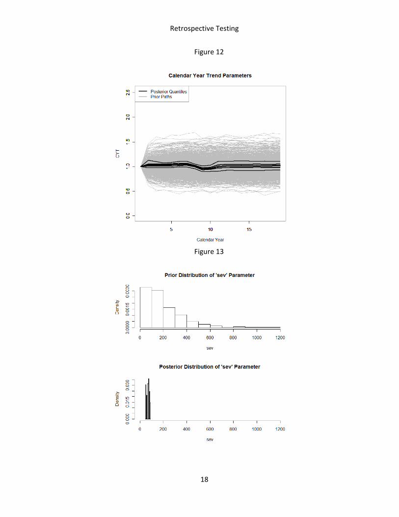
Figures 4 to 14 below graphically show how the data reduces the uncertainty in the range in

the parameters by comparing the prior and posterior distributions of the parameters. We

produced these plots using the data of the insurer with group code 914.

2 In fitting the data, we dropped all (AY,Lag) cells with negative paid incremental losses.

3 See Meyers (2009) for an explanation of the Metropolis Hastings Algorithm. For each parameter, we used a

gamma distribution with a shape parameter, α = 2,000, for the proposal density function. To obtain convergence

and guard against autocorrelation, we ran 50,000 iterations and took a sample of size 1,000 from the last 25,000

iterations.


14

Figure 4

Figure 5


15

Figure 6

Figure 7


16

Figure 8

Figure 9


17

Figure 10

Figure 11


18

Figure 12

Figure 13


19

Figure 14

For each of the 1,000 randomly selected parameter sets {{ELRAY}, {DevLag}, Sev, c}, we then

calculated the mean and variance of the Tweedie distribution of XAY,Lag for each (AY,Lag) cell in

the lower triangle and then took 10 different random simulations of . These

simulations produced 10,000 samples of this sum. Given the amount of an outstanding liability,

we calculate the cumulative probability by counting the number of simulations that are less

than or equal to it.

10 10

,

2 12

AY Lagx

AY Lag AY

X= = −∑ ∑


20

4. Retrospective Tests for Single Insurers

Loss reserve models are calibrated using the observed run-off triangle and then are used to

forecast outstanding liabilities. From the perspective of risk management, a reasonable reserve

range is of more interest to reserving actuaries and risk managers. Stochastic claims reserving

models achieve this goal by providing a best estimate as well as a variability measure of

reserves; for example, the conditional mean-squared prediction error. This paper focuses on

testing the predictive distribution of outstanding claims. We emphasize that a fair test should

be based on a retrospective evaluation using the realized claims of predictive interests. In this

study, the retrospective test will be performed at two levels: individual firm and portfolio of

insurers. This section focuses on the tests for single insurers and the next section performs tests

for multiple insurers.

At firm level, the retrospective test informs actuaries on the predictive performance of a

stochastic claims reserving method for each individual firm. For a specific insurer, we calculate

the percentile of realized unpaid losses xAY,Lag for each cell (AY,Lag) in the unobserved triangle,

by pAY,Lag = F (xAY,Lag), where F (·) denotes the predictive distribution of XAY,Lag derived from a

certain stochastic reserving method. All these pAY,Lag (AY + Lag > 11) are expected to be a

random sample of a uniformly distributed variable on [0, 1], if the model assumptions of the

stochastic reserving method are appropriate for the insurer. The uniformity of percentiles could

be visualized through graphical tools such as Probability-Probability (PP) plot, or could be easily

tested using formal statistics such as a Kolmogorov-Smirnov (KS) test.

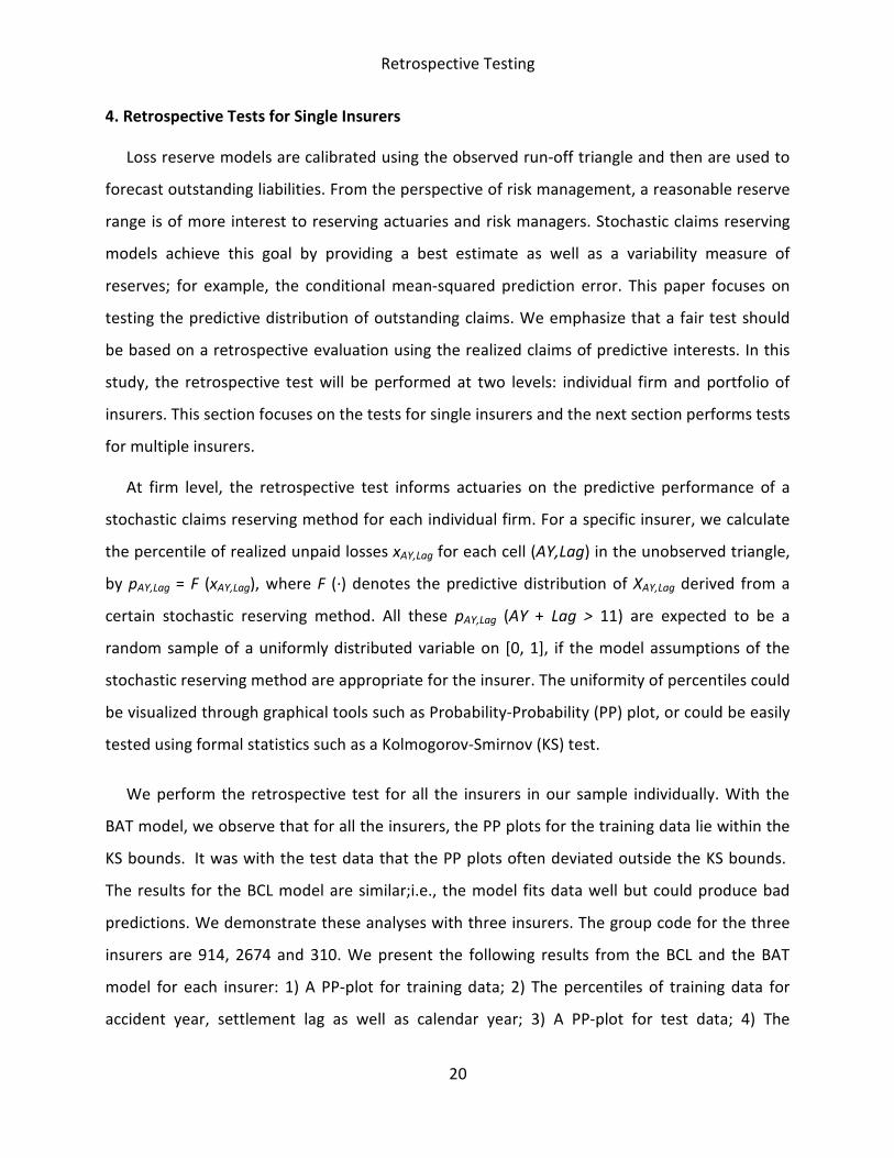
We perform the retrospective test for all the insurers in our sample individually. With the

BAT model, we observe that for all the insurers, the PP plots for the training data lie within the

KS bounds. It was with the test data that the PP plots often deviated outside the KS bounds.

The results for the BCL model are similar;i.e., the model fits data well but could produce bad

predictions. We demonstrate these analyses with three insurers. The group code for the three

insurers are 914, 2674 and 310. We present the following results from the BCL and the BAT

model for each insurer: 1) A PP-plot for training data; 2) The percentiles of training data for

accident year, settlement lag as well as calendar year; 3) A PP-plot for test data; 4) The


21

percentiles of test data for accident year, settlement lag, as well as calendar year. If the model

fits well, we should expect the PP-plot to lie along the 45o line, and to see no pattern in the

remaining plots by accident year, settlement lag or calendar year. The results are summarized

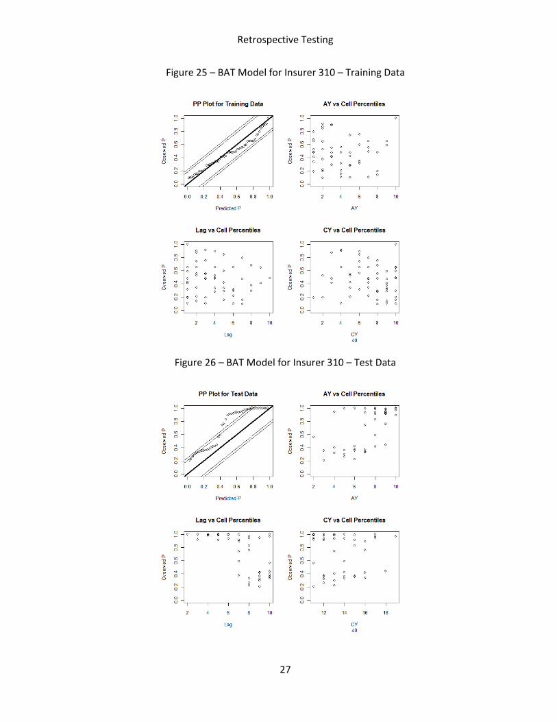
in Figures 15 – 26.

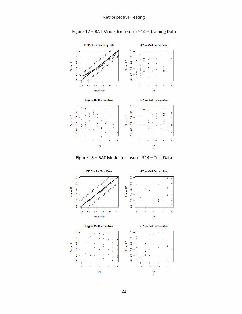
In terms of goodness-of-fit, the PP-plots of training data suggest that both BCL and BAT

models fit training data well for all insurers. When examining the test data, the retrospective

test shows that the PP plots of both models are within the KS bounds for insurer 914, but

outside the KS bounds for insurer 310. For insurer 2764, the BCL model provides better

predictive distribution than the BAT model. We attribute such observations to the potential

overfitting of the two loss reserving models. Though not reported here, our analysis showed

that the loss development of insurer 914 is rather stable over time, while the payments for

insurer 2764 and 310 are more volatile from year to year, especially for insurer 310. The higher

variability explains the poor predictive performance of both models on insurer 310. Another

factor affecting the predictive performance of loss reserving models appears to be an

environmental change in the projecting period. Our analysis in the next section shows that the

BCL model somehow did a better job in the perceived changing environment.


22

Figure 15 – BCL Model for Insurer 914 – Training Data

Figure 16 – BCL Model for Insurer 914 – Test Data


23

Figure 17 – BAT Model for Insurer 914 – Training Data

Figure 18 – BAT Model for Insurer 914 – Test Data


24




25




26




27




28

5. Retrospective Tests for Multiple Insurers

The retrospective test could be performed for a portfolio of insurers as well. At portfolio

level, the retrospective test helps detect the potential under or over reserving issue if one

single stochastic method is applied to all insurers in the portfolio. The same idea could be

generalized to the industry level. Considering a portfolio of N property-casualty insurers, we

implement the test using total reserves. Specifically, for the kth (k = 1,…,N) insurer in the

portfolio, we calculate the percentiles of realized total unpaid losses in the lower triangle

)F(rpTot

k

Tot

k = . Here F(·) and rk indicate the corresponding predictive distribution and realized

unpaid losses, respectively. Whether the stochastic reserving method is suitable for the insurer

portfolio could be answered by examining the uniformity of Tot

kp .

This section compares the predictions of the Bayesian Autoregressive Tweedie (BAT) model

and the Bootstrap Chain Ladder (BCL) model. Our data also includes the reserve that each

insurer posted in the 1997 Annual Statement. The reserves posted by the insurer differ from

the models in that they are not tied to any particular method or model and can reflect insurer

judgment. Also, it is not difficult to imagine the various incentives that can influence the

judgments in either direction.

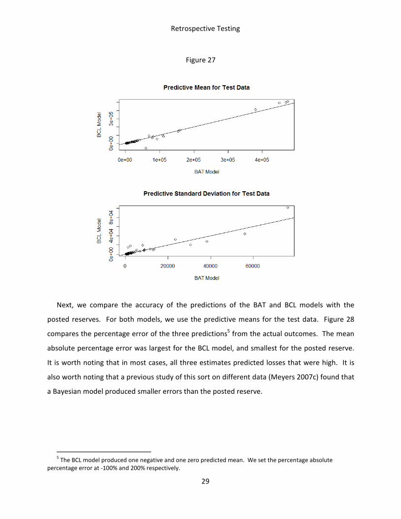
Figure 27 compares the predictive means and standard deviations of the total outstanding

losses using the BAT and BCL methods. This figure indicates that for the most part, the

predictive means are fairly close4. There are a noticeable number of instances where the

predictive standard deviation is smaller for the BAT model.

4 In one case the mechanical application of the BCL model produced a negative mean because of a negative

incremental paid loss. Any actuary would reject this result, in practice. The BAT model dropped any cell that

contained a negative incremental paid loss.


29

Figure 27

Next, we compare the accuracy of the predictions of the BAT and BCL models with the

posted reserves. For both models, we use the predictive means for the test data. Figure 28

compares the percentage error of the three predictions5 from the actual outcomes. The mean

absolute percentage error was largest for the BCL model, and smallest for the posted reserve.

It is worth noting that in most cases, all three estimates predicted losses that were high. It is

also worth noting that a previous study of this sort on different data (Meyers 2007c) found that

a Bayesian model produced smaller errors than the posted reserve.

5 The BCL model produced one negative and one zero predicted mean. We set the percentage absolute

percentage error at -100% and 200% respectively.


30

Figure 28

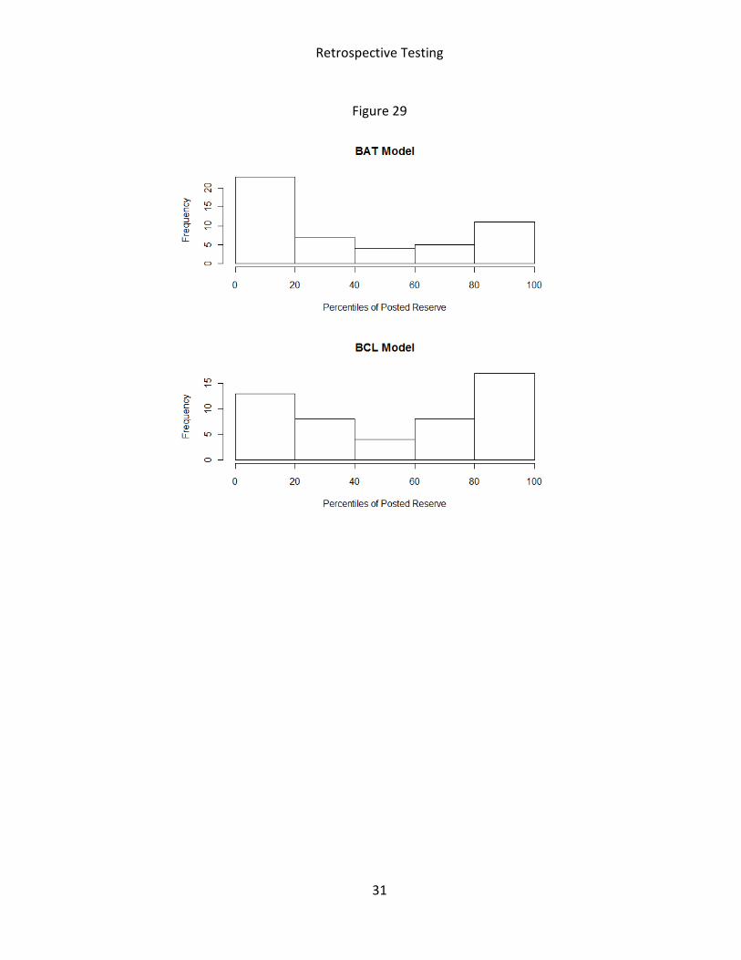
When a stochastic loss reserve analysis is performed, a question commonly asked by

actuaries is “What percentile should one post a reserve.” While we do not intend to answer

that question, we can use the BAT and the BCL models to estimate the percentiles of the actual

posted reserve. Figure 29 provides the results. It appears that many insurers post conservative

estimates, while many others (correctly as it turns out) posted lower than expected reserves.


31

Figure 29


32

If a loss reserve model is appropriate for all insurers, the predicted percentiles of the data

should be uniformly distributed. Figure 30 provides histograms for both models with the

training data and Figure 31 provides histograms for both models on the test data. All four

histograms indicate non-uniformity of the predicted percentiles. It should come as no surprise

that the percentiles tend to be around the middle ranges on the training. Because of the high

parameter to data point ratio, we attribute this to overfitting. We interpret the results for the

test data as an indication that either: (1) something changed in the environment that resulted

in lower claim settlements; or (2) no single model should be expected to apply for all insurers.

It appears that, for whatever reason, the BCL did a better job of picking up that environmental

change.

Figure 30


33

Figure 31

6. Concluding Remarks

The primary purpose of this paper was to introduce a new database that can be used to test

predictive distributions from different stochastic loss reserve models. We emphasized the

retrospective tests based on realized payments in the projecting periods. We then performed

some tests on an established model, bootstrap chain ladder (BCL) model, and a proposed new

model, Bayesian Autoregressive Tweedie (BAT) model. At this point in time, we are not ready

to declare a winner. These models, and perhaps other models, should be tested on other lines

of insurance. And the database is there that will permit further testing.

This particular study suggests that there might be environmental changes that no single

model can identify. If this continues to hold, the actuarial profession cannot rely solely on

stochastic loss reserve models to manage its reserve risk. We need to develop other risk

management strategies that do deal with unforeseen environmental changes.


34

References:

England, P. and R. Verrall (2002). Stochastic claims reserving in general insurance. British

Actuarial Journal 8 (3), 443-518.

Kirschner, G., C. Kerley, and B. Isaacs (2008). Two approaches to calculating correlated

reserve indications across multiple lines of business. Variance 2 (1), 15-38.

Meyers, Glenn G. (2007a). Thinking Outside the Triangle. ASTIN Colloquium 2007.

http://www.actuaries.org/ASTIN/Colloquia/Orlando/Papers/Meyers.pdf

Meyers, Glenn G. (2007b). The Common Shock Model for Correlated Insurance

Losses, Variance 1:1, pp. 40-52.

Meyers, Glenn G. (2007c). Estimating Predictive Distributions for Loss Reserve

Models, Variance 1:2, pp. 248-272.

Meyers, Glenn G. (2009). Bayesian Analysis with the Metropolis Hastings Algorithm, The

Actuarial Review, November 2009.

http://www.casact.org/newsletter/index.cfm?fa=viewart&id=5866

Renshaw, A. and R. Verrall (1998). A stochastic model underlying the chain-ladder technique.

British Actuarial Journal 4 (4), 903-923.

Shi, P., S. Basu, and G. G. Meyers (2011). A Bayesian Log-normal Model for Multivariate Loss

Reserving. Submitted for Publication.

Taylor, G. (2000). Loss Reserving: An Actuarial Perspective. Kluwer Academic Publishers.

Verrall, R. (2000). An investigation into stochastic claims reserving models and the chain-

ladder technique. Insurance: Mathematics and Economics 26 (1), 91-99.

Wüthrich, M. and M. Merz (2008). Stochastic Claims Reserving Methods in Insurance. John

Wiley & Sons.


35

Appendix

This appendix describes the data set of loss triangles that we prepared for claims reserving

studies. The data cover major personal and commercial lines of business from U.S. property

casualty insurers. We extract the claims data from Schedule P – Analysis of Losses and Loss

Expenses in the National Association of Insurance Commissioners (NAIC) database.

A.1 Schedule P

NAIC Schedule P contains information on claims for major personal and commercial lines for

all property-casualty insurers that write business in US. Some parts have sections that separate

occurrence from claims made coverages. We focus on the following six lines: (1) private

passenger auto liability/medical; (2) commercial auto/truck liability/medical; (3) worker’s

compensation; (4) medical malpractice – claims made; (5) other liability – occurrence; (6)

product liability – occurrence.

For each of the above six lines, the variables to be included in the dataset are pulled from

three different parts in Schedule P, including:

Part 1 - Earned premium and some summary loss data

Part 2 - Incurred net loss triangles

Part 3 - Paid net loss triangles

Part 4 - Bulk and IBNR Reserves

A.2 Data Preparation

The triangles consist of losses net of reinsurance, and quite often insurer groups have

mutual reinsurance arrangements between the companies within the group. Consequently, we

focus on records for single entities in the data preparation, be they insurer groups or true single

insurers. The process of data preparation takes three steps:

Step I: Pull triangle data from Schedule P of year 1997. Each triangle includes claims of 10

accident years (1988-1997) and 10 development lags. This data was the training data used for

model development.


36

Step II: Square the triangles from Schedule P of year 1997 with outcomes from Schedule P of

subsequent years. Specifically, the data for accident year 1989 was pulled from Schedule P of

year 1998, the data for accident year 1990 was pulled from Schedule P of year 1999, ……, the

data for accident year 1997 was pulled from Schedule P of year 2006. The data in the lower

triangles could be used for model validation purposes.

Step III: We performed a preliminary analysis to ensure the quality of the dataset. An insurer

is retained in the final dataset if all following criteria are satisfied: (1) the insurer is available in

both Schedule P of year 1997 and subsequent years; (2) the observations (10 accident years

and 10 development lags) are complete for the insurer; (3) the claims from Schedule P of year

1997 match those from subsequent years.


37

A.3 Final Dataset

As a final product, we provide a dataset that contains run-off triangles of six lines of business

for all U.S. property casualty insurers. The triangle data correspond to claims of accident year

1988 – 1997 with 10 years development lag. Both upper and lower triangles are included so

that one could use the data to develop a model and then test its performance retrospectively. A

list of variables in the data is as follows:

Table A.1. Description of Variables

Variable Description

GRCODE NAIC company code (including insurer groups and single insurers)

GRNAME NAIC company name (including insurer groups and single insurers)

AccidentYear Accident year (calendar year)

DevelopmentYear Development year (calendar year)

DevelopmentLag Development year - Incurral year + 1

IncurLoss_ Incurred losses and allocated expenses reported at year end

CumPaidLoss_ Cumulative and paid losses and allocated expenses at year end

EarnedPremD_ Premiums earned at incurral year - direct and assumed

EarnedPremC_ Premiums earned at incurral year - ceded

EarnedPremN_ Premiums earned at incurral year - net

Single 1 indicates a single entity, 0 indicates a group insurer

"_" Refers to lines of business

B Private passenger auto liability/medical

C commercial auto/truck liability/medical

D Workers' compensation

F2 Medical malpractice - Claims made

H1 Other liability - Occurrence

R1 Products liability - Occurrence

the retrospective testing of stochastic loss reserve models

Documents