Working Paper Series

The Rise and Fall of Income Inequality in

Mexico, 1989–2010

Raymundo Campos

Gerardo Esquivel

Nora Lustig

ECINEQ WP 2012 – 267

ECINEQ 2012 – 267

September 2012

www.ecineq.org

The Rise and Fall of Income Inequality in

Mexico, 1989–2010*

Raymundo Campos,

Gerardo Esquivel

Nora Lustig*

Abstract

Inequality in Mexico rose between 1989 and 1994 and declined between 1994 and 2010. We examine the role of market forces (demand and supply of labour by skill), institutional factors (minimum wages and unionization rate), and public policy (cash transfers) in explaining changes in inequality. We apply the ‘re-centered influence function’ method to decompose changes in hourly wages into characteristics and returns. The main driver is changes in returns. Returns rose (1989-1994) due to institutional factors and labour demand. Returns declined (1994-2006) due to changes in supply and --to a lesser extent--in demand; institutional factors were not relevant. Government transfers contributed to the decline in inequality, especially after 2000.

Keywords: inequality; wages; disposable income; labour markets; Mexico.

JEL Classification: D31, J20, J31, O54.

*This study is reproduced here by permission of UNU-WIDER; the latter commissioned the original research and holds copyright thereon. Paper prepared for UNU-WIDER’s project ‘The New Policy Model, Inequality and Poverty in Latin America: Evidence from the Last Decade and Prospects for the Future, coordinated by Giovanni Andrea Cornia. An earlier version of this paper was presented at the project’s conference in Buenos Aires, Argentina, 1-3 September 2011. The authors are grateful to Giovanni Andrea Cornia, Richard Freeman and Stefan Klasen as well as the rest of the conference participants for their very useful comments. The authors also wish to thank Alma S. Santillan as well as Mayra Paulina Salazar and Emily Travis for their excellent research assistantship. All errors and omissions remain the authors’ sole responsibility.

*Contact details: Raymundo Campos and Gerardo Esquivel are professors at the Center for Economic Studies, El Colegio de Mexico; and, Nora Lustig is Samuel Z. Stone Professor of Latin American Economics, Tulane University and nonresident senior fellow at the Center for Global Development and Inter-American Dialogue. Emails: rmcampos@colmex.mx; gesquive @colmex.mx; nlustig@tulane.edu.

1 Introduction

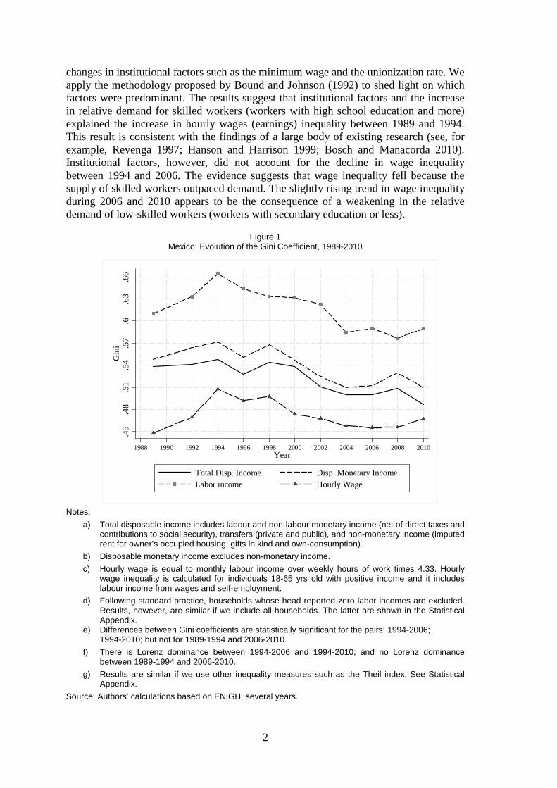
During the last twenty years, the evolution of inequality in Mexico followed two distinct patterns (Figure 1): it rose between 1989 and the mid-1990s and declined between the mid-1990s and 2010. All in all, the Gini coefficient for per capita (disposable monetary) income rose from 0.548 to 0.571 between 1989 and 1994, and declined to 0.510 in 2010.1 The period of declining inequality can also be divided in two: 1994-2006, when inequality decidedly fell (Gini fell from 0.571 to 0.512); and, 2006-10, when the decline in inequality loses its steam.2

Esquivel, Lustig and Scott (2010) show that changes in labour income and non-labour income inequality were equalizing for the period 1996-2006 and that the decline in labour income inequality was by far the most important proximate determinant of the observed decline in overall inequality.3 Given the importance of labour market inequality dynamics in explaining the trend in overall inequality, this paper concentrates on analysing the more ‘fundamental’ determinants of labour income inequality. In particular, it examines the role of market forces (relative demand and supply of labour by skill) and institutional factors (minimum wages and unionization rate) in explaining changes in the distribution of hourly wages. It also extends the analysis to 2010. By doing so, it examines the factors that may account for the pause (reversal?) in the decline in inequality momentum between 2006 and 2010.

More specifically, this paper applies the (‘re-centred influence function’ or RIF) method proposed by Firpo, Fortin and Lemieux (2009) to decompose changes in hourly wages into characteristics and returns effects.4 Results reveal that the main driver behind the rise and decline in earnings inequality are changes in returns.5 Given the prominence of the returns effect, the paper proceeds to analyse the determinants of the evolution of relative returns in turn.

Changes in returns can be due to changes in the relative demand and supply of workers of different characteristics (in particular, education used as a proxy for skill) and/or

1 As is the case with practically all inequality estimates based on household surveys, the Gini coefficients presented here are probably an underestimation of ‘true’ levels of inequality because of the significant under-reporting of incomes and consumption at the top of the distribution.

2 The years 1996 and 2008 are atypical because the country was experiencing a crisis. In this paper we do not attempt to explain which factors determine inequality dynamics when there was a crisis.

3 The reduction in labour income inequality (leaving out the interaction terms) accounted for 87.1 percent of the decline in inequality in 1996-2000 and for 65.5 percent of the decline in 2000-06.

4 Although the RIF procedure was published in 2009, there have been several papers employing it. See Chi, Li and Yu (2011) for an application of wage inequality in China; Thu Le and Booth (2010) for a decomposition in Vietnam; and Holmes and Mayhew (2010) for a labour market analysis in the UK.

5 In fact, changes in characteristics were unequalizing during the period of declining inequality (1994-2006) in spite of the reduction in the Gini coefficient for education. This suggests a persistence of what Bourguignon, Ferreira and Lustig (2005) called the ‘paradox of progress’ which Legovini, Bouillon and Lustig (2005) found in Mexico for the period 1984-94.

2

changes in institutional factors such as the minimum wage and the unionization rate. We apply the methodology proposed by Bound and Johnson (1992) to shed light on which factors were predominant. The results suggest that institutional factors and the increase in relative demand for skilled workers (workers with high school education and more) explained the increase in hourly wages (earnings) inequality between 1989 and 1994. This result is consistent with the findings of a large body of existing research (see, for example, Revenga 1997; Hanson and Harrison 1999; Bosch and Manacorda 2010). Institutional factors, however, did not account for the decline in wage inequality between 1994 and 2006. The evidence suggests that wage inequality fell because the supply of skilled workers outpaced demand. The slightly rising trend in wage inequality during 2006 and 2010 appears to be the consequence of a weakening in the relative demand of low-skilled workers (workers with secondary education or less).

Figure 1 Mexico: Evolution of the Gini Coefficient, 1989-2010

Notes:

a) Total disposable income includes labour and non-labour monetary income (net of direct taxes and contributions to social security), transfers (private and public), and non-monetary income (imputed rent for owner’s occupied housing, gifts in kind and own-consumption).

b) Disposable monetary income excludes non-monetary income.

c) Hourly wage is equal to monthly labour income over weekly hours of work times 4.33. Hourly wage inequality is calculated for individuals 18-65 yrs old with positive income and it includes labour income from wages and self-employment.

d) Following standard practice, households whose head reported zero labor incomes are excluded. Results, however, are similar if we include all households. The latter are shown in the Statistical Appendix.

e) Differences between Gini coefficients are statistically significant for the pairs: 1994-2006; 1994-2010; but not for 1989-1994 and 2006-2010.

f) There is Lorenz dominance between 1994-2006 and 1994-2010; and no Lorenz dominance between 1989-1994 and 2006-2010.

g) Results are similar if we use other inequality measures such as the Theil index. See Statistical Appendix.

Source: Authors’ calculations based on ENIGH, several years.

.45

.48

.51

.54

.57

.6.6

3.6

6G

ini

1988 1990 1992 1994 1996 1998 2000 2002 2004 2006 2008 2010Year

Total Disp. Income Disp. Monetary IncomeLabor income Hourly Wage

3

As mentioned above, another factor behind the decline in overall inequality was the decline in non-labour income inequality (Esquivel, Lustig and Scott). Non-labour income is a very heterogeneous category. It includes all forms of income from capital (although grossly under-reported in household surveys), pensions from contributory systems, private transfers (remittances, in particular) and government transfers. An application of the Lerman and Yitzhaki (1985) decomposition to the Mexican data showed that income from capital is always unequalizing while incomes from remittances and government transfers are always equalizing. The importance of government transfers as an equalizing factor has risen considerable over time. The fiscal incidence analysis by López-Calva, Lustig and Scott (2012) also underscores the growing importance of government transfers to reduce inequality and poverty.

In this paper we use the Gini coefficient as our preferred measure of inequality.6 This measure satisfies all the desirable properties of an inequality indicator,7 and is decomposable by proximate determinants as well as income sources.8 We use disposable monetary income per capita unless specified otherwise.9 All of our estimates use information from the National Survey of Household Incomes and Expenditures (ENIGH, for its acronym in Spanish) for 1989, 1992, 1994, 1996, 2000, 2006, 2008 and 2010.10 The surveys capture income net of taxes and contributions to social security and include government and private transfers (remittances).

2 Proximate determinants of overall inequality

Figure 1 shows the evolution of income inequality for several income measures. Measures of inequality at the household level include total disposable income (labour and non-labour income, transfers both public and private, and non-monetary income like imputed rent and autoconsumption), monetary disposable income (total income minus non-monetary income), and labour income. The graph also includes hourly wage inequality at the individual level.11 All measures show the same pattern: a rise in income

6 Other measures of inequality such as the Theil index show similar trends as those described in the text. See the Statistical Appendix.

7 These principles are: (i) adherence to the Pigou-Dalton transfer principle, (ii) symmetry, (iii) independence of scale, (iv) homogeneity, and (v) decomposability.

8 Although it is not additively decomposable as the Theil index.

9 Income includes labour income and non-labour income. The former includes all the income that is reported as labour income in ENIGH, including labour income from the self-employed. Non-labour income includes incomes from own businesses, incomes from assets (including capital gains) pensions (public and private) and public transfers (Oportunidades and Procampo) and private transfers (e.g., remittances) as well as––when indicated––Non-monetary income (imputed rent on owner occupied housing and consumption of own production, common in poor rural areas). Official poverty measures in Mexico use net current income; that is, capital gains and gifts and in-kind transfers to other households are subtracted from current total income. Current monetary income, the concept used in the decomposition of inequality by source presented here, does not include non-monetary income and consumption of own production (common in poor rural areas) and excludes capital gains.

10 In Spanish, Encuesta Nacional de Ingresos y Gastos de los Hogares (ENIGH). Although the 1989 survey is less comparable, we present results related to the factors behind the rise in inequality between 1989-94.

11 Hourly wages include hourly earnings for salaried workers and the self-employed. All calculations use sampling weights in order to generalize the results to the full population. As commonly employed in

4

inequality between 1989 and the mid-1990s and a decline in inequality between the mid-1990s and the mid-2000s. Between the mid-2000s and 2010, however, the pattern is less clear. For instance, overall (wage) inequality rose (fell) in 2008 and declined (rose) in 2010.

A useful starting point in the analysis of the determinants of inequality is to decompose the Gini coefficient into its main components and examine their contribution. Here we disaggregate total (monetary) income into labour income, income from capital12 (profits, interests, rents, etc.), private transfers (primarily remittances) and government transfers. Using the Lerman and Yitzhaki (1985) method we can distinguish between the inequality increasing and inequality decreasing components.13 The marginal contribution to total inequality of each component k is shown to depend on its own Gini coefficient (���, the size of its share in total income (��� and the correlation between the component and total income (���. Furthermore, one can show that the per cent change in inequality resulting from a marginal percentage change in income source k is equal to:14

�����

�

������

�� ��

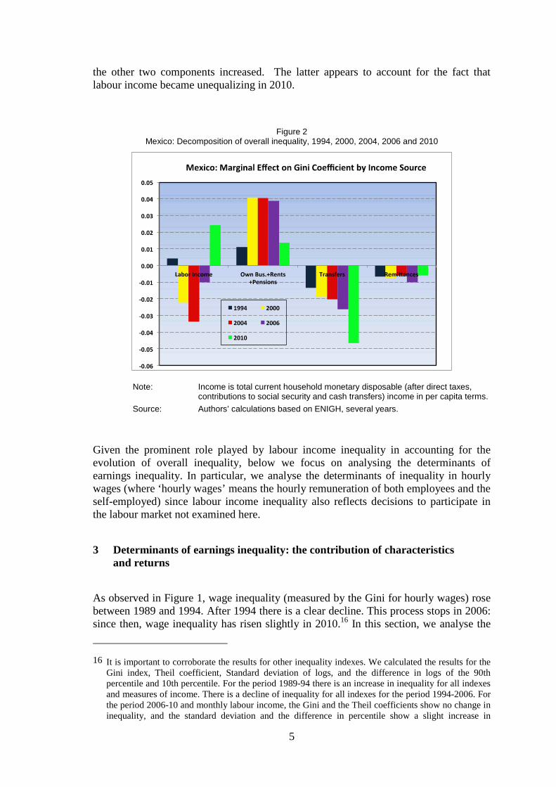
Figure 2 shows the results of applying the decomposition to 1994, 2000, 2004, 2006 and 2010. The contribution of income from ‘capital’ (own business, income from property, financial income and contributory pensions), as expected, is always inequality increasing whereas remittances and government transfers are always inequality reducing. Contribution of government transfers is higher than that of remittances and it has grown significantly over time. Income from capital represents, roughly, 20 per cent of total income; income from remittances and government transfers, the remaining 20 per cent.

Labour income, which represents more than 60 per cent of total income, does not show a definite pattern. It was inequality increasing in 1994 and very much so in 2010 but it was inequality reducing in 2000, 2006 and 2004.15 Between 1994 and 2006, the Gini coefficient of labour income fell, while the two other components (the share of labour income in total income and the correlation of labour and total income) remained basically constant. Between 2006 and 2010 there is practically no change in the Gini but

the literature of labour economics (see, for example, Autor, Katz and Kearney 2008; Card and DiNardo 2002), calculations of hourly wage inequality employ as weight the product of the sampling weight times weekly hours of work.

12 This source of income is subject to severe underreporting as incomes derived from capital at the top are not really captured in the household surveys (in Mexico and everywhere else). Here pensions from contributory systems are included under income derived from capital. Pensions are treated as income from savings, so to speak. There are a number of reasons for not including them in government transfers but this is not the place to discuss them. For more, see Lustig (2011a).

13 See also Stark, O., J. E. Taylor, and S. Yitzhaki (1986).

14 For more details see appendix.

15 These results are slightly different from those presented in Esquivel (2011) and Esquivel, Lustig and Scott (2010), due to revisions in the data and in the definitions of income.

5

the other two components increased. The latter appears to account for the fact that labour income became unequalizing in 2010.

Figure 2 Mexico: Decomposition of overall inequality, 1994, 2000, 2004, 2006 and 2010

Note: Income is total current household monetary disposable (after direct taxes, contributions to social security and cash transfers) income in per capita terms.

Source: Authors’ calculations based on ENIGH, several years.

Given the prominent role played by labour income inequality in accounting for the evolution of overall inequality, below we focus on analysing the determinants of earnings inequality. In particular, we analyse the determinants of inequality in hourly wages (where ‘hourly wages’ means the hourly remuneration of both employees and the self-employed) since labour income inequality also reflects decisions to participate in the labour market not examined here.

3 Determinants of earnings inequality: the contribution of characteristics and returns

As observed in Figure 1, wage inequality (measured by the Gini for hourly wages) rose between 1989 and 1994. After 1994 there is a clear decline. This process stops in 2006: since then, wage inequality has risen slightly in 2010.16 In this section, we analyse the

16 It is important to corroborate the results for other inequality indexes. We calculated the results for the Gini index, Theil coefficient, Standard deviation of logs, and the difference in logs of the 90th percentile and 10th percentile. For the period 1989-94 there is an increase in inequality for all indexes and measures of income. There is a decline of inequality for all indexes for the period 1994-2006. For the period 2006-10 and monthly labour income, the Gini and the Theil coefficients show no change in inequality, and the standard deviation and the difference in percentile show a slight increase in

6

main determinants of the observed trends in wage inequality. We do this by applying the decomposition methodology proposed by Firpo, Fortin and Lemieux (2009).

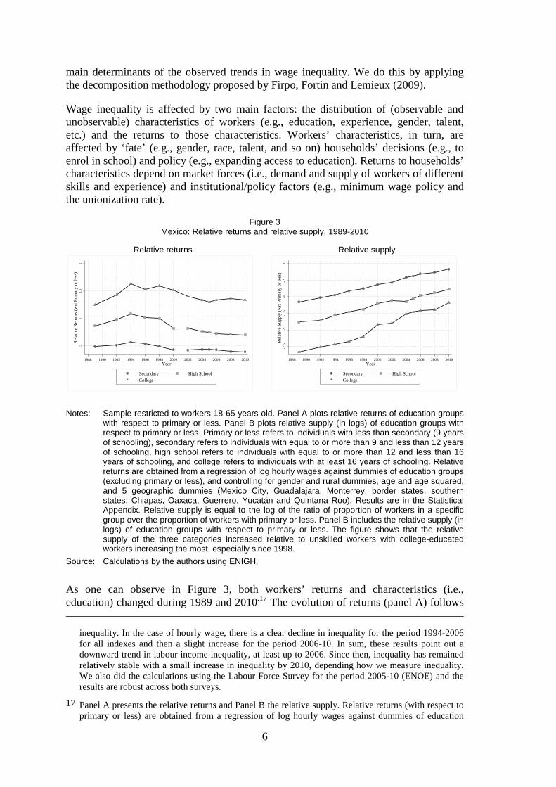
Wage inequality is affected by two main factors: the distribution of (observable and unobservable) characteristics of workers (e.g., education, experience, gender, talent, etc.) and the returns to those characteristics. Workers’ characteristics, in turn, are affected by ‘fate’ (e.g., gender, race, talent, and so on) households’ decisions (e.g., to enrol in school) and policy (e.g., expanding access to education). Returns to households’ characteristics depend on market forces (i.e., demand and supply of workers of different skills and experience) and institutional/policy factors (e.g., minimum wage policy and the unionization rate).

Figure 3 Mexico: Relative returns and relative supply, 1989-2010

Relative returns Relative supply

Notes: Sample restricted to workers 18-65 years old. Panel A plots relative returns of education groups with respect to primary or less. Panel B plots relative supply (in logs) of education groups with respect to primary or less. Primary or less refers to individuals with less than secondary (9 years of schooling), secondary refers to individuals with equal to or more than 9 and less than 12 years of schooling, high school refers to individuals with equal to or more than 12 and less than 16 years of schooling, and college refers to individuals with at least 16 years of schooling. Relative returns are obtained from a regression of log hourly wages against dummies of education groups (excluding primary or less), and controlling for gender and rural dummies, age and age squared, and 5 geographic dummies (Mexico City, Guadalajara, Monterrey, border states, southern states: Chiapas, Oaxaca, Guerrero, Yucatán and Quintana Roo). Results are in the Statistical Appendix. Relative supply is equal to the log of the ratio of proportion of workers in a specific group over the proportion of workers with primary or less. Panel B includes the relative supply (in logs) of education groups with respect to primary or less. The figure shows that the relative supply of the three categories increased relative to unskilled workers with college-educated workers increasing the most, especially since 1998.

Source: Calculations by the authors using ENIGH.

As one can observe in Figure 3, both workers’ returns and characteristics (i.e., education) changed during 1989 and 2010.17 The evolution of returns (panel A) follows

inequality. In the case of hourly wage, there is a clear decline in inequality for the period 1994-2006 for all indexes and then a slight increase for the period 2006-10. In sum, these results point out a downward trend in labour income inequality, at least up to 2006. Since then, inequality has remained relatively stable with a small increase in inequality by 2010, depending how we measure inequality. We also did the calculations using the Labour Force Survey for the period 2005-10 (ENOE) and the results are robust across both surveys.

17 Panel A presents the relative returns and Panel B the relative supply. Relative returns (with respect to primary or less) are obtained from a regression of log hourly wages against dummies of education

.51

1.5

2R

elat

ive

Re

turn

s (w

rt P

rimar

y or

less

)

1988 1990 1992 1994 1996 1998 2000 2002 2004 2006 2008 2010Year

Secondary High SchoolCollege

-2.5

-2-1

.5-1

-.5

0R

elat

ive

Sup

ply

(wrt

Prim

ary

or

less

)

1988 1990 1992 1994 1996 1998 2000 2002 2004 2006 2008 2010Year

Secondary High SchoolCollege

7

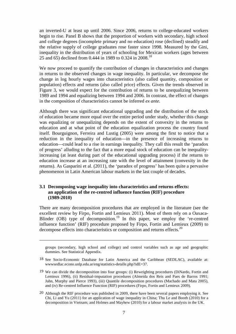
an inverted-U at least up until 2006. Since 2006, returns to college-educated workers begin to rise. Panel B shows that the proportion of workers with secondary, high school and college degrees (incomplete primary and no education) rose (declined) steadily and the relative supply of college graduates rose faster since 1998. Measured by the Gini, inequality in the distribution of years of schooling for Mexican workers (ages between 25 and 65) declined from 0.444 in 1989 to 0.324 in 2008.18

We now proceed to quantify the contribution of changes in characteristics and changes in returns to the observed changes in wage inequality. In particular, we decompose the change in log hourly wages into characteristics (also called quantity, composition or population) effects and returns (also called price) effects. Given the trends observed in Figure 3, we would expect for the contribution of returns to be unequalizing between 1989 and 1994 and equalizing between 1994 and 2006. In contrast, the effect of changes in the composition of characteristics cannot be inferred ex ante.

Although there was significant educational upgrading and the distribution of the stock of education became more equal over the entire period under study, whether this change was equalizing or unequalizing depends on the extent of convexity in the returns to education and at what point of the education equalization process the country found itself. Bourguignon, Ferreira and Lustig (2005) were among the first to notice that a reduction in the inequality of education––in the presence of increasing returns to education––could lead to a rise in earnings inequality. They call this result the ‘paradox of progress’ alluding to the fact that a more equal stock of education can be inequality-increasing (at least during part of the educational upgrading process) if the returns to education increase at an increasing rate with the level of attainment (convexity in the returns). As Gasparini et al. (2011), the ‘paradox of progress’ has been quite a pervasive phenomenon in Latin American labour markets in the last couple of decades.

3.1 Decomposing wage inequality into characteristics and returns effects: an application of the re-centred influence function (RIF) procedure (1989-2010)

There are many decomposition procedures that are employed in the literature (see the excellent review by Firpo, Fortin and Lemieux 2011). Most of them rely on a Oaxaca-Blinder (OB) type of decomposition.19 In this paper, we employ the ‘re-centred influence function’ (RIF) procedure proposed by Firpo, Fortin and Lemieux (2009) to decompose effects into characteristics or composition and returns effects.20

groups (secondary, high school and college) and control variables such as age and geographic dummies. See Statistical Appendix.

18 See Socio-Economic Database for Latin America and the Caribbean (SEDLAC), available at: wwwsedlac.econo.unlp.edu.ar/eng/statistics-detalle.php?idE=37.

19 We can divide the decomposition into four groups: (i) Reweighting procedures (DiNardo, Fortin and Lemieux 1996), (ii) Residual-imputation procedures (Almeida dos Reis and Paes de Barros 1991; Juhn, Murphy and Pierce 1993), (iii) Quantile decomposition procedures (Machado and Mata 2005), and (iv) Re-centred Influence Function (RIF) procedures (Firpo, Fortin and Lemieux 2009).

20 Although the RIF procedure was published in 2009, there have been several papers employing it. See Chi, Li and Yu (2011) for an application of wage inequality in China; Thu Le and Booth (2010) for a decomposition in Vietnam; and Holmes and Mayhew (2010) for a labour market analysis in the UK.

8

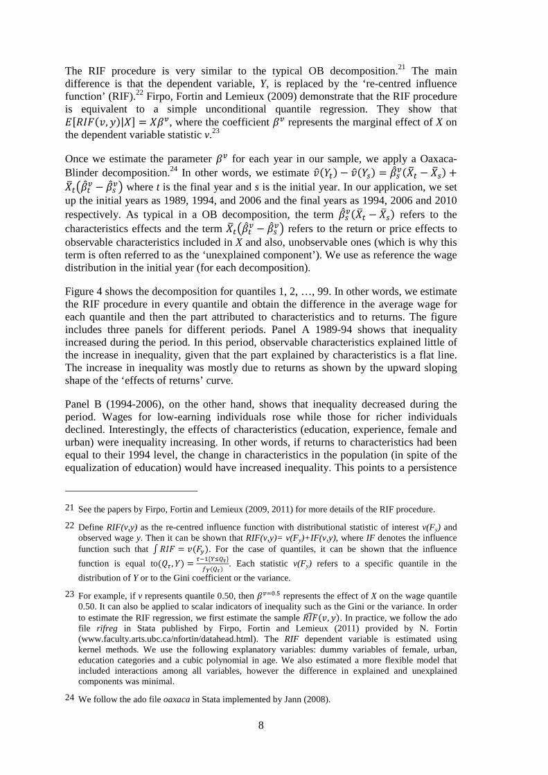
The RIF procedure is very similar to the typical OB decomposition.21 The main difference is that the dependent variable, Y, is replaced by the ‘re-centred influence function’ (RIF).22 Firpo, Fortin and Lemieux (2009) demonstrate that the RIF procedure is equivalent to a simple unconditional quantile regression. They show that � �����, ��|�� ���, where the coefficient �� represents the marginal effect of X on the dependent variable statistic v.23

Once we estimate the parameter �� for each year in our sample, we apply a Oaxaca-Blinder decomposition.24 In other words, we estimate ������ � ������ ���

����� � ���� ��������

� � ���� where t is the final year and s is the initial year. In our application, we set

up the initial years as 1989, 1994, and 2006 and the final years as 1994, 2006 and 2010 respectively. As typical in a OB decomposition, the term ���

����� � ���� refers to the characteristics effects and the term �������

� � ���� refers to the return or price effects to

observable characteristics included in X and also, unobservable ones (which is why this term is often referred to as the ‘unexplained component’). We use as reference the wage distribution in the initial year (for each decomposition).

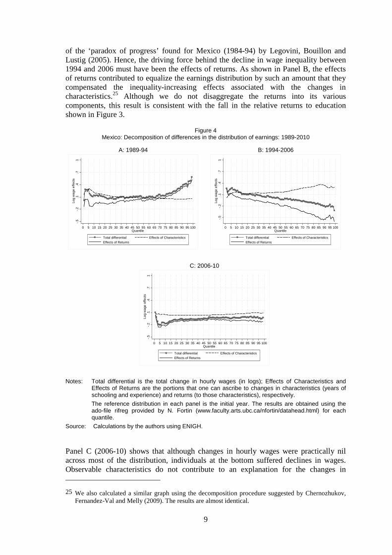
Figure 4 shows the decomposition for quantiles 1, 2, …, 99. In other words, we estimate the RIF procedure in every quantile and obtain the difference in the average wage for each quantile and then the part attributed to characteristics and to returns. The figure includes three panels for different periods. Panel A 1989-94 shows that inequality increased during the period. In this period, observable characteristics explained little of the increase in inequality, given that the part explained by characteristics is a flat line. The increase in inequality was mostly due to returns as shown by the upward sloping shape of the ‘effects of returns’ curve.

Panel B (1994-2006), on the other hand, shows that inequality decreased during the period. Wages for low-earning individuals rose while those for richer individuals declined. Interestingly, the effects of characteristics (education, experience, female and urban) were inequality increasing. In other words, if returns to characteristics had been equal to their 1994 level, the change in characteristics in the population (in spite of the equalization of education) would have increased inequality. This points to a persistence

21 See the papers by Firpo, Fortin and Lemieux (2009, 2011) for more details of the RIF procedure.

22 Define RIF(v,y) as the re-centred influence function with distributional statistic of interest v(Fy) and observed wage y. Then it can be shown that RIF(v,y)= v(Fy)+IF(v,y), where IF denotes the influence function such that ! ��� ���"�. For the case of quantiles, it can be shown that the influence

function is equal to�#$ , �� $%&'()*+,

-.�*+�. Each statistic v(Fy) refers to a specific quantile in the

distribution of Y or to the Gini coefficient or the variance.

23 For example, if v represents quantile 0.50, then ��/0.2 represents the effect of X on the wage quantile 0.50. It can also be applied to scalar indicators of inequality such as the Gini or the variance. In order to estimate the RIF regression, we first estimate the sample ���3 ��, ��. In practice, we follow the ado file rifreg in Stata published by Firpo, Fortin and Lemieux (2011) provided by N. Fortin (www.faculty.arts.ubc.ca/nfortin/datahead.html). The RIF dependent variable is estimated using kernel methods. We use the following explanatory variables: dummy variables of female, urban, education categories and a cubic polynomial in age. We also estimated a more flexible model that included interactions among all variables, however the difference in explained and unexplained components was minimal.

24 We follow the ado file oaxaca in Stata implemented by Jann (2008).

9

of the ‘paradox of progress’ found for Mexico (1984-94) by Legovini, Bouillon and Lustig (2005). Hence, the driving force behind the decline in wage inequality between 1994 and 2006 must have been the effects of returns. As shown in Panel B, the effects of returns contributed to equalize the earnings distribution by such an amount that they compensated the inequality-increasing effects associated with the changes in characteristics.25 Although we do not disaggregate the returns into its various components, this result is consistent with the fall in the relative returns to education shown in Figure 3.

Figure 4 Mexico: Decomposition of differences in the distribution of earnings: 1989-2010

A: 1989-94 B: 1994-2006

C: 2006-10

Notes: Total differential is the total change in hourly wages (in logs); Effects of Characteristics and Effects of Returns are the portions that one can ascribe to changes in characteristics (years of schooling and experience) and returns (to those characteristics), respectively.

The reference distribution in each panel is the initial year. The results are obtained using the ado-file rifreg provided by N. Fortin (www.faculty.arts.ubc.ca/nfortin/datahead.html) for each quantile.

Source: Calculations by the authors using ENIGH.

Panel C (2006-10) shows that although changes in hourly wages were practically nil across most of the distribution, individuals at the bottom suffered declines in wages. Observable characteristics do not contribute to an explanation for the changes in

25 We also calculated a similar graph using the decomposition procedure suggested by Chernozhukov, Fernandez-Val and Melly (2009). The results are almost identical.

-.5

-.2

.1.4

.71

Log

wag

e ef

fect

s

0 5 10 15 20 25 30 35 40 45 50 55 60 65 70 75 80 85 90 95 100Quantile

Total differential Effects of CharacteristicsEffects of Returns

-.5

-.2

.1.4

.71

Log

wag

e ef

fect

s

0 5 10 15 20 25 30 35 40 45 50 55 60 65 70 75 80 85 90 95 100Quantile

Total differential Effects of CharacteristicsEffects of Returns

-.5

-.2

.1.4

.71

Log

wag

e ef

fect

s

0 5 10 15 20 25 30 35 40 45 50 55 60 65 70 75 80 85 90 95 100Quantile

Total differential Effects of CharacteristicsEffects of Returns

10

inequality in this period. However, and in contrast with the 1994-2006 period, the decline in relative returns to low-wage workers accounted for their decline in relative wages.

In sum, these results suggest that the driving force behind the rise (1989-94), decline (1994-2006) and slight increase (2006-10) in wage inequality were the changes in relative returns. Our next task is to determine which factors explain the behaviour of relative returns. We shall concentrate on the relative returns to skill because they experienced prominent changes, as shown in Figure 3, Panel A.

4 Determinants of relative returns: the role of demand, supply and institutional factors

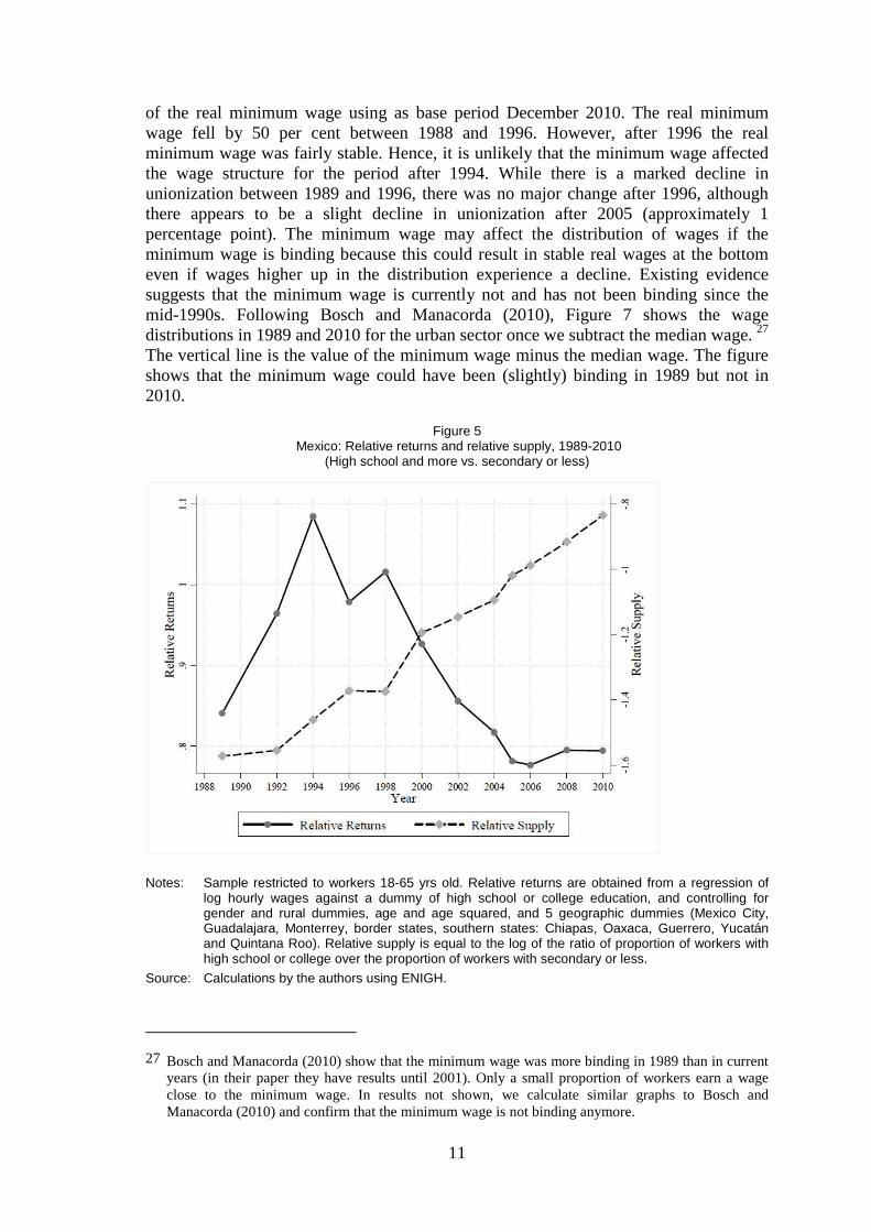
The wage structure (i.e., relative wages by skill, experience, etc.) is affected by demand and supply of workers of different skills (and experience) and by institutional factors such as the minimum wage and unions. Labour demand by skill, in turn, is primarily affected by the characteristics of technical change and international trade. The composition of labour supply is determined, to a large extent, by the characteristics of educational upgrading. Figure 5 plots the relative returns and relative supply of workers with high school education or more against workers with secondary or less. The left y-axis shows the relative returns and the right y-axis the relative supply in logs. The increase in relative supply is larger for the period 1996/98-2010 than for the period 1989-1996/98. The increase in relative supply for the period 1989-98 is approximately 20 per cent while for the period 1998-2010 it is approximately 54 per cent. Inequality measured as the relative returns for workers with at least high school education, on the other hand, increases for the period 1989-94 and it clearly declines for the period 1998-2010.

Following Bound and Johnson (1992), if increases in supply are larger than increases in demand—everything else equal––then we expect relative returns to fall. For the period 1989-94 we observe both an increase in relative supply and a rise in relative returns for workers with tertiary education. Hence, either demand outpaced supply for skilled labour, or institutional factors disfavoured the unskilled, or both. The rapid increase in wage inequality that occurred in Mexico between the mid-1980s and the mid-1990s has been the subject of a fairly large body of research.26 The main conclusions are that institutional factors as well as skill-biased demand explain the observed trend. Further details are discussed in the last section of the paper.

What about the period 1994-2006 when wage inequality declined? In Figure 5 we observe that the relative supply of skilled workers rose while the relative returns declined. This means that either supply outpaced demand, institutional factors moved in favour of the unskilled, or both. Figure 6 shows the evolution of the real minimum wage and the unionization rate for the period 1988-2010. Panel A includes the monthly index

26 The following studies analyse the relevance of institutional factors: Bosch and Manacorda (2010), Fairris (2003) and Fairris, Popli and Zepeda (2008). The relevance of demand factors and skill biased technical change is studied by Airola and Juhn (2005), Bouillon, Legovini and Lustig (2003), Cragg and Epelbaum (1996), Esquivel and Rodríguez-López (2003), Feliciano (2001), Hanson (2003), Hanson and Harrison (1999), López-Acevedo (2006), Meza (2005), Revenga (1997), Robertson (2004, 2007) and Verhoogen (2008).

11

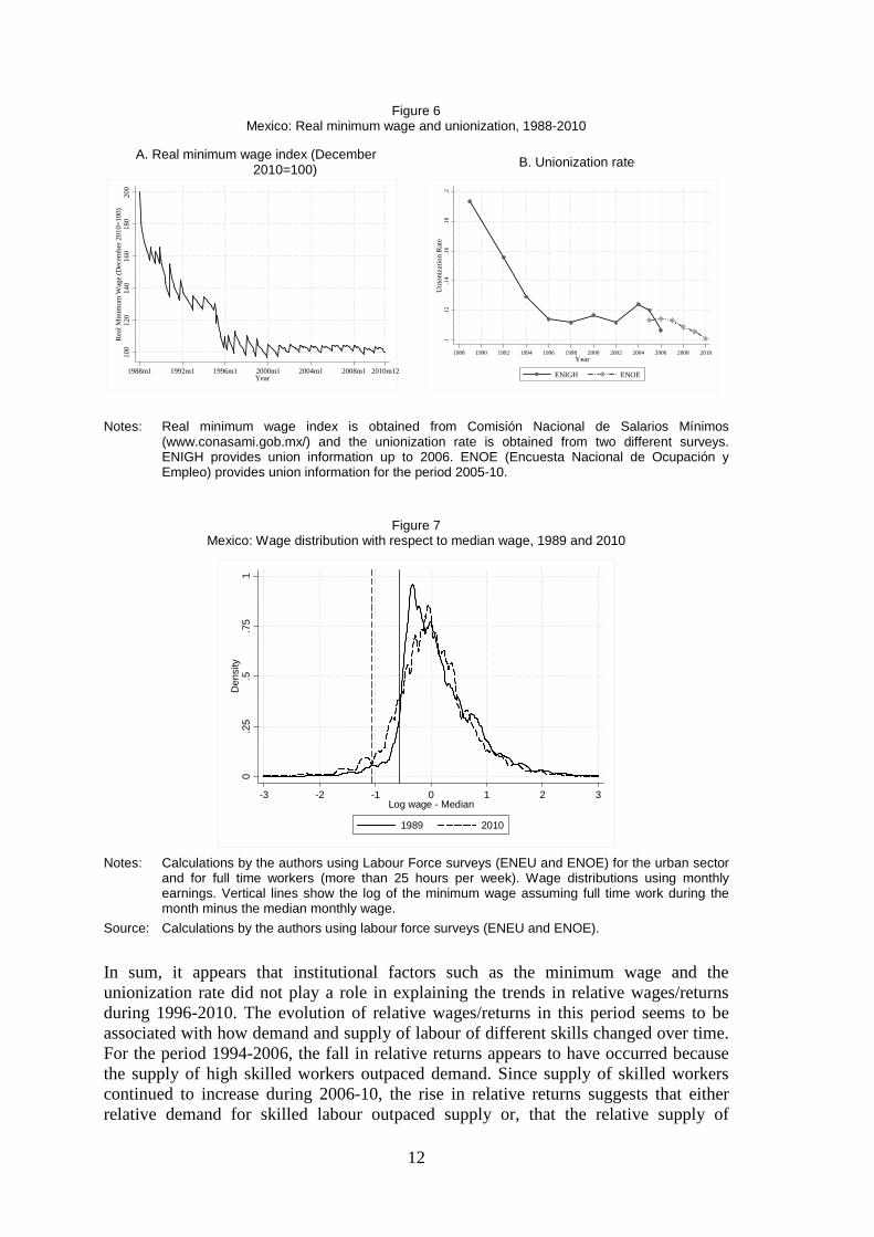
of the real minimum wage using as base period December 2010. The real minimum wage fell by 50 per cent between 1988 and 1996. However, after 1996 the real minimum wage was fairly stable. Hence, it is unlikely that the minimum wage affected the wage structure for the period after 1994. While there is a marked decline in unionization between 1989 and 1996, there was no major change after 1996, although there appears to be a slight decline in unionization after 2005 (approximately 1 percentage point). The minimum wage may affect the distribution of wages if the minimum wage is binding because this could result in stable real wages at the bottom even if wages higher up in the distribution experience a decline. Existing evidence suggests that the minimum wage is currently not and has not been binding since the mid-1990s. Following Bosch and Manacorda (2010), Figure 7 shows the wage distributions in 1989 and 2010 for the urban sector once we subtract the median wage. 27 The vertical line is the value of the minimum wage minus the median wage. The figure shows that the minimum wage could have been (slightly) binding in 1989 but not in 2010.

Figure 5 Mexico: Relative returns and relative supply, 1989-2010

(High school and more vs. secondary or less)

Notes: Sample restricted to workers 18-65 yrs old. Relative returns are obtained from a regression of log hourly wages against a dummy of high school or college education, and controlling for gender and rural dummies, age and age squared, and 5 geographic dummies (Mexico City, Guadalajara, Monterrey, border states, southern states: Chiapas, Oaxaca, Guerrero, Yucatán and Quintana Roo). Relative supply is equal to the log of the ratio of proportion of workers with high school or college over the proportion of workers with secondary or less.

Source: Calculations by the authors using ENIGH.

27 Bosch and Manacorda (2010) show that the minimum wage was more binding in 1989 than in current years (in their paper they have results until 2001). Only a small proportion of workers earn a wage close to the minimum wage. In results not shown, we calculate similar graphs to Bosch and Manacorda (2010) and confirm that the minimum wage is not binding anymore.

12

Figure 6 Mexico: Real minimum wage and unionization, 1988-2010

A. Real minimum wage index (December 2010=100) B. Unionization rate

Notes: Real minimum wage index is obtained from Comisión Nacional de Salarios Mínimos (www.conasami.gob.mx/) and the unionization rate is obtained from two different surveys. ENIGH provides union information up to 2006. ENOE (Encuesta Nacional de Ocupación y Empleo) provides union information for the period 2005-10.

Figure 7 Mexico: Wage distribution with respect to median wage, 1989 and 2010

Notes: Calculations by the authors using Labour Force surveys (ENEU and ENOE) for the urban sector and for full time workers (more than 25 hours per week). Wage distributions using monthly earnings. Vertical lines show the log of the minimum wage assuming full time work during the month minus the median monthly wage.

Source: Calculations by the authors using labour force surveys (ENEU and ENOE).

In sum, it appears that institutional factors such as the minimum wage and the unionization rate did not play a role in explaining the trends in relative wages/returns during 1996-2010. The evolution of relative wages/returns in this period seems to be associated with how demand and supply of labour of different skills changed over time. For the period 1994-2006, the fall in relative returns appears to have occurred because the supply of high skilled workers outpaced demand. Since supply of skilled workers continued to increase during 2006-10, the rise in relative returns suggests that either relative demand for skilled labour outpaced supply or, that the relative supply of

100

120

140

160

180

200

Rea

l Min

imum

Wa

ge (

Dec

embe

r 20

10=

100)

1988m1 1992m1 1996m1 2000m1 2004m1 2008m1 2010m12Year

.1.1

2.1

4.1

6.1

8.2

Uni

oniz

atio

n R

ate

1988 1990 1992 1994 1996 1998 2000 2002 2004 2006 2008 2010Year

ENIGH ENOE

0.2

5.5

.75

1D

ensi

ty

-3 -2 -1 0 1 2 3Log wage - Median

1989 2010

13

unskilled workers outpaced demand.28 We now attempt a more rigorous estimation and account of demand and supply factors

4.1 The effect of demand and supply on relative wages: an application of the Bound and Johnson method (1989-2010)

In order to examine the effect of supply and demand on relative wages, we follow the Bound and Johnson (1992) method.29 Based on the evidence presented in Figures 5 and 6, and as discussed above, we assume that non-competitive factors (i.e., minimum wages and unionization rate) are not important during the 1994-2010 period and ascribe the observed trends in relative wages by skill to demand and supply factors alone.

Assuming a simple CES (constant elasticity of substitution) production function with elasticity of substitution, σ, constant across skills, it is possible to determine the effect of supply and demand on relative wages.30 In particular, it is possible to show that the relative wage of workers with at least high school degree (wC) in terms of the wage of workers with at most secondary education (wS) can be expressed in terms of its increase in demand and supply:

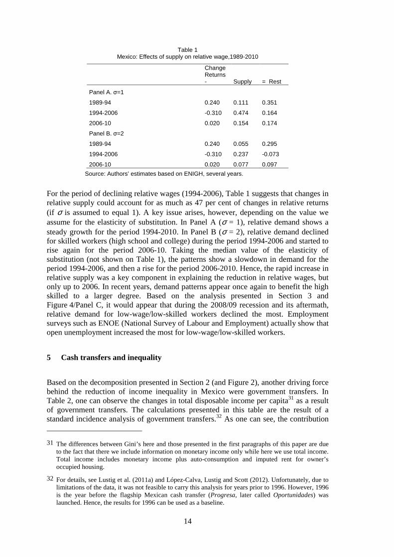
The residual term contains the effect of skill-biased technical change and other non-competitive factors. As the unionization rate and the real minimum wage were fairly constant during 1994-2006, we assume non-competitive factors are negligible. In order to make the simulation simpler, we only simulate changes in supply and assign the full residual to demand and skill-biased technical change (which affects demand, of course). The supply component is equal to the relative increase of workers with at least high school education divided by workers with at most secondary education. Table 1 shows the results of the simulation assuming an elasticity of substitution of 1 and 2 which is the consensus in the literature (Bound and Johnson 1992; Katz and Autor 1999).

Consistent with previous research findings, Table 1 suggests that changes in relative supply had a small effect on relative wages in the period between 1989 and 1994. Most of the changes for that period, then, have to be explained by changes in demand and institutional factors, as discussed above. The relative contribution of market versus institutional factors, however, cannot be cleanly disentangled.

28 Using ENOE for the period 2006-2010, we find that the relative returns of college educated workers against workers with primary or less declined 0.01 points. However the decline in returns was larger for high school educated workers and workers with secondary. Hence, the result of the slowdown in returns for college educated workers is robust to the selection of the microdata: ENIGH and ENOE.

29 We attempted to estimate a model similar to Bound and Johnson (1992) and Manacorda et.al. (2010). However, as pointed out by Manacorda et al. (2010), the relevant elasticities of substitution for the case of Mexico cannot be precisely estimated. In order to estimate the structural parameter σ, Manacorda et al. (2010) use a sample of workers from Argentina, Brazil, Chile, Colombia and Mexico; they mention that ‘Mexico does not really contribute to the identification of the regression parameters’ (footnote 1, page 314).

30 See formula (3) in page 377 and formula (A8) in page 390 of Bound and Johnson (1992).

( ) ξσσ

+∆−∆

∆ SupplyDemand

w

wS

C

%1

)%(1

=%

ξ

14

Table 1 Mexico: Effects of supply on relative wage,1989-2010

Change Returns - Supply = Rest

Panel A. σ=1

1989-94 0.240 0.111 0.351

1994-2006 -0.310 0.474 0.164

2006-10 0.020 0.154 0.174

Panel B. σ=2

1989-94 0.240 0.055 0.295

1994-2006 -0.310 0.237 -0.073

2006-10 0.020 0.077 0.097

Source: Authors’ estimates based on ENIGH, several years.

For the period of declining relative wages (1994-2006), Table 1 suggests that changes in relative supply could account for as much as 47 per cent of changes in relative returns (if σ is assumed to equal 1). A key issue arises, however, depending on the value we assume for the elasticity of substitution. In Panel A (σ = 1), relative demand shows a steady growth for the period 1994-2010. In Panel B (σ = 2), relative demand declined for skilled workers (high school and college) during the period 1994-2006 and started to rise again for the period 2006-10. Taking the median value of the elasticity of substitution (not shown on Table 1), the patterns show a slowdown in demand for the period 1994-2006, and then a rise for the period 2006-2010. Hence, the rapid increase in relative supply was a key component in explaining the reduction in relative wages, but only up to 2006. In recent years, demand patterns appear once again to benefit the high skilled to a larger degree. Based on the analysis presented in Section 3 and Figure 4/Panel C, it would appear that during the 2008/09 recession and its aftermath, relative demand for low-wage/low-skilled workers declined the most. Employment surveys such as ENOE (National Survey of Labour and Employment) actually show that open unemployment increased the most for low-wage/low-skilled workers.

5 Cash transfers and inequality

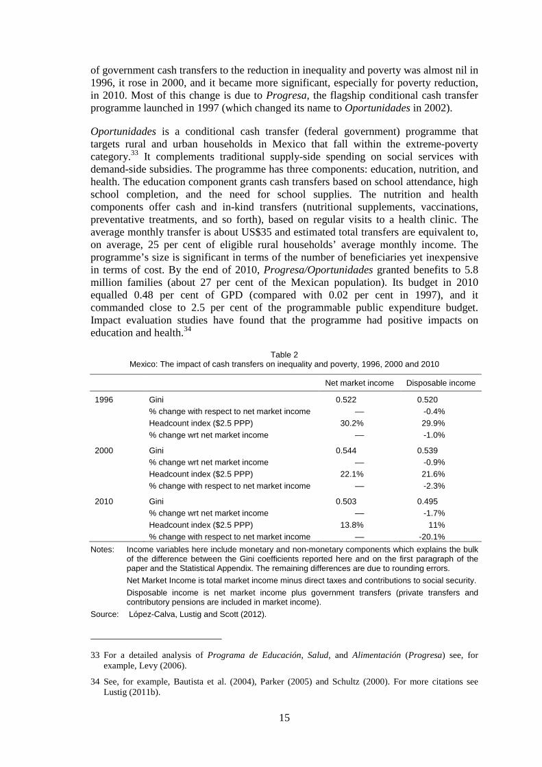
Based on the decomposition presented in Section 2 (and Figure 2), another driving force behind the reduction of income inequality in Mexico were government transfers. In Table 2, one can observe the changes in total disposable income per capita31 as a result of government transfers. The calculations presented in this table are the result of a standard incidence analysis of government transfers.32 As one can see, the contribution

31 The differences between Gini’s here and those presented in the first paragraphs of this paper are due to the fact that there we include information on monetary income only while here we use total income. Total income includes monetary income plus auto-consumption and imputed rent for owner’s occupied housing.

32 For details, see Lustig et al. (2011a) and López-Calva, Lustig and Scott (2012). Unfortunately, due to limitations of the data, it was not feasible to carry this analysis for years prior to 1996. However, 1996 is the year before the flagship Mexican cash transfer (Progresa, later called Oportunidades) was launched. Hence, the results for 1996 can be used as a baseline.

15

of government cash transfers to the reduction in inequality and poverty was almost nil in 1996, it rose in 2000, and it became more significant, especially for poverty reduction, in 2010. Most of this change is due to Progresa, the flagship conditional cash transfer programme launched in 1997 (which changed its name to Oportunidades in 2002).

Oportunidades is a conditional cash transfer (federal government) programme that targets rural and urban households in Mexico that fall within the extreme-poverty category.33 It complements traditional supply-side spending on social services with demand-side subsidies. The programme has three components: education, nutrition, and health. The education component grants cash transfers based on school attendance, high school completion, and the need for school supplies. The nutrition and health components offer cash and in-kind transfers (nutritional supplements, vaccinations, preventative treatments, and so forth), based on regular visits to a health clinic. The average monthly transfer is about US$35 and estimated total transfers are equivalent to, on average, 25 per cent of eligible rural households’ average monthly income. The programme’s size is significant in terms of the number of beneficiaries yet inexpensive in terms of cost. By the end of 2010, Progresa/Oportunidades granted benefits to 5.8 million families (about 27 per cent of the Mexican population). Its budget in 2010 equalled 0.48 per cent of GPD (compared with 0.02 per cent in 1997), and it commanded close to 2.5 per cent of the programmable public expenditure budget. Impact evaluation studies have found that the programme had positive impacts on education and health.34

Table 2 Mexico: The impact of cash transfers on inequality and poverty, 1996, 2000 and 2010

Net market income Disposable income 1996 Gini 0.522 0.520

% change with respect to net market income –– -0.4% Headcount index ($2.5 PPP) 30.2% 29.9% % change wrt net market income –– -1.0%

2000 Gini 0.544 0.539

% change wrt net market income –– -0.9% Headcount index ($2.5 PPP) 22.1% 21.6% % change with respect to net market income –– -2.3%

2010 Gini 0.503 0.495

% change wrt net market income –– -1.7% Headcount index ($2.5 PPP) 13.8% 11% % change with respect to net market income –– -20.1%

Notes: Income variables here include monetary and non-monetary components which explains the bulk of the difference between the Gini coefficients reported here and on the first paragraph of the paper and the Statistical Appendix. The remaining differences are due to rounding errors.

Net Market Income is total market income minus direct taxes and contributions to social security.

Disposable income is net market income plus government transfers (private transfers and contributory pensions are included in market income).

Source: López-Calva, Lustig and Scott (2012).

33 For a detailed analysis of Programa de Educación, Salud, and Alimentación (Progresa) see, for example, Levy (2006).

34 See, for example, Bautista et al. (2004), Parker (2005) and Schultz (2000). For more citations see Lustig (2011b).

16

All in all, Progresa/Oportunidades transformed the broadly neutral distribution of government spending on food subsidies into a highly progressive one: the share benefiting the poorest decile increased from 8 to 33 per cent between 1994 and 2000.35

Beyond its effects on education, health, and nutrition, Progresa/Oportunidades has had a positive impact on poor households’ consumption, thereby helping to reduce poverty and inequality in Mexico. In 2004, poverty incidence among programme participants (the percentage of the population associated with the program that is below the poverty line) fell by 9.7 per cent in rural areas and by 2.6 per cent in urban areas.36 In terms of its impact on the distribution of income, the direct effect of Progresa/Oportunidades transfers was equivalent to close to one-fifth of the decline in the Gini coefficient between 1996 and 2006.37

6 Concluding remarks: the rise and fall of income inequality and policy regimes

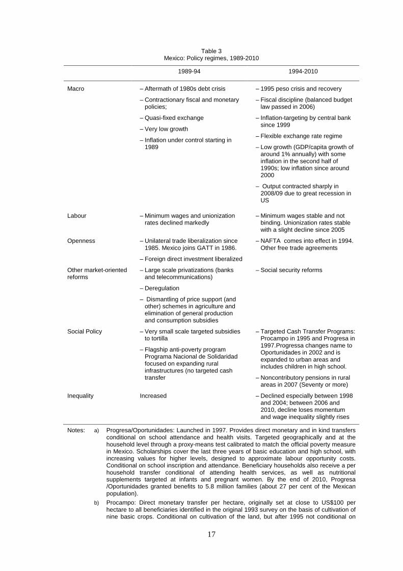
Previously we identified three episodes in inequality dynamics in Mexico: a period of rising inequality (1989-94); a period of declining inequality (1994-2006); and a period in which the decline in inequality lost its momentum (2006-10). These periods coincide with, roughly, two broad policy regimes. (Table 3) Between 1989 and 1994, the policy regime was characterized by intense and widespread market-oriented reforms (with trade liberalization and privatizations taking the lead), dismantling of price supports and generalized subsidies, and reductions in the minimum wages and unionization rates. After 1994, the policy regime was characterized by a paucity in structural reforms, strategic integration with the rest of the world (of which the salient example is the North American Free Trade Agreement or NAFTA), and the introduction of large-scale (in terms of beneficiaries) cash transfer programmes. Minimum wages became non-binding and the unionization rate remained low. What, if any, might be the connection between the policy regimes and inequality outcomes?

Our analysis indicates that the rise in overall inequality between 1989 and 1994 is accounted for, to a large extent, by the rise in labour income inequality. The rise in labour income inequality, in turn, is associated with the increase in relative returns for skilled workers (where skilled workers are those who hold a high school degree or more). The increase in the skilled-unskilled wage gap coincided with the unilateral trade liberalization that started in the mid-1980s (Table 3). In that sense, the evolution of Mexico’s wage inequality was unexpected; Mexico had an abundance of relatively unskilled labour (at least from the perspective of its main trade partner, the United States), and standard theories of trade predicted exactly the opposite pattern (that is, a reduction in the skilled-unskilled wage ratio).38

35 See Scott (2009).

36 Cortés, Solís and Banegas (2006).

37 Scott (2009). The impact on the Gini coefficient takes account of only the direct effect. The effects on inequality of changes in behavior or of higher human capital among the poor are not contemplated in this calculation.

38 For a discussion of trade liberalization and its implications see, for example, Lustig (1998).

17

Table 3 Mexico: Policy regimes, 1989-2010

1989-94 1994-2010

Macro

– Aftermath of 1980s debt crisis

– Contractionary fiscal and monetary policies;

– Quasi-fixed exchange

– Very low growth

– Inflation under control starting in 1989

– 1995 peso crisis and recovery

– Fiscal discipline (balanced budget law passed in 2006)

– Inflation-targeting by central bank since 1999

– Flexible exchange rate regime

– Low growth (GDP/capita growth of around 1% annually) with some inflation in the second half of 1990s; low inflation since around 2000

– Output contracted sharply in 2008/09 due to great recession in US

Labour – Minimum wages and unionization rates declined markedly

– Minimum wages stable and not binding. Unionization rates stable with a slight decline since 2005

Openness – Unilateral trade liberalization since 1985. Mexico joins GATT in 1986.

– Foreign direct investment liberalized

– NAFTA comes into effect in 1994. Other free trade agreements

Other market-oriented reforms

– Large scale privatizations (banks and telecommunications)

– Deregulation

– Dismantling of price support (and other) schemes in agriculture and elimination of general production and consumption subsidies

– Social security reforms

Social Policy – Very small scale targeted subsidies to tortilla

– Flagship anti-poverty program Programa Nacional de Solidaridad focused on expanding rural infrastructures (no targeted cash transfer

– Targeted Cash Transfer Programs: Procampo in 1995 and Progresa in 1997.Progressa changes name to Oportunidades in 2002 and is expanded to urban areas and includes children in high school.

– Noncontributory pensions in rural areas in 2007 (Seventy or more)

Inequality Increased – Declined especially between 1998 and 2004; between 2006 and 2010, decline loses momentum and wage inequality slightly rises

Notes: a) Progresa/Oportunidades: Launched in 1997. Provides direct monetary and in kind transfers conditional on school attendance and health visits. Targeted geographically and at the household level through a proxy-means test calibrated to match the official poverty measure in Mexico. Scholarships cover the last three years of basic education and high school, with increasing values for higher levels, designed to approximate labour opportunity costs. Conditional on school inscription and attendance. Beneficiary households also receive a per household transfer conditional of attending health services, as well as nutritional supplements targeted at infants and pregnant women. By the end of 2010, Progresa /Oportunidades granted benefits to 5.8 million families (about 27 per cent of the Mexican population).

b) Procampo: Direct monetary transfer per hectare, originally set at close to US$100 per hectare to all beneficiaries identified in the original 1993 survey on the basis of cultivation of nine basic crops. Conditional on cultivation of the land, but after 1995 not conditional on

18

particular crops. Administrative data: 2.39 million beneficiaries in 2008.

c) Seventy or more: Non-contributory pension. All the population of 70 years and older living in localities of 30,000 or less are eligible for this universal rural non-contributory basic pension of 500 pesos (US$37) per month. Administrative data: 1.031 million beneficiaries in 2008.

Source: Authors’ compilation based on Lustig (2010).

Why did trends in relative wages during 1989 and 1994 contradict expectations (stemming from standard trade theory)? First, this period also coincided with labour market policies/institutional changes that disfavoured the low-skilled: a reduction in real minimum wages and in the unionization rate (Table 3 and Figure 6). Bosch and Manacorda (2010) find evidence that these institutional factors were quite decisive in causing wage inequality to rise. In addition, there is evidence that the direct and indirect impact of the opening up of the economy (trade liberalization and foreign direct investment liberalization) contributed to the rise in the wage gap by skill. The direct effect occurred because—contrary to expectations-- some labour-intensive sectors (such as textiles and garments) were relatively more protected under import-substitution industrialization and were hurt by trade liberalization.39 The indirect effect manifested itself through skill-biased technical change (though, admittedly, it is hard to disentangle which part of the latter is induced by openness or occurs independently).

Is there a connection between the policies pursued after 1994 and the decline in overall inequality? Again, the results of the decomposition exercise presented in Section 2 and in Esquivel, Lustig and Scott suggest that one of the most important inequality-reducing forces between 1994 and 2006 has been the evolution of labour income inequality. Note that labour income is basically the result of multiplying hours worked by hourly wages (here defined as including remunerations to the self-employed). It turns out that hours worked did not change much from 1994 to 2006,40 so the change in labour income inequality must have been caused by changes in hourly wage inequality. Some authors have linked the reduction in wage inequality to NAFTA. Robertson (2007), for example, suggests that Mexico’s manufacturing workers are now complements, rather than substitutes, to US workers. He also posits that there has been an important expansion of assembly-line activities in Mexico (maquiladoras), which has increased demand for less-skilled workers.41 Campos (2008) emphasizes the supply-side explanations based on changes in the composition of the labour force.

39 See, for example, Hanson and Harrison (1999) and Revenga (1997).

40 Actually, between 1994 and 2006, weekly hours in all jobs fell slightly and the decline was concentrated in low education (poorer) workers which would be an inequality-increasing change. This means that the inequality-reducing changes in the distribution of hourly earnings must have been large enough to compensate for the inequality-increasing effect of the changes in the distribution of hours worked. Data on weekly hours and hourly wages are available at: www.depeco.econo .unlp.edu.ar/sedlac/.

41 Robertson (2007) notices that the pattern of wage inequality in Mexico is puzzling because no single theory could explain the evolution of wage inequality before and after NAFTA. There are, however, some tentative theoretical explanations for the pattern. For example, Atolia (2007) has suggested that, under certain circumstances, even if the standard prediction from a Hecksher-Ohlin-Samuelson model works as predicted in the long-run, there may be some short-run (or transitory) effects of trade liberalization that may lead to a different outcome from those of the long-run. The difference between short-run and long-run effects on inequality result from two factors: first, an asymmetry in the contraction and expansion of some sectors, and second, because of the capital-skill complementarity in production.

19

Between 1989 and 1994, most of the changes in the wage distribution occurred in the upper tail of the distribution (workers with high wages and high levels of education and experience). As was seen in Figure 4, Panel A, the increase in wage inequality in those years was not caused by a (relative) decline in the wages of the low-skilled or low-experienced workers; rather it was the result of a higher rise in the wages of the high-skilled or high-experienced workers. In contrast, between 1994 and 2006 the reduction in wage inequality was caused by the changes in the lower tail of the income distribution. Average wages for workers with lower levels of education and/or fewer years of experience increased (Figure 4, Panel B), even though average real and legislated minimum wages were practically flat over this period (Figure 6). Average wages for higher-paid workers (high-skilled and/or high-experienced workers), in contrast, declined between 1994 and 2006 (Figure 4, Panel B).

For the post-NAFTA period (after 1994), then, there are at least two (not mutually exclusive) possible explanations: an increase in the relative supply of skilled workers and an increase in the demand for low-skilled labour resulting from an expansion in assembly-line activities (maquiladoras) in Mexico’s manufacturing sector.42 Based on our analysis presented in Section 4 (Table 1), the reduction in relative returns of the high-skilled workers seems to be driven, primarily, by the rise in their relative supply.

The increase in the relative supply of workers with high levels of skills reflects the significant educational upgrading of the labour force that occurred during this period. (Figure 5) Part of this upgrading should be the consequence of the expansionary policies in terms of access to education (see Esquivel, Lustig and Scott). However, part might also be a consequence of more individuals deciding to invest in a tertiary degree in response to the rising returns to skill experienced between 1989 and 1994 (and, actually since 1984). This would suggest that Mexico experienced a Tinbergean process in the sense that skill-biased demand (due to trade liberalization and technical change) contributed (along with institutional factors) to a significant increase in the skill premium. This, in turn, could have induced individuals to invest more in their own education (completing high school and tertiary degrees). The subsequent increase in the relative supply of more educated workers (high school and more) caused the skill premium (and wage inequality) to decline.

In sum, the results reveal the following. Relative supply only marginally affected the wage structure during the period 1989-94. Therefore, relative demand and institutional factors are responsible for the increase in inequality. On the other hand, after 1994 institutional factors have remained largely unchanged; in particular, the minimum wage became non-binding during the period. At the same time, relative supply of skilled labour (completed high school or more) increased by more than 50 per cent and relative demand slowed down which resulted in lower inequality. The period 2006-2010 has seen a small increase in inequality. This is mainly due to a decrease in wages at the bottom and not to an increase of wages at the top. Does this point to a reversal in the wage inequality dynamics in Mexico? At this point, it is too soon to be able to disentangle the permanent versus the temporal effects of the recent macroeconomic crisis caused by the Great Recession in the United States.

42 Campos (2008); Robertson (2007).

20

Finally, overall inequality has declined because non-labour income inequality declined too. Our analysis and that presented in Esquivel, Lustig and Scott suggest that a change in social policy from general subsidies to cash transfers targeted to the poor contributed to the decline in inequality especially since 2000, when the number of beneficiaries was increased.

References

Airola, J., and C. Juhn (2005). ‘Wage Inequality in Post-Reform Mexico’. IZA Discussion Papers 1525. Bonn: Institute for the Study of Labour (IZA).

Almeida dos Reis, J., and R. Paes de Barros (1991). ‘Wage Inequality and the Distribution of Education: A Study of the Evolution of Regional Differences in Inequality in Metropolitan Brazil’. Journal of Development Economics, 36(1): 117–43.

Atolia, Manoj (2007). “Trade Liberalization and Rising Wage Inequality in Latin America: Reconciliation with HOS Theory,” Journal of International Economics, April.

Autor, D. H., L. F. Katz, and M. S. Kearney (2008). ‘Trends in U.S. Wage Inequality Revising the Revisionists’. The Review of Economics and Statistics, 90(2): 290–9.

Bautista, S., S. Bertozzi, P. Gertler, J. P. Guiterrez, and M. Hernández (2004). The Impact of Oportundades on Health Status, Morbidity, and Service Utilization among Beneficiary Population: Short-term Results in Urban Areas and Medium-term Results in Rural Areas. Cuernavaca, Mexico: National Institute of Public Health.

Bosch, M., and M. Manacorda (2010). ‘Minimum Wages and Earnings Inequality in Urban Mexico’. American Economic Journal: Applied Microeconomics, 2(4): 128-–49.

Bouillón, C., A. Legovini, and N. Lustig (2003). ‘Rising Inequality in Mexico: Household Characteristics and Regional Effects’. Journal of Development Studies, 39(4): 112-–33.

Bound, J., and G. Johnson (1992). ‘Changes in the Structure of Wages in the 1980s: An Evaluation of Alternative Explanations’. The American Economic Review, 82(3): 371–92.

Bourguignon, F., F. Ferreira, and N. Lustig (2005). The Microeconomics of Income Distribution Dynamics in East Asia and Latin America. Washington, DC: Oxford University Press, Washington.

Campos, R. (2008). ‘Why did Wage Inequality Decrease in Mexico after NAFTA?’. Berkeley: University of California at Berkeley (October). Mimeo.

Card, D., and J. DiNardo (2002). ‘Skill Biased Technological Change and Rising Wage Inequality: Some Problems and Puzzles’. Journal of Labour Economics, 20(4): 733–83.

21

Chernozhukov, V., I. Fernandez-Val, and B. Melly (2009). ‘Inference on Counterfactual Distributions’. CeMMAP Working Papers CWP09/09. London: Centre for Microdata Methods and Practice, Institute for Fiscal Studies.

Chi, W., B. Li, and Q. Yu (2011). ‘Decomposition of the Increase in Earnings Inequality in Urban China: A Distributional Approach’. China Economic Review, 22(3): 299-312.

Cortés, F., P. Solís, and I. Banegas (2006). ‘Oportunidades y Pobreza en Mexico: 2002-2004’. Working Paper. Mexico City: Secretaria de Hacienda y Crédito Público.

Cragg, M., and M. Epelbaum (1996). ‘Why has Wage Dispersion Grown in Mexico? Is it the Incidence of Reforms or the Growing Demand for Skills?’. Journal of Development Economics, 51(1): 99-116.

DiNardo, J., N. M. Fortin, and T. Lemieux (1996). ‘Labour Market Institutions and the Distribution of Wages, 1973-1992: A Semiparametric Approach’. Econometrica, 64 (5): 1001-44.

Esquivel, G. (2011). ‘The Dynamics of Income Inequality in Mexico since NAFTA’. Economia, 12(1): 155–79.

Esquivel, G., N. Lustig, and J. Scott (2010). ‘Mexico: A Decade of Falling Inequality: Market Forces or State Action?’ In L. F. López and N. Lustig (eds), Declining Inequality in Latin America: A Decade of Progress? Washington, DC: Brookings Institution Press and New York: United Nations Development Programme.

Esquivel, G., and J. A. Rodríguez-López (2003). ‘Technology, Trade and Wage Inequality’. Journal of Development Economics, 72(2): 543-–65.

Fairris, D. (2003). ‘Unions and Wage Inequality in Mexico’. Industrial and Labour Relations Review, 56(3): 481–97.

Fairris, D., G. Popli, and E. Zepeda (2008). ‘Minimum Wages and the Wage Structure in Mexico’. Review of Social Economy, 66(2): 181-208.

Feliciano, Z. (2001). ‘Workers and Trade Liberalization. The Impact of Trade Reform. The case of Mexico’. Industrial and Labour Relations Review, 55(1): 95–115.

Firpo, S., N. Fortin, and T. Lemieux (2009). ‘Unconditional Quantile Regressions’. Econometrica, 77(3): 953–73.

Firpo, S., N. Fortin, and T. Lemieux (2011). ‘Decomposition Methods in Economics’. In. D. Card and O. Ashenfelter (eds), Handbook of Labour Economics. Amsterdam: North Holland, 2–104.

Gasparini, L., S. Galiani, G. Cruces, and P. Acosta (2011). ‘Educational Upgrading and Returns to Skills in Latin America. Evidence from a Supply-Demand Framework.’ WB Policy Research Working Paper 5921. Washington, DC: World Bank.

Hanson, G. (2003). ‘What has Happened to Wages in Mexico since NAFTA? Implications for Hemispheric Free Trade’. NBER Working Paper 9563. Cambridge, MA: National Bureau of Economic Research.

Hanson, G., and H. Harrison (1999). ‘Trade Liberalization and Wage Inequality’. Industrial and Labour Relations Review, 52(2): 271–88.

22

Hernández, B. and others (2003). ‘Evaluación del Impact de Oportunidades en la Mortalidad Materna e Infantil.’ In B. Hernández Prado and M. Hernández Avila (eds), Evaluación del Impacto del Programa Oportunidades, vol. 2. Cuernavaca, Mexico: Instituto Nacional de Salud Pública.

Holmes, C., and K. Mayhew (2010). ‘Are UK Labour Markets Polarising?’. Research Paper 97. Oxford: ERSC Centre on Skills, Knowledge and Organisational Performance (SKOPE).

Jann, B. (2008). ‘A Stata Implementation of the Blinder-Oaxaca Decomposition’. Stata Journal, 8(4): 453–79.

Juhn, C., K. Murphy, and B. Pierce (1993). ‘Wage Inequality and the Rise in Returns to Skill’. Journal of Political Economy, 3(3): 410–48.

Katz, L. F., and D. H. Autor (1999). ‘Changes in the Wage Structure and Earnings Inequality’. In O. Ashenfelter and D. Card (eds), Handbook of Labour Economics, vol. 3. Amsterdam: North Holland.

Legovini, A., C. Bouillon, and N. Lustig (2005). ‘Can Education Explain Changes in Income Inequality in Mexico’. In F. Bourguignon, F. H. G. Fereira and N. Lustig (eds), The Microeconomics of Income Distribution Dynamics. Washington, DC: Oxford University Press for the World Bank, 275–312.

Lerman, R. I., and S. Yitzhaki (1985). ‘Income Inequality Effects by Income Source: A New Approach and Applications to the United States’. Review of Economics and Statistics, 67: 151–6.

Levy, S. (2006). Progress against Poverty. Washington, DC: Brookings Institution Press.

López-Acevedo, G. (2006). ‘Mexico: Two Decades of the Evolution of Education and Inequality’. WB Policy Research Working Paper 3919. Washington, DC: World Bank.

López-Calva, L. F., N. Lustig, and J. Scott (2012). ‘Government Transfers and Redistribution in Mexico: 1996-2010’. Work in progress. Washington, DC: World Bank.

Lustig, N. (1998). Mexico: The Remaking of an Economy (2nd ed.). Washington, DC: The Brookings Institution.

Lustig, N. (2010). ‘El impacto de 25 años de reformas sobre la pobreza y la desigualdad’. In N. Lustig (ed.), Crecimiento económico y equidad. Mexico City: El Colegio de México.

Lustig, N., and others (coordinator) (2011a). ‘Fiscal Policy and Income Redistribution in Latin America: Challenging the Conventional Wisdom’. Background paper for Corporacion Andina de Fomento (CAF) Fiscal Policy for Development: Improving the Nexus between Revenues and Spending (Política Fiscal para el Desarrollo: Mejorando la Conexión entre Ingresos y Gastos.

Lustig, N. (2011b). ‘Scholars who became Practitioners: The Influence of Research on the Design, Evaluation and Political Survival of Mexico’s Anti-Poverty Program Progresa/Oportunidades’. Tulane Economics Department Working Paper 1123. New Orleans: Tulane University.

23

Machado, J. A. F., and J. Mata (2005). ‘Counterfactual Decomposition of Changes in Wage Distributions using Quantile Regression’. Journal of Applied Econometrics, 20(4): 445–65.

Manacorda, M., C. Sánchez-Páramo, and N. Schady (2010). ‘Changes in Returns to Education in Latin America: The Role of Demand and Supply of Skills’. Industrial and Labour Relations Review, 63(2): 307–26.

Meza, L. G. (2005). ‘Mercados Laborales Locales y Desigualdad Salarial en México’. El Trimestre Económico, 72(1), 133–78.

Parker, S. (2005). ‘Evaluación del Impacto de Oportunidades sobre la Inscripción, Reprobación, y Abandono Escolar’. In B. Hernández Prado and M. Hernández Avila (eds), Evaluación Externa del Impacto del Programa Oportunidades. Mexico: Instituto Nacional de Salud Pública.

Revenga, A. (1997). ‘Employment and Wage Effects of Trade Liberalization: The Case of Mexican Manufacturing’. Journal of Labour Economics, 15(3): 20–43.

Robertson, R. (2004). ‘Relative Prices and Wage Inequality. Evidence from Mexico’. Journal of International Economics, 64(2): 387–409.

Robertson, R. (2007). ‘Trade and Wages: Two Puzzles from Mexico’. The World Economy, 30(9): 1378–98.

Schultz, P. (2000). The Impact of Progresa on School Enrollments: Final Report. Washington, DC: International Food Policy Research Institute.

Scott, J. (2009). ‘Redistributive Constraints under High Inequality: The Case of Mexico’. Paper prepared for the UNDP project ‘Markets, the State, and the Dynamics of Inequality: How to Advance Inclusive Growth’.

Stark, O., J. E. Taylor, and S. Yitzhaki (1986). ‘Remittances and inequality’. Economic Journal, 96: 722–740.

Thu Le, H., and A. L. Booth (2010). ‘Inequality in Vietnamese Urban-Rural Living Standards, 1993-2006. IZA Discussion Paper 4987. Bonn: Institute for the Study of Labour.

Verhoogen, E. (2008). ‘Trade, Quality Upgrading, and Wage Inequality in the Mexican Manufacturing Sector’. Quarterly Journal of Economics, 123(2): 489–530.

24

Acronyms

ENIGH Encuesta Nacional de Ingresos y Gastos de los Hogares (National Survey of Household Incomes and Expenditures)

ENOE National Survey of Labour and Employment

GATT General Agreement of Tariffs and Trade

NAFTA North American Free Trade Agreement

OB Oaxaca-Blinder type of decomposition

RIF re-centred influence function

SEDLAC Socioeconomic Database for Latin America and the Caribbean

Methodological appendix

Static decomposition of the Gini coefficient: Lerman and Yitzhaki method

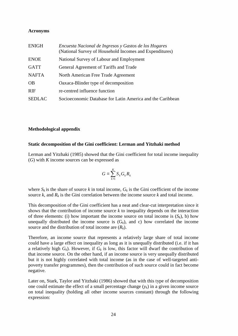
Lerman and Yitzhaki (1985) showed that the Gini coefficient for total income inequality (G) with K income sources can be expressed as

where Sk is the share of source k in total income, Gk is the Gini coefficient of the income source k, and Rk is the Gini correlation between the income source k and total income.

This decomposition of the Gini coefficient has a neat and clear-cut interpretation since it shows that the contribution of income source k to inequality depends on the interaction of three elements: (i) how important the income source on total income is (Sk), b) how unequally distributed the income source is (Gk), and c) how correlated the income source and the distribution of total income are (Rk).

Therefore, an income source that represents a relatively large share of total income could have a large effect on inequality as long as it is unequally distributed (i.e. if it has a relatively high Gk). However, if Gk is low, this factor will dwarf the contribution of that income source. On the other hand, if an income source is very unequally distributed but it is not highly correlated with total income (as in the case of well-targeted anti-poverty transfer programmes), then the contribution of such source could in fact become negative.

Later on, Stark, Taylor and Yitzhaki (1986) showed that with this type of decomposition one could estimate the effect of a small percentage change (yk) in a given income source on total inequality (holding all other income sources constant) through the following expression:

∑=

=K

kkkk RGSG

1

25

�����

������� � ��

or, alternatively,

�����

�

������

�� ��

This expression means that the per cent change in inequality resulting from a marginal percentage change in income source k is equal to the initial share of income source k on total income inequality minus the initial share of the income source k.