the role of location in evaluating racial wage...

Electronic copy available at: http://ssrn.com/abstract=1468435

Research Division Federal Reserve Bank of St. Louis Working Paper Series

The Role of Location in Evaluating Racial Wage Disparity

Dan A. Black Natalia Kolesnikova

Seth G. Sanders and

Lowell J. Taylor

Working Paper 2009-043A

http://research.stlouisfed.org/wp/2009/2009-043.pdf

September 2009

FEDERAL RESERVE BANK OF ST. LOUIS Research Division

P.O. Box 442 St. Louis, MO 63166

______________________________________________________________________________________

The views expressed are those of the individual authors and do not necessarily reflect official positions of the Federal Reserve Bank of St. Louis, the Federal Reserve System, or the Board of Governors.

Federal Reserve Bank of St. Louis Working Papers are preliminary materials circulated to stimulate discussion and critical comment. References in publications to Federal Reserve Bank of St. Louis Working Papers (other than an acknowledgment that the writer has had access to unpublished material) should be cleared with the author or authors.

Electronic copy available at: http://ssrn.com/abstract=1468435

THE ROLE OF LOCATION INEVALUATING RACIAL WAGE DISPARITY

(WORK IN PROGRESS)

DAN A. BLACK, NATALIA KOLESNIKOVA, SETH G. SANDERS, AND LOWELL J. TAYLOR

Abstract. A standard object of empirical analysis in labor economics is a modified Mincer

wage function in which an individual’s log wage is specified to be a function of education,

experience, and an indicator variable identifying race. Researchers hope that estimates from

this exercise can be informative about the impact of minority status on labor market success.

Here we set out a theoretical justification for this regression in a context in which individuals

live and work in different locations. Our model leads to the traditional approach, but with

the important caveat that the regression should include location-specific fixed effects. Given

this insight, we reevaluate evidence about the black-white wage disparity in the United

States.

JEL: J31, J71, R23.

Keywords: wage regressions, racial wage disparity, theory of local labor markets.

Introduction

In hundreds of studies social scientists have examined the role of minority status in wage

determination by estimating variants of the Mincer earnings function,

(1) ln(wi) = β1Ri + β2Ei + γ(Xi) + εi;

where the expected log wage of individual i is specified to be a function of an indicator vari-

able for minority demographic status Ri (e.g., race, immigrant status, ethnicity, or gender),

education Ei (or an alternative measure of human capital), and also, typically, some function

of such covariates as age or experience, given by γ(Xi). A statistically significant estimated

Date: August 2009. Author affiliations: Black, University of Chicago and NORC; Kolesnikova, Federal

Reserve Bank of St. Louis; Sanders, Duke University; and Taylor, Carnegie Mellon University. The views

expressed are ours and do not necessarily reflect official positions of the Federal Reserve Bank of St. Louis,

the Federal Reserve System, or the Board of Governors. Helpful comments on earlier drafts were provided

by David Card, Enrico Moretti, and seminar participants at UC Berkeley.1

2 DAN A. BLACK, NATALIA KOLESNIKOVA, SETH G. SANDERS, AND LOWELL J. TAYLOR

negative value of β1 is taken as an indication of wage disparity that adversely affects mi-

nority workers—disparity that arises from disparate treatment in the labor market, or from

differences in human capital that are correlated with minority status.

Here we study the properties of the estimates of regression (1) when individuals live in

locations that have differing prices, e.g., different local wages, housing prices, and prices of

other goods and services.1 We are interested in both of the possibilities mentioned above—

that wage gaps are due to discrimination or due to unmeasured differences in human capital.

Either way, we find that in a standard model of local labor markets, β1 is a single parameter

only under fairly restricted conditions, and even then can be estimated consistently only if

one include location fixed effects into equation (1).

With this observation in mind, we turn to two empirical exercises. First, we conduct an

analysis of black-white wage gaps in the United States from 1940 through 2000—work that

roughly parallels the well-known work of Smith and Welch (1989). Second, we conduct an

analysis of black-white wage gaps, as well as wage gaps between Hispanics and non-Hispanic

whites, in which we control for cognitive test scores (AFQT scores), as in Neal and Johnson’s

(1996) important paper. In both cases, we discover that an empirical approach that accounts

for location yields results that differ substantially from approaches that implicitly ignore

location.

Our paper proceeds in four additional sections:

The first section sets out a standard model of urban differences in prices, and in that

context demonstrates that the race wage gap—whether generated by discrimination or by

human capital differences—is a constant across different local labor markets if and only if

preferences are homothetic. We then show that even if preferences are indeed homothetic,

common implementation practices with Mincer earnings regressions may be problematic.

The second section presents evidence for the importance of this idea for two empirical

examples: (a) assessing the convergence of black-white wage gaps in the U.S. from 1940

through 2000, and (b) the estimation of race and ethnicity wage gaps in regressions that

control for cognitive skills.

Section three revisits our theory, asking about the implications of our model if the key

assumption of homotheticity is violated.

1Through out the paper, we will refer to these locally priced goods and services as “housing” – whichis surely has the largest budget share – but the reader should remember that many goods and services arelocally priced. Haircuts are more expensive in Chicago than in Peoria.

RACIAL WAGE DISPARITY 3

Section four provides a discussion.

1. Race Wage Gaps in a Multiple-Location Model

Workers supply labor in local labor markets, and across those markets there are often sub-

stantial differences in wages and housing prices. Theoretical reasoning in the urban/regional

economic literature, in the pioneering work of Haurin (1980) and Roback (1982) and in many

papers that followed, suggests that observed location-specific price differences can generally

be understood to be the consequences of differences in locations’ attractiveness or location-

specific differences in productivity. Our goal is to determine what these models have to say

about racial wage disparities in local labor markets.

We begin with a population in which individuals belong to one of two racial groups: a

minority group, indicated by R = 1, and a majority group, indicated by R = 0. These

people live in one of n cities, and consume two goods: a non-housing good that has a price 1

in every location, and housing, which has a price that varies across cities. We designate the

rental price of housing pj per unit (j = 1, . . . n). Wages also differ across location, and we

want to allow for the possibility of race-based differences in wages: individuals from racial

group R = 0 earn wage w0j in city j, while those from group 1 earn w1

j .

For simplicity, we assume that all workers supply one unit of labor, regardless of where

they work. We assume also that all individuals have the same preferences. Finally, we

assume that there is costless migration between locations. Let the expenditure function for

workers of each group (R = 0 or 1) living in city j be eRj = e(pj, u

Rj ). The key equilibrium

condition is that workers of both groups must be indifferent over their city of residence; for

individuals in each racial group, utility uRj is the same in each city. Therefore we can drop

the subscript j on utility, and note that equilibrium entails

(2) e(pj, u0) = w0

j and e(pj, u1) = w1

j for j = 1, . . . , n.

While u0j and u1

j must each be invariant across cities, utility might differ between demo-

graphic groups if their earnings differ. As we have noted, this latter outcome is possible if

the groups differ in terms of productivity or if there is racial discrimination that results in

disparity. With this in mind, we consider a “disparity index” in location j, which we define

to be the ratio of the wage for the minority group 1 relative to the wage of the majority


group 0,

(3) Ij =w1

j

w0j

=e(pj, u

1)

e(pj, u0).

This disparity index will be less one if the minority group is disadvantaged or greater than

one if the minority group is advantaged. Importantly, in general this ratio is seen to depend

on the housing price pj.

When is the disparity index independent of location-specific price variation? First, note

that if preferences are such that individuals’ expenditure functions takes a “separable” form

e(p, u) = ψ(p)f(u), the disparity index in location j is Ij =ψ(pj)f(u1)

ψ(pj)f(u0)=

f(u1)

f(u0), which does

not depend on local prices. Second, and more importantly, note that the converse is true.

The proof is simple: Let Ij = g(u0, u1), so that the index in location j does not depend

on that location’s prices. Without loss of generality we can take u0 = 1, u1 = u. Then

Ij =e(pj, u)

e(pj, 1)= g(u, 1), so we can write e(pj, u) = e(pj, 1) · g(u, 1). Setting ψ(p) ≡ e(p, 1)

and f(u) ≡ g(u, 1) we find that the expenditure function has the form e(p, u) = ψ(p)f(u).

A familiar result from price theory is that the expenditure function takes the form e(p, u) =

f(u)ψ(p) if and only if preferences are homothetic. We thus have a key proposition: In

an equilibrium model of local labor markets, the racial disparity index is the same across

locations if and only if preferences are homothetic.

As long as preferences are homothetic, it proves quite easy to relate our theory back to

the familiar Mincer wage regression (1). Under homotheticity, the form of the expenditure

function is w = ψ(p)f(u). Using the logarithmic form of this equation, for a person i living

in city j we have

(4) ln(wij) = ln(ψ(pj)) + ln(f(uRi)),

where Ri indicates the individual’s race (R = 0 or 1). As the ψ(pj) is independent of utility,

local wage levels are seen to vary with prices, but log racial wage disparity is a constant that

is invariant with regard to location. Thus we can let βj0 ≡ ln(ψ(pj)) and β1 ≡ ln(f(uRi)),

and we have the structural relationship

(5) ln(wij) = βj0 + β1Ri,

where β1 the penalty (or premium) to minority status. If we add a random error term to

equation (5) we have a simplified version of the familiar Mincer regression (1). Suppose, in

addition, that the achievable level of utility is increasing in education, in the following way:


For an individual with education Ei we can write f(u) = ueβ1Ri+β2Ei+γ(Xi)+εi .2 Then we have

the equation

(6) ln(wij) = βj0 + β1Ri + β2Ei + γ(Xi) + εi.

This is the same as the familiar equation (1) with one important exception: If housing prices

and wage levels differ by location, we must include a fixed effect for each local labor market

(j = 1, · · · , n) under study.

In the U.S. there is large variability in housing prices across cities. In general, utility

losses individuals experience by locating in a particularly expensive city will differ among

individuals. Furthermore, these utility losses might systematically be correlated with race.

For example, if black individuals are typically poorer than whites, it is possible that utility

losses due to locating in an expensive city might differ on average for blacks and whites. This

is where the homotheticity assumption comes into play. When an individual faces a price

increase, real income of course decreases. But if preferences are homothetic, the proportional

decrease in real income is the same for all individuals.3 Put another way, the proportional

increase in the wage needed to induce people to live in a particularly expensive city will be

the same across all individuals, and therefore the proportional wage gap between whites and

blacks will be the same in each location. All that is required to estimate this gap is that

the researchers estimate the wage regression using the log of wage as the dependent variable

(i.e., use the Mincer specification) and include fixed effects to capture location-specific price

differentials.

On the other hand, if there are serious violations of homotheticity, equilibrium black-

white wage gaps will differ across cities. The same is true if markets are substantially out

of equilibrium. We return to these issues in Section 3 below. First, though, we turn to

empirical implementations of our key regression (6), asking if the inclusion of location fixed

effects matters for inferences about racial wage gaps in the U.S.

2Mincer (1974) provides the theoretical justification including education in this particular form. There isan important caveat. Black, Kolesnikova and Taylor (2009) show that β2, the “return to education,” willdiffer by location if preferences are not homothetic. Here, though, we are assuming homotheticity, and inthat case returns are the same for each location.

3This is a central point in the literature on price indices. See, for example, Samuleson and Swamy (1974).In our context homotheticity means that the income elasticity of housing is 1. This might not be too far offthe mark. In Epple and Seig’s (1999) structural general equilibrium model, the permanent income elasticityof housing is estimated to be 0.94. Drawing on evidence from partial equilibrium empirical analysis, Harmon(1988) places it at 1, while Haurin and Lee (1989) give an estimate of 1.1.


2. The Importance of Location for Evaluating the Black-White Wage Gap

We consider here two important applications—inferences about black-white wage conver-

gence over the past few decades, and inferences based on regressions that include a cognitive

skills measure.

A generation of labor economists is now familiar with the basic picture presented in Smith

and Welch’s seminal 1989 paper, “Black Economic Progress After Myrdal.” Smith and Welch

demonstrated that the the black-white gap in weekly wages declined from −57 percent in

1940 to −27 percent in 1980. Here we update the basic facts about this trend by evaluating

also results in 1990 and 2000, and we proceed with an additional contribution: we evaluate

the role of location in drawing inferences about the trend in black-white wage gap.

Like Smith and Welch (1989), and many other authors, we estimate black-white wage gap

using public use samples from the U.S. Decennial Census. There are substantial advantages

of these data for this purpose. First, they provide us with an opportunity to examine the

economic progress of African Americans relative to whites over a long period using data from

instruments that are similar both in terms of content and mode of administration. Second,

the data provide extremely large samples, and therefore allow for precise estimates.

While there are some serious limitations with the Census data in regard to the variables

available, we do have data on key economic outcome variables like earned income and labor

supply, along with race, age, and education, and we have some information on location of

residence. With these variables we proceed as best we can. Even though the variables are

quite limited, we are able to establish quite convincingly our central point—that treatment of

location is very important in the estimation and interpretation of the decline in black-white

disparity in U.S. labor markets over the past six decades.

For our analysis, we restrict attention to men.4 We begin by dividing respondents on the

basis of race—black and non-Hispanic white—and exclude other racial/ethnic groups. We are

interested in wages earned by “prime aged” full-time working men, so we restrict attention

to men aged 25-55 who worked at least 27 weeks in the previous year.5 In our analysis

we make use age, which we have in 31 discrete categories (individual years, 25 though 55

4Female labor markets are equally interesting, and we intend to evaluate black-white wage gaps amongwomen in future work.

5We exclude unpaid family workers, military personnel, the self-employed, and those employed in agricul-ture. See the data appendix for more detail. In general we pattern our exclusion rules after Smith and Welch(1989), although there are some substantial differences. The data appendix also outlines how we constructthe key wage variable.


inclusive), education, which we have in 10 categories (“no schooling or kindergarten only”

through “more than a bachelor’s degree”), and location, which we have for several hundred

unique localities.6

Our primary focus is on measuring black-white wage disparity, conditional on observable

characteristics. To give the simplest possible example, suppose we are interested in condi-

tioning only on age. We can proceed as follows. Let b index black individuals and w index

white individuals, and let xi be the exact year age of individual i. Let yi be the log wage of

individual i, and let E(yb,i|x) be the expected value of the log wage of that (black) individual

given that his age is x. Our interest then is in

(7) ∆ =55∑

x=25

[E(yb,i|x)− E(yw,i|x)]fb(x),

where fb(x) is p.d.f. of age among black workers. The idea of looking at the object [E(yb,i|x)−E(yw,i|x)] is of course that E(yw,i|x) provides a missing counterfactual to the question: what

would be the expected log wage of a black worker age x if he were treated in the labor

market as a white worker with that same age.7 Then by averaging difference over the age

distribution of black workers we are looking at the “average treatment effect on the treated.”

Our theoretical reasoning suggests that we need to evaluate ∆ within locations. If we are

interested in the “average treatment effect” over all locations, we can follow an approach

comparable to that given in (7) but now let x index a location-age cell, e.g., one cell will

be men aged 31 residing in Houston. Notice now that in the Census data there will be

thousands of such cells, which again we index with x. Now we have

(8) ∆ =N∑

x=0

[E(yb,i|x)− E(yw,i|x)]fb(x),

where N is the number of age-location cells.

Finally, of course, there is a tradition in race wage regressions of controlling also for

schooling. Given that education in our data is categorized in discrete cells (as discussed

in the appendix), we needn’t change the basic non-parametric approach. In this instance

we simply let x index a location-age-education cell, e.g., high-school educated men aged 31

6The data appendix discusses our location variables. These vary somewhat over the 60 years of analysis.7Notice that the “treatment” here is not the absence of disparate treatment (if any) by employers; being

treated as a white person in society includes also other facets, e.g., pre-market outcomes that can lead todisparities in human capital.


in Houston, and now let fb(x) represent the distribution of the black population over these

cells.

We could directly estimate equation (8) by calculating the conditional means at each

point in the distribution of covariates and then taking averages. As a practical matter, we

implement an estimation procedure that returns us to the traditional regression framework.

Let ∆ be the non-parametric matching estimator based on the direct approach of (8), and

let β1 be the weighted OLS estimator of the regression

(9) yi = β0 + β1Ri + εi.

With a bit of algebra it is possible to establish that ∆ ≡ β1 if the weights are constructed

as follows.

The first step in constructing the weights is to realize that the Census data themselves

come with weights that allow one to mimic the U.S. population. In the appendix we describe

our treatment of missing data. Our approach is to assume that data are, conditional on the

age-race-education-race cell, missing at random. We thereby construct new weights; for an

individual in a particular cell x0 the weight, adjusted for missing data, is w1(x0). Now

consider the conditional “probability of being black” for that particular cell:

(10) p(x0) = Pr(Black|x = x0).

Having calculated this probability for each cell, we proceed by defining a new final set of

weights, say w2(x0), as follows:

(11) w2(x0) =

w1(x0) if the worker is black, and

w1(x0) p(x0)

1−p(x0)if the worker is white.

Notice that if there is a white worker who is not matched to a black worker at all in the

data (p(x0) = 0), that individual is simply dropped from the analysis, and, similarly, if his

characteristics are quite dissimilar from blacks in the sample he will be given low weight.

Conversely, white individuals who have characteristics that are more typical of the black

individuals in the sample are weighted more highly. Intuitively, our re-weighting scheme

forces the distribution of covariates in the sample of whites to be identical to the distribution

of covariates in the sample of blacks. In the matching context, this is often referred to as

“inverse probability weighting.”8

8See Hirano, Imbens, and Ridder (2003) and DiNardo, Fortin, and Lemieux (1996) for discussions. SeeBlack, Haviland, Sanders, and Taylor (2006, 2008) for applications to discrete data.


It is important to keep in mind that the estimate of the average treatment effect contains

not only the impact of the “observables” but also the impact of “unobservables.” Thus,

for example, if we implement our estimator by matching on all available observables (age,

location, and education), we are still leaving out important ways in which black and white

workers differ in the labor market. For example, Black, Haviland, Sanders, and Taylor

(2006) document that black men choose college majors that are systematically less lucrative

than those chosen by white men. Because the Census does not contain information on college

major (i.e., it is an unobservable), we are unable to condition on this variable. Similarly, Neal

(2006) documents large differences in the cognitive test scores of African Americans relative

to whites. Again, the lack of, say, test scores in the Census means that the impacts of such

scores are imbedded in the unobservables and their correlation with observable measures.

Finally, we are analyzing wages of men who work 27 weeks a year or more. While the wages

of working individuals are indeed important, so are the issues concerning racial differences

in labor force nonparticipation. Three well-known facts are pertinent: First, nonpartici-

pation rates of African American men are higher than the corresponding nonparticipation

rates of whites. Second, nonparticipation rates are inversely correlated with education, and

presumably nonparticipation also varies with unobservable skills as well. Third, nonpartici-

pation rates have been growing over time.9 Chandra (2000) gives an excellent review of the

issues involved. Here we ignore these concerns, and focus instead on the role of location for

understanding the racial wage gap among those who are working.

Table 1 gives results, which use log weekly wage as the dependent variable in our key

regression (9). We estimate this regression using weighted OLS with weights given in (11).

In column (1) we report the outcome in which we match on age only. There is, of course,

a compelling reason to match on age, since productivity is related to age, and since age is,

from the perspective of labor market participant, exogenous. Having done so, we find that

a log black-white gap of an astonishing -0.74 in 1940. This gap declines to a still-substantial

9Furthermore, much evidence (e.g., Black, Daniel, and Sanders, 2002, and Autor and Duggan, 2003)suggests this nonparticipation due to disability is quite sensitive to prevailing economic opportunities, par-ticularly for the low skilled. In addition, of course, the increased incarceration of black males, noted byWestern (2006) and others, also makes the use of observed wages problematic.


-0.31 in 1980 and to -0.30 in 2000.10 An important feature of our estimates is convergence;

the log wage gap declines by approximately 44 log points over the period of study.

Given the assumptions of our model—that equilibrium always holds and that preferences

are homothetic—wage gaps can be thought of as money-metric measures of the welfare

disadvantage to being black in the American labor market. These measures are correctly

estimated only after matching black and white individuals within labor markets. Column (3)

of Table 1 reports the resulting estimates of this latter sort (but not adjusting for educational

differences among blacks and whites). There are substantial differences in the inferences we

draw using estimates in column (3), which makes location adjustments, and column (1),

which does not. We see, for example, that within local labor markets the 1940 log wage gap

is now “only” -0.66, instead of -0.74. Apparently in 1940 blacks disproportionately resided

in labor markets that had relatively low wages for all workers. By 2000, though, the racial

distribution of residence had changed substantially, and in consequence an log wage gap

that accounts for location is larger in absolute value than one that does not, -0.36 vs. -0.30.

Taking this approach we find that convergence of 30 log points, not 44 log points. Put

another way, failure to treat location properly leads us to overestimate black-white wage

convergence by nearly 50 percent.

As we have noted, it is common in the literature to condition on both age and education

when evaluating wage gaps. The idea is to try to sort out how much of the race “treatment

effect” is due to differences in years of formal schooling acquired by workers. We thus

conduct our exercise matching on age and education in column (2) and on age, education,

and location in column (4). In this case also, inferences about convergence are greatly affected

by matching on location: In the absence of conditioning on location, the gap declines by 37

log points, but within location the gap is dropping by 24 log points. Failure to condition on

location again leads us to overestimate black-white wage convergence by approximately 50

percent.11

10For small values the log wage gap is approximately equal to the percentage wage gap. This approxima-tion is not very good, though, for gaps as large as those we observe here. The percentage wage gaps impliedby our estimates for 1940 through 2000 are, respectively, -0.52, -0.40, -0.40, -0.36, -0.27, -0.24, and -0.26. Byway of comparison, Smith and Welch (1989) give estimates for 1940 through 1980, respectively: -0.57, -0.45,-0.42, -0.36, and -0.27. The basic story is of course the same in the two accounts; differences presumablyhave to do with differences in our handling of certain data issues, as outlined in the appendix.

11Estimates reported in Table 1 use as the dependent variable, log weekly wage, the same variable examinedby Smith and Welch. It turns out that there are differences between black and white workers in the numberof hours typically worked per week, so we might alternatively evaluate hourly wages in constructing racialwage gaps. Results of this latter analysis, however, are very similar to those one would draw from Table 1.


What are the shifting patterns of residence that have such an important impact when

we estimate black-white wage gaps? Table 2 provides the basic answer. In that table we

report the results of the following exercise: We begin by calculating the extent to which

black men disproportionately reside in the South. We do this by constructing an index equal

to the ratio of “the fraction of black men aged 25-55 living in the South” to “the fraction of

white men aged 25-55 living in the South.” This index will equal 1 if black and white prime-

aged men are equally likely to live in the South. We construct this same index for urban

residency. The table indicates that in 1940 black men were very heavily over-represented

in the South—the index is nearly 3—and very under-represented in urban areas. By 2000,

the over-representation in Southern residence weakened substantially, and black men were

disproportionately likely to live in urban areas. These large changes in residential patterns

make a substantial difference when we are thinking about black-white wage inequality.

In a highly influential paper, Neal and Johnson (1996) provide an important critique

of the standard modified Mincer wage regression as applied to the analysis of race wage

disparities. They note that (i) blacks and whites typically have different levels of human

capital, even conditional on observed years of schooling, and, in any event (ii) completed

years of schooling is an endogenous choice variable that will depend on any number of factors,

including the quality of schooling to which a young person has been exposed. They argue,

therefore, in favor of an alternative approach in which the wage regression includes a measure

of cognitive ability, measured while an individual is still quite young (i.e., while he or she

is a teenager), rather than the more traditional “years of schooling” variable.12 In such an

empirical exercise, estimated black-white gaps are found to be quite small in absolute value.

Indeed, Bollinger (2003), in his reanalysis of Neal and Johnson’s data (which looks at the

role of measurement error inherent in any test score) summarizes by suggesting that human

capital “attainment at age 18 may explain all of the gross differences in wages between blacks

and whites” (p. 583).

Our theory, presented in Section 1, suggests that one must include location fixed effects

in the wage regression. With this in mind, we conduct here a reexamination of the central

results of Neal and Johnson (1996) and Bollinger (2003), using, as did these authors, data

from the National Longitudinal Study of Youth, 1979, and also updating the results using

We substantially overestimate black-white wage convergence over the 1940-2000 period if we fail to accountfor shifting patterns of location.

12O’Neill (1990) also includes a test score measure in her wage regressions in the analysis of black-whitewage gaps.


the 1997 cohort. We examine black-white wage gaps, and also wage gaps between Hispanics

and non-Hispanic whites.

We begin by considering the simplest wage equation of Neal and Johnson (1996), and

Bollinger (2003):

(12) ln(wi) = α0 + α1Ai + βBRi + βHHi + εi,

where ln(wi) is the natural logarithm of the respondent’s wage on the last job, Ai is the

respondent i’s age in months, Ri in a race indicator variable equal to 1 if the respondent

is black, and Hi is an indicator variable of Hispanic ethnicity. We use data from the 1979

Cohort of the National Longitudinal Survey of Youth (NLSY) for the year 1990. We report

the estimates of βB and βH in column (1) of Table 3.

Our estimates and sample differ somewhat from those of Neal and Johnson (1996) and

Bollinger (2003) because we use the full NLSY 1979 data (while the Neal and Johnson

(1996) data are limited to those born in 1962 and 1964) but the results are very similar.

The estimated values of both βB and βH are quite large in absolute value, approximately

-0.25 and -0.11 respectively. Black men and Hispanic men earn less than their similarly-aged

non-Hispanic white counterparts.

In column (2), we repeat the analysis but, motivated by our theoretical reasoning above,

we now allow for the error term to have a location specific intercept, that is, for each location

l we have εil = ηl + ei. The inclusion of the location fixed effects increases the absolute value

of the estimated disparity coefficients for blacks, and especially for Hispanics. Apparently,

blacks and Hispanics disproportionately live in locations in which the wages of non-Hispanic

whites are relatively high.

We turn next to the regressions in which we include a standardized measure of cognitive

skills. In this case we use the results of the Armed Forces Qualification Test (AFQT), as do

Neal and Johnson (1996). Our specification now, like Bollinger’s (2003), is

(13) ln(wi) = γ0 + γ1Ai + γ2Ti + βBRi + βHHi + εi;

the AFQT score Ti is entered linearly. We report the estimates of this equation, without the

location fixed effects, in column (3). Results are again quite similar to those of Neal and

Johnson (1996) and Bollinger (2003). We cannot reject the hypothesis that non-Hispanic

men earn the same as non-Hispanic white men. Indeed, the point estimate for βH is positive.


For black men, the coefficient is remains negative and statistically significant, but is reduced

substantially in absolute value, from -0.25 to -0.06.13

Finally, in column (4) we estimate model (13) with location fixed effects. For men, the

magnitude of the coefficient on black-white disparity more than doubles in absolute value,

from -0.06 to -0.13. For Hispanic men, the disparity coefficient similarly declines substan-

tially; the changes is approximately -0.06 (and the coefficient switches sign, but remains

statistically insignificant).

Comparison of columns (3) and (4) indicate, in summary, that location plays a large

role in determining the level of the earnings gaps. Indeed, implications are striking. We

obviously cannot conclude, on the basis of available evidence that all of the wage gap is due

to cognitive skill differences between the races that develop at young ages. Even conditioning

on the AFQT skill measure, black men are found to earn approximately 13 percent less than

their white counterparts in their same labor markets.

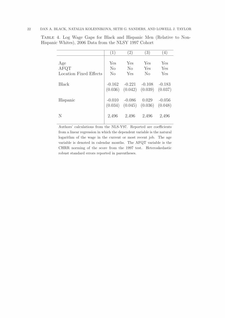
In Table 4, we repeat our empirical exercise using data from the 2006 survey for the 1997

NLSY cohort. Results are, if anything, even more dramatic. Comparing columns (3) and

(4) we see that inclusion of location fixed effects causes the estimated black-white gap to

decline from -0.11 to -0.18, i.e, by -0.07, and causes the estimated gap between Hispanics

and non-Hispanic whites to decline from 0.03 to -0.06, i.e., by -0.09.14

We view the results in Tables 3 and 4 as presenting compelling evidence of the importance

of conditioning location when comparing the earnings of groups with differing locations.

13As above, we study men only. We intend to look at racial wage differences for women in future work.14Interestingly, in comparison to the estimates for the 1979 cohort, there is a sharp decline in the magnitude

of the coefficient on the AFQT test. There are many possible explanation for this decline, we will mentionbut five. First, the cohorts are much different in age at this analysis: 25 to 32 for the 1979 and 22 to 26for the 1997. Participation patterns may differ dramatically between those ages, as well as by the type ofjobs held by respondents. Second, for the 1979 cohort, the Department of Defense provided the test scoresusing item response theory. For the 1997 cohort, however, the Department of Defense has been unwillingto provide the norming, so the test was normed by staff at the Center for Human Resources Research atOhio State without benefit of the individual test items. It is possible that the inability to use individual testitems may have substantially reduced the accuracy of the test norming. Third, the Department of Defencehas moved to computer assisted testing for the AFQT; it is possible that the new AFQT is less predictive ofcivilian labor market success. Fourth, it is, of course, possible that the economic rewards to cognitive skillsof young workers have declined, but this is, in our view, unlikely. Finally, the respondents in 1979 cohortwere much older – 15 to 23 – when they took the test than the 1997 cohort – 12 to 17. It is possible thatAFQT test is a less reliable predictor of labor market performance when given at young ages.


3. What if Preferences are Non-Homothetic?

The structural models we estimate above rely on homotheticity of individual preferences.

As it turns out, matters become substantially more complicated if preferences are not homo-

thetic. In particular, the steps we took in deriving equation (6) no longer pertain; equilibrium

racial wage disparity varies by location. We examine these issues by looking at two cases—

one in which there are location-specific differences in productivity and one in which there is

variation in local amenities.

Suppose also that minority workers have (unobserved) lower levels of human capital than

majority-group workers. Suppose also that there is variation across cities in productivity.15

The city with higher productivity will have higher wages and in consequence will typically

have higher housing prices. In this setting, we are interested in learning how race wage gaps

vary across locations.

Continue to let u1 and u0 be utility levels, respectively, of minority and majority workers.

Given that minority workers have a lower level of human capital, and thus within each city

lower wages, their utility will also be lower; u1 < u0. The disparity index in a given city

with a housing price p is I =e(p, u1)

e(p, u0).

We want to know how this index in a low-price, low-productivity city compares to the index

in a higher-price city. We conduct this thought experiment by evaluating the derivative of

the disparity index with respect to the housing price:

(14)∂I

∂p=

1

e(p, u0)2

[e(p, u0)

∂e(p, u1)

∂p− e(p, u1)

∂e(p, u0)

∂p

].

With a bit of algebraic manipulation we can rewrite (7):

(15)∂I

∂p=

e(p, u1)

pe(p, u0)

[p

e(p, u1)

∂e(p, u1)

∂p− p

e(p, u0)

∂e(p, u0)

∂p

].

Now Shephard’s lemma indicates that the derivative of the expenditure function with respect

to p is the demand for housing. So (15) can in turn can be written in terms of the budget

shares of housing for minority workers and majority workers, respectively s1H and s0

H :

(16)∂I

∂p=

e(p, u1)(s1H − s0

H)

pe(p, u0).

15While there has been much work on possible causes of such productivity differences (e.g., see Acemoglu,1996, Glaeser and Mare, 2001, and other work on agglomeration), we are agnostic here about the source ofthis variation.


This latter expression is positive if minority workers allocate a higher share of their income

to housing than do their majority counterparts. Given that minority workers have relatively

lower income, this amounts to the assumption that the income elasticity of housing is less

than one. As we mention above, there are some estimates that place the permanent income

elasticity of housing demand near one, but others do suggest that it is less than one.16 If so,

(17)∂I

∂p> 0.

Given that cities with relatively high productivity are also cities with higher housing prices

in this example, we expect that the wage disparity index will be higher in high-productivity

cities than in low-productivity cities. This means that for a disadvantaged minority, the

disparity index will be closer to 1; the proportional nominal wage gap will be smaller (in

absolute value) in the high-productivity city.

It is quite easy to explain the logic of this proposition. Suppose individuals live in one of

two locations—to take a concrete example, say Memphis and Chicago in 1940—and suppose

that in each location black workers (the minority in this example) earn less than their white

counterparts because of differences in human capital. Suppose further that all workers are

more productive in Chicago, owing perhaps to Chicago’s extensive railroad system and in-

dustrial agglomerates. In equilibrium we expect Chicago to have higher wages than Memphis

and also to have a relatively higher housing price. What about the black-white wage gap in

the two cities? Given that the elasticity of demand for housing is less than one, the relatively

high housing price in Chicago places a greater burden on the (poorer) black workers than the

(richer) white workers. Thus if both black and white workers are indifferent between living

in Memphis and Chicago, as they must be in equilibrium, black workers will require a larger

“Chicago wage premium” than will white workers; the proportional gap between black and

white wages will be smaller (in absolute value) in Chicago than in Memphis. This latter

outcome, of course, is what our derivation (17) shows.

Importantly, the same conclusion follows if the minority wage gap is instead generated

by labor market discrimination rather than human capital differences. Notice, first of all,

that under our assumption of costless mobility, a discriminated-against black worker will

be willing to live in either city, Memphis and Chicago, only if utility is the same in the

two locations. Thus the equilibrium condition (2) continues to hold, as do our subsequent

derivations, leading to (17). Again, the resulting wage disparity must be smaller in Chicago

16See, for example, Rosen (1985).


than in Memphis. Intuitively, the utility cost must be the same in the two places, and this

can happen only if the proportional wage gap is smaller in the location with higher housing

prices.

Another mechanism for generating price differentials across locations is differentials in

location-specific amenities. In general, the value of a location-specific amenity will vary

according to individuals’ incomes. For example, good public transportation might be more

valuable to individuals who cannot afford a car and good public education is more important

to people who don’t view private education as a viable option. Similarly, variety in gourmet

restaurants is typically more valuable to wealthy individuals. In turn, the value of amenities

will be correlated by race if there are race-related differences in income.

As in the example above (with location-specific differences in productivity), the equilib-

rium black-white wage gap varies across locations. But in this case we can be less certain

about the relationship between the black-white wage gap and housing prices.

Our theoretical analysis implies, in short, that there will likely be differences across cities

in equilibrium black-white wage gaps if our assumption of homothecitiy in preferences is

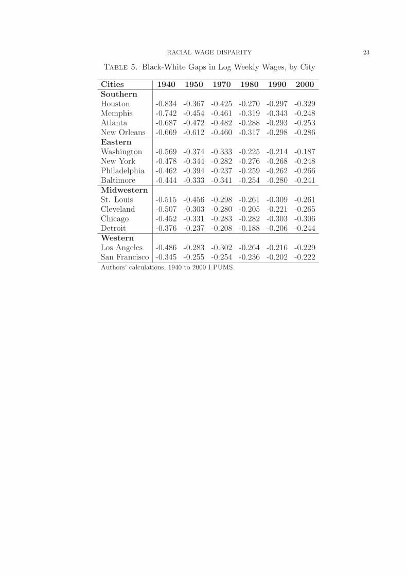
violated. With this in mind, we provide in Table 5 estimated black-white log wage gaps

for individual labor markets—for the 14 metropolitan areas with the largest black popula-

tion concentrations of black men in 1940. These estimates match on individuals’ age and

education (as in column (4) of Table 1).

The most striking feature of these statistics is the wide variation across cities in estimated

log wage gaps. Consider, for example, the estimates from 1940. Southern cities generally had

the largest gaps, and these gaps were in some cases are twice as large (in absolute values) as

the smallest observed gaps (in Detroit and San Francisco). If this variation is an equilibrium

phenomenon, it could reflect that productivity in general is higher in cities outside the South.

Of course there are other plausible explanations for this variation. For example, Charles

and Guryan (2008) emphasize that there is substantial variation across U.S. locations in

prejudice, and that this variation is responsible for some of the variation in black-white gaps

in wages. Also, Card and Krueger (1992) document that in the early part of the twentieth

century the quality of education afforded African American children was particularly poor

in much of the South. Both of these factors are surely at work in shaping the observed

patterns.


More generally, there is good reason to think that observed outcomes in 1940 are not an

equilibrium outcome. After all, this year was near the beginning of the epochal “second great

migration,” during which millions of African Americans migrated out of the South, in part,

no doubt, to escape poor economic conditions in the South. While we are convinced about

the value of thinking about racial wage gaps in an economically interpretable equilibrium

setting, we are mindful also that the equilibrium assumption is often unrealistic in location

models, and this concern might be especially germane for the application at hand.

Our general point, in any event, is that if we want to look at black-white wage convergence

in the U.S. since 1940 we miss a great deal if we simply look at national averages. Returning

to Table 4, which considers cities separately, we notice interesting differences in trends in

the black-white wage gap. In many cities, including New York and Philadelphia and all of

the Midwestern cities, there was virtually no narrowing of the black-white wage gap after

1970. Indeed, in Cleveland, Chicago, and Detroit, there was little change in the black-white

gap over the entire five decade span, 1950–2000. Observed declines in national black-white

gaps in large measure reflect the relocation of African Americans to these cities, rather than

black-white convergence that occurred uniformly across all locations.

4. Concluding Remarks

We have described a simple model in which prices vary across location. Our model ratio-

nalizes a very simple approach to estimating racial wage gaps. We show, in particular, that

the traditional approach of including a race indicator variable in a Mincer wage regression

provides an economically interpretable estimate if one includes location fixed effects in the

regression. Of course, many empirical analyses of the black-white wage gap do not include

such fixed effects. Thus we re-visit two important applications: (a) estimation of black-

white wage convergence, 1940-2000, and (b) estimation of the racial and ethnic wage gaps

that control for cognitive ability. In both cases we show that inference changes substantially

when we include fixed effects.

More generally, though, we present concerns about the assumptions that lead to our

structural model. In particular, if preferences are not homothetic, it is no longer the case

that the racial log wage gap is a constant across locations, even when the racial utility gap

is the same across locations (as it must be in equilibrium). Moreover, for many applications,

the equilibrium assumption is probably not tenable. A great deal of work remains to resolve


these issues as economists seek to better understand the nature of racial inequality in labor

markets.


Table 1. Black-White Gaps in Log Weekly Wage

(1) (2) (3) (4)Age Yes Yes Yes YesEducation No Yes No YesLocation No No Yes Yes1940 -0.741 -0.584 -0.662 -0.495

(0.0119) (0.0093) (0.0081) (0.0086)1950 -0.511 -0.400 -0.485 -0.365

(0.0139) (0.0110) (0.0108) (0.0125)1960 -0.510 -0.372 -0.489 -0.366

(0.0070) (0.0041) (0.0063) (0.0050)1970 -0.447 -0.315 -0.448 -0.329

(0.0138) (0.0057) (0.0054) (0.0047)1980 -0.308 -0.238 -0.332 -0.256

(0.0125) (0.0049) (0.0031) (0.0022)1990 -0.281 -0.212 -0.323 -0.248

(0.0054) (0.0054) (0.0027) (0.0022)2000 -0.301 -0.214 -0.358 -0.257

(0.0093) (0.0050) (0.0033) (0.0024)Source: Authors’ calculations, 1940 to 2000 I-PUMS. De-pendent variable is the logarithm of weekly earnings. Seethe data appendix for details.


Table 2. Location Indices for Black Men

(1) (2)Year Southern Residency Urban Residency1940 2.87 0.761950 2.48 0.911960 2.19 —1970 1.74 1.131980 1.69 1.181990 1.60 1.172000 1.59 1.15Notes: Authors’ calculations, 1940 to 2000 PUMS. Thesouthern residency index is the ratio of fraction black menaged 25 to 55 inclusive to white men of the same age. TheMSA residency index is, for similar aged men, the ratio ofblack men to white men residing in an MSA. The 1970 south-ern residency index is created using the 1 percent state sam-ple rather than the metro sample used in the rest of thispaper because region of residency is not uniquely identifiedfor MSAs that straddle the border of the southern region.


Table 3. Log Wage Gaps for Black and Hispanic Men (Relative to Non-Hispanic Whites), 1990 Data from the NLSY 1979 Cohort

(1) (2) (3) (4)

Age Yes Yes Yes YesAFQT No No Yes YesLocation Fixed Effects No Yes No Yes

Black -0.246 -0.283 -0.062 -0.128(0.021) (0.024) (0.022) (0.023)

Hispanic -0.110 -0.163 0.017 -0.039(0.025) (0.029) (0.025) (0.028)

N 4,206 4,206 4,206 4,206

Authors’ calculations from the NLS-Y79. Reported are coefficientsfrom a linear regression in which the dependent variable is the nat-ural logarithm of the wage in the current or most recent job. Theage variable is denoted in calendar months. The AFQT variable isthe 1989 renormed score from the 1981 test. Heteroskedastic robuststandard errors reported in parentheses.


Table 4. Log Wage Gaps for Black and Hispanic Men (Relative to Non-Hispanic Whites), 2006 Data from the NLSY 1997 Cohort

(1) (2) (3) (4)

Age Yes Yes Yes YesAFQT No No Yes YesLocation Fixed Effects No Yes No Yes

Black -0.162 -0.221 -0.108 -0.183(0.036) (0.042) (0.039) (0.037)

Hispanic -0.010 -0.086 0.029 -0.056(0.034) (0.045) (0.036) (0.048)

N 2,496 2,496 2,496 2,496

Authors’ calculations from the NLS-Y97. Reported are coefficientsfrom a linear regression in which the dependent variable is the naturallogarithm of the wage in the current or most recent job. The agevariable is denoted in calendar months. The AFQT variable is theCHRR norming of the score from the 1997 test. Heteroskedasticrobust standard errors reported in parentheses.


Table 5. Black-White Gaps in Log Weekly Wages, by City

Cities 1940 1950 1970 1980 1990 2000SouthernHouston -0.834 -0.367 -0.425 -0.270 -0.297 -0.329Memphis -0.742 -0.454 -0.461 -0.319 -0.343 -0.248Atlanta -0.687 -0.472 -0.482 -0.288 -0.293 -0.253New Orleans -0.669 -0.612 -0.460 -0.317 -0.298 -0.286EasternWashington -0.569 -0.374 -0.333 -0.225 -0.214 -0.187New York -0.478 -0.344 -0.282 -0.276 -0.268 -0.248Philadelphia -0.462 -0.394 -0.237 -0.259 -0.262 -0.266Baltimore -0.444 -0.333 -0.341 -0.254 -0.280 -0.241MidwesternSt. Louis -0.515 -0.456 -0.298 -0.261 -0.309 -0.261Cleveland -0.507 -0.303 -0.280 -0.205 -0.221 -0.265Chicago -0.452 -0.331 -0.283 -0.282 -0.303 -0.306Detroit -0.376 -0.237 -0.208 -0.188 -0.206 -0.244WesternLos Angeles -0.486 -0.283 -0.302 -0.264 -0.216 -0.229San Francisco -0.345 -0.255 -0.254 -0.236 -0.202 -0.222Authors’ calculations, 1940 to 2000 I-PUMS.


References

Acemoglu, Daron, 1996. “A Microfoundation for Social Increasing Returns in Human CapitalAccumulation,” Quarterly Journal of Economics, 111(3), 779-804.

Autor, D. and M. Duggan, 2003. “The Rise in the Disability Rolls and the Decline inUnemployment,” Quarterly Journal of Economics, 118 (1), 157-205.

Barron, John, Mark Berger, and Dan Black, 1997. “How Well Do We Measure Training?”Journal of Labor Economics July, 15(3), 507-528.

Baum-Snow, N. and D. Neal, 2009. “Mismeasurement of Usual Hours Worked in the Censusand ACS,” Economics Letters, 102 (1), 39-41.

Black, Dan A., 1995. “Discrimination in an Equilibrium Search Model,” Journal of LaborEconomics,13(2), 309-34.

Black, D., K. Daniel, and S. Sanders, 2002. “The Impact of Economic Conditions on Partic-ipation in Disability Programs: Evidence from the Coal Boom and Bust,” AmericanEconomic Review, 92 (1), 27-50.

Black, D., A. Haviland, S. Sanders, and L. Taylor, 2006. “Why Do Minority Men Earn Less?A Study of Wage Differentials among the Highly Educated,” The Review of Economicsand Statistics, 88 (2), 300-313.

Black, D., A. Haviland, S. Sanders, and L. Taylor, 2008. “Gender Wage Disparities Amongthe Highly Educated,” Journal of Human Resources, 43 (3), 630-659.

Black, Dan, Natalia Kolesnikova, and Lowell Taylor, 2009. “Earnings Functions When Wagesand Prices Vary by Location,” Journal of Labor Economics, 27(1), 21-47.

Black, Dan, Seth Sanders, and Lowell Taylor, 2003. “Measurement of Higher Education inthe Census and CPS,” Journal of the American Statistical Association, 98.

Bollinger, Christopher R., 2003. “Measurement Error in Human Capital and the Black-White Wage Gap,” Review of Economics and Statistics, 85(3), 578-85.

Card, David and Alan Kruger, 1992. “School Quality and Black-White Relative Earnings:A Direct Assessment,” Quarterly Journal of Economics 107, 151-200.

Chandra, Amitabh, 2000. Labor Market Dropouts and the Racial Wage Gap, 1940-1990.Unpublished dissertation, University of Kentucky.

Charles, Kerwin and Jonathan Guryan, 2008. “Prejudice and Wages: An Empirical Assess-ment of Becker’s The Economics of Discrimination,” Journal of Political Economy,116(5), 773-809.

DiNardo, J., N. Fortin, and T. Lemieux, 1996. “Labor Market Institutions and the Dis-tribution of Wages, 1973-1992: A Semiparametric Approach,” Econometrica, 64 (5),1001-1044.

Epple, Dennis, and Holger Sieg, 1999. 11Estimating Equilibrium Models of Local Jurisdic-tions,” Journal of Political Economy, 107(4), 645-681.

Glaeser, Edward L. and David C. Mare, 2001. “Cities and Skills,” Journal of Labor Eco-nomics, 19(2), 316-342.

Harmon, Oskar, 1988. “The Income Elasticities of Demand for Single-Family Owner-OccupiedHousing: An Empirical Reconciliation,” Journal of Urban Economics, 24, 173-185.

Haurin, Donald R., 1980. “The Regional Distribution of Population, Migration, and Cli-mate,” Quarterly Journal of Economics, 95(2), 293-808.

Haurin, Donald R., and Kyubang Lee, 1989. “A Structural Model of the Demand for Owner-Occupied Housing,” Journal of Urban Economics, 26 (3), 348-360.


Hirano, K., G. Imbens, and G. Ridder, 2003. “Efficient Estimation of Average TreatmentEffects Using the Estimated Propensity Score,” Econometrica, 71 (4), 1161-1189.

Mincer, Jacob, 1974. Schooling, Experience, and Earning. New York: National Bureau ofEconomic Research.

Neal, D., 2006. “Why has Black-White Skill Convergence Stopped?” in E. Hanushek andF. Welch (Eds.), Handbook of the Economics of Education, Volume 1, Chapter 9. Am-sterdam: Elsevier Science.

Neal, Derek A. and William R. Johnson, 1996. “The Role of Premarket Factors in Black-White Differences,” Journal of Political Economy, 104(5), 869-95.

O’Neill, June, 1990. “The Role of Human Capital in Earnings Differences Between Blackand White Men,” Journal of Economic Perspectives, 4(4), 25-45.

Roback, Jennifer, 1982. “Wages, Rents, and the Quality of Life,” The Journal of PoliticalEconomy, 90(6), 1257-1278.

Rosen, Harvey S., 1985. “Housing Subsidies: Effects on Housing Decisions, Efficiency, andEquity,” in Handbook of Public Economics, North-Holland, 375-420.

Ruggles, Steven, M. Sobek, T. Alexander, C. Fitch, R. Goeken, P. Kelly, M. King, andC. Ronnander, 2008. Integrated public use microdata series: Version 4.0. Technicalreport.

Samuleson, P. A. and S. Swamy, 1974. “Economic Index Numbers and Cannonical Duality:Survey and Syntheis,” American Economic Review, 64(4), 519-564.

Smith, James P. and Finis Welch, 1989. “Black Economic Progress After Myrdal,” Journalof Economic Literature, 27(2), 519-564.

Western, Bruce, 2006. Punishment and Inequality in America. New York: Russell SageFoundation.

Wooldridge, J., 2007. “Inverse Probability Weighted Estimation for General Missing DataProblems,” Journal of Econometrics, 141 (2), 1281-1301.


Data Appendix for Census Analysis

All the Census data for this paper are taken from IPUMS for the 1940 through 2000

Censuses; see Ruggles, Sobek, Alexander, Fitch, Goeken, Hall, King, and Ronnander (2008)

for details. The IPUMS represents an integrated data set of the Public Use Micro Samples

(PUMS) that were released in each of these Censuses.

Respondents were asked about their earnings in the previous year, the number of weeks

worked that year, and, at least for the 1980 to 2000 Censuses, the usual hours worked that

year. Baum-Snow and Neal (2009), however, document systematic biases that differ by race

and sex in responses to hours worked. We thus report results for both weekly earnings and

hourly earnings.

Our goal is to provide an analysis similar to that of Smith and Welch (1989). Toward that

end, we make many data-use decisions that parallel theirs, though there are differences that

we outline here. Like Smith and Welch we restrict our analysis to workers who work at least

27 weeks. As for age restrictions, Smith and Welch consider men aged 16 to 60. We are

concerned about the growth of enrollment in high school and college, and we do not want to

worry about decisions of “early retirement,” so we limit our analysis to men 25 to 55 inclusive.

To deal with the issue of schooling, Smith and Welch drop men from their sample who are

enrolled in school if they work less than 50 weeks a year. Given our age restrictions, we

find that adjustment to be unnecessary. Smith and Welch exclude unpaid family workers,

military personnel, and the self-employed who are not in agricultural. We also exclude

unpaid family workers, military personnel, the self-employed, and all agricultural workers.

Because of the increased mechanization of agricultural production in the U.S., there has

been a dramatic reduction in farm labor and a corresponding increase in the size of farms;

farming has become quite capital intensive. It is therefore difficult to separate the returns to

capital from the returns to labor. We exclude wage-and-salary agricultural workers because

payments to workers often involve payments in-kind, which makes the valuation of the wage

paid difficult. Of course, the exclusion of agricultural workers has little effect in 2000, but

represents a major exclusion for the early years. Excluding self-employed agricultural workers

has the added advantage of rendering the 1940 Census compatible with subsequent Decennial

Censuses, as the Census did not ask for farm earnings in 1940.


We also follow Smith and Welch in limiting the sample to workers whose reported weekly

earnings meet a minimum limit on weekly wages and an upper limit. The adopted limits are

as follows:

Lower limit of weekly earnings Upper limit of weekly earnings1940 1.50 1251950 3.25 2501960 6.25 6251970 10.00 1,2501980 19.80 1,8751990 35.00 3,0002000 45.00 4,000

The limits for 1940 to 1980 are taken from Smith and Welch (p. 522, footnote 5). For 1990

and 2000, we indexed the 1980 values to the CPI and rounded up.

An important concern with the Census data is item nonresponse. Respondents occasionally

choose not to answer questions about their age, race, ethnicity, or education level. More

frequently, respondents omit answers to questions about hours worked or earnings. Our

approach is to drop respondents who do not answer questions about age, race, Hispanic

status, education, or earnings. We do, however, increase the weights on other respondents

with identical ages, race, and education levels to reflect the missing data by using inverse

probability weighting. To be precise, we estimate the probably of a nonresponse, or

Pr(NR = 1|X = x0) = F (X0),

where x indexes the age-race-education-location cell, and then we construct weights,w1 ,

w1(x0) ≡ w0

1− F (x0),

where w0 are the initial Census weights. Thus, if half the people in the age-race-education-

location cell do not respond to their earnings or hours worked questions, the responders

within the cell have their weights doubled (see Wooldridge (2007)). This procedure implic-

itly assumes that data are, conditional on the age-race-education-location cell, missing at

random. Because we condition on age, race, education, and location, this procedure also

replicates the Census joint distribution of the age-race-education-location variables.

We also face two additional important issues about the data: the measurement of education

and the measurement of location. The measurement of education in the Censuses presents

problems for at least three reasons. First, in 1990, the Census Bureau reworked the education


question to account for highest degree for those with a college education and some categorical

data for lower levels of education. For instance, in 1990 the Census asked: How much school

has this person COMPLETED? Fill ONE circle for the highest level COMPLETED or degree

RECEIVED. If currently enrolled, mark the level of previous grade attended or highest degree

received. Response options were:

◦ No school completed ◦ Nursery school◦ Kindergarten◦ 1st, 2nd, 3rd, or 4th grade◦ 5th, 6th, 7th, or 8th grade◦ 9th grade◦ 10th grade◦ 11th grade◦ 12th grade, NO DIPLOMA◦ HIGH SCHOOL GRADUATE - high school DIPLOMA or the equivalent (e.g., GED)◦ Some college but no degree◦ Associate degree in college - Occupational program◦ Associate degree in college - Academic program◦ Bachelor’s degree (For example: BA, AB, BS)◦ Master’s degree (For example: MA, MS, MEng, MEd, MSW, MBA)◦ Professional school degree (For example: MD, DDS, DVM, LLB, JD)◦ Doctorate degree (For example: PhD, EdD)

Prior to 1990, the Census asked instead about “years of schooling.” For instance, in 1980

the Census asked: What is the highest grade (or year) of regular school this person has ever

attended? Fill one circle. If now attending school, mark grade person is in. If high school

was finished by equivalency test (GED), mark “12”. Response options for highest grade

attended were ◦ Never attended school, ◦ Nursery school, ◦ Kindergarten, and these further

options:

Elementary through high school (grade or year)1 2 3 4 5 6 7 8 9 10 11 12◦ ◦ ◦ ◦ ◦ ◦ ◦ ◦ ◦ ◦ ◦ ◦

College (academic years)1 2 3 4 5 6 7 8 or more◦ ◦ ◦ ◦ ◦ ◦ ◦ ◦

Drawing consistent inferences with schooling data drawn these two ways is in principle

quite simple if the two types of questions have a similar structure of measurement error.

Unfortunately, for the 1990 Census, Black, Sanders, and Taylor (2003) document that the


education questions exhibit significant measurement error and that the degree of measure-

ment error is correlated with race. Moreover, there was a dramatic increase in the educational

attainment of Americans over the period. For instance, in 1940 88 percent of blacks and 64

percent of whites between the ages of 25 and 60 did not have a high school education, and

only 2 percent of blacks and 8 percent of whites had a bachelor’s degree or better. By 2000,

only 9 percent of blacks and 5 percent of whites did not have a high school degree while fully

33 percent of whites and over 19 percent of blacks had a bachelor’s degree or better.

In our regression analysis we treat education in a non-parametric way, and given the avail-

able data, we use the following ten education categories: no formal education or kindergarten

only, 1 to 4 years, 5 to 8 years, 9 years, 10 years, 11 years, 12 years, some college but no

bachelor’s degree, bachelor’s degree, and more than a bachelor’s degree.

Finally, there is the issue of the measurement of location. Because of the growth in cities

and changes in disclosure policy, the identification of metropolitan statistical areas (MSAs)

varies over time. In 1960 (the first public use micro sample that the Census Bureau released),

the only geography identified was State of residence. As a result, we cannot conduct the

same location analysis of interest to us with the 1960 data; we use only an urban indicator

interacted with an indicator for state of residence. In 1940, 1950, and 1970 through 2000,

we use MSA of residence for those respondents living in a MSA. For those respondents not

living in an identified MSA, we use an indicator for state of residence. Hence, we exploit the

geographical variation that is generally available to us. There are, however, a few additional

noteworthy limitations:

First, residents of some current MSA’s are not separately identified in the early censuses,

but are so identified subsequently. For example, in the 1940, Orlando residents are treated as

individuals living in “rural” Florida, but in later years are broken out as part of an Orlando

MSA. Similarly, Las Vegas is identified only starting in 1970. There are a host of smaller

towns that are only identified in later years. Moreover, MSAs can be created from regions

that were previously a part of different MSAs. This is a particular problem in the densely

populated areas of the east and west coasts. Finally, for areas that are only identified as

“rural” we may be mixing residents from very different areas of a given state. For example,

this designation mixes residents of the desert areas of Southern California with residents of

rural Northern California, who may face very different labor markets and price levels.


For the 1940 through 1970 Censuses, we use a one-percent sample of respondents, and from

1980 to 2000, we use the five-percent sample, which, along with population growth, provides

much larger sample sizes and much more precise estimates. Prior to 1980, the Census did

not release the five-percent sample so we do not have access the extremely large sample sizes

that the five-percent sample affords. Finally, we note one important data limitation with

the 1950 Census. In 1950, only the “sample line” respondents were asked about education

and earnings by the Census Bureau. Hence, only about 3.3 percent of the population was

given these questions. Thus, estimates from the 1950 Census are considerably less precise

than estimates from even the 1940 Census.

In 1960 and 1970, the Census asked only for hours of work and weeks of work on intervals.

To impute the actual levels, we took information from the 1980 Census and calculated the

average weeks (or average hours) conditional on the being in the relevant category. In the

table on the next page we provide the values that we used for the imputations.

Interval Imputed weeks Interval Imputed hours1-13 weeks 1.1 1-14 hours 8.5714-26 weeks 21.4 15-29 hours 21.9527-39 weeks 33.3 30-34 hours 30.6440-47 weeks 43.4 35-39 hours 36.3548-49 weeks 48.3 40 hours 4050-52 weeks 51.8 41-48 hours 45.46

49-59 hours 51.4160 or more hours 67.02

Prior to 1980, the Census did not ask the usual hours worked so we used hours last week

as a proxy. In 1980, conditional on both reports being positive, the correlation is only 0.61.

While quite low, this correlation is not materially different than those found in validation

studies; see Barron, Berger, and Black (1997) for a discussion.

the role of location in evaluating racial wage...

Documents