HAL Id: hal-01778028https://hal.univ-reunion.fr/hal-01778028

Preprint submitted on 25 Apr 2018

HAL is a multi-disciplinary open accessarchive for the deposit and dissemination of sci-entific research documents, whether they are pub-lished or not. The documents may come fromteaching and research institutions in France orabroad, or from public or private research centers.

L’archive ouverte pluridisciplinaire HAL, estdestinée au dépôt et à la diffusion de documentsscientifiques de niveau recherche, publiés ou non,émanant des établissements d’enseignement et derecherche français ou étrangers, des laboratoirespublics ou privés.

The Significant Impact of Abstentions on ElectionOutcomes

William V. Gehrlein, Dominique Lepelley

To cite this version:William V. Gehrlein, Dominique Lepelley. The Significant Impact of Abstentions on Election Out-comes. 2018. �hal-01778028�

1

The Significant Impact of Abstentions on Election Outcomes

23 April 2018

William V. Gehrlein

Department of Business Administration, University of Delaware

Newark, DE 19716, USA

wvg@udel.edu

Dominique Lepelley

Department of Economics, University of La Réunion

Saint-Denis cedex, La Réunion, France

dominique.lepelley@univ-reunion.fr

Abstract

Two approaches are considered in an attempt to mollify previous observations regarding the very

negative impact that voter abstentions can have on Plurality Rule, Negative Plurality Rule and

Borda Rule when voters’ preferences are assumed to be statistically independent. The first

option is to add a degree of dependence among voters’ preferences, and the second is to consider

extensions of these three voting rules by using each as the basis for a two-stage elimination

election procedure. The end result in both cases is that improved results are indeed observed for

both Condorcet Efficiency and the probability that a Borda Paradox is observed for larger values

of voter participation rates. The very disturbing result is that both of these options actually tend

to make things worse with voter participation rates of 40% or less, and voter participation rates

are observed in practice at this level.

Introduction

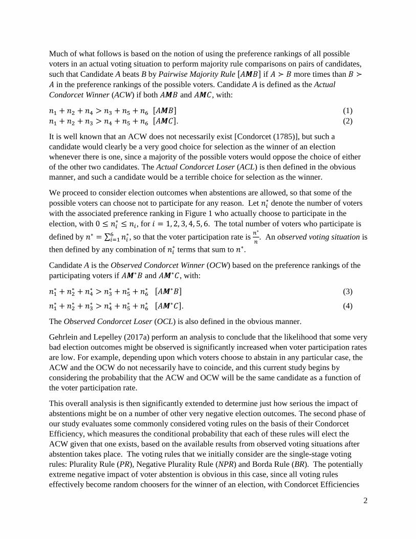
We consider the impact that voter abstention can have on elections with three candidates

{𝐴, 𝐵, 𝐶} when there are n possible voters in the electorate. To begin, we define the preferences

of these voters by using 𝐴 ≻ 𝐵 to denote the fact that any given voter prefers Candidate A to

Candidate B. There are six possible linear voter preference rankings on these candidates that are

transitive and have no voter indifference between candidates, as shown in Figure 1.

A A B C B C

B C A A C B

C B C B A A

𝑛1 𝑛2 𝑛3 𝑛4 𝑛5 𝑛6

Figure 1. Six possible linear preference rankings on three candidates.

Here, for example, 𝑛1 represents the number of possible voters with the preference ranking 𝐴 ≻

𝐵 ≻ 𝐶, with 𝐴 ≻ 𝐶 being required by transitivity. The total number of possible voters is n with

𝑛 = ∑ 𝑛𝑖6𝑖=1 , and an actual voting situation defines any combination of 𝑛𝑖 terms that sum to n.

2

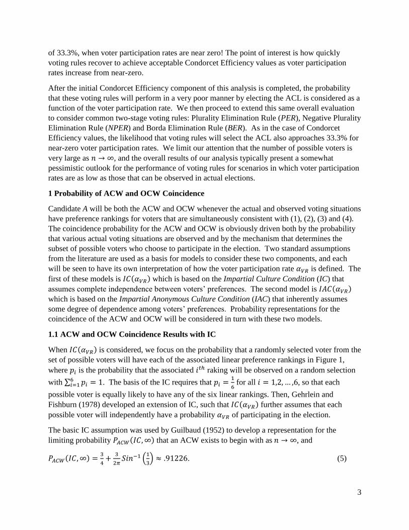
Much of what follows is based on the notion of using the preference rankings of all possible

voters in an actual voting situation to perform majority rule comparisons on pairs of candidates,

such that Candidate A beats B by Pairwise Majority Rule [𝐴𝑴𝐵] if 𝐴 ≻ 𝐵 more times than 𝐵 ≻

𝐴 in the preference rankings of the possible voters. Candidate A is defined as the Actual

Condorcet Winner (ACW) if both 𝐴𝑴𝐵 and 𝐴𝑴𝐶, with:

𝑛1 + 𝑛2 + 𝑛4 > 𝑛3 + 𝑛5 + 𝑛6 [𝐴𝑴𝐵] (1)

𝑛1 + 𝑛2 + 𝑛3 > 𝑛4 + 𝑛5 + 𝑛6 [𝐴𝑴𝐶]. (2)

It is well known that an ACW does not necessarily exist [Condorcet (1785)], but such a

candidate would clearly be a very good choice for selection as the winner of an election

whenever there is one, since a majority of the possible voters would oppose the choice of either

of the other two candidates. The Actual Condorcet Loser (ACL) is then defined in the obvious

manner, and such a candidate would be a terrible choice for selection as the winner.

We proceed to consider election outcomes when abstentions are allowed, so that some of the

possible voters can choose not to participate for any reason. Let 𝑛𝑖∗ denote the number of voters

with the associated preference ranking in Figure 1 who actually choose to participate in the

election, with 0 ≤ 𝑛𝑖∗ ≤ 𝑛𝑖, for 𝑖 = 1, 2, 3, 4, 5, 6. The total number of voters who participate is

defined by 𝑛∗ = ∑ 𝑛𝑖∗6

𝑖=1 , so that the voter participation rate is 𝑛∗

𝑛. An observed voting situation is

then defined by any combination of 𝑛𝑖∗ terms that sum to 𝑛∗.

Candidate A is the Observed Condorcet Winner (OCW) based on the preference rankings of the

participating voters if 𝐴𝑴∗𝐵 and 𝐴𝑴∗𝐶, with:

𝑛1∗ + 𝑛2

∗ + 𝑛4∗ > 𝑛3

∗ + 𝑛5∗ + 𝑛6

∗ [𝐴𝑴∗𝐵] (3)

𝑛1∗ + 𝑛2

∗ + 𝑛3∗ > 𝑛4

∗ + 𝑛5∗ + 𝑛6

∗ [𝐴𝑴∗𝐶]. (4)

The Observed Condorcet Loser (OCL) is also defined in the obvious manner.

Gehrlein and Lepelley (2017a) perform an analysis to conclude that the likelihood that some very

bad election outcomes might be observed is significantly increased when voter participation rates

are low. For example, depending upon which voters choose to abstain in any particular case, the

ACW and the OCW do not necessarily have to coincide, and this current study begins by

considering the probability that the ACW and OCW will be the same candidate as a function of

the voter participation rate.

This overall analysis is then significantly extended to determine just how serious the impact of

abstentions might be on a number of other very negative election outcomes. The second phase of

our study evaluates some commonly considered voting rules on the basis of their Condorcet

Efficiency, which measures the conditional probability that each of these rules will elect the

ACW given that one exists, based on the available results from observed voting situations after

abstention takes place. The voting rules that we initially consider are the single-stage voting

rules: Plurality Rule (PR), Negative Plurality Rule (NPR) and Borda Rule (BR). The potentially

extreme negative impact of voter abstention is obvious in this case, since all voting rules

effectively become random choosers for the winner of an election, with Condorcet Efficiencies

3

of 33.3%, when voter participation rates are near zero! The point of interest is how quickly

voting rules recover to achieve acceptable Condorcet Efficiency values as voter participation

rates increase from near-zero.

After the initial Condorcet Efficiency component of this analysis is completed, the probability

that these voting rules will perform in a very poor manner by electing the ACL is considered as a

function of the voter participation rate. We then proceed to extend this same overall evaluation

to consider common two-stage voting rules: Plurality Elimination Rule (PER), Negative Plurality

Elimination Rule (NPER) and Borda Elimination Rule (BER). As in the case of Condorcet

Efficiency values, the likelihood that voting rules will select the ACL also approaches 33.3% for

near-zero voter participation rates. We limit our attention that the number of possible voters is

very large as 𝑛 → ∞, and the overall results of our analysis typically present a somewhat

pessimistic outlook for the performance of voting rules for scenarios in which voter participation

rates are as low as those that can be observed in actual elections.

1 Probability of ACW and OCW Coincidence

Candidate A will be both the ACW and OCW whenever the actual and observed voting situations

have preference rankings for voters that are simultaneously consistent with (1), (2), (3) and (4).

The coincidence probability for the ACW and OCW is obviously driven both by the probability

that various actual voting situations are observed and by the mechanism that determines the

subset of possible voters who choose to participate in the election. Two standard assumptions

from the literature are used as a basis for models to consider these two components, and each

will be seen to have its own interpretation of how the voter participation rate 𝛼𝑉𝑅 is defined. The

first of these models is 𝐼𝐶(𝛼𝑉𝑅) which is based on the Impartial Culture Condition (IC) that

assumes complete independence between voters’ preferences. The second model is 𝐼𝐴𝐶(𝛼𝑉𝑅)

which is based on the Impartial Anonymous Culture Condition (IAC) that inherently assumes

some degree of dependence among voters’ preferences. Probability representations for the

coincidence of the ACW and OCW will be considered in turn with these two models.

1.1 ACW and OCW Coincidence Results with IC

When 𝐼𝐶(𝛼𝑉𝑅) is considered, we focus on the probability that a randomly selected voter from the

set of possible voters will have each of the associated linear preference rankings in Figure 1,

where 𝑝𝑖 is the probability that the associated 𝑖𝑡ℎ raking will be observed on a random selection

with ∑ 𝑝𝑖6𝑖=1 = 1. The basis of the IC requires that 𝑝𝑖 =

1

6 for all 𝑖 = 1,2, … ,6, so that each

possible voter is equally likely to have any of the six linear rankings. Then, Gehrlein and

Fishburn (1978) developed an extension of IC, such that 𝐼𝐶(𝛼𝑉𝑅) further assumes that each

possible voter will independently have a probability 𝛼𝑉𝑅 of participating in the election.

The basic IC assumption was used by Guilbaud (1952) to develop a representation for the

limiting probability 𝑃𝐴𝐶𝑊(𝐼𝐶,∞) that an ACW exists to begin with as 𝑛 → ∞, and

𝑃𝐴𝐶𝑊(𝐼𝐶,∞) =3

4+

3

2𝜋𝑆𝑖𝑛−1 (

1

3) ≈ .91226. (5)

4

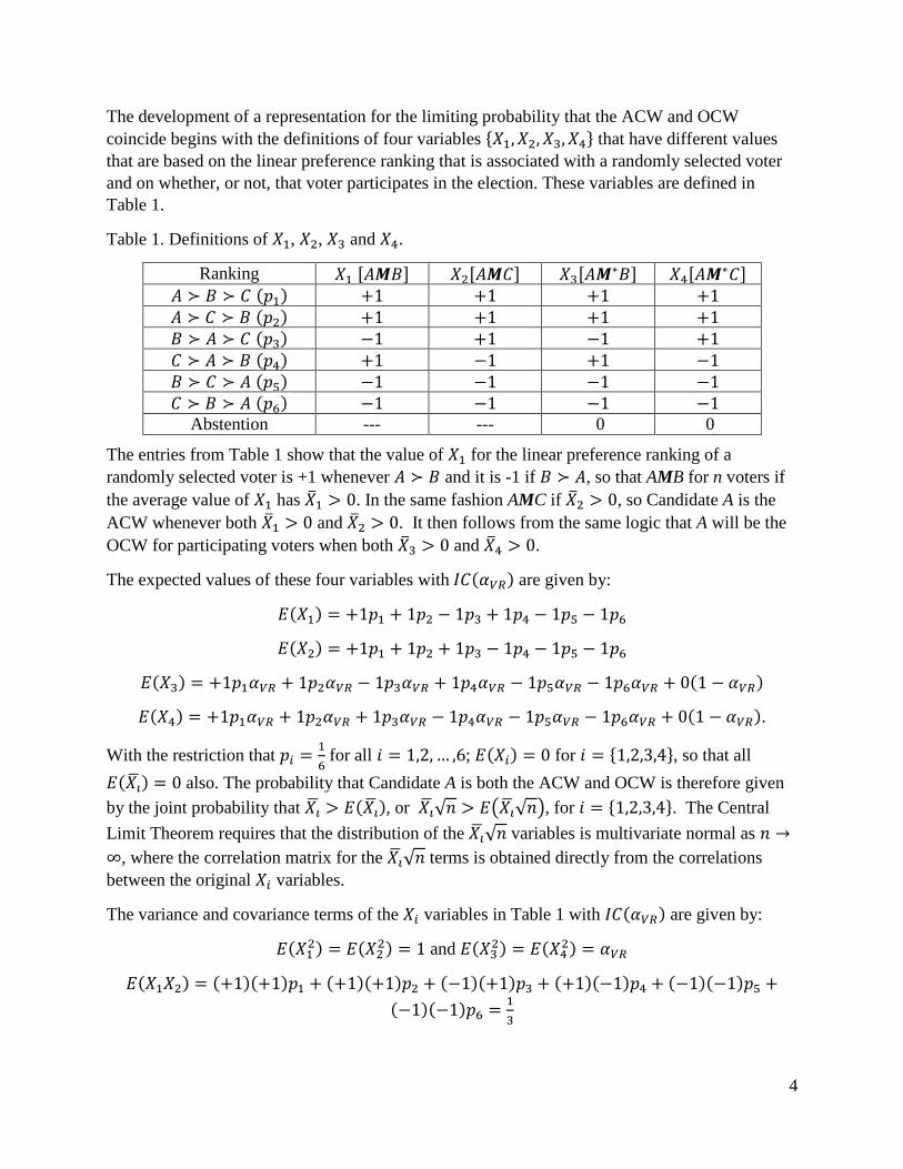
The development of a representation for the limiting probability that the ACW and OCW

coincide begins with the definitions of four variables {𝑋1, 𝑋2, 𝑋3, 𝑋4} that have different values

that are based on the linear preference ranking that is associated with a randomly selected voter

and on whether, or not, that voter participates in the election. These variables are defined in

Table 1.

Table 1. Definitions of 𝑋1, 𝑋2, 𝑋3 and 𝑋4.

Ranking 𝑋1 [𝐴𝑴𝐵] 𝑋2[𝐴𝑴𝐶] 𝑋3[𝐴𝑴∗𝐵] 𝑋4[𝐴𝑴∗𝐶] 𝐴 ≻ 𝐵 ≻ 𝐶 (𝑝1) +1 +1 +1 +1

𝐴 ≻ 𝐶 ≻ 𝐵 (𝑝2) +1 +1 +1 +1

𝐵 ≻ 𝐴 ≻ 𝐶 (𝑝3) −1 +1 −1 +1

𝐶 ≻ 𝐴 ≻ 𝐵 (𝑝4) +1 −1 +1 −1

𝐵 ≻ 𝐶 ≻ 𝐴 (𝑝5) −1 −1 −1 −1

𝐶 ≻ 𝐵 ≻ 𝐴 (𝑝6) −1 −1 −1 −1

Abstention --- --- 0 0

The entries from Table 1 show that the value of 𝑋1 for the linear preference ranking of a

randomly selected voter is +1 whenever 𝐴 ≻ 𝐵 and it is -1 if 𝐵 ≻ 𝐴, so that AMB for n voters if

the average value of 𝑋1 has �̅�1 > 0. In the same fashion AMC if �̅�2 > 0, so Candidate A is the

ACW whenever both �̅�1 > 0 and �̅�2 > 0. It then follows from the same logic that A will be the

OCW for participating voters when both �̅�3 > 0 and �̅�4 > 0.

The expected values of these four variables with 𝐼𝐶(𝛼𝑉𝑅) are given by:

𝐸(𝑋1) = +1𝑝1 + 1𝑝2 − 1𝑝3 + 1𝑝4 − 1𝑝5 − 1𝑝6

𝐸(𝑋2) = +1𝑝1 + 1𝑝2 + 1𝑝3 − 1𝑝4 − 1𝑝5 − 1𝑝6

𝐸(𝑋3) = +1𝑝1𝛼𝑉𝑅 + 1𝑝2𝛼𝑉𝑅 − 1𝑝3𝛼𝑉𝑅 + 1𝑝4𝛼𝑉𝑅 − 1𝑝5𝛼𝑉𝑅 − 1𝑝6𝛼𝑉𝑅 + 0(1 − 𝛼𝑉𝑅)

𝐸(𝑋4) = +1𝑝1𝛼𝑉𝑅 + 1𝑝2𝛼𝑉𝑅 + 1𝑝3𝛼𝑉𝑅 − 1𝑝4𝛼𝑉𝑅 − 1𝑝5𝛼𝑉𝑅 − 1𝑝6𝛼𝑉𝑅 + 0(1 − 𝛼𝑉𝑅).

With the restriction that 𝑝𝑖 =1

6 for all 𝑖 = 1,2, … ,6; 𝐸(𝑋𝑖) = 0 for 𝑖 = {1,2,3,4}, so that all

𝐸(𝑋�̅�) = 0 also. The probability that Candidate A is both the ACW and OCW is therefore given

by the joint probability that 𝑋�̅� > 𝐸(𝑋�̅�), or 𝑋�̅�√𝑛 > 𝐸(𝑋�̅�√𝑛), for 𝑖 = {1,2,3,4}. The Central

Limit Theorem requires that the distribution of the 𝑋�̅�√𝑛 variables is multivariate normal as 𝑛 →

∞, where the correlation matrix for the 𝑋�̅�√𝑛 terms is obtained directly from the correlations

between the original 𝑋𝑖 variables.

The variance and covariance terms of the 𝑋𝑖 variables in Table 1 with 𝐼𝐶(𝛼𝑉𝑅) are given by:

𝐸(𝑋12) = 𝐸(𝑋2

2) = 1 and 𝐸(𝑋32) = 𝐸(𝑋4

2) = 𝛼𝑉𝑅

𝐸(𝑋1𝑋2) = (+1)(+1)𝑝1 + (+1)(+1)𝑝2 + (−1)(+1)𝑝3 + (+1)(−1)𝑝4 + (−1)(−1)𝑝5 +

(−1)(−1)𝑝6 =1

3

5

𝐸(𝑋1𝑋3) = (+1)(+1)𝑝1𝛼𝑉𝑅 + (+1)(+1)𝑝2𝛼𝑉𝑅 + (−1)(−1)𝑝3𝛼𝑉𝑅 + (+1)(+1)𝑝4𝛼𝑉𝑅 +(−1)(−1)𝑝5𝛼𝑉𝑅 + (−1)(−1)𝑝6𝛼𝑉𝑅 + 0(1 − 𝛼𝑉𝑅) = 𝛼𝑉𝑅

𝐸(𝑋1𝑋4) = (+1)(+1)𝑝1𝛼𝑉𝑅 + (+1)(+1)𝑝2𝛼𝑉𝑅 + (−1)(+1)𝑝3𝛼𝑉𝑅 + (+1)(−1)𝑝4𝛼𝑉𝑅 +

(−1)(−1)𝑝5𝛼𝑉𝑅 + (−1)(−1)𝑝6𝛼𝑉𝑅 + 0(1 − 𝛼𝑉𝑅) =𝛼𝑉𝑅

3

𝐸(𝑋2𝑋3) = (+1)(+1)𝑝1𝛼𝑉𝑅 + (+1)(+1)𝑝2𝛼𝑉𝑅 + (+1)(−1)𝑝3𝛼𝑉𝑅 + (−1)(+1)𝑝4𝛼𝑉𝑅 +

(−1)(−1)𝑝5𝛼𝑉𝑅 + (−1)(−1)𝑝6𝛼𝑉𝑅 + 0(1 − 𝛼𝑉𝑅) =𝛼𝑉𝑅

3

𝐸(𝑋2𝑋4) = (+1)(+1)𝑝1𝛼𝑉𝑅 + (+1)(+1)𝑝2𝛼𝑉𝑅 + (+1)(+1)𝑝3𝛼𝑉𝑅 + (−1)(−1)𝑝4𝛼𝑉𝑅 +(−1)(−1)𝑝5𝛼𝑉𝑅 + (−1)(−1)𝑝6𝛼𝑉𝑅 + 0(1 − 𝛼𝑉𝑅) = 𝛼𝑉𝑅

𝐸(𝑋3𝑋4) = (+1)(+1)𝑝1𝛼𝑉𝑅 + (+1)(+1)𝑝2𝛼𝑉𝑅 + (−1)(+1)𝑝3𝛼𝑉𝑅 + (+1)(−1)𝑝4𝛼𝑉𝑅 +

(−1)(−1)𝑝5𝛼𝑉𝑅 + (−1)(−1)𝑝6𝛼𝑉𝑅 + 0(1 − 𝛼𝑉𝑅) =𝛼𝑉𝑅

3.

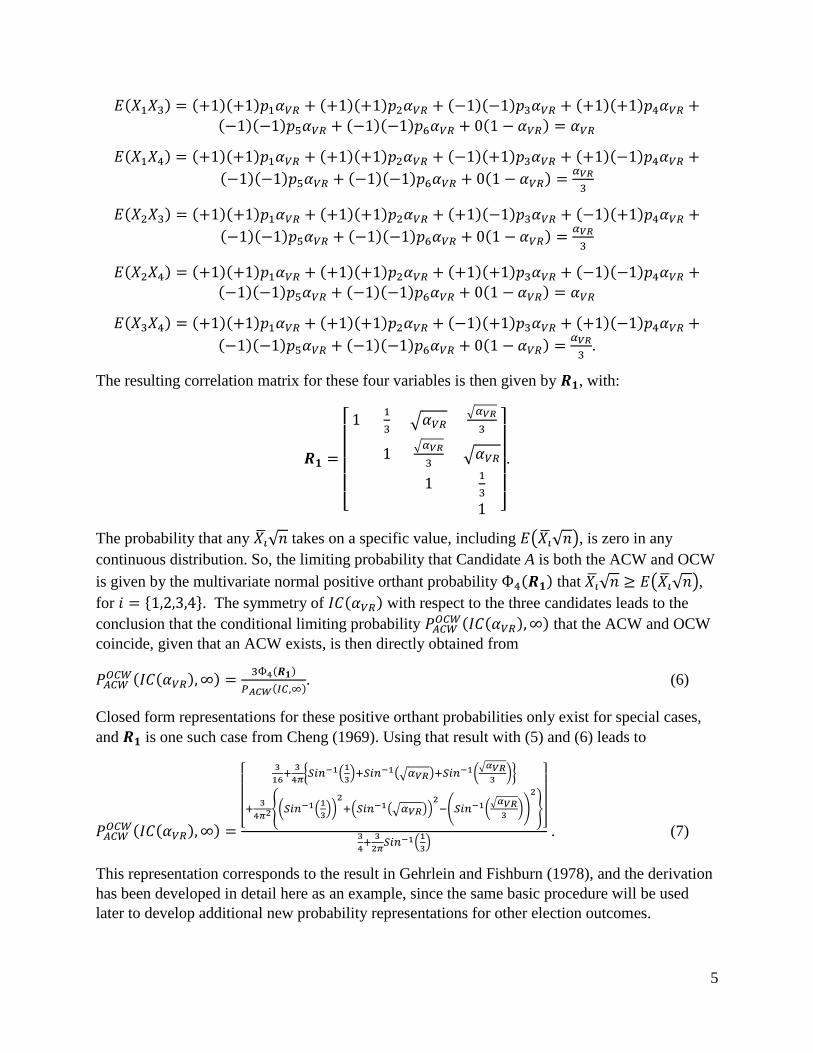
The resulting correlation matrix for these four variables is then given by 𝑹𝟏, with:

𝑹𝟏 =

[ 1

1

3√𝛼𝑉𝑅

√𝛼𝑉𝑅

3

1√𝛼𝑉𝑅

3√𝛼𝑉𝑅

11

3

1 ]

.

The probability that any 𝑋�̅�√𝑛 takes on a specific value, including 𝐸(𝑋�̅�√𝑛), is zero in any

continuous distribution. So, the limiting probability that Candidate A is both the ACW and OCW

is given by the multivariate normal positive orthant probability Ф4(𝑹𝟏) that 𝑋�̅�√𝑛 ≥ 𝐸(𝑋�̅�√𝑛),

for 𝑖 = {1,2,3,4}. The symmetry of 𝐼𝐶(𝛼𝑉𝑅) with respect to the three candidates leads to the

conclusion that the conditional limiting probability 𝑃𝐴𝐶𝑊𝑂𝐶𝑊(𝐼𝐶(𝛼𝑉𝑅),∞) that the ACW and OCW

coincide, given that an ACW exists, is then directly obtained from

𝑃𝐴𝐶𝑊𝑂𝐶𝑊(𝐼𝐶(𝛼𝑉𝑅),∞) =

3Ф4(𝑹𝟏)

𝑃𝐴𝐶𝑊(𝐼𝐶,∞). (6)

Closed form representations for these positive orthant probabilities only exist for special cases,

and 𝑹𝟏 is one such case from Cheng (1969). Using that result with (5) and (6) leads to

𝑃𝐴𝐶𝑊𝑂𝐶𝑊(𝐼𝐶(𝛼𝑉𝑅),∞) =

[

3

16+

3

4𝜋{𝑆𝑖𝑛−1(

1

3)+𝑆𝑖𝑛−1(√𝛼𝑉𝑅)+𝑆𝑖𝑛−1(

√𝛼𝑉𝑅3

)}

+3

4𝜋2{(𝑆𝑖𝑛−1(1

3))

2

+(𝑆𝑖𝑛−1(√𝛼𝑉𝑅))2−(𝑆𝑖𝑛−1(

√𝛼𝑉𝑅3

))

2

}

]

3

4+

3

2𝜋𝑆𝑖𝑛−1(

1

3)

. (7)

This representation corresponds to the result in Gehrlein and Fishburn (1978), and the derivation

has been developed in detail here as an example, since the same basic procedure will be used

later to develop additional new probability representations for other election outcomes.

6

There is no election output to evaluate without any voter participation when 𝛼𝑉𝑅 = 0, so Table 2

lists values of 𝑃𝐴𝐶𝑊𝑂𝐶𝑊(𝐼𝐶(𝛼𝑉𝑅),∞) from (7) for 𝛼𝑉𝑅 → 0 and for each 𝛼𝑉𝑅 = .1(. 1)1.0.

Table 2. Limiting ACW and OCW Coincidence Probabilities.

𝛼𝑉𝑅 𝐼𝐶(𝛼𝑉𝑅) 𝐼𝐴𝐶(𝛼𝑉𝑅) ≈ 0 .3041 5/16 = .3125

.1 .4236 .3482

.2 .4806 .3949

.3 .5290 .4564

.4 .5742 .5357

.5 .6186 .6310

.6 .6640 .7291

.7 .7126 .8160

.8 .7675 .8887

.9 .8365 .9492

1.0 1.0000 1.0000

Some results from the 𝑃𝐴𝐶𝑊𝑂𝐶𝑊 (𝐼𝐶(𝛼𝑉𝑅),∞) values in Table 2 are predictable. In particular, the

coincidence probability is one when all voters participate with 𝛼𝑉𝑅 = 1, and the coincidence

probability decreases as this participation rate declines. When almost all voters independently

abstain as 𝛼𝑉𝑅 → 0, the candidate that becomes the OCW is effectively selected at random if

there is an OCW, so the coincidence probability goes to 1

3𝑃𝐴𝐶𝑊(𝐼𝐶,∞). What is surprising is the

very steep rate of decline in 𝑃𝐴𝐶𝑊𝑂𝐶𝑊(𝐼𝐶(𝛼𝑉𝑅),∞) values as 𝛼𝑉𝑅 decreases, with only about a 62%

chance of coincidence when 𝛼𝑉𝑅 = .5. Low voter participation rates can clearly have a huge

negative impact on election outcomes with the independent voter 𝐼𝐶(𝛼𝑉𝑅) scenario.

1.2 ACW and OCW Coincidence Results with IAC

It is well known that the introduction of a degree of dependence among voters’ preferences

generally reduces the probability that most paradoxical election outcomes will be observed,

relative to the case of complete independence with IC [see for example Gehrlein and Lepelley

(2011)]. Gehrlein and Lepelley (2017b) investigated this impact on the conditional probability

for AOW and OCW coincidence with the assumption of 𝐼𝐴𝐶(𝛼𝑉𝑅), such that all actual and

observed voting situations are equally likely to be observed, given that the voter participation

rate is fixed at 𝛼𝑉𝑅 =𝑛∗

𝑛.

To begin developing this representation for the coincidence probability of ACW and OCW with

𝐼𝐴𝐶(𝛼𝑉𝑅), we note that this requires that (1), (2), (3) and (4) must hold, along with

𝑛1 + 𝑛2 + 𝑛3 + 𝑛4 + 𝑛5 + 𝑛6 = 𝑛 (8)

𝑛1∗ + 𝑛2

∗ + 𝑛3∗ + 𝑛4

∗ + 𝑛5∗ + 𝑛6

∗ = 𝑛∗ (9)

0 ≤ 𝑛𝑖∗ ≤ 𝑛𝑖, for 𝑖 = 1, 2, 3, 4, 5, 6 (10)

We would start by obtaining a representation for the total number of voting situations for which

the restrictions (1), (2), (3), (4), (8), (9) and (10) simultaneously apply as a function of n and 𝑛∗,

7

and then divide that by the total number of voting situations for which (1), (2), (8), (9) and (10)

simultaneously apply as a function of n and 𝑛∗. The final representation could then be expressed

as a function of n and 𝛼𝑉𝑅.

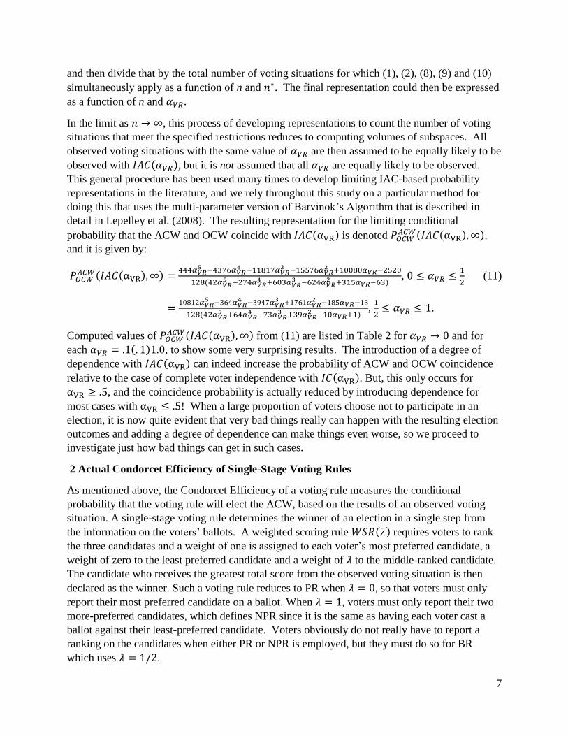
In the limit as 𝑛 → ∞, this process of developing representations to count the number of voting

situations that meet the specified restrictions reduces to computing volumes of subspaces. All

observed voting situations with the same value of 𝛼𝑉𝑅 are then assumed to be equally likely to be

observed with 𝐼𝐴𝐶(𝛼𝑉𝑅), but it is not assumed that all 𝛼𝑉𝑅 are equally likely to be observed.

This general procedure has been used many times to develop limiting IAC-based probability

representations in the literature, and we rely throughout this study on a particular method for

doing this that uses the multi-parameter version of Barvinok’s Algorithm that is described in

detail in Lepelley et al. (2008). The resulting representation for the limiting conditional

probability that the ACW and OCW coincide with 𝐼𝐴𝐶(αVR) is denoted 𝑃𝑂𝐶𝑊𝐴𝐶𝑊(𝐼𝐴𝐶(αVR),∞),

and it is given by:

𝑃𝑂𝐶𝑊𝐴𝐶𝑊(𝐼𝐴𝐶(αVR),∞) =

444𝛼𝑉𝑅5 −4376𝛼𝑉𝑅

4 +11817𝛼𝑉𝑅3 −15576𝛼𝑉𝑅

2 +10080𝛼𝑉𝑅−2520

128(42𝛼𝑉𝑅5 −274𝛼𝑉𝑅

4 +603𝛼𝑉𝑅3 −624𝛼𝑉𝑅

2 +315𝛼𝑉𝑅−63), 0 ≤ 𝛼𝑉𝑅 ≤

1

2 (11)

=10812𝛼𝑉𝑅

5 −364𝛼𝑉𝑅4 −3947𝛼𝑉𝑅

3 +1761𝛼𝑉𝑅2 −185𝛼𝑉𝑅−13

128(42𝛼𝑉𝑅5 +64𝛼𝑉𝑅

4 −73𝛼𝑉𝑅3 +39𝛼𝑉𝑅

2 −10𝛼𝑉𝑅+1),

1

2≤ 𝛼𝑉𝑅 ≤ 1.

Computed values of 𝑃𝑂𝐶𝑊𝐴𝐶𝑊(𝐼𝐴𝐶(αVR),∞) from (11) are listed in Table 2 for 𝛼𝑉𝑅 → 0 and for

each 𝛼𝑉𝑅 = .1(. 1)1.0, to show some very surprising results. The introduction of a degree of

dependence with 𝐼𝐴𝐶(αVR) can indeed increase the probability of ACW and OCW coincidence

relative to the case of complete voter independence with 𝐼𝐶(αVR). But, this only occurs for

αVR ≥ .5, and the coincidence probability is actually reduced by introducing dependence for

most cases with αVR ≤ .5! When a large proportion of voters choose not to participate in an

election, it is now quite evident that very bad things really can happen with the resulting election

outcomes and adding a degree of dependence can make things even worse, so we proceed to

investigate just how bad things can get in such cases.

2 Actual Condorcet Efficiency of Single-Stage Voting Rules

As mentioned above, the Condorcet Efficiency of a voting rule measures the conditional

probability that the voting rule will elect the ACW, based on the results of an observed voting

situation. A single-stage voting rule determines the winner of an election in a single step from

the information on the voters’ ballots. A weighted scoring rule 𝑊𝑆𝑅(𝜆) requires voters to rank

the three candidates and a weight of one is assigned to each voter’s most preferred candidate, a

weight of zero to the least preferred candidate and a weight of 𝜆 to the middle-ranked candidate.

The candidate who receives the greatest total score from the observed voting situation is then

declared as the winner. Such a voting rule reduces to PR when 𝜆 = 0, so that voters must only

report their most preferred candidate on a ballot. When 𝜆 = 1, voters must only report their two

more-preferred candidates, which defines NPR since it is the same as having each voter cast a

ballot against their least-preferred candidate. Voters obviously do not really have to report a

ranking on the candidates when either PR or NPR is employed, but they must do so for BR

which uses 𝜆 = 1/2.

8

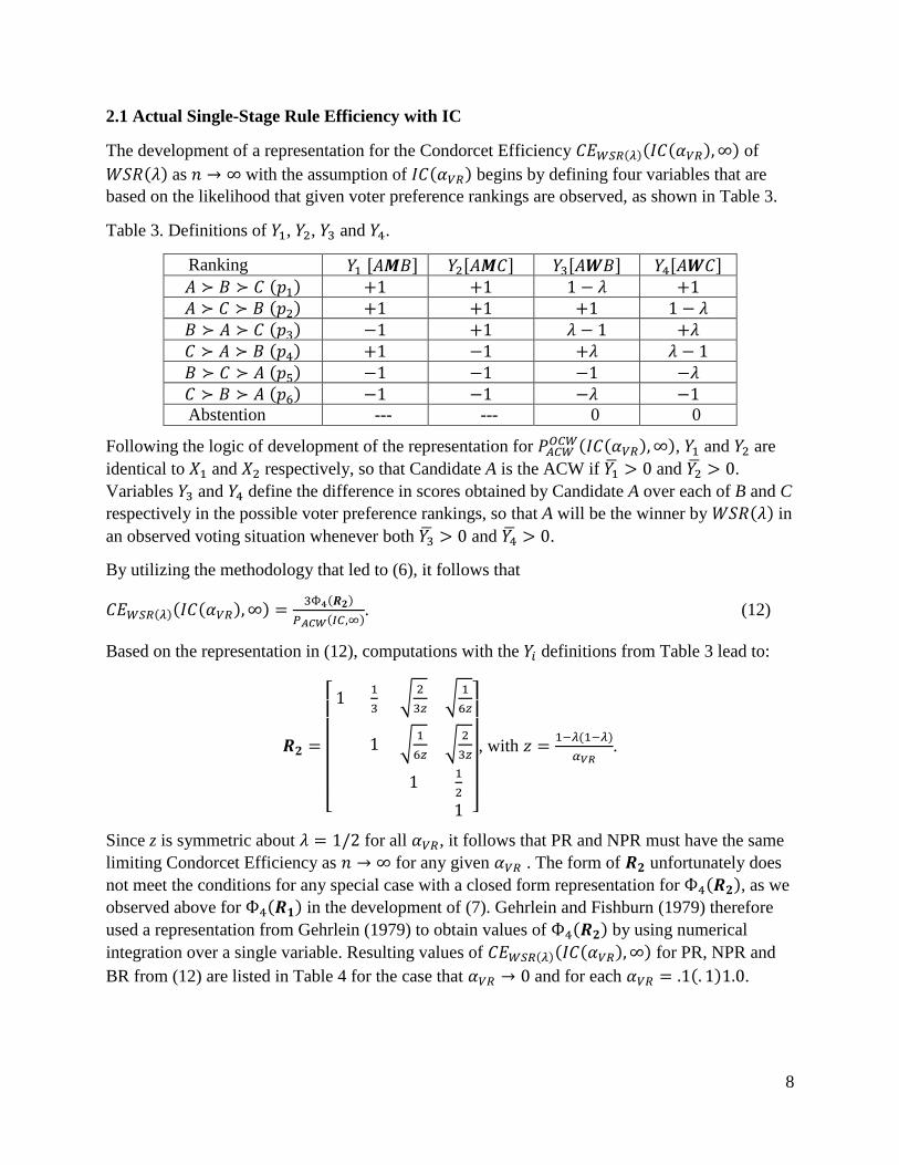
2.1 Actual Single-Stage Rule Efficiency with IC

The development of a representation for the Condorcet Efficiency 𝐶𝐸𝑊𝑆𝑅(𝜆)(𝐼𝐶(𝛼𝑉𝑅),∞) of

𝑊𝑆𝑅(𝜆) as 𝑛 → ∞ with the assumption of 𝐼𝐶(𝛼𝑉𝑅) begins by defining four variables that are

based on the likelihood that given voter preference rankings are observed, as shown in Table 3.

Table 3. Definitions of 𝑌1, 𝑌2, 𝑌3 and 𝑌4.

Ranking 𝑌1 [𝐴𝑴𝐵] 𝑌2[𝐴𝑴𝐶] 𝑌3[𝐴𝑾𝐵] 𝑌4[𝐴𝑾𝐶] 𝐴 ≻ 𝐵 ≻ 𝐶 (𝑝1) +1 +1 1 − 𝜆 +1

𝐴 ≻ 𝐶 ≻ 𝐵 (𝑝2) +1 +1 +1 1 − 𝜆

𝐵 ≻ 𝐴 ≻ 𝐶 (𝑝3) −1 +1 𝜆 − 1 +𝜆

𝐶 ≻ 𝐴 ≻ 𝐵 (𝑝4) +1 −1 +𝜆 𝜆 − 1

𝐵 ≻ 𝐶 ≻ 𝐴 (𝑝5) −1 −1 −1 −𝜆

𝐶 ≻ 𝐵 ≻ 𝐴 (𝑝6) −1 −1 −𝜆 −1

Abstention --- --- 0 0

Following the logic of development of the representation for 𝑃𝐴𝐶𝑊𝑂𝐶𝑊(𝐼𝐶(𝛼𝑉𝑅),∞), 𝑌1 and 𝑌2 are

identical to 𝑋1 and 𝑋2 respectively, so that Candidate A is the ACW if 𝑌1̅ > 0 and 𝑌2̅ > 0.

Variables 𝑌3 and 𝑌4 define the difference in scores obtained by Candidate A over each of B and C

respectively in the possible voter preference rankings, so that A will be the winner by 𝑊𝑆𝑅(𝜆) in

an observed voting situation whenever both 𝑌3̅ > 0 and 𝑌4̅ > 0.

By utilizing the methodology that led to (6), it follows that

𝐶𝐸𝑊𝑆𝑅(𝜆)(𝐼𝐶(𝛼𝑉𝑅),∞) =3Ф4(𝑹𝟐)

𝑃𝐴𝐶𝑊(𝐼𝐶,∞). (12)

Based on the representation in (12), computations with the 𝑌𝑖 definitions from Table 3 lead to:

𝑹𝟐 =

[ 1

1

3√

2

3𝑧√

1

6𝑧

1 √1

6𝑧√

2

3𝑧

11

2

1 ]

, with 𝑧 =1−𝜆(1−𝜆)

𝛼𝑉𝑅.

Since z is symmetric about 𝜆 = 1/2 for all 𝛼𝑉𝑅, it follows that PR and NPR must have the same

limiting Condorcet Efficiency as 𝑛 → ∞ for any given 𝛼𝑉𝑅 . The form of 𝑹𝟐 unfortunately does

not meet the conditions for any special case with a closed form representation for Ф4(𝑹𝟐), as we

observed above for Ф4(𝑹𝟏) in the development of (7). Gehrlein and Fishburn (1979) therefore

used a representation from Gehrlein (1979) to obtain values of Ф4(𝑹𝟐) by using numerical

integration over a single variable. Resulting values of 𝐶𝐸𝑊𝑆𝑅(𝜆)(𝐼𝐶(𝛼𝑉𝑅),∞) for PR, NPR and

BR from (12) are listed in Table 4 for the case that 𝛼𝑉𝑅 → 0 and for each 𝛼𝑉𝑅 = .1(. 1)1.0.

9

Table 4. Computed Limiting Values for Condorcet Efficiency with 𝐼𝐶(𝛼𝑉𝑅).

Voting Rule

𝛼𝑉𝑅 PR & NPR BR

≈ 0 1/3 = .3333 1/3 = .3333

.1 .4399 .4576

.2 .4882 .5151

.3 .5277 .5630

.4 .5630 .6068

.5 .5961 .6490

.6 .6280 .6911

.7 .6595 .7345

.8 .6911 .7810

.9 .7234 .8337

1.0 .7572 .9012

We see the expected result that Condorcet Efficiency values approach 1/3 to make all voting

rules equivalent to random selection procedures when 𝛼𝑉𝑅 → 0. We also note that BR dominates

PR and NPR for all non-zero participation rates. The efficiencies decrease rapidly as voter

participation rates decrease, and when this rate is 40% or less, all voting rules have Condorcet

Efficiency less than 61%. This level of efficiency is quite disappointing, since voter

participation rates as low as 40% are definitely observed in practice. For example, voter

participation rates in the 2014 US elections [see McDonald (2018) or other sources] range from

28.7% in Indiana to 58.7% in Maine, with an overall national participation rate of only 36.7%.

While these participation rates do increase for elections during years when a president is being

chosen, they are even lower during the primary elections to select final candidates. So, we

certainly hope that the introduction of a degree of dependence among voters’ preferences will

improve this situation.

2.2 Actual Single-Stage Rule Efficiency with IAC

The impact that the inclusion of some degree of dependence among voters’ preferences might

have on this dreary expected result is considered by using the assumption of 𝐼𝐴𝐶(𝛼𝑉𝑅) to obtain

representations for 𝐶𝐸𝑅𝑢𝑙𝑒(𝐼𝐴𝐶(𝛼𝑉𝑅),∞). It is not feasible to obtain such a representation for a

generalized 𝑊𝑆𝑅(𝜆) with a reasonable effort, as we did with 𝐶𝐸𝑊𝑆𝑅(𝜆)(𝐼𝐶(𝛼𝑉𝑅),∞), but we can

obtain a representation for each specified voting rule 𝑅𝑢𝑙𝑒 ∈ {𝑃𝑅,𝑁𝑃𝑅, 𝐵𝑅}.

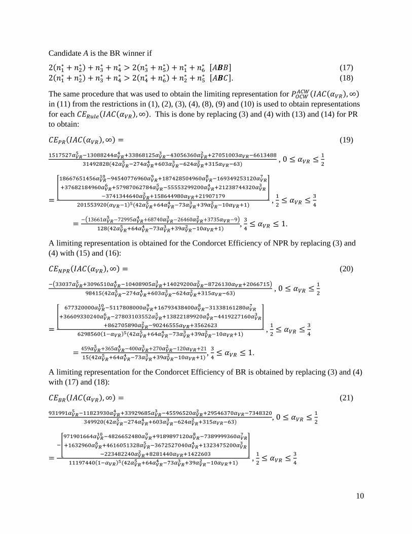
Based on the definitions of PR, NPR and BR that were given above, the following restrictions on

observed voting situations apply:

Candidate A is the PR winner if

𝑛1∗ + 𝑛2

∗ > 𝑛3∗ + 𝑛5

∗ [𝐴𝑷𝐵] (13)

𝑛1∗ + 𝑛2

∗ > 𝑛4∗ + 𝑛6

∗ [𝐴𝑷𝐶]. (14)

Candidate A is the NPR winner if

𝑛5∗ + 𝑛6

∗ < 𝑛2∗ + 𝑛4

∗ [𝐴𝑵𝐵] (15)

𝑛5∗ + 𝑛6

∗ < 𝑛1∗ + 𝑛3

∗ [𝐴𝑵𝐶]. (16)

10

Candidate A is the BR winner if

2(𝑛1∗ + 𝑛2

∗) + 𝑛3∗ + 𝑛4

∗ > 2(𝑛3∗ + 𝑛5

∗) + 𝑛1∗ + 𝑛6

∗ [𝐴𝑩𝐵] (17)

2(𝑛1∗ + 𝑛2

∗) + 𝑛3∗ + 𝑛4

∗ > 2(𝑛4∗ + 𝑛6

∗) + 𝑛2∗ + 𝑛5

∗ [𝐴𝑩𝐶]. (18)

The same procedure that was used to obtain the limiting representation for 𝑃𝑂𝐶𝑊𝐴𝐶𝑊(𝐼𝐴𝐶(𝛼𝑉𝑅),∞)

in (11) from the restrictions in (1), (2), (3), (4), (8), (9) and (10) is used to obtain representations

for each 𝐶𝐸𝑅𝑢𝑙𝑒(𝐼𝐴𝐶(𝛼𝑉𝑅),∞). This is done by replacing (3) and (4) with (13) and (14) for PR

to obtain:

𝐶𝐸𝑃𝑅(𝐼𝐴𝐶(𝛼𝑉𝑅),∞) = (19)

1517527𝛼𝑉𝑅5 −13088244𝛼𝑉𝑅

4 +33868125𝛼𝑉𝑅3 −43056360𝛼𝑉𝑅

2 +27051003𝛼𝑉𝑅−6613488

31492828(42𝛼𝑉𝑅5 −274𝛼𝑉𝑅

4 +603𝛼𝑉𝑅3 −624𝛼𝑉𝑅

2 +315𝛼𝑉𝑅−63) , 0 ≤ 𝛼𝑉𝑅 ≤

1

2

=

[

18667651456𝛼𝑉𝑅10 −94540776960𝛼𝑉𝑅

9 +187428504960𝛼𝑉𝑅8 −169349253120𝛼𝑉𝑅

7

+37682184960𝛼𝑉𝑅6 +57987062784𝛼𝑉𝑅

5 −55553299200𝛼𝑉𝑅4 +21238744320𝛼𝑉𝑅

3

−3741344640𝛼𝑉𝑅2 +158644980𝛼𝑉𝑅+21907179

]

201553920(𝛼𝑉𝑅−1)5(42𝛼𝑉𝑅5 +64𝛼𝑉𝑅

4 −73𝛼𝑉𝑅3 +39𝛼𝑉𝑅

2 −10𝛼𝑉𝑅+1) ,

1

2≤ 𝛼𝑉𝑅 ≤

3

4

=−(13661𝛼𝑉𝑅

5 −72995𝛼𝑉𝑅4 +68740𝛼𝑉𝑅

3 −26460𝛼𝑉𝑅2 +3735𝛼𝑉𝑅−9)

128(42𝛼𝑉𝑅5 +64𝛼𝑉𝑅

4 −73𝛼𝑉𝑅3 +39𝛼𝑉𝑅

2 −10𝛼𝑉𝑅+1),

3

4≤ 𝛼𝑉𝑅 ≤ 1.

A limiting representation is obtained for the Condorcet Efficiency of NPR by replacing (3) and

(4) with (15) and (16):

𝐶𝐸𝑁𝑃𝑅(𝐼𝐴𝐶(𝛼𝑉𝑅),∞) = (20)

−(33037𝛼𝑉𝑅5 +3096510𝛼𝑉𝑅

4 −10408905𝛼𝑉𝑅3 +14029200𝛼𝑉𝑅

2 −8726130𝛼𝑉𝑅+2066715)

98415(42𝛼𝑉𝑅5 −274𝛼𝑉𝑅

4 +603𝛼𝑉𝑅3 −624𝛼𝑉𝑅

2 +315𝛼𝑉𝑅−63) , 0 ≤ 𝛼𝑉𝑅 ≤

1

2

=

[

677320000𝛼𝑉𝑅10 −5117808000𝛼𝑉𝑅

9 +16793438400𝛼𝑉𝑅8 −31338161280𝛼𝑉𝑅

7

+36609330240𝛼𝑉𝑅6 −27803103552𝛼𝑉𝑅

5 +13822189920𝛼𝑉𝑅4 −4419227160𝛼𝑉𝑅

3

+862705890𝛼𝑉𝑅2 −90246555𝛼𝑉𝑅+3562623

]

6298560(1−𝛼𝑉𝑅)5(42𝛼𝑉𝑅5 +64𝛼𝑉𝑅

4 −73𝛼𝑉𝑅3 +39𝛼𝑉𝑅

2 −10𝛼𝑉𝑅+1) ,

1

2≤ 𝛼𝑉𝑅 ≤

3

4

=459𝛼𝑉𝑅

5 +365𝛼𝑉𝑅4 −400𝛼𝑉𝑅

3 +270𝛼𝑉𝑅2 −120𝛼𝑉𝑅+21

15(42𝛼𝑉𝑅5 +64𝛼𝑉𝑅

4 −73𝛼𝑉𝑅3 +39𝛼𝑉𝑅

2 −10𝛼𝑉𝑅+1),

3

4≤ 𝛼𝑉𝑅 ≤ 1.

A limiting representation for the Condorcet Efficiency of BR is obtained by replacing (3) and (4)

with (17) and (18):

𝐶𝐸𝐵𝑅(𝐼𝐴𝐶(𝛼𝑉𝑅),∞) = (21)

931991𝛼𝑉𝑅5 −11823930𝛼𝑉𝑅

4 +33929685𝛼𝑉𝑅3 −45596520𝛼𝑉𝑅

2 +29546370𝛼𝑉𝑅−7348320

349920(42𝛼𝑉𝑅5 −274𝛼𝑉𝑅

4 +603𝛼𝑉𝑅3 −624𝛼𝑉𝑅

2 +315𝛼𝑉𝑅−63), 0 ≤ 𝛼𝑉𝑅 ≤

1

2

=

−[

971901664𝛼𝑉𝑅10 −4826652480𝛼𝑉𝑅

9 +9189897120𝛼𝑉𝑅8 −7389999360𝛼𝑉𝑅

7

+1632960𝛼𝑉𝑅6 +4616051328𝛼𝑉𝑅

5 −3672527040𝛼𝑉𝑅4 +1323475200𝛼𝑉𝑅

3

−223482240𝛼𝑉𝑅2 +8281440𝛼𝑉𝑅+1422603

]

11197440(1−𝛼𝑉𝑅)5(42𝛼𝑉𝑅5 +64𝛼𝑉𝑅

4 −73𝛼𝑉𝑅3 +39𝛼𝑉𝑅

2 −10𝛼𝑉𝑅+1) ,

1

2≤ 𝛼𝑉𝑅 ≤

3

4

11

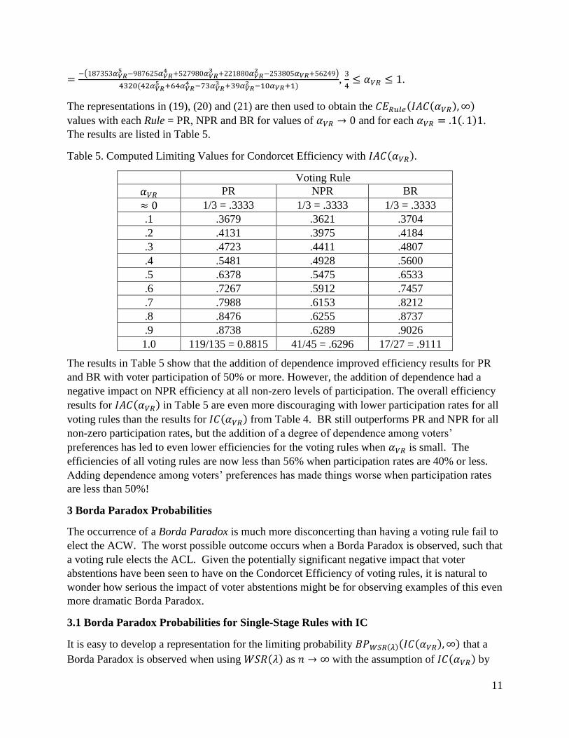
=−(187353𝛼𝑉𝑅

5 −987625𝛼𝑉𝑅4 +527980𝛼𝑉𝑅

3 +221880𝛼𝑉𝑅2 −253805𝛼𝑉𝑅+56249)

4320(42𝛼𝑉𝑅5 +64𝛼𝑉𝑅

4 −73𝛼𝑉𝑅3 +39𝛼𝑉𝑅

2 −10𝛼𝑉𝑅+1),

3

4≤ 𝛼𝑉𝑅 ≤ 1.

The representations in (19), (20) and (21) are then used to obtain the 𝐶𝐸𝑅𝑢𝑙𝑒(𝐼𝐴𝐶(𝛼𝑉𝑅),∞)

values with each Rule = PR, NPR and BR for values of 𝛼𝑉𝑅 → 0 and for each 𝛼𝑉𝑅 = .1(. 1)1.

The results are listed in Table 5.

Table 5. Computed Limiting Values for Condorcet Efficiency with 𝐼𝐴𝐶(𝛼𝑉𝑅).

Voting Rule

𝛼𝑉𝑅 PR NPR BR

≈ 0 1/3 = .3333 1/3 = .3333 1/3 = .3333

.1 .3679 .3621 .3704

.2 .4131 .3975 .4184

.3 .4723 .4411 .4807

.4 .5481 .4928 .5600

.5 .6378 .5475 .6533

.6 .7267 .5912 .7457

.7 .7988 .6153 .8212

.8 .8476 .6255 .8737

.9 .8738 .6289 .9026

1.0 119/135 = 0.8815 41/45 = .6296 17/27 = .9111

The results in Table 5 show that the addition of dependence improved efficiency results for PR

and BR with voter participation of 50% or more. However, the addition of dependence had a

negative impact on NPR efficiency at all non-zero levels of participation. The overall efficiency

results for 𝐼𝐴𝐶(𝛼𝑉𝑅) in Table 5 are even more discouraging with lower participation rates for all

voting rules than the results for 𝐼𝐶(𝛼𝑉𝑅) from Table 4. BR still outperforms PR and NPR for all

non-zero participation rates, but the addition of a degree of dependence among voters’

preferences has led to even lower efficiencies for the voting rules when 𝛼𝑉𝑅 is small. The

efficiencies of all voting rules are now less than 56% when participation rates are 40% or less.

Adding dependence among voters’ preferences has made things worse when participation rates

are less than 50%!

3 Borda Paradox Probabilities

The occurrence of a Borda Paradox is much more disconcerting than having a voting rule fail to

elect the ACW. The worst possible outcome occurs when a Borda Paradox is observed, such that

a voting rule elects the ACL. Given the potentially significant negative impact that voter

abstentions have been seen to have on the Condorcet Efficiency of voting rules, it is natural to

wonder how serious the impact of voter abstentions might be for observing examples of this even

more dramatic Borda Paradox.

3.1 Borda Paradox Probabilities for Single-Stage Rules with IC

It is easy to develop a representation for the limiting probability 𝐵𝑃𝑊𝑆𝑅(𝜆)(𝐼𝐶(𝛼𝑉𝑅),∞) that a

Borda Paradox is observed when using 𝑊𝑆𝑅(𝜆) as 𝑛 → ∞ with the assumption of 𝐼𝐶(𝛼𝑉𝑅) by

12

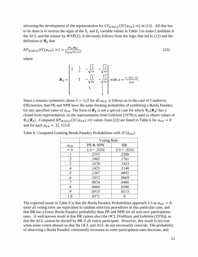
mirroring the development of the representation for 𝐶𝐸𝑊𝑆𝑅(𝜆)(𝐼𝐶(𝛼𝑉𝑅),∞) in (12). All that has

to be done is to reverse the signs of the 𝑌1 and 𝑌2 variable values in Table 3 to make Candidate A

the ACL and the winner by 𝑊𝑆𝑅(𝜆). It obviously follows from the logic that led to (12) and the

definition of 𝑹𝟐 that

𝐵𝑃𝑊𝑆𝑅(𝜆)(𝐼𝐶(𝛼𝑉𝑅),∞) =3Ф4(𝑹𝟑)

𝑃𝐴𝐶𝑊(𝐼𝐶,∞), (22)

where

𝑹𝟑 =

[ 1

1

3−√

2

3𝑧−√

1

6𝑧

1 −√1

6𝑧−√

2

3𝑧

11

2

1 ]

, with 𝑧 =1−𝜆(1−𝜆)

𝛼𝑉𝑅.

Since z remains symmetric about 𝜆 = 1/2 for all 𝛼𝑉𝑅, it follows as in the case of Condorcet

Efficiencies, that PR and NPR have the same limiting probability of exhibiting a Borda Paradox

for any specified value of 𝛼𝑉𝑅. The form of 𝑹𝟑 is not a special case for which Ф4(𝑹𝟑) has a

closed form representation, so the representation from Gehrlein (1979) is used to obtain values of

Ф4(𝑹𝟑). Computed 𝐵𝑃𝑊𝑆𝑅(𝜆)(𝐼𝐶(𝛼𝑉𝑅),∞) values from (22) are listed in Table 6 for 𝛼𝑉𝑅 → 0

and for each 𝛼𝑉𝑅 = .1(. 1)1.0

Table 6. Computed Limiting Borda Paradox Probabilities with 𝐼𝐶(𝛼𝑉𝑅).

Voting Rule

𝛼𝑉𝑅 PR & NPR BR

≈ 0 1/3 = .3333 1/3 = .3333

.1 .2355 .2208

.2 .1965 .1761

.3 .1670 .1423

.4 .1423 .1140

.5 .1207 .0892

.6 .1012 .0669

.7 .0834 .0466

.8 .0669 .0280

.9 .0515 .0115

1.0 .0371 0

The expected result in Table 6 is that the Borda Paradox Probabilities approach 1/3 as 𝛼𝑉𝑅 → 0,

since all voting rules are equivalent to random selection procedures in this particular case, and

that BR has a lower Borda Paradox probability than PR and NPR for all non-zero participation

rates. A well-known result is that BR cannot elect the OCL [Fishburn and Gehrlein (1976)], so

that the ACL cannot be elected by BR if all voters participate. However, this result is not true

when some voters abstain so that the OCL and ACL do not necessarily coincide. The probability

of observing a Borda Paradox consistently increases as voter participation rates decrease, and

13

when this rate is 40% or less, all voting rules have a Borda Paradox probability of greater than

11%! That is a shockingly large probability for such a very negative outcome, given that voter

participation rates as low as 40% are actually observed in practice.

3.2 Borda Paradox Probabilities for Single-Stage Rules with IAC

We consider the impact that the introduction of some degree of dependence among voters’

preferences will have on the probability that Borda’s Paradox will be observed by extending this

analysis with the assumption of 𝐼𝐴𝐶(𝛼𝑉𝑅). This begins by noting that Candidate A is the ACL

whenever:

𝑛3 + 𝑛5 + 𝑛6 > 𝑛1 + 𝑛2 + 𝑛4 [𝐵𝑴𝐴] (23)

𝑛4 + 𝑛5 + 𝑛6 > 𝑛1 + 𝑛2 + 𝑛3 [𝐶𝑴𝐴]. (24)

The representation for 𝐶𝐸𝑃𝑅(𝐼𝐴𝐶(𝛼𝑉𝑅),∞) in (19) was obtained by considering actual and

observed voting situations for which (1), (2), (13), (14), (8), (9) and (10) held simultaneously.

Here, (1) and (2) respectively required that AMB and AMC to make Candidate A the ACW. This

process is then repeated by replacing (1) and (2) with (23) and (24) to obtain a representation for

𝐵𝑃𝑃𝑅(𝐼𝐴𝐶(𝛼𝑉𝑅),∞), with

𝐵𝑃𝑃𝑅(𝐼𝐴𝐶(𝛼𝑉𝑅),∞) = (25) 58215686𝛼𝑉𝑅

5 − 284362350𝛼𝑉𝑅4 + 519458670𝛼𝑉𝑅

3 − 455939280𝛼𝑉𝑅2 + 195419385𝛼𝑉𝑅 − 33067440

1574640(42𝛼𝑉𝑅5 − 274𝛼𝑉𝑅

4 + 603𝛼𝑉𝑅3 − 624𝛼𝑉𝑅

2 + 315𝛼𝑉𝑅 − 63)’

0 ≤ 𝛼𝑉𝑅 ≤1

2.

[1687165696𝛼𝑉𝑅

10 −10095594240𝛼𝑉𝑅9 +23635307520𝛼𝑉𝑅

8 −22382853120𝛼𝑉𝑅7 −8582837760𝛼𝑉𝑅

6 +

45924060672𝛼𝑉𝑅5 −53966062080𝛼𝑉𝑅

4 +33709893120𝛼𝑉𝑅3 −12060167760𝛼𝑉𝑅

2 +2317476420𝛼𝑉𝑅−186417693]

201553920(𝛼𝑉𝑅−1)5 (42𝛼𝑉𝑅5 +64𝛼𝑉𝑅

4 −73𝛼𝑉𝑅3 +39𝛼𝑉𝑅

2 −10𝛼𝑉𝑅+1),

1

2≤ 𝛼𝑉𝑅 ≤

3

4

−(1989𝛼𝑉𝑅5 −9340𝛼𝑉𝑅

4 +14390𝛼𝑉𝑅3 −9900𝛼𝑉𝑅

2 +2925𝛼𝑉𝑅−288)

120(42𝛼𝑉𝑅5 +64𝛼𝑉𝑅

4 −73𝛼𝑉𝑅3 +39𝛼𝑉𝑅

2 −10𝛼𝑉𝑅+1),

3

4≤ 𝛼𝑉𝑅 ≤ 1.

This process is then repeated for both NPR and BR, and the resulting limiting representations for

observing Borda’s Paradox are given by:

𝐵𝑃𝑁𝑃𝑅(𝐼𝐴𝐶(𝛼𝑉𝑅),∞) = (26)

2571059𝛼𝑉𝑅5 −14546670𝛼𝑉𝑅

4 +28993545𝛼𝑉𝑅3 −26888760𝛼𝑉𝑅

2 +11941020𝛼𝑉𝑅−2066715

98415(42𝛼𝑉𝑅5 −274𝛼𝑉𝑅

4 +603𝛼𝑉𝑅3 −624𝛼𝑉𝑅

2 +315𝛼𝑉𝑅−63), 0 ≤ 𝛼𝑉𝑅 ≤

1

2

[198413056𝛼𝑉𝑅

10 −1667619840𝛼𝑉𝑅9 +6862786560𝛼𝑉𝑅

8 −17302947840𝛼𝑉𝑅7 +28555571520𝛼𝑉𝑅

6

−31612472640𝛼𝑉𝑅5 +23544017280𝛼𝑉𝑅

4 −11583051840𝛼𝑉𝑅3 +3587226750𝛼𝑉𝑅

2 −629659170𝛼𝑉𝑅+47731275]

25194240(1−𝛼𝑉𝑅)5(42𝛼𝑉𝑅5 +64𝛼𝑉𝑅

4 −73𝛼𝑉𝑅3 +39𝛼𝑉𝑅

2 −10𝛼𝑉𝑅+1),

for 1

2≤ 𝛼𝑉𝑅 ≤

3

4

340𝛼𝑉𝑅5 +20𝛼𝑉𝑅

4 −1060𝛼𝑉𝑅3 +1260𝛼𝑉𝑅

2 −525𝛼𝑉𝑅+84

60(42𝛼𝑉𝑅5 +64𝛼𝑉𝑅

4 −73𝛼𝑉𝑅3 +39𝛼𝑉𝑅

2 −10𝛼𝑉𝑅+1), for 3

4≤ 𝛼𝑉𝑅 ≤ 1.

14

𝐵𝑃𝐵𝑅(𝐼𝐴𝐶(𝛼𝑉𝑅),∞) = (27)

2603797𝛼𝑉𝑅5 −12826098𝛼𝑉𝑅

4 +23528961𝛼𝑉𝑅3 −20631672𝛼𝑉𝑅

2 +8787366𝛼𝑉𝑅−1469664

69984(42𝛼𝑉𝑅5 −274𝛼𝑉𝑅

4 +603𝛼𝑉𝑅3 −624𝛼𝑉𝑅

2 +315𝛼𝑉𝑅−63), 0 ≤ 𝛼𝑉𝑅 ≤

1

2

[37038752𝛼𝑉𝑅

10 −252012096𝛼𝑉𝑅9 +721014048𝛼𝑉𝑅

8 −1093927680𝛼𝑉𝑅7 +868408128𝛼𝑉𝑅

6 −

191382912𝛼𝑉𝑅5 −275970240𝛼𝑉𝑅

4 +284850432𝛼𝑉𝑅3 −121223952𝛼𝑉𝑅

2 +25345872𝛼𝑉𝑅−2140425]

2239488(𝛼𝑉𝑅−1)5(42𝛼𝑉𝑅5 +64𝛼𝑉𝑅

4 −73𝛼𝑉𝑅3 +39𝛼𝑉𝑅

2 −10𝛼𝑉𝑅+1), 1

2≤ 𝛼𝑉𝑅 ≤

3

4

(1−𝛼𝑉𝑅)3(99387𝛼𝑉𝑅2 −94358𝛼𝑉𝑅+24131)

864(42𝛼𝑉𝑅5 +64𝛼𝑉𝑅

4 −73𝛼𝑉𝑅3 +39𝛼𝑉𝑅

2 −10𝛼𝑉𝑅+1), 3

4≤ 𝛼𝑉𝑅 ≤ 1.

Associated values of 𝐵𝑃𝑃𝑅(𝐼𝐴𝐶(𝛼𝑉𝑅),∞) from (25), 𝐵𝑃𝑁𝑃𝑅(𝐼𝐴𝐶(𝛼𝑉𝑅),∞) from (26) and

𝐵𝑃𝐵𝑅(𝐼𝐴𝐶(𝛼𝑉𝑅),∞) from (27) are listed in Table 7 for 𝛼𝑉𝑅 → 0 and for each 𝛼𝑉𝑅 = .1(. 1)1.0.

Table 7. Computed Limiting Borda Paradox Probabilities with 𝐼𝐴𝐶(𝛼𝑉𝑅).

Voting Rule

𝛼𝑉𝑅 PR NPR BR

≈ 0 1/3 = .3333 1/3 = .3333 1/3 = .3333

.1 .3006 .3046 .2980

.2 .2626 .2691 .2564

.3 .2186 .2257 .2077

.4 .1693 .1745 .1526

.5 .1192 .1207 .0962

.6 .0778 .0773 .0497

.7 .0508 .0512 .0202

.8 .0366 .0383 .0055

.9 .0309 .0328 .0006

1.0 4/135=.0296 17/540=.0315 0

A comparison of the results in Tables 6 and 7 shows the same general outcome that was

observed when the Condorcet Efficiency of voting rules was analyzed earlier with 𝐼𝐶(𝛼𝑉𝑅) and

𝐼𝐴𝐶(𝛼𝑉𝑅). That is, the addition of a degree of dependence among voters’ preferences with

𝐼𝐴𝐶(𝛼𝑉𝑅) actually makes things worse for lower levels of voter participation. We now see that

the probability of observing a Borda Paradox is greater than 15% for all levels of voter

participation at 40% or less! The results for BR are uniformly the best of these options for all

positive levels of voter participation, but BR still performs very poorly for lower levels of voter

participation. If this very poor overall performance of single-stage voting rules at lower levels of

voter participation is to be improved, the likely approach would be to consider the use of some

other forms of voting rules.

4 Two-stage Voting Rules

Two-stage voting rules are sequential elimination procedures that take place in two steps. In the

first stage, a voting rule is used to determine the candidate that is ranked as the worst of the three

candidates. That candidate is eliminated from consideration in the second stage, where majority

rule is used to determine the ultimate winner from the remaining two candidates. All that

changes with the two-stage rules is the voting rule that is used to eliminate the loser in the first

15

stage. We consider Plurality Elimination Rule (PER), Negative Plurality Elimination Rule

(NPER) and Borda Elimination Rule (BER). It is definitely of interest to determine if these two-

stage voting rules can exhibit better performance than the single-stage rules on the basis of

Condorcet Efficiency and the probability that Borda’s Paradox is observed with lower levels of

voter participation rates.

4.1 Condorcet Efficiency of Two-stage Voting Rules with IC

The development of the representation for 𝐶𝐸𝑊𝑆𝑅(𝜆)(𝐼𝐶(𝛼𝑉𝑅),∞) in (12) was based on the

definitions of the four 𝑌𝑖 variables in Table 3 had 𝑌�̅� > 0 for 𝑖 = 1,2,3,4. When we consider

instead the more complex two-stage elimination rules 𝑊𝑆𝑅𝐸(𝜆), the resulting development of a

representation for 𝐶𝐸𝑊𝑆𝑅𝐸(𝜆)(𝐼𝐶(𝛼𝑉𝑅),∞) requires the use of five variables that are denoted as

𝑍𝑖 for 𝑖 = 1,2,3,4,5 in Table 8.

Table 8. Definitions of 𝑍1, 𝑍2, 𝑍3, 𝑍4 and 𝑍5.

Ranking 𝑍1 [𝐴𝑴𝐵] 𝑍2[𝐴𝑴𝐶] 𝑍3[𝐴𝑾𝐵] 𝑍4[𝐶𝑾𝐵] 𝑍5[𝐴𝑴∗𝐶]

𝐴 ≻ 𝐵 ≻ 𝐶 (𝑝1) +1 +1 1 − 𝜆 −𝜆 +1𝐴 ≻ 𝐶 ≻ 𝐵 (𝑝2) +1 +1 +1 𝜆 +1𝐵 ≻ 𝐴 ≻ 𝐶 (𝑝3) −1 +1 𝜆 − 1 −1 +1𝐶 ≻ 𝐴 ≻ 𝐵 (𝑝4) +1 −1 𝜆 +1 −1𝐵 ≻ 𝐶 ≻ 𝐴 (𝑝5) −1 −1 −1 𝜆 − 1 −1𝐶 ≻ 𝐵 ≻ 𝐴 (𝑝6) −1 −1 −𝜆 1 − 𝜆 −1

Abstention --- --- 0 0 0

By comparing Table 8 to Table 3, we see that 𝑍1 and 𝑍2 are identical to 𝑌1 and 𝑌2, so that

Candidate A will be the ACW if �̅�1 > 0 and �̅�2 > 0. It is also true that 𝑍3 is identical to 𝑌3, so

that A beats B by 𝑊𝑆𝑅(𝜆) if �̅�3 > 0. Variable 𝑍4 defines the relative margin by which C beats B

in each ranking under 𝑊𝑆𝑅(𝜆). So, B will be the lowest ranked candidate by 𝑊𝑆𝑅(𝜆) when

�̅�3 > 0 and �̅�4 > 0, and it therefore will be eliminated under 𝑊𝑆𝑅𝐸(𝜆). Variable 𝑍5 accounts

for the fact that the ACW Candidate A will then be the majority rule winner over C for

participating voters in the second stage of 𝑊𝑆𝑅𝐸(𝜆) if �̅�5 > 0. Candidate A will therefore be the

ACW and the winner by 𝑊𝑆𝑅𝐸(𝜆) when �̅�𝑖 > 0 for 𝑖 = 1,2,3,4,5.

The correlation matrix between these five variables is found to be given by 𝑹𝟓:

𝑹𝟓 =

[

11

3√

2

3𝑧√

1

6𝑧

√𝛼𝑉𝑅

3

1 √1

6𝑧−√

1

6𝑧√𝛼𝑉𝑅

11

2√

1

6𝑧𝛼𝑉𝑅

1 −√1

6𝑧𝛼𝑉𝑅

1 ]

, with 𝑧 =1−𝜆(1−𝜆)

𝛼𝑉𝑅.

16

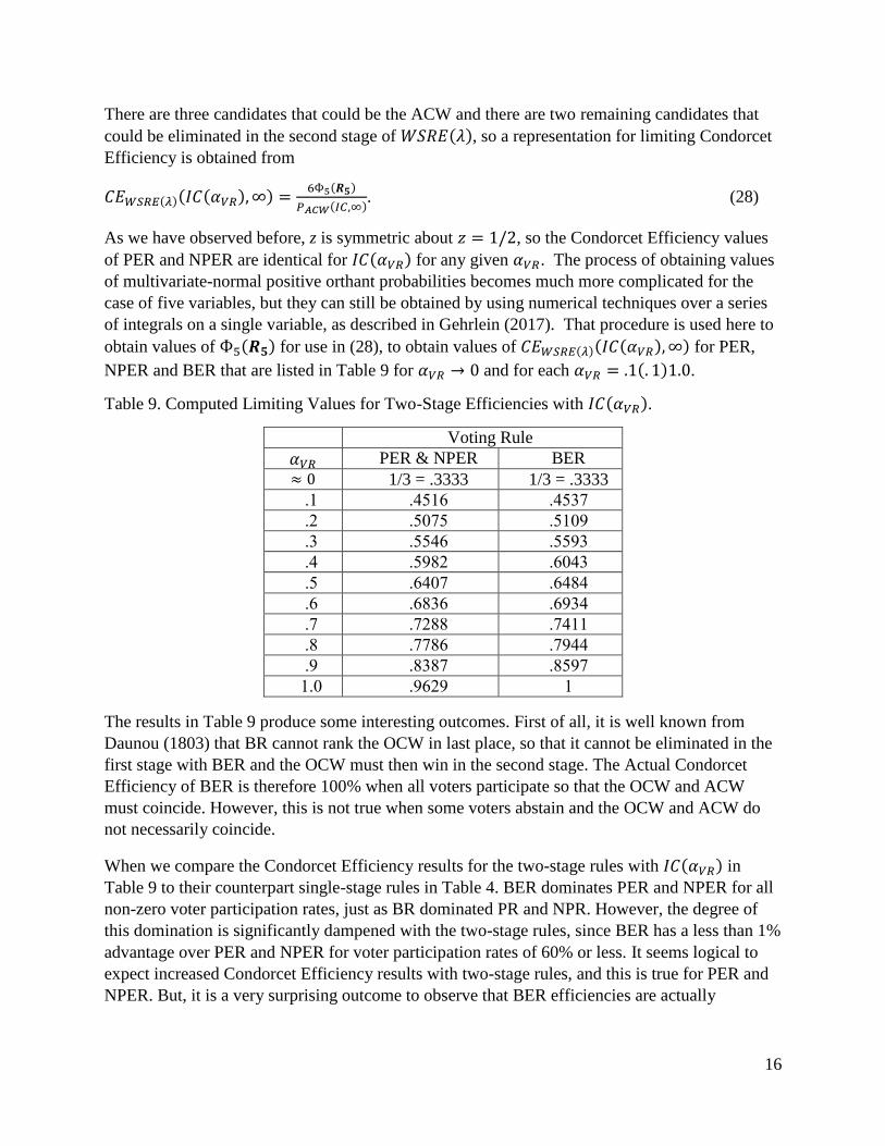
There are three candidates that could be the ACW and there are two remaining candidates that

could be eliminated in the second stage of 𝑊𝑆𝑅𝐸(𝜆), so a representation for limiting Condorcet

Efficiency is obtained from

𝐶𝐸𝑊𝑆𝑅𝐸(𝜆)(𝐼𝐶(𝛼𝑉𝑅),∞) =6Ф5(𝑹𝟓)

𝑃𝐴𝐶𝑊(𝐼𝐶,∞). (28)

As we have observed before, z is symmetric about 𝑧 = 1/2, so the Condorcet Efficiency values

of PER and NPER are identical for 𝐼𝐶(𝛼𝑉𝑅) for any given 𝛼𝑉𝑅. The process of obtaining values

of multivariate-normal positive orthant probabilities becomes much more complicated for the

case of five variables, but they can still be obtained by using numerical techniques over a series

of integrals on a single variable, as described in Gehrlein (2017). That procedure is used here to

obtain values of Ф5(𝑹𝟓) for use in (28), to obtain values of 𝐶𝐸𝑊𝑆𝑅𝐸(𝜆)(𝐼𝐶(𝛼𝑉𝑅),∞) for PER,

NPER and BER that are listed in Table 9 for 𝛼𝑉𝑅 → 0 and for each 𝛼𝑉𝑅 = .1(. 1)1.0.

Table 9. Computed Limiting Values for Two-Stage Efficiencies with 𝐼𝐶(𝛼𝑉𝑅).

Voting Rule

𝛼𝑉𝑅 PER & NPER BER

≈ 0 1/3 = .3333 1/3 = .3333

.1 .4516 .4537

.2 .5075 .5109

.3 .5546 .5593

.4 .5982 .6043

.5 .6407 .6484

.6 .6836 .6934

.7 .7288 .7411

.8 .7786 .7944

.9 .8387 .8597

1.0 .9629 1

The results in Table 9 produce some interesting outcomes. First of all, it is well known from

Daunou (1803) that BR cannot rank the OCW in last place, so that it cannot be eliminated in the

first stage with BER and the OCW must then win in the second stage. The Actual Condorcet

Efficiency of BER is therefore 100% when all voters participate so that the OCW and ACW

must coincide. However, this is not true when some voters abstain and the OCW and ACW do

not necessarily coincide.

When we compare the Condorcet Efficiency results for the two-stage rules with 𝐼𝐶(𝛼𝑉𝑅) in

Table 9 to their counterpart single-stage rules in Table 4. BER dominates PER and NPER for all

non-zero voter participation rates, just as BR dominated PR and NPR. However, the degree of

this domination is significantly dampened with the two-stage rules, since BER has a less than 1%

advantage over PER and NPER for voter participation rates of 60% or less. It seems logical to

expect increased Condorcet Efficiency results with two-stage rules, and this is true for PER and

NPER. But, it is a very surprising outcome to observe that BER efficiencies are actually

17

marginally smaller than BR efficiencies for . 1 ≤ 𝛼𝑉𝑅 ≤ .5 and the Condorcet Efficiency values

for two-stage rules remain less than 61% for voter participation rates that are 40% or less.

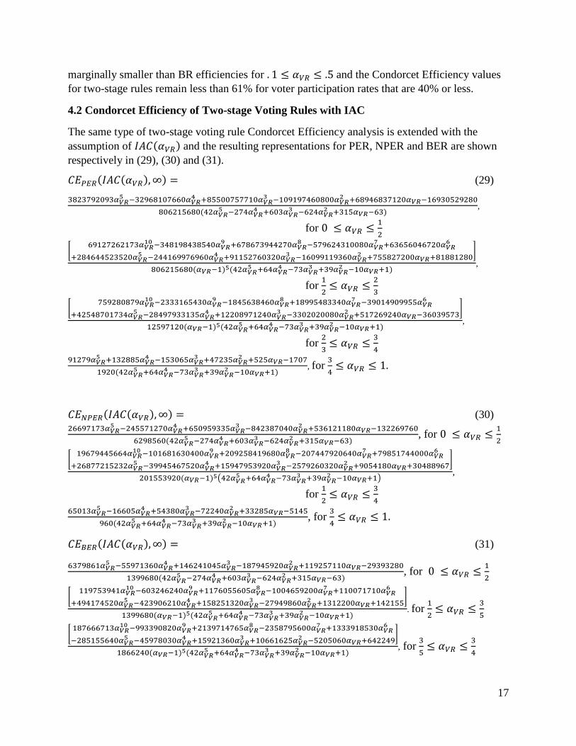
4.2 Condorcet Efficiency of Two-stage Voting Rules with IAC

The same type of two-stage voting rule Condorcet Efficiency analysis is extended with the

assumption of 𝐼𝐴𝐶(𝛼𝑉𝑅) and the resulting representations for PER, NPER and BER are shown

respectively in (29), (30) and (31).

𝐶𝐸𝑃𝐸𝑅(𝐼𝐴𝐶(𝛼𝑉𝑅),∞) = (29)

3823792093𝛼𝑉𝑅5 −32968107660𝛼𝑉𝑅

4 +85500757710𝛼𝑉𝑅3 −109197460800𝛼𝑉𝑅

2 +68946837120𝛼𝑉𝑅−16930529280

806215680(42𝛼𝑉𝑅5 −274𝛼𝑉𝑅

4 +603𝛼𝑉𝑅3 −624𝛼𝑉𝑅

2 +315𝛼𝑉𝑅−63),

for 0 ≤ 𝛼𝑉𝑅 ≤1

2

[69127262173𝛼𝑉𝑅

10 −348198438540𝛼𝑉𝑅9 +678673944270𝛼𝑉𝑅

8 −579624310080𝛼𝑉𝑅7 +63656046720𝛼𝑉𝑅

6

+284644523520𝛼𝑉𝑅5 −244169976960𝛼𝑉𝑅

4 +91152760320𝛼𝑉𝑅3 −16099119360𝛼𝑉𝑅

2 +755827200𝛼𝑉𝑅+81881280]

806215680(𝛼𝑉𝑅−1)5(42𝛼𝑉𝑅5 +64𝛼𝑉𝑅

4 −73𝛼𝑉𝑅3 +39𝛼𝑉𝑅

2 −10𝛼𝑉𝑅+1),

for 1

2≤ 𝛼𝑉𝑅 ≤

2

3

[759280879𝛼𝑉𝑅

10 −2333165430𝛼𝑉𝑅9 −1845638460𝛼𝑉𝑅

8 +18995483340𝛼𝑉𝑅7 −39014909955𝛼𝑉𝑅

6

+42548701734𝛼𝑉𝑅5 −28497933135𝛼𝑉𝑅

4 +12208971240𝛼𝑉𝑅3 −3302020080𝛼𝑉𝑅

2 +517269240𝛼𝑉𝑅−36039573]

12597120(𝛼𝑉𝑅−1)5(42𝛼𝑉𝑅5 +64𝛼𝑉𝑅

4 −73𝛼𝑉𝑅3 +39𝛼𝑉𝑅

2 −10𝛼𝑉𝑅+1),

for 2

3≤ 𝛼𝑉𝑅 ≤

3

4

91279𝛼𝑉𝑅5 +132885𝛼𝑉𝑅

4 −153065𝛼𝑉𝑅3 +47235𝛼𝑉𝑅

2 +525𝛼𝑉𝑅−1707

1920(42𝛼𝑉𝑅5 +64𝛼𝑉𝑅

4 −73𝛼𝑉𝑅3 +39𝛼𝑉𝑅

2 −10𝛼𝑉𝑅+1), for

3

4≤ 𝛼𝑉𝑅 ≤ 1.

𝐶𝐸𝑁𝑃𝐸𝑅(𝐼𝐴𝐶(𝛼𝑉𝑅),∞) = (30)

26697173𝛼𝑉𝑅5 −245571270𝛼𝑉𝑅

4 +650959335𝛼𝑉𝑅3 −842387040𝛼𝑉𝑅

2 +536121180𝛼𝑉𝑅−132269760

6298560(42𝛼𝑉𝑅5 −274𝛼𝑉𝑅

4 +603𝛼𝑉𝑅3 −624𝛼𝑉𝑅

2 +315𝛼𝑉𝑅−63), for 0 ≤ 𝛼𝑉𝑅 ≤

1

2

[19679445664𝛼𝑉𝑅

10 −101681630400𝛼𝑉𝑅9 +209258419680𝛼𝑉𝑅

8 −207447920640𝛼𝑉𝑅7 +79851744000𝛼𝑉𝑅

6

+26877215232𝛼𝑉𝑅5 −39945467520𝛼𝑉𝑅

4 +15947953920𝛼𝑉𝑅3 −2579260320𝛼𝑉𝑅

2 +9054180𝛼𝑉𝑅+30488967]

201553920(𝛼𝑉𝑅−1)5(42𝛼𝑉𝑅5 +64𝛼𝑉𝑅

4 −73𝛼𝑉𝑅3 +39𝛼𝑉𝑅

2 −10𝛼𝑉𝑅+1),

for 1

2≤ 𝛼𝑉𝑅 ≤

3

4

65013𝛼𝑉𝑅5 −16605𝛼𝑉𝑅

4 +54380𝛼𝑉𝑅3 −72240𝛼𝑉𝑅

2 +33285𝛼𝑉𝑅−5145

960(42𝛼𝑉𝑅5 +64𝛼𝑉𝑅

4 −73𝛼𝑉𝑅3 +39𝛼𝑉𝑅

2 −10𝛼𝑉𝑅+1), for

3

4≤ 𝛼𝑉𝑅 ≤ 1.

𝐶𝐸𝐵𝐸𝑅(𝐼𝐴𝐶(𝛼𝑉𝑅),∞) = (31)

6379861𝛼𝑉𝑅5 −55971360𝛼𝑉𝑅

4 +146241045𝛼𝑉𝑅3 −187945920𝛼𝑉𝑅

2 +119257110𝛼𝑉𝑅−29393280

1399680(42𝛼𝑉𝑅5 −274𝛼𝑉𝑅

4 +603𝛼𝑉𝑅3 −624𝛼𝑉𝑅

2 +315𝛼𝑉𝑅−63), for 0 ≤ 𝛼𝑉𝑅 ≤

1

2

[119753941𝛼𝑉𝑅

10 −603246240𝛼𝑉𝑅9 +1176055605𝛼𝑉𝑅

8 −1004659200𝛼𝑉𝑅7 +110071710𝛼𝑉𝑅

6

+494174520𝛼𝑉𝑅5 −423906210𝛼𝑉𝑅

4 +158251320𝛼𝑉𝑅3 −27949860𝛼𝑉𝑅

2 +1312200𝛼𝑉𝑅+142155]

1399680(𝛼𝑉𝑅−1)5(42𝛼𝑉𝑅5 +64𝛼𝑉𝑅

4 −73𝛼𝑉𝑅3 +39𝛼𝑉𝑅

2 −10𝛼𝑉𝑅+1). for

1

2≤ 𝛼𝑉𝑅 ≤

3

5

[187666713𝛼𝑉𝑅

10 −993390820𝛼𝑉𝑅9 +2139714765𝛼𝑉𝑅

8 −2358795600𝛼𝑉𝑅7 +1333918530𝛼𝑉𝑅

6

−285155640𝛼𝑉𝑅5 −45978030𝛼𝑉𝑅

4 +15921360𝛼𝑉𝑅3 +10661625𝛼𝑉𝑅

2 −5205060𝛼𝑉𝑅+642249]

1866240(𝛼𝑉𝑅−1)5(42𝛼𝑉𝑅5 +64𝛼𝑉𝑅

4 −73𝛼𝑉𝑅3 +39𝛼𝑉𝑅

2 −10𝛼𝑉𝑅+1), for

3

5≤ 𝛼𝑉𝑅 ≤

3

4

18

170049𝛼𝑉𝑅5 +22465𝛼𝑉𝑅

4 +42320𝛼𝑉𝑅3 −144960𝛼𝑉𝑅

2 +88055𝛼𝑉𝑅−16649

2560(42𝛼𝑉𝑅5 +64𝛼𝑉𝑅

4 −73𝛼𝑉𝑅3 +39𝛼𝑉𝑅

2 −10𝛼𝑉𝑅+1), for

3

4≤ 𝛼𝑉𝑅 ≤ 1.

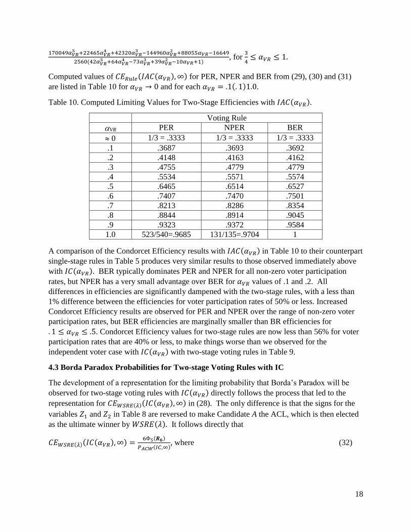
Computed values of 𝐶𝐸𝑅𝑢𝑙𝑒(𝐼𝐴𝐶(𝛼𝑉𝑅),∞) for PER, NPER and BER from (29), (30) and (31)

are listed in Table 10 for 𝛼𝑉𝑅 → 0 and for each 𝛼𝑉𝑅 = .1(. 1)1.0.

Table 10. Computed Limiting Values for Two-Stage Efficiencies with 𝐼𝐴𝐶(𝛼𝑉𝑅).

Voting Rule

VR PER NPER BER

0 1/3 = .3333 1/3 = .3333 1/3 = .3333

.1 .3687 .3693 .3692

.2 .4148 .4163 .4162

.3 .4755 .4779 .4779

.4 .5534 .5571 .5574

.5 .6465 .6514 .6527

.6 .7407 .7470 .7501

.7 .8213 .8286 .8354

.8 .8844 .8914 .9045

.9 .9323 .9372 .9584

1.0 523/540=.9685 131/135=.9704 1

A comparison of the Condorcet Efficiency results with 𝐼𝐴𝐶(𝛼𝑉𝑅) in Table 10 to their counterpart

single-stage rules in Table 5 produces very similar results to those observed immediately above

with 𝐼𝐶(𝛼𝑉𝑅). BER typically dominates PER and NPER for all non-zero voter participation

rates, but NPER has a very small advantage over BER for 𝛼𝑉𝑅 values of .1 and .2. All

differences in efficiencies are significantly dampened with the two-stage rules, with a less than

1% difference between the efficiencies for voter participation rates of 50% or less. Increased

Condorcet Efficiency results are observed for PER and NPER over the range of non-zero voter

participation rates, but BER efficiencies are marginally smaller than BR efficiencies for

. 1 ≤ 𝛼𝑉𝑅 ≤ .5. Condorcet Efficiency values for two-stage rules are now less than 56% for voter

participation rates that are 40% or less, to make things worse than we observed for the

independent voter case with 𝐼𝐶(𝛼𝑉𝑅) with two-stage voting rules in Table 9.

4.3 Borda Paradox Probabilities for Two-stage Voting Rules with IC

The development of a representation for the limiting probability that Borda’s Paradox will be

observed for two-stage voting rules with 𝐼𝐶(𝛼𝑉𝑅) directly follows the process that led to the

representation for 𝐶𝐸𝑊𝑆𝑅𝐸(𝜆)(𝐼𝐶(𝛼𝑉𝑅),∞) in (28). The only difference is that the signs for the

variables 𝑍1 and 𝑍2 in Table 8 are reversed to make Candidate A the ACL, which is then elected

as the ultimate winner by 𝑊𝑆𝑅𝐸(𝜆). It follows directly that

𝐶𝐸𝑊𝑆𝑅𝐸(𝜆)(𝐼𝐶(𝛼𝑉𝑅),∞) =6Ф5(𝑹𝟔)

𝑃𝐴𝐶𝑊(𝐼𝐶,∞), where (32)

19

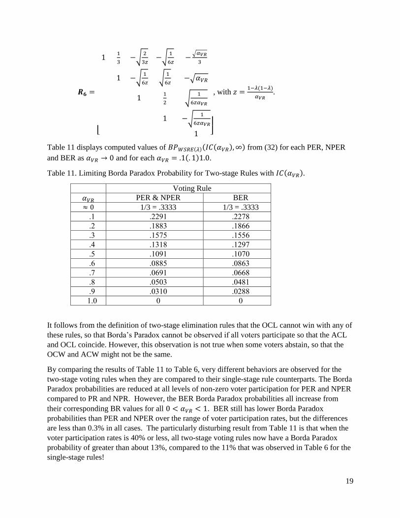
𝑹𝟔 =

[

11

3−√

2

3𝑧−√

1

6𝑧−

√𝛼𝑉𝑅

3

1 −√1

6𝑧√

1

6𝑧−√𝛼𝑉𝑅

11

2√

1

6𝑧𝛼𝑉𝑅

1 −√1

6𝑧𝛼𝑉𝑅

1 ]

, with 𝑧 =1−𝜆(1−𝜆)

𝛼𝑉𝑅.

Table 11 displays computed values of 𝐵𝑃𝑊𝑆𝑅𝐸(𝜆)(𝐼𝐶(𝛼𝑉𝑅),∞) from (32) for each PER, NPER

and BER as 𝛼𝑉𝑅 → 0 and for each 𝛼𝑉𝑅 = .1(. 1)1.0.

Table 11. Limiting Borda Paradox Probability for Two-stage Rules with 𝐼𝐶(𝛼𝑉𝑅).

Voting Rule

𝛼𝑉𝑅 PER & NPER BER

≈ 0 1/3 = .3333 1/3 = .3333

.1 .2291 .2278

.2 .1883 .1866

.3 .1575 .1556

.4 .1318 .1297

.5 .1091 .1070

.6 .0885 .0863

.7 .0691 .0668

.8 .0503 .0481

.9 .0310 .0288

1.0 0 0

It follows from the definition of two-stage elimination rules that the OCL cannot win with any of

these rules, so that Borda’s Paradox cannot be observed if all voters participate so that the ACL

and OCL coincide. However, this observation is not true when some voters abstain, so that the

OCW and ACW might not be the same.

By comparing the results of Table 11 to Table 6, very different behaviors are observed for the

two-stage voting rules when they are compared to their single-stage rule counterparts. The Borda

Paradox probabilities are reduced at all levels of non-zero voter participation for PER and NPER

compared to PR and NPR. However, the BER Borda Paradox probabilities all increase from

their corresponding BR values for all 0 < 𝛼𝑉𝑅 < 1. BER still has lower Borda Paradox

probabilities than PER and NPER over the range of voter participation rates, but the differences

are less than 0.3% in all cases. The particularly disturbing result from Table 11 is that when the

voter participation rates is 40% or less, all two-stage voting rules now have a Borda Paradox

probability of greater than about 13%, compared to the 11% that was observed in Table 6 for the

single-stage rules!

20

4.4 Borda Paradox Probabilities for Two-stage Voting Rules with IAC

Representations are also obtained for the limiting probabilities 𝐵𝑃𝑃𝐸𝑅(𝐼𝐴𝐶(𝛼𝑉𝑅),∞),

𝐵𝑃𝑁𝑃𝐸𝑅(𝐼𝐴𝐶(𝛼𝑉𝑅),∞) and 𝐵𝑃𝐵𝐸𝑅(𝐼𝐴𝐶(𝛼𝑉𝑅),∞) by using the same process that lead

respectively to the Condorcet Efficiency results in (29), (30) and (31). These resulting limiting

probability representations are given by:

𝐵𝑃𝑃𝐸𝑅(𝐼𝐴𝐶(𝛼𝑉𝑅),∞) = (33)

[30368797609𝛼𝑉𝑅

5 −147521223660𝛼𝑉𝑅4 +268423789950𝛼𝑉𝑅

3 −234843935040𝛼𝑉𝑅2

+100358455680𝛼𝑉𝑅−16930529280]

806215680(42𝛼𝑉𝑅5 −274𝛼𝑉𝑅

4 +603𝛼𝑉𝑅3 −624𝛼𝑉𝑅

2 +315𝛼𝑉𝑅−63), 0 ≤ 𝛼𝑉𝑅 ≤

1

2

[8600974249𝛼𝑉𝑅

10 −56418851820𝛼𝑉𝑅9 +150514746750𝛼𝑉𝑅

8 −197354905920𝛼𝑉𝑅7 +95067665280𝛼𝑉𝑅

6

+81478172160𝛼𝑉𝑅5 −161633646720𝛼𝑉𝑅

4 +115641561600𝛼𝑉𝑅3 −43875768960𝛼𝑉𝑅

2 +8692012800𝛼𝑉𝑅−711737280]

806215680(𝛼𝑉𝑅−1)5(42𝛼𝑉𝑅5 +64𝛼𝑉𝑅

4 −73𝛼𝑉𝑅3 +39𝛼𝑉𝑅

2 −10𝛼𝑉𝑅+1) ,

1

2≤ 𝛼𝑉𝑅 ≤

2

3

[1484308489𝛼𝑉𝑅

10 −10365275280𝛼𝑉𝑅9 +32356702665𝛼𝑉𝑅

8 −59403130380𝛼𝑉𝑅7 +70958056995𝛼𝑉𝑅

6

−57586120074𝛼𝑉𝑅5 +32164285545𝛼𝑉𝑅

4 −12237314760𝛼𝑉𝑅3 +3052242810𝛼𝑉𝑅

2 −454677300𝛼𝑉𝑅+30921993]

12597120(𝛼𝑉𝑅−1)5(42𝛼𝑉𝑅5 +64𝛼𝑉𝑅

4 −73𝛼𝑉𝑅3 +39𝛼𝑉𝑅

2 −10𝛼𝑉𝑅+1) ,

2

3≤ 𝛼𝑉𝑅 ≤

3

4

(1−𝛼𝑉𝑅)(25239𝛼𝑉𝑅4 −36326𝛼𝑉𝑅

3 +28314𝛼𝑉𝑅2 −6546𝛼𝑉𝑅−6)

1920(42𝛼𝑉𝑅5 +64𝛼𝑉𝑅

4 −73𝛼𝑉𝑅3 +39𝛼𝑉𝑅

2 −10𝛼𝑉𝑅+1) ,

3

4≤ 𝛼𝑉𝑅 ≤ 1.

𝐵𝑃𝑁𝑃𝐸𝑅(𝐼𝐴𝐶(𝛼𝑉𝑅),∞) = (34)

238551113𝛼𝑉𝑅5 −1159474830𝛼𝑉𝑅

4 +2109732075𝛼𝑉𝑅3 −1844208000𝛼𝑉𝑅

2 +786576420𝛼𝑉𝑅 −132269760

6298560(42𝛼𝑉𝑅5 −274𝛼𝑉𝑅

4 +603𝛼𝑉𝑅3 −624𝛼𝑉𝑅

2 +315𝛼𝑉𝑅−63) , 0 ≤ 𝛼𝑉𝑅 ≤

1

2

[388210400𝛼𝑉𝑅

10 −3308366400𝛼𝑉𝑅9 +14344659360𝛼𝑉𝑅

8 −39847541760𝛼𝑉𝑅7 +74031874560𝛼𝑉𝑅

6 −92271384576𝛼𝑉𝑅5

+76451921280𝛼𝑉𝑅4 −41116999680𝛼𝑉𝑅

3 +13647404880𝛼𝑉𝑅2 −2517455700𝛼𝑉𝑅+197676369

]

201553920(1−𝛼𝑉𝑅)5(42𝛼𝑉𝑅5 +64𝛼𝑉𝑅

4 −73𝛼𝑉𝑅3 +39𝛼𝑉𝑅

2 −10𝛼𝑉𝑅+1) ,

1

2≤ 𝛼𝑉𝑅 ≤

3

4

(1−𝛼𝑉𝑅 )(24471𝛼𝑉𝑅4 −66184𝛼𝑉𝑅

3 +66276𝛼𝑉𝑅2 −25284 𝛼𝑉𝑅+3171)

960(42𝛼𝑉𝑅5 +64𝛼𝑉𝑅

4 −73𝛼𝑉𝑅3 +39𝛼𝑉𝑅

2 −10𝛼𝑉𝑅+1) ,

3

4≤ 𝛼𝑉𝑅 ≤ 1.

𝐵𝑃𝐵𝐸𝑅(𝐼𝐴𝐶(𝛼𝑉𝑅),∞) = (35)

10663043𝛼𝑉𝑅5 −51663168𝛼𝑉𝑅

4 +93817521𝛼𝑉𝑅3 −81924048𝛼𝑉𝑅

2 +34935138𝛼𝑉𝑅−5878656

279936(42𝛼𝑉𝑅5 −274𝛼𝑉𝑅

4 +603𝛼𝑉𝑅3 −624𝛼𝑉𝑅

2 +315𝛼𝑉𝑅−63) , 0 ≤ 𝛼𝑉𝑅 ≤

1

2

[3104771𝛼𝑉𝑅

10 −20030400𝛼𝑉𝑅9 +52876881𝛼𝑉𝑅

8 −68907024𝛼𝑉𝑅7 +33098058𝛼𝑉𝑅

6

+28291032𝛼𝑉𝑅5 −56122794𝛼𝑉𝑅

4 +40153320𝛼𝑉𝑅3 −15234642𝛼𝑉𝑅

2 +3018060𝛼𝑉𝑅−247131]

279936(𝛼𝑉𝑅−1)5(42𝛼𝑉𝑅5 +64𝛼𝑉𝑅

4 −73𝛼𝑉𝑅3 +39𝛼𝑉𝑅

2 −10𝛼𝑉𝑅+1) ,

1

2≤ 𝛼𝑉𝑅 ≤

3

5

[794736𝛼𝑉𝑅

10 −7818275𝛼𝑉𝑅9 +33936246𝛼𝑉𝑅

8 −86024484𝛼𝑉𝑅7 +140947128𝛼𝑉𝑅

6

−155365938𝛼𝑉𝑅5 +116001396𝛼𝑉𝑅

4 −57518100𝛼𝑉𝑅3 +17990262𝛼𝑉𝑅

2 −3186459𝛼𝑉𝑅+243486]

186624(1−𝛼𝑉𝑅)5(42𝛼𝑉𝑅5 +64𝛼𝑉𝑅

4 −73𝛼𝑉𝑅3 +39𝛼𝑉𝑅

2 −10𝛼𝑉𝑅+1),

3

5≤ 𝛼𝑉𝑅 ≤

3

4

(𝛼𝑉𝑅−1)(528𝛼𝑉𝑅4 −581𝛼𝑉𝑅

3 −1524𝛼𝑉𝑅2 +855𝛼𝑉𝑅−118)

256(42𝛼𝑉𝑅5 +64𝛼𝑉𝑅

4 −73𝛼𝑉𝑅3 +39𝛼𝑉𝑅

2 −10𝛼𝑉𝑅+1), 3

4≤ 𝛼𝑉𝑅 ≤ 1.

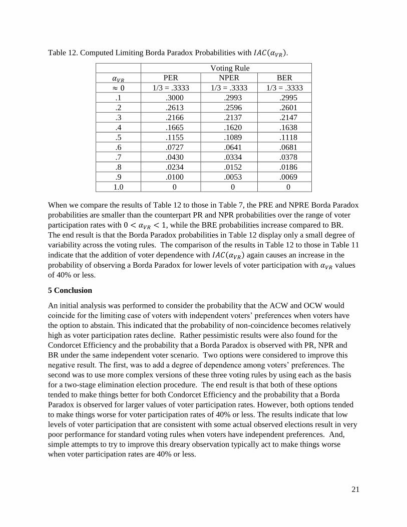
Computed values for the Borda Paradox probabilities in (33), (34) and (35) for each PER, NPER

and BER respectively are listed in Table 12 as 𝛼𝑉𝑅 → 0 and for each 𝛼𝑉𝑅 = .1(. 1)1.0.

21

Table 12. Computed Limiting Borda Paradox Probabilities with 𝐼𝐴𝐶(𝛼𝑉𝑅).

Voting Rule

𝛼𝑉𝑅 PER NPER BER

≈ 0 1/3 = .3333 1/3 = .3333 1/3 = .3333

.1 .3000 .2993 .2995

.2 .2613 .2596 .2601

.3 .2166 .2137 .2147

.4 .1665 .1620 .1638

.5 .1155 .1089 .1118

.6 .0727 .0641 .0681

.7 .0430 .0334 .0378

.8 .0234 .0152 .0186

.9 .0100 .0053 .0069

1.0 0 0 0

When we compare the results of Table 12 to those in Table 7, the PRE and NPRE Borda Paradox

probabilities are smaller than the counterpart PR and NPR probabilities over the range of voter

participation rates with 0 < 𝛼𝑉𝑅 < 1, while the BRE probabilities increase compared to BR.

The end result is that the Borda Paradox probabilities in Table 12 display only a small degree of

variability across the voting rules. The comparison of the results in Table 12 to those in Table 11

indicate that the addition of voter dependence with 𝐼𝐴𝐶(𝛼𝑉𝑅) again causes an increase in the

probability of observing a Borda Paradox for lower levels of voter participation with 𝛼𝑉𝑅 values

of 40% or less.

5 Conclusion

An initial analysis was performed to consider the probability that the ACW and OCW would

coincide for the limiting case of voters with independent voters’ preferences when voters have

the option to abstain. This indicated that the probability of non-coincidence becomes relatively

high as voter participation rates decline. Rather pessimistic results were also found for the

Condorcet Efficiency and the probability that a Borda Paradox is observed with PR, NPR and

BR under the same independent voter scenario. Two options were considered to improve this

negative result. The first, was to add a degree of dependence among voters’ preferences. The

second was to use more complex versions of these three voting rules by using each as the basis

for a two-stage elimination election procedure. The end result is that both of these options

tended to make things better for both Condorcet Efficiency and the probability that a Borda

Paradox is observed for larger values of voter participation rates. However, both options tended

to make things worse for voter participation rates of 40% or less. The results indicate that low

levels of voter participation that are consistent with some actual observed elections result in very

poor performance for standard voting rules when voters have independent preferences. And,

simple attempts to try to improve this dreary observation typically act to make things worse

when voter participation rates are 40% or less.

22

References

Cheng MC (1969) The orthant probability of four Gaussian variables. Annals of Mathematical

Statistics 40: 152-161.

Condorcet M de (1785) An essay on the application of probability theory to plurality decision

making. In Iain McLean and Fiona Hewitt (eds), Condorcet: Foundations of social choice and

political theory. Hants (England) and Brookfield (USA): Edward Elgar Press: pp 120-130.

Daunou PCF (1803) A paper on elections by ballot. In: Sommerlad F, McLean I (1991, eds) The

political theory of Condorcet II, University of Oxford Working Paper, Oxford, pp 235-279.

Fishburn PC, Gehrlein WV (1976) Borda's rule, positional voting, and Condorcet's simple majority

principle. Public Choice 28: 79-88.

Gehrlein WV (1979) A Representation for quadrivariate normal positive orthant probabilities.

Communications in Statistics, Part B 8: 349-358.

Gehrlein WV (2017) Computing multivariate normal positive orthant probabilities with 4 and 5

variables. Available at www.researchgate.net: Publication 320467212.

Gehrlein WV, Fishburn PC (1978) Probabilities of election outcomes for large electorates. Journal

of Economic Theory 19: 38-49.

Gehrlein WV, Fishburn PC (1979) Effects of abstentions on voting procedures in three-candidate

elections. Behavioral Science 24: 346-354.

Gehrlein WV, Lepelley D (2011) Voting paradoxes and group coherence: The Condorcet

efficiency of voting rules. Springer Publishing, Berlin.

Gehrlein WV, Lepelley D (2017a) Elections, voting rules and paradoxical outcomes. Springer

Publishing, Berlin.

Gehrlein WV, Lepelley D (2017b) The impact of abstentions on election outcomes when voters

have dependent preferences. Available at www.researchgate.net: Publication 316276995.

Guilbaud GT (1952) Les theories de l'intérêt general et le probleme logique de l'agregation.

Economie Appliquée 5: 501-584.

Lepelley D, Louichi A and Smaoui H (2008). On Ehrhart polynomials and probability calculations

in voting theory. Social Choice and Welfare 30: 363-383.

McDonald M (2018) United States Election Project at http://www.electproject.org/home/voter-

turnout/voter-turnout-data.

View publication statsView publication stats