the taylor rule and interest rate uncertainty in the u.s
TRANSCRIPT
Munich Personal RePEc Archive
The Taylor rule and interest rate
uncertainty in the U.S. 1955-2006
Mandler, Martin
University of Giessen
March 2007
Online at https://mpra.ub.uni-muenchen.de/2340/
MPRA Paper No. 2340, posted 22 Mar 2007 UTC
The Taylor Rule and Interest Rate Uncertainty in the
U.S. 1955-2006
Martin Mandler
(University of Giessen, Germany)
First version, March 2007
Abstract
We use a Taylor rule with time-varying policy coefficients in combination with an unobserved compo-
nents model for the output gap to estimate the uncertainty about future values of the Federal Funds
Rate. The model makes it possible to separate ex-ante interest rate uncertainty into three compo-
nents: 1) uncertainty about the Fed’s future policy coefficients, 2) uncertainty about future economic
fundamentals, and 3) residual uncertainty. The results show important changes in uncertainty about
future short-term interest rates over time with peaks in the late 1960s/early 1970s, mid 1970s and late
1970s/early 1980s. While for one-quarter forecasts uncertainty about the Fed’s policy reaction is more
important than uncertainty about economic fundamentals this result is reversed for the two-quarter
forecast horizon. Results from a modified model with regime shifts in the variance of the policy shocks
confirm the previous findings but show changes in residual uncertainty to be important as well.
Keywords: Monetary policy rules, Interest rate uncertainty, Kalman filter
JEL Classification: E52, C32, C53
Martin Mandler
University of Giessen
Department of Economics and Business
Licher Str. 62, D – 35394 Giessen
Germany
phone: +49(0)641–9922173, fax: +49(0)641–9922179
email: [email protected]–giessen.de
1 Introduction
Participants in financial markets devote considerable effort to predict how central banks
will set interest rates in the future (e.g. Meulendyke (1998)). At the same time,
an essential task of central banks’ communication policy is to “guide” expectations
about its future policy moves (e.g. ECB (2004), p. 68, Reinhart (2003)). First,
influencing expectations of future interest rates provides the central bank with some
leverage over longer-term interest rates through the term structure. Second, in their
communication central banks often try to keep uncertainty about future interest rates
low. Rising uncertainty about future moves by the central bank can have negative
effects on economic stability (e.g. Poole (2005)). For example, the resulting increase in
the volatility of money market rates can be transmitted through the yield curve (Ayuso
et al. (1997)) with the consequence of the volatility of longer-term interest rates to rise
as well, which can negatively affect economic performance.1 Because of its importance
for the efficiency of monetary policy central banks are interested in estimating interest
rate uncertainty on the market. Evidence for this is the growing research – mostly
from central bank economists – on the estimation of market expectations from financial
derivatives.2 From the financial sector’s point of view estimates of uncertainty about
future interest rates are important as well, for example for the pricing of financial
derivatives and for risk management.
The Taylor rule (Taylor (1993)) is often used as an approximate description of how cen-
tral banks set short-term interest rates in response to (expected) economic conditions.
Even though central banks certainly do not mechanically follow the Taylor rule when
deciding about monetary policy, financial market participants often use Taylor-type
rules as a tool to form expectations about how the central bank will set interest rates
in the future. Using interest rate rules to forecast policy makes it necessary to form
expectations of the economic conditions the central bank will have to react to in the
future. The uncertainty about forecasts of the information the central bank will have
1The empirical effects of interest-rate volatility on real growth in the U.S. are studied in Muell-
bauer and Nunziata (2004). Byrne and Davis (2005) investigate the effects of long-run interest rate
uncertainty on investment in the G7 economies.2For a survey of this literature, see Mandler (2003).
1
to act upon is one source of uncertainty about future interest rates (uncertainty about
future fundamentals).
However, the parameters in simple interest rate rules have been shown to change over
time. One reason for this is that a central bank does not always react in the same
way to identical economic conditions because of shifts in the weights attached to the
different goals in the central bank’s objective function. Another possible explanation is
that simple interest rate rules are only very crude approximations to optimal monetary
policy reaction functions. The information set central banks base their policy decisions
on is much richer than, for example, the (forecasts of) output gap and inflation con-
sidered in the Taylor rule. Consequently, situations with identical (forecast) values of
the output gap and inflation can be significantly different economically if judged by
the much larger optimal information set. Thus, the central bank has not necessarily
to react to (apparently) identical economic situations in the same way and this would
show up in changing policy rule parameters. A third reason for varying responses of
monetary policy can be changes in the monetary policy transmission mechanism, that
is in the structure of the economy. Variation in the coefficients of the central bank’s
reaction function causes uncertainty about how the central bank will react to given
economic conditions in the future. This is the source of a second component of interest
rate uncertainty (parameter uncertainty).
Finally, there remains a third element of interest rate uncertainty that is related to the
error term in empirically estimated Taylor rules. It represents the approximation error
of the Taylor rule relative to actual monetary policy.3
We build an empirical model of U.S. monetary policy that allows us to separate the
different components of uncertainty about future interest rates. Our model consists
of a Taylor rule with time-varying coefficients which describes how the Federal Funds
rate responds to the contemporaneously unobservable economic conditions. Changes
in the systematic reaction of monetary policy are captured by modelling the Taylor
rule parameters as driftless random walks (e.g. Cooley and Prescott (1978)). We also
3The latter two components, i.e. parameter uncertainty and residual uncertainty could be reduced
by the central bank following the approximating policy rule more strictly.
2
consider a modified version of the model that allows for heteroskedasticity in the Taylor
rule residual (Boivin (2006)). The current state of the economy is modelled using an
unobserved component model of output, inflation and the output gap as in Kuttner
(1994). This model also provides the forecasts for the output gap and inflation that
are used to predict future interest rates.
Our model adds the growing empirical literature on time-varying monetary policy rules
but provides a new field of application, namely the study of uncertainty about future
monetary policy. Previous studies have focused on ex-post descriptions of Federal Re-
serve policy: Clarida, Galì and Gertler (2000) provide evidence of pronounced changes
in Taylor-type interest rate rules for the U.S. using split-sample regression analysis.
They show a strong shift in the conduct of monetary policy related to the appointment
of Fed Chairman Volcker in 1979. More recently Boivin (2006) estimates forward-
looking Taylor rules with time-varying parameters and reports important but gradual
changes in the coefficients. Trecroci and Vassali (2006) show that time-varying mon-
etary policy reaction functions for the U.S., the U.K., Germany, France and Italy
perform superior to constant parameter rules in accounting for observed changes in
policy rates.4 Trehan and Wu (2004) estimate a time-varying parameter Taylor rule
for the U.S. focussing on changes in the equilibrium real interest rate.
An important issue in empirical estimations of monetary policy rules is that estima-
tion on ex-post data, that would not have been available to policymakers, can lead to
distorted policy coefficients (e.g. Orphanides (2001)).5 In this paper, we approach the
real-time data issue by assuming that the Fed is unable to contemporaneously observe
the relevant economic variables and thus has to rely on estimates of the state of the
economy. These estimates are derived from an unobserved components model and are
subject to revision if new information becomes available.
The empirical fact of important time-variation in uncertainty about short-term U.S.
interest rates has been documented, for example, by Fornari (2005) using implied
volatilities from swaptions. Sun (2005) finds evidence for regime shifts in the volatility
of short-term interest rates in the U.S. as well as in other countries. Empirical mod-
4Time-varying Taylor rules have also been estimated for the Deutsche Bundesbank by Kuzin (2005)
and using a regime-switching model by Assenmacher-Wesche (2006).5See also Orphanides (2002, 2003) for a discussion of the results in Clarida, Galì and Gertler (2000).
3
els of interest rate uncertainty mostly have derived their measures of uncertainty as
conditional variances from ARCH/GARCH models (e.g. Chuderewicz (2002), Lanne
and Saikkonen (2003)) or from stochastic volatility models or variants thereof (e.g.
Caporale and Cipollini (2002)). An advantage of our approach is that our measure of
interest rate uncertainty is not only derived from the time series of historical interest
rate changes but from the way financial markets perceive monetary policy to be made.
Thus, we can directly relate various components of interest rate uncertainty to their
economic sources, that is to changes in the behavior of the Fed and uncertainty about
future economic conditions.
Our approach is also partially related to the study of Favero and Mosca (2001) on
the expectations hypothesis of the term structure. They estimate monetary policy re-
action functions for the three-month rate and combine interest-rate forecasts derived
from these with a term-structure relationship. The effects of current and future short-
term interest rates on the six-month rate are allowed to depend on uncertainty about
monetary policy. They show that the expectation hypothesis cannot be rejected in
periods of low monetary policy uncertainty.
Our paper is structured as follows. Section 2 specifies the Taylor rule and the output-
inflation model and describes the estimation procedure. Section 3 presents the em-
pirical estimates for our model while section 4 contains the results for interest rate
uncertainty. Finally, section 5 concludes.
2 A model of policy and economic fundamentals
2.1 The Taylor rule
When the central bank sets the short-term interest rate in response to the current or
expected state of the economy uncertainty about future short-term interest rates stems
from (i) uncertainty about the future state of the economy and (ii) uncertainty about
the policy response to the state of the economy. The first type of uncertainty concerns
forecasts made about future values of the variables contained in the central bank’s
reaction function while the second type concerns future values of the coefficients in the
4
reaction function.
We assume that the central bank follows a Taylor-type rule in setting its policy rate.
It is not necessary that the central bank exactly follows such a rule but that financial
participants perceive the central bank to do so or use a Taylor rule to describe the
setting of the short-run interest rate
it = rt + πt + απ(πt − πt) + αzzt, (1)
where rt is the (time-varying) equilibrium real interest rate, πt is the inflation rate, π
the target value for the inflation rate, and zt is the output gap. The interest rate rule
can be rewritten as
it = α0,t + αππt + αzzt, (2)
where α0,t = rt + πt − αππt.
In empirical work it is standard practice to allow for the gradual adjustment of the
interest rate to its target level by including a lagged interest rate term, i.e.
it = (1 − ρ)(α0,t + αππt + αzzt) + ρit−1. (3)
If we allow for a time-varying response to economic conditions we can rewrite (3) as
it = β0,t + βπ,tπt + βz,tzt + ρtit−1 + ǫt, (4)
where we have also included an error term that captures the non-systematic component
of monetary policy or the approximation error of the Taylor rule relative to the actually
followed policy.
We assume that the central bank cannot observe the contemporaneous values of infla-
tion and of the output gap and therefore has to rely on estimates based on last period’s
data
5
it = β0,t + βπ,tπt|t−1 + βz,tzt|t−1 + ρtit−1 + ǫt, (5)
where xt|t−1 denotes the conditional expectation of variable x in period t based on
information available in period t − 1.
2.2 Output gap and inflation forecasts
The dynamics of the output gap and inflation rate are jointly modeled using the unob-
served components model described in Kuttner (1994). The output equation is based
on Watson (1986) and decomposes the log of real GDP (y) into a random walk and a
stationary AR(2) component
yt = nt + zt (6)
zt = φ1zt−1 + φ2zt−2 + ezt (7)
nt = μy + nt−1 + ent . (8)
n is the trend component and follows a random walk with drift μy while z is the (log)
deviation of real GDP from potential output, i.e. the output gap.
Inflation dynamics are modelled as an ARIMA process in which the change in the rate
of inflation depends on the lagged output gap
∆πt = μπ + γzt−1 + νt + δ1νt−1 + δ2νt−2 + δ3νt−3 + δ4νt−4. (9)
Writing the model (6)-(9) in state-space form we arrive at the observation equation
6
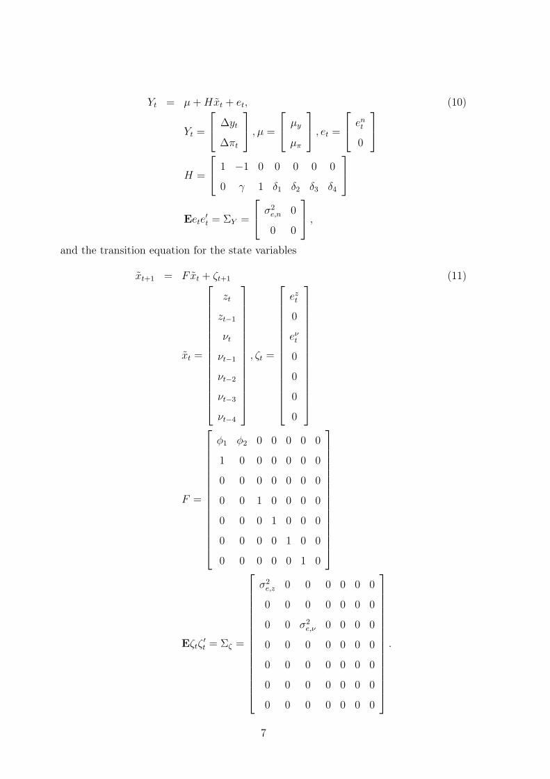
Yt = μ + Hxt + et, (10)
Yt =
⎡
⎣
∆yt
∆πt
⎤
⎦ , μ =
⎡
⎣
μy
μπ
⎤
⎦ , et =
⎡
⎣
ent
0
⎤
⎦
H =
⎡
⎣
1 −1 0 0 0 0 0
0 γ 1 δ1 δ2 δ3 δ4
⎤
⎦
Eete′t = ΣY =
⎡
⎣
σ2e,n 0
0 0
⎤
⎦ ,
and the transition equation for the state variables
xt+1 = Fxt + ζt+1 (11)
xt =
⎡
⎢
⎢
⎢
⎢
⎢
⎢
⎢
⎢
⎢
⎢
⎢
⎢
⎢
⎢
⎢
⎣
zt
zt−1
νt
νt−1
νt−2
νt−3
νt−4
⎤
⎥
⎥
⎥
⎥
⎥
⎥
⎥
⎥
⎥
⎥
⎥
⎥
⎥
⎥
⎥
⎦
, ζt =
⎡
⎢
⎢
⎢
⎢
⎢
⎢
⎢
⎢
⎢
⎢
⎢
⎢
⎢
⎢
⎢
⎣
ezt
0
eνt
0
0
0
0
⎤
⎥
⎥
⎥
⎥
⎥
⎥
⎥
⎥
⎥
⎥
⎥
⎥
⎥
⎥
⎥
⎦
F =
⎡
⎢
⎢
⎢
⎢
⎢
⎢
⎢
⎢
⎢
⎢
⎢
⎢
⎢
⎢
⎢
⎣
φ1 φ2 0 0 0 0 0
1 0 0 0 0 0 0
0 0 0 0 0 0 0
0 0 1 0 0 0 0
0 0 0 1 0 0 0
0 0 0 0 1 0 0
0 0 0 0 0 1 0
⎤
⎥
⎥
⎥
⎥
⎥
⎥
⎥
⎥
⎥
⎥
⎥
⎥
⎥
⎥
⎥
⎦
Eζtζ′t = Σζ =
⎡
⎢
⎢
⎢
⎢
⎢
⎢
⎢
⎢
⎢
⎢
⎢
⎢
⎢
⎢
⎢
⎣
σ2e,z 0 0 0 0 0 0
0 0 0 0 0 0 0
0 0 σ2e,ν 0 0 0 0
0 0 0 0 0 0 0
0 0 0 0 0 0 0
0 0 0 0 0 0 0
0 0 0 0 0 0 0
⎤
⎥
⎥
⎥
⎥
⎥
⎥
⎥
⎥
⎥
⎥
⎥
⎥
⎥
⎥
⎥
⎦
.
7

We assume that the shocks eν , en and ez are serially and mutually uncorrelated.
This model can be estimated by maximum likelihood using the Kalman filter. From
the Kalman filter we obtain estimates of the current value of the output gap based
on information from the previous period as zt|t−1 which is the first element of xt|t−1,
the forecast of the state vector based on information from the last period. We use
this estimate, together with the inflation forecast πt|t−1 = πt−1 + ∆πt|t−1 as exogenous
variables in the estimation of the Taylor rule (5). Thus we assume that either the
central bank uses this or a related model to estimate the current state of the economy
or that financial market participants accept this model as an approximation of how the
central bank arrives at its estimates of economic fundamentals. Therefore, we later use
this model to make forecasts of future output gaps and inflation to be used as inputs
for the interest rate forecasts.
The interest rate rule model can be written in state-space form as
it = x′tβt + ǫt, (12)
x′t =
[
1 πt|t−1 zt|t−1 it−1
]
Eǫ2
t = σ2
ǫ . (13)
The time-varying parameters follow a random walk
βt+1 = βt + wt+1 (14)
βt =
⎡
⎢
⎢
⎢
⎢
⎢
⎢
⎣
β0,t
βπ,t
βz,t
ρt
⎤
⎥
⎥
⎥
⎥
⎥
⎥
⎦
, wt =
⎡
⎢
⎢
⎢
⎢
⎢
⎢
⎣
wct
wπt
wzt
wit
⎤
⎥
⎥
⎥
⎥
⎥
⎥
⎦
Ewtw′t = Σw.
The shocks w and ǫ are serially and mutually uncorrelated, as well as uncorrelated
with any shocks in the output gap/inflation model. However, we allow for correlation
among the shocks in w.6 The parameters of this model can again be estimated by
6This is a consequence of the standardization implicit in the estimation approach that will be used.
8
maximum likelihood and application of the Kalman filter. Later we will interpret the
estimates of the time-varying parameters β as representing market participants’ view
of the currently relevant central bank reaction function and use the estimated policy
rule for forecasting future interest rates.
2.3 Estimation
Using the estimates from the output gap/inflation model to estimate the interest rate
rule parameters requires two basic assumptions. First, we assume that the contempo-
raneous value of xt that underlies the central bank’s decision is known to the public.
That is, we assume that the central bank publishes or announces its estimates of the
contemporaneous inflation rate and the output gap that enter the interest rate deci-
sion. Second, xt must be exogenous to βt. For example, our model does not allow
for asymmetries in the interest rate response to the output gap or inflation, i.e. for
the β parameters to vary systematically with changes in the estimated output gap or
inflation rate.
Since the parameters of the interest rate rule follow a random walk we have to deal with
the “pile-up” problem as discussed in Stock (1994). Basically, if the variances in Σw are
small their maximum likelihood estimates will be biased toward zero. Following Stock
and Watson’s (1998) median unbiased estimation procedure we rewrite the observation
equation as
∆βt = wt = τηt, τ = λ/T (15)
with η being a vector of mutually uncorrelated shocks that are also assumed to be un-
correlated with the policy shock ǫ. T is the number of observations.7 τ can be inferred
from performing a conventional Quandt (1960) likelihood ratio test for stability: From
the resulting test statistic QLRT we can retrieve an estimate of λ by using Table 3 in
Stock and Watson (1998), p. 354. In order to use this table we have to impose the
normalization8
7This procedure for the estimation of the variances is also applied in Boivin (1996).8See Stock and Watson (1998), p. 351.
9
Ση =σ2
ǫ
Extx′t
, (16)
where, for estimation, we replace Extx′t by 1
T
∑T
i=1xix
′i. Thus, the overall estimation
procedure for the model (10)-(14) is as follows:
1. Perform the QLRT test and obtain the estimate for λ.
2. Impose the restriction
Σw =
(
λ
T
)2σ2
ǫ
1
T
∑T
i=1xix′
i
(17)
3. Run the Kalman filter to estimate the remaining free parameter σǫ by maximum
likelihood.
3 Estimation results
The output gap/inflation model is estimated on U.S. quarterly data from 1955Q1 to
2006Q2. All data were obtained from FRED II, the database of the Federal Reserve
Bank of St. Louis. The inflation rate is defined as 100 times the annual difference of
the log Consumer Price Index. Table 1 shows the coefficient estimates. γ is positive
and significant. Thus, if output exceeds its potential (z > 0) inflation accelerates. The
point estimate implies that an output gap of 1%, i.e. output exceeding its potential by
1%, leads to an increase in the annual rate of inflation by 0.13%.9
Figure 1 shows the estimated time series of potential output (actual output minus the
estimated output gap) and the log of real GDP. As in Kuttner (1994) potential output
exhibits substantial short-run fluctuations.
« insert Figure 1 »
The deviations of actual output from its potential, i.e. the output gap, are displayed
in Figure 2 along with 1.69 standard error bounds which correspond to 90% confidence
intervals. These error bounds are constructed using the Monte Carlo approach from
9We also estimated a specification which allows for a direct effect of output growth on the change
in the inflation rate. In contrast to Kuttner (1994) the relevant coefficient always turned out to be
insignificant.
10
output equation inflation equation output gap equation
μy 0.82 (0.04) μπ 0.01 (0.08) φ1 1.46 (0.03)
γ 0.13 (0.04) φ2 -0.53 (0.06)
δ1 -.04 (0.04)
δ2 0.69 (0.06)
δ3 0.01 (0.01)
δ4 -0.11 (0.02)
σe,n 0.60 (0.07) σe,ν 0.59 ( 0.03) σe,z 0.55 (0.08)
SE 0.87 SE 0.61
Standard errors in parentheses. Estimation from 206 quarterly obser-
vations from 1955:1 to 2006:2. Log-likelihood value is:-257.29.
Table 1: Parameter estimates for the output gap - inflation model
Hamilton (1994) and reflect both the Kalman filter uncertainty and the uncertainty
about the parameter estimates.
« insert Figure 2 »
The next variable that enters the interest rate rule is the inflation forecast πt|t−1 which
is shown in Figure 3 together with the actual inflation rates.
« insert Figure 3 »
Using the time series for zt|t−1 and the inflation forecasts πt|t−1 we estimate the pa-
rameters of the time-varying Taylor rule as described in section 2. Since the standard
deviations for the time-varying response parameters were obtained using the approach
by Stock and Watson (1998), we cannot provide standard deviations for the estimates.
The fit of the time-varying Taylor rule is displayed in Figure 4. The estimated model
provides a reasonable approximation to the actually observed interest rates with a sum
of squared residuals of 197.93. As is to be expected from the random walk specification
for the response parameters the fitted interest rate lags the observed one by one period.
« insert Figure 4 »
Figure 5 shows the one-sided estimates of the time varying long-run coefficients of the
11
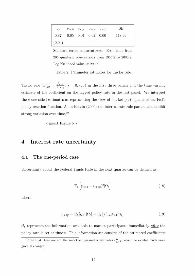
σǫ σw,0 σw,π σw,z σw,i SE
0.87 0.05 0.01 0.02 0.00 118.99
(0.04)
Standard errors in parentheses. Estimation from
205 quarterly observations from 1955:2 to 2006:2.
Log-likelihood value is:-290.51.
Table 2: Parameter estimates for Taylor rule
Taylor rule (βlrj,t|t =
βj,t|t
1−ρt|t, j = 0, π, z) in the first three panels and the time varying
estimate of the coefficient on the lagged policy rate in the last panel. We interpret
these one-sided estimates as representing the view of market participants of the Fed’s
policy reaction function. As in Boivin (2006) the interest rate rule parameters exhibit
strong variation over time.10
« insert Figure 5 »
4 Interest rate uncertainty
4.1 The one-period case
Uncertainty about the Federal Funds Rate in the next quarter can be defined as
Et
[
(it+1 − it+1|t)2|Ωt
]
, (18)
where
it+1|t = Et [it+1|Ωt] = Et
[
x′t+1βt+1|Ωt
]
. (19)
Ωt represents the information available to market participants immediately after the
policy rate is set at time t. This information set consists of the estimated coefficients
10Note that these are not the smoothed parameter estimates βlrj,t|T , which do exhibit much more
gradual changes.
12
in Tables 1 and 2 – that is we assume that the public knows the model the central
bank uses to estimate the output gap and the current inflation rate – and all past
values of y and π but not the current values of output and inflation yt and πt which
cannot be observed contemporaneously. It also contains past and current values of i
and the current values of the central bank’s estimates of the output gap zt|t−1 and of
the inflation rate πt|t−1.11
We assume β and x to be uncorrelated.12 Thus,
it+1|t = Et
[
x′t+1|Ωt
]
Et [βt+1|Ωt] = x′t+1|tβt+1|t. (20)
Note that since xt = (1 πt|t−1 zt|t−1 it−1), the forecast of xt+1 based on Ωt, is
xt+1|t = (1 πt+1|t−1 zt+1|t−1 it). However the forecast of βt+1 based on Ωt is βt+1|t
as it is part of the information set.
« insert Figure 6 »
Hence, we have
Et
[
(it+1 − it+1|t)2|Ωt
]
= Et
[
(x′t+1βt+1 − x′
t+1|tβt+1|t)2|Ωt
]
(21)
= Et
[
β′t+1xt+1x
′t+1βt+1|Ωt
]
− β′t+1|txt+1|tx
′t+1|tβt+1|t + σ2
ǫ .
This can be written as
Et
[
(it+1 − it+1|t)2|Ωt
]
= x′t+1|tEt
[
(βt+1 − βt+1|t)(βt+1 − βt+1|t)′|Ωt
]
xt+1|t
+β′t+1|tEt
[
(xt+1 − xt+1|t)(xt+1 − xt+1|t)′|Ωt
]
βt+1|t (22)
= x′t+1|tPβ,t+1|tx
′t+1|t + β′
t+1|tPx,t+1|tβt+1|t + σ2
ǫ .
Pβ,t+1|t = Et
[
(βt+1 − βt+1|t)(βt+1 − βt+1|t)′]
is obtained from the Kalman filter. This
component of the overall interest rate forecast uncertainty represents uncertainty due
11An alternative assumption would be that market participants accept the model as a relatively
accurate representation of the way the central bank acquires and uses its information.12This assumption is implied by using the Kalman filter to estimate β.
13
to changes in the way the Fed reacts to the fundamental variables in its reaction
function. The uncertainty due to this component of future interest rates rises if there
is a numerical increase in the variables that enter the policy rule. The reason is that
even when uncertainty about the β-parameters remains unchanged, uncertainty about
the size of the interest rate response of the central bank increases when the absolute
values of the variables the β-coefficients are multiplied with go up.
Px,t+1|t = Et
[
(xt+1 − xt+1|t)(xt+1 − xt+1|t)′|Ωt
]
represents the uncertainty about the
forecast of the economic variables the interest rate responds to. A detailed derivation
of this expression can be found in the Appendix.
The results are presented in Figure 7. The Figure shows the overall interest rate
uncertainty (22) together with two of its components13
βunc = x′t+1|tPβ,t+1|tx
′t+1|t
and
xunc = β′t+1|tPx,t+1|tβ
′t+1|t.
« insert Figure 7 »
The Figure shows that most of the interest rate uncertainty is caused by the variance
of the policy shock σ2ǫ . There are three episodes in which an increase in the uncertainty
about the policy response (βunc) leads to a burst in overall interest rate uncertainty.
These episodes occurred at the end of the 1960s, in the mid 1970s and in the early
1980s. The latter two episodes coincide with an increase in the forecast uncertainty
of the output gap and inflation. After the mid-1980s and particularly during the
1990s uncertainty about the policy parameters remains relatively low and rises again
somewhat after 2001. Uncertainty about future values of output gap almost always
plays a minor role relative to the interest rate rule parameter uncertainty. Uncertainty
about economic fundamentals rises over the 1970s and drops again in the early 1980s
13The high initial values result from the Kalman filter initialization where we have chosen a relatively
high starting variance for the β vector in order to discount possible effects from the choice of the
starting values.
14
to a level comparably to that of the 1960s. In the early 1990s it rises somewhat but
remains far below the levels of the 1970s.
4.2 The two-period case
We can define uncertainty about the interest rate set two periods in the future as
Et
[
(it+2 − it+2|t)2|Ωt
]
, (23)
where
it+2|t = Et [(it+2|Ωt] = Et
[
x′t+2βt+2|Ωt
]
(24)
= Et
[
x′t+2|Ωt
]
Et [βt+2|Ωt] = x′t+2|tβt+2|t.
« insert Figure 8 »
We get
Et
[
(it+2 − it+2|t)2|Ωt
]
= Et
[
(x′t+2βt+2 − x′
t+2|tβt+2|t)2|Ωt
]
(25)
= Et
[
β′t+2xt+2x
′t+2βt+2|Ωt
]
− β′t+2|txt+2|tx
′t+2|tβt+2|t + σ2
ǫ ,
and, finally,
Et
[
(it+2 − it+2|t)2|Ωt
]
= x′t+2|tEt
[
(βt+2 − βt+2|t)(βt+2 − βt+2|t)′|Ωt
]
xt+2|t
+β′t+2|tEt
[
(xt+2 − xt+2|t)(xt+2 − xt+2|t)′|Ωt
]
βt+2|t (26)
= x′t+2|tPβ,t+2|tx
′t+2|t + β′
t+2|tPx,t+2|tβ′t+2|t + σ2
ǫ .
Pβ,t+2|t = Et
[
(βt+2 − βt+2|t)(βt+2 − βt+2|t)′|Ωt
]
can be computed by noting (A4) as
Pβ,t+2|t = Pβ,t+1|t + Σw. For the derivation of Px,t+2|t refer to the appendix.
Figure 9 shows the two-period forecast uncertainty about the federal funds rate along
with its two components. It is obvious that interest rate uncertainty is markedly higher
15
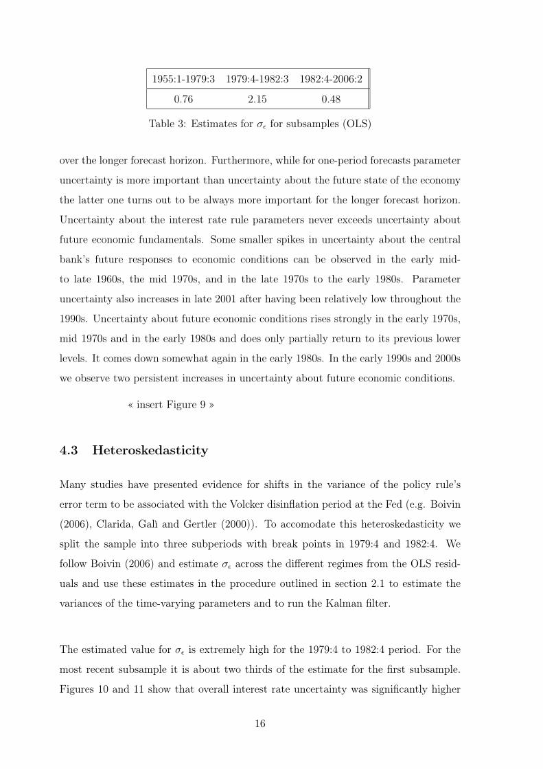
1955:1-1979:3 1979:4-1982:3 1982:4-2006:2
0.76 2.15 0.48
Table 3: Estimates for σǫ for subsamples (OLS)
over the longer forecast horizon. Furthermore, while for one-period forecasts parameter
uncertainty is more important than uncertainty about the future state of the economy
the latter one turns out to be always more important for the longer forecast horizon.
Uncertainty about the interest rate rule parameters never exceeds uncertainty about
future economic fundamentals. Some smaller spikes in uncertainty about the central
bank’s future responses to economic conditions can be observed in the early mid-
to late 1960s, the mid 1970s, and in the late 1970s to the early 1980s. Parameter
uncertainty also increases in late 2001 after having been relatively low throughout the
1990s. Uncertainty about future economic conditions rises strongly in the early 1970s,
mid 1970s and in the early 1980s and does only partially return to its previous lower
levels. It comes down somewhat again in the early 1980s. In the early 1990s and 2000s
we observe two persistent increases in uncertainty about future economic conditions.
« insert Figure 9 »
4.3 Heteroskedasticity
Many studies have presented evidence for shifts in the variance of the policy rule’s
error term to be associated with the Volcker disinflation period at the Fed (e.g. Boivin
(2006), Clarida, Galì and Gertler (2000)). To accomodate this heteroskedasticity we
split the sample into three subperiods with break points in 1979:4 and 1982:4. We
follow Boivin (2006) and estimate σǫ across the different regimes from the OLS resid-
uals and use these estimates in the procedure outlined in section 2.1 to estimate the
variances of the time-varying parameters and to run the Kalman filter.
The estimated value for σǫ is extremely high for the 1979:4 to 1982:4 period. For the
most recent subsample it is about two thirds of the estimate for the first subsample.
Figures 10 and 11 show that overall interest rate uncertainty was significantly higher
16
in the pre 1979:4-period than in the post 1982:4-period. For the 1979:4 to 1982:4
subperiod most of the drastic increase in uncertainty is due to the increased variance
of the error term ǫ, but uncertainty about the interest rate rule parameters increased
substantially as well. Uncertainty about the Taylor rule parameters is on average
higher from 1960-79 than from 1982 on. As in the homoskedastic case, there are two
spikes in parameter uncertainty at the end of 1960s and in the mid 1970s. In the
final subsample uncertainty about the Fed’s response parameters is very low and below
uncertainty about next quarter’s fundamentals. The latter one starts out very low and
slowly edges upward throughout the 1970s. We observe a strong rise in uncertainty
about future economic conditions in the mid 1980s when it makes up most of overall
interest rate uncertainty. After the mid 1980s uncertainty about future fundamentals
is relatively low again. However, on average this component of overall interest rate
uncertainty is higher after the late 1980s than in the 1960s and early 1970s.
« insert Figures 10+11 »
Figures 12 and 13 show the results for the two-period interest rate forecasts. The
overall impression is similar to the one-period case but on a higher level. As in the ho-
moskedastic case, uncertainty about the future state of the economy is more important
than uncertainty about the policy parameters.
« insert Figures 12+13 »
5 Conclusion
We have constructed an empirical model of monetary policy in the U.S. that enables
us to separate the uncertainty perceived by market participants about future interest
rates into its basic components: uncertainty about the state of the economy in the
future and uncertainty about how the Fed will react to future economic conditions.
Our results show that there is considerable time variation in the parameters of the pol-
icy rule. For forecast horizons up to one quarter uncertainty about the future values of
these parameters is most of the time more important than uncertainty about the future
state of the economy. For a forecast horizon of two quarters uncertainty about future
17
economic conditions dominates uncertainty about future policy parameters. According
to our model uncertainty about future interest rates is highly variable with peaks in the
late 1960s/early 1970s, mid 1970s and late 1970s/early 1980s. Recently, uncertainty
about future policy reactions has increased again and over the longer forecast horizon
uncertainty about future economic conditions has also gone up.
We also accounted for shifts in the error variance of the interest rate rule. We found a
strong increase in interest rate uncertainty in the 1979-1982 period, driven by a surge
in the error variance of the policy rule. The estimates from the modified model show
uncertainty about future interest rates to have been exceptionally low in the post 1990
period.
18
Appendix A: The Kalman filter equations
The estimates of the unobserved component xt|t−1 = Et−1[xt] and its covariance matrix
Px,t|t−1 = Et−1[(xt − xt|t−1)(xt − xt|t−1)′] are formed recursively
xt|t−1 = Fxt−1|t−1, (A1)
Px,t|t−1 = FPx,t−1|t−1F′ + Σζ , (A2)
with xt|t = Et[xt] and its covariance matrix Px,t|t = Et[(xt − xt|t)(xt − xt|t)′].
After the information on Yt has become available, the estimates are updated as
xt|t = xt|t−1 + Kt|t−1(Yt − Yt|t−1)
= xt|t−1 + Kt|t−1(Yt − μ − Hxt|t−1)
= xt|t−1 + Kt|t−1(H(xt − xt|t−1) + et) (A3)
Px,t|t = Px,t|t−1 − Kt|t−1HPx,t|t−1, (A4)
with Kt|t−1 = Px,t|t−1H′[HPx,t|t−1H
′ + ΣY ]−1.
The second second row of (A3) is used to form the estimate of xt|t while the third row
is used in the computation of the expressions for interest rate uncertainty.
The forecasting and updating equations for the Taylor rule coefficients are
βt|t−1 = βt−1|t−1, (A5)
Pβ,t|t−1 = Pβ,t−1|t−1 + Σw, (A6)
After the information on it has become available, the estimates are updated as
19
βt|t = βt|t−1 + Pβ,t|t−1xt[x′tPβ,t|t−1xt + σ2
ǫ ]−1(it − it|t−1)
= βt|t−1 + Pβ,t|t−1xt[x′tPβ,t|t−1xt + σ2
ǫ ]−1(it − x′
tβt|t−1), (A7)
Pβ,t|t = Pβ,t|t−1 − Pβ,t|t−1xt[x′tPβ,t|t−1xt + σ2
ǫ ]−1x′
tPβ,t|t−1. (A8)
Since we require only the one-sided estimates for x and β we do not reproduce the
equations for the smoothing algorithm.14
Appendix B: Uncertainty measures
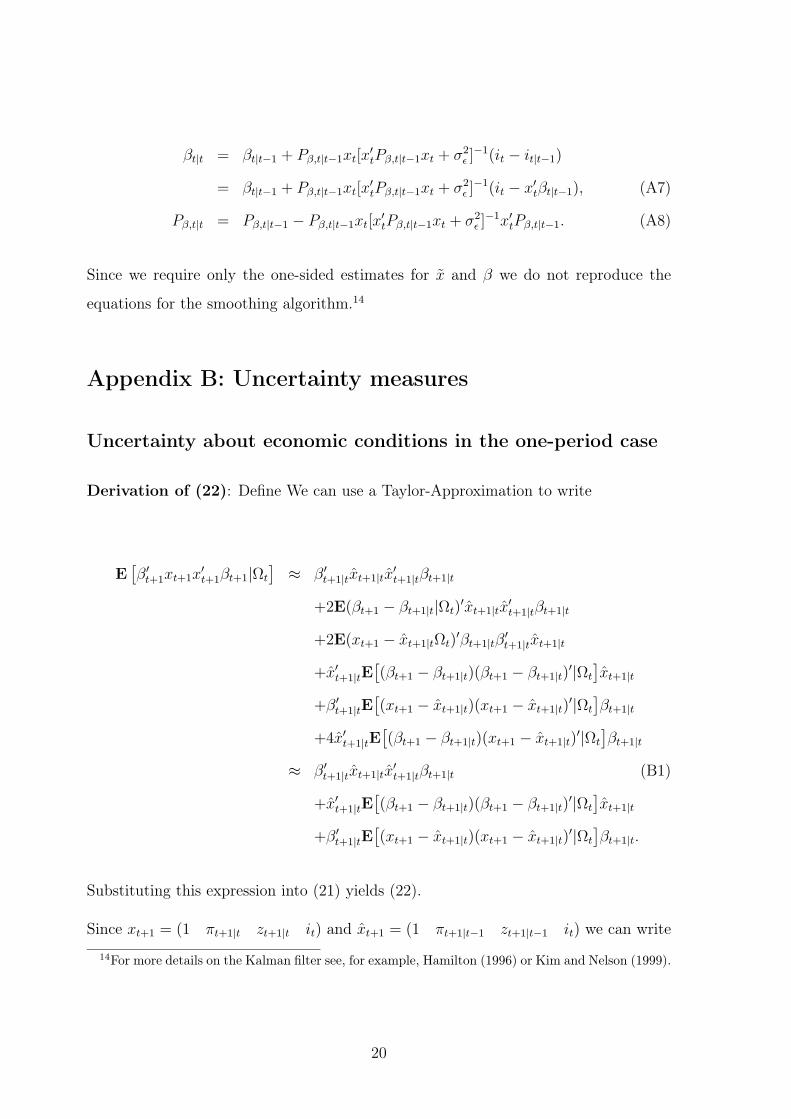
Uncertainty about economic conditions in the one-period case
Derivation of (22): Define We can use a Taylor-Approximation to write
E[
β′t+1xt+1x
′t+1βt+1|Ωt
]
≈ β′t+1|txt+1|tx
′t+1|tβt+1|t
+2E(βt+1 − βt+1|t|Ωt)′xt+1|tx
′t+1|tβt+1|t
+2E(xt+1 − xt+1|tΩt)′βt+1|tβ
′t+1|txt+1|t
+x′t+1|tE
[
(βt+1 − βt+1|t)(βt+1 − βt+1|t)′|Ωt
]
xt+1|t
+β′t+1|tE
[
(xt+1 − xt+1|t)(xt+1 − xt+1|t)′|Ωt
]
βt+1|t
+4x′t+1|tE
[
(βt+1 − βt+1|t)(xt+1 − xt+1|t)′|Ωt
]
βt+1|t
≈ β′t+1|txt+1|tx
′t+1|tβt+1|t (B1)
+x′t+1|tE
[
(βt+1 − βt+1|t)(βt+1 − βt+1|t)′|Ωt
]
xt+1|t
+β′t+1|tE
[
(xt+1 − xt+1|t)(xt+1 − xt+1|t)′|Ωt
]
βt+1|t.
Substituting this expression into (21) yields (22).
Since xt+1 = (1 πt+1|t zt+1|t it) and xt+1 = (1 πt+1|t−1 zt+1|t−1 it) we can write
14For more details on the Kalman filter see, for example, Hamilton (1996) or Kim and Nelson (1999).
20
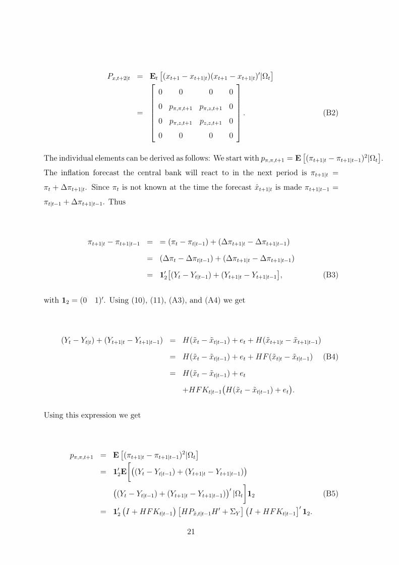
Px,t+2|t = Et
[
(xt+1 − xt+1|t)(xt+1 − xt+1|t)′|Ωt
]
=
⎡
⎢
⎢
⎢
⎢
⎢
⎢
⎣
0 0 0 0
0 pπ,π,t+1 pπ,z,t+1 0
0 pπ,z,t+1 pz,z,t+1 0
0 0 0 0
⎤
⎥
⎥
⎥
⎥
⎥
⎥
⎦
. (B2)
The individual elements can be derived as follows: We start with pπ,π,t+1 = E[
(πt+1|t − πt+1|t−1)2|Ωt
]
.
The inflation forecast the central bank will react to in the next period is πt+1|t =
πt + ∆πt+1|t. Since πt is not known at the time the forecast xt+1|t is made πt+1|t−1 =
πt|t−1 + ∆πt+1|t−1. Thus
πt+1|t − πt+1|t−1 = = (πt − πt|t−1) + (∆πt+1|t − ∆πt+1|t−1)
= (∆πt − ∆πt|t−1) + (∆πt+1|t − ∆πt+1|t−1)
= 1′2
[
(Yt − Yt|t−1) + (Yt+1|t − Yt+1|t−1
]
, (B3)
with 12 = (0 1)′. Using (10), (11), (A3), and (A4) we get
(Yt − Yt|t) + (Yt+1|t − Yt+1|t−1) = H(xt − xt|t−1) + et + H(xt+1|t − xt+1|t−1)
= H(xt − xt|t−1) + et + HF (xt|t − xt|t−1) (B4)
= H(xt − xt|t−1) + et
+HFKt|t−1
(
H(xt − xt|t−1) + et
)
.
Using this expression we get
pπ,π,t+1 = E[
(πt+1|t − πt+1|t−1)2|Ωt
]
= 1′2E
[
(
(Yt − Yt|t−1) + (Yt+1|t − Yt+1|t−1))
(
(Yt − Yt|t−1) + (Yt+1|t − Yt+1|t−1))′|Ωt
]
12 (B5)
= 1′2
(
I + HFKt|t−1
) [
HPx,t|t−1H′ + ΣY
] (
I + HFKt|t−1
]′12.
21
At the time the policy rate in period t is announced, uncertainty about πt+1|t, the
estimate of inflation the Fed will react to in the next period and which is forecast as
πt+1|t−1, stems from two sources: first, (∆πt − ∆πt|t−1), the second element of (Yt −
Yt|t−1), is the error made in estimating the change in the inflation rate from the previous
to the current period. Second, (∆πt+1|t − ∆πt+1|t−1), the (2,1) element of (Yt+1|t −
Yt+1|t−1), is the difference between the change in inflation over the next period estimated
by the central bank at the time it has to set it+1 – and thus formed with knowledge of
πt – and the estimate of next period’s change in inflation that is formed by the public
now without knowing πt.
Next we compute pz,z,t+1 = E[
(zt+1|t − zt+1|t−1)2|Ωt
]
. Since zt is the (1,1) element of
xt,
zt+1|t − zt+1|t−1 = 1′1(xt+1|t − xt+1|t−1)
= 1′1F (xt|t − xt|t−1) (B6)
= 1′1FKt|t−1
(
H(xt − xt|t−1) + et
)
.
Thus, we arrive at
pz,z,t+1 = E[
(zt+1|t − zt+1|t−1)2|Ωt
]
= 1′1E
[
(xt+1|t − xt+1|t−1)(xt+1|t − xt+1|t−1)′|Ωt
]
11 (B7)
= 1′1FKt|t−1HPx,t|t−1F
′11,
with 11 = (1 0 0 0 0 0 0)′. Uncertainty about the Fed’s estimate of the output
gap is due to the fact that when policy is set next period additional information in
form of observations of πt and yt will be available.
Finally, combining (B3) and (B4) with (B6) we get
pπ,z,t+1 = E[
(πt+1|t − πt+1|t−1)(zt+1|t − zt+1|t−1)|Ωt
]
(B8)
= 1′2
(
HPx,t|t−1F′ + HFKt|t−1HPx,t|t−1F
′)
11.
22
All these expressions can be evaluated using the parameter estimates from section 3
and the results from the Kalman filter.
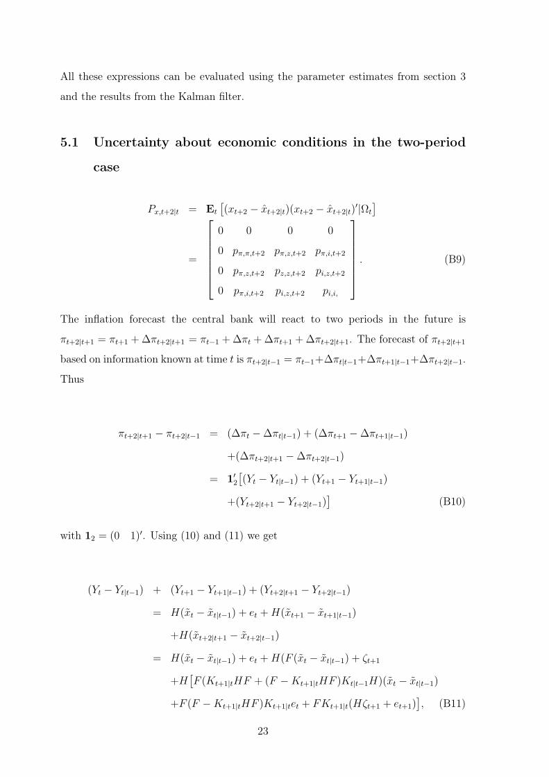
5.1 Uncertainty about economic conditions in the two-period
case
Px,t+2|t = Et
[
(xt+2 − xt+2|t)(xt+2 − xt+2|t)′|Ωt
]
=
⎡
⎢
⎢
⎢
⎢
⎢
⎢
⎣
0 0 0 0
0 pπ,π,t+2 pπ,z,t+2 pπ,i,t+2
0 pπ,z,t+2 pz,z,t+2 pi,z,t+2
0 pπ,i,t+2 pi,z,t+2 pi,i,
⎤
⎥
⎥
⎥
⎥
⎥
⎥
⎦
. (B9)
The inflation forecast the central bank will react to two periods in the future is
πt+2|t+1 = πt+1 + ∆πt+2|t+1 = πt−1 + ∆πt + ∆πt+1 + ∆πt+2|t+1. The forecast of πt+2|t+1
based on information known at time t is πt+2|t−1 = πt−1+∆πt|t−1+∆πt+1|t−1+∆πt+2|t−1.
Thus
πt+2|t+1 − πt+2|t−1 = (∆πt − ∆πt|t−1) + (∆πt+1 − ∆πt+1|t−1)
+(∆πt+2|t+1 − ∆πt+2|t−1)
= 1′2
[
(Yt − Yt|t−1) + (Yt+1 − Yt+1|t−1)
+(Yt+2|t+1 − Yt+2|t−1)]
(B10)
with 12 = (0 1)′. Using (10) and (11) we get
(Yt − Yt|t−1) + (Yt+1 − Yt+1|t−1) + (Yt+2|t+1 − Yt+2|t−1)
= H(xt − xt|t−1) + et + H(xt+1 − xt+1|t−1)
+H(xt+2|t+1 − xt+2|t−1)
= H(xt − xt|t−1) + et + H(F (xt − xt|t−1) + ζt+1
+H[
F (Kt+1|tHF + (F − Kt+1|tHF )Kt|t−1H)(xt − xt|t−1)
+F (F − Kt+1|tHF )Kt+1|tet + FKt+1|t(Hζt+1 + et+1)]
, (B11)
23
whre the expression in the last two lines of (B11) is derived in (B13). As a result we
arrive at
pπ,π,t+2 = E[
(πt+2|t+1 − πt+2|t−1)2|Ωt
]
= 1′2E
[
(
(Yt − Yt|t−1) + (Yt+1 − Yt+1|t−1) + (Yt+2|t+1 − Yt+2|t−1))
(
(Yt − Yt|t−1) + (Yt+1 − Yt+1|t−1) + (Yt+2|t+1 − Yt+2|t−1))′|Ωt
]′
12
= 1′2
[
H[
I + F(
I + Kt+1|tHF + (F − Kt+1|tHF )Kt|t−1H)]
Px,t|t−1
[
I + F(
I + Kt+1|tHF + (F − Kt+1|tHF )Kt|t−1H)]′
H ′
+HF (I + Kt+1|tH)Σζ(I + Kt+1|tH)′F ′H ′ (B12)
HF (F − Kt+1|tHF )Kt|t−1ΣY K ′t|t−1(F − Kt+1|tHF )′F ′H ′
+HFKt+1|tΣY K ′t+1|tF
′H ′
]
12.
For the squared forecasting error of the output gap estimate we have
zt+2|t+1 − zt+2|t−1 = 1′1(xt+2|t+1 − xt+2|t−1)
= 1′1F (xt+1|t + Kt+1|t[H(xt+1 − xt+1|t) + et+1] − xt|t−1)
= 1′1F
[
F (xt|t − xt|t−1) + Kt+1|t(H(F (xt − xt|t) + ζt+1) + et+1)]
= 1′1F
(
FKt|t−1[H(xt − xt|t−1) + et] + Kt+1|tHF (xt − (xt|t−1
+Kt|t−1(H(xt − xt|t−1) + et)) + Kt+1|t(Hζt+1 + et+1))
= 1′1
(
F (Kt+1|tHF + (F − Kt+1|tHF )Kt|t−1H)(xt − xt|t−1) + et)
+F (F − Kt+1|tHF )Kt|t−1et + FKt+1|t(Hζt+1 + et+1))
. (B13)
Thus,
24
pz,z,t+2 = E[
(zt+2|t+1 − zt+2|t−1)2|Ωt
]
= 1′1E
[
(xt+2|t − xt+2|t−1)(xt+2|t − xt+2|t−1)′|Ωt
]
11
= 1′1
[
F(
Kt+1|tHF + (F − Kt+1|tHF )Kt|t−1H)
Px,t|t−1
(
Kt+1|tHF + (F − Kt+1|tHF )Kt|t−1H)′
F ′ (B14)
+F[
(F − Kt+1|tHF )Kt|t−1 + Kt+1|t
]
ΣY
[
(F − Kt+1|tHF )Kt|t−1 + Kt+1|t
]′F ′
+FKt+1|tHΣζH′K ′
t+1|tF′
]
11.
From (B10), (B11) and (B13) we derive
pπ,z,t+2 = E[
(πt+2|t+1 − πt+2|t−1)(zt+2|t+1 − zt+2|t−1)|Ωt
]
= 1′2
[
H(
I + F (I + Kt+1|tHF + (F − Kt+1|tHF )Kt|t−1H)
Px,t|t−1
(
Kt+1|tHF + (F − Kt+1|tHF )Kt|t−1H)′
F ′ (B15)
+HF (F − Kt+1|tHF )Kt|t−1ΣY K ′t|t−1
(
F − Kt+1|tHF)′
F ′
+HFKt+1|tΣY K ′t+1|tF
′ + HFKt+1|tHΣζH′K ′
t+1|tF′
]
11.
Next are the correlations of the forecast errors for the output gap and inflation with
the forecast error for the interest rate. The latter one is
it+1 − it+1|t = x′t+1βt+1 − x′
t+1|tβt+1|t + ǫt+1
= x′t+1(βt + wt+1) − x′
t+1|tβt|t + ǫt+1
= (xt+1 − xt+1|t)′βt|t + x′
t+1(βt + wt+1 − βt|t) + ǫt+1. (B16)
Since x′t+1 = (1 πt+1|t zt+1|t it) and x′
t+1|t = (1 πt+1|t−1 zt+1|t−1 it) we can ex-
pand the above expression to
25
it+1 − it+1|t = (πt+1|t − πt+1|t−1)βπ,t|t + (zt+1|t − zt+1|t−1)βz,t|t
+(βc,t − βc,t|t) + πt+1|t(βπ,t − βπ,t|t)
+zt+1|t(βz,t − βz,t|t) + it(ρt − ρt|t)
+x′t+1wt+1 + ǫt+1. (B17)
The inflation forecast made for the interest rate setting in the next period is
πt+1|t = πt + ∆πt+1|t = πt + 1′2Yt+1|t
= πt + 1′2[μ + Hxt+1|t]
= πt + 1′2[μ + HFxt|t]
= πt + 1′2[μ + HF (xt|t−1 + Kt|t−1(H(xt − xt|t−1) + et))], (B18)
and (πt+1|t − πt+1|t−1) is shown in (B3).
zt+1|t = 1′1xt+1|t
= 1′1Fxt|t
= 1′1F (xt|t−1 + Kt|t−1(H(xt − xt|t−1) + et)), (B19)
and (zt+1|t − zt+1|t−1) is shown in (B6).
Using these expressions, we get
pπ,i,t+2 = E[
(πt+2|t+1 − πt+2|t−1)(it+1 − it+1|t)|Ωt
]
= 1′2[H
(
I + F (I + Kt+1|tHF + (F − Kt+1|tHF )Kt|t−1H)
]Px,t|t−1 (B20)
(
βπ,t|tH(I + FKt|t−1H) + FKt|t−1Hβz,t|t
)′12
+1′2HF (I + Kt+1|tH)FKt|t−1ΣY
[
HFKt|t−1βπ,t|t + FKt|t−1βz.T |t
]′12,
and
26
pi,z,t+2 = E[
(zt+2|t+1 − zt+2|t−1)(it+1 − it+1|t)|Ωt
]
= 1′1F
[
Kt+1|tHF + (I + Kt+1|tH)FKt|t−1H]
Px,t|t−1 (B21)
[
H(I + FKt|t−1H)βπ,t|t + FKt|t−1Hβz,t|t
]′11
+1′1F (F + Kt+1|tHF )Kt|t−1ΣY
[
HFKt|t−1βπ,t|t + FKt|t−1βz,t|t
]
11.
Finally, pi,i = E
[
(it+1|t − it+1|t−1)2|Ωt
]
is known from the one-step-ahead forecast un-
certainty.
27
References
Assenmacher-Wesche, Katrin (2006), Estimating Central Banks’ preferences from a
time-varying empirical reaction function, European Economic Review, 50(8), 1951-
1974.
Ayuso, J., A.G. Haldane und F. Restoy (1997), Volatility Transmission along the Money
Market Yield Curve, Review of World Economics/Weltwirtschaftliches Archiv, 133, 56-
75.
Boivin, Jean (2006), Has US Monetary Policy Changed? Evidence from Drifting Coef-
ficients and Real-Time-Data, Journal of Money, Credit, and Banking, 38:(5), 1149-73.
Byrne, Joseph P. and Philip E. Davis (2005), Investment and Uncertainty in the G7,
Review of World Economics/Weltwirtschaftliches Archiv, 141(1), 1-32.
Chuderewicz, Russel P. (2002), Using Interest Rate Uncertainty to Predict the Paper-
Bill Spread and Real Output, Journal of Economics and Business, 54(3), 293-312.
Caporale, Guglielmo Maria and Andrea Cippolini (2002), The Euro and Monetary
Policy Transparency, Eastern Economic Journal, 28(1), 59-70.
Cooley, Thomas and Edward Prescott (1976), Estimation in the Presence of Parameter
Variation, Econometrica, 44(1), 167-84.
Clarida, Richard, Jordi Galì and Mark Gertler (2000), Monetary Policy Rules and
Macroeconomic Stability: Evidence and Some Theory, Quarterly Journal of Economics,
115(1), 147-80.
European Central Bank (2004), The Monetary Policy of the ECB, European Central
Bank.
Favero, Carlo A. and Federico Mosca (2001), Uncertainty on Monetary Policy and the
Expectational Model of the Term Structure of Interest Rates, CEPR Discussion Papers
2748.
Fornari, Fabio (2005), The Rise and Fall of US Dollar Interest Rate Volatility: Evidence
from Swaptions, BIS Quarterly Review, September, 87-98.
28
Hamilton, James. D. (1994), Time Series Analysis, Princeton: Princeton University
Press.
Kim, Chang-Jin and Charles R. Nelson (1999), State-Space Models with Regime-
Switching - Classical and Gibbs-Sampling Approaches with Applications, Cambridge,
Mass.: MIT-Press.
Kuttner, Kenneth N. (1994), Estimating Potential Output as a Latent Variable, Journal
of Business & Economic Statistics, 12(3), 361-368.
Kuzin, Vladimir (2006), The inflation aversion of the Bundesbank: A state space
approach, Journal of Economic Dynamics and Control, 30, 1671-86.
Lanne, Markku and Pentti Saikkonen (2003), Modeling the U.S. Short-Term Interest
Rate by Mixture Autoregressive Processes, Journal of Financial Econometrics, 1(1),
96-125.
Mandler, Martin (2003), Market expectations and option prices: Theory and applica-
tions, Heidelberg: Physica.
Muellbauer, John and Luca Nunziata (2004), Forecasting (and Explaining) US Business
Cycles, CEPR Discussion Papers 4584.
Orphanides, Athanasios (2001), Monetary Policy Rules Based on Real-Time Data,
American Economic Review, 91(4), 964-85.
Orphanides, Athanasios (2002), Monetary Policy Rules and the Great Inflation, Amer-
ican Economic Review, 92(2), 115-21.
Orphanides, Athanasios (2003), Monetary Policy Rules, Macroeconomic Stability and
Inflation: A View from the Trenches, Journal of Money, Credit, and Banking, 36(2),
151-75.
Poole, William (2005), How Predictable is the Fed?, Federal Reserve Bank of St. Louis
Review, 87:6, 659-68.
Quandt, Richard E. (1960), Tests of the Hypothesis that a Linear Regression System
Obeys Two Separate Regimes, Journal of the American Statistical Association, 55(290),
324-330.
29
Reinhart, Vincent R. (2003), Making Monetary Policy in an Uncertain World, in:
Monetary Policy and Uncertainty: Adapting to a Changing Economy, Federal Reserve
Bank of Kansas City, 265-274.
Stock, James H. (1994), Unit Roots, Structural Breaks and Trends, in Robert Engle
Daniel McFadden (eds.), Handbook of Econometrics, Vol. 4, Amsterdam: Elsevier,
2739-2841.
Stock, James H. and Mark W. Watson (1998), Median Unbiased Estimation of Coeffi-
cient Variance in a Time-Varying Parameter Model, Journal of the American Statistical
Association, 93(441), 349-58.
Sun, Licheng (2005), Regime Shifts in Interest Rate Volatility, Journal of Empirical
Finance, 12(3), 418-34.
Taylor, John B. (1993), Discretion versus Policy Rules in Practice, Carnegie-Rochester
Conference Series on Public Policy, 39, 195-214.
Trecroci, Carmine and Matilde Vassali (2006), Monetary Policy Regime Shifts: New
Evidence from Time-Varying Interest Rate-Rules, Quelle Working Paper, University
of Brescia.
Trehan, Bharat and Tao Wu (2004), Time Varying Equilibrium Real Rates and Mon-
etary Policy Analysis, FRBSF Working Paper 2004-10, Federal Reserve Bank of San
Francisco.
Watson, Mark W. (1986), Univariate Detrending Methods with Stochastic Trends,
Journal of Monetary Economics, 18(1), 49-75.
30
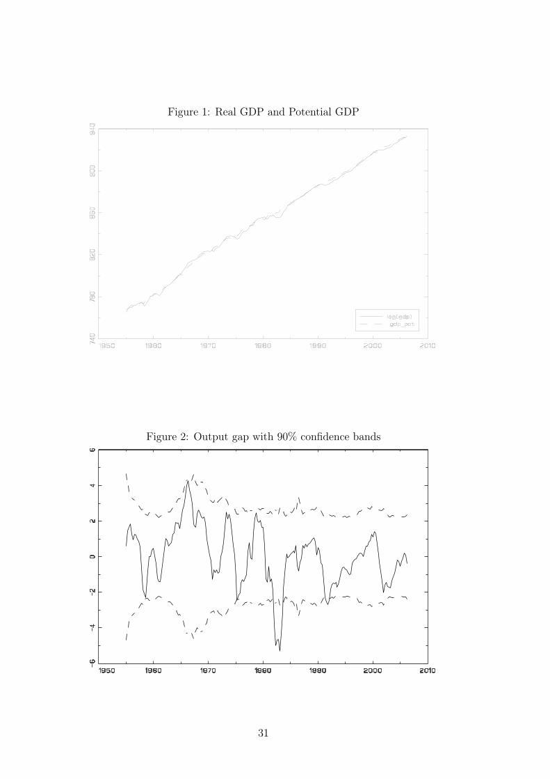
Figure 1: Real GDP and Potential GDP
Figure 2: Output gap with 90% confidence bands
31
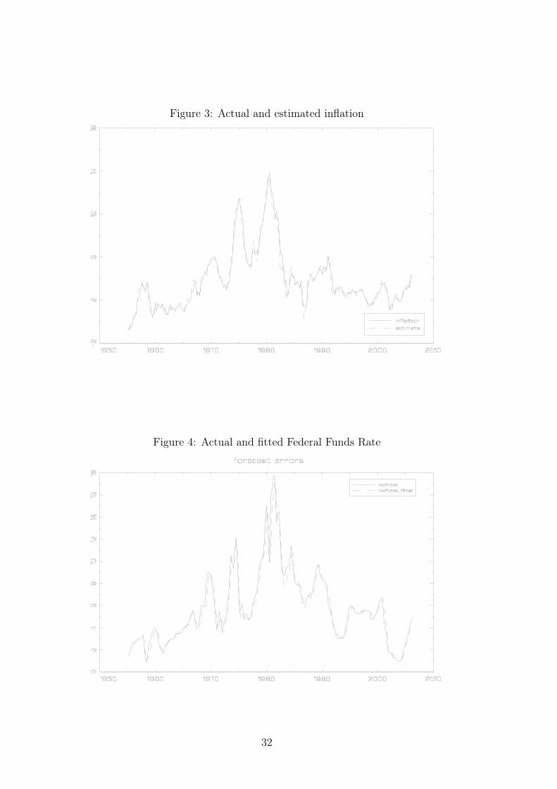
Figure 3: Actual and estimated inflation
Figure 4: Actual and fitted Federal Funds Rate
32
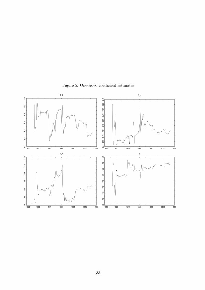
Figure 5: One-sided coefficient estimates
33
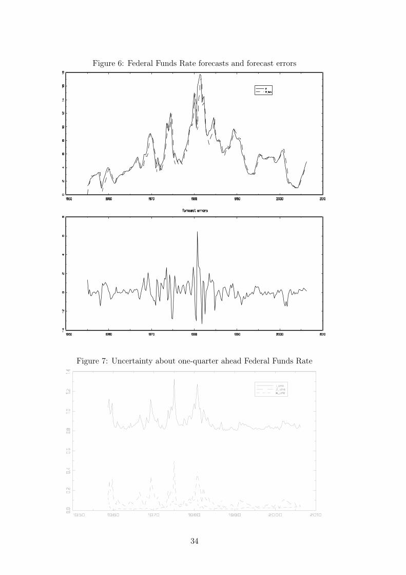
Figure 6: Federal Funds Rate forecasts and forecast errors
Figure 7: Uncertainty about one-quarter ahead Federal Funds Rate
34
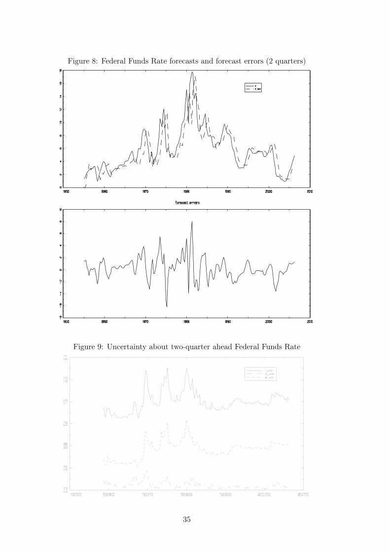
Figure 8: Federal Funds Rate forecasts and forecast errors (2 quarters)
Figure 9: Uncertainty about two-quarter ahead Federal Funds Rate
35
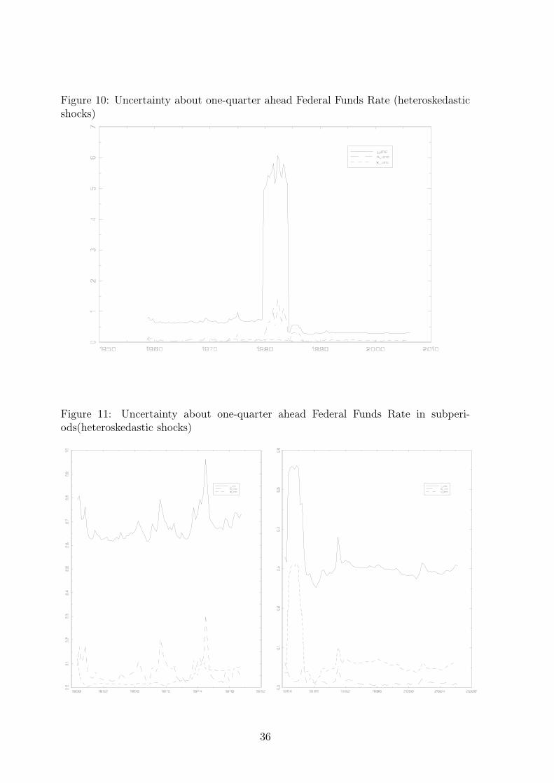
Figure 10: Uncertainty about one-quarter ahead Federal Funds Rate (heteroskedasticshocks)
Figure 11: Uncertainty about one-quarter ahead Federal Funds Rate in subperi-ods(heteroskedastic shocks)
36
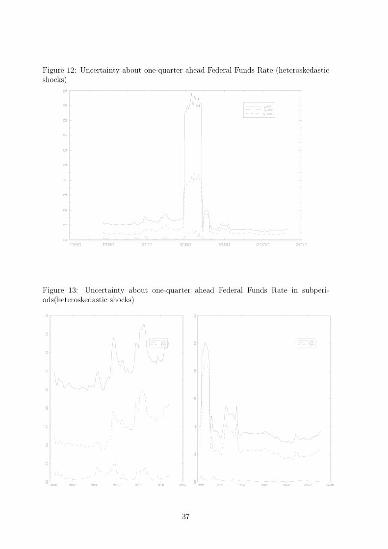
Figure 12: Uncertainty about one-quarter ahead Federal Funds Rate (heteroskedasticshocks)
Figure 13: Uncertainty about one-quarter ahead Federal Funds Rate in subperi-ods(heteroskedastic shocks)
37