the tetrahedral finite cell method for fluids
TRANSCRIPT
The tetrahedral finite cell method for fluids: Immersogeometric analysis of turbulent flowaround complex geometries
Fei Xua, Dominik Schillingerb, David Kamenskyc, Vasco Varduhnb, Chenglong Wanga, Ming-Chen Hsua,∗
aDepartment of Mechanical Engineering, Iowa State University, 2025 Black Engineering, Ames, IA 50011, USAbDepartment of Civil, Environmental, and Geo- Engineering, University of Minnesota, 500 Pillsbury Drive S.E., Minneapolis, MN 55455, USA
cInstitute for Computational Engineering and Sciences, The University of Texas at Austin, 201 East 24th St, Stop C0200, Austin, TX 78712, USA
Abstract
We present a tetrahedral finite cell method for the simulation of incompressible flow around geometrically complex objects.The method immerses such objects into non-boundary-fitted meshes of tetrahedral finite elements and weakly enforces Dirichletboundary conditions on the objects’ surfaces. Adaptively-refined quadrature rules faithfully capture the flow domain geometry inthe discrete problem without modifying the non-boundary-fitted finite element mesh. A variational multiscale formulation providesaccuracy and robustness in both laminar and turbulent flow conditions. We assess the accuracy of the method by analyzing theflow around an immersed sphere for a wide range of Reynolds numbers. We show that quantities of interest such as the dragcoefficient, Strouhal number and pressure distribution over the sphere are in very good agreement with reference values obtainedfrom standard boundary-fitted approaches. We place particular emphasis on studying the importance of the geometry resolution inintersected elements. Aligning with the immersogeometric concept, our results show that the faithful representation of the geometryin intersected elements is critical for accurate flow analysis. We demonstrate the potential of our proposed method for high-fidelityindustrial scale simulations by performing an aerodynamic analysis of an agricultural tractor.
Keywords: Immersed method, Complex geometry, Immersogeometric finite elements, Geometric accuracy in intersectedelements, Weakly enforced boundary conditions, Tetrahedral finite cell method
1. Introduction
Immersed methods approximate the solution of boundaryvalue problems on analysis meshes that do not necessarily con-form to the boundary of the domain. Such methods have greatergeometric flexibility than their boundary-fitted counterparts andcircumvent the meshing obstacles that frequently impede anal-ysis of problems posed on geometrically-complex domains. Inthe context of computational fluid dynamics (CFD), immersedmethods have a long tradition that dates back at least to theImmersed Boundary Method developed by Peskin [1] to simu-late cardiac mechanics and associated blood flow. Since then,the body of research on immersed methods area has undergonetremendous growth [2–5].
In the context of finite elements [6], several variants of im-mersed methods for fluids have been explored over the lastdecade. Lohner et al. [7–9] adapted kinetic and kinematic en-forcement of boundary conditions used in immersed bound-ary methods [5] for use in adaptive nodal finite element grids.Glowinski et al. [10–12] simulated viscous flow interactingwith rigid particles by forcing the rigid body motion in eachparticle sub-domain onto the overlapping fluid field via a dis-tributed Lagrange multiplier field. Zhang, Liu and cowork-ers [13–16] proposed the Immersed Finite Element Method
∗Corresponding authorEmail address: [email protected] (Ming-Chen Hsu)
(IFEM) to use a flexible Lagrangian solid mesh that moves ontop of a background Eulerian fluid mesh. This circumvented themajor limitation of the immersed boundary method where thefiber-like one-dimentional structure carries mass but does notoccupy volume, and opened the door to the immersed methodsfor fluid–structure interaction (FSI) problems. The concept ofIFEM was extended recently by Casquero et al. [17] to use Non-Uniform Rational B-Splines (NURBS) as the basis functions toimprove the robustness and accuracy of the immersed methodfor FSI.
In addition, several researchers designed immersed methodsthat resolve immersed boundaries and introduce weak couplingschemes for velocity and stress fields directly at the interface.Baaijens [18] and Parussini et al. [19, 20] combined the ficti-tious domain approach with Lagrange multiplier fields at theinterface for immersed thin and volumetric structures. Gersten-berger, Wall and coworkers [21–23] combined Lagrange multi-plier fields with interface enrichments of the velocity and pres-sure fields in the sense of the extended finite element methodto ensure the separation of physical and fictitious domains.Ruberg and Cirak [24, 25] combined weak Nitsche-type cou-pling methods at the interface with Cartesian B-spline finite el-ements for moving boundary and FSI problems. Several groupsalso started to work on non-boundary-fitted FSI methods, whereboth the fluid and the solid domains are immersed [26–30].
This work presents an immersed method for solving incom-pressible flow problems on unstructured tetrahedral finite el-
The final publication is available at Computers & Fluids via http://dx.doi.org/10.1016/ j.compfluid.2015.08.027
ement meshes. The proposed method combines a variationalmultiscale (VMS) formulation of incompressible flow [31–34],consistent weak enforcement of boundary conditions [35–38],and a geometrically-accurate representation of the fluid domainin the integration of the variational problem on elements thatstraddle the domain boundary. We emphasize the implicationsof the latter, highlighting the importance of accurately describ-ing the geometry in intersected elements for obtaining accu-rate flow solutions. Several studies have shown that inaccuratequadrature in elements cut by domain boundaries introduces ageometry error, which prevents higher-order accuracy of im-mersed methods [39, 40]. Influenced by isogeometric analy-sis [41, 42], which has recently drawn broader recognition tothe importance of eliminating geometric errors, we follow ourprevious work [43] in denoting immersed methods that accu-rately represent the geometry of the domain as immersogeomet-ric methods.
A pioneering instantiation of the immersogeometric con-cept is the Finite Cell Method (FCM), introduced by Parvizianet al. [44] and Duster et al. [45]. The FCM represents the geom-etry of the domain in intersected elements by adaptive quadra-ture points, such that the geometric accuracy can be increasedby adding additional levels of quadrature points, if needed. Theadaptive quadrature scheme is based on the decomposition ofeach intersected element into sub-cells that can be efficientlyorganized in hierarchical tree data structures. Although thisstrategy leads to an increased number of quadrature points inintersected elements, its implementation is extremely robustand flexible; sub-cell decomposition can operate with almostany geometric model, ranging from boundary representationsin computer aided geometric design to voxel representationsobtained from medical imaging technologies [46].
Since its inception, significant efforts have been invested tofurther develop the FCM. Technical improvements include theweak imposition of boundary and coupling conditions [47, 48],local refinement schemes [49–53], and improved quadraturerules for intersected elements [39, 40, 54]. Furthermore, theFCM has been successfully applied for large deformation anal-ysis [55, 56], thermoelasticity [57], homogenization [58], bonemechanics [59], topology optimization [60], and elastodynam-ics and wave propagation [61–63]. A concise summary of theFCM and related developments and applications can be foundin the recent review article by Schillinger and Ruess [46]. Inaddition, there exists an open-source MATLAB code1 that pro-vides an easy-to-handle starting point for running numericaltests with the FCM [64].
Most prior work on the FCM used structured meshes ofhexahedral elements, but this is not a necessary feature of theFCM. Varduhn et al. [65] recently applied the FCM with un-structured meshes of tetrahedral elements. The present contri-bution extends the tetrahedral FCM of [65] to simulations ofincompressible flow, where the flexibility of unstructured tetra-hedral meshes is useful for boundary layer refinement. One keyfeature of this study is that for all example problems consid-ered, we employ a boundary-fitted finite element method based
1http://fcmlab.cie.bgu.tum.de
on the VMS formulation with weakly enforced boundary condi-tions to compute reference solutions. Corresponding boundary-fitted and immersogeometric analyses use tetrahedral mesheswith the same refinement pattern and approximately the samenumber of degrees of freedom. Based on this comparison, weshow that our immersogeometric method achieves results thatare in very good accordance with standard boundary-fitted re-sults in terms of key quantities of interest.
This paper is organized as follows. In Section 2, we de-scribe the precise variational problem under consideration andour discrete formulation of it. Section 3 details the implemen-tation of the key technical components, including a tree basedelement decomposition for geometrically accurate quadraturein intersected elements and an efficient point-location query forinside-outside tests. Section 4 focuses on the canonical bench-mark of the flow around a sphere at Reynolds numbers of 100,300 and 3700. We compare the results of immersogeomet-ric analysis to boundary-fitted reference computations of thisbenchmark problem to demonstrate that our method accuratelycomputes quantities of interest. Section 5 presents a detailed ac-count of the accuracy of our method for the flow analysis of thefull-scale tractor, illustrating the potential of immersogeomet-ric analysis for high-fidelity aerodynamic analysis of industrial-scale problems. Section 6 draws conclusions and motivates fu-ture work.
2. Variational formulation and discretization
In this section, we summarize the variational formulationof the Navier–Stokes equations of incompressible flow and itsspatial and temporal discretizations. We also briefly review thevariational multiscale (VMS) method and the weak enforce-ment of boundary conditions. Note that the framework re-viewed in this section equally holds for immersogeometric andboundary-fitted finite element methods.
2.1. Governing equations of incompressible flow
Let Ω (subsets of Rd, d ∈ 2, 3) denote the spatial domainand Γ be its boundary. The incompressible Navier–Stokes equa-tions on Ω can be written as
ρ
(∂u∂t
+ u · ∇∇∇u − f)−∇∇∇ ·σσσ = 0 , (1)
∇∇∇ · u = 0 , (2)
where ρ, u, and f are the density of the fluid, the velocity ofthe fluid and the external force per unit mass, respectively. Thestress and strain-rate tensors are defined respectively as
σσσ (u, p) = −p I + 2µεεε(u) , (3)
εεε(u) =12
(∇∇∇u +∇∇∇uT
), (4)
where p is the pressure, I is the identity tensor and µ is the dy-namic viscosity. The problem (1)–(4) is accompanied by suit-able boundary conditions, defined on the boundary of the fluid
2
domain, Γ = ΓD ∪ ΓN :
u = g on ΓD , (5)
−p n + 2µεεε(u) n = h on ΓN , (6)
where g denotes the prescribed velocity at the Dirichlet bound-ary ΓD, h is the traction vector at the Neumann boundary ΓN ,and n is the outward unit normal.
2.2. Semi-discrete variational multiscale formulation
Consider a collection of disjoint elements Ωe, ∪eΩe ⊂ Rd,
with closures covering the fluid domain: Ω ⊂ ∪eΩe. Note thatΩe is not necessarily a subset of Ω. Let Vh
u and Vhp be the
discrete velocity and pressure spaces of functions supported onthese elements. The strong problem (1)–(6) may be recast in aweak form and posed over these discrete spaces to produce thefollowing semi-discrete problem: Find uh ∈ Vh
u and ph ∈ Vhp
such that for all wh ∈ Vhu and qh ∈ Vh
p:
BVMS(wh, qh, uh, ph
)− FVMS
(wh, qh
)= 0 . (7)
The bilinear form BVMS and the load vector FVMS are given as
BVMS(wh, qh, uh, ph
)=
∫Ω
wh · ρ
(∂uh
∂t+ uh · ∇∇∇uh
)dΩ
+
∫Ω
εεε(wh) : σσσ(uh, ph
)dΩ +
∫Ω
qh∇∇∇ · uh dΩ
−∑
e
∫Ωe∩Ω
(uh · ∇∇∇wh +
∇∇∇qh
ρ
)· u′ dΩ
−∑
e
∫Ωe∩Ω
p′∇∇∇ · wh dΩ
+∑
e
∫Ωe∩Ω
wh · (u′ · ∇∇∇uh) dΩ
−∑
e
∫Ωe∩Ω
∇∇∇wh
ρ:(u′ ⊗ u′
)dΩ
+∑
e
∫Ωe∩Ω
(u′ · ∇∇∇wh
)τ ·
(u′ · ∇∇∇uh
)dΩ , (8)
and
FVMS(wh, qh
)=
∫Ω
wh · ρ f dΩ +
∫ΓN
wh · h dΓ , (9)
where u′ is defined as
u′ = −τM
(ρ
(∂uh
∂t+ uh · ∇∇∇uh − f
)−∇∇∇ ·σσσ
(uh, ph
)), (10)
and p′ is given by
p′ = −ρ τC∇∇∇ · uh . (11)
Equations (8)–(11) emanate from the VMS formulation of theNavier–Stokes equations of incompressible flow [34]. Theterms integrated over element interiors would not appear in a
Galerkin method based on the canonical weak form of incom-pressible Navier–Stokes. These additional terms may be in-terpreted both as stabilization and as a turbulence model [32–34, 66–69]. The stabilization parameters are
τM =
( Ct
∆t2 + u ·G u + CI ν2 G : G
)−1/2
, (12)
τC = (τM tr G)−1 , (13)
τ =(u′ ·G u′
)−1/2 , (14)
where ∆t is the time-step size, CI is a positive constant de-rived from an appropriate element-wise inverse estimate [70–72], ν = µ/ρ is the kinematic viscosity, G generalizes the notionof element size to physical elements mapped from a parametricparent element by x(ξ):
Gi j =
d∑k=1
∂ξk
∂xi
∂ξk
∂x j, (15)
tr G is the trace of G, and the parameter Ct is typically equal to4 [34, 68].
Note that we allow the fluid domain boundary to intersectthe finite elements. Hence, each intersected element consists ofa fluid portion of Ωe, over which the formulation is integrated,and a portion of Ωe outside of the fluid domain, over which theintegration is discarded. The boundary Γ is discretized into anumber of surface elements. In a boundary-fitted method, theseboundary elements naturally arise as the surfaces of finite el-ements adjacent to the boundary of the fluid domain. In animmersogeometric method, surface elements are defined inde-pendently of the background finite element mesh.
2.3. Variationally consistent weak boundary conditions
The standard way of imposing Dirichlet boundary condi-tions in Eq. (7) is to enforce them strongly by ensuring that theyare satisfied by all trial solution functions. This is not feasiblein immersed methods (and not always desirable in boundary-fitted ones (see, e.g., [38])). We replace the strong enforcementby weakly enforced Dirichlet boundary conditions in the senseof Nitsche’s method [73] proposed by Bazilevs et al. [35–37].The semi-discrete problem becomes
BVMS(wh, qh, uh, ph
)− FVMS
(wh, qh
)−
∫ΓD
wh ·(−ph n + 2µεεε(uh) n
)dΓ
−
∫ΓD
(2µεεε(wh) n + qh n
)·(uh − g
)dΓ
−
∫ΓD,−
wh · ρ(uh · n
) (uh − g
)dΓ
+
∫ΓDτB
TAN
(wh −
(wh · n
)n)·((
uh − g)−
((uh − g
)· n
)n)
dΓ
+
∫ΓDτB
NOR
(wh · n
) ((uh − g
)· n
)dΓ = 0 . (16)
3
In the above equation, ΓD,− is the inflow part of ΓD, on whichuh · n < 0. The term integrated over ΓD,− increases the sta-bility of the formulation without breaking variational consis-tency [35]. τB
TAN and τBNOR are stabilization parameters that act
on the tangential and normal components of the velocity at theboundary, respectively. They need to be chosen element-wiseas a compromise between the following two requirements. Ifthey are too large, they assume a penalty-type character, affect-ing the conditioning of the stiffness matrix and overshadowingthe variational consistency. If they are too small, the solutionof Eq. (16) is unstable. Bazilevs et al. [35–37] indicate that thestabilization parameters should scale like τB
(·) = CBI µ/h, where
h has dimensions of length and indicates the element size at theboundary and CB
I is a dimensionless constant. In immersoge-ometric methods, the definitions of h and CB
I depend on howthe boundary intersects each element. References [48, 74] de-scribe a method for computing optimal stabilization parametersin each intersected element. In this work, for simplicity, we useuniform values of τB
TAN and τBNOR. These uniform values typi-
cally need to be higher than the element-wise stabilization pa-rameters computed using the methods of [48, 74]. Overestima-tion of τB
TAN may lead to excessive penalization of flow slippingalong the boundary. Although maybe counter-intuitive at firstsight, some violation of the no-slip boundary condition is in factdesirable, in particular for coarse meshes, as it imitates the pres-ence of a boundary layer [35–38, 75]. This allows for an accu-rate overall flow solution, even if the mesh size in wall-normaldirection is relatively large. Also, over-penalization of solutiondifferences between non-matching meshes tends to produce os-cillatory coupling forces, as is well-known in computationalcontact mechanics [76–80]. High-fidelity surface traction cal-culations would therefore likely benefit from the methods ofreferences [48, 74]. In the present work, though, we are prin-cipally interested in net forces on structures and turbulent flowcharacteristics, for which we found uniform penalty constantssufficient.
Remark 1. For immersogeometric methods, weakly enforcedboundary conditions are particularly attractive as the addi-tional Nitsche terms in Eq. (16) are formulated independentlyof the mesh. In contrast to strong enforcement, which relieson boundary-fitted meshes to impose Dirichlet boundary con-ditions on the discrete solution space, the Nitsche terms inEq. (16) also hold for intersected elements, where the domainboundary does not coincide with element boundaries. All that isneeded is a separate discretization of the domain boundary withindependent boundary segments whose position in intersectedelements is known or can be determined.
2.4. Time integration and iterative solution methods
We complete the discretization of Eq. (16) by a time inte-gration scheme from the family of generalized-α integrators.Generalized-α methods were introduced by Chung and Hul-bert [81] for structural dynamics and later extended to the un-steady Navier–Stokes problem by Jansen et al. [82]. The sub-set of generalized-α methods used in the current work is pa-rameterized by a single number, ρ∞, where 0 ≤ ρ∞ ≤ 1 (see
Bazilevs et al. [83] for details). Following Bazilevs et al. [34],we use ρ∞ = 0.5 for all computations presented in this paper.The generalized-α scheme is implicit and requires solution of anonlinear algebraic problem at each time step. We directly ap-ply Newton–Raphson iterations (with an approximate tangent)to converge the residual of this algebraic problem. For eachNewton–Raphson iteration, the linear system is solved using ablock-diagonal preconditioned GMRES method [84, 85].
3. Implementation of the tetrahedral finite cell method
The main challenge entailed by non-boundary-fitted meshesis the geometrically accurate evaluation of volume and surfaceintegrals in intersected elements. These integrals directly em-anate from the variational formulation (16). Our immersogeo-metric method largely draws on the FCM, which is briefly re-viewed first. Specializing to tetrahedral elements, we detail thebasic technology components, which are a volume quadraturemethod based on recursive subdivision of intersected elementsand a surface quadrature method that uses an independent sur-face mesh. In addition, we briefly describe the implementa-tion of an efficient point location query to determine whethera quadrature point is located inside or outside of the fluid do-main. We finally outline an efficient workflow for the gener-ation of immersogeometric meshes that combines our quadra-ture methods with an open-source mesh generator and locallyrefined boundary layers.
3.1. The finite cell method
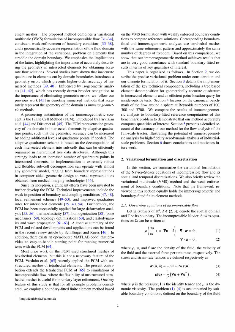
The FCM is a technique for solving partial differential equa-tions posed on complex geometries. For a summary of recentdevelopments, we refer the interested reader to [46]. The FCMis based on the fictitious domain concept illustrated in Fig. 1.Its main idea is to extend the original fluid domain to a moretractable shape, e.g., a rectangular prism bounding the origi-nal domain. The FCM discretizes the embedding domain into
Ω
ΩΩ = Ω + Ω
Γ
phys
fict
fictphys
Figure 1: The physical domain of interest Ωphys is extended by the fictitiousdomain Ωfict into an embedding domain Ω to allow easy meshing of complexgeometries. Elements without support in Ωphys can be discarded from the mesh,since they do not contribute to the solution fields in the physical domain.
4
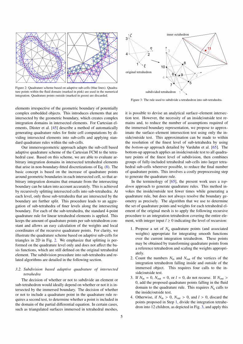
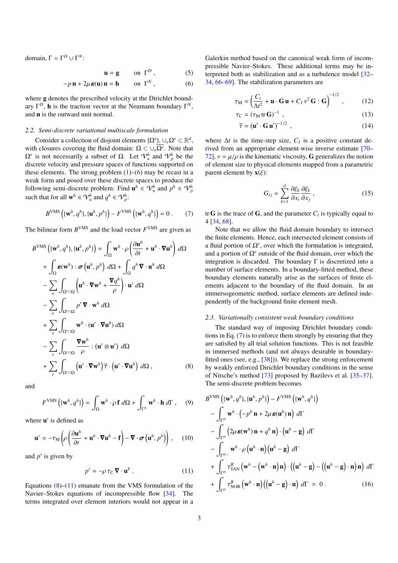
Figure 2: Quadrature scheme based on adaptive sub-cells (blue lines). Quadra-ture points within the fluid domain (marked in pink) are used in the numericalintegration. Quadrature points outside (marked in green) are discarded.
elements irrespective of the geometric boundary of potentiallycomplex embedded objects. This introduces elements that areintersected by the geometric boundary, which creates complexintegration domains in intersected elements. For Cartesian el-ements, Duster et al. [45] describe a method of automaticallygenerating quadrature rules for finite cell computations by di-viding intersected elements into sub-cells and applying stan-dard quadrature rules within the sub-cells.
Our immersogeometric approach adapts the sub-cell basedadaptive quadrature scheme of the Cartesian FCM to the tetra-hedral case. Based on this scheme, we are able to evaluate ar-bitrary integration domains in intersected tetrahedral elementsthat arise in non-boundary-fitted discretizations of Eq. (8). Thebasic concept is based on the increase of quadrature pointsaround geometric boundaries in each intersected cell, so that ar-bitrary integration domains that emanate from the intersectingboundary can be taken into account accurately. This is achievedby recursively splitting intersected cells into sub-tetrahedra. Ateach level, only those sub-tetrahedra that are intersected by theboundary are further split. This procedure leads to an aggre-gation of sub-tetrahedra of finer levels along the intersectingboundary. For each of the sub-tetrahedra, the standard 4-pointquadrature rule for linear tetrahedral elements is applied. Thiskeeps the amount of quadrature points per sub-tetrahedron con-stant and allows an easy calculation of the weights and localcoordinates of the recursive quadrature points. For clarity, weillustrate the quadrature scheme based on adaptive sub-cells fortriangles in 2D in Fig. 2. We emphasize that splitting is per-formed on the quadrature level only and does not affect the ba-sis functions, which are still defined on the original tetrahedralelement. The subdivision procedure into sub-tetrahedra and re-lated algorithms are detailed in the following section.
3.2. Subdivision based adaptive quadrature of intersectedtetrahedra
The decision of whether or not to subdivide an element orsub-tetrahedron would ideally depend on whether or not it is in-tersected by the immersed boundary. The decision of whetheror not to include a quadrature point in the quadrature rule re-quires a second test, to determine whether a point is included inthe domain of the partial differential equation. In certain cases,such as triangulated surfaces immersed in tetrahedral meshes,
11
7 5
810
6 9
1
2
3
4
subdivided tetrahedron
inner octahedron
4
1
2
3
ξ
η
ζ
original tetrahedron
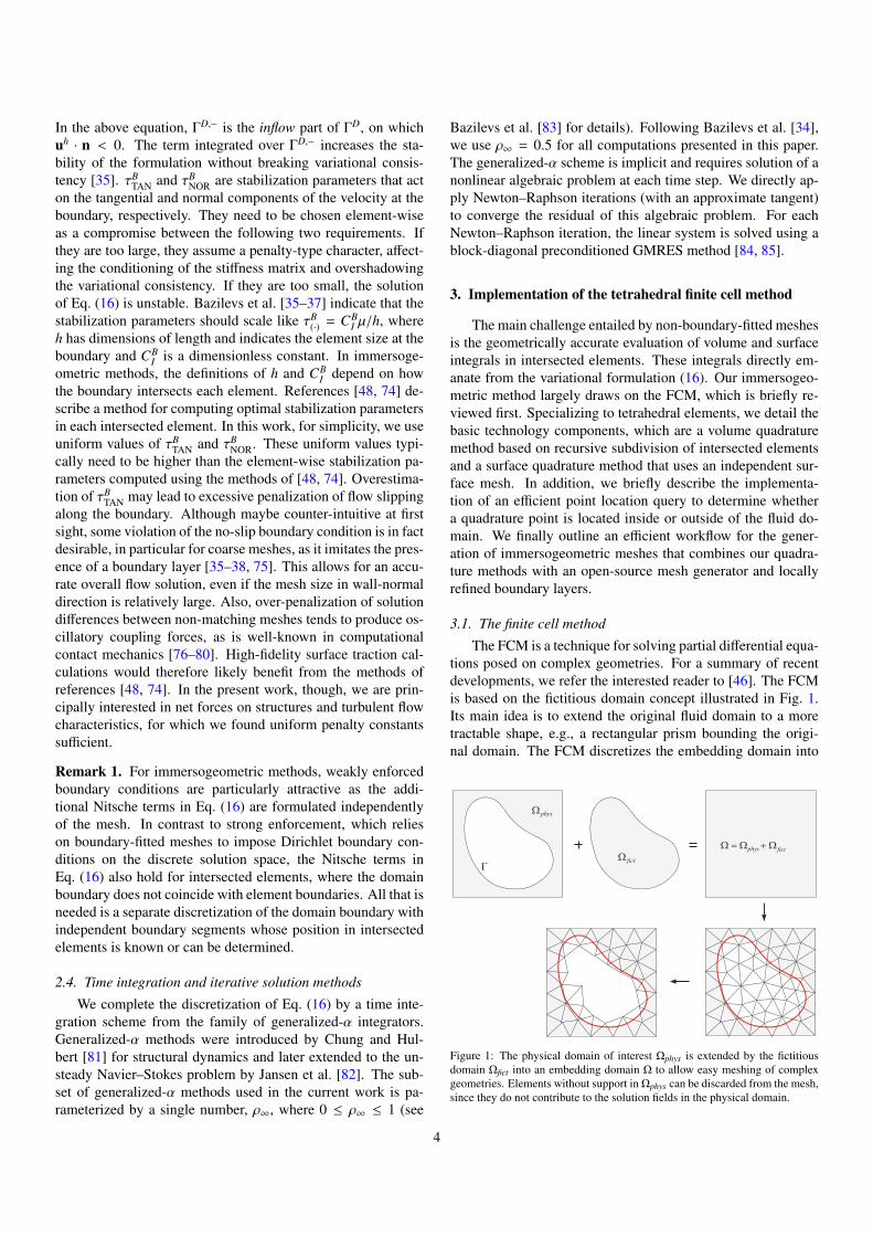
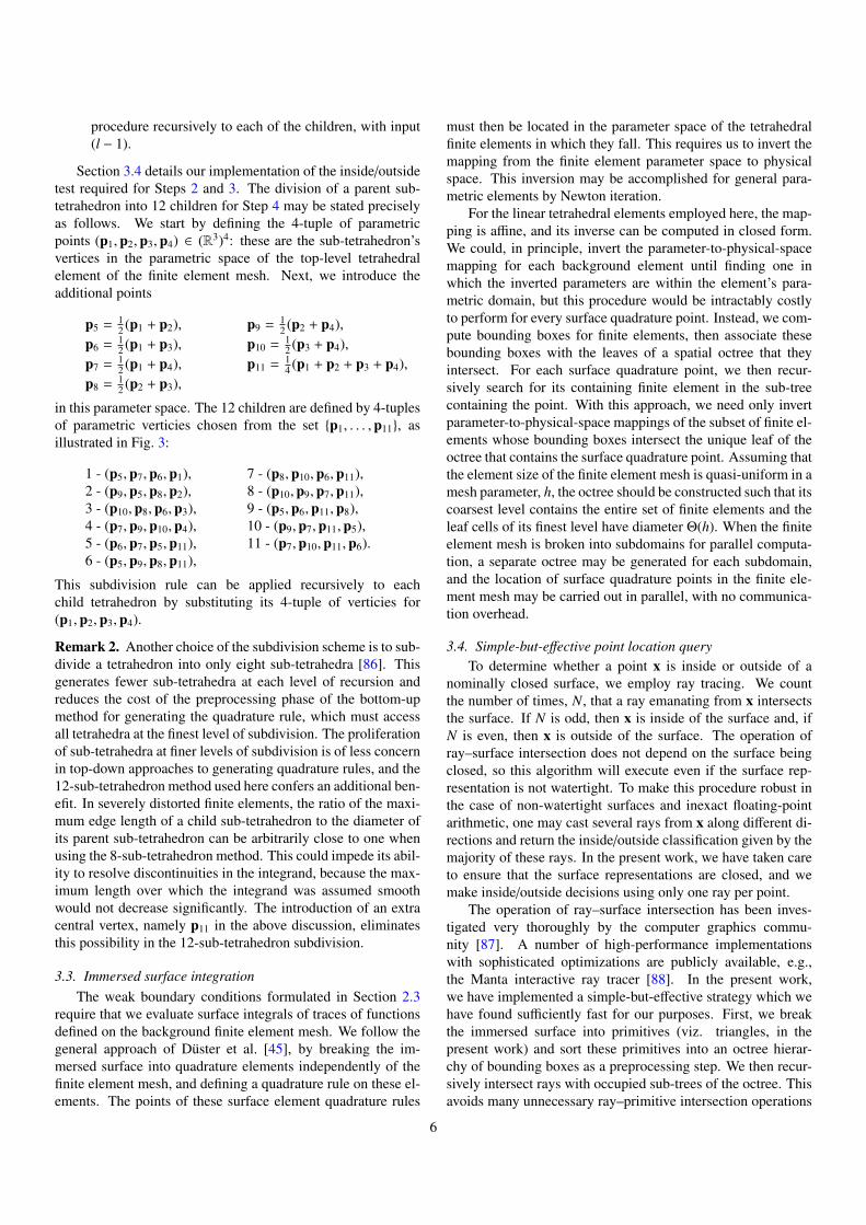
Figure 3: The rule used to subdivide a tetrahedron into sub-tetrahedra.
it is possible to devise an analytical surface–element intersec-tion test. However, the necessity of an inside/outside test re-mains and, to reduce the number of assumptions required ofthe immersed boundary representation, we propose to approx-imate the surface–element intersection test using only the in-side/outside test. This approximation can be made to withinthe resolution of the finest level of sub-tetrahedra by usingthe bottom-up approach detailed by Varduhn et al. [65]. Thebottom-up approach applies an inside/outside test to all quadra-ture points of the finest level of subdivision, then combinesgroups of fully-included tetrahedral sub-cells into larger tetra-hedral sub-cells wherever possible, to reduce the final numberof quadrature points. This involves a costly preprocessing stepto generate the quadrature rule.
In the terminology of [65], the present work uses a top-down approach to generate quadrature rules. This method in-vokes the inside/outside test fewer times while generating aquadrature rule, but does not always resolve the boundary ge-ometry as precisely. The algorithm that we use to determinethe set of quadrature points and weights for each tetrahedral el-ement of the original mesh is to apply the following recursiveprocedure to an integration tetrahedron covering the entire ele-ment, with integer input l ≥ 0 indicating the level of recursion:
1. Propose a set of Nq quadrature points (and associatedweights) appropriate for integrating smooth functionsover the current integration tetrahedron. These pointsmay be obtained by transforming quadrature points froma reference tetrahedron and scaling the weights appropri-ately.
2. Count the numbers Nin and Nout of the vertices of theintegration tetrahedron falling inside and outside of theimmersed object. This requires four calls to the in-side/outside test.
3. If Nin = 0, Nout = 0, or l = 0, do not recurse. If Nout >0, add the proposed quadrature points falling in the fluiddomain to the quadrature rule. This requires Nq calls tothe inside/outside test.
4. Otherwise, if Nin > 0, Nout > 0, and l > 0, discard thepoints proposed in Step 1, divide the integration tetrahe-dron into 12 children, as depicted in Fig. 3, and apply this
5
procedure recursively to each of the children, with input(l − 1).
Section 3.4 details our implementation of the inside/outsidetest required for Steps 2 and 3. The division of a parent sub-tetrahedron into 12 children for Step 4 may be stated preciselyas follows. We start by defining the 4-tuple of parametricpoints (p1,p2,p3,p4) ∈ (R3)4: these are the sub-tetrahedron’svertices in the parametric space of the top-level tetrahedralelement of the finite element mesh. Next, we introduce theadditional points
p5 = 12 (p1 + p2), p9 = 1
2 (p2 + p4),p6 = 1
2 (p1 + p3), p10 = 12 (p3 + p4),
p7 = 12 (p1 + p4), p11 = 1
4 (p1 + p2 + p3 + p4),p8 = 1
2 (p2 + p3),
in this parameter space. The 12 children are defined by 4-tuplesof parametric verticies chosen from the set p1, . . . ,p11, asillustrated in Fig. 3:
1 - (p5,p7,p6,p1), 7 - (p8,p10,p6,p11),2 - (p9,p5,p8,p2), 8 - (p10,p9,p7,p11),3 - (p10,p8,p6,p3), 9 - (p5,p6,p11,p8),4 - (p7,p9,p10,p4), 10 - (p9,p7,p11,p5),5 - (p6,p7,p5,p11), 11 - (p7,p10,p11,p6).6 - (p5,p9,p8,p11),
This subdivision rule can be applied recursively to eachchild tetrahedron by substituting its 4-tuple of verticies for(p1,p2,p3,p4).
Remark 2. Another choice of the subdivision scheme is to sub-divide a tetrahedron into only eight sub-tetrahedra [86]. Thisgenerates fewer sub-tetrahedra at each level of recursion andreduces the cost of the preprocessing phase of the bottom-upmethod for generating the quadrature rule, which must accessall tetrahedra at the finest level of subdivision. The proliferationof sub-tetrahedra at finer levels of subdivision is of less concernin top-down approaches to generating quadrature rules, and the12-sub-tetrahedron method used here confers an additional ben-efit. In severely distorted finite elements, the ratio of the maxi-mum edge length of a child sub-tetrahedron to the diameter ofits parent sub-tetrahedron can be arbitrarily close to one whenusing the 8-sub-tetrahedron method. This could impede its abil-ity to resolve discontinuities in the integrand, because the max-imum length over which the integrand was assumed smoothwould not decrease significantly. The introduction of an extracentral vertex, namely p11 in the above discussion, eliminatesthis possibility in the 12-sub-tetrahedron subdivision.
3.3. Immersed surface integrationThe weak boundary conditions formulated in Section 2.3
require that we evaluate surface integrals of traces of functionsdefined on the background finite element mesh. We follow thegeneral approach of Duster et al. [45], by breaking the im-mersed surface into quadrature elements independently of thefinite element mesh, and defining a quadrature rule on these el-ements. The points of these surface element quadrature rules
must then be located in the parameter space of the tetrahedralfinite elements in which they fall. This requires us to invert themapping from the finite element parameter space to physicalspace. This inversion may be accomplished for general para-metric elements by Newton iteration.
For the linear tetrahedral elements employed here, the map-ping is affine, and its inverse can be computed in closed form.We could, in principle, invert the parameter-to-physical-spacemapping for each background element until finding one inwhich the inverted parameters are within the element’s para-metric domain, but this procedure would be intractably costlyto perform for every surface quadrature point. Instead, we com-pute bounding boxes for finite elements, then associate thesebounding boxes with the leaves of a spatial octree that theyintersect. For each surface quadrature point, we then recur-sively search for its containing finite element in the sub-treecontaining the point. With this approach, we need only invertparameter-to-physical-space mappings of the subset of finite el-ements whose bounding boxes intersect the unique leaf of theoctree that contains the surface quadrature point. Assuming thatthe element size of the finite element mesh is quasi-uniform in amesh parameter, h, the octree should be constructed such that itscoarsest level contains the entire set of finite elements and theleaf cells of its finest level have diameter Θ(h). When the finiteelement mesh is broken into subdomains for parallel computa-tion, a separate octree may be generated for each subdomain,and the location of surface quadrature points in the finite ele-ment mesh may be carried out in parallel, with no communica-tion overhead.
3.4. Simple-but-effective point location queryTo determine whether a point x is inside or outside of a
nominally closed surface, we employ ray tracing. We countthe number of times, N, that a ray emanating from x intersectsthe surface. If N is odd, then x is inside of the surface and, ifN is even, then x is outside of the surface. The operation ofray–surface intersection does not depend on the surface beingclosed, so this algorithm will execute even if the surface rep-resentation is not watertight. To make this procedure robust inthe case of non-watertight surfaces and inexact floating-pointarithmetic, one may cast several rays from x along different di-rections and return the inside/outside classification given by themajority of these rays. In the present work, we have taken careto ensure that the surface representations are closed, and wemake inside/outside decisions using only one ray per point.
The operation of ray–surface intersection has been inves-tigated very thoroughly by the computer graphics commu-nity [87]. A number of high-performance implementationswith sophisticated optimizations are publicly available, e.g.,the Manta interactive ray tracer [88]. In the present work,we have implemented a simple-but-effective strategy which wehave found sufficiently fast for our purposes. First, we breakthe immersed surface into primitives (viz. triangles, in thepresent work) and sort these primitives into an octree hierar-chy of bounding boxes as a preprocessing step. We then recur-sively intersect rays with occupied sub-trees of the octree. Thisavoids many unnecessary ray–primitive intersection operations
6
relative to the brute force approach of testing each ray againsteach surface primitive.
3.5. Generating adaptive non-boundary-fitted meshesThe immersogeometric concept based on the FCM is in-
dependent of a specific basis and can be used with any basisfunction technology and element type. The main motivation forusing tetrahedral elements is their ability to provide locally re-fined three-dimensional discretizations, which is required herefor boundary layer resolution. In contrast to hexahedral el-ements, there exist generally valid refinement algorithms fortetrahedra that work in any situation without restrictions. Theavailability of a large number of advanced tetrahedral meshingtools [89] motivates the integration of such a tool to generatean initial unstructured tetrahedral mesh. In many immersedsituations, conforming to the boundary of a simple geometry(e.g., a rectangular box as the embedding domain) is the onlyrestricting requirement for generating a mesh; the discretiza-tion process is extremely fast, even for a very large number ofelements. At the same time, we can make use of advanced al-gorithms for mesh regularization and smoothing to ensure high-quality tetrahedral elements. We present a workflow based onan open-source mesh generator Gmsh [90] to efficiently gener-ate non-boundary-fitted adaptive tetrahedral meshes.
In immersogeometric analysis, the whole embedding do-main, including physical and fictitious domain, is discretizedirrespective of the immersed boundary. The actual geometryof the immersed object is not explicitly needed for the meshgeneration. Instead, one only needs to specify how the meshshould be graded in terms of element size over the embeddingdomain, with finer element sizes in the area of boundary layers.Gmsh enables control of the local mesh size via special func-tions that can be used in the input script. The functions we useinclude “Point”, “Attractor”, “Threshold”, “Box”, and “Min”.“Point” specifies the location where a specific mesh size will beenforced. “Attractor” specifies the mesh size within a “Thresh-old” distance to a geometrical entity such as “Point”. We usethese functions to set the element sizes in the vicinity of the im-mersed boundary. Since elements can arbitrarily intersect withthe immersed boundary, that is, the mesh conformity does notneed to be enforced, this procedure is significantly less demand-ing and much more reliable than conforming mesh generation.In addition, we use “Box” to specify the element size inside ofa parallelepiped to locally (and uniformly) refine zones wherethe flow is expected to be more complex. Finally, when sev-eral mesh size control functions are active at the same location,“Min” is used to resolve this overconstraint by choosing themesh size to be the minimum of the sizes specified in thosefunctions. For more details of the Gmsh functions, the reader isreferred to [90].
4. Benchmark example: Flow around a sphere
The flow around a sphere at Reynolds numbers Re = 100and 300 for laminar flow and Re = 3700 for turbulent flow con-stitute canonical test cases, for which a large number of refer-ence results are available in the literature (see, e.g., [91–95] for
10
10
10 20
Lateral wall
(no penetration)
2.5 10
5
1.25 6
2.5 d=1
Outer box
Outer
refinement box Inner
refinement box
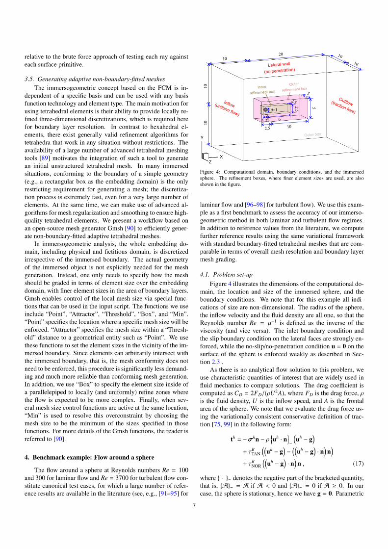
Figure 4: Computational domain, boundary conditions, and the immersedsphere. The refinement boxes, where finer element sizes are used, are alsoshown in the figure.
laminar flow and [96–98] for turbulent flow). We use this exam-ple as a first benchmark to assess the accuracy of our immerso-geometric method in both laminar and turbulent flow regimes.In addition to reference values from the literature, we computefurther reference results using the same variational frameworkwith standard boundary-fitted tetrahedral meshes that are com-parable in terms of overall mesh resolution and boundary layermesh grading.
4.1. Problem set-upFigure 4 illustrates the dimensions of the computational do-
main, the location and size of the immersed sphere, and theboundary conditions. We note that for this example all indi-cations of size are non-dimensional. The radius of the sphere,the inflow velocity and the fluid density are all one, so that theReynolds number Re = µ−1 is defined as the inverse of theviscosity (and vice versa). The inlet boundary condition andthe slip boundary condition on the lateral faces are strongly en-forced, while the no-slip/no-penetration condition u = 0 on thesurface of the sphere is enforced weakly as described in Sec-tion 2.3 .
As there is no analytical flow solution to this problem, weuse characteristic quantities of interest that are widely used influid mechanics to compare solutions. The drag coefficient iscomputed as CD = 2FD/(ρU2A), where FD is the drag force, ρis the fluid density, U is the inflow speed, and A is the frontalarea of the sphere. We note that we evaluate the drag force us-ing the variationally consistent conservative definition of trac-tion [75, 99] in the following form:
th = −σσσhn − ρuh · n
−
(uh − g
)+ τB
TAN
((uh − g
)−
((uh − g
)· n
)n)
+ τBNOR
((uh − g
)· n
)n , (17)
where · − denotes the negative part of the bracketed quantity,that is, A− = A if A < 0 and A− = 0 if A ≥ 0. In ourcase, the sphere is stationary, hence we have g = 0. Parametric
7
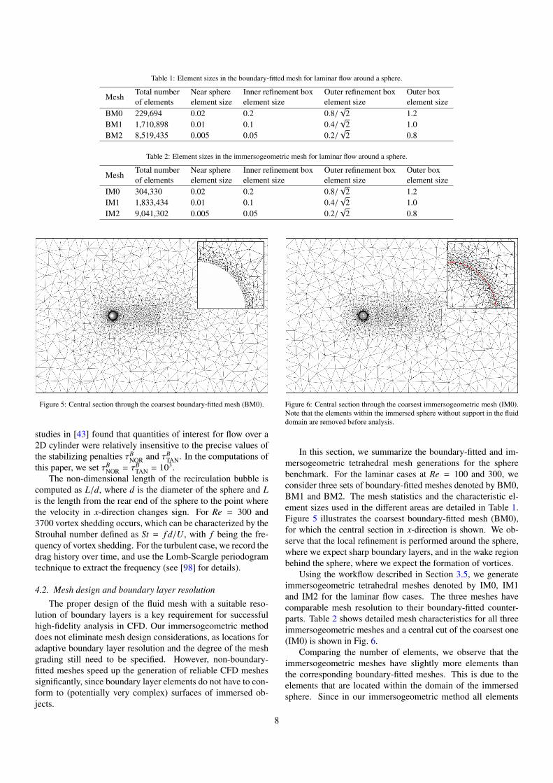
Table 1: Element sizes in the boundary-fitted mesh for laminar flow around a sphere.
MeshTotal numberof elements
Near sphereelement size
Inner refinement boxelement size
Outer refinement boxelement size
Outer boxelement size
BM0 229,694 0.02 0.2 0.8/√
2 1.2BM1 1,710,898 0.01 0.1 0.4/
√2 1.0
BM2 8,519,435 0.005 0.05 0.2/√
2 0.8
Table 2: Element sizes in the immersogeometric mesh for laminar flow around a sphere.
MeshTotal numberof elements
Near sphereelement size
Inner refinement boxelement size
Outer refinement boxelement size
Outer boxelement size
IM0 304,330 0.02 0.2 0.8/√
2 1.2IM1 1,833,434 0.01 0.1 0.4/
√2 1.0
IM2 9,041,302 0.005 0.05 0.2/√
2 0.8
Figure 5: Central section through the coarsest boundary-fitted mesh (BM0).
studies in [43] found that quantities of interest for flow over a2D cylinder were relatively insensitive to the precise values ofthe stabilizing penalties τB
NOR and τBTAN. In the computations of
this paper, we set τBNOR = τB
TAN = 103.The non-dimensional length of the recirculation bubble is
computed as L/d, where d is the diameter of the sphere and Lis the length from the rear end of the sphere to the point wherethe velocity in x-direction changes sign. For Re = 300 and3700 vortex shedding occurs, which can be characterized by theStrouhal number defined as St = f d/U, with f being the fre-quency of vortex shedding. For the turbulent case, we record thedrag history over time, and use the Lomb-Scargle periodogramtechnique to extract the frequency (see [98] for details).
4.2. Mesh design and boundary layer resolution
The proper design of the fluid mesh with a suitable reso-lution of boundary layers is a key requirement for successfulhigh-fidelity analysis in CFD. Our immersogeometric methoddoes not eliminate mesh design considerations, as locations foradaptive boundary layer resolution and the degree of the meshgrading still need to be specified. However, non-boundary-fitted meshes speed up the generation of reliable CFD meshessignificantly, since boundary layer elements do not have to con-form to (potentially very complex) surfaces of immersed ob-jects.
Figure 6: Central section through the coarsest immersogeometric mesh (IM0).Note that the elements within the immersed sphere without support in the fluiddomain are removed before analysis.
In this section, we summarize the boundary-fitted and im-mersogeometric tetrahedral mesh generations for the spherebenchmark. For the laminar cases at Re = 100 and 300, weconsider three sets of boundary-fitted meshes denoted by BM0,BM1 and BM2. The mesh statistics and the characteristic el-ement sizes used in the different areas are detailed in Table 1.Figure 5 illustrates the coarsest boundary-fitted mesh (BM0),for which the central section in x-direction is shown. We ob-serve that the local refinement is performed around the sphere,where we expect sharp boundary layers, and in the wake regionbehind the sphere, where we expect the formation of vortices.
Using the workflow described in Section 3.5, we generateimmersogeometric tetrahedral meshes denoted by IM0, IM1and IM2 for the laminar flow cases. The three meshes havecomparable mesh resolution to their boundary-fitted counter-parts. Table 2 shows detailed mesh characteristics for all threeimmersogeometric meshes and a central cut of the coarsest one(IM0) is shown in Fig. 6.
Comparing the number of elements, we observe that theimmersogeometric meshes have slightly more elements thanthe corresponding boundary-fitted meshes. This is due to theelements that are located within the domain of the immersedsphere. Since in our immersogeometric method all elements
8
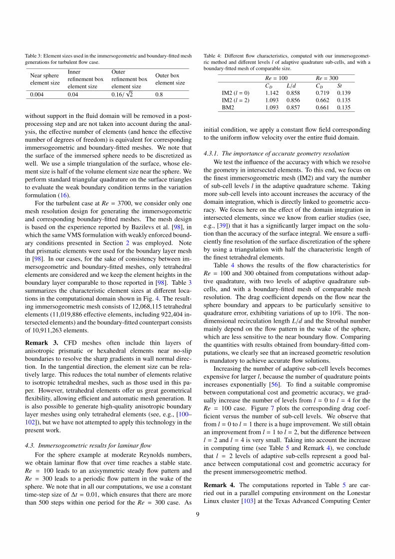
Table 3: Element sizes used in the immersogeometric and boundary-fitted meshgenerations for turbulent flow case.
Near sphereelement size
Innerrefinement boxelement size
Outerrefinement boxelement size
Outer boxelement size
0.004 0.04 0.16/√
2 0.8
without support in the fluid domain will be removed in a post-processing step and are not taken into account during the anal-ysis, the effective number of elements (and hence the effectivenumber of degrees of freedom) is equivalent for correspondingimmersogeometric and boundary-fitted meshes. We note thatthe surface of the immersed sphere needs to be discretized aswell. We use a simple triangulation of the surface, whose ele-ment size is half of the volume element size near the sphere. Weperform standard triangular quadrature on the surface trianglesto evaluate the weak boundary condition terms in the variationformulation (16).
For the turbulent case at Re = 3700, we consider only onemesh resolution design for generating the immersogeometricand corresponding boundary-fitted meshes. The mesh designis based on the experience reported by Bazilevs et al. [98], inwhich the same VMS formulation with weakly enforced bound-ary conditions presented in Section 2 was employed. Notethat prismatic elements were used for the boundary layer meshin [98]. In our cases, for the sake of consistency between im-mersogeometric and boundary-fitted meshes, only tetrahedralelements are considered and we keep the element heights in theboundary layer comparable to those reported in [98]. Table 3summarizes the characteristic element sizes at different loca-tions in the computational domain shown in Fig. 4. The result-ing immersogeometric mesh consists of 12,068,115 tetrahedralelements (11,019,886 effective elements, including 922,404 in-tersected elements) and the boundary-fitted counterpart consistsof 10,911,263 elements.
Remark 3. CFD meshes often include thin layers ofanisotropic prismatic or hexahedral elements near no-slipboundaries to resolve the sharp gradients in wall normal direc-tion. In the tangential direction, the element size can be rela-tively large. This reduces the total number of elements relativeto isotropic tetrahedral meshes, such as those used in this pa-per. However, tetrahedral elements offer us great geometricalflexibility, allowing efficient and automatic mesh generation. Itis also possible to generate high-quality anisotropic boundarylayer meshes using only tetrahedral elements (see, e.g., [100–102]), but we have not attempted to apply this technology in thepresent work.
4.3. Immersogeometric results for laminar flowFor the sphere example at moderate Reynolds numbers,
we obtain laminar flow that over time reaches a stable state.Re = 100 leads to an axisymmetric steady flow pattern andRe = 300 leads to a periodic flow pattern in the wake of thesphere. We note that in all our computations, we use a constanttime-step size of ∆t = 0.01, which ensures that there are morethan 500 steps within one period for the Re = 300 case. As
Table 4: Different flow characteristics, computed with our immersogeomet-ric method and different levels l of adaptive quadrature sub-cells, and with aboundary-fitted mesh of comparable size.
Re = 100 Re = 300CD L/d CD St
IM2 (l = 0) 1.142 0.858 0.719 0.139IM2 (l = 2) 1.093 0.856 0.662 0.135BM2 1.093 0.857 0.661 0.135
initial condition, we apply a constant flow field correspondingto the uniform inflow velocity over the entire fluid domain.
4.3.1. The importance of accurate geometry resolutionWe test the influence of the accuracy with which we resolve
the geometry in intersected elements. To this end, we focus onthe finest immersogeometric mesh (IM2) and vary the numberof sub-cell levels l in the adaptive quadrature scheme. Takingmore sub-cell levels into account increases the accuracy of thedomain integration, which is directly linked to geometric accu-racy. We focus here on the effect of the domain integration inintersected elements, since we know from earlier studies (see,e.g., [39]) that it has a significantly larger impact on the solu-tion than the accuracy of the surface integral. We ensure a suffi-ciently fine resolution of the surface discretization of the sphereby using a triangulation with half the characteristic length ofthe finest tetrahedral elements.
Table 4 shows the results of the flow characteristics forRe = 100 and 300 obtained from computations without adap-tive quadrature, with two levels of adaptive quadrature sub-cells, and with a boundary-fitted mesh of comparable meshresolution. The drag coefficient depends on the flow near thesphere boundary and appears to be particularly sensitive toquadrature error, exhibiting variations of up to 10%. The non-dimensional recirculation length L/d and the Strouhal numbermainly depend on the flow pattern in the wake of the sphere,which are less sensitive to the near boundary flow. Comparingthe quantities with results obtained from boundary-fitted com-putations, we clearly see that an increased geometric resolutionis mandatory to achieve accurate flow solutions.
Increasing the number of adaptive sub-cell levels becomesexpensive for larger l, because the number of quadrature pointsincreases exponentially [56]. To find a suitable compromisebetween computational cost and geometric accuracy, we grad-ually increase the number of levels from l = 0 to l = 4 for theRe = 100 case. Figure 7 plots the corresponding drag coef-ficient versus the number of sub-cell levels. We observe thatfrom l = 0 to l = 1 there is a huge improvement. We still obtainan improvement from l = 1 to l = 2, but the difference betweenl = 2 and l = 4 is very small. Taking into account the increasein computing time (see Table 5 and Remark 4), we concludethat l = 2 levels of adaptive sub-cells represent a good bal-ance between computational cost and geometric accuracy forthe present immersogeometric method.
Remark 4. The computations reported in Table 5 are car-ried out in a parallel computing environment on the LonestarLinux cluster [103] at the Texas Advanced Computing Center
9
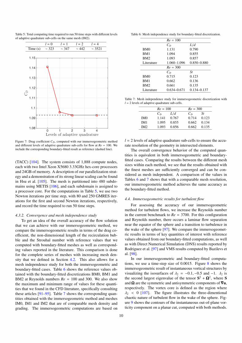
Table 5: Total computing time required to run 50 time steps with different levelsof adaptive quadrature sub-cells on the same mesh (IM2).
l = 0 l = 1 l = 2 l = 4Time (s) ∼ 323 ∼ 347 ∼ 442 ∼ 3521
Levels of adaptive quadrature0 1 2 3 4
CD
1.08
1.09
1.1
1.11
1.12
1.13
1.14
1.15
Figure 7: Drag coefficient CD, computed with our immersogeometric methodand different levels of adaptive quadrature sub-cells for flow at Re = 100. Weinclude the corresponding boundary-fitted result as reference (dashed line).
(TACC) [104]. The system consists of 1,888 compute nodes,each with two Intel Xeon X5680 3.33GHz hex-core processorsand 24GB of memory. A description of our parallelization strat-egy and a demonstration of its strong linear scaling can be foundin Hsu et al. [105]. The mesh is partitioned into 480 subdo-mains using METIS [106], and each subdomain is assigned toa processor core. For the computations in Table 5, we use twoNewton iterations per time step, with 80 and 250 GMRES iter-ations for the first and second Newton iterations, respectively,and record the time required to run 50 time steps.
4.3.2. Convergence and mesh independence studyTo get an idea of the overall accuracy of the flow solution
that we can achieve with our immersogeometric method, wecompare the immersogeometric results in terms of the drag co-efficient, the non-dimensional length of the recirculation bub-ble and the Strouhal number with reference values that wecomputed with boundary-fitted meshes as well as correspond-ing values reported in the literature. This comparison is donefor the complete series of meshes with increasing mesh den-sity that we defined in Section 4.2. This also allows for amesh independence study for both the immersogeometric andboundary-fitted cases. Table 6 shows the reference values ob-tained with the boundary-fitted discretizations BM0, BM1 andBM2 at Reynolds numbers Re = 100 and 300. We also showthe maximum and minimum range of values for these quanti-ties that we found in the CFD literature, specifically consultingthese articles [91–95]. Table 7 shows the corresponding quan-tities obtained with the immersogeometric method and meshesIM0, IM1 and IM2 that are of comparable mesh density andgrading. The immersogeometric computations are based on
Table 6: Mesh independence study for boundary-fitted discretization.
Re = 100CD L/d
BM0 1.131 0.790BM1 1.094 0.855BM2 1.093 0.857Literature 1.060–1.096 0.850–0.880
Re = 300CD St
BM0 0.715 0.123BM1 0.662 0.136BM2 0.661 0.135Literature 0.634–0.671 0.134–0.137
Table 7: Mesh independence study for immersogeometric discretization withl = 2 levels of adaptive quadrature sub-cells.
Re = 100 Re = 300CD L/d CD St
IM0 1.141 0.767 0.714 0.123IM1 1.095 0.855 0.662 0.134IM2 1.093 0.856 0.662 0.135
l = 2 levels of adaptive quadrature sub-cells to ensure the accu-rate resolution of the geometry in intersected elements.
The overall convergence behavior of the computed quan-tities is equivalent in both immersogeometric and boundary-fitted cases. Comparing the results between the different meshsizes within each method, we see that the results obtained withthe finest meshes are sufficiently converged and can be con-sidered as mesh independent. A comparison of the values inTables 6 and 7 shows that with a comparable mesh resolution,our immersogeometric method achieves the same accuracy asthe boundary-fitted method.
4.4. Immersogeometric results for turbulent flow
For assessing the accuracy of our immersogeometricmethod for turbulent flows, we increase the Reynolds numberin the current benchmark to Re = 3700. For this configurationand Reynolds number, there occurs a laminar flow separationnear the equator of the sphere and a transition to turbulence inthe wake of the sphere [97]. We compare the immersogeomet-ric results in terms of key quantities of interest with referencevalues obtained from our boundary-fitted computations, as wellas with Direct Numerical Simulation (DNS) results reported byRodriguez et al. [97] and VMS results computed by Bazilevs etal. [98].
In our immersogeometric and boundary-fitted computa-tions, we use a time-step size of 0.0015. Figure 8 shows theimmersogeometric result of instantaneous vortical structures byvisualizing the isosurfaces of λ2 = −0.1,−0.5 and −1. λ2 isthe second largest eigenvalue of the tensor S2 + ΩΩΩ2, where Sand ΩΩΩ are the symmetric and antisymmetric components of∇∇∇u,respectively. The vortex core is defined as the region whereλ2 < 0 [107]. The figure illustrates the three-dimentionalchaotic nature of turbulent flow in the wake of the sphere. Fig-ure 9 shows the contours of the instantaneous out-of-plane vor-ticity component on a planar cut, computed with both methods.
10
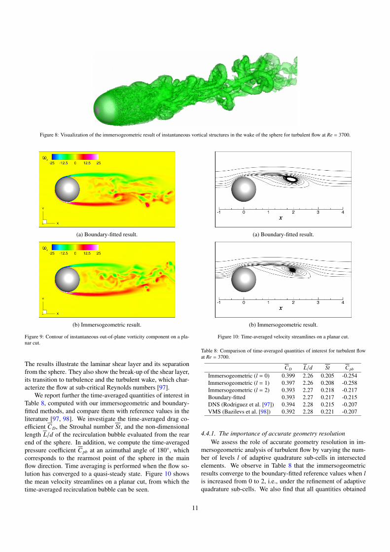
Figure 8: Visualization of the immersogeometric result of instantaneous vortical structures in the wake of the sphere for turbulent flow at Re = 3700.
(a) Boundary-fitted result.
(b) Immersogeometric result.
Figure 9: Contour of instantaneous out-of-plane vorticity component on a pla-nar cut.
The results illustrate the laminar shear layer and its separationfrom the sphere. They also show the break-up of the shear layer,its transition to turbulence and the turbulent wake, which char-acterize the flow at sub-critical Reynolds numbers [97].
We report further the time-averaged quantities of interest inTable 8, computed with our immersogeometric and boundary-fitted methods, and compare them with reference values in theliterature [97, 98]. We investigate the time-averaged drag co-efficient CD, the Strouhal number St, and the non-dimensionallength L/d of the recirculation bubble evaluated from the rearend of the sphere. In addition, we compute the time-averagedpressure coefficient Cpb at an azimuthal angle of 180, whichcorresponds to the rearmost point of the sphere in the mainflow direction. Time averaging is performed when the flow so-lution has converged to a quasi-steady state. Figure 10 showsthe mean velocity streamlines on a planar cut, from which thetime-averaged recirculation bubble can be seen.
(a) Boundary-fitted result.
(b) Immersogeometric result.
Figure 10: Time-averaged velocity streamlines on a planar cut.
Table 8: Comparison of time-averaged quantities of interest for turbulent flowat Re = 3700.
CD L/d St Cpb
Immersogeometric (l = 0) 0.399 2.26 0.205 -0.254Immersogeometric (l = 1) 0.397 2.26 0.208 -0.258Immersogeometric (l = 2) 0.393 2.27 0.218 -0.217Boundary-fitted 0.393 2.27 0.217 -0.215DNS (Rodriguez et al. [97]) 0.394 2.28 0.215 -0.207VMS (Bazilevs et al. [98]) 0.392 2.28 0.221 -0.207
4.4.1. The importance of accurate geometry resolutionWe assess the role of accurate geometry resolution in im-
mersogeometric analysis of turbulent flow by varying the num-ber of levels l of adaptive quadrature sub-cells in intersectedelements. We observe in Table 8 that the immersogeometricresults converge to the boundary-fitted reference values when lis increased from 0 to 2, i.e., under the refinement of adaptivequadrature sub-cells. We also find that all quantities obtained
11
θ0 20 40 60 80 100 120 140 160 180
Cp
-0.6
-0.4
-0.2
0
0.2
0.4
0.6
0.8
1
1.2DNS (Rodriguez et al. 2011)VMS (Bazilevs et al. 2014)Boundary-fitted method
Figure 11: Time-averaged pressure coefficient evaluated along the upper crownline of the sphere. We compare our reference boundary-fitted result with resultsfrom the literature [97, 98].
θ0 20 40 60 80 100 120 140 160 180
Cp
-0.6
-0.4
-0.2
0
0.2
0.4
0.6
0.8
1
1.2Boundary-fitted methodImmersogeometric l = 0Immersogeometric l = 1Immersogeometric l = 2
θ50 60 70 80 90
Cp
-0.6
-0.5
-0.4
-0.3
Boundary-fitted methodImmersogeometric l = 0Immersogeometric l = 1Immersogeometric l = 2
Figure 12: Comparison of the time-averaged pressure coefficient computedwith our immersogeometric method with different levels l of adaptive quadra-ture sub-cells and our boundary-fitted method as reference.
with l = 2 are in good agreement with the values reported in theliterature.
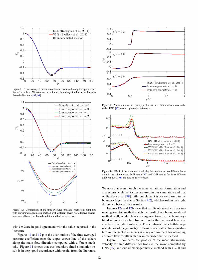
Figures 11 and 12 plot the distribution of the time-averagedpressure coefficient over the upper crown line of the spherealong the main flow direction computed with different meth-ods. Figure 11 shows that our boundary-fitted simulation re-sult is in very good accordance with results from the literature.
-0.4
0
0.4
0.8
1.2x/d = 0.2
u/U
-0.4
0
0.4
0.8
1.2x/d = 1.6
y/d0 0.5 1 1.5 2
-0.4
0
0.4
0.8
1.2x/d = 3.0
DNS (Rodriguez et al. 2011)Immersogeometric l = 0Immersogeometric l = 2
Figure 13: Mean streamwise velocity profiles at three different locations in thewake. DNS [97] result is plotted as reference.
0
0.1
0.2
x/d = 1.6
urm
s/U
y/d0 0.5 1 1.5 20
0.1
0.2
x/d = 3.0
DNS (Rodriguez et al. 2011)Immersogeometric l = 2VMS-W1 (Bazilevs et al. 2014)VMS-W2 (Bazilevs et al. 2014)VMS-W3 (Bazilevs et al. 2014)
Figure 14: RMS of the streamwise velocity fluctuations at two different loca-tions in the sphere wake. DNS result [97] and VMS results for three differenttime windows [98] are plotted as references.
We note that even though the same variational formulation andcharacteristic element sizes are used in our simulation and thatof Bazilevs et al. [98], different element types were used in theboundary layer mesh (see Section 4.2), which result in the slightdifference between our results.
Figures 12a and 12b show that results obtained with our im-mersogeometric method match the result of our boundary-fittedmethod well, while clear convergence towards the boundary-fitted reference can be observed under the increased levels ofadaptive quadrature sub-cells. This confirms that a faithful rep-resentation of the geometry in terms of accurate volume quadra-ture in intersected elements is a key requirement for obtainingaccurate flow results with our immersogeometric method.
Figure 13 compares the profiles of the mean streamwisevelocity at three different positions in the wake computed byDNS [97] and our immersogeometric method with l = 0 and
12
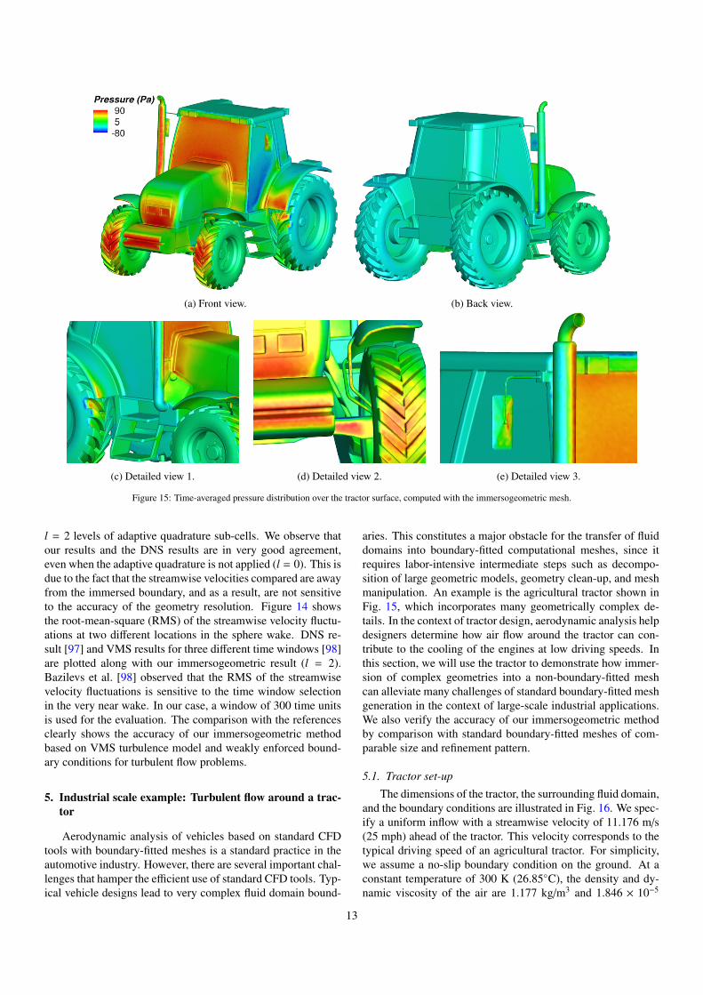
(a) Front view. (b) Back view.
(c) Detailed view 1. (d) Detailed view 2. (e) Detailed view 3.
Figure 15: Time-averaged pressure distribution over the tractor surface, computed with the immersogeometric mesh.
l = 2 levels of adaptive quadrature sub-cells. We observe thatour results and the DNS results are in very good agreement,even when the adaptive quadrature is not applied (l = 0). This isdue to the fact that the streamwise velocities compared are awayfrom the immersed boundary, and as a result, are not sensitiveto the accuracy of the geometry resolution. Figure 14 showsthe root-mean-square (RMS) of the streamwise velocity fluctu-ations at two different locations in the sphere wake. DNS re-sult [97] and VMS results for three different time windows [98]are plotted along with our immersogeometric result (l = 2).Bazilevs et al. [98] observed that the RMS of the streamwisevelocity fluctuations is sensitive to the time window selectionin the very near wake. In our case, a window of 300 time unitsis used for the evaluation. The comparison with the referencesclearly shows the accuracy of our immersogeometric methodbased on VMS turbulence model and weakly enforced bound-ary conditions for turbulent flow problems.
5. Industrial scale example: Turbulent flow around a trac-tor
Aerodynamic analysis of vehicles based on standard CFDtools with boundary-fitted meshes is a standard practice in theautomotive industry. However, there are several important chal-lenges that hamper the efficient use of standard CFD tools. Typ-ical vehicle designs lead to very complex fluid domain bound-
aries. This constitutes a major obstacle for the transfer of fluiddomains into boundary-fitted computational meshes, since itrequires labor-intensive intermediate steps such as decompo-sition of large geometric models, geometry clean-up, and meshmanipulation. An example is the agricultural tractor shown inFig. 15, which incorporates many geometrically complex de-tails. In the context of tractor design, aerodynamic analysis helpdesigners determine how air flow around the tractor can con-tribute to the cooling of the engines at low driving speeds. Inthis section, we will use the tractor to demonstrate how immer-sion of complex geometries into a non-boundary-fitted meshcan alleviate many challenges of standard boundary-fitted meshgeneration in the context of large-scale industrial applications.We also verify the accuracy of our immersogeometric methodby comparison with standard boundary-fitted meshes of com-parable size and refinement pattern.
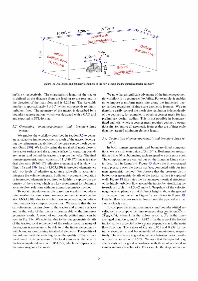
5.1. Tractor set-up
The dimensions of the tractor, the surrounding fluid domain,and the boundary conditions are illustrated in Fig. 16. We spec-ify a uniform inflow with a streamwise velocity of 11.176 m/s(25 mph) ahead of the tractor. This velocity corresponds to thetypical driving speed of an agricultural tractor. For simplicity,we assume a no-slip boundary condition on the ground. At aconstant temperature of 300 K (26.85C), the density and dy-namic viscosity of the air are 1.177 kg/m3 and 1.846 × 10⁻⁵
13
14 m 10.083 m 15.709 m
10 m
4.208 m
2.892 m
Inflow (uniform flow) 11.176 m/s
Outflow (traction free)
4.208 m
Lateral wall
(no penetration)
Ground
(no-slip wall)
Figure 16: Dimensions and boundary conditions of the flow domain and the immersed tractor geometry.
kg/(m·s), respectively. The characteristic length of the tractoris defined as the distance from the leading to the rear end inthe direction of the main flow and is 4.208 m. The Reynoldsnumber is approximately 3 × 10⁶, which corresponds to highlyturbulent flow. The geometry of the tractor is described by aboundary representation, which was designed with a CAD tooland exported in STL-format.
5.2. Generating immersogeometric and boundary-fittedmeshes
We employ the workflow described in Section 3.5 to gener-ate an adaptive immersogeometric mesh of the tractor, leverag-ing the refinement capabilities of the open-source mesh gener-ator Gmsh [90]. We locally refine the tetrahedral mesh close tothe tractor surface and the ground surface for capturing bound-ary layers, and behind the tractor to capture the wake. The finalimmersogeometric mesh consists of 11,489,570 linear tetrahe-dral elements (9,367,179 effective elements) and is shown inFigs. 17a and 17b. In all (1,953,920) intersected elements weadd two levels of adaptive quadrature sub-cells to accuratelyintegrate the volume integrals. Sufficiently accurate integrationin intersected elements is required to faithfully capture the ge-ometry of the tractor, which is a key requirement for obtainingaccurate flow solutions with our immersogeometric method.
To obtain simulation results based on standard boundary-fitted meshes for comparison, we use a commercial mesh gener-ator ANSA [108] due to its robustness in generating boundary-fitted meshes for complex geometries. We ensure that the lo-cal refinement pattern close to the tractor and ground surfacesand in the wake of the tractor is comparable to the immerso-geometric mesh. A zoom of our boundary-fitted mesh can beseen in Fig. 17c. We note that due to the fine geometric detailsof the tractor, local refinement of the surface mesh in many ofthe regions is necessary to be able to fit the fine-scale geometrywith boundary-conforming tetrahedral elements. The quality ofthe volume mesh depends highly on the quality of the surfacemesh used for its generation. The total number of elements inthe boundary-fitted mesh is 10,854,275, which is comparable tothe immersogeometric mesh.
We note that a significant advantage of the immersogeomet-ric workflow is its geometric flexibility. For example, it enablesus to impose a uniform mesh size along the immersed trac-tor surface regardless of fine-scale geometric features. We cantherefore easily control the mesh size resolution independentlyof the geometry, for example, to obtain a coarser mesh for fastpreliminary design studies. This is not possible in boundary-fitted analysis, where a coarser mesh requires geometry opera-tions first to remove all geometric features that are of finer scalethan the targeted minimum element length.
5.3. Comparison of immersogeometric and boundary-fitted re-sults
In both immersogeometric and boundary-fitted computa-tions, we use a time-step size of 3×10⁻⁴ s. Both meshes are par-titioned into 504 subdomains, each assigned to a processor core.The computations are carried out on the Lonestar Linux clus-ter described in Remark 4. Figure 15 shows the time-averagedstatic pressure over the tractor surface, computed with our im-mersogeometric method. We observe that the pressure distri-bution over geometric details of the tractor surface is capturedwell. Figure 18 illustrates the instantaneous vortical structuresof the highly turbulent flow around the tractor by visualizing theisosurfaces of λ2 = −1.5,−2 and −5. Snapshots of the velocitymagnitude on planar cuts at different heights above the groundat the same time instant as Figure 18 are shown in Figure 19.Detailed flow features such as flow around the pipe and mirrorscan be clearly seen.
To compare the immersogeometric and boundary-fitted re-sults, we first compute the time-averaged drag coefficient CD =
2FD/ρU2A, where U is the inflow velocity, FD is the time-averaged drag force, and A = 5.942 m2 is the area of the frontaltractor surface projected onto a plane perpendicular to the mainflow direction. The values of CD are 0.851 and 0.838 for theimmersogeometric and boundary-fitted computations, respec-tively. The results are in good agreement between the two meth-ods, with a deviation of 1.55%. We note that the reported dragcoefficients are in good accordance with those of observed insimilar industry benchmarks. For example, the drag coefficient
14
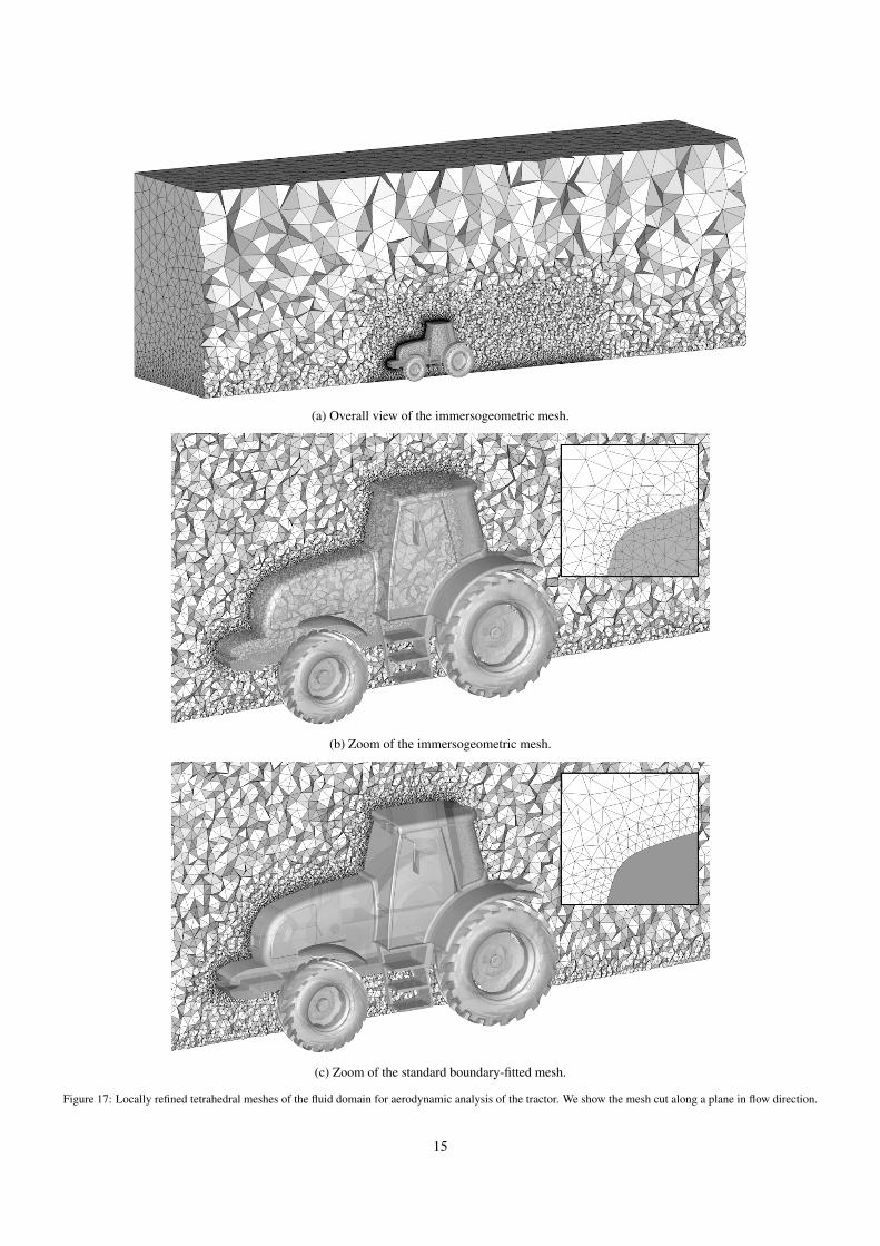
(a) Overall view of the immersogeometric mesh.
(b) Zoom of the immersogeometric mesh.
(c) Zoom of the standard boundary-fitted mesh.
Figure 17: Locally refined tetrahedral meshes of the fluid domain for aerodynamic analysis of the tractor. We show the mesh cut along a plane in flow direction.
15
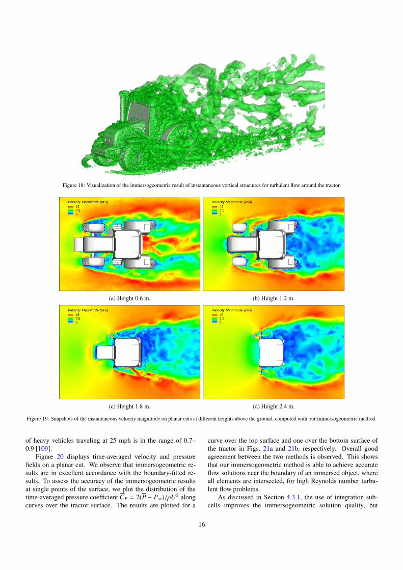
Figure 18: Visualization of the immersogeometric result of instantaneous vortical structures for turbulent flow around the tractor.
(a) Height 0.6 m. (b) Height 1.2 m.
(c) Height 1.8 m. (d) Height 2.4 m.
Figure 19: Snapshots of the instantaneous velocity magnitude on planar cuts at different heights above the ground, computed with our immersogeometric method.
of heavy vehicles traveling at 25 mph is in the range of 0.7–0.9 [109].
Figure 20 displays time-averaged velocity and pressurefields on a planar cut. We observe that immersogeometric re-sults are in excellent accordance with the boundary-fitted re-sults. To assess the accuracy of the immersogeometric resultsat single points of the surface, we plot the distribution of thetime-averaged pressure coefficient CP = 2(P − P∞)/ρU2 alongcurves over the tractor surface. The results are plotted for a
curve over the top surface and one over the bottom surface ofthe tractor in Figs. 21a and 21b, respectively. Overall goodagreement between the two methods is observed. This showsthat our immersogeometric method is able to achieve accurateflow solutions near the boundary of an immersed object, whereall elements are intersected, for high Reynolds number turbu-lent flow problems.
As discussed in Section 4.3.1, the use of integration sub-cells improves the immersogeometric solution quality, but
16
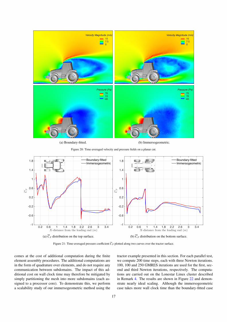
(a) Boundary-fitted. (b) Immersogeometric.
Figure 20: Time-averaged velocity and pressure fields on a planar cut.
X-distance from the leading end (m)0.2 0.6 1 1.4 1.8 2.2 2.6 3 3.4
CP
-1
-0.6
-0.2
0.2
0.6
1
1.4
1.8 Boundary-fittedImmersogeometric
(a) CP distribution on the top surface.
X-distance from the leading end (m)0.2 0.6 1 1.4 1.8 2.2 2.6 3 3.4
CP
-1
-0.6
-0.2
0.2
0.6
1
1.4
1.8 Boundary-fittedImmersogeometric
(b) CP distribution on the bottom surface.
Figure 21: Time-averaged pressure coefficient CP plotted along two curves over the tractor surface.
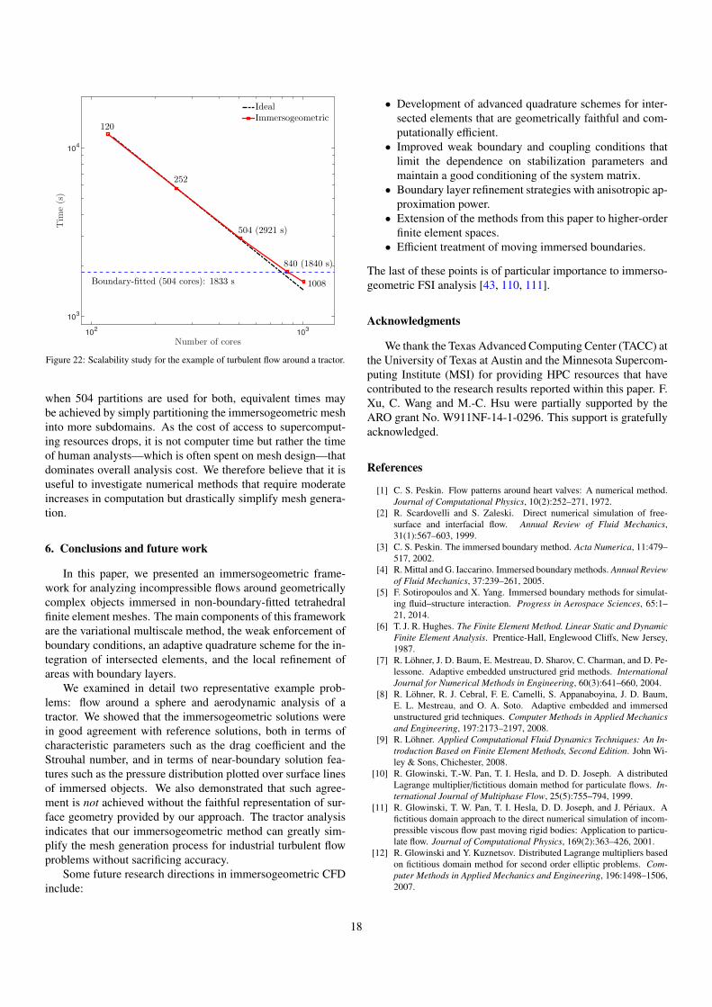
comes at the cost of additional computation during the finiteelement assembly procedures. The additional computations arein the form of quadrature over elements, and do not require anycommunication between subdomains. The impact of this ad-ditional cost on wall clock time may therefore be mitigated bysimply partitioning the mesh into more subdomains (each as-signed to a processor core). To demonstrate this, we performa scalability study of our immersogeometric method using the
tractor example presented in this section. For each parallel test,we compute 200 time steps, each with three Newton iterations.100, 100 and 250 GMRES iterations are used for the first, sec-ond and third Newton iterations, respectively. The computa-tions are carried out on the Lonestar Linux cluster describedin Remark 4. The results are shown in Figure 22 and demon-strate nearly ideal scaling. Although the immersogeometriccase takes more wall clock time than the boundary-fitted case
17
Number of cores102 103
Tim
e(s)
103
104
120
252
504 (2921 s)
840 (1840 s)
1008Boundary-fitted (504 cores): 1833 s
IdealImmersogeometric
Figure 22: Scalability study for the example of turbulent flow around a tractor.
when 504 partitions are used for both, equivalent times maybe achieved by simply partitioning the immersogeometric meshinto more subdomains. As the cost of access to supercomput-ing resources drops, it is not computer time but rather the timeof human analysts—which is often spent on mesh design—thatdominates overall analysis cost. We therefore believe that it isuseful to investigate numerical methods that require moderateincreases in computation but drastically simplify mesh genera-tion.
6. Conclusions and future work
In this paper, we presented an immersogeometric frame-work for analyzing incompressible flows around geometricallycomplex objects immersed in non-boundary-fitted tetrahedralfinite element meshes. The main components of this frameworkare the variational multiscale method, the weak enforcement ofboundary conditions, an adaptive quadrature scheme for the in-tegration of intersected elements, and the local refinement ofareas with boundary layers.
We examined in detail two representative example prob-lems: flow around a sphere and aerodynamic analysis of atractor. We showed that the immersogeometric solutions werein good agreement with reference solutions, both in terms ofcharacteristic parameters such as the drag coefficient and theStrouhal number, and in terms of near-boundary solution fea-tures such as the pressure distribution plotted over surface linesof immersed objects. We also demonstrated that such agree-ment is not achieved without the faithful representation of sur-face geometry provided by our approach. The tractor analysisindicates that our immersogeometric method can greatly sim-plify the mesh generation process for industrial turbulent flowproblems without sacrificing accuracy.
Some future research directions in immersogeometric CFDinclude:
• Development of advanced quadrature schemes for inter-sected elements that are geometrically faithful and com-putationally efficient.
• Improved weak boundary and coupling conditions thatlimit the dependence on stabilization parameters andmaintain a good conditioning of the system matrix.
• Boundary layer refinement strategies with anisotropic ap-proximation power.
• Extension of the methods from this paper to higher-orderfinite element spaces.
• Efficient treatment of moving immersed boundaries.
The last of these points is of particular importance to immerso-geometric FSI analysis [43, 110, 111].
Acknowledgments
We thank the Texas Advanced Computing Center (TACC) atthe University of Texas at Austin and the Minnesota Supercom-puting Institute (MSI) for providing HPC resources that havecontributed to the research results reported within this paper. F.Xu, C. Wang and M.-C. Hsu were partially supported by theARO grant No. W911NF-14-1-0296. This support is gratefullyacknowledged.
References
[1] C. S. Peskin. Flow patterns around heart valves: A numerical method.Journal of Computational Physics, 10(2):252–271, 1972.
[2] R. Scardovelli and S. Zaleski. Direct numerical simulation of free-surface and interfacial flow. Annual Review of Fluid Mechanics,31(1):567–603, 1999.
[3] C. S. Peskin. The immersed boundary method. Acta Numerica, 11:479–517, 2002.
[4] R. Mittal and G. Iaccarino. Immersed boundary methods. Annual Reviewof Fluid Mechanics, 37:239–261, 2005.
[5] F. Sotiropoulos and X. Yang. Immersed boundary methods for simulat-ing fluid–structure interaction. Progress in Aerospace Sciences, 65:1–21, 2014.
[6] T. J. R. Hughes. The Finite Element Method. Linear Static and DynamicFinite Element Analysis. Prentice-Hall, Englewood Cliffs, New Jersey,1987.
[7] R. Lohner, J. D. Baum, E. Mestreau, D. Sharov, C. Charman, and D. Pe-lessone. Adaptive embedded unstructured grid methods. InternationalJournal for Numerical Methods in Engineering, 60(3):641–660, 2004.
[8] R. Lohner, R. J. Cebral, F. E. Camelli, S. Appanaboyina, J. D. Baum,E. L. Mestreau, and O. A. Soto. Adaptive embedded and immersedunstructured grid techniques. Computer Methods in Applied Mechanicsand Engineering, 197:2173–2197, 2008.
[9] R. Lohner. Applied Computational Fluid Dynamics Techniques: An In-troduction Based on Finite Element Methods, Second Edition. John Wi-ley & Sons, Chichester, 2008.
[10] R. Glowinski, T.-W. Pan, T. I. Hesla, and D. D. Joseph. A distributedLagrange multiplier/fictitious domain method for particulate flows. In-ternational Journal of Multiphase Flow, 25(5):755–794, 1999.
[11] R. Glowinski, T. W. Pan, T. I. Hesla, D. D. Joseph, and J. Periaux. Afictitious domain approach to the direct numerical simulation of incom-pressible viscous flow past moving rigid bodies: Application to particu-late flow. Journal of Computational Physics, 169(2):363–426, 2001.
[12] R. Glowinski and Y. Kuznetsov. Distributed Lagrange multipliers basedon fictitious domain method for second order elliptic problems. Com-puter Methods in Applied Mechanics and Engineering, 196:1498–1506,2007.
18
[13] L. Zhang, A. Gerstenberger, X. Wang, and W. K. Liu. Immersed finiteelement method. Computer Methods in Applied Mechanics and Engi-neering, 193:2051–2067, 2004.
[14] W. K. Liu, D. W. Kim, and S. Tang. Mathematical foundations of theimmersed finite element method. Computational Mechanics, 39(3):211–222, 2007.
[15] X. S. Wang, L. T. Zhang, and W. K. Liu. On computational issues ofimmersed finite element methods. Journal of Computational Physics,228(7):2535–2551, 2009.
[16] X. Wang and L. T. Zhang. Modified immersed finite element method forfully-coupled fluid–structure interactions. Computer Methods in AppliedMechanics and Engineering, 267:150–169, 2013.
[17] H. Casquero, C. Bona-Casas, and H. Gomez. A NURBS-based im-mersed methodology for fluid–structure interaction. Computer Methodsin Applied Mechanics and Engineering, 284:943–970, 2015.
[18] F. P. T. Baaijens. A fictitious domain/mortar element method for fluid–structure interaction. International Journal for Numerical Methods inFluids, 35(7):743–761, 2001.
[19] L. Parussini. Fictitious domain approach via Lagrange multipliers withleast squares spectral element method. Journal of Scientific Computing,37(3):316–335, 2008.
[20] L. Parussini and V. Pediroda. Fictitious domain approach with hp-finiteelement approximation for incompressible fluid flow. Journal of Com-putational Physics, 228(10):3891–3910, 2009.
[21] A. Gerstenberger and W. A. Wall. Enhancement of fixed-grid methodstowards complex fluid–structure interaction applications. InternationalJournal for Numerical Methods in Fluids, 57:1227–1248, 2008.
[22] A. Gerstenberger and W. A. Wall. An embedded Dirichlet formulationfor 3D continua. International Journal for Numerical Methods in Engi-neering, 82:537–563, 2010.
[23] S. Shahmiri, A. Gerstenberger, and W. A. Wall. An XFEM-based em-bedding mesh technique for incompressible viscous flows. InternationalJournal for Numerical Methods in Fluids, 65:166–190, 2011.
[24] T. Ruberg and F. Cirak. Subdivision-stabilised immersed B-spline finiteelements for moving boundary flows. Computer Methods in AppliedMechanics and Engineering, 209–212:266–283, 2012.
[25] T. Ruberg and F. Cirak. A fixed-grid b-spline finite element technique forfluid–structure interaction. International Journal for Numerical Meth-ods in Fluids, 74(9):623–660, 2014.
[26] J. Baiges and R. Codina. The fixed-mesh ALE approach applied to solidmechanics and fluid–structure interaction problems. International Jour-nal for Numerical Methods in Engineering, 81:1529–1557, 2010.
[27] T. Wick. Fully Eulerian fluid–structure interaction for time-dependentproblems. Computer Methods in Applied Mechanics and Engineering,255:14–26, 2013.
[28] T. Richter and T. Wick. Finite elements for fluid–structure interactionin ALE and fully Eulerian coordinates. Computer Methods in AppliedMechanics and Engineering, 199:2633–2642, 2010.
[29] C. Hesch, A. J. Gil, A. Arranz Carreno, and J. Bonet. On continuumimmersed strategies for fluid–structure interaction. Computer Methodsin Applied Mechanics and Engineering, 247-248:51–64, 2012.
[30] T. Richter. A fully Eulerian formulation for fluid–structure-interactionproblems. Journal of Computational Physics, 233:227–240, 2013.
[31] T. J. R. Hughes, L. Mazzei, and K. E. Jansen. Large eddy simulationand the variational multiscale method. Computing and Visualization inScience, 3:47–59, 2000.
[32] T. J. R. Hughes, L. Mazzei, A. A. Oberai, and A. Wray. The multiscaleformulation of large eddy simulation: Decay of homogeneous isotropicturbulence. Physics of Fluids, 13:505–512, 2001.
[33] T. J. R. Hughes, G. Scovazzi, and L. P. Franca. Multiscale and stabilizedmethods. In E. Stein, R. de Borst, and T. J. R. Hughes, editors, Encyclo-pedia of Computational Mechanics, Volume 3: Fluids, chapter 2. JohnWiley & Sons, 2004.
[34] Y. Bazilevs, V. M. Calo, J. A. Cottrel, T. J. R. Hughes, A. Reali, andG. Scovazzi. Variational multiscale residual-based turbulence modelingfor large eddy simulation of incompressible flows. Computer Methodsin Applied Mechanics and Engineering, 197:173–201, 2007.
[35] Y. Bazilevs and T. J. R. Hughes. Weak imposition of Dirichlet boundaryconditions in fluid mechanics. Computers & Fluids, 36:12–26, 2007.
[36] Y. Bazilevs, C. Michler, V. M. Calo, and T. J. R. Hughes. Weak Dirichlet
boundary conditions for wall-bounded turbulent flows. Computer Meth-ods in Applied Mechanics and Engineering, 196:4853–4862, 2007.
[37] Y. Bazilevs, C. Michler, V. M. Calo, and T. J. R. Hughes. Isogeometricvariational multiscale modeling of wall-bounded turbulent flows withweakly enforced boundary conditions on unstretched meshes. ComputerMethods in Applied Mechanics and Engineering, 199:780–790, 2010.
[38] M.-C. Hsu, I. Akkerman, and Y. Bazilevs. Wind turbine aerodynamicsusing ALE–VMS: Validation and the role of weakly enforced boundaryconditions. Computational Mechanics, 50:499–511, 2012.
[39] A. Stavrev. The Role of Higher-Order Geometry Approximation andAccurate Quadrature in NURBS Based Immersed Boundary Methods.Master’s Thesis, Technische Universitat Munchen, 2012.
[40] L. Kudela. Highly Accurate Subcell Integration in the Context of TheFinite Cell Method. Master’s Thesis, Technische Universitat Munchen,2013.
[41] T. J. R. Hughes, J. A. Cottrell, and Y. Bazilevs. Isogeometric analysis:CAD, finite elements, NURBS, exact geometry, and mesh refinement.Computer Methods in Applied Mechanics and Engineering, 194:4135–4195, 2005.
[42] J. A. Cottrell, T. J. R. Hughes, and Y. Bazilevs. Isogeometric Analysis:Toward Integration of CAD and FEA. John Wiley & Sons, Chichester,2009.
[43] D. Kamensky, M.-C. Hsu, D. Schillinger, J. A. Evans, A. Aggarwal,Y. Bazilevs, M. S. Sacks, and T. J. R. Hughes. An immersogeometricvariational framework for fluid–structure interaction: Application to bio-prosthetic heart valves. Computer Methods in Applied Mechanics andEngineering, 284:1005–1053, 2015.
[44] J. Parvizian, A. Duster, and E. Rank. Finite cell method: h- and p- exten-sion for embedded domain methods in solid mechanics. ComputationalMechanics, 41:122–133, 2007.
[45] A. Duster, J. Parvizian, Z. Yang, and E. Rank. The finite cell method forthree-dimensional problems of solid mechanics. Computer Methods inApplied Mechanics and Engineering, 197:3768–3782, 2008.
[46] D. Schillinger and M. Ruess. The Finite Cell Method: A review inthe context of higher-order structural analysis of CAD and image-basedgeometric models. Archives of Computational Methods in Engineering,22(3):391–455, 2015.
[47] M. Ruess, D. Schillinger, Y. Bazilevs, V. Varduhn, and E. Rank. Weaklyenforced essential boundary conditions for NURBS-embedded andtrimmed NURBS geometries on the basis of the finite cell method. In-ternational Journal for Numerical Methods in Engineering, 95(10):811–846, 2013.
[48] M. Ruess, D. Schillinger, A. I. Ozcan, and E. Rank. Weak couplingfor isogeometric analysis of non-matching and trimmed multi-patch ge-ometries. Computer Methods in Applied Mechanics and Engineering,269:46–71, 2014.
[49] D. Schillinger and E. Rank. An unfitted hp adaptive finite elementmethod based on hierarchical B-splines for interface problems of com-plex geometry. Computer Methods in Applied Mechanics and Engineer-ing, 200(47–48):3358–3380, 2011.
[50] D. Schillinger, A. Duster, and E. Rank. The hp-d adaptive finite cellmethod for geometrically nonlinear problems of solid mechanics. Inter-national Journal for Numerical Methods in Engineering, 89:1171–1202,2012.
[51] D. Schillinger, L. Dede, M. A. Scott, J. A. Evans, M. J. Borden, E. Rank,and T. J. R. Hughes. An isogeometric design-through-analysis method-ology based on adaptive hierarchical refinement of NURBS, immersedboundary methods, and T-spline CAD surfaces. Computer Methods inApplied Mechanics and Engineering, 249-250:116–150, 2012.
[52] M. Joulaian and A. Duster. Local enrichment of the finite cell method forproblems with material interfaces. Computational Mechanics, 52:741–762, 2013.
[53] N. Zander, T. Bog, S. Kollmannsberger, D. Schillinger, and E. Rank.Multi-level hp-adaptivity: high-order mesh adaptivity without the dif-ficulties of constraining hanging nodes. Computational Mechanics,55:499–517, 2015.
[54] Z. Yang, M. Ruess, S. Kollmannsberger, A. Duster, and E. Rank. Anefficient integration technique for the voxel-based finite cell method. In-ternational Journal for Numerical Methods in Engineering, 91:457–471,2012.
19
[55] D. Schillinger, S. Kollmannsberger, R.-P. Mundani, and E. Rank. Thefinite cell method for geometrically nonlinear problems of solid me-chanics. IOP Conference Series: Material Science and Engineering,10:012170, 2010.
[56] D. Schillinger, M. Ruess, N. Zander, Y. Bazilevs, A. Duster, andE. Rank. Small and large deformation analysis with the p- and B-spline versions of the Finite Cell Method. Computational Mechanics,50(4):445–478, 2012.
[57] N. Zander, S. Kollmannsberger, M. Ruess, Z. Yosibash, and E. Rank.The Finite Cell Method for linear thermoelasticity. Computers & Math-ematics with Applications, 64(11):3527–3541, 2012.
[58] A. Duster, H.-G. Sehlhorst, and E. Rank. Numerical homogenizationof heterogeneous and cellular materials utilizing the finite cell method.Computational Mechanics, 50:413–431, 2012.
[59] M. Ruess, D. Tal, N. Trabelsi, Z. Yosibash, and E. Rank. The finite cellmethod for bone simulations: Verification and validation. Biomechanicsand Modeling in Mechanobiology, 11(3):425–437, 2012.
[60] J. Parvizian, A. Duster, and E. Rank. Topology optimization using thefinite cell method. Optimization and Engineering, 13:57–78, 2012.
[61] C. Willberg, S. Duczek, J. M. Vivar Perez, D. Schmicker, and U. Gab-bert. Comparison of different higher order finite element schemes forthe simulation of Lamb waves. Computer Methods in Applied Mechan-ics and Engineering, 241–244:246–261, 2012.
[62] S. Duczek, M. Joulaian, A. Duster, and U. Gabbert. Numerical analysisof Lamb waves using the finite and spectral cell methods. InternationalJournal for Numerical Methods in Engineering, 99(1):26–53, 2014.
[63] M. Joulaian, S. Duczek, U. Gabbert, and A. Duster. Finite and spectralcell method for wave propagation in heterogeneous materials. Compu-tational Mechanics, 54(1):661–675, 2014.
[64] N. Zander, T. Bog, M. Elhaddad, R. Espinoza, H. Hu, A. F. Joly,C. Wu, P. Zerbe, A. Dster, S. Kollmannsberger, J. Parvizian, M. Ruess,D. Schillinger, and E. Rank. FCMLab: A finite cell research toolbox forMATLAB. Advances in Engineering Software, 74:49–63,, 2014.
[65] V. Varduhn, M.-C. Hsu, M. Ruess, and D. Schillinger. The tetrahedralfinite cell method: Higher-order immersogeometric analysis on adap-tive non-boundary-fitted meshes. Submitted to International Journal forNumerical Methods in Engineering, 2015.
[66] A. N. Brooks and T. J. R. Hughes. Streamline upwind/Petrov-Galerkinformulations for convection dominated flows with particular emphasison the incompressible Navier–Stokes equations. Computer Methods inApplied Mechanics and Engineering, 32:199–259, 1982.
[67] T. E. Tezduyar. Stabilized finite element formulations for incompressibleflow computations. Advances in Applied Mechanics, 28:1–44, 1992.
[68] T. E. Tezduyar and Y. Osawa. Finite element stabilization parameterscomputed from element matrices and vectors. Computer Methods inApplied Mechanics and Engineering, 190:411–430, 2000.
[69] M.-C. Hsu, Y. Bazilevs, V. M. Calo, T. E. Tezduyar, and T. J. R. Hughes.Improving stability of stabilized and multiscale formulations in flowsimulations at small time steps. Computer Methods in Applied Mechan-ics and Engineering, 199:828–840, 2010.
[70] C. Johnson. Numerical Solution of Partial Differential Equations by theFinite Element Method. Cambridge University Press, Sweden, 1987.
[71] S. C. Brenner and L. R. Scott. The Mathematical Theory of Finite Ele-ment Methods, 2nd ed. Springer, Berlin, 2002.
[72] A. Ern and J. L. Guermond. Theory and Practice of Finite Elements.Springer, Berlin, 2004.
[73] J. Nitsche. Uber ein variationsprinzip zur losung von Dirichlet-problemen bei verwendung von teilraumen, die keinen randbedingungenunterworfen sind. Abh. Math. Univ. Hamburg, 36:9–15, 1971.
[74] A. Embar, J. Dolbow, and I. Harari. Imposing Dirichlet boundary con-ditions with Nitsche’s method and spline-based finite elements. Interna-tional Journal for Numerical Methods in Engineering, 83(7):877–898,2010.
[75] Y. Bazilevs and I. Akkerman. Large eddy simulation of turbulentTaylor–Couette flow using isogeometric analysis and the residual-basedvariational multiscale method. Journal of Computational Physics,229:3402–3414, 2010.
[76] N. Kikuchi. A smoothing technique for reduced integration penaltymethods in contact problems. International Journal for NumericalMethods in Engineering, 18(3):343–350, 1982.
[77] J. D. Sanders, J. E. Dolbow, and T. A. Laursen. On methods for sta-
bilizing constraints over enriched interfaces in elasticity. InternationalJournal for Numerical Methods in Engineering, 78:1009–1036, 2009.
[78] F. Liu and R. I. Borja. Stabilized low-order finite elements for frictionalcontact with the extended finite element method. Computer Methods inApplied Mechanics and Engineering, 199:2456–2471, 2010.
[79] L. De Lorenzis, I. Temizer, P. Wriggers, and G. Zavarise. A large defor-mation frictional contact formulation using NURBS-based isogeometricanalysis. International Journal for Numerical Methods in Engineering,87:1278–1300, 2011.
[80] R. A. Sauer and L. De Lorenzis. A computational contact formulationbased on surface potentials. Computer Methods in Applied Mechanicsand Engineering, 253(0):369–395, 2013.
[81] J. Chung and G. M. Hulbert. A time integration algorithm for struc-tural dynamics with improved numerical dissipation: The generalized-αmethod. Journal of Applied Mechanics, 60:371–75, 1993.
[82] K. E. Jansen, C. H. Whiting, and G. M. Hulbert. A generalized-αmethodfor integrating the filtered Navier-Stokes equations with a stabilized fi-nite element method. Computer Methods in Applied Mechanics and En-gineering, 190:305–319, 2000.
[83] Y. Bazilevs, V. M. Calo, T. J. R. Hughes, and Y. Zhang. Isogeometricfluid–structure interaction: theory, algorithms, and computations. Com-putational Mechanics, 43:3–37, 2008.
[84] Y. Saad and M. Schultz. GMRES: A generalized minimal residual algo-rithm for solving nonsymmetric linear systems. SIAM Journal of Scien-tific and Statistical Computing, 7:856–869, 1986.
[85] F. Shakib, T. J. R. Hughes, and Z. Johan. A multi-element group precon-ditioned GMRES algorithm for nonsymmetric systems arising in finiteelement analysis. Computer Methods in Applied Mechanics and Engi-neering, 75:415–456, 1989.
[86] C. Pozrikidis. Introduction to Finite and Spectral Element Methods Us-ing MATLAB, Second Edition. Taylor & Francis Group, Boca Raton,FL, 2014.
[87] I. Wald, W. R. Mark, J. Gunther, S. Boulos, T. Ize, W. Hunt, S. G.Parker, and P. Shirley. State of the art in ray tracing animated scenes.In Proceedings of the Annual Conference of the European Associationfor Computer Graphics, pages 89–116, 2007.
[88] J. Bigler, A. Stephens, and S. G. Parker. Design for parallel interactiveray tracing systems. In Proceedings of the IEEE Symposium on Interac-tive Ray Tracing 2006, pages 187–196, 2006.
[89] S. J. Owen. A survey of unstructured mesh generation technology. InProceedings of the 7th International Meshing Roundtable, pages 239–267, Sandia National Lab, 1998.
[90] C. Geuzaine and J.-F. Remacle. Gmsh: A 3-D finite element mesh gener-ator with built-in pre-and post-processing facilities. International Jour-nal for Numerical Methods in Engineering, 79(11):1309–1331, 2009.
[91] T. A. Johnson and V. C. Patel. Flow past a sphere up to a Reynoldsnumber of 300. Journal of Fluid Mechanics, 378:19–70, 1999.
[92] R. Mittal. A Fourier–Chebyshev spectral collocation method for simu-lating flow past spheres and spheroids. International journal for numer-ical methods in fluids, 30(7):921–937, 1999.
[93] S. Marella, S. Krishnan, H. Liu, and H. S. Udaykumar. Sharp inter-face Cartesian grid method I: An easily implemented technique for 3Dmoving boundary computations. Journal of Computational Physics,210(1):1–31, 2005.
[94] J.-I. Choi, R. C. Oberoi, J. R. Edwards, and J. A. Rosati. An immersedboundary method for complex incompressible flows. Journal of Com-putational Physics, 224(2):757–784, 2007.
[95] R. Mittal, H. Dong, M. Bozkurttas, F. M. Najjar, A. Vargas, and A. vonLoebbecke. A versatile sharp interface immersed boundary method forincompressible flows with complex boundaries. Journal of computa-tional physics, 227(10):4825–4852, 2008.
[96] G. Yun, D. Kim, and H. Choi. Vortical structures behind a sphere at sub-critical Reynolds numbers. Physics of Fluids, 18(1):015102–14, 2006.
[97] I. Rodriguez, R. Borell, O. Lehmkuhl, C. D. Perez Segarra, and A. Oliva.Direct numerical simulation of the flow over a sphere at Re = 3700.Journal of Fluid Mechanics, 679:263–287, 2011.
[98] Y. Bazilevs, J. Yan, M. de Stadler, and S. Sarkar. Computation of theflow over a sphere at Re = 3700: A comparison of uniform and turbulentinflow conditions. Journal of Applied Mechanics, 81(12):121003, 2014.
[99] E. H. van Brummelen, K. G. van der Zee, V. V. Garg, and S. Prudhomme.Flux evaluation in primal and dual boundary-coupled problems. Journalof Applied Mechanics, 79:010904, 2011.
20

[100] R. V. Garimella and M. S. Shephard. Boundary layer mesh generationfor viscous flow simulations. International Journal for Numerical Meth-ods in Engineering, 49(1-2):193–218, 2000.
[101] X. Li, M. S. Shephard, and M. W. Beall. 3D anisotropic mesh adaptationby mesh modification. Computer Methods in Applied Mechanics andEngineering, 194(48-49):4915–4950, 2005.
[102] Y. Zhang, W. Wang, X. Liang, Y. Bazilevs, M.-C. Hsu, T. Kvamsdal,R. Brekken, and J.G. Isaksen. High-fidelity tetrahedral mesh genera-tion from medical imaging data for fluid–structure interaction analysisof cerebral aneurysms. Computer Modeling in Engineering & Sciences,42:131–150, 2009.
[103] TACC Lonestar User Guide. https://portal.tacc.utexas.edu/user-guides/lonestar. 2015.
[104] Texas Advanced Computing Center (TACC). http://www.tacc.utexas.edu. 2015.
[105] M.-C. Hsu, I. Akkerman, and Y. Bazilevs. High-performance computingof wind turbine aerodynamics using isogeometric analysis. Computers& Fluids, 49:93–100, 2011.
[106] G. Karypis and V. Kumar. A fast and high quality multilevel scheme for
partitioning irregular graphs. SIAM Journal on Scientific Computing,20:359–392, 1999.
[107] J. Jeong and F. Hussain. On the identification of a vortex. Journal ofFluid Mechanics, 285:69–94, 1995.
[108] BETA CAE Systems S.A. – ANSA pre-processor. http://www.beta-cae.gr/ansa.htm. 2015.
[109] V. Malviya, R. Mishra, and J. D. Fieldhouse. CFD investigation of anovel fuel-saving device for articulated tractor-trailer combinations. En-gineering Applications of Computational Fluid Mechanics, 3(4):587–607, 2009.
[110] M.-C. Hsu, D. Kamensky, Y. Bazilevs, M. S. Sacks, and T. J. R.Hughes. Fluid–structure interaction analysis of bioprosthetic heartvalves: significance of arterial wall deformation. Computational Me-chanics, 54(4):1055–1071, 2014.
[111] M.-C. Hsu, D. Kamensky, F. Xu, J. Kiendl, C. Wang, M. C. H. Wu,J. Mineroff, A. Reali, Y. Bazilevs, and M. S. Sacks. Dynamic and fluid–structure interaction simulations of bioprosthetic heart valves using para-metric design with T-splines and Fung-type material models. Computa-tional Mechanics, 55:1211–1225, 2015.
21