· the transformation between the covariant and contra-variant components for the metric tensor...
TRANSCRIPT

ERROR ANALYSIS OF THE GENERALIZED MAC SCHEME
YIN-LIANG HUANG∗, JIAN-GUO LIU† , AND WEI-CHENG WANG‡
Abstract.
We present a rigorous convergence analysis for the generalized MAC (GMAC) scheme on curvilinear domains proposedearlier by the authors [HLW]. The error estimate for the velocity field is established by energy estimate utilizing the streamfunction and discrete identities associated with the spatially compatible discretization. The spatially compatible discretizationalso induces subtle stabilizing effect that renders the scheme uniform LBB bound even though GMAC is staggered and supportedthe same way as the Q1 − P0 finite element method, which is well known to be unstable under divergence constraint. As aresult, full second order error estimate is achieved for both velocity and pressure with minimal regularity requirement.
1. Introduction. A generalized MAC scheme (GMAC) for the Navier-Stokes equation in rotationalform
(1.1)ut + ω × u + ∇p = ν∇2u + f on Ω
∇ · u = 0 on Ωu = 0 on Γ
on curvilinear domains was introduced in [HLW]. With partially staggered grids (velocity componentscollocated on cell centers, pressure placed on grid points) and centered difference in a locally ’skewed’coordinate, the discretization preserves crucial identities such as
(1.2) curlh gradh ≡ 0, divh curlh ≡ 0
and their converse in the discrete setting. The resulting scheme is simple and efficient with full second orderaccuracy on curvilinear domains. A key ingredient of the scheme is the proper treatment at the boundary,which not only enforces the pressure as discrete Lagrangian multiplier without introduction artificial bound-ary conditions, but also leads to an exact Hodge decomposition for the velocity field, which plays a key rolein both stability and efficiency of the scheme.
In this paper, we will show that the spatial compatibility (1.2) (recast as Lemma 2.1 in section 2) alsoleads to a simple error estimate for the velocity field. Optimal error analysis for the classical MAC schemewas first obtained in [HW], and in [W1] for MAC-like schemes on Cartesian grids. The proof in [HW, W1]is based on high order Strang’s expansion. Here we present an alternative approach that relies mainly onthe special structure of the spatial discretization, making use of both the stream function and the discretedifferential identities in Lemma 2.1. As a result, we obtain optimal O(h2) error estimate for the velocityfield provided the exact solution satisfies ue ∈ L2(0, T ;C4(Ω)) ∩H1(0, T ;C2(Ω)) and pe ∈ L2(0, T ;C3(Ω))(Theorem 1, section 3.1). This may be the minimal regularity requirement in finite difference setting.
On the other hand, the error analysis for the pressure is much more subtle due to lack of evolutionaryequation. Our approach is based on establishing the Ladyzhenskaya-Babuska-Brezzi condition (also knownas the LBB, div-stability or inf-sup condition) for the generalized MAC scheme. The LBB condition providesdirect access to pressure error estimate for the dynamic problem (1.1), and is essential to the solvability anduniform estimate for the static Stokes problem. It is worth noting that GMAC is staggered the same way asthe Q1−P0 finite element method, which is known to violate the uniform LBB condition. The main differencebetween the two schemes is the discretization of the viscous term. The spatially compatible discretizationassociated with GMAC induces subtle stabilizing effect and is key to the uniform LBB bound. As a result, we
∗Department of Applied Mathematics, National University of Tainan, Tainan, 700, Taiwan. ([email protected])†Department of Physics and Department of Mathematics, Duke University, Durham, NC 27708, USA
([email protected])‡Department of Mathematics, National Tsing Hua University, HsinChu, 300, Taiwan. ([email protected])
1
×
ξ2= constant
×
ξ2= constant
ξ2= constant
ξ2= constant
×
ξ1= constant
×
ξ1= constant
ξ1= constantξ1
= constant
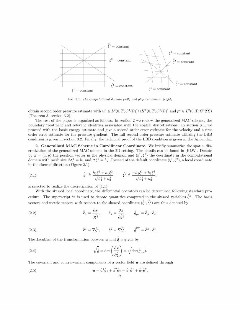
Fig. 2.1. The computational domain (left) and physical domain (right)
obtain second order pressure estimate with ue ∈ L2(0, T ;C4(Ω))∩H1(0, T ;C3(Ω)) and pe ∈ L2(0, T ;C3(Ω))(Theorem 3, section 3.2).
The rest of the paper is organized as follows. In section 2 we review the generalized MAC scheme, theboundary treatment and relevant identities associated with the spatial discretizations. In section 3.1, weproceed with the basic energy estimate and give a second order error estimate for the velocity and a firstorder error estimate for the pressure gradient. The full second order pressure estimate utilizing the LBBcondition is given in section 3.2. Finally, the technical proof of the LBB condition is given in the Appendix.
2. Generalized MAC Scheme in Curvilinear Coordinate. We briefly summarize the spatial dis-cretization of the generalized MAC scheme in the 2D setting. The details can be found in [HLW]. Denoteby x = (x, y) the position vector in the physical domain and (ξ1, ξ2) the coordinate in the computationaldomain with mesh size ∆ξ1 = h1 and ∆ξ2 = h2. Instead of the default coordinate (ξ1, ξ2), a local coordinatein the skewed direction (Figure 2.1)
(2.1)×
ξ1 ,h2ξ
1 + h1ξ2
√
h21 + h2
2
,×
ξ2 ,−h2ξ
1 + h1ξ2
√
h21 + h2
2
.
is selected to realize the discretization of (1.1).With the skewed local coordinate, the differential operators can be determined following standard pro-
cedure. The superscript ‘×’ is used to denote quantities computed in the skewed variables×
ξα. The basis
vectors and metric tensors with respect to the skewed coordinate (×
ξ1,×
ξ2) are thus denoted by
(2.2)×
e1 =∂x
∂×
ξ1,
×
e2 =∂x
∂×
ξ2,
×
gµν =×
eµ · ×
eν ,
(2.3)×
e1 = ∇×
ξ1,×
e2 = ∇×
ξ2,×
gµν
=×
eµ · ×
eν .
The Jacobian of the transformation between x and×
ξ is given by
(2.4)
√
×
g = det
(
∂x
∂×
ξ
)
=√
det(×
gµν).
The covariant and contra-variant components of a vector field u are defined through
(2.5) u =×
u1×
e1 +×
u2×
e2 =×
u1×
e1 +×
u2×
e2.
2

The transformation between the covariant and contra-variant components for the metric tensor and for avector field are given by
(2.6)
2∑
γ=1
×
gµγ×
gγν = δµν
and
(2.7)×
uµ =
2∑
γ=1
×
gµγ ×
uγ ,×
uν =
2∑
γ=1
×
gγν×
uγ , µ, ν = 1, 2.
The discretization of (1.1) is based on centered difference approximation of the intrinsic differentialoperators given below in (2.19)-(2.23). The metric tensors involved there can be calculated either analytically,given explicit form of the mapping (ξ1, ξ2) 7→ (x, y), or numerically from centered difference approximationof (2.2) for the covariant component, and then from (2.4) and (2.6) for the numerical Jacobian and contra-variant components.
Here for simplicity of presentation, we assume the physical domain Ω is diffeomorphic to a ring, sothat a single coordinate chart (ξ1, ξ2) ∈ (0, 1) × S1 is sufficient to represent the computational domain.The generalized MAC scheme can be applied to a generic domain by decomposing it into non-overlappingquadrilateral sub-domains. The details of the discretizations on coordinate interfaces and junctions, as wellas the 3D case can be found in [HLW].
We further assume equal spacing in ξ1 and ξ2:
(2.8) h1 = h2 = h =
×
h√2
=1
N,
where×
h = ∆×
ξ1 = ∆×
ξ2 = 2h1h2√h21+h2
2
is the natural grid spacing in the skewed variables. When h1 = h2, we also
have√g =
√
×
g. The relevant domains for spatial discretizations are summarized as follows:
Ωc ,
x(ξ1i− 12
, ξ2j− 12
) | 1 ≤ i ≤ N ; 1 ≤ j ≤ N
(2.9)
Ωg ,
x(ξ1i , ξ2j ) | 1 ≤ i ≤ N − 1; 1 ≤ j ≤ N
(2.10)
Ωg ,
x(ξ1i , ξ2j ) | 0 ≤ i ≤ N ; 1 ≤ j ≤ N
(2.11)
Γg , Ωg \ Ωg(2.12)
Ωge,
x(ξ1i , ξ2j ) ∈ Ωg | i+ j is even
(2.13)
Ωgo,
x(ξ1i , ξ2j ) ∈ Ωg | i+ j is odd
(2.14)
By assumption, all scalar and vector fields under consideration, including
L2(Ωg,R) ,
ω : Ωg → R
(2.15)
L2(Ωc,R2) ,
u : Ωc → R2
(2.16)
and
L2(Ωg,R)/R2 ,
p ∈ L2(Ωg,R)∣
∣
∑
Ωge
′(
√
×
ghp)i,j = 0 =∑
Ωgo
′(
√
×
ghp)i,j
,(2.17)
L2c(Ωg,R) ,
ψ ∈ L2(Ωg,R)∣
∣ψi,j = constant on i = 0 and i = N, respectively
(2.18)
3

are all periodic in ξ2. Here in (2.17), the primed sums denote summing with half weight on boundary gridsΓg ∩ Ωge
and Γg ∩ Ωgorespectively.
For ω, p ∈ L2(Ωg,R) and u =×
u1×
e1 +×
u2×
e2 =×
u1×
e1 +×
u2×
e2 ∈ L2(Ωc,R2), we define
(2.19)×
∇h : L2(Ωg,R) 7→ L2(Ωc,R2),
×
∇hp , (×
D1p)×
e1 + (×
D2p)×
e2
(2.20)×
∇⊥h : L2(Ωg,R) 7→ L2(Ωc,R
2),×
∇⊥h ω ,
−×
D2ω√
×
gh
×
e1 +
×
D1ω√
×
gh
×
e2
(2.21)×
∇′h· : L2(Ωc,R
2) 7→ L2(Ωg,R),×
∇′h · u =
1√
×
gh
(×
D′1(
√
×
gh×
u1) +×
D′2(
√
×
gh×
u2))
(2.22)×
∇⊥′h · : L2(Ωc,R
2) 7→ L2(Ωg,R),×
∇⊥′h · u =
1√
×
gh
(×
D′1×
u2 −×
D′2×
u1)
and
(2.23)×
′h : L2(Ωg,R) 7→ L2(Ωg,R),
×
′hp =
1√
×
gh
2∑
µ,ν=1
×
D′µ(
√
×
gh×
gµν
h
×
Dνp).
The primed operators in (2.21)-(2.23) denote the ‘reduced’ operators following Anderson [AN]. Thereduction only takes place near boundary, where all quantities involving the metric tensors located outsidethe computational domain are set to zero, followed by proper normalization. For example, at interior grids1 < i < N , (2.23) gives the full Laplacian
(×
′hp)i,j = (
×
hp)i,j =1
√
×
ghi,j
(×
q11h
×
D1p+×
q12h
×
D2p)i+ 12,j+ 1
2
×
h+
(×
q21h
×
D1p+×
q22h
×
D2p)i− 12,j+ 1
2
×
h
−(×
q11h
×
D1p+×
q12h
×
D2p)i− 12
,j− 12
×
h−
(×
q21h
×
D1p+×
q22h
×
D2p)i+ 12,j− 1
2
×
h
(2.24)
where×
qαβh =
√
×
gh×
gαβ
h . At a boundary grid, say i = 0, the discrete Laplacian reduces to
(2.25) (×
′hp)0,j =
2√
×
gh0,j
(×
q11h
×
D1p+×
q12h
×
D2p) 12,j+ 1
2
×
h−
(×
q21h
×
D1p+×
q22h
×
D2p) 12,j− 1
2
×
h
.
The detailed formula of (2.19)-(2.23) can be found in [HLW]. It can be shown that
(2.26) ker(×
′h) = ker(
×
∇h) = span1Ωge,1Ωgo
In case N is odd, Ωgeand Ωgo
coincide due to periodicity in ξ2. To be definite, we assume without loss of
generality that N is even and therefore dim(
ker(×
′h))
= dim(
ker(×
∇h))
= 2.
4

The significance of the reduced operator can be seen from the role it plays in the adjointness with respectto the natural inner products:
〈u , v 〉Ωc= h2
N∑
i=1
N∑
j=1
(
(u · v)√gh
)
i− 12,j− 1
2
= h2N∑
i=1
N∑
j=1
(
(×
u1×
v1 +×
u2×
v2)√gh
)
i− 12
,j− 12
= h2N∑
i=1
N∑
j=1
(
(×
u1×
v1 +×
u2×
v2)√gh
)
i− 12,j− 1
2
, u, v ∈ L2(Ωc,R2),
(2.27)
(2.28) 〈 a , b 〉Ωg= h2
M∑
i=0
′N∑
j=1
(
a b√gh
)
i,j, a, b ∈ L2(Ωg,R).
More precisely, we have the following Lemma from [HLW] which plays an essential role in the error analysisto be presented below:
Lemma 2.1. Let u ∈ L2(Ωc,R2) and a ∈ L2(Ωg,R), we have
1.
(2.29) 〈u ,×
∇ha 〉Ωc= −〈
×
∇′h · u , a 〉Ωg
2.
(2.30) 〈u ,×
∇⊥h a 〉Ωc
= −〈×
∇⊥′h · u , a 〉Ωg
3.
(2.31)×
∇′h ·
×
∇ha =×
∇⊥′h ·
×
∇⊥h a =
×
′ha on Ωg;
4. If a ∈ L2(Ωg,R), then
(2.32)×
∇′h ·
×
∇⊥h a =
×
∇⊥′h ·
×
∇ha = 0 on Ωg.
In addition, if a ∈ L2c(Ωg,R), then
(2.33)×
∇′h ·
×
∇⊥h a =
×
∇⊥′h ·
×
∇ha = 0 on Ωg.
In addition to Lemma 2.1, the reduced operators also provide a way of incorporating the no-slip, no-penetration conditions at the physical boundary. The resulting scheme for (1.1) is given by
(2.34)
ut + ωu⊥ +×
∇hp = ν×
∇⊥h ω + f on Ωc
ω =×
∇⊥′h · u on Ωg
×
∇′h · u = 0 on Ωg
The reduced divergence operator in the third equation of (2.34) has implicitly incorporated the no-penetrationcondition u · n = 0 in a natural way. On the other hand, the reduced curl operator in the second equationof (2.34) has implicitly incorporated the no-slip condition u × n = 0 on Γg. This can be interpreted as animplicit form of local vorticity boundary condition.
5

3. Error Estimate for the Generalized MAC Scheme. We now proceed with our main result,the second order error estimate for the generalized MAC scheme. Rigorous 2nd order error estimate forthe classical MAC scheme and some variants were first obtained in [HW] and [W1]. The method used in[HW, W1] is a combination of energy estimate and high order Strang’s expansion. Here we propose analternative proof and apply it to our scheme. In addition to extending the analysis to curvilinear domains,our method differs from [HW, W1] in several aspects. The first new component in our analysis is to utilize thestream function and combine it with the discrete identity (2.33) in our analysis. As a result, the regularityrequirement on the exact solution becomes transparent and less stringent. Secondly, our pressure erroranalysis is established via uniform inf-sup (LBB) estimate, which is of independent importance and haspotential applications in other areas such as computational elasticity and computational electromagnetics.The verification of the inf-sup condition is quite technical and is left in the Appendix.
3.1. Basic Error Estimate. Our first main result, 2nd order error estimate for the velocity field, isobtained from basic energy estimate.
Theorem 1. Assume the mapping x : (ξ1, ξ2) 7→ (x, y) is a C4 bijection from [0, 1]×S1 to Ω ⊂ R2. Let
ue ∈ L2(0, T ;C4(Ω)) ∩H1(0, T ;C2(Ω)), pe ∈ L2(0, T ;C3(Ω)) be an exact solution of (1.1), and uh, ωh, ph
the numerical solution of (2.34) with initial velocity uh0 satisfying
×
∇′h · uh
0 = 0. Then we have
max[0,T ]
‖uh − ue‖2Ωc
+ ν
∫ T
0
‖ωh − ωe‖2Ωg
≤ K1(‖uh0 − ue
0‖2Ωc
+×
h4),(3.1)
∫ T
0
‖×
∇h(ph − pe)‖2Ωc
≤ K2
(×
h−2‖uh0 − ue
0‖2Ωc
+×
h2)
.(3.2)
where K1, K2 are constants depending on T , ν, ‖ue‖L2(0,T ;C4(Ω)), ‖ue‖H1(0,T ;C2(Ω)), ‖pe‖L2(0,T ;C3(Ω)), but
not on×
h.A crucial part of Theorem 1 is to utilize the exact stream function ψe to construct a divergence free
approximate solution of the form
(3.3) ua(t, ·) =×
∇⊥h (ψe +
×
h2ϕ) ∈ L2(Ωc,R2)
such that both ua − ue and uh − ua are O(h2). The latter requires in addition that×
∇⊥′h · ua − ωe =
×
′h(ψe +
×
h2ϕ) − ωe = O(h2). Here ϕ is a correction to be determined from the following Lemma.Lemma 3.1. If the mapping x : (ξ1, ξ2) 7→ (x, y) is a C4 bijection from [0, 1] × S1 to Ω ⊂ R
2 andψ ∈ C4(Ω), then
×
′hψ(
x(0, ξ2))
=(2
√2
×
h
(
g11∂1ψ + g12∂2ψ)
+ ψ)
(
x(0, ξ2))
+ PL(ψ)(ξ2)×
h+QhL(ψ)(ξ2)
×
h2,
×
′hψ(
x(1, ξ2))
=(−2
√2
×
h
(
g11∂1ψ + g12∂2ψ)
+ ψ)
(
x(1, ξ2))
+ PR(ψ)(ξ2)×
h+QhR(ψ)(ξ2)
×
h2,
(3.4)
where
(3.5) ‖PL,R(ψ)‖C1(S1) + ‖QhL,R(ψ)‖C0(S1) ≤ C
[
‖x‖C4([0,1]×S1), ‖x−1‖C4(Ω)
]
‖ψ‖C4(Ω).
Here in (3.5) and the rest of the paper, we denote by C[
· · ·]
a positive constant that depends on thearguments inside the bracket.
Proof. We apply the reduced Laplacian (2.25) to ψ on x(0, ξ2) and split it into two parts:
(3.6)×
′hψ(
x(0, ξ2))
=2
√
×
g(0, ξ2)
(
IL,+(0, ξ2) + IL,−(0, ξ2))
6

where IL,±(0, ξ2) are the terms associated with×
qαβ(h2 , ξ
2 ± h2 ) =
√
×
g×
gαβ(h2 , ξ
2 ± h2 ), respectively. More
precisely,
IL,+(0, ξ2) ,1×
h
(
×
q11×
D1ψ +×
q12×
D2ψ)
(h2 , ξ
2 + h2 )
=1×
h
×
q11(h2 , ξ
2 + h2 )(×
∂1ψ(h2 , ξ
2 + h2 ) +
×
h2
24
×
∂31 ψ(h
2 , ξ2 + h
2 ) +KhL,1,+(ψ)(ξ2)
×
h3)
+1×
h
×
q12(h2 , ξ
2 + h2 )(×
∂2ψ(h2 , ξ
2 + h2 ) +
×
h2
24
×
∂32ψ(h
2 , ξ2 + h
2 ) +KhL,2,+(ψ)(ξ2)
×
h3)
(3.7)
where ψ = ψx and the remainder terms satisfy |KhL,ℓ,+(ψ)(ξ2)| ≤ C
[
‖x‖C4([0,1]×S1)
]
‖ψ‖C4(Ω), and we haveassumed that analytic metric tensors have been adopted in the discretization. The analysis below applies tonumerical metric tensors without difficulty.
Expand (3.7) around (0, ξ2) and apply (2.2), we get
IL,+(0, ξ2) =1×
h
(×
q11×
∂1ψ +×
q12×
∂2ψ)
(0, ξ2) +1
2
×
∂1
(×
q11×
∂1ψ +×
q12×
∂2ψ)
(0, ξ2)
+ PL,+(ψ)(ξ2)×
h+ QhL,+(ψ)(ξ2)
×
h2
(3.8)
where |QhL,+(ψ)(ξ2)| ≤ C
[
‖x‖C4([0,1]×S1), ‖x−1‖C4(Ω)
]
‖ψ‖C4(Ω) and
(3.9) PL,+(ψ)(ξ2) ,1
8
×
∂21
(×
q11×
∂1ψ +×
q12×
∂2ψ)
(0, ξ2) +1
24
(×
q11×
∂31 ψ +
×
q12×
∂32 ψ)
(0, ξ2).
Similarly,
IL,−(0, ξ2) ,−1×
h
(
×
q21×
D1ψ +×
q22×
D2ψ)
(h2 , ξ
2 − h2 )
= − 1×
h
(×
q21×
∂1ψ +×
q22×
∂2ψ)
(0, ξ2) +1
2
×
∂2
(×
q21×
∂1ψ +×
q22×
∂2ψ)
(0, ξ2)
− PL,−(ψ)(ξ2)×
h+ QhL,−(ψ)(ξ2)
×
h2
(3.10)
where |QhL,−(ψ)(ξ2)| ≤ C
[
‖x‖C4([0,1]×S1), ‖x−1‖C4(Ω)
]
‖ψ‖C4(Ω) and
(3.11) PL,−(ψ)(ξ2) ,1
8
×
∂22
(×
q21×
∂1ψ +×
q22×
∂2ψ)
(0, ξ2) +1
24
(×
q21×
∂31 ψ +
×
q22×
∂32 ψ)
(0, ξ2).
From (2.1), (2.8) and the relation
(3.12)×
g11 − 2
×
g21
+×
g22
= 2g11,×
g11 − ×
g22
= 2g12,
we have
(3.13)1×
h
(
×
q11×
∂1ψ +×
q12×
∂2ψ − ×
q21×
∂1ψ − ×
q22×
∂2ψ)
=
√2
√
×
g×
h
(
g11∂1ψ + g12∂2ψ)
.
7

As a consequence, (3.4) follows from (3.6), (3.8) and (3.10) with
PL(ψ)(ξ2) ,2
√
×
g(0, ξ2)
(
PL,+(ψ)(ξ2) − PL,−(ψ)(ξ2))
,
QhL(ψ)(ξ2) ,
2√
×
g(0, ξ2)
(
QhL,+(ψ)(ξ2) + Qh
L,−(ψ)(ξ2))
.
The estimate for PR and QhR are similar.
From Lemma 3.1, it is clear that |ωe(t, ·) − ωa(t, ·)| = O(h2) provided ϕ satisfies
ϕ(
t,x(0, ξ2))
= 0, ∂ξ1ϕ(
t,x(0, ξ2))
=−PL(ψe)(t, ξ2)
2√
2g11(0, ξ2),
ϕ(
t,x(1, ξ2))
= 0, ∂ξ1ϕ(
t,x(1, ξ2))
=PR(ψe)(t, ξ2)
2√
2g11(1, ξ2).
(3.14)
with PL,R(ψe) obtained by applying Lemma 3.1 to the exact stream function ψe(t, ·).Such a correction ϕ could be constructed by combining direct tensor products of fL,R with proper cutoff
functions in ξ1. However, for regularity consideration, we will elaborate further by mollifying fL and fR inthe ξ2 direction, with support of the mollifier proportional to the distance to Γ. The singularity inducedby vanishing support of the mollifier near the boundary can be compensated by the condition ϕ = 0 on Γ.More precisely, we have the following Lemma:
Lemma 3.2. Given fL and fR ∈ C1(S1), there exists a function ϕ ∈ C2([0, 1] × S1) such that
(3.15) ϕ(0, ξ2) = 0, ϕ(1, ξ2) = 0,
(3.16) ∂1ϕ(0, ξ2) = fL(ξ2), ∂1ϕ(1, ξ2) = fR(ξ2),
and
(3.17) ‖ϕ‖C2([0,1]×S1) ≤ C(
‖fL‖C1(S1) + ‖fR‖C1(S1)
)
.
Proof. Let η(·) : S1 7→ R be a standard mollifier with compact support [−δ, δ] ⊂ S1 and total mass 1,
∫
S1
η(ξ2) dξ2 = 1, ηǫ(ξ2) ,1
ǫη(ξ2
ǫ).
We define
ϕL(ξ1, ξ2) = ξ1(
ηξ1 ∗ fL
)
(ξ2) =
∫
S1
η(ξ2 − λ
ξ1)fL(λ) dλ,(3.18)
ϕR(ξ1, ξ2) =(1 − ξ1)(
η1−ξ1 ∗ fR
)
(ξ2) =
∫
S1
η(ξ2 − λ
1 − ξ1)fR(λ) dλ,(3.19)
and
(3.20) ϕ(ξ1, ξ2) = ϕL(ξ1, ξ2)Θ(ξ1) − ϕR(ξ1, ξ2)Θ(1 − ξ1),
8

where Θ is a smooth cutoff function satisfying
(3.21) Θ(ξ1) =
1, 0 ≤ ξ1 ≤ 13
0, 23 ≤ ξ1 ≤ 1
smoothly connected on 13 ≤ ξ1 ≤ 2
3
It is easy to see that ϕ satisfies (3.15). To show that ϕ satisfies (3.16), we note that
∂ξ1(ξ1ηξ1
(ξ2)) =∂ξ1η(ξ2
ξ1)
=−ξ2(ξ1)2
η′(ξ2
ξ1)
=1
ξ1ζ(ξ2
ξ1)
= ζξ1
(ξ2),(3.22)
where ζ(ξ2) , −ξ2η′(ξ2), is another mollifier with total mass 1 and ζǫ(ξ2) , 1ǫ ζ(
ξ2
ǫ ). Therefore
limξ1→0+
∂ξ1 ϕL(ξ1, ξ2) = limξ1→0+
∫
S1
∂ξ1(ξ1ηξ1
)(ξ2 − λ)fL(λ) dλ = limξ1→0+
∫
S1
ζξ1
(ξ2 − λ)fL(λ) dλ = fL(ξ2).
(3.23)
Similarly,
(3.24) limξ1→1−
∂ξ1 ϕR(ξ1, ξ2) = −fR(ξ2).
To estimate the C2-norm of ϕ(ξ1, ξ2), we first observe that
∣
∣∂2ξ2 ϕL(ξ1, ξ2)
∣
∣ =∣
∣
∫
S1
∂2ξ2 η(
ξ2 − λ
ξ1)fL(λ) dλ
∣
∣ =∣
∣
∫
S1
∂λ∂ξ2 η(ξ2 − λ
ξ1)fL(λ) dλ
∣
∣
=∣
∣
∫
S1
∂ξ2 η(ξ2 − λ
ξ1)∂λfL(λ) dλ
∣
∣ ≤ ‖fL‖C1(S1)‖η′‖L1(S1).
(3.25)
Secondly
∂ξ1ζξ1
(ξ2 − λ) = ∂ξ1
( 1
ξ1ζ(ξ2 − λ
ξ1))
=−1
ξ1( 1
ξ1ζ(ξ2 − λ
ξ1) +
ξ2 − λ
(ξ1)2ζ′(ξ2 − λ
ξ1))
=1
ξ1∂λ
(ξ2 − λ
ξ1ζ(ξ2 − λ
ξ1))
= ∂λZξ1
(ξ2 − λ)
(3.26)
where
(3.27) Z(ξ2) , ξ2ζ(ξ2), Zǫ(ξ2) ,1
ǫZ(ξ2
ǫ
)
From (3.22) and (3.26), we have
|∂2ξ1 ϕL(ξ1, ξ2)| =
∣
∣
∫
S1
∂ξ1ζξ1
(ξ2 − λ)fL(λ) dλ∣
∣ =∣
∣
∫
S1
∂λZξ1
(ξ2 − λ)fL(λ) dλ∣
∣
=∣
∣
∫
S1
Zξ1
(ξ2 − λ)∂λfL(λ) dλ∣
∣ ≤ ‖fL‖C1(S1)‖Z‖L1(S1).
(3.28)
Similar calculation leads to
|∂ξ1 ϕL(ξ1, ξ2)| ≤ ‖fL‖C0(S1),(3.29)
|∂ξ2 ϕL(ξ1, ξ2)| ≤ ‖fL‖C0(S1)‖η′‖L1(S1),(3.30)
|∂ξ1∂ξ2 ϕL(ξ1, ξ2)| ≤ ‖fL‖C1(S1).(3.31)
9
The estimate of ϕR(ξ1, ξ2) is also similar. Therefore (3.16) follows.Proof of Theorem 1. Let ϕ be given by Lemma 3.2 with
(3.32) fL(t, ξ2) ,−PL(ψe)(t, ξ2)
2√
2g11(0, ξ2), fR(t, ξ2) ,
PR(ψe)(t, ξ2)
2√
2g11(1, ξ2).
and ϕ = ϕ x−1. It follows from (3.5) that
‖ϕ(t, ·)‖C2(Ω) ≤C[
‖x‖C4([0,1]×S1), ‖x−1‖C4(Ω)
](
‖PL(ψe)‖C1(S1) + ‖PR(ψe)‖C1(S1)
)
≤C[
‖x‖C4([0,1]×S1), ‖x−1‖C4(Ω)
]
‖ψe(t, ·)‖C4(Ω).(3.33)
From the construction of ϕ, it is also clear that
‖∂tϕ(t, ·)‖C2(Ω) ≤C[
‖x‖C4([0,1]×S1), ‖x−1‖C4(Ω)
](
‖∂tPL(ψe)‖C1(S1) + ‖∂tPR(ψe)‖C1(S1)
)
≤C[
‖x‖C4([0,1]×S1), ‖x−1‖C4(Ω)
]
‖∂tψe(t, ·)‖C4(Ω).
(3.34)
Now we define
(3.35) ua(t, ·) ,×
∇⊥h (ψe +
×
h2ϕ) ∈ L2(Ωc,R2)
The corresponding approximate vorticity is given by
(3.36) ωa(t, ·) ,×
∇⊥′h · ua =
×
′h(ψe +
×
h2ϕ) ∈ L2(Ωg,R).
It follows that
(3.37) ωa =
ωe +(
PL,R(ψe) ± 2√
2g11∂1ϕ)×
h+(
Rh4 (ψe) +Rh
2 (ϕ))×
h2 on Γg
ωe +(
Rh4 (ψe) + Rh
2 (ϕ))×
h2 on Ωg
where the remainder terms satisfy ‖Rhk(·)‖C0(Ω), ‖Rh
k(·)‖C0(Ω) ≤ C[
‖x‖Ck([0,1]×S1), ‖x−1‖Ck(Ω)
]
‖ · ‖Ck(Ω).For brevity, we shall omit the dependence of C on the mapping x from now on. From (3.35), (3.36),
(3.37), (3.14) and (2.33), we conclude that
(3.38) |ua(t, ·) − ue(t, ·)| ≤ C1
[
‖ψe(t, ·)‖C3(Ω), ‖ϕ(t, ·)‖C1(Ω)
]×
h2 = C1
[
‖ue(t, ·)‖C2(Ω)
]×
h2,
(3.39) |∂tua(t, ·) − ∂tu
e(t, ·)| ≤ C2
[
‖∂tψe(t, ·)‖C3(Ω), ‖∂tϕ(t, ·)‖C1(Ω)
]×
h2 = C2
[
‖∂tue(t, ·)‖C2(Ω)
]×
h2,
(3.40) |ωa(t, ·) − ωe(t, ·)| ≤ C3
[
‖ψe(t, ·)‖C4(Ω), ‖ϕ(t, ·)‖C2(Ω)
]×
h2 = C3
[
‖ue(t, ·)‖C3(Ω)
]×
h2
and
(3.41)×
∇′h · uh(t, ·) =
×
∇′h · ua(t, ·) = 0.
We can now write
(3.42) ∂tua + ωeua⊥ +
×
∇hpe = ν
×
∇⊥h ω
e + E + f on Ωc,
10

where E is the local truncation error:
(3.43) E = ∂t(ua − ue) + (ωeua⊥ − ωeue⊥) + (
×
∇h −∇)pe + ν(∇⊥ −×
∇⊥h )ωe.
From (3.38, 3.39) and
(3.44) ωeua⊥ − ωe(ue)⊥ = ωe(ua − ue)⊥ + (ωe − ωe)(ue)⊥,
it is easy to see that
(3.45)
∫ T
0
‖E ‖2Ωc
≤ C4
[
ν, ‖ue‖H1(0,T ;C2(Ω)), ‖ue‖L2(0,T ;C4(Ω)), ‖pe‖L2(0,T ;C3(Ω))
]×
h4.
We now proceed to derive an error equation. Define ε(t, ·) = uh(t, ·) − ua(t, ·), we have
(3.46) ∂tε + (ωhuh⊥ − ωeua⊥) +×
∇h(ph − pe) = ν×
∇⊥h (ωh − ωe) − E .
From (2.29) and (3.41), we have 〈 ε ,×
∇h(ph − pe) 〉Ωc= −〈
×
∇′h · ε , ph − pe 〉Ωg
= 0, and thus
〈 ε , ∂tε 〉Ωc+ 〈 ε , ωhuh⊥ − ωeua⊥ 〉Ωc
= ν〈 ε ,×
∇⊥h (ωh − ωe) 〉Ωc
− 〈 ε , E 〉Ωc.
From (2.30),
ν〈 ε ,×
∇⊥h (ωh − ωe) 〉Ωc
= − ν〈×
∇⊥′h · (uh − ua) , ωh − ωe 〉Ωg
= − ν〈ωh − ωa , ωh − ωe 〉Ωg
= − ν〈ωh − ωe , ωh − ωe 〉Ωg− ν〈ωe − ωa , ωh − ωe 〉Ωg
≤ − ν
2‖ωh − ωe‖2
Ωg+ν
2‖ωe − ωa‖2
Ωg.
Since ε = uh − ua is pointwise perpendicular to ωh(uh − ua)⊥, we have
〈 ε , ωhuh⊥ − ωeua⊥ 〉Ωc= 〈 ε , ωh(uh − ua)⊥ + (ωh − ωe)ua⊥ 〉Ωc
= 〈 ε , (ωh − ωe)ua⊥ 〉Ωc.
Thus from Jensen’s inequality,
∣
∣〈 ε , ωhuh⊥ − ωeua⊥ 〉Ωc
∣
∣ ≤ 1
ν‖ua‖2
L∞(Ωc)‖ε‖2
Ωc+ν
4‖ωh − ωe‖2
Ωg≤ 1
ν‖ua‖2
L∞(Ωc)‖ε‖2
Ωc+ν
4‖ωh − ωe‖2
Ωc
In summary, we have shown that
(3.47)1
2∂t‖ε‖2
Ωc+ν
4‖ωh − ωe‖2
Ωg≤(1
2+
1
ν‖ua‖2
L∞(Ωc)
)
‖ε‖2Ωc
+ν
2‖ωe − ωa‖2
Ωg+
1
2‖E ‖2
Ωc.
In view of (3.40), (3.45), and Gronwall’s inequality, we have
(3.48) max0≤t≤T
‖uh − ua‖2Ωc
+ ν
∫ T
0
‖ωh − ωe‖2Ωg
≤ K1(‖uh0 − ue
0‖2Ωc
+×
h4).
The estimate (3.1) follows in view of (3.38).
11

Next, we proceed to show the preliminary pressure error estimate (3.2). Take the inner product with×
∇h(ph − pe) on both sides of (3.46), then apply (2.29) and (3.41), we obtain
〈×
∇h(ph − pe) , ωhuh⊥ − ωeua⊥ 〉Ωc+ ‖
×
∇h(ph − pe)‖2Ωc
=ν〈×
∇h(ph − pe) ,×
∇⊥h (ωh − ωe) 〉Ωc
− 〈×
∇h(ph − pe) , E 〉Ωc.
(3.49)
Thus
(3.50)1
4‖
×
∇h(ph − pe)‖2Ωc
≤ ν2‖×
∇⊥h (ωh − ωe)‖2
Ωc+ ‖ωhuh⊥ − ωeua⊥‖2
Ωc+ ‖E ‖2
Ωc.
Since
‖×
∇⊥h (ωh − ωe)‖2
Ωc≤ 8
×
h2‖ωh − ωe‖2
Ωg
and
(3.51) ‖ωhuh⊥ − ωeua⊥‖2Ωc
≤ 2‖uh‖2L∞(Ωc)
‖ωh − ωe‖2Ωg
+ 2‖ωe‖2C0(Ω)‖uh − ua‖2
Ωc,
it follows that
1
4
∫ T
0
‖×
∇h(ph − pe)‖2Ωc
≤(8ν2
×
h2+ 2 max
[0,T ]‖uh‖2
L∞(Ωc)
)
∫ T
0
‖ωh − ωe‖2Ωg
+ 2 max[0,T ]
‖ωe‖2C0(Ω)
∫ T
0
‖uh − ua‖2Ωc
+
∫ T
0
‖E ‖2Ωc.
Note that
‖uh‖2L∞(Ωc)
≤2‖uh − ue‖2L∞(Ωc)
+ 2‖ue‖2C0(Ω)
≤ 2×
h2 minΩc
√g
h
‖uh − ue‖2Ωc
+ 2‖ue‖2C0(Ω)
≤ 2K1
minΩc
√g
h
(×
h−2‖uh0 − ue
0‖2Ωc
+×
h2) + 2‖ue‖2C0(Ω).
(3.52)
Hence
(3.53) max[0,T ]
‖uh‖2L∞(Ωc)
≤ C5(1 +×
h−2‖uh0 − ue
0‖2Ωc
),
where C5 = C5
[
T, ν, ‖ue‖L2(0,T ;C4(Ω)), ‖ue‖H1(0,T ;C2(Ω)), ‖pe‖L2(0,T ;C3(Ω))
]
. Consequently,
(3.54)
∫ T
0
‖×
∇h(ph − pe)‖2Ωc
≤ K ′2
(×
h−2‖uh0 − ue
0‖2Ωc
(1 + ‖uh0 − ue
0‖2Ωc
) +×
h2)
≤ K2
(×
h−2‖uh0 − ue
0‖2Ωc
+×
h2)
.
Remark 1. The error estimate (3.1), (3.2) is subject to appropriate approximation of the initial velocityfield. This can be achieved, for example, by taking uh
0 = ua0 = ua(0, ·) with ua defined by (3.35). In view of
(3.38), uh0 = ua
0 gives
max[0,T ]
‖uh − ue‖2Ωc
+ ν
∫ T
0
‖ωh − ωe‖2Ωg
≤ K1
×
h4,(3.55)
∫ T
0
‖×
∇h(ph − pe)‖2Ωc
≤ K2
×
h2.(3.56)
12

Similarly, the refined estimates (3.58), (3.59) in Theorem 3 also depend on the approximations of initial
velocity uh0 − ue
0 and initial vorticity ωh0 − ωe
0 =×
∇⊥h (uh
0 − ue0). The choice uh
0 = ua0 and consequently
ωh0 =
×
∇⊥h ua
0 gives full second order accuracy in (3.58), (3.59) in view of (3.38) and (3.40).
3.2. The LBB Condition and Refined Pressure Estimate. Since the pressure lacks an evolu-tionary equation, it is in general difficult to obtain optimal estimate from basic energy estimate alone. Thepressure estimate (3.2) is only first order. To get full second order accuracy, we resort to the well knowninf-sup condition (also known as div-stability condition or Ladyzhenskaya-Babuska-Brezzi (LBB) condition).Indeed, we have
Theorem 2 (LBB). If the mapping x : (ξ1, ξ2) 7→ (x, y) is a C1,1 bijection between [0, 1] × S1 andΩ ⊂ R
2, then there exists a constant β > 0 such that
(3.57) infp∈L2(Ωg,R)/R2
supu∈L2(Ωc,R2)
〈 p ,×
∇′h · u 〉Ωg
‖p‖Ωg‖u‖×
H1h
≥ β uniformly in h.
Here ‖u‖×
H1h
, (‖u‖2Ωc
+ ‖×
∇⊥′h · u‖2
Ωg+ ‖
×
∇′h · u‖2
Ωg)
12 is the natural norm associated with the discrete
vector Laplacian.
The LBB condition arises naturally as a compatibility condition between the discrete velocity and pres-sure spaces in mixed finite element formulations. It is a fundamental research topic in finite element analysisfor steady state computation, yet rarely discussed in finite difference setting or dynamical problems. Theuniform estimate (3.57) is not only vital to the pressure error estimate presented here, but also directlyaffects the condition number and uniform bound of the solution operator for the Stokes’s problem.
The verification of the LBB condition is quite complicated, especially for low order finite element meth-ods. Denote by DOF(u) and DOF(p) the degree of freedom for u and p, respectively. It is clear that, thelarger the ratio DOF(u)/DOF(p) is, the more likely (3.57) is to hold and be verified.
To verify the LBB condition, a common approach is to reduce the problem to a patch of elements andconduct local analysis [BN1]. See also [St] for a related approach. This local argument has proved successfulfor higher order finite element methods with large DOF(u)/DOF(p) ratio. When the ratio is low, the spatialcompatibility plays a crucial role in establishing (3.57).
For example, the spaces (Ql, Pl−1) are well known and widely used in mixed finite element formulation.Using the local argument, it can be shown that LBB condition holds for (Ql, Pl−1) with l ≥ 2 [GR]. However,this local argument does not apply to the lowest order scheme Q1 −P0 (bilinear in velocity components andpiecewise constant in pressure), but only to some of its variants equipped with extra degrees of freedom inthe velocity space. In fact, the Q1−P0 element is known to violate the LBB condition with β = O(h) [BN2].
In our case, GMAC is staggered and supported the same way as the Q1 −P0 element but only differs inthe discretization of the vector Laplacian. Both of them have the minimal ratio DOF(u)/DOF(p) = 2 (3, ifin 3D) among quadrilateral meshes. The similarity between GMAC and the Q1 − P0 element demonstratesthe subtlety and difficulty of Theorem 2. It is also a common belief that staggered grids in some sense impliesthe inf-sup condition. The contrast between GMAC scheme and the Q1 − P0 element indicates the inf-supestimate is subtler than plain staggeredness. Our analysis shows that it is closely related to the compatibilityof the spatial discretization (2.29)-(2.32). See the Appendix for details.
With the inf-sup condition (3.57) established, the pressure error estimate can be improved to secondorder with only minor extra regularity requirement on the exact solution:
Theorem 3. Assume the mapping x : (ξ1, ξ2) 7→ (x, y) is a C4 bijection from [0, 1] × S1 to Ω ⊂ R2,
13

and ue ∈ L2(0, T ;C4(Ω)) ∩H1(0, T ;C3(Ω)), pe ∈ L2(0, T ;C3(Ω)). Then
νmax[0,T ]
‖ωh − ωe‖2Ωg
+
∫ T
0
‖∂t(uh − ue)‖2
Ωc≤ K3(
×
h−2‖uh0 − ue
0‖4Ωc
+ ‖uh0 − ue
0‖2Ωc
+ ‖ωh0 − ωe
0‖2Ωg
+×
h4),(3.58)
∫ T
0
‖ph − pe‖2Ωg
≤ K4(×
h−2‖uh0 − ue
0‖4Ωc
+ ‖uh0 − ue
0‖2Ωc
+ ‖ωh0 − ωe
0‖2Ωg
+×
h4)(3.59)
where K3, K4 are constants that depend only on T , ν, ‖ue‖H1(0,T ;C3(Ω)),‖ue‖L2(0,T ;C4(Ω)), ‖pe‖L2(0,T ;C3(Ω))
and independent of h.Proof. We start with the estimate (3.58). Take the inner product with ∂tε on both sides of (3.46) and
apply (3.41), we get
‖∂tε‖2Ωc
+ 〈 ∂tε , ωhuh⊥ − ωeua⊥ 〉Ωc
= −ν〈 ∂t(ωh − ωa) , ωh − ωe 〉Ωg
− 〈 ∂tε , E 〉Ωc.
Note that, from (3.51),
ν
2∂t‖ωh − ωe‖2
Ωg+ ‖∂tε‖2
Ωc
≤|〈 ∂tε , ωhuh⊥ − ωeua⊥ 〉Ωc
| + ν|〈 ∂t(ωe − ωa) , ωh − ωe 〉Ωg
| + 1
4‖∂tε‖2
Ωc+ ‖E ‖2
Ωc
≤1
2‖∂tε‖2
Ωc+ ‖ωhuh⊥ − ωeua⊥‖2
Ωc+ν
2‖∂t(ω
e − ωa)‖2Ωg
+ν
2‖ωh − ωe‖2
Ωg+ ‖E ‖2
Ωc
≤1
2‖∂tε‖2
Ωc+(
2‖uh‖2L∞(Ωc)
+ν
2
)
‖ωh − ωe‖2Ωg
+ 2‖ωe‖2C0(Ω)‖uh − ua‖2
Ωc+ν
2‖∂t(ω
e − ωa)‖2Ωg
+ ‖E ‖2Ωc.
From (3.36), we have
(3.60) ‖∂tωe(t, ·) − ∂tω
a(t, ·)‖2Ωg
≤ C6
[
‖∂tψe(t, ·)‖2
C4(Ω), ‖∂tϕ(t, ·)‖2C2(Ω)
]×
h4 = C6
[
‖∂tue(t, ·)‖2
C3(Ω)
]×
h4.
Thus, in view of (3.48), we obtain
ν∂t‖(ωh − ωe)(t, ·)‖2Ωg
+ ‖∂tε(t, ·)‖2Ωc
≤(
4‖uh‖2L∞(Ωc)
+ ν)
‖ωh − ωe‖2Ωg
+ C7
[
ν,K1, ‖ωe‖C0(Ω), C6
](
‖uh0 − ue
0‖2Ωc
+×
h4)
+ ‖E ‖2Ωc.
(3.61)
Integrate (3.61) over [0, T ] and apply (3.1), (3.45) and (3.53), we have
(3.62)
∫ T
0
‖∂tε‖2Ωc
+ νmax[0,T ]
‖ωh − ωe‖2Ωg
≤ K3(×
h−2‖uh0 − ue
0‖4Ωc
+ ‖uh0 − ue
0‖2Ωc
+ ‖ωh0 − ωe
0‖2Ωg
+×
h4).
Thus (3.58) follows in view of (3.39).We now proceed with the pressure error estimate (3.59). Firstly, both ph and pe are unique up to proper
normalizations. The pressure norm in (3.59) should be understood as
‖ph − pe‖Ωg, min
ph−p∈ker(×
∇⊥h
)
‖p− pe‖Ωg
Without loss of generality, we assume that
∫
Ω
pedx = 0 and ph − pe ∈ L2(Ωg,R)/R2.
Since the assumption of Theorem 2 is weaker than that of Theorem 3, it follows that (3.57) holds andthere exists u ∈ L2(Ωc,R
2) such that
(3.63) − 〈×
∇h(ph − pe) , u 〉Ωc= 〈 ph − pe ,
×
∇′h · u 〉Ωc
≥ β‖(ph − pe)‖Ωg‖u‖×
H1h
.
14

Now take the inner product with −u on both sides of (3.46), we get(3.64)
〈−u , ∂tε 〉Ωc+ 〈−u , ωhuh⊥ − ωeua⊥ 〉Ωc
− 〈×
∇h(ph − pe) , u 〉Ωc= ν〈−u ,
×
∇⊥h (ωh − ωe) 〉Ωc
+ 〈u , E 〉Ωc.
Therefore
β‖(ph − pe)‖Ωg‖u‖×
H1h
≤|〈u , ∂tε 〉Ωc| + |〈u , ωhuh⊥ − ωeua⊥ 〉Ωc
| + |〈u , E 〉Ωc| + ν|〈
×
∇⊥′h · u , ωh − ωe 〉Ωg
|
≤‖u‖×
H1h
(
‖∂tε‖Ωc+ ‖ωhuh⊥ − ωeua⊥‖Ωc
+ ‖E ‖Ωc+ ν‖ωh − ωe‖Ωg
)
(3.65)
Consequently, in view of (3.51), we obtain
(3.66) ‖ph − pe‖2Ωg
≤ 4
β2
(
‖∂tε‖2Ωc
+(
2‖uh‖2L∞(Ωc)
+ ν2)
‖ωh − ωe‖2Ωg
+ 2‖ωe‖2C0(Ω)‖uh − ua‖2
Ωc+ ‖E ‖2
Ωc
)
Now we integrate from 0 to T on both sides of (3.66) and apply (3.1, 3.39, 3.45, 3.53, 3.58). The refinedpressure estimate (3.59) then follows.
Similarly, one can give an L∞(0, T ;L2(Ωg)) estimate for the pressure error with higher regularity re-quirement on the exact solution. We state the following Theorem without proof.
Theorem 4. Assume the mapping x : (ξ1, ξ2) 7→ (x, y) is a C4 bijection from [0, 1] × S1 to Ω ⊂ R2,
and ue ∈ H1(0, T ;C4(Ω)) ∩H2(0, T ;C2(Ω)), pe ∈ H1(0, T ;C3(Ω)). Then
(3.67) max[0,T ]
‖∂t(uh − ue)‖2
Ωc+ ν
∫ T
0
‖∂t(ωh − ωe)‖2
Ωg≤ K5(χ1 + ‖∂t(u
h − ue)0‖2Ωc
+×
h4)
(3.68) max[0,T ]
‖ph − pe‖2Ωg
≤ K6(χ1 + ‖∂t(uh − ue)0‖2
Ωc+
×
h4)
where
(3.69) χ1 ,×
h−4‖uh0 − ue
0‖6Ωc
+ ‖uh0 − ue
0‖2Ωc
+×
h−1‖ωh0 − ωe
0‖3Ωg
+ ‖ωh0 − ωe
0‖2Ωg
and K5, K6 are constants that depend on T , ν, ‖ue‖H1(0,T ;C4(Ω)), ‖ue‖H2(0,T ;C2(Ω)) and ‖pe‖H1(0,T ;C3(Ω)),but not on h.
The ‖∂t(uh − ue)0‖2
Ωcterm in (3.67) and (3.68) result from Ladyzhenskaya type higher order energy
estimate. An alternative expression in terms of ‖×
∇⊥h (ωh
0 − ωe0)‖2
Ωccan be derived as follows.
Rewrite (3.46) at t = 0 as
(3.70) ν×
∇⊥h (ωh
0 − ωe0) − (ωh
0 uh0⊥ − ωe
0ua0⊥) − E0 = ∂t(u
h − ua)0 +×
∇h(ph0 − pe
0).
Since
(3.71) 〈 ∂t(uh − ua)0 ,
×
∇h(ph0 − pe
0) 〉Ωc= 0,
it follows that (3.70) is an orthogonal decomposition for ν×
∇⊥h (ωh
0 −ωe0)− (ωh
0 uh0⊥ − ωe
0ua0⊥)− E0. Therefore
(3.72) ‖∂t(uh − ua)0‖Ωc
≤ ν‖×
∇⊥h (ωh
0 − ωe0)‖Ωc
+ ‖ωh0uh
0⊥ − ωe
0ua0⊥‖Ωc
+ ‖E0‖Ωc.
15

Moreover, from (3.43), (3.44), (3.38) and (3.39), we have
(3.73) ‖E0‖2Ωc
≤ C8
[
‖ue0‖C4(Ω), ‖∂tu
e0‖C2(Ω), ‖pe
0‖C3(Ω)
]×
h4,
and
(3.74) ‖ωh0uh
0⊥ − ωe
0ua0⊥‖2
Ωc≤ 2‖uh
0‖2L∞(Ωc)
‖ωh0 − ωe
0‖2Ωg
+ 2‖ωe0‖2
C0(Ω)‖uh0 − ua
0‖2Ωc
, χ2,
with
(3.75) χ2 ≤ C[
‖ue0‖C1(Ω)
]
(‖ωh0 − ωe
0‖2Ωg
+ ‖uh0 − ue
0‖2Ωc
+×
h−2‖uh0 − ue
0‖2Ωc‖ωh
0 − ωe0‖2
Ωg).
Therefore
(3.76) ‖∂t(uh − ua)0‖2
Ωc≤ ν‖
×
∇⊥h (ωh
0 − ωe0)‖2
Ωc+ χ2 + C8
×
h4 ≤ C9
[
ν, C2, C8](
‖×
∇⊥h (ωh
0 − ωe0)‖2
Ωc+ χ2 +
×
h4)
.
As a result, we can replace the ‖∂t(uh −ue)0‖2
Ωcterm in (3.67) and (3.68) by ‖
×
∇⊥h (ωh
0 −ωe0)‖2
Ωc+χ2, which
is easier to analyze in practice.For example, if the mapping x is a C5 bijection and ue
0 ∈ C4(Ω) (and consequently ψe0 ∈ C5(Ω)), then
following the derivation in the proof of Lemma 3.1, it is easy to see that
(3.77) ‖PL,R(ψe0)‖C2(S1) ≤ C
[
‖x‖C5([0,1]×S1), ‖x−1‖C5(Ω)
]
‖ψe0‖C5(Ω)
and the construction (3.18)-(3.21) gives
(3.78) ‖ϕ‖C3([0,1]×S1) ≤ C[
‖x‖C5([0,1]×S1), ‖x−1‖C5(Ω)
]
(‖fL‖C2(S1) + ‖fR‖C2(S1)).
Together with (3.32), we conclude that
(3.79) ‖ϕ0‖C3(Ω) ≤ C[
‖x‖C5([0,1]×S1), ‖x−1‖C5(Ω)
]
‖ψe0‖C5(Ω).
where ϕ0 = ϕ0 x−1.Overall, we have the following refined estimate
(3.80) ωa0 =
ωe0 +
(
R4(ψe0) + ϕ0
)×
h2 +(
Rh5 (ψe
0) +Rh3 (ϕ0)
)×
h3 on Γg
ωe0 +
(
R4(ψe0) + ϕ0
)×
h2 +(
Rh5 (ψe
0) + Rh3 (ϕ0)
)×
h3 on Ωg,
where
(3.81) R4(ψe0) =
1
24
√
×
g
2∑
γ=1
(
×
∂3γ(
√
×
g×
g1γ×
∂1ψe +
√
×
g×
g2γ×
∂2ψe) +
×
∂γ(
√
×
g×
g1γ×
∂31ψ
e +
√
×
g×
g2γ×
∂32ψ
e)
)
and the remainder terms satisfy
(3.82) ‖Rhk(·)‖C0(Ω), ‖Rh
k(·)‖C0(Ω) ≤ C[
‖x‖Ck([0,1]×S1), ‖x−1‖Ck(Ω)
]
‖ · ‖Ck(Ω).
It is easy to see from (3.80)-(3.82) that
(3.83) ‖×
∇⊥h (ωa
0 − ωe0)‖Ωc
≤ C10[‖x‖C5([0,1]×S1), ‖x−1‖C5(Ω), ‖ψe0‖C5(Ω)]
×
h2.
16

In view of Remark 1 and the analysis above, the estimates (3.67) and (3.68) result in full second orderaccuracy provided the initial data is chosen properly. In particular, we have the following
Corollary 1. Assume the mapping x : (ξ1, ξ2) 7→ (x, y) is a C5 bijection from [0, 1] × S1 to Ω ⊂ R2
and uh0 = ua
0. Then
(3.84) max[0,T ]
‖∂t(uh − ue)‖2
Ωc+ ν
∫ T
0
‖∂t(ωh − ωe)‖2
Ωg+ max
[0,T ]‖ph − pe‖2
Ωg≤ K7
×
h4,
where K7 = K7
[
T, ν, ‖ue‖H1(0,T ;C4(Ω)), ‖ue‖H2(0,T ;C2(Ω))‖pe‖H1(0,T ;C3(Ω)), ‖x‖C5([0,1]×S1), ‖x−1‖C5(Ω)
]
.It is worth noting that the extra regularity requirement on x is only needed in constructing a good initial
data. It will be interesting to see if there exists initial data satisfying (3.83) under a C4 bijection.
Acknowledgment. This work is partially supported by National Science Foundation, Center of Math-ematical Sciences at NTHU, National Science Council and the National Center for Theoretical Sciences inTaiwan.
REFERENCES
[AFW] D. N. Arnold, R. S. Falk and R. Winther, Finite element exterior calculus, homological techniques, and applications,Acta Numerica (2006) 1 – 155.
[AN] C. R. Anderson, Derivation and solution of the discrete pressure equations for the incompressible Navier-Stokes equa-tions, preprint LBL-26353, Lawrence Berkeley Laboratory, Berkeley, CA, 1988.
[BS] S. C. Brenner and L.R. Scott, The mathematical theory of finite element methods, Springer-Verlag, New York, (2002).[BD] F. Bertagnolio and O. Daube, Solution of the div-curl problem in generalized curvilinear coordinates, J. Comp. Phys.
138 (1997), pp. 121–152.[BN1] J. M. Boland and R. A. Nicolaides, Stability of finite elements under divergence constraints, SIAM J. Numer. Anal.,
20 (1983), pp. 722–731.[BN2] J. M. Boland and R. A. Nicolaides, On the Stability of Bilinear-Constant Velocity-Pressure Finite Elements, Numer.
Math., 44 (1984), pp. 219–222.[BN3] J. M. Boland and R. A. Nicolaides, Stable and Semistable Low Order Finite Elements for Viscous Flows, SIAM J.
Numer. Anal., 22 (1985), pp. 474–492.[Cho] S. H. Chou and D. Y. Kwak, Analysis and Convergence of a MAC-like Scheme for the Generalized Stokes Problem,
Num. Meth. PDE, 13, (1997), pp. 147–163.[FPT] M. Fortin, R. Peyret and R. Temam, Resolution numerique des equations de Navier-Stokes pour un fluide incompressible.
J. Mecanique, 10 (1971), pp. 357–390.[Gu] M. D. Gunzburger, Finite Element Methods for Viscous Incompressible Flows: A Guide to Theory, Practice and
Algorithms, Academic Press, New York, 1989.[GR] V. Girault and P. A. Raviart, Finite Element Methods for Navier-Stokes Equations: Theory and Algorithms, Springer-
Verlag, New York, 1986.[HW] T. Y. Hou and B. R. Wetton, Second-order convergence of a projection scheme for the incompressible Navier-Stokes
equations with boundaries, SIAM. J. Numer. Anal., 30 (1993), pp. 609–629.[HWu] H. Han and X. Wu, A new mixed finite element formulation and the MAC method for the Stokes equations, SIAM J.
Numer. Anal., 35 (1998), pp. 560–571.[HLW] Y.-L. Huang, J.-G. Liu and W.-C. Wang, A generalized MAC scheme on curvilinear domains, preprint
http://www.math.nthu.edu.tw/∼wangwc/research/research.html .[MAC] F. H. Harlow and J. E. Welch, Numerical calculation of time-dependent viscous incompressible flow of fluid with free
surface, Phys. Fluids, 8 (1965), pp. 2182–2189.[HS] J. M. Hyman and M. Shashkov, Natural Discretizations for the Divergence, Gradient, and Curl on Logically Rectangular
Grids, International Journal of Computers & Mathematics with Applications, 33, (1997), pp. 81-104.[LLP] J.-G. Liu, J. Liu and R. Pego, Stability and convergence of efficient Navier-Stokes solvers via a commutator estimate,
Comm. Pure Appl. Math., 60 (2007), pp. 1443–1487.[Ne] J.-C. Nedelec, A new family of mixed finite elements in R3, Numer. Math., 50 (1986), pp. 57–81.[RT] P. A. Raviart and J. M. Thomas, A mixed finite element method for 2nd order elliptic problems, in Mathematical
Aspects of Finite Element Methods, Lecture Notes in Mathematics, Springer, Berlin, 606 1975, pp. 292–315.[N1] R. A. Nicolaides, Analysis and Convergence of the MAC Scheme I. The Linear Problem SIAM J. Numer. Anal., 29
(1992), pp. 1579–1591.[N2] R. A. Nicolaides and X. Wu, Analysis and convergence of the MAC scheme II, Navier-Stokes equations, Math. Comp.,
65 (1996), pp. 29–44.
17

[HW1] H. Huang and B. R. Wetton, Discrete compatibility in finite difference methods for viscous incompressible fluid flow,J. Comp. Phys., 126 (1996), pp. 468–478.
[St] R. Stenberg, Analysis of mixed finite element methods for the Stokes problem: a unified approach, Math. Comp., 42
(1984), pp. 9–23.[Wa] W.-C. Wang, A Jump Condition Capturing Finite Difference Scheme for Elliptic Interface Problems, SIAM J. Sci.
Comp., 25 (2004), pp. 1479–1496.[W1] B. R. Wetton. Analysis of the spatial error for a class of finite difference methods for viscous incompressible flow, SIAM
J. Numer. Anal., 34 (1997), pp. 723–755.
18

Appendix A. Proof of Theorem 2, the LBB Condition.
In this appendix, we proceed with the proof of Theorem 2, the LBB condition for GMAC.Our proof consists of two parts. In section A.1, Theorem 5, we will prove a (formally) stronger version
of the LBB condition for the special case of conformal metrics. That is, mappings with corresponding metrictensors of the form
(A.1) g11= g22
=√
g(ξ1, ξ2), g12= g21
≡ 0.
For example, the mapping x : (ξ1, ξ2) 7→ (x, y) with
x = e2πξ1
cos(2πξ2), y = e2πξ1
sin(2πξ2),
satisfies (A.1) with√
g(ξ1, ξ2) = 4π2e4πξ1
.
To make distinction between conformal and general metrics, we will add the subscript ’+’ for all quantitiesderived from the conformal coordinate mapping, including the basis vectors and the difference operators andvarious norms in the rest of the paper.
This strong LBB condition, together with a crucial estimate (Lemma A.5), are then used to give aconstructive proof for the general case in section A.2. Note that we do not require the general case to besmall perturbation of the conformal one.
A.1. Strong Form of LBB Condition for Conformal Metrics. We start with the following strongversion of the LBB condition for conformal metrics satisfying (A.1).
Theorem 5 (Strong form of LBB). If the mapping x : (ξ1, ξ2) 7→ (x , y ) is a conformal bijection
between [0, 1]× S1 and Ω ⊂ R2, then given any q ∈ L2(Ω g
,R)/R2, there exists a vector field v ∈ L2(Ω c,R2)
such that
(A.2)×
∇ ′h· v = q
and
(A.3) γ‖v‖×H1h
≤ ‖q‖Ω g
where γ > 0 is a constant independent of q, v or×
h.It is easy to see that (A.2, A.3) implies the standard LBB condition
(A.4) infq∈L2(Ω g
,R)/R2sup
v∈L2(Ω c,R2)
〈 q ,×
∇′h · v 〉Ω g
‖q‖Ω g‖v‖×
H1h
≥ γ uniformly in h.
In fact, it can be shown that the strong form of LBB condition (A.2, A.3) is equivalent to the standard LBBcondition (A.4).
Our approach for Theorem 5 is based on a global construction procedure using Fourier series. We startwith a list of notations. Define
Cmi ,
√2 cos(mπξ1i ), 1 ≤ m ≤ N − 1;
cos(mπξ1i ), m = 0, N,(A.5)
Smi ,
√2 sin(mπξ1i ), 1 ≤ m ≤ N − 1,(A.6)
Enj , exp(2nπ
√−1ξ2j ), 0 ≤ n ≤ N − 1.(A.7)
19
It is easy to verify that
(A.8) Cm ⊗ En | 0 ≤ m ≤ N, 0 ≤ n ≤ N − 1
is an orthonormal basis for L2(Ω g,R) with respect to the standard inner product
(A.9) 〈a, b〉0,Ω g= h2
N∑
i=0
′N∑
j=1
(ab)ij .
where the primed sum denotes half weight at i = 0 and i = N . In addition, (A.8) is an orthonormal
eigen-basis for√
g ×
′h. Indeed, since the coordinate mapping is conformal and h1 = h2 = h, it follows that
×
g11 =×
g22 = 1/√
×
g = 1/√
g and×
g12 =×
g21 ≡ 0. Thus
(A.10)×
′h
=1√
g ( ×
D21′ +
×
D22′) =
1√
g (D21′ +D2
2 +h2
2D2
1′D2
2
)
.
where
(A.11) (D21′f)i =
2h2 (f1 − f0) i = 01h2 (fi+1 − 2fi + fi−1) 1 ≤ i ≤ N − 12h2 (fN−1 − fN ) i = N
, (D22g)j =
gj+1 − 2gj + gj−1
h2, 1 ≤ j ≤ N.
The reduction is not needed in the ξ2 direction due to periodicity.It is east to see that
(A.12)D2
1′Cm
i = −λ2mCm
i , 0 ≤ i ≤ N,
D22E
nj = −λ2
2nEnj , 1 ≤ j ≤ N,
where
(A.13) λm ,2 sin(mπh/2)
h.
Therefore
(A.14)√
g ×
′h(Cm ⊗ En)ij = −×
κ2mn(Cm ⊗ En)ij ,
where
(A.15)×
κ2mn , λ2
m + λ22n − h2
2λ2
mλ22n =
4
h2
(
sin2(mπh
2) cos2(nπh) + cos2(
mπh
2) sin2(nπh)
)
.
On the other hand,
(A.16) Sm ⊗ En | 1 ≤ m ≤ N − 1, 0 ≤ n ≤ N − 1
is an orthonormal basis for
(A.17) L20(Ω g
,R) ,
ψ ∈ L2(Ω g,R)
∣
∣ψ0,j = 0 = ψN,j, 1 ≤ j ≤ N
20

with
(A.18) D21S
mi = −λ2
mSmi , 1 ≤ i ≤ N − 1,
and
(A.19)√
g ×
h(Sm ⊗ En)ij = −×
κ2mn(Sm ⊗ En)ij , 1 ≤ i ≤ N − 1.
Note that, however, (A.16) is not an eigen-basis for√
g ×
′h
since√
g ×
′h(Sm ⊗ En) 6= 0 on Γg.
Proof of Theorem 5. Given q ∈ L2(Ω g,R)/R2, we will construct explicitly a vector field v that satisfies
(A.2) and (A.3). This is done in the following steps:
Step 1:Solve for φ ∈ L2(Ω g
,R)/R2 from
(A.20)×
′hφ = q on Ω g
.
From (A.10-A.15) above, it is easy to see that we can solve (A.20) by expanding φ and Q =√
gq with
respect to the eigen-basis (A.8),
(A.21) φij =
N−1∑
n=0
N∑
m=0
φmnCmi En
j , Qij = (√
gq)ij =
N−1∑
n=0
N∑
m=0
QmnCmi En
j .
and compare the coefficients mode by mode to get
(A.22) φmn =
− 1×
κ2mn
Qmn, (m,n) 6= (0, 0), (N, N2 )
0, otherwise.
Note that from (A.15),×
κ2mn = 0 if and only if (m,n) = (0, 0) or (N, N
2 ), while Q0,0 = QN, N2
= 0 as
q ∈ L2(Ω g,R)/R2. Thus (A.22) indeed gives the unique solution φ in L2(Ω g
,R)/R2. It is worth mentioning
that, from the analysis above, we have for φ ∈ L2(Ω g,R)/R2,
h2N∑
i=0
′N∑
j=1
φ2ij =
N∑
m=0
N−1∑
n=0
|φmn|2 ≤ 1×
κ4min
N∑
m=0
N−1∑
n=0
|×κ2mnφmn|2
=h2
×
κ4min
N∑
i=0
′N∑
j=1
(√
g ×
′hφ)2ij
(A.23)
where
(A.24)×
κ2min , min
(m,n) 6=(0,0),(N, N2
)
×
κ2mn
Moreover, with straightforward calculation (see also (A.76, A.80) below), it is easy to see that
(A.25)×
κ2min =
×
κ21,0 =
4
h2sin2
(πh
2
)
= O(1), 8 ≤ ×
κ2min < π2.
21

Thus we have the following estimate for the solution φ ∈ L2(Ω g,R)/R2:
(A.26) ‖φ‖2Ω g
≤×
gmax×
κ4min
‖×
′hφ‖2
Ω g
.
Following similar calculations, one can also show that
(A.27) h2N∑
i=0
′N∑
j=1
φ2ij =
N∑
m=0
N−1∑
n=0
|φmn|2 ≤ 1×
κ2min
N∑
m=0
N−1∑
n=0
×
κ2mn|φmn|2 =
1×
κ2min
‖×
∇ hφ‖2
Ω c
and
(A.28) ‖×
∇ hφ‖2
Ω c=
N∑
m=0
N−1∑
n=0
×
κ2mn|φmn|2 ≤ 1
×
κ2min
N∑
m=0
N−1∑
n=0
|×κ2mnφmn|2 =
h2
×
κ2min
N∑
i=0
′N∑
j=1
(√
g ×
′hφ)2ij .
Similarly, for ψ ∈ L20(Ω g
,R), we have
(A.29) h2N−1∑
i=1
N∑
j=1
ψ2ij =
N−1∑
m=1
N−1∑
n=0
|ψmn|2 ≤ 1×
κ2min
N−1∑
m=1
N−1∑
n=0
×
κ2mn|ψmn|2 =
1×
κ2min
‖√g− 12
×
∇ ⊥hψ‖2
Ωc
(A.30) ‖√g− 12
×
∇ ⊥hψ‖2
Ω c=
N−1∑
m=1
N−1∑
n=0
×
κ2mn|ψmn|2 ≤ 1
×
κ2min
N−1∑
m=1
N−1∑
n=0
|×κ2mnψmn|2 =
h2
×
κ2min
N−1∑
i=1
N∑
j=1
(√
g ×
hψ)2ij .
Here in (A.29, A.30), ψmn is the coefficient with respect to the basis (A.16):
(A.31) ψij =
N−1∑
m=1
N−1∑
n=0
ψmnSmi En
j , ψ ∈ L20(Ω g
,R).
As a result, we have the following Poincare type inequalities for φ ∈ L2(Ω g,R)/R2 and ψ ∈ L2
0(Ω g,R)
respectively:Lemma A.1.1. Let φ ∈ L2(Ω g
,R)/R2, then
(A.32) ‖φ‖2Ω g
≤√
gmax×
κ2min
‖×
∇ hφ‖2
Ω c, ‖
×
∇ hφ‖2
Ω c≤√
gmax×
κ2min
‖×
′hφ‖2
Ω g
.
2. Let ψ ∈ L20(Ω g
,R), then
(A.33) ‖ψ‖2Ω g
≤√
gmax×
κ2min√
gmin
‖×
∇ ⊥hψ‖2
Ω c, ‖
×
∇ ⊥hψ‖2
Ω c≤
×
gmax×
κ2min
‖×
hψ‖2
Ω g
.
Note that in (A.33),
(A.34) ‖×
hψ‖2
Ω g
, h2N−1∑
i=1
N∑
j=1
(
√
g (×
hψ)2)
ij,
22

the integrand is summed over interior grids only. In general,×
′hψ|Γg
6= 0 even if ψ ∈ L20(Ω g
,R).
Step 2:With φ obtained in step 1, construct ψ ∈ L2
0(Ω g,R) such that
(A.35) D−n ψ∣
∣
Γg= Dτφ
∣
∣
Γg
and
(A.36) ‖×
hψ‖
Ω g
≤ C‖×
′hφ‖Ω g
,
where Γg = (ξ1i , ξ2j ) | i = 1 or N − 1, 1 ≤ j ≤ N , C is a constant that only depends on√
gmaxand
√
gmin,
D−n is the one-sided backward difference with respect to the unit outer normal n,
(A.37) D−n ψi,j =
ψ0,j − ψ1,j
h, i = 0,
ψN,j − ψN−1,j
h, i = N ;
and Dτ the long-stencil centered difference with respect to the counter-clockwise unit tangent τ ,
(A.38) Dτφi,j =
φ1,j−1 − φ1,j+1
2h, i = 1,
φN−1,j+1 − φN−1,j−1
2h, i = N − 1.
This step is the most technical part of the Theorem. We will detail it in section A.1.1.Step 3:
With ψ given by Step 2, construct explicitly the vector field v as
(A.39) v ,×
∇ hφ−
×
∇ ⊥hψ.
Since ψ ∈ L20(Ω g
,R), it follows from (2.33) that×
∇ ′h·
×
∇ ⊥hψ ≡ 0 on Ω g
. Therefore from (2.31), we have
(A.40)×
∇ ′h· v =
×
∇ ′h·
×
∇ hφ−
×
∇ ′h·
×
∇ ⊥hψ =
×
′hφ = q on Ω g
.
This gives (A.2).To see that v indeed satisfies (A.3), we first note from (A.32), (A.33), (A.36) and (A.20) that
(A.41) ‖v‖2Ω c
= ‖×
∇ hφ‖2
Ω c+ ‖
×
∇ ⊥hψ‖2
Ω c≤ 1
×
κ2min
(√
gmax‖
×
′hφ‖2
Ω g
+ gmax‖
×
hψ‖2
Ω g
) ≤ β1‖q‖2Ω g
for some constant β1 > 0 that only depends on√
gmax. On the other hand, from (2.31) and (2.32), it is easy
to see that
(A.42)√
g ×
∇ ⊥′h
· v =√
g ×
∇ ⊥′h
· (×
∇ hφ−
×
∇ ⊥hψ) =
√
g ×
′hψ on Ω g
.
Note that in general,√
g ×
∇ ⊥′h
·×
∇ hφ 6= 0 on Γg. The net contribution of
√
g ×
∇ ⊥′h
· v on (ξ10 , ξ2j ) for example,
can be calculated by applying the boundary condition (A.35), that is,
(A.43) ψ1,j =φ1,j+1 − φ1,j−1
2,
23

to get
(√
g ×
∇ ⊥′h
· v)0,j =(√
g ×
∇ ⊥′h
·×
∇ hφ−√g ×
∇ ⊥′h
·×
∇ ⊥hψ)0,j
=2φ0,j+1 − φ0,j−1 − ψ1,j+1 − ψ1,j−1
×
h2
=2φ0,j+1 − 2φ0,j−1 − (φ1,j+2 − φ1,j) − (φ1,j − φ1,j−2)
×
h2
=−(φ1,j+2 − 2φ0,j+1 + φ1,j) + (φ1,j − 2φ0,j−1 + φ1,j−2)
×
h2
=(√
g ×
′hφ)0,j−1 − (
√
g ×
′hφ)0,j+1
2=
1
2
(
(√
gq)0,j−1 − (√
gq)0,j+1
)
.
(A.44)
The calculation of (√
g ×
∇ ⊥′h
· v)N,j is similar.
In summary, we have
(A.45) (√
g ×
∇ ⊥′h
· v)i,j =
(√
g ×
hψ)i,j 1 ≤ i ≤ N − 1;
12
(
(√
gq)0,j−1 − (√
gq)0,j+1
)
i = 0;12
(
(√
gq)N,j+1 − (√
gq)N,j−1
)
i = N.
It follows from (A.45), (A.36) and (A.20) that
(A.46) ‖×
∇ ⊥′h
· v‖2Ω g
≤ β2‖q‖2Ω g
where β2 is a constant that only depends on√
g. In view of (A.40), (A.41) and (A.46), the estimate (A.3)
follows with γ−1 =√β1 + β2 + 1. This completes the proof of Theorem 5.
A.1.1. Construction and Estimate of ψ. We now proceed with detailed construction and estimatefor the potential ψ asserted in Step 2.
We first define the×
H12
h norm for periodic grid functions which is essential to our analysis. Let f be a
periodic grid function on ξ0, ξ1, · · · , ξN ≡ ξ0, we can expand f(ξj) =∑N−1
n=0 fn Enj and define
(A.47) ‖f‖2×
H12h
,
N−1∑
n=0
|fn|2×
µn
and for φ ∈ L2(Ω g,R)/R2,
(A.48) ‖Dτφ‖2×
H12
h(Γg)
, ‖D2φ(ξ11 , ·)‖2×
H12
h
+ ‖D2φ(ξ1N−1, ·)‖2×
H12
h
,
where
(A.49)×
µn ,
(
∑
m∈×
Mn
cos2(mπh)×
κ2mn
)−1
and
(A.50)×
Mn ,
1, 2, · · · , N n = 0;
0, 1, · · · , N − 1 n = N/2;
0, 1, · · · , N otherwise.
24
is where×
κmn 6= 0.We have the following discrete analogue of the trace inequality:Lemma A.2. Let φ ∈ L2(Ω g
,R)/R2. Then
(A.51) ‖Dτφ‖×
H12
h(Γg)
≤ 4√
gmax‖
×
′hφ‖Ω g
.
Proof. We first show that
(A.52) ‖D2φ(ξ11 , ·)‖2×
H12
h
≤ 2√
gmax‖
×
′hφ‖2
Ω g
.
Since
(A.53)En
j+1 − Enj−1
2h= λ2nEn
j , λ2n ,sin(2nπh)
h.
It follows that
(A.54) D2φ(ξ11 , ξ2j ) =
N−1∑
n=0
(
N∑
m=0
√−1λ2nφmnCm
1
)
Enj .
Hence
‖D2φ(ξ11 , ·)‖2×
H12
h
=
N−1∑
n=0
∣
∣
∣
N∑
m=0
λ2nφmnCm1
∣
∣
∣
2×
µn
=
N−1∑
n=0
∣
∣
∣
∑
m∈×
M
λ2nφmnCm1
×
κmn×
κmn
∣
∣
∣
2×
µn
≤ 2
N−1∑
n=0
(
N∑
m=0
×
κ2mnλ
22n|φmn|2
)(
∑
m∈×
M
cos2(mπh)×
κ2mn
)
×
µn
= 2N−1∑
n=0
N∑
m=0
×
κ2mnλ
22n|φmn|2
(A.55)
where we have used (A.49) in the last equality.Since
λ22n =
4
h2sin2(nπh) cos2(nπh)
≤ 4
h2minsin2(nπh), cos2(nπh)
≤ 4
h2
(
cos2(mπh
2
)
sin2(nπh) + sin2(mπh
2
)
cos2(nπh))
=×
κ2mn,
(A.56)
it follows from (A.55) and (A.56) that
(A.57) ‖D2φ(ξ11 , ·)‖2×
H12
h
≤ 2N−1∑
n=0
N∑
m=0
×
κ4mn|φmn|2 ≤ 2
√
gmax‖
×
′hφ‖2
Ω g
25

The estimate for ‖D2φ(ξ1N−1, ·)‖2×
H12
h
is similar and the proof is complete.
We proceed with the construction of the potential ψ(ξ1, ξ2). Let
ae(ξ2j ) ,D2φ1,j + D2φN−1,j
2=
N−1∑
n=0
aenEn
j ,
ao(ξ2j ) ,D2φ1,j − D2φN−1,j
2=
N−1∑
n=0
aonEn
j ,
(A.58)
and define
(A.59)×
σen ,
(
N−1∑
m=1m is even
λ2m
×
κ4mn
)−1
,×
σon ,
(
N−1∑
m=1m is odd
λ2m
×
κ4mn
)−1
The proposed ψ ∈ L20(Ω g
,R) is given by
(A.60) ψ(ξ1i , ξ2j ) =
N−1∑
m=1
N−1∑
n=0
ψmnSmi En
j
where
(A.61) ψmn ,
aen
λm×
σen√
2×
κ4mn
, if m is even;
aon
λm×
σon√
2×
κ4mn
, if m is odd.
It is easy to verify that the constructed ψ satisfies (A.35):
−D−n ψ(0, ξ2j ) =D+
1 ψ(0, ξ2j ) =ψ(ξ11 , ξ
2j ) − 0
h
=
N−1∑
n=0
(
N−1∑
m=1m is even
aen
λ2m
×
σen
×
κ4mn
+
N−1∑
m=1m is odd
aon
λ2m
×
σon
×
κ4mn
)
Enj
=
N−1∑
n=0
(
aen
×
σen
(
N−1∑
m=1m is even
λ2m
×
κ4mn
)
+ aon
×
σon
(
N−1∑
m=1m is odd
λ2m
×
κ4mn
)
)
Enj
=
N−1∑
n=0
(aen + ao
n)Enj = D2φ1,j = −Dτφ1,j .
(A.62)
where we have used Sm1 =
√2hλm in the second equality above. Similarly,
(A.63) D−n ψ(1, ξ2j ) = D−
1 ψ(1, ξ2j ) =0 − ψ(ξ1N−1, ξ
2j )
h=
N−1∑
n=0
(aen − ao
n)Enj = D2φN−1,j = DτφN−1,j .
In addition, the constructed potential ψ decays at designed rate in Fourier modes. This enables us togive an inverse trace estimate:
26

Lemma A.3. Let ψ ∈ L20(Ω g
,R) be given by (A.60, A.61) and
(A.64) ‖D−n ψ‖2
×
H12
h(Γg)
, ‖D+1 ψ(0, ·)‖2
×
H12
h
+ ‖D−1 ψ(1, ·)‖2
×
H12
h
.
Then there is a constant C that only depends on√
g such that
(A.65) ‖×
hψ‖Ω g
≤ C‖D−n ψ‖×
H12
h(Γg)
.
Proof. We first expand√
g ×
hψ with respect to the basis (A.16) on Ω g
:
(A.66)√
g ×
hψi,j =
N−1∑
n=0
N−1∑
m=1
−×
κ2mnψmnSm
i Enj , 1 ≤ i ≤ N − 1, 1 ≤ j ≤ N.
From (A.61), we have
(A.67)√
g ×
hψi,j = −
N−1∑
n=0
(
N−1∑
m=1m is even
×
κ2mna
en
λm×
σen√
2×
κ4mn
Smi +
N−1∑
m=1m is odd
×
κ2mna
on
λm×
σon√
2×
κ4mn
Smi
)
Enj ,
In view of (A.59), we therefore have
‖×
hψ‖2
Ω g
≤ 1
2√
gmin
N−1∑
n=0
(
N−1∑
m=1m is even
(
|aen|λm
×
σen
×
κ2mn
)2+
N−1∑
m=1m is odd
(
|aon|λm
×
σon
×
κ2mn
)2)
=1
2√
gmin
N−1∑
n=0
(
|aen
×
σen|2(
N−1∑
m=1m is even
λ2m
×
κ4mn
)
+ |aon
×
σon|2(
N−1∑
m=1m is odd
λ2m
×
κ4mn
)
)
=1
2√
gmin
N−1∑
n=0
(
|aen|2
×
σen + |ao
n|2×
σon
)
≤ C∗2√
gmin
N−1∑
n=0
(|aen|2 + |ao
n|2)×
µn (see (A.69) below)
=C∗
4√
gmin
(‖ae + ao‖2×
H12
h
+ ‖ae − ao‖2×
H12
h
)
=C∗
4√
gmin
‖D−nψ‖2
×
H12
h(Γg)
.
(A.68)
Here in the second inequality, we have used the estimates×
σen ≤ C∗
×
µn and×
σon ≤ C∗
×
µn which will be given inLemma A.4 below.
Lemma A.4. There is a constant C∗ such that
(A.69)×
σen ≤ C∗
×
µn,×
σon ≤ C∗
×
µn
uniformly for all 0 ≤ n ≤ N − 1 and h small enough.
27

Proof. We will only show that×
σen ≤ C∗
×
µn, or equivalently
(A.70)∑
m∈×
Mn
cos2(mπh)×
κ2mn
≤ C∗
N−1∑
m=1m is even
λ2m
×
κ4mn
, uniformly in n.
The proof for×
σon ≤ C∗
×
µn is similar. Denote by
(A.71) sm/2 , sin(mπh/2), cm/2 , cos(mπh/2).
It follows that
LHS of (A.70) =∑
m∈×
Mn
c2m×
κ2mn
≤∑
m∈×
Mn
1×
κ2mn
=h2
4
∑
m∈×
Mn
1
s2m/2c2n + s2nc
2m/2
, (L)n,(A.72)
RHS of (A.70) =
N−1∑
m=1m is even
λ2m
×
κ4mn
=h2
4
N−1∑
m=1m is even
s2m/2c2m/2
(s2m/2c2n + s2nc
2m/2)
2, (R)n.(A.73)
It suffices to show that
(A.74) (L)n ≤ C∗(R)n
for some constant C∗ independent of n and h. We show it separately for the following cases:Case 1: 1 ≤ n ≤ N/2 − 1 or N/2 + 1 ≤ n ≤ N − 1.
In this case,×
Mn = 0, 1, · · · , N . Since the expressions in (A.72) and (A.73) are symmetric with respectto n = N/2, it suffices to consider the case of 1 ≤ n ≤ N/2 − 1. Denote by
(A.75) xm/2 =mπh
2, yn = nπh,
and let
fy(x) ,1
sin2 x cos2 y + sin2 y cos2 x, x ∈ [0,
π
2], y ∈ [πh,
π
2− πh](A.76)
gy(x) ,sin2 x cos2 x
(sin2 x cos2 y + sin2 y cos2 x)2, x ∈ [0,
π
2], y ∈ [πh,
π
2− πh](A.77)
We can rewrite (A.72) and (A.73) as
(L)n =h2
4
∑
m∈×
Mn
1
s2m/2c2n + s2nc
2m/2
=h2
4
N∑
m=0
fyn(xm/2),(A.78)
(R)n =h2
4
N−1∑
m=1m is even
s2m/2c2m/2
(s2m/2c2n + s2nc
2m/2)
2=h2
4
N−1∑
m=1m is even
gyn(xm/2).(A.79)
Since
(A.80)d
dx
( 1
fy(x)
)
= sin(2x) cos(2y),
28

it follows that fy(·) is decreasing if y ∈ [0, π/4] and increasing if y ∈ [π/4, π/2]. In either case, the integraltest can be used to estimate the sum in (A.79) to get
(L)n =h2
4
N∑
m=0
fyn(xm/2)
≤
h2
4fyn
(x0) +h
4
2
π
∫ π/2
0
fyn(x) dx =
h2
4
1
sin2 yn
+h
4 sin yn cos yn, 1 ≤ n ≤ N
4h2
4fyn
(xN ) +h
4
2
π
∫ π/2
0
fyn(x) dx=
h2
4
1
cos2 yn+
h
4 sin yn cos yn,
N
4≤ n ≤ N
2− 1
(A.81)
where we have used the identity
∫ π/2
0
1
a2 sin2 x+ b2 cos2 xdx =
π
2|ab| .On the other hand,
(A.82)d
dx
( 1
gy(x)
)
= 2(tanx cos2 y + cotx sin2 y)(sec2 x cos2 y − csc2 x sin2 y),
it follows that gy(·) is increasing when 0 ≤ x ≤ y, deceasing when y ≤ x ≤ π/2 and therefore attains its
maximum1
4 sin2 y cos2 yat x = y. Consequently,
(A.83) πh(
N−1∑
m=1m is even
gyn(xm/2) + max
x∈[0,π/2]gyn
(x))
≥∫ π/2
0
gyn(x) dx =
π
4 sin yn cos yn(sin yn + cos yn)2
where we have used the identity
∫ π/2
0
sin2 x cos2 x
(a2 sin2 x+ b2 cos2 x)2dx =
π
4|ab|(|a| + |b|)2 . Therefore from (A.79),
we have
(R)n =h2
4
N−1∑
m=1m is even
gyn(xm/2) ≥
h
4π
(
∫ π/2
0
gyn(x) dx − πh max
x∈[0,π/2]gyn
(x))
=h
16 sin yn cos yn(sin yn + cos yn)2− h2
16 sin2 yn cos2 yn
.
(A.84)
Combining (A.81) and (A.84), we obtain
(A.85)(L)n
(R)n≤
4 cos yn(sin yn + cos yn)2(h cos yn + sin yn)
sin yn cos yn − h(sin yn + cos yn)2, 1 ≤ n ≤ N
4 ,
4 sin yn(sin yn + cos yn)2(h sin yn + cos yn)
sin yn cos yn − h(sin yn + cos yn)2, N
4 ≤ n ≤ N2 − 1.
That is,
(A.86)(L)n
(R)n≤
4(sin yn + cos yn)2(1 + h cot yn)
1 − 2h(csc(2yn) + 1), 1 ≤ n ≤ N
4,
4(sin yn + cos yn)2(1 + h tan yn)
1 − 2h(csc(2yn) + 1),
N
4≤ n ≤ N
2− 1.
29

In either case, we have
(A.87)(L)n
(R)n≤
8(1 + h cot y1)
1 − 2h(csc(2y1) + 1), 1 ≤ n ≤ N
4
8(1 + h tan yN2−1)
1 − 2h(csc(2yN2−1) + 1)
,N
4≤ n ≤ N
2− 1
= 81 + 1
π
1 − 1π
+O(h).
This completes the proof of (A.74) for case 1.Case 2: n = 0.
Using the same argument as in the proof of case 1, we have
(L)0 =h2
4
N∑
m=1
1
s2m/2
≤ h2
4
( 1
s21/2
+
N∑
m=2
1
s2m/2
)
≤ h2
4csc2
(πh
2
)
+h
2π
∫ π2
πh2
csc2 θ dθ
=h2
4csc2(
πh
2) +
h
2πcot(
πh
2).
(A.88)
and
(A.89) (R)0 =h2
4
N−1∑
m=1m is even
c2m/2
s2m/2
≥ h
4π
∫ π2
πh
cot2 θ dθ =h
4π
(
cot(πh) + πh− π
2
)
.
Hence
(A.90)(L)0(R)0
≤h2
4csc2(
πh
2) +
h
2πcot(
πh
2)
h
4π
(
cot(πh) + πh− π
2
)
= 8 +O(h).
This completes the proof of (A.74) for case 2.Case 3: n = N/2.
In this case,
(A.91) (L)N/2 =h2
4
N−1∑
m=0
1
c2m/2
, (R)N/2 =h2
4
N−1∑
m=1m is even
s2m/2
c2m/2
The estimate
(A.92)(L)N/2
(R)N/2≤ 8 +O(h)
follows from the same argument as in case 2.In view of (A.87, A.90, A.92), the estimate (A.74) follows and the proof for Lemma A.4 is completed.Denote by
(A.93) ‖a‖0 = 〈a, a〉12
0,Ω g
=(
h2N∑
i=0
′N∑
j=1
a2ij
)12
.
30

The following technical Lemma plays an essential role in the proof of the general case of Theorem 2. It isworth noting that the estimate (A.94) is purely discrete and algebraic. In other words, it is independent ofthe coordinate mapping.
Lemma A.5. There exists a constant C > 0, independent of h, such that
(A.94) ‖×
D′1×
v1 −×
D′2×
v2‖20 + ‖
×
D′1×
v2 +×
D′2×
v1‖20 ≤ C
(
‖×
D′1×
v1 +×
D′2×
v2‖20 + ‖
×
D′1×
v2 −×
D′2×
v1‖20
)
for all v ∈ L2(Ω c,R2).
Proof. We first rewrite the expressions in (A.94) in terms of components and difference operators in thedefault coordinate (ξ1, ξ2):
×
D′1×
v1 +×
D′2×
v2 = A2D′1v1 +A′
1D2v2,×
D′1×
v2 −×
D′2×
v1 = A2D′1v2 −A′
1D2v1,×
D′1×
v1 −×
D′2×
v2 = A′1D2v1 +A2D
′1v2,
×
D′1×
v2 +×
D′2×
v1 = A′1D2v2 −A2D
′1v1,
(A.95)
where the averaging and differencing operators are defined by
(A.96) (A′1f)i =
f 12
i = 012 (fi+ 1
2+ fi− 1
2) 1 ≤ i ≤ N − 1
fN− 12
i = N
, (A2g)j =1
2(gj+ 1
2+ gj− 1
2), 1 ≤ j ≤ N.
(A.97) (D′1f)i =
2hf 1
2i = 0
1h (fi+ 1
2− fi− 1
2) 1 ≤ i ≤ N − 1
−2h fN− 1
2i = N
, (D2g)j =1
h(gj+ 1
2− gj− 1
2), 1 ≤ j ≤ N.
The reduced averaging and differencing are not needed in ξ2 due to periodic assumption. Next, we decomposethe quantities in (A.94) into
‖×
D′1×
v1 +×
D′2×
v2‖20 + ‖
×
D′1×
v2 −×
D′2×
v1‖20 =(I) + (II) + (III),(A.98)
‖×
D′1×
v1 −×
D′2×
v2‖20 + ‖
×
D′1×
v2 +×
D′2×
v1‖20 =(I) + (II) − (III),(A.99)
where
(I) , h2N∑
i=0
′N∑
j=1
(
(A2D′1v1)
2 + (A2D′1v2)
2)
i,j+ h2
N−1∑
i=1
N∑
j=1
(
(A1D2v1)2 + (A1D2v2)
2)
i,j,(A.100)
(II) ,h2
2
N∑
j=1
(
(D2v1)2 + (D2v2)
2)
12,j
+h2
2
N∑
j=1
(
(D2v1)2 + (D2v2)
2)
N− 12,j,(A.101)
(III) , 2hN∑
j=1
(v1D2v2) 12
,j+ 12− 2h
N∑
j=1
(v1D2v2)N− 12,j+ 1
2,(A.102)
and D2 is the long-stencil centered difference in ξ2 direction,
(A.103) (D2v2)i− 12,j− 1
2=
(v2)i− 12,j+ 1
2− (v2)i− 1
2,j− 3
2
2h.
31

We will show that
(A.104) |(III)| ≤ θ(
(I) + (II))
for some fixed constant θ ∈ (0, 1).
Then (A.94) follows as a consequence.We first define
Smi− 1
2
,
√2 sin(mπξ1
i− 12
) 1 ≤ m ≤ N − 1;
sin(mπξ1i− 1
2
) m = N,(A.105)
Enj− 1
2
, exp(2nπ√−1ξ2j− 1
2
) 0 ≤ n ≤ N − 1.(A.106)
Thus
(A.107) Sm ⊗ E
n | 1 ≤ m ≤ N, 0 ≤ n ≤ N − 1.
is an orthonormal basis of L2(Ω c,R) with respect to the inner product
(A.108) 〈a, b〉0,Ω c= h2
N∑
i=1
N∑
j=1
(ab)i− 12,j− 1
2.
We can now expand the components of v with respect to the basis (A.107):
(v1)i− 12,j− 1
2=
N∑
m=1
N−1∑
n=0
amnSmi− 1
2
Enj− 1
2
, 1 ≤ i ≤ N, 1 ≤ j ≤ N ;(A.109)
(v2)i− 12,j− 1
2=
N∑
p=1
N−1∑
n=0
bpnSp
i− 12
Enj− 1
2
, 1 ≤ i ≤ N, 1 ≤ j ≤ N.(A.110)
It follows that
(D′1v1)i,j− 1
2=
N∑
m=1
N−1∑
n=0
λmamnCmi E
nj− 1
2
, 0 ≤ i ≤ N, 1 ≤ j ≤ N ;(A.111)
(D2v1)i− 12,j =
√−1
N∑
m=1
N−1∑
n=0
λ2namnSmi− 1
2
Enj , 1 ≤ i ≤ N, 1 ≤ j ≤ N.(A.112)
Similar for D′1v2 and D2v2. Moreover,
(A.113) (D2v2)i− 12,j− 1
2=
√−1
N∑
p=1
N−1∑
n=0
λ2nbpnSp
i− 12
Enj− 1
2
, i = 1, N, 1 ≤ j ≤ N ;
where
(A.114)
Smi+ 1
2
+ Smi− 1
2
2= cm/2S
mi , 1 ≤ i ≤ N − 1, 1 ≤ m ≤ N − 1;
SNi+ 1
2
+ SNi− 1
2
2= 0, 1 ≤ i ≤ N − 1;
Enj+ 1
2
+ Enj− 1
2
2= cnEn
j , 1 ≤ j ≤ N, 0 ≤ n ≤ N − 1.
32
and cm/2 = cos(mπh/2), cn = cos(nπh). Therefore
(I) = h2N∑
i=0
′N∑
j=1
(
(A2D′1v1)
2 + (A2D′1v2)
2)
i,j+ h2
N−1∑
i=1
N∑
j=1
(
(A1D2v1)2 + (A1D2v2)
2)
i,j
=4
h2
N∑
m=1
N−1∑
n=0
c2ns2m/2(|amn|2 + |bmn|2) +
N−1∑
m=1
N−1∑
n=0
s2nc2m/2(|amn|2 + |bmn|2)
(A.115)
where sm/2 = sin(mπh/2), sn = sin(nπh). Since sn = h2λ2n, we also have
(II) 12
,h2
2
N∑
j=1
(
(D2v1)2 + (D2v2)
2)
12,j
=h
2
N∑
m,k=1
N−1∑
n=0
amna∗knλ
22nS
m12
Sk12
+h
2
N∑
p,r=1
N−1∑
n=0
bpnb∗rnλ
22nS
p12
Sr12
=2
h
N−1∑
n=0
s2n
(
(
N∑
m=1
amnSm12
)(
N∑
m=1
amnSm12
)∗+(
N∑
p=1
bpnSp12
)(
N∑
p=1
bpnSp12
)∗)
,
(A.116)
(II)N− 12
,h2
2
N∑
j=1
(
(D2v1)2 + (D2v2)
2)
N− 12,j
=h
2
N∑
m,k=1
N−1∑
n=0
amna∗knλ
22nS
m12
SkN− 1
2
+h
2
N∑
p,r=1
N−1∑
n=0
bpnb∗rnλ
22nS
p12
SrN− 1
2
=2
h
N−1∑
n=0
s2n
(
(
N∑
m=1
amnSmN− 1
2
)(
N∑
m=1
amnSmN− 1
2
)∗+(
N∑
p=1
bpnSp
N− 12
)(
N∑
p=1
bpnSp
N− 12
)∗)
.
(A.117)
Since SmN− 1
2
= (−1)m+1S
m12
, we can write
N∑
m=1
amnSm12
=
N∑
m=1m=odd
amnSm12
+
N∑
m=1m=even
amnSm12
,(A.118)
N∑
m=1
amnSmN− 1
2
=
N∑
m=1m=odd
amnSm12
−N∑
m=1m=even
amnSm12
.(A.119)
It follows that
(II) = (II) 12
+ (II)N− 12
=4
h
N−1∑
n=0
s2n
(
∣
∣
N∑
m=1m=odd
amnSm12
∣
∣
2+∣
∣
N∑
m=1m=even
amnSm12
∣
∣
2+∣
∣
N∑
p=1p=odd
bpnSp12
∣
∣
2+∣
∣
N∑
p=1p=even
bpnSp12
∣
∣
2)
(A.120)
33

Finally,
(III) = 2h
N∑
j=1
(v1D2v2) 12,j− 1
2− 2h
N∑
j=1
(v1D2v2)N− 12,j− 1
2
= −4√−1
N∑
m,p=1m+p=odd
(
N∑
n=1
amnb∗pnλ2ncn
)
Sm12
Sp12
=−8
√−1
h
N−1∑
n=0
sncn
(
(
N∑
m=1m=even
amnSm12
)(
N∑
p=1p=odd
bpnSp12
)∗+(
N∑
m=1m=odd
amnSm12
)(
N∑
p=1p=even
bpnSp12
)∗)
.
(A.121)
In summary, we have
(I) =4
h2
N−1∑
n=0
(
c2n
N∑
m=1
(
(|amn|2 + |bmn|2)s2m/2
)
+ s2n
N−1∑
m=1
(
(|amn|2 + |bmn|2)c2m/2
)
)
,(A.122)
(II) =4
h
N−1∑
n=0
s2n
(
∣
∣
N∑
m=1m=odd
amnSm12
∣
∣
2+∣
∣
N∑
m=1m=even
amnSm12
∣
∣
2+∣
∣
N∑
p=1p=odd
bpnSp12
∣
∣
2+∣
∣
N∑
p=1p=even
bpnSp12
∣
∣
2)
,(A.123)
(III) = − 4√−1
N∑
m,p=1m+p=odd
(
N−1∑
n=0
amnb∗pnλ2ncn
)
Sm12
Sp12
=−8
√−1
h
N−1∑
n=0
sncn
(
(
N∑
m=1m=even
amnSm12
)(
N∑
p=1p=odd
bpnSp12
)∗+(
N∑
m=1m=odd
amnSm12
)(
N∑
p=1p=even
bpnSp12
)∗)
.
(A.124)
We now decompose
(A.125) (I) =N−1∑
n=0
(I)n, (II) =N−1∑
n=0
(II)n, (III) =N−1∑
n=0
(III)n,
where
(I)n =4
h2
(
c2n
N∑
m=1
((
|amn|2 + |bmn|2)
s2m/2
)
+ s2n
N−1∑
m=1
((
|amn|2 + |bmn|2)
c2m/2
)
)
,(A.126)
(II)n =4
hs2n
(
∣
∣
N∑
m=1m=odd
amnSm12
∣
∣
2+∣
∣
N∑
m=1m=even
amnSm12
∣
∣
2+∣
∣
N∑
p=1p=odd
bpnSp12
∣
∣
2+∣
∣
N∑
p=1p=even
bpnSp12
∣
∣
2)
,(A.127)
(III)n = − 4√−1
N∑
m,p=1m+p=odd
amnb∗pnλ2ncnS
m12
Sp12
=−8
√−1
hsncn
(
(
N∑
m=1m=even
amnSm12
)(
N∑
p=1p=odd
bpnSp12
)∗+(
N∑
m=1m=odd
amnSm12
)(
N∑
p=1p=even
bpnSp12
)∗)
,
(A.128)
34

and proceed to show that
(A.129) |(III)n| ≤ θ(
(I)n + (II)n
)
, θ ∈ (0, 1),
for the following two cases separately.
Case 1: c2n ≤ 925 .
In this case, it is clear from (A.127), (A.128) and Cauchy-Schwartz inequality that
(A.130) |(III)n| ≤|cn|sn
(II)n ≤ 3
4
(
(I)n + (II)n
)
.
Case 2: c2n ≥ 925 .
We can write
|(III)n| =∣
∣
∣− 4
√−1
N∑
m,p=1m+p=odd
amnb∗pnλ2ncnS
m12
Sp12
∣
∣
∣
≤ 2
N∑
m,p=1m+p=odd
(
|amn|2 + |bpn|2)
λ2n|cn|Sm12
Sp12
= 2
N∑
m=1
|amn|2λ2n|cn|S
m12
h
(
h
N∑
p=1m+p=odd
Sp12
)
+ 2
N∑
p=1
|bpn|2λ2n|cn|S
p12
h
(
h
N∑
m=1m+p=odd
Sm12
)
.
(A.131)
Note that from (A.105),
(A.132) h
N∑
p=1m+p=odd
Sp12
=
√2
π
∫ π2
0
sinxdx+O(h) =
√2
π+O(h).
and
(A.133) λm =2 sin(mπh/2)
h=
√2S
m12
h, 1 ≤ m ≤ N − 1;
2SN12
h, m = N.
Therefore, we obtain from (A.131), (A.132) and (A.133) that
|(III)n| ≤2
π
(
1 +O(h))(
N∑
m=1
|amn|2λ2n|cn|λm +
N∑
p=1
|bpn|2λ2n|cn|λp
)
≤( 1
π+O(h)
)(
N∑
m=1
|amn|2(λ22n + |cnλm|2) +
N∑
p=1
|bpn|2(λ22n + |cnλp|2)
)
=( 1
π+O(h)
) 4
h2
(
c2n
N∑
m=1
((
|amn|2 + |bmn|2)
s2m/2
)
+ s2n
N∑
m=1
(
|amn|2 + |bmn|2)
)
.
(A.134)
35

On the other hand, from (A.126), we have
(I)n ≥ 4
h2
(
(c2n − c2ns2n + c2ns
2n)
N∑
m=1
(
(|amn|2 + |bmn|2)s2m/2
)
+ c2ns2n
N−1∑
m=1
(
(|amn|2 + |bmn|2)c2m/2
)
)
=4
h2
(
(c2n − c2ns2n)
N∑
m=1
(
(|amn|2 + |bmn|2)s2m/2
)
+ c2ns2n
N∑
m=1
(
|amn|2 + |bmn|2)
)
= c2n4
h2
(
c2n
N∑
m=1
(
(|amn|2 + |bmn|2)s2m/2
)
+ s2n
N∑
m=1
(
|amn|2 + |bmn|2)
)
.
(A.135)
Therefore, since c2n ≥ 925 ,
(A.136) |(III)n| ≤( 1
π+O(h)
) (I)n
c2n≤( 25
9π+O(h)
)
(I)n ≤ 25
27
(
(I)n + (II)n
)
.
The estimate (A.129) and therefore (A.104) then follows from (A.130) and (A.136) with θ = 2527 .
In view of (A.98), (A.99) and (A.104), we have proved (A.94) with C =1 + θ
1 − θ= 26.
A.2. The LBB Condition for General Lifshitz Metrics. We now proceed to prove the LBBcondition for the general case where the coordinate mapping x is a C1,1 bijection.
Given p ∈ L2(Ωg,R)/R2, we will construct the corresponding vector field u, based on the contra-variantcomponents of v given in Theorem 5, such that
(A.137)〈 p ,
×
∇′h · u 〉Ωg
‖p‖Ωg‖u‖×
H1h
≥ β uniformly in h.
Denote by I : L2(Ωg,R) 7→ L2(Ω g,R) the natural correspondence given by I(p)i,j = pi,j , or more
precisely I(p)(
x(ξ1i , ξ2j ))
= p(
x(ξ1i , ξ2j ))
. If p ∈ L2(Ωg,R)/R2, then I(p) is in L2(Ω g,R), but not necessarily
in L2(Ω g,R)/R2. Let q be the projection of I(p) onto L2(Ω g
,R)/R2:
q = I(p) −〈 I(p) , 1Ω ge
〉Ω g
〈1Ω ge
, 1Ω ge
〉Ω g
1Ω ge
−〈 I(p) , 1Ω go
〉Ω g
〈1Ω go
, 1Ω go
〉Ω g
1Ω go
(A.138)
Since p ∈ L2(Ωg,R)/R2 and I−1(q)−p ∈ span1Ωgo,1Ωgo
, it follows from (2.17) that 〈 p , I−1(q) − p 〉Ωg= 0.
Therefore
(A.139) ‖p‖Ωg≤ ‖I−1(q)‖Ωg
and
(A.140) ‖q‖2Ω g
≥√
gmin√gmax
‖I−1(q)‖2Ωg
≥√
gmin√gmax
‖p‖2Ωg
From Theorem 5, there exists
(A.141) v =×
v1×
e 1+
×
v2×
e 2∈ L2(Ω c
,R2)
36

such that (A.2) and (A.3) hold. We can now construct explicitly u ∈ L2(Ωc,R2) in terms of the contra-variant
components of v in (A.141):
(A.142) u ,×
u1×
e1 +×
u2×
e2, where×
u1 =
√
×
g√
×
g
×
v1,×
u2 =
√
×
g√
×
g
×
v2,
and claim that u satisfies (A.137). To this end, we first note that, by construction
(A.143)(
√
×
g×
∇′h · u
)
ij=(
×
D′1(√
×
g ×
v1) +×
D′2(√
×
g ×
v2))
ij=(
√
×
g ×
∇ ′h· v)
ij, 0 ≤ i ≤ N, 1 ≤ j ≤ N.
Secondly, we have the following crucial estimate:Lemma A.6. Let u and v be defined by (A.141) and (A.142), then
(A.144) ‖u‖×
H1h
≤ C†‖v‖×H1h
.
where C† is a constant that only depends on ‖√
×
g×
gαβ‖C0,1([0,1]×S1),√gmin
and√
gmax.
Proof. We start with the estimate for
(A.145) ‖u‖2Ωc
= h2N−1∑
i=0
N∑
j=1
(
√
×
g(×
u1×
u1 +×
u2×
u2))
i+ 12,j+ 1
2
.
From (A.142), (A.1) and (2.7), we have
(A.146)
√
×
g×
uα =√
×
g×
vα =×
vα, α = 1, 2.
It follows from (2.4) and (2.6) that
(A.147)×
u1 =×
g11×
u1 +×
g12×
u2 =×
g11
√
×
g√
×
g
×
v1 +×
g12
√
×
g√
×
g
×
v2 =×
q22×
v1− ×
q12×
v2,
where×
qαβ =
√
×
g×
gαβ . Similarly,
(A.148)×
u2 = −×
q12×
v1+
×
q11×
v2.
Hence
(A.149)
√
×
g(×
u1×
u1 +×
u2×
u2) =×
v1
×
u1 +×
v2
×
u2 =×
q22(×
v1)2 − 2
×
q12×
v1
×
v2+
×
q11(×
v2)2 ≤ (
×
q11 +×
q22)(
(×
v1)2 + (
×
v2)2)
.
Moreover, from (A.146),
(A.150) ‖v‖2Ω c
= h2N−1∑
i=0
N∑
j=1
(
√
×
g(×v1×
v1+
×
v2×
v2)
)
i+ 12,j+ 1
2
= h2N−1∑
i=0
N∑
j=1
(
(×
v1)2 + (
×
v2)2)
i+ 12,j+ 1
2
,
it follows that
(A.151) ‖u‖2Ωc
≤ ‖×
q11 +×
q22‖C0([0,1]×S1)‖v‖2Ω c.
37

Next, we proceed with the estimate for ‖×
∇⊥′h · u‖Ωg
.From (2.21), (2.22) and (A.146), we can write
(A.152)
√
×
g×
∇⊥′h · u =
×
D′1
×
u2 −×
D′2
×
u1 =×
D′1(−
×
q21×
v1+
×
q11×
v2) −
×
D′2(
×
q22×
v1− ×
q12×
v2)
and
(A.153)√
g ×
∇ ′h· v =
×
D′1×
v1+
×
D′2×
v2,
√
g ×
∇ ⊥′h
· v =×
D′1×
v2−
×
D′2×
v1.
We then apply the identity
(A.154) D′(fv)i =
(Af)i (Dv)i + (Df)i (Av)i, 1 ≤ i ≤ N − 1;
(A′f)i (D′v)i, i = 0, N,
and recast (A.152) into
(A.155)
√
×
g×
∇⊥′h · u = V 0 + V1
where
V0 ,
−(×
D1×
q12)(×
A1×
v1) + (
×
D1×
q11)(×
A1×
v2) − (
×
D2×
q22)(×
A2×
v1) + (
×
D2×
q12)(×
A2×
v2) on Ωg,
0 on Γg,(A.156)
V1 , − (×
A′1
×
q12)(×
D′1×
v1) + (
×
A′1
×
q11)(×
D′1×
v2) − (
×
A′2
×
q22)(×
D′2×
v1) + (
×
A′2
×
q12)(×
D′2×
v2) on Ωg.(A.157)
From (A.150), we have the following estimate in terms of Lifchitz norm of the metric tensor:
(A.158) ‖V0‖20 ≤ 8
(
maxα,β=1,2
|×qαβ |2C0,1([0,1]×S1)
)
‖v‖2Ω c.
Furthermore
V1 =−
×
A′1×
q12 +×
A′2
×
q12
2(
×
D′1×
v1+
×
D′2×
v2) +
×
A′1
×
q11 +×
A′2
×
q22
2(
×
D′1×
v2−
×
D′2×
v1)
+−
×
A′1×
q12 −×
A′2
×
q12
2(
×
D′1×
v1−
×
D′2×
v2) +
×
A′1
×
q11 −×
A′2
×
q22
2(
×
D′1×
v2+
×
D′2×
v1).
(A.159)
It follows from (A.159) and Lemma A.5 that,
(A.160) ‖V1‖20 ≤ 4(1 + C)
(
maxα,β=1,2
‖×
qαβ‖2C0([0,1]×S1)
)(
‖×
D′1×
v1+
×
D′2×
v2‖20 + ‖
×
D′1×
v2−
×
D′2×
v1‖20
)
.
From (A.152), (A.155), (A.158) and (A.160), we conclude that
(A.161)
√
×
gmin
‖×
∇⊥′h · u‖2
Ωg≤ 2(
‖V0‖20 + ‖V1‖2
0
)
≤ C0
(
‖v‖2Ω c
+ ‖√g 12
×
∇ ′h· v‖2
Ω g
+ ‖√g 12
×
∇ ⊥′h
· v‖2Ω g
)
where C0 is a positive constant depending only on ‖×
qαβ‖C0,1([0,1]×S1).In view of (A.143), (A.151) and (A.161), the estimate (A.144) follows.We are now ready to complete the proof of the LBB estimate (3.57). Since I−1(q)−p ∈ span1Ωgo
,1Ωgo,
from (2.29) and (2.26), we have
(A.162) 〈×
∇′h · u , I−1(q) − p 〉Ωg
= −〈u ,×
∇h(I−1(q) − p) 〉Ωc= 0.
38

From (A.143), (A.162) and (A.2),
(A.163) 〈×
∇′h · u , p 〉Ωg
= 〈×
∇′h · u , I−1(q) 〉Ωg
= 〈×
∇ ′h· v , q 〉Ω g
= ‖q‖2Ω g
.
In view of (A.163), (A.140), (A.144) and (A.3), we conclude that
(A.164)〈
×
∇′h · u , p 〉Ωg
‖p‖Ωg‖u‖×
H1h
=‖q‖2
Ω g
‖p‖Ωg‖u‖×
H1h
≥(
√
gmin√gmax
)12
‖q‖Ω g
C†‖v‖×H1h
≥(
√
gmin√gmax
)12 γ
C† .
Therefore (3.57) follows with β =(
√gmin√gmax
)12 γ
C† > 0, which is independent of h.
39