Louisiana State UniversityLSU Digital Commons

LSU Doctoral Dissertations Graduate School

2006

Theoretical and experimental study on cablevibration reduction with a TMD-MR damperWenjie WuLouisiana State University and Agricultural and Mechanical College

Follow this and additional works at: https://digitalcommons.lsu.edu/gradschool_dissertations

Part of the Civil and Environmental Engineering Commons

This Dissertation is brought to you for free and open access by the Graduate School at LSU Digital Commons. It has been accepted for inclusion inLSU Doctoral Dissertations by an authorized graduate school editor of LSU Digital Commons. For more information, please contactgradetd@lsu.edu.

Recommended CitationWu, Wenjie, "Theoretical and experimental study on cable vibration reduction with a TMD-MR damper" (2006). LSU DoctoralDissertations. 1430.https://digitalcommons.lsu.edu/gradschool_dissertations/1430

THEORETICAL AND EXPERIMENTAL STUDY ON CABLE VIBRATION

REDUCTION WITH A TMD-MR DAMPER

A Dissertation

Submitted to the Graduate Faculty of the Louisiana State University and

Agricultural and Mechanical College in partial fulfillment of the

requirements for the degree of Doctor of Philosophy

in

The Department of Civil and Environmental Engineering

By Wenjie Wu B.S., Tsinghua University, P.R.China, 2000 M.S., Tsinghua University, P.R.China, 2002

May, 2006

DEDICATION

To my parents.

ii

ACKNOWLEDGEMENTS

I would like to thank Professor Steve C.S. Cai, my advisor, for his continuous guidance, constant encouragement, and enduring support during my Ph.D diploma at LSU. It is my great pleasure to learn from and work with such a knowledgeable, considerate, and helpful scholar.

I also want to express my sincere gratitude to my committee members: Professor

George Z. Voyiadjis for his direction to broaden my vision to finish my dissertation, Professor Suresh Moorthy for his wonderful courses in advanced material and FEA and his help in advanced dynamics, and Professor Guoxiang Gu in the department of Electronic and Computer Engineering for his suggestions and for sharing his experience on structure control.

Further appreciation is extended to Paul C. Abbott at the University of Western

Australia for his discussion of the software Mathematica and to Dr. Russell Jonathan at Coast Guard Academy for his discussion of cable dynamics.

The Economic Development Assistantship offered by the State of Louisiana, the

financial support by the National Cooperative Highway Research Program (NCHRP), and the Graduate School Supplemental Fellowship offered by Louisiana State University are all fully acknowledged.

Consistent help from all the members in the Laboratory of Bridge Innovative Research

and Dynamics of Structures at Louisiana State University is greatly recognized. Last but not least, I would like to thank my family for their spiritual support. This

dissertation would not appear without their consistent encouragement, love, and patience.

iii

TABLE OF CONTENTS

DEDICATION…………………………………………………………………………………ii ACKNOWLEDGEMENTS………………………………………………………… ..............iii LIST OF TABLES……………………………………………………………………………vii LIST OF FIGURES……………………………………………………………………….......ix ABSTRACT……………………………………………………………………………........xiii CHAPTER 1. INTRODUCTION………………………………………………………….......1

1.1 Rain-wind Induced Cable Vibration……………………………………………….1 1.2 Cable Vibration Control……………………………………………………………3 1.3 Magnetorheological Damper…………………………………………………….…4 1.4 Tuned Mass Damper……………………………………………………………….6 1.5 Cable Dynamics……………………………………………………………………7 1.6 Overview of the Dissertation……………………………………………………….8 1.7 References…………………………………………………………………….......10

CHAPTER 2. EXPERIMENTAL STUDY ON MR DAMPERS AND THE APPLICATION ON CABLE VIBRATION CONTROL………………………………………………………17

2.1 Introduction……………………………………………………………………….17 2.2 Experiments on Individual MR Damper………………………………………….18 2.3 Experimental Cable Setup…………………………………………………….......25 2.4 Cable Vibration without MR Damper…………………………………………….26 2.5 Cable Free Vibration Control with MR Damper…………………………………27 2.6 Cable Forced Vibration Control with MR Damper………………………...…….28 2.7 Conclusions………………………………………………………...……………..28 2.8 References……………………………………………………………...…………31

CHAPTER 3. CABLE VIBRATION CONTROL WITH A SEMIACTIVE MR DAMPER..34

3.1 Introduction……………………………………………………………...………..34 3.2 State-Space Equation and Control Strategy………………………………...…….35 3.3 Simulation Results…………………………………………………………...…...39 3.4 Experimental Setup…………………………………………………………...…..40 3.5 Experiment Results………………………………………………………….........43 3.6 Conclusions……………………………………………………………………….44 3.7 References………………………………………………………………………...45

CHAPTER 4. EXPERIMENTAL EXPLORATION OF A CABLE AND A TMD-MR DAMPER SYSTEM …………………………………………………………………………48

4.1 Introduction……………………………………………………………………….48 4.2 Concept and Principle of the TMD-MR Damper System………………………...49

iv

4.3 Experimental Setup………………………………………………………….……51 4.4 Basic Dynamic Characteristics of the Stay Cable………………………………...53 4.5 Vibration Reduction Effect of the TMD-MR Damper System…………………...54 4.6 Vibration Energy Transfer from Cable to Damper……………………………….58 4.7 Factors Affecting Vibration Reduction Effectiveness……………………………60 4.8 Summary of Observed Phenomena and Control Strategies………………………62 4.9 Conclusions……………………………………………………………………….64 4.10 References…………………………………………………………………….......64

CHAPTER 5. THEORETICAL EXPLORATION OF A CABLE AND A TMD SYSTEM...67

5.1 Introduction……………………………………………………………………….67 5.2 Problem Statement and Analytical Solution…………………………...…………68 5.3 Special Case of Nonoscillatory Decaying Vibration……………………………...72 5.4 Special Case of Nondecaying Oscillation…………………………………...……74 5.5 Numerical Parametric Study…………………………………………………...…76

5.5.1 Effect of TMD-MR Position on System Damping………………………….76 5.5.2 Effect of Damper Stiffness on System Damping…………………………...78 5.5.3 Effect of Damper Mass on System Damping ………………………………80 5.5.4 Effect of Damper Damping on System Damping………….…………….....81 5.5.5 Vibration Reduction of Higher Modes…………………………………...…82

5.6 Example for a TMD-MR Damper Design………………………………………...86 5.7 Conclusions……………………………………….……………………………....88 5.8 References…………………………………………………………………….......89

CHAPTER 6. CABLE VIBRATION REDUCTION WITH A HUNG-ON TMD SYSTEM – PART I: THEORECTICAL STUDY………………………………………………………...92

6.1 Introduction…………………………………………………………………….....92 6.2 Refined Theory for Inclined Cable with a Hung-on TMD Damper………………93 6.2.1 Governing Equation for a Cable-TMD System……………………………..93 6.2.2 Solutions of the Cable-TMD System……………………………………......97 6.3 Discussions of Special Cases for Free Vibrations………………………………...99 6.4 Discussions of Solutions for Free Vibrations……………………………………..99 6.5 A Special Case for Transfer Function Analysis of Forced Vibrations…………..102 6.6 Conclusions……………………………………………………………………...102 6.7 Notations………………………………………………………………………....103 6.8 References……………………………………………………………………….105

CHAPTER 7. CABLE VIBRATION REDUCTION WITH A HUNG-ON TMD SYSTEM – PART II: PARAMETRIC STUDY…………………………………………………………107

7.1 Introduction……………………………………………………………………...107 7.2 System Modal Damping Analysis…………………………………………….....108 7.2.1 Effect of Cable Geometry-elasticity Parameter ( )……………………...108 2λ 7.2.2 Effect of Cable Inclination (θ )……………………………………………110 7.2.3 Effect of Damper Position ( )………………………………………….....113 1r 7.2.4 Effect of Mass Ratio ( )…………………………………………………115 rm

v

7.2.5 Effect of Frequency Ratio ( ρ )…………………………………………….117 7.2.6 Effect of Damper Damping Ratio (η )………………………………….....119 7.3 Higher Mode Tuning………………………………………………………..…...119 7.4 Energy Transfer and Damping Redistribution……………………………...…...122 7.5 Conclusions……………………………………………………………………...128 7.6 References……………………………………………………………………….128

CHAPTER 8. COMPARISON BETWEEN VISCOUS DAMPER AND TMD-MR DAMPER ON CABLE VIBRATION REDUCTION………………………………………………….130

8.1 Introduction……………………………………………………………………...130 8.2 Inclined Cable with Dampers…………………………………………………....131 8.3 Comparison on Achievable System Modal Damping…………………………...134 8.4 Comparison on Transfer Function……………………………………………….144 8.5 Comparison of Damper Design………………………………………………….146

8.5.1 Design of Viscous Dampers………………………………………………..147 8.5.2 Design of TMD Dampers…………………………………………………..147

8.6 Conclusions……………………………………………………………………...147 8.7 References……………………………………………………………………….148

CHAPTER 9. CONCLUSIONS AND RECOMMENDATIONS………………………......150

9.1 Experimental Study on Existing Individual MR Damper……………………….150 9.2 Experimental Study on Proposed TMD-MR Damper…………………………...151 9.3 Numerical Study on TMD-MR Damper…………………………………………151 9.4 Recommendations for Future Study……………………………………………..152

APPENDIX A: DETAILS FOR ADJUSTABLE TMD-MR DAMPER DESIGN…………154

A.1 Geometry Design………………………………………………………………...154 A.2 MR Damper Magnetic Circuit Design…………………………………………...155 A.3 Pressure Driven Flow Damper Design…………………………………………..156 A.4 Adjustable TMD-MR Damper Design…………………………………………..158 A.5 References………………………………………………………………………..160

APPENDIX B: LETTERS OF PERMISSION……………………………………………...161 VITA………………………………………………………………………………………...164

vi

LIST OF TABLES Table 2-1. Dynamic scaling relationships…………………………………………………….25 Table 2-2. Model parameters…………………………………………………………………25 Table 3-1. Cable vibration control with different methods…………………………………...39 Table 3-2. Model cable parameters…………………………………………………………...40 Table 3-3. Damper performance……………………………………………………………...44 Table 4-1. Dynamic scaling relationships…………………………………………………….52 Table 4-2. Model parameters…………………………………………………………………53 Table 4-3. Parameters of cable-TMD-MR damper experiments..……………………………55 Table 4-4. Cable vibration reduction by TMD and TMD-MR damper (Ratios of controlled over uncontrolled vibrations) ………………………………………….58 Table 4-5. Frequency shift of cable-TMD system……………………………………………60 Table 4-6. Case definitions of experimental setup for Fig. 4-12……………………………..62 Table 5-1. Basic parameter set and the parameter variation range…………………………...76 Table 5-2. Comparison of maximum system modal damping and optimal stiffness for different stiffness changing strategies………………………………………………………...80 Table 5-3. Comparison of maximum modal damping and corresponding optimal stiffness for different mode tuning………………………………………………………………………....83 Table 5-4. Comparison of modal damping for different mode tuning………………………..84 Table 5-5. Comparison of modal damping with damping ratio change of MR component for different mode tuning…………………………………………………………………………86 Table 5-6. Properties of example cable………………………………………………………87 Table 7-1. Basic parameter set and the parameter variation range……………………….…108 Table 8-1. Comparison of cable vibration reduction between viscous damper and TMD damper for the first mode…...……………………………………………………………….146

vii

Table 8-2. Properties of example cable……………………………………………………..146 Table A-1. Assumed design parameter……………………………………………………...156 Table A-2. Variation rule for MR design parameter………………………………………...158 Table A-3. Design parameter for pressure driven flow damper……………………………..158

viii

LIST OF FIGURES Fig. 2-1. Performance of MR damper under different currents with 1Hz loading frequency: (a) force versus displacement; (b) force versus velocity…………………………………………19 Fig. 2-2. Performance of MR damper under different frequencies with zero current: (a) force versus displacement; (b) force versus velocity. ………………………………………………21 Fig. 2-3. Performance of MR damper under different frequencies with 0.4A current: (a) force versus displacement; (b) force versus velocity..………………………………………………22 Fig. 2-4. Performance of MR damper under different loading waves with zero current and 1Hz loading frequency: (a) force versus displacement; (b) force versus velocity……………23 Fig. 2-5. Performance of MR damper under different temperatures with 0.4A current and 1Hz loading frequency: (a) force versus displacement; (b) force versus velocity…………………24 Fig. 2-6. Cable experimental setup.……………………………………..……………………26 Fig. 2-7. Predicted and measured cable natural frequencies.…………………………………27 Fig. 2-8. Time history acceleration response of cable with MR damper: (a) no damper versus zero current; (b) no damper versus 0.1A current; (c) 0.1A current versus 0.2A current……...29 Fig. 2-9. Cable acceleration response under forced cable vibration………………………….30 Fig. 2-10. Vibration reduction effect of peak acceleration response under forced cable vibration.………………………………………..…………………………………………….30 Fig. 2-11. Vibration reduction effect and frequency shift of peak acceleration response under forced cable vibration. ………………………………………..………………………………31 Fig. 3-1. The control-oriented inclined cable model. ………………………………………...36 Fig. 3-2. Bingham model and experimental data. ……………………………………………38 Fig. 3-3. Block diagram for the controlled system. ………………………………………….40 Fig. 3-4. Hydraulic jack. ……………………………………………………………………..41 Fig. 3-5. 10 kips load cell. ………………………………………..…………………………..41 Fig. 3-6. LDS shaker. ………………………………………..……………………………….42 Fig. 3-7. MR damper. ………………………………………..……………………………….42

ix

Fig. 3-8. PCB accelerometer. ………………………………………..……………………….43 Fig. 3-9. Acquisition system. ………………………………………………………………...43 Fig. 3-10. Time history record for both sensors with different control strategies…………….44 Fig. 4-1. A two-mass system……………………………………………………………….....50 Fig. 4-2. A two-DOF model for cable-TMD-MR System. …………………………………...50 Fig. 4-3. Sketch of a TMD-MR damper system. ……………………………………………..51 Fig. 4-4. Sketch of cable vibration control strategy. …………………………………………52 Fig. 4-5. Cable experimental setup. ………………………………………………………….53 Fig. 4-6. Predicted and measured cable natural frequencies. ………………………………...55 Fig. 4-7. The TMD-MR damper system on the cable. …………………………………….....56 Fig. 4-8. Measured acceleration of cable. ……………………………………………………57 Fig. 4-9. Measured acceleration of TMD-MR damper. ……………………………………...57 Fig. 4-10. Measured power spectral density: (a) cable, (b) TMD-MR……………………….58 Fig. 4-11. Measured power spectral density of cable-TMD system with different tension force: (a) cable vibration, (b) TMD vibration. ……………………………………………...............59 Fig. 4-12. Measured maximum acceleration of cable-TMD-MR system under different experiment setup: (a) cable vibration, (b) TMD-MR damper vibration……………………...61 Fig. 5-1. Calculation model for the cable-TMD-MR system. ………………………………..68 Fig. 5-2. Solution of special case of nonoscillatory decaying vibration……………………...73 Fig. 5-3. Mode shape associated with purely real eigenvalue………………………………...74 Fig. 5-4. Effect of TMD-MR damper position on system damping…………………………..77 Fig. 5-5. Effect of TMD-MR damper stiffness on system damping: strategy one……………79 Fig. 5-6. Effect of TMD-MR damper stiffness on system damping: strategy two…………...79 Fig. 5-7. Effect of TMD-MR damper mass on system damping: strategy one……………….81

x

Fig. 5-8. Effect of TMD-MR damper mass on system damping: strategy two……………….81 Fig. 5-9. Effect of TMD-MR damper damping ratio on system damping……………………82 Fig. 5-10. Effect of TMD-MR damper stiffness on system damping, second mode tuning….83 Fig. 5-11. Effect of TMD-MR damper mass on system damping, second mode tuning……..85 Fig. 5-12. Effect of TMD-MR damper damping ratio on system damping, second mode tuning. ………………………………………..………………………………………………85 Fig. 5-13. Design curve of 2% mass ratio, first mode tuning. ……………………………….87 Fig. 5-14. Design curve of 2% mass ratio, second mode tuning……………………………..88 Fig. 6-1. Calculation model: (a) prototype TMD-MR damper system; (b) the inclined sag cable with a TMD damper. …………………………………………………………………..94 Fig. 6-2. The interaction of the solutions of the cable and the damper……………………...101 Fig. 6-3. Transfer function of the cable with and without TMD damper……………………103 Fig. 7-1. Effect of cable geometry-elasticity a TMD at the 1/4th cable length: (a) on modal damping; (b) on modal frequency. ………………………………………………………….111 Fig. 7-2. Effect of cable geometry-elasticity parameter with a TMD at the mid-span: (a) on modal damping; (b) on modal frequency. …………………………………………………..112 Fig. 7-3. Cable inclination effect on system modal damping with different tension force: (a) T=16,057N; (b) T=1,075N. …………………………………………………………………114 Fig. 7-4. Damper position effect on system modal damping: (a) all modal damping; (b) only higher modal damping. ……………………………………………………………………..116 Fig. 7-5. Damper mass effect on system modal damping: (a) modal damping versus mass ratio; (b) damped frequency versus mass ratio. …………………………………………….118 Fig. 7-6. Effect of frequency ratio on system modal damping: (a) ; (b)

.………………………………………………………………………………….120 012.02 =λ

88.392 =λ Fig. 7-7. Effect of damper damping ratio on system modal damping: (a) ; (b)

.………………………………………..………………………………………….121 012.02 =λ

19.62 =λ Fig. 7-8. Effect of damper damping ratio on system modal damping with second mode tuning: (a) ; (b) .……………………………………………………………….123 012.02 =λ 19.62 =λ

xi

Fig. 7-9. Damping redistribution with different parameter variation: (a) cable geometry-elasticity parameter; (b) cable inclination; (c) damper position; (d) mass ratio; (e) frequency ratio; (f) damper damping ratio. …………………………………………………………….125 Fig. 8-1. Calculation model: (a) the inclined cable with a TMD damper; (b) the inclined cable with a viscous damper. ……………………………………………………………………...131 Fig. 8-2. Variations of modal damping with the damping ratio of a viscous damper for four cables: (a) λ2=0.012; (b) λ2=6.19; (c) λ2=39.88; (d) λ2=49.54. …………………………….136 Fig. 8-3. Variations of modal damping with the cable geometry-elasticity parameters: (a) the first mode; (b) the second mode; (c) the third mode; (d) the fourth mode…………………..138 Fig. 8-4. The modal damping for a viscous damper at r1=0.05 with λ2=0.012……………...140 Fig. 8-5. Variations of modal damping with the damping ratio of a TMD-MR damper for four cables: (a) λ2=0.012; (b) λ2=6.19; (c) λ2=39.88; (d) λ2=49.54……………………………...142 Fig. 8-6. Transfer function comparison: (a) TMD damper at midspan; (b) TMD damper at 1/4th cable length………………………………………..…………………………………...145 Fig. A-1. Actual pressure driven flow MR fluid damper……………………………………154 Fig. A-2. Yield stress versus magnetic field intensity of MRF-33AG……………………...157 Fig. A-3. Sketch for designed MR damper. ………………………………………………...159 Fig. A-4. Details of the designed sleeve. …………………………………………………...159 Fig. A-5. Details of the designed shaft. …………………………………………………….160

xii

ABSTRACT

Stay cables are vulnerable to dynamic excitations because of their low intrinsic damping. Excessive cable vibrations cause frequent maintenance and are detrimental to the safety of the entire bridge. Targeting the severe cable vibration problem, in addition to using the existing Magnetorheological (MR) damper, the current study proposes a new type of damper, called the Tuned Mass Damper-Magnetorheological (TMD-MR) damper. Theoretical and experimental investigations for the damper performance on the cable vibration reduction are conducted, which provides the necessary research support for practical implementation. Experiments on the individual MR damper are carried out first to gain some experience on the damper itself. The MR damper is then added to the cable to demonstrate its effectiveness for vibration reduction, both passively and semiactively. Based on the obtained information, a TMD-MR damper is manufactured according to the vibration level of the experimental cable. The designed TMD-MR damper is then added to the experimental cable, and possible factors that may affect the damper performance are investigated experimentally. To get a profound and extended understanding of the TMD-MR damper performance, a simple horizontal taut cable-damper model, and then a more refined analytical model for the inclined sagged cable-TMD-MR system, are established. Through a parametric study on the achieved modal damping of the system, a thorough investigation on the effect of the cable or the damper parameters on the TMD-MR damper performance is carried out. The design process of the damper for the rain-wind induced cable vibration reduction is also explained based on the parametric study. Though this study focuses on the research of the proposed TMD-MR damper, the viscous damper is also considered for comparison purposes. The present research demonstrates not only that semiactive control is more efficient than the passive control, but also that MR dampers are failure-free devices for vibration control since their passive mode provides damping too. The proposed TMD-MR damper combines the flexibility of the TMD damper and the adjustability of the MR damper, and therefore is a promising way to reduce the cable vibration, though further research is necessary to warrant field applications.

xiii

CHAPTER 1. INTRODUCTION

This dissertation is made up of chapters based on papers that have been accepted, are under review, or are to be submitted to peer-reviewed journals, using the technical paper format that is approved by the Graduate School at LSU. The technical paper format is intended to facilitate and encourage technical publications. Therefore, each chapter is relatively independent. For this reason, some essential information may be repeated in some chapters for the completeness of each chapter. All the chapters document the research results of the Ph.D. candidate under the direction of the candidate’s major advisor as well as the dissertation committee members. This introductory chapter gives a general background on information related to the present research. More direct and detailed information can be found in each individual chapter. 1.1 Rain-wind Induced Cable Vibration

The sloping cables and signature pylons of cable-stayed bridges are fast becoming a

staple in global transportation systems. There are over 20 major cable-stayed bridges in the U.S. (36 totally, according to Tabatabai (2005)) and about 600 worldwide, usually between 200m and 600m in span lengths (Angelo 1997). With the increase in span-lengths of these cable-stayed bridges, the susceptibilities to wind actions have increased accordingly for both bridges and cables because of the low inherent damping ratio. Many stay-cables of cable-stayed bridges around the world have exhibited unanticipated and excessive vibrations (Hikami 1986, Matsumoto et al. 1992, Tabatabai and Mehrabi 1999, Main and Jones 2001). The vibration types include rain-wind induced vibration, vortex shedding, galloping vibration, wake galloping, buffeting, and parametric vibration excited by the motions of the bridge deck and towers (Irwin 1997).

Rain-wind vibration refers to the incidences of large-amplitude vibrations (on the

order of 1m) of stay cables under certain combinations of light rain and moderate wind speeds (10 to 15m/s). The first formal report of rain-wind vibration was on the Meiko-West Bridge in Japan (Hikami 1986). Since then, occurrences of rain-wind vibrations have been reported on about one third of the total 200 cable-stayed bridges in Japan. Large cable vibrations cause damage of cables and connections at the bridge deck and towers, which forces cable replacements after a short service life. For example, in a few incidences under a condition of moderate rain and wind speed between 12 to 17m/s, cables of the Yangpu Bridge in Shanghai, China, hit each other, which caused severe damage to the metal tubes of the cables (Gu and Lu 2001). These cables are spaced 2m apart, implying a vibration amplitude of at least 1m. The rain-wind situation was also partially responsible for a month-long closure of the Erasmus Bridge in Rotterdam, Netherlands (Persoon and Noorlander 1999). Noticeable cable vibrations have also been observed on a number of U.S. bridges, such as Fred Hartman, Weirton-Steubenville, Burlington, Clark, East Huntington, and Cochrane bridges (Ciolko and Yen 1999, Sarkar et al. 1999). Excessive cable vibrations will be detrimental to the long-term health of the bridges and will be a potential threat to public safety and national investment in transportation infrastructures. The estimated cost of repair associated with mitigating rain-wind vibration in existing bridges range from 2% to 10% of the original construction costs

1

(Poston 1998). This issue has raised great concern in the bridge community and has been a cause of deep anxiety for the observing public (Tabatabai and Mehrabi 2000).

Since 1986 (Hikami 1986), research has been conducted in Japan, China, and Europe,

mainly through field observations (Wianecki 1979, Hikami and Shiraishi 1988, Matsumoto et al. 1992, Matsumoto et al. 1995, Bosdogianni and Olivari 1996, Matsumoto et al 1997, Matsumoto 1998, Main 1999), which provides limited but important information for the current understanding of the characteristics of the vibrations and reveals judgments about the dominating factors that cause the vibrations. Field observations indicate a more complicated nature than a transverse planar vibration, including wave-propagation modes of vibration, participation of multiple vibration modes, and variation of vibration modes after the commencement of vibration. The vibration frequency occurs in the range from 0.3Hz to 3Hz with a modal damping less than 0.01. The vibrations of stay cables appear to be independent, at least to a degree, of the bridge length and overall superstructure stiffness (Poston 1998).

In addition to the field observations, laboratory simulation is also an important

approach in the rain-wind induced vibration study (Hikami and Shiraishi 1988, Yamaguchi 1990, Matsumoto et al. 1992, Ruscheweyh 1999, Gu and Lu 2001). Presently, the water rivulet on the upper windward surface of the cables is believed to be the main cause of rain-wind induced vibrations, which renders the cable cross-section aerodynamically unstable. Therefore, in previous experimental studies conducted in wind tunnels, short cable segments have usually been tested under simulated rain with specially designed water supplies and spraying equipments, or with artificial solid water rivulets. The former is closer to reality; however, it is hard to replicate the rain-wind vibrations observed at bridge sites since the vibrations only happen under certain conditions and are sensitive to many parameters. For this reason, there are not many reports of successfully-simulated wind tunnel tests. In the latter method, artificial solid water rivulets are attached to the cable surface, and the effect of the shape, position, and other parameters of the rivulets on cable vibrations can be observed. However, this method can not simulate the effect of rivulet movements on cable vibrations since the water rivulets are fixed in position.

Based on field observations and wind tunnel simulations, possible mechanisms for the

rain-wind induced cable vibrations have been identified as: The water rivulet at the upside of the cables changes the aerodynamic shape of the

cables, which can cause cable galloping. The water rivulet vibrating in the circumferential direction of the cables results in a

negative aerodynamic damping, which causes large amplitude cable vibrations. Axial vortex shedding of cables with an inclination and/or a yaw angle may cause

resonant cable vibrations. However, it is not clear which mechanism is in control under certain conditions, when

the rain-wind induced vibrations are going to occur, and why one mechanism is in control in some situations while another mechanism is in control in others. In spite of these unknowns, Irwin (1997) provided the following criteria for the boundary of cable stability for rain-wind induced vibrations based on available data,

2

102 >D

mρ

ζ . (1-1)

According to this inequality, the cable vibrations can be at a harmless level if the damping ratio ζ is high enough (usually in the range of 0.02-0.03). This inequality also provides the amount of damping needed to reduce the vibrations by means of cable vibration control. 1.2 Cable Vibration Control

To address the severe vibration problem without yet knowing the mechanism

thoroughly, researchers and engineers have been modestly successful in dealing with this problem by trial and error methods to improve the cable dynamic properties, such as by treating the cable surface with different techniques to improve the aerodynamic properties (Flamand 1995, Sarkar et al. 1999, Yamaguchi 1999), by adding crossing ties/spacers (Langsoe and Larsen 1987), or by providing mechanical dampers (Watson and Stafford, 1988, Yoshimura et al., 1989, Tabatabai and Mehrabi 2000). Each treatment has its own virtues and limitations. Since the vibrations occur because of the formation of the water rivulet on the cable surface, it is possible to enhance the stability of the cable by changing the roughness of the cable, which makes the formation of the water rivulet more difficult. Flamand (1995) used a smooth polyethylene tube and carried out wind tunnel experiments considering different conditions, such as the level of cable damping, cable frequency ratios, surface roughness, and angles of the wind flow. Reduced oscillations were observed. According to Swan (1997), a very smooth surface may avoid the aerodynamic instability. Maybe this is the reason that rain-wind induced cable vibrations are only reported after several years in service. Sarkar (1999) conducted a wind tunnel study and thought that the aerodynamic treatment had the following advantages: (a) is effective over a wide range of wind speeds and performs even better at high wind speeds; (b) is generally cost-effective and demands little maintenance effort; (c) is easily implemented in the field and can be designed to be aesthetically pleasing; and (d) is active in the sense that it reduces the energy input from the moving air. However, other researchers have different opinions. Because a direct relation has not been found between the aerodynamic treatment and the improved cable performance, engineers do not know why bridges with similar cable geometries and details can behave differently – some bridges exhibit significant cable vibration problems while others exhibit little or no motion, even without special aerodynamic treatments. Practice in Japan has also suggested that current aerodynamic treatments do not always work in every situation. The reasons behind this uncertainty may be due to many variables in the rain-wind-cable-bridge system and the fact that cable vibrations are sensitive to many of these parameters. This uncertainty makes it extremely difficult to design an efficient aerodynamic treatment.

Another possible way to mitigate cable vibrations is to tie several cables together,

using so called crossing-ties or restrainer cables. This method can enhance the cable system’s in-plan stiffness and help reduce the cable sag variation with different cable lengths. From the dynamic perspective, the crossing-ties shorten the effective length of each cable by adding constraints (Ito 1999). They also somewhat increase cable damping (Lankin et al. 2000). Maybe that is why it appears as the most popular method in the United States and Canada. Nearly 1/3 of the cable-stayed bridges in the United States and about 1/4 in Canada have used

3

crossing-ties as their vibration control method (Tabatabai 2005). The drawbacks include the detriment to the original aesthetics of the bridge. Moreover, there is no good method to design these crossing-ties. Inappropriate design not only reduces the suppressing efficiency, but also causes damage to these crossing-ties themselves. Sarkar (1999) reported that the crossing-ties on the Fred Hartman Bridge in Texas failed one year after installation. Therefore, Poston (1998) considered the crossing-ties as a temporary solution and suggested using a flexible wire rope or similar system with good fatigue and wear characteristics if the bridge owners chose this method.

Mechanical dampers are widely used because of their considerable damping force and

easy replacement. Up till now, the mechanical dampers used for cable vibration control can be classified into six categories according to their types (Shi chen 2004): high damping rubber dampers (Nakamura 1998), oil dampers, viscous dampers, friction dampers, magnet dampers, and Magnetorheological (MR) dampers. According to their dependence on an external power source, those mechanical dampers can be classified into passive, active, and semiactive dampers. Passive mechanical dampers have been used on a number of bridges, such as the Sunshine Skyway Bridge in Florida (Watson and Stafford, 1988) and the Aratsu Bridge in Japan (Yoshimura et al., 1989). Though seldom as effective as either active dampers or semi-active dampers discussed below, passive dampers usually have the following advantages: (1) they are usually relatively inexpensive; (2) they consume no external energy; (3) they are inherently stable; and (4) they work even during extreme cases. Active dampers in active control on cable vibrations in the transverse and axial directions require an external power source, which is difficult to be supplied and maintained practically and makes the controlled system vulnerable to power failure (Yamaguchi and Dung 1992, Fujino et al., 1993). Therefore, the development of active control is still at its early stage for cable vibration mitigation. Semi-active dampers have attracted significant interest in many applications (Housner et al., 1997; Spencer and Sain, 1997). One of the most attractive features of semiactive dampers is that the external energy required for their operation is usually orders of magnitude smaller than that for active dampers. In fact, many can operate on battery power, which is critical during extreme events such as a major hurricane when the main power source to the damping devices may fail. Semiactive dampers can achieve, or even surpass, the control efficiency of active dampers. As one of the most widely used semiactive dampers, Magnetorheological(MR) dampers have been proposed for the mitigation of rain-wind induced vibration of cables with a taut string model (Johnson et al. 1999a, 1999b; Baker et al. 1999) and cables with sag (Johnson et al. 2003, Christenson et al. 2001) since they may provide levels of damping far superior to their passive counterparts. Nevertheless, all of these mechanical dampers are restricted to the lower end of skew stay cables for aesthetic considerations and installation, no matter what control method is used. This restriction greatly reduces the effectiveness of mechanical dampers on cable vibration control.

1.3 Magnetorheological Damper

Magnetorheological (MR) controllable fluids are among the many smart materials

introduced into civil engineering applications recently. The essential characteristic of MR fluids is their ability to reversibly change in milliseconds from free-flowing, linear viscous

4

fluids to semi-solids with a variable yield strength when exposed to a magnetic field. Although the discovery of MR fluids dates back to the late 1940’s (Winslow 1949, Rabinow 1948), only recently have MR fluids appeared to be attractive for use in controllable fluid dampers (Carlson 1994, Carlson and Weiss 1994, Carlson et al 1995).

MR fluids typically consist of micron-sized, magnetically polarizable particles

dispersed in a carrier medium such as water, mineral, or silicone oil. When a magnetic field is applied to the fluids, particle chains form, and the fluids become semi-solid and exhibit viscoplastic behavior. Due to this particular micro-mechanism of MR fluids, MR dampers have the following good properties (Spencer et al. 1997a):

Large output force: an order of magnitude larger than its electrorheological (ER) counterpart

Stable performance: working temperature from -40°C~150°C with only a slight change in properties

Low voltage and current requirements, which means easy control with a low power supply: 12~24V/1~2A

Quick response: under 25 milliseconds response time so that real time control can be fulfilled

Industrial durability/reliability: not sensitive to impurities commonly encountered during manufacture and usage

Continuously variable damping To take maximum advantage of the unique features of MR dampers, it is very

important to develop constitutive models to adequately characterize the dampers’ intrinsic nonlinear behavior. The stress-strain behavior of the Bingham viscoplastic model (Shames and Cozzarelli, 1992) is firstly used to describe the behavior of the MR fluids. Wen (1976) proposed a numerically tractable constitutive model for hysteretic systems, named the Bouc-Wen model. Based on the Bouc-Wen model, Spencer et al. (1997a) discussed the phenomenological model for MR dampers based on the comparison between experiments and the model prediction. Their discussion shows that this phenomenological model describes and predicts the performance of MR dampers best.

The establishment of the constitutive model for the MR dampers has stimulated

research interests and field applications. Spencer and Dyke carried out a series of comprehensive research work about the performance of MR dampers in seismic structure control. Dyke et al. (1996a-d) employed the phenomenological model to demonstrate the capabilities of MR dampers. A 20-ton MR damper was designed and tested under cooperation between the University of Notre Dame and the Lord Cooperation (Carlson and Spencer 1996, Spencer et al. 1997b). A total of 30 dampers were applied to control a full-scale, seismically excited, 20-story benchmark building in Los Angeles, California. A clipped-optimal control algorithm based on the acceleration feedback was used as the control strategy to verify the reduction effect of MR dampers in the seismic vibration application (Dyke 1998b). Yi et al. (2001) did multiple-input experiments for a six-story structure with four shear-mode MR dampers, using a Lyapunov algorithm and a clipped optimal algorithm. Yoshioka et al (2002, 2004) considered the control of the coupled tensional-lateral response of 2-story irregular

5

buildings under lateral seismic excitations. A deal of related information on MR dampers and their applications in anti-seismic structures can be found in Housner et al. (1997).

Compared to the applications of MR dampers on structure control caused by

earthquakes, there are few applications of MR dampers to reduce cable vibrations in literature and online resources. Christenson (2001, 2002) has done an experiment to test the control effectiveness of MR dampers for a cable in a semiactive approach. Lou et al. (2000) did some simulation work on the cable vibration with a nonlinearly modeled MR damper. Johnson et al. (2001 and 2003) discussed the performance of a general cable-semiactive damper system, which is applicable to a cable-MR damper system. As for field applications, Lord Corporation successfully developed a system of MR dampers in 2002 for the Dongting Lake Bridge, in the Hunan province of China. This damper system was capable of sensing vibrations in individual bridge cables and dissipating energy before the cable vibrations reach destructive levels. However, these dampers are used in their passive mode. In addition, Lord Corporation has been selected to develop a similar system for the Sutong Bridge over the Yangtze River in Jiangsu Province, China (Lord Corporation, 2004).

1.4 Tuned Mass Damper

The concept of the tuned mass damper (TMD) dates back to the 1920s. It consists of a

secondary mass with properly tuned spring and damping elements, providing a frequency-dependent hysteresis that increases damping in the primary structure. Ormondroyd and Den (1928) studied the theory of undamped and damped dynamic vibration absorbers in the absence of damping in the main system, based on their principles and procedures for parameter design. Bishop and Welbourn (1952) considered the damping of the main structure for an analysis of dynamic vibration using TMDs. Based on the previous research, Falcon et al. (1967) proposed an optimization procedure to obtain minimum peak response and maximum effective damping in the main structure. Ioi and Ikeda (1978) built practical formulas for optimal TMD parameters. Randall et al. (1981) developed design charts for TMD parameters when the damping of the main structure is taken into consideration. Warburton and Ayorinde (1980) established the process to obtain optimum values of the maximum dynamic amplification factor, tuning frequency ratio, and TMD damping ratio for specified values of the mass ratio and the damping of the main structure. Since the effectiveness of the linear TMD damper is sensitive to the frequency, TMDs with nonlinear springs are investigated to broaden the tuning frequency (Roberson 1952, Pipes 1953), or Multiple-TMDs (MTMDs) are proposed to tune several frequencies at the same time. For more information on detailed review and practical implementations, Soong and Dargush (1997) and Housner et al. (1997) are recommended.

Compared with those conventional mechanical dampers, tuned mass dampers are

relatively new countermeasures for stay cable vibrations. Tabatabai and Mehrabi (1999) reported an experimental investigation on TMD performance, funded by the NCHRP-IDEA program. They experimentally investigated different countermeasures in suppressing cable vibrations, including special filler materials, damping tapes, neoprene rings, polyurethane rings, tuned liquid dampers, and tuned mass dampers. The tuned mass dampers have been recommended for full scale implementations for two major reasons. First, the TMD is

6

observed to be more efficient than other countermeasures in damping out the free vibration. Second, the TMD can be physically installed at any location along the cables (but the efficiency is different at each location). The other types of mechanical dampers are usually limited to the cable ends, and their effectiveness cannot be fully realized. While the study gives very useful information on developing countermeasures, it is believed incomplete for the following reasons:

This recommendation is based on the observed damping effect on the free vibration of the first cable mode. As discussed earlier, the rain-wind vibrations are not necessarily related to the first mode vibration. It is not clear if the recommended TMD is effective for higher mode vibrations.

It has been found, based on these free vibration tests, that the damping effect depends on the size (or mass), the spring stiffness, and the position of the TMD along the cable. No analytical method has been provided to design the TMD in order to achieve the control objective.

The investigation is based on free vibration. The effectiveness of the proposed TMD has not been proven in other types of forced vibrations, neither in the laboratory nor in the field.

The TMD damper only has a fixed frequency, rendering the performance of the TMD damper highly depending on the excitation frequency.

1.5 Cable Dynamics Cable dynamics are an old but vital problem. During the first half of the eighteenth

century, many researchers including Brook Taylor, d’Alembert, Euler, Hohann, and Daniel Bernoulli tried to solve cable vibration problems. By 1788, Lagrange had obtained solutions of varying degrees of completeness for the vibrations of an inextensible, massless string with hung-on weights. In 1820, Poison proposed a set of general partial differential equations of the motion for a cable under different forces. However, apart from Lagrange’s work on the equivalent discrete system, solutions for the sagging cable were unknown at that time (Starossek, 1994).

Routh (1955) gave exact solutions for an inextensible sagging cable. Saxon and Cahn

achieved theoretical solutions for cables with great sag. However, before the 1970s, no one could explain the obvious discrepancy between the theories of an inextensible sagging cable and a taut cable.

Irvine and Caughey (1974) revealed an extensive comprehension of the linear theory

of free vibrations of a rigidly supported horizontal cable with a small sag. With a parameter representing the ratio of the geometry to the elasticity of the cable under consideration, they pointed out that if the cable elasticity is considered, the previous discrepancy could be explained. They also considered both in-plan and out-of-plan cable vibration. Irvine and Griffin (1976) made contributions to the analysis of cable response to dynamic loading, such as support acceleration due to an earthquake. Later on, Irvine extended the theory to inclined cables by neglecting the weight component parallel to the cable chord (Irvine 1978, Irvine 1981). Triantafyllou (1984) derived a more precise asymptotic solution for small-sag,

7

inclined, elastic cables. He demonstrated that inclined cables have different properties so that the horizontal cable results cannot simply be extended to inclined cables. Nevertheless, validity of Irvine’s theory was confirmed for a wide range of parameters.

Based on the previous extensive investigation of cable dynamics, a great research

effort has been exerted on viscous/oil dampers (Carne 1981, Pacheco et al. 1993, Yu and Xu 1998, Xu and Yu 1998, Johnson et al. 2003, Krenk 2000, Krenk 2002, Main and Johns 2002a, 2002b, 2002c). Carne (1981) was one of the first to study the vibrations of a taut cable with an attached damper. He developed an approximate, analytical solution by obtaining a transcendental equation for the complex eigenvalues and an approximation for the first-mode damping ratio as a function of the damper coefficient and location. Pacheco et al. (1993) formulated a free-vibration problem using Galerkin’s method with sinusoidal functions of an undamped cable as mode shapes, and several hundred terms were required for an adequate convergence of the solution, creating a computational burden. They also introduced nondimensional parameters to develop a “universal estimation curve” of normalized modal damping ratio versus normalized damper damping coefficient, which is useful and applicable in many practical design situations. Krenk (2000 and 2002) developed an exact analytical solution of a free-vibration problem for a taut cable, and by using an iterative method, obtained an asymptotic approximation for the damping ratios for all modes for damper locations near the end of the cable. Main and Johns (2002a) similarly discussed a horizontal cable with a linear viscous damper theoretically, using analytical formulations of a complex eigenvalue problem. They discussed the theoretical solutions and the physical situations that those solutions represent. In addition, they pointed out the importance of damper-induced frequency shifts in characterizing the response of the cable-damper system. Johnson et al. (2003) discussed the performance of a general cable-semiactive damper system with a standard Galerkin’s approach and numerically compared the control effects of passive, semiactive, and active dampers on cable vibrations. Xu and Yu (Yu and Xu 1998, Xu and Yu 1998) proposed a hybrid method to solve the three-dimensional small amplitude free and forced vibration problems of an inclined sag cable with oil dampers and carried out a thorough parametric study on the achievable modal damping considering the cable properties and the damper properties. Based on the previous research, the dynamics of the cable-viscous damper (anchored to deck) system have been well investigated. 1.6 Overview of the Dissertation

An improved idea is to develop an adjustable/adaptive TMD-MR damping system that

can be regulated in coping with different loading conditions. The most remarkably innovative idea is to use both the flexible position choice of TMD dampers and the continuously adjustable damping/stiffness of MR dampers. As a result, high damping efficiency may be achieved regardless of the frequency/mode sensitivity of TMD dampers and the position restriction of traditional MR dampers. Since the proposed TMD-MR damper is totally new for the field of cable vibration control, it is essential to investigate its every aspect, the combined cable-TMD-MR damper system, and the implementation of the reduction strategy.

8

The focus of this dissertation is on the experimental verification and theoretical investigation of the proposed TMD-MR damper on the mitigation of cable vibrations. Both the free vibration and the forced vibration are considered. In the experimental verification, accelerations at several points of an inclined cable with and without the proposed TMD-MR damper are measured to explore the damper performance. In the theoretical investigation, the governing equation for the cable-damper system is established. The effect of the cable and the damper properties on the performance of the cable-damper system is fully addressed through a parametric approach in terms of the system damping. The following is a brief summary of the contents in each chapter.

Chapter 2 introduces the experimental setup for a commercial MR damper and the

displacement-force experimental results under different loading conditions, including variable currents, loading frequencies, loading wave types, and working temperatures. The MR damper is then anchored to the cable to demonstrate its effectiveness for cable vibration mitigation as a passive means of control. Both the free vibration and forced vibration experiments of the cable with and without the MR damper are carried out, and the results are compared to identify the performance of the MR damper installed.

Using the feature of the controllable output damping force, Chapter 3 investigates the

MR performance for the cable vibration control as a semiactive control method. The Garlerkin’s method is used to obtain the discretized governing equation for the cable-damper system. The control oriented state-space equation and output equation can be obtained afterwards. Simulations in Matlab and realtime control experiments are carried out, and the results are fully analyzed.

Based on a simple, but widely used cable model, a taut cable with a horizontal profile,

a cable-TMD-MR damper model is considered in Chapter 4. Theoretical derivation and parametric study are carried out to investigate the effect of parameters from the cable and the damper on the damper performance, in terms of the achievable modal damping added to the cable. Chapter 5 introduces the experiments on the TMD-MR damper for the cable vibration reduction. Factors that affect the damper performance are well addressed.

To consider a more realistic situation, a refined cable-damper system based on an

inclined elastic cable is discussed through the theoretical and parametric approaches in Chapter 6 and Chapter 7. Chapter 6 develops the necessary analytical models, while Chapter 7 carries out the parametric study. Parametric results based on the horizontal taut cable and the inclined elastic cable are compared and contrasted. The applicability and constraints of the simple model are fully revealed.

Chapter 8 theoretically compares the control effectiveness between the TMD-MR

dampers and the ground anchored viscous dampers. The transfer function for a forced vibration and the achievable modal damping for a free vibration are studied. Design procedure for both dampers to suppress a rain-wind induced cable vibration is also compared.

Chapter 9 concludes the whole dissertation and points out possible future research.

9

1.7 References Angelo W. J. (1997). “Lasers ensure stay cable safety.” Engineering News-Record, 7/28, 10. Baker, G. A., Johnson, E.A., and Spencer, B. F. (1999) “Modeling and Semiactive Damping of

Stay Cables.” procedings of 13th ASCE Engineering Mechanics Division Conference, Baltimore, Maryland.

Bishop, R.E.D and Welbourn, D.B. (1952), The Problem of the Dynamic Vibration Absorber,

Engineering, Lond., 174, 769 Bosdogianni, A., and Olivari, D. (1996). “Wind and rain induced oscillations of cables of

stayed bridges” Journal of Wind Engineering and Industrial Aerodynamics, 64, 171-185 Brown, J. L. (2002). “Dampers to control stay cable vibrations in Texas span.” Civil

Engineering, 72(1), 26 Carlson, J. D. (1994). “The Promise of Controllable Fluids.” Proceedings of Actuator 94, H.

Borgmann and K. Lenz, Eds., AXON Technologie Consult GmbH, 266-270. Carlson, J. D. and Weiss, K. D. (1994). “A Growing Attaction to Magnetic Fluids.” Machine

Design. August, 61-64. Carlson, J. D., Catanzarite, D. M., and St. Clair, K. A. (1995) “Commercial

Magnetorheological Fluid Devices.” Proceedings of 5th International Conference on ER Fluids, MR Fluidsand Associated Technolodge. University of Sheffield. UK.

Carlson, J. D., and Spencer, B. F., Jr. (1996). “Magnetorheological fluid dampers: Scalability

and design issues for application to dynamic hazard mitigation.” Proc., 2nd Int. Workshop on Structural Control, Hong Kong, 99–109.

Carne, T.G. (1981) “Guy Cable Design and Damping for Vertical Axis wind Turbines.” Report

No. SAND80-2669, Sandia National Laboratories, Albuquerque, N.M. Christenson, R. E. (2001) “Semiactive Control of Civil Structures for Natural Hazard

Mitigation: Analytical and Experimental Studies.” Doctoral Dissertation, University of Notre Dame, Notre Dame, IN.

Christenson, R.E., Spencer, B.F., Jr., and Johnson, E.A. (2001) “Experimental Verification of

Semiactive Damping of Stay Cables.” Proceedings of the 2001 American Control Conference, Arlington, Virginia, pp. 5058-5063, June 2001.

Christenson, R. E., Spencer, B. F. Jr. and Johnson, E. A. (2002) “Experimental Studies on the

Smart Damping of Stay Cables.” Proccedings of 2002 ASCE Structures Congress, Denver, Colorado, USA

10

Ciolko, A.T., and W. P., Yen (1999). “An immediate payoff from FHWA’s NDE Initiative.” Public Roads, May/June, 10-17.

Dyke, S.J., Spencer,B.F., Jr., Sain, M.K., and Carlson J.D. (1996a) “Seismic Response

Reduction Using Magnetorheological Dampers.” Proc. IFAC World Congress, San Francisco, CA, Vol. L,145-150

Dyke, S.J., Spencer, B.F., Sain, M.K. and Carlson, J.D. (1996b) “Modeling and Control of

Magnetorheological Dampers for Seismic Response Reduction.” Smart Materials and Structures, 565-575

Dyke, S. J., Spencer, B. F. Jr., Sain, M. K., and Carlson, J. D. (1998b) “An Experimental

Study of MR Dampers for Seismic Protection.” Smart Materials and Structures: Special Issure on Large Civil Structures. No. 5.

Dyke, S. J., Spencer, B. F. Jr., Sain, M. K., and Carlson, J. D. (1996c) “Experimental

Verification of Semi-Active Structural Control Strategies Using Acceleration Feedback.” Proceedings of the 3rd International Conference on Motion and Vibration Control. Sep. 1-6, Chiba, Japan, 1996 Vol. III, 291-196

Dyke, S. J., and Spencer, Jr., B. F. (1996d). “Seismic response control using multiple

magnetorheological dampers.” Proceedings of the 2nd International Workshop on Structural Control, Hong Kong, 163–173.

Falcon, K.C., Stone, B.J., Simcock, W.D. and Andrew, C. (1967) “Optimization of Vibration

Absorbers: A Graphical Method for Use on Idealized Systems with Restricted Damping.” Journal of Mechanical Engineering and Science, 9, 374-381

Flamand O. (1995) “Rain-wind Induced Vibration of Cables.” Journal of Wind Engineering

and Industrial Aerodynamics, 57, 353-362 Fujino, Y., Warnitchai, P., and Pacheco, B.M. (1993) “Active stiffness control of cable

vibration.” Journal of applied mechanics, ASME, 60, 948-953. Gamota, D. R., and Filisko, F. E. (1991). “Dynamic mechanical Studies of Electrorheological

Mateirals: Moderate Frequencies.” Journal of Rheology, Vol. 35, 399-425. Gu, M., and Lu, Q. (2001). “Theoretical analysis of wind-rain induced vibration of cables of

cable-stayed bridges.” Proceeding, fifth Asia-Pacific Conference on Wind Engineering, Kyoto, 125 –128

Hikami, Y. (1986). “Rain vibrations of cables in cable-stayed bridges.” Journal of Wind

Engineering, 27, 17-28 (in Japanese)

11

Hikami, Y. and Shiraishi, N. (1988) “Rain-wind induced vibrations of cables in cable stayed bridges.” Journal of Wind Engineering and Industrial Aerodynamics. Vol. 29, p.409-418

Housner, G.W., Bergman, L.A., Caughey, T.K., Chassiakos, A.G., Claus, R.O., Masri, S.F.,

Skelton, R.E., Soong, T. T., Spencer, B.F., Jr., and Yao, J.T.P. (1997). “Structural Control: Past and Present.” Journal of Engineering Mechanics, ASCE, 123(9), 897–971.

Ioi, T. and Ikeda, K. (1978) “On the Dynamic Vibration Damped Absorber of the Vibration

System.” Bulletin of Japanese Society of Mechanical Engineering, 21(151), 64-71 Irvine, H.M. and Caughey, T.K. (1974) “The linear theory of free vibrations of a suspended

cable.” Proceedings of Royal Society (London), A341, 299-315 Irvine, H. M. and Griffin, J.H. (1976) “On the Dynamic Response of A Suspended Cable.”

Earthquake Engineering and Structural Dynamics, Vol. 4, No. 4, 389-402. Irvine, H. M (1978) “Free Vibration of Inclined Cables.” Journal of Structural Division,

proceedings of the ASCE, Vol. 104, No. ST2, 343-347. Irvine, H.M. (1981) Cable Structure. MIT Press Series in Structural Mechanics, Cambridge,

Massachusetts, and London, England, 1981. Irwin, P.A. (1997) “Wind vibration of cables on cable-stayed bridges.” Proceedings of

Structural Congress, ASCE, New York, pp. 383-387. Ito, M., (1999) “Stay Cable Technology: Overview,” Proceedings of the IABSE Conference,

Cable-Stayed Bridges, Past, Present, and Future, Malmo, Sweden, June 1999, pp. 481–490.

Johnson, E. A., Spencer, B. F., and Fujino, Y. (1999a) “Semiactive Damping of Stay Cables: A

Preliminary Study.” Proceedings of 17th International Modal Analysis Conference, Kissimmee, Florida.

Johnson, E. A., Baker, G. A., Spencer, B. F., and Fujino, Y. (1999b) “Mitigating Stay Cable

Oscillation Using Semiactive Damping.” Proceedings of SPIE, Vol. 3988, Smart Structures and Materials 2000: Smart Systems for Bridges, Structures, and Highway, S. C. Liu, Editor, 207-216

Johnson, E.A., Baker, G.A., Spencer, B.F., Jr., and Fujino, Y. (2001) “Semiactive Damping of

Stay Cables Neglecting Sag.” Technical Report No. USC-CE-01EAJ1, Department of Civil and Environmental Engineering, University of Southern California

Johnson, E. A., Christenson, R. E., and Spencer, B. F. Jr. (2003) "Semiactive Damping of

Cables with Sag." Computer-aided Civil and Infrastructure Engineering, 18, 2003, 132-146.

12

Krenk, S. (2000). "Vibrations of a taut cable with an external damper." Journal of Applied Mechanics. 67, 772-776

Krenk, S. and Nielsen, S. R. (2002). "Vibrations of a shallow cable with a viscous damper."

Proceedings of Royal Society (London), A458, 339-357. Langsoe H. E., and Larsen, O. D., (1987). "Generating mechanisms for cable stay oscillations

at the FARO bridges" Proceeding, International Conference on Cable-stayed Bridges, Bangkok, November 18-20

Lankin, J., J. Kilpatrick, P.A. Irwin, and N. Alca (2000) “Wind-Induced Stay Cable

Vibrations—Measurement and Mitigation,” Proceedings of the ASCE Structures Congress, Philadelphia, Pa., May 8–10, 2000.

Lord Corporation. (2004). http://www.lord.com/Default.aspx?tabid=1127&page=1&-

docid=684, 04/20/2004 Lou, W. J., Ni, Y. Q., and Ko, J. M. (2000) "Dynamic Properties of a Stay Cable Incorporated

with Magnetorheological Fluid Dampers." Advances in Structural Dynamics, J.M. Ko and Y.L. Xu (eds.), Elsevier Science Ltd., Oxford, UK, Vol. II, 1341-1348.

Main, J. A., and, Jones, N. P. (2001). "Evaluation of Viscous Dampers for Stay-cable vibration

mitigation" Journal of Bridge Engineering, ASCE, 6(6), 385-397 Main, J. A., and, Jones, N. P. (2002a). "Free vibration of taut cable with attached damper. I:

linear viscous damper." Journal of Engineering Mechanics, 128(10), 1062-1071 Main, J. A., and, Jones, N. P. (2002b). "Free vibration of taut cable with attached damper. II:

Nonlinear damper." Journal of Engineering Mechanics, 128(10), 1072-1081 Main, J. A. (2002c) "Modeling the Vibrations of a Stay Cable with Attached Damper."

Doctoral Dissertation, Johns Hopkins University. Baltimore, Maryland. Matsumoto, M., Shirashi, N., Shirato, H. (1992). “Rain-wind induced vibration of cables of

cable-stayed bridges.” J. Wind Engineering and Industrial Aerodynamics, 44, 1992: 2011-2022

Matsumoto, M., Saitoh, T., Kitazawa, M., Shirato, H., and Nishizaki, T.(1995). “Response

characteristics of rain-wind induced vibration of stay-cables of cable-stayed bridges.” J. Wind Engineering and Industrial Aerodynamics, 57, 323-333

Matsumoto, M. Daito, Y. Kanamura, T. Shigemura, Y. Sakuma, S. and Ishizaki, H. (1997)

"Wind-induced vibration of cables of cable-stayed bridges." Proceedings of the 2nd EACWE, p. 1791-1798

13

Matsumoto M. (1998) “Observed behavior of prototype cable vibration and its generation mechanism.” Bridge Aerodynamics, Balkema, Rotterdam, pp. 189-211

Ormondroyd, J. and Den Hartog, J.P. (1928), The Theory of the Dynamic Vibration Absorber,

Trans ASME, APM-50-7 9-22 Pacheco, B.M., Fujino, Y., and Sulekh, A. (1993). "Estimation curve for modal damping in

stay cables with viscous damper." Journal of Structural Engineering., 119(6), 1961-1979 Persoon, A. J., and Noorlander, K. (1999). “Full-scale measurements on the Erasmus Bridge

after rain/wind induced cable vibrations.” Proc. 10 th Inter. Conf. on Wind Eng. Copenhagen, June 21-24, 1019-1026

Poston, R. W. (1998) "Cable-stay conundrum." Civil Engineering, 68(8). Pp58-61 Rabinow, J. (1948). "The Magnetic Fluid Clutch." AIEE Trans., Vol. 67, 1308-1315. Randall, S.E., Halsted, D.M. and Taylor, D.L. (1981) Optimum Vibration Absorbers for

Linear Damped Systems, Journal of Mechanical Design, ASME, 103, 908-913 Roberson, R.E. (1952) Synthesis of a Non-linear Dynamic Vibration Absorber, J. Franklin

Inst., 254, 205-220 Routh, E.J., Dynamics of a system of rigid bodies, Dover Publications, Inc., New York, NY,

1955 Ruscheweyh, H. P. (1999). “The mechanism of rain-wind-induced vibration.” Proc. 10 th

Inter. Conf. on Wind Eng. Copenhagen, June 21-24, 1041-1048 Sarkar, P. P., Mehta, K,C., Zhao, Z.S., and Gardner, T. (1999.) "Aerodynamic approach to

control vibrations in stay-cables." Report to Texas Department of Transportation, TX. Shames, I. H. and Cozzarelli, F. A. (1992). “Elastic and Inelastic Stress Analysis.” Prentice

Hall, Englewood Cliffs, New Jersey, 120-122 Shi c. (2004) “Nonlinear parametric optimization for cable-damper system and experiments

on real cable vibration mitigation.” Master Thesis, Tongji University, China. (in Chinese) Soong, T. T., and Dargush, G. F. (1997) “Passive Energy Dissipation Systems in Structural

Engineering.” Chichester: New York, Wiley, 1997 Spencer, B. F. Jr., and Sain, M. K. (1997) "Controlling Buildings: A New Frontier in

Feedback." Special Issue of the IEEE Control Systems Magazine of Emergiing Technology. Vol. 17, No. 6, 19-35, December, 1997.

14

Spencer, B.F., Dyke, S.J. Sain, M.K. and Carlson, J.D. (1997a) "Phenomenological model of a magnetorheological damper." Journal of Engineering Mechanics, Vol. 123, No. 3, 230-238

Spencer, Jr., B. F., Carlson, J. D., Sain, M. K., and Yang, G. (1997b). "On the current status of

magnetorheological dampers: Seismic protection of full-scale structures." Proceedings of American Control Conference, 458–462.

Starossek, U. (1994). "Cable dynamics - A review." IABSE, Structural Engineering

International, Vol. 4, No. 3, pp. 171-176. Tabatabai, H., and Mehrabi, A. B. (1999). “Tuned dampers and cable fillers for suppression of

bridge stay cable vibrations.” Final report to TRB IDEA program, Construction Technology Laboratories, Inc, Skokie, Illinois

Tabatabai, H., and Mehrabi, A. B. (2000). “Design of Mechanical Viscous Dampers for Stay

Cables.” Journal of Bridge Engineering, 5(2), 114 – 123 Tabatabai, H. (2005) "Inspection and Maintenace of Bridge stay cable systems." Report of

NCHRP Systhesis #353 submitted to TRB., Washington D.C. Triantafyllou, M.S.(1984) "The Dynamics of Taut inclined cables." Quarterly Journal of

Mechanics and Applied Mathematics, Vol. 27, NO.3, Aug., 1984, pp.421-440 Warburton, G. B. and Ayorinde, E. O. (1980). "Optimum absorber parameters for simple

systems." Vol. 8, 197-217. Watson, S.C., and D. Stafford. 1988. Cables in Trouble. Civil Engineering, ASCE. 58(4):38–

41. Wen, Y. K. (1976) "Method for Random Vibration of Hysteretic Systems." Journal of the

Engineering Mechanics Division. Vol. 102, No. EM2, 249-263. Wianecki, J. (1979) "Cables wind excited vibrations of cable-stayed bridge." Proceedings of

the 5th International conference of wind engineering, Colorado 1381-1393 Winslow, W. M. (1949). "Induced Fibration of Suspensions." Journal of Applied Physics, Vol.

20, 1137-1140. Yamaguchi, H. (1990) “Analytical study on growth mechanism of rain vibration of cables.” J.

Wind Engineering and Industrial Aerodynamics, 33, 73-80 Yamaguchi, H. and Dung, N.N. (1992.) "Active wave control of sagged-cable vibration."

Proceedings of First International conference on Motion vibration control, 134-139.

15

Yamaguchi, K., Y. Manabe, N. Sasaki, and K. Morishita, (1999) “Field Observation and Vibration Test of the Tatara Bridge,” Proceedings of the IABSE Conference, Cable-Stayed Bridges, Past, Present, and Future, Malmo, Sweden, June 1999, pp. 707–714.

Yi, F., Dyke, S. J. Caicedo, J. M. and Carlson, J. D. (2001) "Experimental Verification on

Multi-Input Seismic Control Strategies for Smart Dampers." Journal of Engineering Mechanics. Vol. 127, No. 11, 1152-1164.

Yoshimura, T., Inoue, A., Kaji, K., and Savage, M. (1989). “A Study on the Aerodynamic

Stability of the Aratsu Bridge.” Proceedings of the Canada-Japan Workshop on Bridge Aerodynamics, Ottawa, Canada, 41–50.

Yoshioka, H., Ramallo, J. C., and Spencer, B. F. Jr. (2002) ""Smart" Base Isolation Strategies

Employing Magnetorheological Dampers." Journal of Engineering Mechanics. Vol. 128, No. 5, 540-551

Yoshioka, O., and Dyke, S. J. (2004) "Seismic Control of a Nonlinear Benchmark Building

Using Smart Dampers." Journal of Engineering Mechanics. Vol. 130, No. 4, 386-392 Xu, Y. L. and Yu, Z. (1998). "Mitigation of three dimensional of inclined sag cable using

discrete oil dampers-II. application." Journal of Sound and Vibration, Vol. 214(4), 675-693, 1998

Xu, Y. L., and Wang, L. Y. (2001). "Analytical study of wind-rain-induced cable vibration."

Proceeding, fifth Asia-Pacific Conference on Wind Engineering, Kyoto, 109 -112 Yu, Z. and Xu, Y. L. (1998). "Mitigation of three dimensional vibration of inclined sag cable

using discrete oil dampers-I. formulation." Journal of Sound and Vibration, Vol. 214(4), 659-673

16

CHAPTER 2. EXPERIMENTAL STUDY ON MR DAMPERS AND THE APPLICATION ON CABLE VIBRATION CONTROL*

2.1 Introduction

There are about 30 major cable-stayed bridges in the U.S. and about 600 worldwide

(Angelo 1997). Under certain combinations of light rain and moderate wind speed (10 to 15 m/s), incidences of large-amplitude vibration (on the order of 1 to 2m) of stay cables have been reported worldwide, including those located in the U.S. such as Fred Hartman, Weirton-Steubenville, Burlington and Clark bridges (Ciolko and Yen 1999). These cables are otherwise stable under similar wind conditions without rain. This phenomenon is known as wind-rain induced cable vibration. As primary members of cable-stayed bridges, stay cables are the crucial components of the entire structure. Excessive cable vibrations are detrimental to the long-term health of the bridges, which potentially threatens the public safety and national investment in transportation infrastructures. This issue has raised great concern in the bridge community and has been a cause of deep anxiety for the observing public.

Recognizing this severe issue of cable vibrations, researchers have been modestly

successful through trial-and-error methods to address this problem by providing mechanical dampers (Tabatabai and Mehrabi 2000), adding crossing ties/spacers (Langsoe and Larsen 1987) or treating cable surface with different techniques (Flamand 1995, Phelan et al. 2002). Among the mechanical dampers, magnetorheological (MR) dampers, a new type of damper introduced in civil application, is promising to help reduce the cable vibration.

MR dampers are made of MR fluids, which typically consist of micron-sized,

magnetically polarizable particles dispersed in a carrier medium such as water, oil, or silicone. When a magnetic field is applied to the fluids, particle chains form and the fluids become semi-solid and exhibit viscoplasticity. The transition rheological equilibrium can be achieved in a few milliseconds, and the maximum achievable yield stress of MR fluids is in an order of 0.1Mpa. The MR fluids can be readily controlled with a low power supply in the range of 2-50watts (Lord Corporation 2004a). With these suitable material properties for civil applications, MR dampers have attracted many researchers’ attention. Spencer and Dyke et al. carried out a series of comprehensive research work on the performance of MR dampers for seismic control (Dyke et al. 1996a-b, Spencer et al. 1997, Dyke 1998, Yi et al. 2001, Yoshioka et al. 2002). In their research, just the performance of MR dampers under different control currents and loading frequencies were discussed. In the present study, some more loading conditions such as loading wave and working temperatures, which may affect the damper performance, will also be discussed.

The amount of literature and online resources on the application of MR dampers to

reduce the cable vibration is very scarce. Christenson (2002) did an experiment on the semi-active control of MR dampers. Lou et al. (2000) did some simulation work on the cable

* Reprinted by permission of the Journal of Vibration and Control, Sage Publication Ltd. Copyright(©SAGE Publications, 2006)

17

vibration with a nonlinearly modeled MR damper. Johnson et al. (2001 and 2005) discussed the performance of a general cable-semiactive damper system, which is applicable to a cable-MR damper system. As for applications, Lord Corporation successfully developed a system of MR dampers for the Dongting Lake Bridge in the Hunan province, China. This damper system was capable of sensing vibrations in individual bridge cables and dissipating energy before the cables reach destructive levels. In addition, Lord Corporation has been selected to develop a similar structural monitoring system for the Sutong Bridge over the Yangtze River in Jiangsu Province, China (Lord Corporation 2004b). There is no information about the cable-MR inherent property after the installation of MR dampers with different currents in the above-mentioned references. However, this information is useful for design, such as in choosing MR dampers and control algorithms.

In this study, different parameters were considered to obtain the performance of a MR

damper under different loading conditions, including electric currents, loading frequencies, loading waves, and working temperatures. After the experimental results of the individual MR damper were obtained, the properties of the cable-damper system and its responses under different loading conditions were investigated experimentally. The measured performance of the individual MR damper under different conditions will be used to develop a control strategy of cable vibration, which is in progress. 2.2 Experiments on Individual MR Damper

A Universal Test Machine (UTM) with a capacity of 6 kN was used to obtain the performance curve of the type RD-1097-01 MR damper purchased from Lord Corporation (Lord Corporation 2004c). The damper was connected vertically to the frame in the airtight UTM chamber, whose inside temperature can be set from –19.9°C to 99.9°C. The test was then conducted after the temperature reached the required value. The force and displacement time history data were obtained by a computer-controlled data acquisition system. The resolution of the force reading is 3N and that of the displacement reading is 0.0075mm. Velocity information was obtained from the displacement time history with a forward-difference approximation method. An ampere meter and a “wonder box” device controller (Lord Corporation 2004d) were connected in series with the MR damper to measure and adjust the current in the MR damper. A displacement controlled loading method was chosen for these tests with a displacement amplitude of 10mm. Test parameters considered include different currents, loading frequencies, excitation wave types, and working temperatures.

The performance of the MR damper with a variety of currents is plotted in Figure 2-1.

This figure was obtained under a sine wave loading with a frequency of 1Hz at 20°C. The shape of the force-displacement is almost rectangular. It is observed that the maximum damping force is about 80N with a current of 0.5A and about 10N with a current of 0A (zero current). The damper with 0A current is called the passive mode of the MR damper. The dynamic range, namely the ratio of the peak force with a maximum current of 0.5A to that with 0A, is about 8. In addition, it is observed that with the increase in the current, the damper can dissipate much more energy since the area of the loop represents the energy dissipated in

18

each cycle. The force-velocity curve can be expressed as a piecewise linear function for each current level. This observation is similar to that of Spencer’s work (Spencer et al, 1997).

(b)

Fig. 2-1. Performance of MR damper under different currents with 1Hz loading frequency: (a) force versus displacement; (b) force versus velocity.

(a)

-100-80-60-40-20

020406080

100

-12 -10 -8 -6 -4 -2 0 2 4 6 8 10 12

Displacement (mm)

Dam

ping

For

ce (N

)

-100-80-60-40-20

020406080

100

-80 -40 0 40 80

Velocity (mm/s)

Dam

ping

For

ce (N

)

a=0.50Aa=0.40Aa=0.30Aa=0.20Aa=0.10Aa=0A

19

Figures 2-2 and 2-3 show the performance of the MR damper under different frequencies. When there is no current in the MR damper (passive mode), the damping force increases with the increase of the exciting frequency (Figure 2-2(a)). The ratio of the absolute peak force with the exciting frequency of 5Hz to the one with 0.5Hz is about 3. In contrast, when the current is 0.4A, the ratio becomes 1, as shown in Figure 2-3(a). This means that the MR damper will provide almost the same force at different frequencies when the current is large. According to the simple mechanical Bingham model for a controllable fluid damper (Stanway 1985, 1987), the output damping force can be expressed approximately as xcxfF c && += )sgn( . (2-1) where is the Coulomb friction force and c is the damping coefficient. cf

The observed phenomenon indicates that the Coulomb friction force (first term of Eq.

(2-1)) increases so much with the increase in the current that it dominates the viscosity force (second term of Eq. (2-1)). The viscosity force is proportional to the velocity represented by the loading frequency here. Therefore, for low currents, the viscosity force dominates the friction force and the effect of the loading frequency on the damper output force is more obvious. In addition, when the current becomes larger, the force-velocity curves in Figure 2-3(b) show better piecewise linearity.

Figure 2-4 shows the performance of the MR damper at 0.4A current under different

loading waves with a loading frequency of 1Hz. As mentioned earlier, these loading waves have the same maximum preset displacement of 10mm. It can be observed that the irregular force-displacement curve of the pulse-loading wave is much smaller than the other two curves, which have almost the same sizes with rectangular shapes. This indicates that the pulse-loading wave has a much less energy dissipation demand. Further, it demonstrates that the exertion of the output damping force will be affected by the external loading. However, if the loading does not change too sharply (like sine wave and triangular wave), the output damping force is almost the same. Moreover, when the loading wave is smoother, the force-velocity curve shows better piecewise linearity.

Figure 2-5 shows the performance of the MR damper under different temperatures at

0.4A current. As shown in this figure, the temperature does have some effect on the output damping force of the MR damper. With the increase in temperature, the output damping force decreases nonlinearly. The damping force-displacement curves with temperatures at 0°C, 10°C, and 20°C are close, and the other three cases are close with a relatively larger gap between the curves for 20°C and 30°C. Similar observations can be obtained from the velocity-force curves.

20

Fig. 2-2. Performance of MR damper under different frequencies with zero current: (a) force versus displacement; (b) force versus velocity.

(a)

-25

-20

-15

-10

-5

0

5

10

15

20

-12 -7 -2 3 8

Displacement (mm)

Dam

ping

For

ce (N

)

(b)

-25

-20

-15

-10

-5

0

5

10

15

20

-300 -200 -100 0 100 200 300

Velocity (mm/s)

Dam

ping

For

ce (N

)

f=5Hzf=2.5Hzf=2Hzf=1Hzf=0.5Hz

21

Fig. 2-3. Performance of MR damper under different frequencies with 0.4A current: (a) force versus displacement; (b) force versus velocity.

(a)

-100-80-60-40-20

020406080

100

-12 -7 -2 3 8

Displacement (mm)

Dam

ping

For

ce (N

)

f=5Hzf=2.5Hzf=2Hzf=1Hzf=0.5Hz

(b)

-100-80-60-40-20

020406080

100

-300 -200 -100 0 100 200 300

Velocity (mm/s)

Dam

ping

For

ce (N

)

f=5Hzf=2.5Hzf=2Hzf=1Hzf=0.5Hz

22

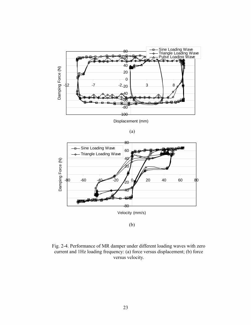
Fig. 2-4. Performance of MR damper under different loading waves with zero current and 1Hz loading frequency: (a) force versus displacement; (b) force

versus velocity.

-100

-80

-60

-40

-20

0

20

40

60

80

-12 -7 -2 3 8

Displacement (mm)

Dam

ping

For

ce (N

)

Sine Loading WaveTriangle Loading WavePulse Loading Wave

(a)

-80

-60

-40

-20

0

20

40

60

80

-80 -60 -40 -20 0 20 40 60 80

Velocity (mm/s)

Dam

ping

For

ce (N

)

Sine Loading WaveTriangle Loading Wave

(b)

23

Fig. 2-5. Performance of MR damper under different temperatures with 0.4A current and 1Hz loading frequency: (a) force versus displacement; (b) force versus

velocity.

(a)

-100

-80

-60

-40

-20

0

20

40

60

80

-12 -10 -8 -6 -4 -2 0 2 4 6 8 10 12

Displacement (mm)

Dam

ping

For

ce (N

) T=0T=10T=20T=30T=40T=50

(b)

-100-80-60-40-20

020406080

-80 -60 -40 -20 0 20 40 60 80

Velocity (mm/s)

Dam

ping

For

ce (N

)

T=0T=10T=20T=30T=40T=50

24

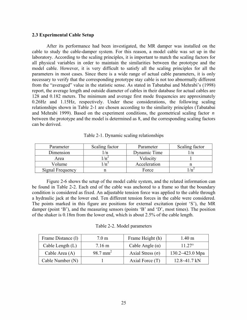
2.3 Experimental Cable Setup After its performance had been investigated, the MR damper was installed on the

cable to study the cable-damper system. For this reason, a model cable was set up in the laboratory. According to the scaling principles, it is important to match the scaling factors for all physical variables in order to maintain the similarities between the prototype and the model cable. However, it is very difficult to satisfy all the scaling principles for all the parameters in most cases. Since there is a wide range of actual cable parameters, it is only necessary to verify that the corresponding prototype stay cable is not too abnormally different from the “averaged” value in the statistic sense. As stated in Tabatabai and Mehrabi’s (1998) report, the average length and outside diameter of cables in their database for actual cables are 128 and 0.182 meters. The minimum and average first mode frequencies are approximately 0.26Hz and 1.15Hz, respectively. Under these considerations, the following scaling relationships shown in Table 2-1 are chosen according to the similarity principles (Tabatabai and Mehrabi 1999). Based on the experiment conditions, the geometrical scaling factor between the prototype and the model is determined as 8, and the corresponding scaling factors can be derived.

n

Table 2-1. Dynamic scaling relationships

Parameter Scaling factor Parameter Scaling factor Dimension 1/n Dynamic Time 1/n

Area 1/n2 Velocity 1 Volume 1/n3 Acceleration n

Signal Frequency n Force 1/n2

Figure 2-6 shows the setup of the model cable system, and the related information can be found in Table 2-2. Each end of the cable was anchored to a frame so that the boundary condition is considered as fixed. An adjustable tension force was applied to the cable through a hydraulic jack at the lower end. Ten different tension forces in the cable were considered. The points marked in this figure are positions for external excitation (point ‘S’), the MR damper (point ‘B’), and the measuring sensors (points ‘B’ and ‘D’, most times). The position of the shaker is 0.18m from the lower end, which is about 2.5% of the cable length.

Table 2-2. Model parameters

Frame Distance (l) 7.0 m Frame Height (h) 1.40 m Cable Length (L) 7.16 m Cable Angle (α) 11.27° Cable Area (A) 98.7 mm2 Axial Stress (σ) 130.2~423.0 Mpa

Cable Number (N) 1 Axial Force (T) 12.8~41.7 kN

25

7.0m

1.17m

G

A

F E

C B D

α

7.16m

Jack

Anchor Anchor

1.40m

Cable experimental setup.Fig. 2-6.

0.58m1.75m 1.17m 0.58m 1.75m

2.4 Cable Vibration without MR Damper To measure the natural frequency of the cable, a mass was hung at the middle point

‘D’ and the string connecting the mass was cut to give an excitation to the cable for a free vibration. The acceleration time histories at points ‘B’ and ‘D’ were measured by two accelerometers and collected by a Photon® data acquisition system. FFT (Fast Fourier Transform) of those time history data is carried out to obtain the power spectral density (PSD). The fundamental natural frequency was obtained as 8.93 Hz when the cable axial tension force was 16.06 kN. Since the scaling factor used is eight, the frequency of the prototype cable thus corresponds to 1.12Hz, which is within the reasonable range of the actual cable frequency (Tabatabai et al. 1998). Theoretically, the natural frequency can be calculated by the following equations (Irvine 1981) LmTf π2Ω= , (2-2) where is the solution of a transcendental equation as Ω , (2-3) 32 )2/)(/0.4(2/)2/tan( Ω−Ω=Ω λwhere )/()/)cos(( 22 EATLLTmgL eαλ = (2-4) (2-5) LTmgLLe )8/)/)cos((1( 2α+=

In these equations, E is the Young’s modulus, T is the tension force of the cable, L is

the cable length, α is the cable inclination angle, is the deformed cable length (assumed as a parabolic deflected shape), is the cross section area, is the mass per unit cable length, and is a non-dimensional parameter to describe the dynamic behavior of the cable, which is proportional to the ratio of the axial stiffness to the geometric stiffness.

eLA m

2λ

26

From Eqs. (2-2) to (2-5) the frequency is calculated as 10.08Hz, which is 12.9% higher than the experimental result. The theoretical and experimental frequencies versus tension forces are plotted in Figure 2-7. Both the theoretical and the experimental results show that the cable natural frequency increases with the increase in the tension force. Another main purpose of this simple comparison between the experimental and analytical results is to verify the experimental procedure including data acquisition and processing.

f

02468

1012141618

0 10000 20000 30000 40000 50000

Tension Force (N)

Freq

uenc

y (H

z)

ExperimentalTheoretical

Fig. 2-7. Predicted and measured cable natural frequencies.

2.5 Cable Free Vibration Control with MR Damper After testing the cable by itself, the MR damper was then connected to point ‘B’ to

reduce the cable vibration. The acceleration time history of the cable mid-span point ‘D’ is plotted in Figure 2-8, in which all the data are normalized for the convenience of comparison. It is observed from Figure 2-8(a) that the damper provides a considerable damping even if it is in its passive mode (a = 0A); it damps out the cable vibration rather quickly. Figure 2-8(b) shows that when the current reaches 0.1A, the acceleration response is reduced more quickly than the passive mode case. Figure 2-8(c) shows the acceleration time history data with currents of 0.1A and 0.2A from 0s to 1.5s in detail. It is observed that the damper with a 0.2A current reduces the vibration slightly more efficiently than that with a 0.1A current does at the beginning when the vibration is large and is almost the same after 0.5s when the vibration is small. This occurs because, on one hand, when the measured signals are small, the relative error due to the noise gets bigger. On the other hand, since the MR damper can be considered as a Bingham element, it needs a bigger force (or vibration) to overcome the Coulomb friction to pull and push the damper when the current becomes larger. If the driving force provided by the cable vibration is not large enough, the MR damper works as a fixed support (or called locked) and the damping effect under different currents beyond some critical current is the same. This phenomenon is called the saturation effect of MR dampers.

27

2.6 Cable Forced Vibration Control with MR Damper Instead of using the hanging mass, a shaker working as an excitation source was

placed at 0.18m away from the lower end of the cable in the forced vibration tests. This distance is 2.5% of the whole cable length. This shaker can provide several different excitations including sine waves, triangular waves, and white-noise waves. Sine waves are used extensively in this study.

Figure 2-9 shows the cable acceleration with a 10Hz sine wave excitation. From this

figure it is observed that the cable vibration with a damper of 0.1A current is much less than that without a damper. The ratio of the vibration peak values between the cable without a damper and the cable with a damper at a 0.1A current is about 14.

Figure 2-10 shows the peak acceleration response of different frequencies where all

the peak values are normalized by that without a damper for every excitation frequency. The cable tension force is 16.06 kN correspondingly, and the measured cable frequency is 8.93Hz. This figure shows that the reduction effect is the best at the 9Hz excitation, which corresponds to the resonant frequency of the cable-damper system. The reduction effect decreases when the excitation frequency is significantly different from this resonant frequency.

Figure 2-11 shows the reduction efficiency around the resonant frequency for different

currents. It is observed that the resonant frequency (the frequency corresponding to peak value) increases slightly with the increase in current. This implies that when the current in the MR damper increases, the stiffness of the damper, and therefore, the natural frequency of the cable-damper system become larger. This phenomenon is known as frequency shift. This frequency shift is similar to the observation of a conventional viscous damper added to the cable end (Main and Jones 2002). 2.7 Conclusions

The following conclusions can be drawn based on the present experimental study: (1) MR dampers can provide considerable damping forces, even at their passive mode

(with zero current), and have a large dynamic range. The damper used in this study has a maximum damping output force of 10N at the passive mode and about 80 N at the maximum current of 0.5A, corresponding to a dynamic range of about 8 under the sine loading wave with a frequency of 1Hz and an amplitude of 10mm for the displacement control experiment.

(2) MR dampers can provide almost the same damping force for a large range of

frequencies from 0.5Hz to 5Hz when the current in the MR damper is large. When the current is small, the damping force increases slightly with the loading frequency.

28

Fig. 2-8. Time history acceleration response of cable with MR damper: (a) no damper versus zero current; (b) no damper versus 0.1A current; (c) 0.1A

current versus 0.2A current.

-1.000-0.800-0.600-0.400-0.2000.0000.2000.4000.6000.8001.000

0.000 0.500 1.000 1.500

Time (s)

Acc

eler

atio

n

a=0.1Aa=0.2A

(c)

(a)

-1.000-0.800-0.600-0.400-0.2000.0000.2000.4000.6000.8001.000

0.000 1.000 2.000 3.000 4.000 5.000 6.000

Time (s)

Acc

eler

atio

n

No dampera=0A

-1.000-0.800-0.600-0.400-0.2000.0000.2000.4000.6000.8001.000

0.000 1.000 2.000 3.000 4.000 5.000 6.000

Time (s)

Acc

eler

atio

n

No dampera=0.1A

(b)

29

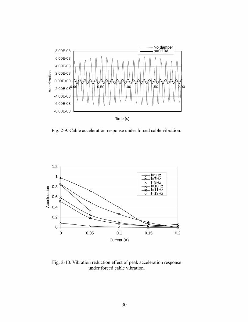
Fig. 2-9. Cable acceleration response under forced cable vibration.

-8.00E-03

-6.00E-03

-4.00E-03

-2.00E-03

0.00E+00

2.00E-03

4.00E-03

6.00E-03

8.00E-03

0.00 0.50 1.00 1.50 2.00

Time (s)

Acc

eler

atio

nNo dampera=0.10A

Fig. 2-10. Vibration reduction effect of peak acceleration response under forced cable vibration.

0

0.2

0.4

0.6

0.8

1

1.2

0 0.05 0.1 0.15 0.2

Current (A)

Acc

eler

atio

n

f=5Hzf=7Hzf=9Hzf=10Hzf=11Hzf=13Hz

30

Fig. 2-11. Vibration reduction effect and frequency shift of peak acceleration response under forced cable vibration.

-0.0050

0.0050.01

0.0150.02

0.0250.03

0.0350.04

0.045

0 2 4 6 8 10 12 14

Frequency (Hz)

Acc

eler

atio

n

No dampera=0Aa=0.05Aa=0.10Aa=0.15Aa=0.20A

(3) The curve shape and size of the output damping force versus the displacement loop

of MR dampers is almost the same if the loading wave is smooth. However, when the loading wave is sharp, such as for an impulse loading, the corresponding curve loop has a much smaller area that represents the dissipated energy when the maximum movement of the damper is preset.

(4) The working temperature does have some effect on the performance of MR

dampers, especially between 20°C and 30°C. (5) MR dampers are a good choice for adding supplementary damping to reduce the

cable vibration both for free vibration and forced vibration. The vibration reduction efficiency increases with the increase in the current. However, there is a saturation current beyond which the reduction effect will be the same.

(6) MR dampers can help reduce cable vibrations under a variety of excitation

frequencies. The reduction effect is extraordinarily efficient for the resonant vibration case when the large output damping force can be fully exerted.

(7) With the installation of MR damper on the cable, the natural frequency of the

cable-damper system increases slightly with the increase in the current. 2.8 References Angelo, W. J., 1997, “Lasers ensure stay cable safety,” Engineering News-Record, July 28,

p10.

31

Christenson, R. E., Spencer, B. F. Jr. and Johnson, E. A., 2002, "Experimental studies on the smart damping of stay cables," in Proceedings of 2002 ASCE Structures Congress, Denver, Colorado, USA, April 4-6.

Ciolko, A.T., and Yen, W. P., 1999, “An immediate payoff from FHWA’s NDE initiative,”

Public Roads, May/June, 6, 10-17. Dyke, S.J., Spencer, B.F., Jr., Sain, M.K., and Carlson J.D, 1996a, “Seismic response

reduction using Magnetorheological dampers,” in Proceedings of the Thirteenth Triennial World Congress, International Federation of Automatic Control, San Francisco, CA, June/July, Vol. L, pp. 145-150.

Dyke, S.J., Spencer, B.F., Sain, M.K., and Carlson, J.D., 1996b, “Modeling and control of

Magnetorheological dampers for seismic response reduction,” Smart Materials and Structures, 5, 565-575.

Dyke, S. J., 1998, "Seismic protection of a benchmark building using Magnetorheological

dampers," in Proceedings of the 2nd World Conference on Structure Control, Kyoto, Japan, June 29-July 2.

Flamand, O., 1995, “Rain-wind induced vibration of cables,” Journal of Wind Engineering

and Industrial Aerodynamics, 57, pp. 353-362. Irvine, H.M., 1981, Cable Structures, The MIT press, Cambridge, MA. Johnson, E.A., Baker, G.A., Spencer, B.F., Jr., and Fujino, Y., 2001, “Semiactive damping of

stay cables neglecting sag,” Technical Report No. USC-CE-01EAJ1, University of Southern California, Los Angeles, Ca.

Johnson, E. A., Baker, G. A., Spencer, B. F., Jr., and Fujino, Y., 2005, "Semiactive damping

of stay cables," Journal of Engineering Mechanics. In press. Langsoe, H. E., and Larsen, O. D., 1987, “Generating mechanisms for cable stay oscillations

at the FARO bridges,” in Proceedings of the International Conference on Cable-stayed Bridges, Bangkok, November 18-20.

Lord Corporation, 2004a, http://www.lord.com/DesktopDefault.aspx?TabID=437. Lord Corporation, 2004b, http://www.lord.com/Default.aspx?tabid=1127&page=1&-

docid=684. Lord Corporation, 2004c, http://www.lord.com/Default.aspx?tabid=763. Lord Corporation, 2004d, http://www.lord.com/Default.aspx?tabid=767.

32

Lou, W. J., Ni, Y. Q., and Ko, J. M., 2000, "Dynamic properties of a stay cable incorporated with Magnetorheological fluid dampers," Advances in Structural Dynamics, J.M. Ko and Y.L. Xu (eds.), Elsevier Science Ltd., Oxford, UK, Vol. II, pp. 1341-1348.

Main, J. A., and, Jones, N. P., 2002, "Free vibration of taut cable with attached damper. I:

linear viscous damper," Journal of Engineering Mechanics, 128(10), 1062-1071. Phelan, R. S., Mehta, K. C., Sarkar, P.P. and Chen L., 2002, Investigation of Wind-Rain-

Induced Cable-Stay Vibrations on Cable-Stayed Bridges, Final Report, Center for Multidisciplinary Research in Transportation, Texas Tech University, Lubbock, Texas.

Spencer Jr., B.F., Dyke, S.J., Sain, M.K., and Carlson, J.D., 1997, “Phenomenological model

for Magnetorheological dampers,” ASCE Journal of Engineering Mechanics, 123(3), 230-238.

Stanway, R., Sproston, J.L., and Stevens, N.G., 1985, Non-linear identification of an

electrorheological vibration damper, IFAC Identification and System Parameter Estimation, pp. 195-200.

Stanway, R., Sproston, J.L., and Stevens, N.G., 1987, “Non-linear modeling of an

electrorheological vibration damper,” Journal of Electrostatics, 20, 167-184. Tabatabai, H., Mehrabi, A.B., Morgan, B.J., and Lotfi, H.R., 1998, Non-destructive Bridge

Evaluation Technology: Bridge Stay Cable Condition Assessment, Final report submitted to the FHWA, Construction Technology Laboratories, Inc., Skokie, IL.

Tabatabai, H., and Mehrabi, A. B., 1999, Tuned Dampers and Cable Fillers for Suppression of

Bridge Stay Cable Vibrations, Final report to TRB IDEA program, Construction Technology Laboratories, Inc, Skokie, Illinois.

Tabatabai, H., and Mehrabi, A. B., 2000, “Design of mechanical viscous dampers for stay

cables,” Journal of Bridge Engineering, 5(2), 114-123. Yi, F., Dyke, S.J., Caicedo, J.M., and Carlson, J.D., 2001, “Experimental verification of

multi-input seismic control strategies for smart dampers,” ASCE Journal of Engineering Mechanics, 127(11), 1152-1164.

Yoshioka, O., Dyke, S. J., Giacossa, L. M. and Truman, K. Z., 2002, ”Torsional response

control of asymmetric building using smart dampers,” in Proceedings of 15th ASCE Engineering Mechanics Conference, Columbia University, New York, NY, June 2-5.

33

CHAPTER 3. CABLE VIBRATION CONTROL WITH A SEMIACTIVE MR DAMPER

3.1 Introduction

Stay cables are susceptible to external disturbances because of their inadequate

intrinsic damping. Under certain combinations of light rain and moderate wind (about 10 to 15 m/s), incidences of large-amplitude vibrations (on the order of 1 to 2m) of stay cables have been reported worldwide (Ciolko and Yen 1999, Main and Jones 2001). This phenomenon is known as wind-rain induced cable vibration. Excessive cable vibrations are a potential threat to public safety and the national investment in transportation infrastructures. This issue has raised great concern in the bridge community and has been a cause of deep anxiety for the observing public.

Other than adding crossing ties/spacers to enhance the system damping for the cable

network (Langsoe and Larsen 1987) or treating the cable surface to increase the cable aerodynamic stability (Flamand 1995, Sarkar et al. 1999), mechanical dampers are broadly used to mitigate cable vibrations. As a passive control method, oil/viscous dampers have been extensively studied to improve the damping for stay cables, both theoretically and practically (Carne 1981, Watson and Stafford 1988, Yoshimura et al. 1989, Pacheco et al. 1993, Krenk 2002, Main and Jones 2002). However, passive dampers may not be able to provide enough damping for long stay cables since they are restricted to an anchorage close to the lower cable end for aesthetic and installation reasons. For the passive mechanical damper to be effective, it is commonly believed that it should be anchored a certain distance away from the cable end. The further away the damper, the more damping it provides. A rule of thumb is that for a 1% damping, the damper should be 2% of the cable length away from the cable end for the first mode.

One promising way to overcome the constraints of the passive mechanical dampers is

to use the TMD-MR damper proposed by Cai et al. (2005). Cai et al. (2006) established the governing equation for the cable-TMD-MR damper system, and Wu and Cai (2006b) conducted a thorough parametric study for the effect of cable and damper parameters on the damper performance. Results show that the TMD-MR damper can provide much more damping than the viscous damper for a targeted mode (Cai and Wu 2006).

Another way is to use semiactive mechanical dampers, as recommended by Johnson et

al. (2003) after his series research via a simulation approach on the performance of passive, semiactive, and active dampers installed to cables (Johnson et al. 1999, Johnson et al. 2002, Johnson et al. 2003). They built a sagged cable model with passive, semiactive, and active dampers and developed a control-oriented model using a combination of cable static shape and sinusoid series shape functions. Their results show that reduction in root mean square (RMS) response can be achieved 10% to 50% better than the optimal passive linear damper if the semiactive dampers are not placed at any node of the cables. The cost of better damping performance is a larger output damper force, approximately 5-10 times larger depending on the damper locations.

34

With the ability to adjust the output damping force, Magnetorheological (MR) dampers are a good choice to fulfill the semiactive control strategy. The first real application of MR dampers for cable vibration control has been installed in the Dongting Lake Bridge, China. However, the adjustable feature of the MR dampers is not fully utilized (Chen et al. 2003, Lord Corporation 2004). They have actually been used as cost-effective passive dampers. Therefore, experimental investigation is necessary for the guidance of their real application in the near future. This study is aimed to carry out experimental investigation to eliminate the gap between the simulation and the implementation. The control-oriented cable-damper model will be reviewed, and controllers that can work with hardware will be demonstrated. Comparisons are focused on the cable response and output damper forces between cables with and without semiactive dampers, control performance between different control methods, and control performance for semiactive MR dampers with different maximum currents. 3.2 State-Space Equation and Control Strategy

The cable-damper calculation model is shown in Fig. 3-1. The MR damper is placed at

an intermediate point , dividing the cable into two segments. The notation without subscript is used to represent either cable segment. The Cartesian coordinate system is also indicated in this figure. The left support of the cable is taken as the origin for the first segment and the right support for the second segment. Thus, the governing equation for the taut cable vibration with a damper can be written as

dx

tvc

tvmxxFxxF

xvHf ssddy ∂

∂+

∂

∂=−+−+

∂

∂+

2

2

2

2)()(

cosδδ

θ (3-1)

where is the distributed cable force along the y direction; yf H is the horizontal component of the static tension force; θ is the inclined cable angle measured from the horizontal axis; is the cable dynamic displacement component along the y coordinate measured from the static equilibrium position of the cable; and are the output damping force of the MR damper and the reaction force of the shaker, respectively;

v

dF sF)(•δ is the Direc delta function; and

are the damper and shaker locations, respectively; m and are the distributed cable mass and damping coefficient per unit length, respectively; is the time; the notation

dx sxc

t)()(od

d • denotes the

derivative of “ ” with respect to “ ”; and • o)()(o∂•∂ means the partial derivative of “ • ” with

respect to “ ”. o

According to the standard Galerkin’s method, any shape function φ that satisfies the

boundary conditions 0)()0( == lφφ can be chosen to solve the governing equation (3-1). Usually, the following sinusoid shape functions can be used ljxx /sin)( πφ = . (3-2)

35

To build up an accurate and efficient control-oriented model for applications, the

number of shape functions is an important consideration since each shape function is actually one degree of freedom (DOF) in the generalized dynamic equation. Too many shape functions may cause the semiactive computation of the controller to become impractical. Pacheco et al. (1993) uses sinusoid shape functions only, which need 350 DOFs to obtain accurate results. Xu and Yu (1998) proposed a hybrid method with finite element technology, which also requires numerous DOFs. Johnson et al. (2003) suggested using the static cable profile as one of the shape functions, as well as the sinusoid shape functions. This approach largely reduced the number of required shape functions, which insured the successful semiactive control strategy with a low order, control-oriented model. Based on the simulation study (Johnson et al. 2003), 21 terms, including one triangle shape function for the damper effect and 20 sinusoid functions, could provide better accuracy than several hundred sinusoid-only terms.

For the taut cable considered in the current experimental study, the following two

triangle shape functions are used to count for the effect of the damper and the shaker, respectively

(3-3-a) ⎩⎨⎧

≤≤−−≤≤

=lxxxlxl

xxxxx

dd

ddd ),/()(

0,/)(φ

. (3-3-b) ⎩⎨⎧

≤≤−−≤≤

=lxxxlxl

xxxxx

ss

sss ),/()(

0,/)(φ

Similarly to Johnson’s work, 20 sinusoid functions are used. With these shape functions, the displacement of the cable can be computed as

(3-4) 22...1)()(),(1

== ∑=

kxtqtxvk

jjj φ

Submitting Eq. (3-4) and the corresponding shape functions into Eq. (3-1), since the

distributed force is not considered in the current study, the generalized discrete dynamic equation for the cable-MR damper system can be written as )Φ(xF)Φ(xFKqqCqM ddss +=++ &&& . (3-5)

Fig. 3-1. The control-oriented inclined cable model.

damper

y

x

xs

xd

shaker

36

The contents of the mass matrix M , the damping matrix , and the stiffness matrix CK can be found in Johnson et al. (2002) for the taut cable model. The damping matrix C is proportional to the mass matrix and can be determined by the distributed c value. A small first modal damping of 0.5% for the generalized mode is assumed to avoid infinite resonant response, from which the N·s/m2 and modal damping for other modes can be obtained. is the external loading simulated by the shaker force, which has the feature of white noise. and are the load vectors for the excitation force and the damper force, respectively. Their contents are the values of the shape functions in Eq. (3-2) and (3-3) at and , as,

0.378=csF

)Φ(xs )Φ(xd

sx dx (3-6-a) T

ssdss lxlxxx ])/20sin()/sin(/1[ ππ L=)Φ(x (3-6-b) T

ddsd lxlxxx ])/20sin()/sin(1)1/()1[( ππ L−−=)Φ(xd

q , , and are the generalized displacement, velocity, and acceleration, respectively. Thus, the state space equation and the output equation for the control-oriented model can be written as

q& q&&

(3-7-a) sd EFBFAZZ ++=&

vFGFDZCY sd +++= yyy (3-7-b) where is the state variable; Y is the output vector that can be measured by the accelerometers; and is the noise vector from the measurement. Other matrices can be obtained as

T]q[qZ &=

v

(3-8-a) ⎥⎦

⎤⎢⎣

⎡−−

= −− CMKMI0

A 11 ⎥⎦

⎤⎢⎣

⎡= − )Φ(xM

0B 1

d⎥⎦

⎤⎢⎣

⎡= − )Φ(xM

0E

s1

[ ]CΦMKΦMC 11y

−− −−= [ ])Φ(xΦMD d1

y−= [ ])Φ(xΦMG s

1−=y , (3-8-b) since only accelerations are used for the feedback loop. The contents of Matrix Φ can be determined by the placement and number of the accelerometers.

For the semiactive control with a MR damper, two correlated controllers should be designed (Johnson et al. 2003). The primary Linear Quadratic Gaussian (LQG) controller is designed to minimize the following cost function

∫ ++=∞→

Tp

dTdtFR

TEJ

0

2 )))((1(lim qMq21Mqq

21 TT && , (3-9)

where the parameter R represents the variable control weight for the feedback force of the MR damper.

With a force feedback proportional to the estimated system state, , the

primary feedback gain can be obtained as ZLF ˆ−=p

d

PBL T1−= R , where satisfies the algebraic Riccati equation

P

(3-10) 0QPBPBPAPA TT =+−+ −1R

and . ⎥⎦

⎤⎢⎣

⎡=

0.5M000.5M

Q

37

The following Kalman filter is used to estimate the system state (3-11-a) )Y(YLBFZAZ kfd

ˆˆˆ −++=&

(3-11-b) dyy FDZCY += ˆˆ

where is the estimator gain. Similarly, the matrix satisfies the algebraic Riccati equation

1Tykfykf

Tykf

Tykfkf )GQG)(RGEQC(PL −++=

kfP0EEQ)EQGP(C)GGQ)(RGEQC(PAPAP T

kfT

kfykfy1T

ykfkfTykf

Tykf

Tkfkf =++++−+ −

(3-12) where and are the auto excitation and noise spectral density, respectively. The expectations for the excitation and the noise are required to be zero to apply the algorithm.

kfQ kfR

The MR damper used in this control-oriented strategy and simulation can be expressed by the following Bingham model (Stanway et al. 1985) )( ddyddd vsignFvCF && += (3-13) where is the damping coefficient, is the damper velocity, is the friction force, which is related to the applied current in the MR damper, and

dC dv& dyF)(•sign means the sign of the

corresponding quantity. All these parameters can be obtained from the experimental data in Wu and Cai (2006b). The values of parameters and used in the simulation section are 100 N·s/m and 60 N, respectively. Fig. 3-2 shows the output force calculated by using Eq. (3-13) and the experimental data. Only one cycle of data is plotted in the two bottom figures for clarity reasons.

dC dyF

Fig. 3-2. Bingham model and experimental data.

-10 -5 0 5 10-100

-50

0

50

100

Displacement (mm)

Out

put

forc

e (N

)

-200 -100 0 100 200-100

-50

0

50

100

Velocity (mm/s)

Out

put

forc

e (N

)

-10 -5 0 5 10-100

-50

0

50

100

Displacement (mm)

Out

put

forc

e (N

)

-200 -100 0 100 200-100

-50

0

50

100

Velocity (mm/s)

Out

put

forc

e (N

)

ExperimentalBingham

38

Since the MR damper can only employ dissipative force, the output damping force must be of a different sign than the damper velocity. Therefore, the secondary controller for this particular feature can be presented by the following equation , (3-14) )(max d

pd vFII &−Η=

where I is the command current sent to the MR damper; is the maximum current that can be applied to the damper; and

maxI)(•Η is the Heaviside function, or unit step function. In this

experiment, the damper velocity can be obtained by integrating the corresponding acceleration.

dv&

3.3 Simulation Results Before the experimental verification, computer simulation is carried out in Simulink/Matlab to determine suitable parameters for the primary controller. Extensive simulation work can be found in Johnson et al. (2003). The simulation done here focuses on the cable control problem at hand. The selected controller should provide a satisfactory control effect and make the feedback force in the range of the capacity of the real MR damper used. A block diagram for the entire controlled system is plotted in Fig. 3-3, which embodies the concept in section 3.2. Table 3-1 gives a simple comparison between the control effects of some different control strategies, including active control, optimal ordinary passive control, control with a MR damper in passive mode (MR damper with constant zero current), and semiactive control with a MR damper via the LQG control algorithm. The dispσ is a quantity representing a mean displacement integrated along the cable, as defined by the following equation (Johnson et al. 2003)

∫∫ ≈==exp

0exp0

2 ˆˆ1][]),([T

TTl

disp dtT

EdxtxvE qMq(t)Mq(t)qσ (3-15)

The last approximation comes from the factor that the expected value of an ergodic quantity is equal to its time average. The state can be estimated from a similar Kalman filter with Eq. (3-11-a). However, the output equation should change to the following equation

q̂

. (3-16) Z0Iq ˆ][ˆ =

Table 3-1. Cable vibration control with different methods

Active Optimal passive viscous damper MR passive mode MR semi

σdisp (mm) 1.033 1.626 1.387 1.223 Fd

rms (N) 9.24 8.34 8.55 43.78 Fd

max (N) 24.33 20.78 20.80 80.38

39

Fig. 3-3. Block diagram for the controlled system.

MR damper Cable

Primary controller

Secondary controller

Shaker

Fdp

I Y

Fd Fs

Integration dv&

From Table 3-1, it can be seen that the semiactive control method with MR damper

can provide another 24.8% off of the integrated displacement, compared to that of the optimal passive dampers (1.223 vs. 1.626mm). Even the MR passive mode can still provide a better control effect than the optimal passive viscous dampers. The control effect by a semiactive MR damper is not as good as that of an active control, but in a limited difference. The active control can provide another 36.5% off of the integrated displacement, also compared to that of the optimal passive dampers (1.033 vs. 1.626mm). The predicted damper output force Fd

rms is much larger than that of the active control method, which implies that the full damper output force is too large for the present cable vibration. Another possible reason comes from the factor that the damper model Eq. (3-13) is not perfectly accurate. Therefore, several smaller applied maximum currents are chosen in the experimental verification. maxI 3.4 Experimental Setup

Scaling principles call for maintaining the similitude between the prototype cable and the model cable. However, it is actually very difficult to satisfy all the scaling principles for all the parameters in most cases. Since there is a wide range of actual cable parameters, it is only necessary to verify that the corresponding prototype stay cable is not abnormally different from the “average” value. Therefore, with considering the limitations of the laboratory facility, the scaling factor between the prototype and the model is determined as 8 according to the scaling relationship in Wu and Cai (2006b).

n

Table 3-2. Model cable parameters

Cable Length ( ) l 7.16 m Cable Angle (θ ) 11.27° Cable Area (A) 98.7 mm2 λ2 vale 0.059

xd 2.01 m xs 0.79 m

40

Fig. 3-1 shows the setup of the cable model and the related information can be found in Table 3-2. Each end of the cable is anchored to a frame so that the boundary conditions are considered fixed. An adjustable tension force is applied to the cable by a hydraulic jack (Fig 3-4), which can be measured accurately by a load cell (Fig 3-5) with a capacity of 44480N (10kips). The tension force is acquired by the DastarNet data acquisition system from Gould Inc. Thus, a range of the geometry-elasticity values can be achieved by varying the tension force. However, in the current study, a constant tension force of 9438.7 N is used, which corresponds to a vale of 0.059. This value is in the range of 0.008-1.08, a range that covers 90% of real cables based on the database collected by Tabatabai et al. (1998).

2λ

Fig. 3-4. Hydraulic jack. Fig. 3-5. 10 kips load cell. The V408CE shaker (Fig. 3-6) from Ling Dynamic System Inc. located at

(11% of the cable length) is used to generate the excitation for the cable vibration. The maximum output force from the shaker for a sine-wave excitation is 98N. A frame is built to facilitate the installation of the shaker perpendicular to the cable. Different forms of the excitation force can be applied by the shaker, with the magnitude measured by a load cell between the cable and the shaker. As required by the control strategy, a bandlimited white noise excitation generated from the Simulink software is used and sent to the shaker in the experiment. Before the signal goes into the shaker, a fourth order bandpass filter is used to shape the spectral content of the input energy to excite the first cable vibration mode. The transfer function of the filter can be expressed as

m 0.79=sx

222

4

)3.0( ff

fsf ss

Hωω

ω++

= . (3-17)

The MR damper type RD-1097-01 (Fig. 3-7) purchased from Lord Cooperation is

used as the semiactive damper, which can provide a maximum force level of ±80N at a maximum current of 0.5 ampere (Wu and Cai 2006b). The damper is located at

(28% of the cable length). It is noted that the damper position here does not m 01.2=dx

41

represent most actual applications. Similarly, a frame is provided to make the MR damper perpendicular to the cable chord and to investigate the performance of the MR damper at different locations if necessary. A load cell is placed between the damper and the cable to measure the real force that the MR damper provides.

Two miniature accelerometers (Fig. 3-8) from PCB Piezotronics Inc. are used to measur

These two accelerations used for the controllers are acquired by a MultiQ-PCI board from Q

Fig. 3-6. LDS shaker.

Fig. 3-7. MR damper.

e the cable vibration response at different places. These accelerometers can measure up to ±4900m/s2 acceleration with a resolution of 0.02m/s2 RMS value. These accelerometers are also used to provide input information for the Kalman filter to estimate the full state in the primary controller. One of them is at the mid-span (3.58m) and the other is used to measure the damper acceleration, which also provides the damper velocity for the secondary controller after integration. Low pass filters with a cut off frequency of 30Hz are used to get rid of the noise before the accelerations are used.

uanser Inc. This board has four available AD converters and 16 DA converters, which can accept a maximum voltage of ±10V input and output signals. With the Wincon realtime control software built in Simulink/Matlab, this board can fulfill a realtime control task seamlessly. Actually, it works as an interface between the control algorithms simulated in Matlab and the controlled structures. All the signals (two accelerations, the forces from the shaker and the damper) are acquired for the post processing to compare the cable response and the output damping force between the cable with and without the semiactive damper.

42

Fig. 3-9. Acquisition system. Fig. 3-8. PCB accelerometer. 3.5 Experiment Results

The experiment is carried out to verify the control strategies explained previously. As stated in Eqs. (3-11-a), (3-15), and (3-16), the main criteria for the comparison, the integrated displacement along the cable, can be obtained by the Kalman estimator from the two measured accelerations.

Five experiments are carried out to demonstrate the effectiveness of the semiactive

control, as indicated in Table 3-3. Before the MR damper is added to the cable, the cable vibration is measured under an excitation force of 13.09N RMS. The integrated displacement along the cable is 2.65mm. When the MR damper is installed but is not applied with current, the integrated displacement is reduced to 1.29mm, 51% less than the uncontrolled displacement. This indicates that even if the MR damper is in its passive mode, it can still provide a considerable performance for the cable vibration. Therefore, a MR damper can work as a fail-safe device for the control strategy. The output damping force for the MR damper in passive mode is very low. When the MR damper is working as a semiactive device, generally it can provide a better control performance. When the applied current is set as 0.1A, the integrated displacement is further reduced to 0.22mm, 92% less than the uncontrolled displacement. Further increasing the current may result in a better performance, but enhanced performance is not guaranteed. As the current is increased from 0.1A to 0.2A, better damper performance is achieved by reducing the displacement from 0.22mm to 0.082mm. However, the performance becomes worse when the current changes from 0.2A to 0.3A. Please note that the Fd

max for the semiactive MR damper with 0.2A current is 26.77N, which is around the simulation prediction of 24.33N for the active control. This observation suggests that the MR damper may achieve the best control when its output capacity is set around its active control counterpart. Increasing the output capacity may not be beneficial to the control effect since the MR damper force may be too large for the cable vibration for a certain level of excitation.

maxI

43

Table 3-3. Damper performance

σdisp (mm) Fdrms(N) Fd

max(N) Fsrms(N)

Uncontrolled 2.65 N/A N/A 13.09 MR passive mode 1.29 (51%) 4.96 13.19 15.39

Semi 0.1A 0.22 (92%) 6.54 20.45 17.15 Semi 0.2A 0.082 7.57 26.77 17.27 Semi 0.3A 0.090 7.99 34.44 17.53

The time history records for the measured accelerations at the damper location and the cable middle point are plotted in Fig. 3-10. Apparently, the semiactive MR damper gives a much better performance to reduce the cable vibration at both sensor locations.

Fig. 3-10. Time history records for both sensors with different control strategies.

0 5 10 15 20 25 30 35 40 45 50-10

-5

0

5

10

Time (s)

Dap

mpe

r acc

e (m

/s2 )

0 5 10 15 20 25 30 35 40 45 50-10

-5

0

5

10

Time (s)

Mid

dle

poin

t acc

e (m

/s2 )

Uncontrolled MR passive mode Semi 0.2A

3.6 Conclusions The current study mainly discusses the experimental verification of a semiactive control approach to reduce cable vibration. The control-oriented state-space equation and the LQG control strategy are reviewed. Preliminary simulation results are obtained to design proper controller parameters and make sure the demand damper force matches the real MR damper. Experimental verification is carried out to demonstrate the idea of the semiactive

44

control. Based on the simulation and experiment results, the following conclusions can be made: 1. From the simulation results, the semiactive control can achieve a better control effect than its optimal passive counterpart and similar control effect to its active counterpart for the cable vibration reduction. Better performance is achieved by the cost of larger control forces. 2. From the experiment results, even when the MR damper is in the passive mode, it still can provide a considerable control effect. Therefore, a semiactive MR damper can be a fail-safe device when the control device is not working properly for any reason in the field. 3. Also from the experimental results, the output damping force of the semiactive damper should be set around the active demand at certain excitation levels. Otherwise, the damper output damping force may be too large for the cable vibration, which may cause a worse control effect. Therefore, future work may consider a refined control strategy for the secondary controller, which should provide different output current according to the severity of the cable vibration. 3.7 References

Cai, C.S., Wu, W.J. and Araujo, M. (2005) “Cable Vibration Control with a TMD-MR

Damper System: Experimental Exploration.” Proceedings of McMat2005, 2005 joint ASME/ASCE/SES Conference (CD), June 1-3, 2005, Baton Rouge, Louisiana, USA.

Cai, C. S., Wu, W. J. and Shi, X. M. (2006) “Cable vibration reduction with a hung-on

TMD system: theoretical study.” Journal of Vibration and Control (Accepted). Cai, C. S., and Wu, W. J. (2006) “Comparison between viscous damper and TMD-MR

damper on cable vibration reduction.” Paper under preparation (chapter 8). Carne, T.G. (1981) “Guy Cable Design and Damping for Vertical Axis wind Turbines.”

Report No. SAND80-2669, Sandia National Laboratories, Albuquerque, N.M. Chen, Z.Q., Wang, X. Y., Ko, J. M., Ni, Y.Q., Spencer, B.F., and Yang, G. Q. (2003).

“MR damping system on Dongting Lake cable-stayed bridge.” Smart Systems and Nondestructive Evaluation for Civil Infrastructures, San Diego, California, USA, 2-6 March 2003, pp.229-235

Ciolko, A.T., and W. P., Yen (1999). “An immediate payoff from FHWA’s NDE

Initiative.” Public Roads, May/June, 10-17. Krenk, S. and Nielsen, S. R. (2002). “Vibrations of a shallow cable with a viscous

damper.” Proceedings of Royal Society (London), A458, 339-357.

45

Johnson, E. A., Spencer, B. F., and Fujino, Y. (1999) “Semiactive Damping of Stay Cables: A Preliminary Study.” Proceedings of 17th International Modal Analysis Conference, Kissimmee, Florida.

Johnson, E. A., Baker, G. A., Spencer, B. F., Jr., and Fujino, Y. (2002). “Semiactive

damping of stay cables.” Journal of Engineering Mechanics. ASCE, 128(7) Johnson, E. A., Christenson, R. E., and Spencer, B. F. Jr. (2003) “Semiactive Damping

of Cables with Sag.” Computer-aided Civil and Infrastructure Engineering, 18, 2003, 132-146.

Langsoe H. E., and Larsen, O. D., (1987) “Generating mechanisms for cable stay

oscillations at the FARO bridges” Proceeding, International Conference on Cable-stayed Bridges, Bangkok, November 18-20

Lord Corporation. (2004). http://www.lord.com/Default.aspx?tabid=1127&page=1&

docid=684, 04/20/2004 Main, J. A., and, Jones, N. P. (2001). “Evaluation of Viscous Dampers for Stay-cable

vibration mitigation” Journal of Bridge Engineering, ASCE, 6(6), 385-397 Main, J. A., and, Jones, N. P. (2002a). “Free vibration of taut cable with attached

damper. I: linear viscous damper.” Journal of Engineering Mechanics, 128(10), 1062-1071 Pacheco, B.M., Fujino, Y., and Sulekh, A. (1993). “Estimation curve for modal damping

in stay cables with viscous damper." Journal of Structural Engineering., 119(6), 1961-1979 Sarkar, P. P., Mehta, K,C., Zhao, Z.S., and Gardner, T. (1999.) “Aerodynamic approach

to control vibrations in stay-cables.” Report to Texas Department of Transportation, TX. Simulink. (2002)The MathWorks, Inc., Natick, MA. Stanway, R., Sproston, J. L., and Stevens, N. G. (1985) “Nonlinear Identification of An

Electrorheological Vibration Damper.” IFAC Indentification and System Parameter Estimation, 195-200

Tabatabai, H.， Mehrabi, A.B.， Morgan, B.J., and Lotfi, H.R. (1998) “Non-destructive

Bridge Technology: Bridge Stay Cable Condition Assessment.” Final report submitted to the Federal Highway Administration, Construction Technology Laboratories, Inc., Skokie, IL.

Watson, S.C., and Stafford. D. (1988) “Cables in Trouble.” Civil Engineering, ASCE.

58(4):38–41. Wu, W.J. and Cai C.S. (2006a) “Experimental study on MR dampers and the application

on cable vibration control.” Journal of Vibration and Control, 12(1), 67-82

46

Wu, W. J. and Cai, C. S. (2006b) “Cable vibration reduction with a hung-on TMD system: parametric study.” Journal of Vibration and Control (Accepted).

Yoshimura, T., Inoue, A., Kaji, K., and Savage, M. (1989). “A Study on the

Aerodynamic Stability of the Aratsu Bridge.” Proceedings of the Canada-Japan Workshop on Bridge Aerodynamics, Ottawa, Canada, 41–50.

47

CHAPTER 4. EXPERIMENTAL EXPLORATION OF A CABLE AND A TMD-MR DAMPER SYSTEM

4.1 Introduction

There are about 30 major cable-stayed bridges in the U.S. and about 600 worldwide

(Angelo 1997). Under certain combinations of light rain and moderate wind (about 10 to 15 m/s), incidences of large-amplitude vibrations (on the order of 1 to 2m) of stay cables have been reported worldwide, including those located in the U.S. such as Fred Hartman, Weirton-Steubenville, Burlington, and Clark bridges (Ciolko and Yen 1999, Main and Jones 2001). Those cables are otherwise stable under similar wind conditions without rain. This phenomenon is known as the so-called wind-rain induced cable vibration. Excessive cable vibrations are detrimental to the long-term health of bridges, which potentially threatens the public safety and the national investment in transportation infrastructures. This issue has raised great concerns in the bridge community and has been a cause of deep anxiety for the observing public.

Recognizing this severe condition of cable vibrations, researchers have been modestly

successful to address this problem over the years by providing traditional mechanical dampers (Xu et al. 1997, Tabatabai and Mehrabi 2000), adding crossing ties/spacers (Langsoe and Larsen 1987, Caracoglia and Jones 2002) or treating cable surface with different techniques (Flamand 1995, Phelan et al. 2002). Oil dampers and friction dampers have been extensively used due to their large damping force and easy replacement. Magnetorheological (MR) fluid based dampers are relatively new mechanical dampers known for their large adjustable damping force, stable performance, quick response, and low power supply requirement in earthquake engineering (Spencer et al. 1997a, 1997b, Dyke et al. 1996a, 1996b). With a change in the electric current provided to the damper, the output damping force of MR dampers can be adjusted. MR dampers have been extensively studied in seismic applications and have proven to be a feasible means in cable vibration control (Lou et al. 2000, Christenson et al. 2002, Johnson et al. 2003). Readers are referred to the literature for more information about the MR dampers.

The first actual application of MR dampers for cable vibration control was their

installations in the Dongting Lake Bridge, China, to dissipate energy before the cable vibrations reached a destructive level (Chen et al. 2003, Lord Corporation 2004). Nevertheless, those mechanical dampers needed to be grounded (connected to the deck) close to the lower end of the stay cable for the convenience of installation and operation (generally, 1/50~1/20 of the cable length from the cable end). As a result, the vibration reduction capacity of the MR damper was not fully utilized and even problematic in controlling three dimensional cable vibrations due to the way they were installed.

As an alternative to the conventional mechanical dampers, Tabatabai and Mehrabi

(1999) recommended tuned mass dampers (TMDs) for full-scale implementation for two major reasons. First, TMDs are observed to be more efficient than other countermeasures in damping out the free vibration. Second, TMDs can be physically installed at any location

48

along the cables so that their vibration reduction capacity can be fully exploited. Although studies on TMDs have proven their efficiency, improvements are needed since the vibration reduction effect of TMDs is usually frequency sensitive. When the excitation is a narrow-band vibration or the cable vibration is mainly from one mode, the natural frequency of TMDs can be tuned to the targeted frequency, and in this case the vibration reduction effect of TMDs is usually satisfactory. However, when the excitation is a wide-band vibration, the cable vibration is composed of several equally important modes, or the natural frequency of TMDs is away from that of the cable, the vibration reduction effectiveness will be reduced considerably. Since the natural frequency between the preset TMD and the cable may mismatch for many reasons, perhaps due to the unpredicted nonlinearity of the actual cable, the difference between the calculation model and prototype cable, and the time-dependent attribute of the cable force, it is usually difficult to achieve the expected optimal vibration reduction effectiveness in field applications.

In this study, a TMD-MR damper system is proposed to improve the TMD, and

subsequently, the dynamic characteristics of the cable-TMD-MR system are investigated experimentally. This proposed TMD-MR damper system has a combined advantage of both TMDs and MR dampers (Cai and Wu 2004). On one hand, TMDs can be put anywhere along the cable, which overcomes the deficiency of conventional mechanical dampers; on the other hand, a MR damper can absorb energy directly by providing continuously adjustable damping and can change the stiffness in a small range as well, which can help the whole damper system be effective under different vibrations. As a result, a high damping efficiency may be achieved, overcoming the drawbacks of the frequency sensitivity of the TMDs and the position restriction of the MR dampers. The present study focuses on a conceptual exploration of the TMD-MR damper system for cable vibration mitigation through an experimental approach. Analytical solutions that help understand more thoroughly the behavior of the proposed TMD-MR damper system are given in a companion study (Wu and Cai 2006). Further studies will be carried out for actual applications of the proposed concept for cable vibration mitigation.

4.2 Concept and Principle of the TMD-MR Damper System

TMDs have been studied extensively in structural vibration control. The concept of

vibration control by TMDs can be stated as follows. The interaction between any two elastic bodies can be represented by a two-mass system shown in Fig. 4-1. Under the excitation of a sinusoidal force )sin( tF ω acting on mass 1, the vibration amplitudes of this two-mass system are derived as,

22

222

2121

222

1 ))(()(

2

kmkmkkFm

X m

−−−+

−=

ωωωω

and 22

222

2121

22

2 ))((2

kmkmkkFm

X m

−−−+=

ωωω

(4-1)

where 11

21

mkm =ω and 222

2mkm =ω . It can be seen from Eq. (4-1) that when , the

vibration amplitude of mass 1 vanishes with

222

ωω =m

01 =X , and the amplitude of mass 2 is 22 kFX = .

49

m1

m1

m1

m2

Fsin(ωt)

k 1 k2

Fig. 4-1. A two-mass system

The basic concept of cable vibration control using the TMD-MR damper system is similar to the two degrees of freedom system shown in Fig. 4-1, where the cable mass and the TMD-MR system mass are represented by m1 and m2, respectively. The MR damper will provide an adjustable damping and stiffness so that the cable-TMD-MR system is better represented by Fig. 4-2. The sketch of an actually proposed TMD-MR system is shown in Fig. 4-3. When MR dampers are not used or are removed, as in Fig. 4-3, the TMD-MR damper system actually reduces to a vibration absorber, i.e., a TMD without the damping element. Though a TMD usually has a damping element, the TMD component in the present study is hereafter specially referred to as the case without the damping element to distinguish it from a TMD-MR damper that consists of both TMD and MR components.

Fig. 4-2. A two-DOF model for cable-TMD-MR system.

MR

m1

m1

m1

m2

Fsin(ωt)

k 1 k2

The eventually developed TMD-MR damper system is intended to be installed on the cable, and the vibration suppression concept is shown in Fig. 4-4. The cable vibrations are due to the excitations of tower, deck, wind-rain-cable interaction, or their combinations. Characteristics of the cable vibrations will be reflected in a spectral diagram that is processed from the information of accelerometers. Multiple peaks in the spectral diagram may be expected since the excitations of cable vibrations can be single frequency, multi-frequencies, or random. The frequency of the TMD-MR system will be tuned to the frequency corresponding to the most significant resonant vibration (highest peak) or other targeted frequency along with the adjustment of its location and damping ratio in order to most efficiently suppress the vibration.

50

MR fluids thatcan changeto semi-solid

Mass of TMD

Cable

MR damper

Inner shell

Cut to clip on cable

Accelerometer

MR fluids thatcan changeto semi-solid

Mass of TMD

Cable

MR damper

Inner shell

Cut to clip on cable

MR fluids thatcan changeto semi-solid

Mass of TMD

Cable

MR damper

Inner shell

Cut to clip on cable

MR fluids thatcan changeto semi-solid

Mass of TMD

Cable

MR damper

Inner shell

Cut to clip on cable

Accelerometer

Fig. 4-3. Sketch of a TMD-MR damper system.

The TMD-MR damper system has several advantages for the vibration control strategy. The first is the vibration absorber function, i,e., a TMD function, which is especially effective for reducing the targeted resonant vibration. In addition, when the cable natural frequency changes for whatever reason, the MR component can help slightly adjust the natural frequency of the TMD-MR damper system to match the targeted resonant excitation frequency, though the major adjustability of the MR component is its damping forces. The second is the MR damper function. When the vibration involves more than one dominating vibration mode or it is difficult to tune the TMD-MR system frequency to a specific value, the MR component can dissipate energy directly by providing a considerable output damping force. Therefore, the proposed TMD-MR damper system is promising to handle different excitations effectively. 4.3 Experimental Setup

Scaling principles call for maintaining the similitude between the prototype cable and the cable model. However, it is actually very difficult to satisfy all the scaling principles for all the parameters in most cases. Since there is a wide range of actual cable parameters, it is only necessary to verify that the corresponding prototype stay cable is not abnormally different from the “average” value. Under these considerations, the scaling relationships shown in Table 4-1 are chosen according to the similitude principles (Tabatabai and Mehrabi 1999). Considering the limitations of the laboratory facility, the scaling factor n between the prototype and the model is determined as 8.

51

Table 4-1. Dynamic scaling relationships

Parameter Scaling factor (model/ prototype) Parameter Scaling factor

(model/ prototype) Dimension 1/n Dynamic Time 1/n

Area 1/n2 Velocity 1 Volume 1/n3 Acceleration N

Signal Frequency n Force 1/n2

Fig. 4-4. Sketch of cable vibration control strategy.

Fig. 4-5 shows the setup of the cable model, and the related information can be found in Table 4-2. Each end of the cable is anchored to the frame so that the boundary conditions are considered fixed. An adjustable tension force is applied to the cable through a hydraulic jack. Ten different cable tension forces are considered in the experiment. The points marked in Fig. 4-5 are positions for the external vibration loading, the damping device, and the measuring sensors that will be described later. The position of the shaker, which is 0.18m from the lower end of the cable, is not marked in this figure.

52

Fig. 4-5. Cable experimental setup.

G

A

F E

C B

D

α

7.0m

7.16m

1.75m 0.58m 1.17m 1.75m 0.58m 1.17m

Jack

Anchor Anchor

1.40m

Table 4-2. Model parameters

Frame Distance (l) 7.00 m Frame Height (h) 1.40 m Cable Length (L) 7.16 m Cable Angle (α) 11.27° Cable Area (A) 98.7 mm2 Axial Stress (σ) 130.2~423.0 Mpa

Cable Number (N) 1 Axial Force (T) 12.8~41.7 kN

V408 shaker and PA100E CE amplifier purchased from Ling Dynamic Systems Ltd were used to generate and amplify the forced vibration. The PCB model 352C22 accelerometers and model 480B21 signal conditioner manufactured by PCB Piezotronics Inc. and the Photon data acquisition system from Dactron Incorporated were used to measure, amplify, and acquire the acceleration signals, respectively.

4.4 Basic Dynamic Characteristics of the Stay Cable

A mass was hung at the mid-span point ‘D’ and the string connecting the mass was cut

to give the cable an excitation for free vibration. The acceleration time histories at points ‘B’ and ‘D’ were measured by the data acquisition system. The Fast Fourier Transform (FFT) of those data was carried out to obtain the power spectral density (PSD). The fundamental natural frequency was thus obtained as 8.93Hz when the cable axial tension force was 16.06kN. Since the scaling factor used was 8, the 8.93Hz frequency corresponds to 1.12Hz for the prototype cable, which is within the reasonable range of the actual cable frequency (Tabatabai et al. 1998).

53

Theoretically, the natural frequency can be calculated by the following equations (Irvine 1981): (4-2) 32 )2/)(/0.4(2/)2/tan( Ω−Ω=Ω λ mTfLπ2=Ω (4-3) )/()/)cos(( 22 EATLLTmgL eαλ = (4-4) (4-5) LTmgLLe )8/)/)cos((1( 2α+=where E is the Young’s modulus, T is the tension force, L is the cable length, α is the inclined angle, is the deformed cable length (assumed as a parabolic deflected shape), is the cross section area, is the mass per unit length, and is a non-dimensional parameter to describe the dynamic behavior of the cable, which is proportional to the ratio of the axial stiffness to the geometric stiffness.

eL Am 2λ

From Eqs. (4-2) to (4-5), the frequency was calculated as 10.08Hz, which is 12.9%

higher than the experimental result. The difference is due perhaps to the simplifications made in the theoretical model and the error of measurements. Both the theoretical and experimental frequencies increase with the increase in the tension force, as shown in Fig. 4-6. One of the objectives of this simple comparison between the experimental and analytical results is to verify the experimental procedure, including data acquisition and processing. Since only the relative vibrations with and without dampers are of interest in the present study, the difference between the analytical and experimental results is not of concern.

f

4.5 Vibration Reduction Effect of the TMD-MR Damper System

None of the companies we contacted had available MR dampers with a small enough

force and size to develop a TMD-MR damper system that matches the model cable used in the present investigation. Therefore, the MR damper was designed and manufactured by the research team. Generally, the MR damper design consists of two steps: geometry design and magnetic circuit design. The main design process, which follows Lord Corporation Engineering Note (1999), is summarized in Cai and Wu (2004). The parameters of the cable-TMD-MR system are listed in Table 4-3 where it is shown that the frequency and mass ratios of the pure cable and pure TMD without MR component are 1.27 and 0.06, respectively.

Since adding the MR dampers would affect the natural frequency of the TMD-MR

damper system, the frequency of the pure TMD damper was designed as about 7Hz, and by adding the MR dampers, the frequency of the TMD-MR damper system became about 8 Hz, which was less than the pure cable natural frequency 8.93Hz with a given tension force of 16.06kN. After the TMD-MR damper system was installed on the cable, both the cable and TMD-MR frequencies would be affected (shifted), and they became closer. A theoretical derivation had been developed to guide the TMD-MR design, which was reported in the companion study (Wu and Cai 2006).

54

Table 4-3. Parameters of cable-TMD-MR damper experiments

Mass Upper Spring Stiffness

Lower Spring Stiffness

TMD-MR Damper 0.3175 Kg

304.5 N/m 481.25 N/m

TMD-MR Location Frequency Ratio Mass Ratio Cable-TMD-MR System Mid-span or point

“D” in Fig. 4-5 1.27 0.06

Tension (kN) Current in MR damper

Control Experiments Parameter Range

12.85-32.13 0~0.20A No MR damper, TMD only

Fig. 4-6. Predicted and measured cable natural frequencies.

02468

1012141618

0 10000 20000 30000 40000 50000

Tension Force (N)

Freq

uenc

y (H

z)

ExperimentalTheoretical

To verify the effectiveness, the developed TMD-MR was installed on the cable point

“D” (Fig. 4-5), as shown in Fig. 4-7. Two plates were added on the cable to prevent the out of plane vibration of the TMD-MR damper system (damper installation will be improved in actual applications). The shaker was placed 0.18 m away from the lower fixed end of the cable, which was 2.5% of the cable length. In the forced vibration test, different excitation frequencies were applied through the shaker to investigate the vibration reduction effectiveness of the proposed TMD-MR damper system under different sinusoidal loading conditions. An accelerometer was put on the cable and another one was placed on the outer circle of the TMD-MR damper so that the acceleration of both the cable and the TMD-MR damper could be measured. Since just the relative value of the cable acceleration with and without the TMD-MR damper was of interest, the unit of the measured accelerations was

55

chosen as volt of the electronic signals. However, it was easy to change the electronic unit to the acceleration unit since 9.84mV represents 1.0g according to the sensor specification.

Fig. 4-7. The TMD-MR damper system on the cable.

Fig. 4-8 shows the measured acceleration time history of the cable at point “D” (Fig.

4-5) with a tension force of 16.06kN. It is observed that without any damping device, the cable vibration amplitude is much larger than that installed with the TMD-MR damper or TMD component only. With the change of current in the MR component, the vibration reduction effectiveness of the TMD-MR damper changes accordingly.

Fig. 4-9 shows the measured vibrations of the TMD-MR system. It can be observed

that the vibration amplitude with the TMD component only (without MR component) is larger than that with the TMD-MR damper system even if the current is zero (0A). With the increase of the current in the MR component, the vibration of the TMD-MR system reduces.

56

Fig. 4-8. Measured acceleration of cable.

-2.00E-02

-1.50E-02

-1.00E-02

-5.00E-03

0.00E+00

5.00E-03

1.00E-02

1.50E-02

2.00E-02

4.9 5 5.1 5.2 5.3 5.4

Time (s)

Acce

lera

tion

(V)

NodamperTMDa=0Aa=0.05Aa=0.10Aa=0.15Aa=0.20A

Fig. 4-9. Measured acceleration of TMD-MR damper.

-6.00E-03

-4.00E-03

-2.00E-03

0.00E+00

2.00E-03

4.00E-03

6.00E-03

4.9 4.95 5 5.05 5.1 5.15 5.2 5.25 5.3 5.35 5.4

Time (s)

Acc

eler

atio

n (V

)

TMDa=0Aa=0.05Aa=0.10Aa=0.15Aa=0.20A

From Fig. 4-10 and Table 4-4, we can find that the TMD-MR damper system can

reduce the cable vibration down to about 20% of that without damping devices in terms of power spectral density (PSD). When the current increases, the increase rate of vibration reduction effectiveness slows down and there is almost no increase when the current changes from 0.15A to 0.2A. It can be observed more clearly in Fig. 4-10 than in Fig. 4-8 that the vibration reduction effectiveness of the TMD component is between that of the TMD-MR system with a 0A current and a 0.05A current, implying the existence of a MR component may reduce the control effectiveness if the damper vibration is too small to activate the movement of the MR damper, which will be discussed later in more detail. However, a case with small vibrations is not the concern of applications.

57

Fig. 4-10. Measured power spectral density: (a) cable, (b) TMD-MR.

(a) Cable vibration

-5.00E-06

0.00E+00

5.00E-06

1.00E-05

1.50E-05

2.00E-05

2.50E-05

3.00E-05

3.50E-05

4.00E-05

9.5 9.7 9.9 10.1 10.3 10.5

Frequency (Hz)

PS

D (V

2 /Hz)

a=0ATMDa=0.05Aa=0.10Aa=0.15Aa=0.20A

(b) TMD-MR damper vibration

-2.00E-05

0.00E+00

2.00E-05

4.00E-05

6.00E-05

8.00E-05

1.00E-04

9.5 9.7 9.9 10.1 10.3 10.5

Frequency (Hz)

PS

D (V

2 /Hz)

TMDa=0Aa=0.05Aa=0.10Aa=0.15Aa=0.20A

Table 4-4. Cable vibration reduction by TMD and TMD-MR damper (Ratios of controlled over uncontrolled vibrations)

Case TMD only 0A 0.05A 0.10A 0.15A 0.20A

Effectiveness 27.1% 28.2% 21.3% 20.8% 20.2% 19.7% 4.6 Vibration Energy Transfer from Cable to Damper

From the energy perspective, the goal of vibration control is using control devices

(such as TMD-MR in the present study) to absorb and dissipate the structure vibration energy. Fig. 4-11 shows the experimental results of free vibrations based on the TMD only (without

58

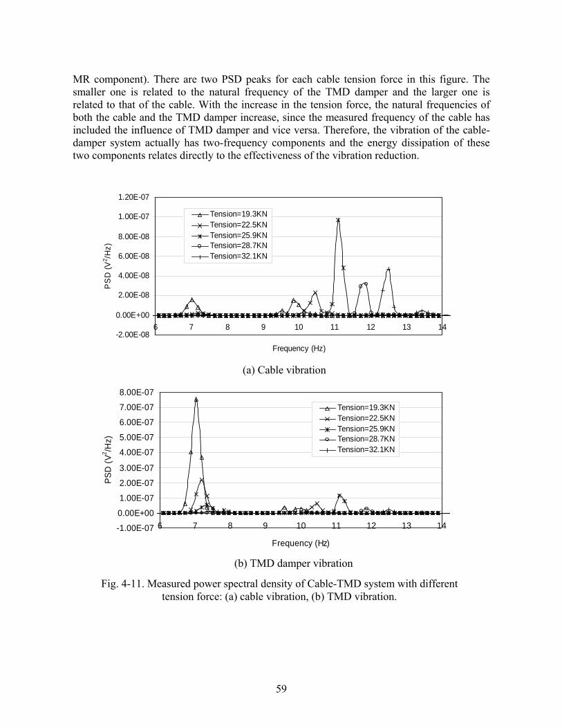
MR component). There are two PSD peaks for each cable tension force in this figure. The smaller one is related to the natural frequency of the TMD damper and the larger one is related to that of the cable. With the increase in the tension force, the natural frequencies of both the cable and the TMD damper increase, since the measured frequency of the cable has included the influence of TMD damper and vice versa. Therefore, the vibration of the cable-damper system actually has two-frequency components and the energy dissipation of these two components relates directly to the effectiveness of the vibration reduction.

Fig. 4-11. Measured power spectral density of Cable-TMD system with different tension force: (a) cable vibration, (b) TMD vibration.

(a) Cable vibration

-2.00E-08

0.00E+00

2.00E-08

4.00E-08

6.00E-08

8.00E-08

1.00E-07

1.20E-07

6 7 8 9 10 11 12 13 14

Frequency (Hz)

PS

D (V

2 /Hz)

Tension=19.3KNTension=22.5KNTension=25.9KNTension=28.7KNTension=32.1KN

(b) TMD damper vibration

-1.00E-07

0.00E+00

1.00E-07

2.00E-07

3.00E-07

4.00E-07

5.00E-07

6.00E-07

7.00E-07

8.00E-07

6 7 8 9 10 11 12 13 14

Frequency (Hz)

PSD

(V2 /H

z)

Tension=19.3KNTension=22.5KNTension=25.9KNTension=28.7KNTension=32.1KN

59

In Fig. 4-11(a), the vibration energy of the cable centralizes mainly around the natural frequency of the cable (e.g., about 11.0Hz with a tension force of 25.9kN), and the energy corresponding to the TMD damper natural frequency (about 7.0Hz) is very small. However, as shown in Fig. 4-11(b), the vibration energy of the damper is dominated by the natural frequency of the TMD damper (about 7.0Hz), and the energy corresponding to the cable natural frequency (about 11.0Hz) is significantly less. This means that the energy of the combined system has transferred from the cable to the TMD damper.

In addition, adding dampers to the cable will affect the cable natural frequency. Main

and Jones (2002) had a discussion about the cable frequency shift due to the supplemental viscous damper that was anchored to the deck. According to the present experimental results, adding the TMD-MR damper or TMD damper also affects the cable natural frequency. From Table 4-5, we can see that by adding the TMD damper, the frequency of the cable-TMD system is less than that of the pure cable, though the frequency shift is small.

Table 4-5. Frequency shift of cable-TMD system

Cable Tension (kN) 19.3 22.5 25.9 28.7 32.1 Frequency of pure cable

(Hz) 10.16 10.94 11.72 12.5 13.13

Frequency of cable-TMD (Hz) 9.84 10.47 11.09 11.88 12.5

4.7 Factors Affecting Vibration Reduction Effectiveness

As stated earlier, adding the TMD-MR damper to the cable not only improves the

cable damping, but also changes the natural frequency of the cable system. This change may affect the dynamic response of the cable-TMD-MR system to a forced vibration. Fig. 4-12 plots the maximum acceleration response to a sinusoidal excitation with different cable experimental setups. For the convenience of discussion, Table 4-6 defines the experimental setups and the corresponding case numbers that are shown on the x-axis in Fig. 4-12. It is noted that after the addition of the MR damper, the natural frequency of the TMD-MR damper system (about 8 Hz) is different from that of the TMD component only system (about 7Hz).

The curves in Fig. 4-12 can be classified into 3 categories with different ranges of excitation frequencies. When the excitation frequency equals 5Hz or 6Hz, which is away from the natural frequency of both the cable (about 9Hz that is related to a cable tension force as shown in Fig. 4-6) and the TMD-MR damper (about 8Hz), the best vibration reduction happens in the case of the passive TMD-MR system (with 0A current, Case 3) for both the cable vibration and the TMD-MR vibration. With the current inside the MR damper increasing from 0A to 0.05A, the cable vibration increases and remains almost the same when the current changes from 0.05A to 0.20A. This phenomenon is called the saturation effect of MR dampers, which implies that a larger current in the MR damper does not guarantee a better effectiveness of cable vibration control.

60

Fig. 4-12. Measured maximum acceleration of cable-TMD-MR system under different experiment setup: (a) cable vibration, (b) TMD-MR damper vibration.

(a) Cable vibration

0

0.002

0.004

0.006

0.008

0.01

0.012

0.014

0.016

0.018

0 1 2 3 4 5 6 7 8

Different Vibration Cases

Max

Acc

(V)

f=5Hzf=6Hzf=7Hzf=8Hzf=9Hzf=10Hz

(b) TMD-MR damper vibration

0

0.002

0.004

0.006

0.008

0.01

0.012

0.014

0.016

0.018

0 1 2 3 4 5 6 7 8

Different Vibration Cases

Max

Acc

(V)

f=5Hzf=6Hzf=7Hzf=8Hzf=9Hzf=10Hz

The following reasons may help explain why the vibration increases when the current increases from 0A to 0.05A. Firstly, when the excitation frequency is away from the cable frequency and the TMD-MR system frequency, the cable vibration is small so that the control effectiveness of the TMD-MR system is also small since the dissipation function of the MR component is not fully activated. Secondly, a larger current in the MR damper will cause a shift of the natural frequency of the TMD-MR system, which may counteract the beneficial vibration reduction effect due to its increase in damping.

61

When the excitation frequency reaches 7Hz, which is close to the TMD frequency, a significant damper vibration is observed in Fig. 4-12(b) for Case 2. When the excitation frequency reaches 8Hz, the most noticeable reduction of cable vibration is the TMD component only case (see Case 2 in Fig. 4-12 (a)). Both the cable and the TMD vibrations of Case 2 are less than that of the passive TMD-MR case (Case 3). With this excitation frequency, the cable vibration increases slightly with the increase in the MR damper current until the current reaches 0.15A (Case 6). The TMD-MR damper vibration reduces when the current changes from 0A (Case 3) to 0.10A (Case 5) and increases slightly when the current changes from 0.10A (Case 5) to 0.20A (Case 7).

In all the above cases, the excitation frequency is away from the cable natural

frequency so that the cable vibration is relatively small, even if no damper is provided. When the excitation frequency reaches 9Hz or 10Hz, as shown in Fig. 4-12(a), the cable vibration without damper is about 1 to 2-order larger than that with the excitation frequency being away from the cable natural frequency (such as 5 to 7 Hz). The effectiveness of the TMD-MR damper becomes obvious in these resonant vibration cases. The vibration of the cable for the TMD-MR damper with 0A current case (Case 3) is close to that of TMD only case (Case 2) and much smaller than that of pure cable vibration without dampers (Case 1). An increase in the current from 0A (Case 3) to 0.05A (Case 4) leads to a smaller cable vibration, from 0.05A (Case 4) to 0.10A (Case 5) leads to a slightly larger cable vibration, and from 0.10A (Case 5) to 0.20A (Case 7) leads to almost the same cable vibration. Comparing these observations of 9Hz and 10Hz cases with those of 5Hz and 6Hz cases, it can be seen that the current in the MR damper corresponding to the best vibration reduction effectiveness changes from 0A to 0.05A, and the current corresponding to the beginning of saturation increases from 0.05A to 0.10A. This observation shows that the TMD-MR damper system is more suitable for reducing large cable vibrations that can activate the shaft movement of the MR damper.

Table 4-6. Case definitions of experimental setup for Fig. 4-12

Case Number 1 2 3 4 5 6 7

Experiment Cases

No damper

TMD only

Passive TMD-MR

a = 0A

TMD-MR

a=0.05A*

TMD-MR

a=0.10A

TMD-MR

a=0.15A

TMD-MR

a=0.20A * Meaning that the TMD-MR damper system is attached to cable with a current of 0.05A (typical). 4.8 Summary of Observed Phenomena and Control Strategies

It has been observed that the relationship among the natural frequencies of the cable,

the TMD-MR damper system, and the excitation forces will affect the cable response significantly. When the excitation frequency is away from that of the cable and the TMD-MR damper, the cable vibration is not significant and the TMD-MR damper reduces the cable vibration, mainly depending on the MR component with two effects – providing additional damping and stiffness. When the MR component is in its passive mode, it provides additional

62

damping and very small additional stiffness. However, when the current in the MR component increases, the stiffness as well as the natural frequency of the TMD-MR damper change; and the shaft movement of the MR damper tends to be locked, which will also affect the cable natural frequency. These factors may be detrimental to the vibration control, as it is observed that the cable vibration reduction effectiveness becomes worse with an increased current in Fig. 4-12. Therefore, when the vibration is small, the MR component should be set to its passive mode.

When the excitation frequency is close to that of the TMD-MR damper system while it

is still away from the cable frequency, the cable vibration will be damped out mainly due to the MR component. However, whether the vibration of the TMD-MR damper should be large or small may still be hard to identify because of the following reasons. On one hand, the vibration of the TMD-MR damper would be large because it absorbs the cable vibration energy, while on the other hand, the vibration of TMD-MR system would be small because the MR component can dissipate energy. The actual vibration of the TMD-MR damper depends on the relative importance of these two effects.

When the excitation frequency is close to the cable’s natural frequency, both the TMD

component and the MR component of the TMD-MR damper can work efficiently so that the vibrations of both the cable and the TMD-MR system are reduced. In this case, the TMD-MR damper should be in its active mode with a developed control strategy to adjust the current.

A good vibration control strategy also needs to be decided regarding how to optimally

utilize the two components of the TMD-MR damper, namely the TMD and MR components. It is common sense that for an efficient vibration control, the natural frequency of the TMD-MR system should be tuned to the natural frequency of the cable-damper system, which has been verified by the observed experimental results. As a result, when the excitation frequency is away from the cable natural frequency, the cable vibration will not be serious and the MR component with a small current will be enough to reduce the vibration. A large current in the MR component may lock the movement of the MR component and thus deteriorate the damping effectiveness.

When the excitation frequency is close to the cable natural frequency as well as the

TMD-MR damper natural frequency, the TMD component of the TMD-MR damper will transfer a large amount of vibrations from the cable to the TMD-MR damper, and the vibrations will be dissipated by the MR component with a relatively larger current. This is the ideal situation for TMD-MR applications. However, in practical situations, an exact match of the natural frequency between the TMD-MR damper and the cable system is hard to achieve because the cable natural frequency may change due to various reasons such as deterioration. Also, when the excitation has a wide frequency range, the TMD component cannot be as efficient for such a wide frequency range. In these cases, the MR component is counted on for helping to tune the TMD-MR natural frequency to track the dominant excitation frequency. Theoretical guidance is needed to design an optimal TMD-MR system with a good balance between the TMD and MR components.

63

4.9 Conclusions This study presents a novel hung-on TMD-MR damper system for cable vibration

control. The developed TMD-MR damper absorbs the cable vibration energy through both the TMD component and the MR component. Experimental study was conducted to verify the concept and to understand the performance of the cable-TMD-MR system.

It was observed that the cable resonant vibration was considerably reduced down to

20%~30% of the cable vibration without the dampers. In addition, the installation of the TMD-MR damper system changed the dynamic characteristics of the cable, such as its natural frequency, so that the reduction effectiveness of the TMD-MR system on the cable vibration varied with different excitation frequencies. Based on the experimental observations, when the natural frequency of the TMD-MR damper system was tuned close to that of the cable, good vibration reduction efficiency was achieved. However, optimal tuning to achieve the best vibration reduction is not straightforward due to the interaction between the cable and the damper, as discussed in the companion study (Wu and Cai 2006). After the optimal tuning process is achieved, the TMD-MR damper system is expected to be more effective for a wider range of different excitation frequencies than a traditional TMD.

When the excitation frequency is away from the cable natural frequency, the MR

component contributed mainly in providing an additional damping, and the TMD-MR should be set in the passive mode. In these small vibration cases the cable vibration is too small to activate the MR damper movement. Therefore, a large current in the MR damper will tend to lock the MR damper’s shaft movement and thus deteriorate the damping effectiveness.

When the excitation frequency is close to the cable natural frequency, the cable

vibration became large. At this time, the TMD component contributed mainly to track the excitation frequency and transfer vibration energy to the damper and the MR component worked as an energy dissipater to help reduce the cable vibration. The addition of the MR damper makes the TMD-MR damper system adaptable.

Now that the concept of the TMD-MR system has been verified through experimental

observations, theoretical guidance is needed for a more rational design of the TMD-MR damper. This work is in progress by the writers, and part of the work is presented in the companion study (Wu and Cai 2006). 4.10 References Angelo, W.J. (1997). “Lasers Ensure Stay Cable Safety.” Engineering News-Record, July 28.

pp.10. Cai, C. S. and Wu, W. J. (2004) “Development of an Adaptive Damper for Cable Vibration

Control.” A Final Report, Project No. NCHRP-92, submitted to the IDEA Program, Transportation Research Board, National Research Council, Louisiana State University, Baton Rouge, Louisiana.

64

Caracoglia, L., and Jones, N. P. (2002) “Analytical method for the dynamic analysis of complex cable structures.” Proceeding, ASCE Engineering Mechanics Division Conference, Columbia University, NY.

Chen, Z.Q., Wang, X. Y., Ko, J. M., Ni, Y.Q., Spencer, B.F., and Yang, G. Q. (2003). "MR

damping system on Dongting Lake cable-stayed bridge." Smart Systems and Nondestructive Evaluation for Civil Infrastructures, San Diego, California, USA, 2-6 March 2003, pp.229-235

Christenson, R. E., Spencer, B. F. Jr. and Johnson, E. A. (2002). "Experimental Studies on the

Smart Damping of Stay Cables." Proc. of 2002 ASCE Structures Congress, Denver, Colorado, USA. April.

Ciolko, A.T., and Yen, W. P. (1999). “An immediate Payoff from FHWA’s NDE Initiative.”

Public Roads, May/June, 10-17. Dyke, S.J., Spencer, B.F., Jr., Sain, M.K., and Carlson J.D. (1996a). “Seismic Response

Reduction Using Magnetorheological Dampers.” Proc. of IFAC World Congress, San Francisco, CA, Vol. L, 145-150.

Dyke, S.J., Spencer, B.F., Sain, M.K., and Carlson, J.D. (1996b). “Modeling and Control of

Magnetorheological Dampers for Seismic Response Reduction.” Smart Materials and Structures, 5, 565-575.

Flamand, O. (1995). “Rain-wind induced vibration of cables.” Journal of Wind Engineering

and Industrial Aerodynamics, 57, 353-362. Irvine, H.M. (1981) “Cable Structures.” The MIT press. Johnson, E. A., Christenson, R. E., and Spencer, B. F. (2003). "Semiactive damping of cables

with sag." Computer-Aided Civil and Infrastructure Engineering, 18, 132-146. Langsoe, H. E., and Larsen, O. D. (1987). “Generating Mechanisms for Cable Stay

Oscillations at the FARO Bridges.” Proc. of Int. Conf. on Cable-stayed Bridges, Bangkok, Nov. 18-20.

Lord Corporation (1999) “Engineering Note for Designing with MR Fluids”

http://literature.lord.com/root/other/rheonetic/designing_with_MR_fluids.pdf Lord Corporation. (2004). http://www.lord.com/Default.aspx?tabid=1127&page=1&docid

=684.

65

Lou, W. J., Ni, Y. Q., and Ko, J. M. (2000). "Dynamic Properties of a Stay Cable Incorporated with Magnetorheological Fluid Dampers." Advances in Structural Dynamics, J.M. Ko and Y.L. Xu (eds.), Elsevier Science Ltd., Oxford, UK, Vol. II, 1341-1348.

Main, J. A., and, Jones, N. P. (2001). "Stay-cable vibration in cable-stayed bridges:

Characterization from full-scale measurements and mitigating strategies." Journal of Bridge Engineering, 6(6), 375-387.

Main, J. A., and, Jones, N. P. (2002). "Free vibration of taut cable with attached damper. I:

linear viscous damper." Journal of Engineering Mechanics, 128(10), 1062-1071. Phelan, R. S., Mehta, K. C., Sarkar, P.P. and Chen, L. (2002). “Investigation of Wind-Rain-

Induced Cable-Stay Vibrations on Cable-Stayed Bridges” Final Report, Center for Multidisciplinary Research in Transportation, Texas Tech University, Lubbock, Texas.

Spencer, Jr., B. F., Carlson, J. D., Sain, M. K., and Yang, G. (1997a). "On the current status of

magnetorheological dampers: Seismic protection of full-scale structures." Proceedings of American Control Conference, 458–462.

Spencer, B.F., Dyke, S.J. Sain, M.K. and Carlson, J.D. (1997b) "Phenomenological model of

a magnetorheological damper." Journal of Engineering Mechanics, Vol. 123, No. 3, 230-238

Tabatabai, H., Mehrabi, A.B., Morgan, B.J., and Lotfi, H.R.. (1998). “Non-destructive Bridge

Evaluation Technology: Bridge Stay Cable Condition Assessment.” Final report submitted to the FHWA, Construction Technology Laboratories, Inc., Skokie, IL.

Tabatabai, H., and Mehrabi, A. B. (1999). “Tuned Dampers and Cable Fillers for Suppression

of Bridge Stay Cable Vibrations.” Final report to TRB IDEA program, Construction Technology Laboratories, Inc, Skokie, Illinois.

Tabatabai, H., and Mehrabi, A. B. (2000). “Design of Mechanical Viscous Dampers for Stay

Cables.” Journal of Bridge Engineering, 5(2), 114-123. Wu, W. J. and Cai, C. S. (2006). “Cable vibration control with a TMD-MR damper system:

Theoretical formulation and parametric study” Journal of Engineering Structures, (submitted)

Xu, Y. L., Yu, Z. and Ko, J. M. (1997). “Forced vibration studies of sagged cables with oil

damper using a hybrid method.” Engineering Structures, Vol. 20(8), 692-705.

66

CHAPTER 5 THEORETICAL EXPLORATION OF A CABLE AND A TMD SYSTEM 5. 1 Introduction

As key load carrying members for cable-stayed bridges, stay cables are of primary

importance to secure the safety of the entire structure. Since cables are generally flexible, relatively light and low energy-dissipative because of their intrinsic low damping, they are susceptible to external disturbances such as wind, wind-rain, earthquake, and traffic induced loadings. To suppress the problematic vibrations, mechanical dampers, with one end connected to the cable and the other end to the deck near the anchorages of the cables, have been studied (Yamaguchi and Fujino 1998). Though the attached dampers have been demonstrated effective in some applications in reducing the cable vibrations, they are not most effective because they are restricted to the cable ends. TMD dampers that can be placed anywhere along the cables overcome the shortcomings of traditional mechanical dampers (Tabatabai and Mehrabi 1999). However, the frequency sensitivity of the control efficiency makes TMDs difficult to be implemented. A newly proposed TMD-MR (Tuned Mass Damper-Magnetorheological) damper system in the companion study (Cai et al. 2006) is a promising way to combine the position flexibility of the TMD and the adjustability of the MR damper. It has experimentally been demonstrated effective in cable vibration reduction (Cai and Wu 2004, Cai et al. 2006). The potential for actual applications of the TMD-MR damper system for cable vibration reduction necessitates a thorough understanding of the resulted cable-damper dynamic system, and a numerical procedure for a rational TMD-MR damper design, both of which are not available in the literature.

Since the first half of the eighteenth century, many researchers have shown their

interests in cable vibration problems (Starossek 1994). Irvine and his collaborators (Irvine and Caughey 1974, Irvine 1976, Irvine 1981) developed a theory after they performed an extensive research on different rigidly supported cable profiles including both horizontal and inclined configurations for both free and forced vibrations.

Carne (1981) was one of the first to study the vibrations of a taut cable with an

attached damper. He developed an approximate analytical solution by obtaining a transcendental equation for the complex eigenvalues and an approximation for the first-mode damping ratio as a function of the damper coefficient and location. Pacheco et al. (1993) formulated a free-vibration problem through Galerkin’s approach by using sinusoidal mode shapes of an undamped cable as basis functions. Several hundred terms were required for an adequate convergence of the solution, creating a computational burden. They also introduced nondimensional parameters to develop a “universal estimation curve” of normalized modal damping ratio versus normalized damper damping coefficient, which is useful and applicable in many practical design situations. Krenk and his collaborators (2000 and 2002) developed an analytical solution of a free-vibration problem for a cable and, by using an iterative method, obtained an asymptotic approximation for the damping ratios for all modes for damper locations near the end of the cable. Main and Jones (2002) similarly discussed a horizontal cable with a linear viscous damper, using analytical formulations of a complex eigenvalue problem. They discussed the theoretical solutions and the physical situations that

67

those solutions represent. In addition, they pointed out the importance of damper-induced frequency shifts in characterizing the response of the cable-damper system. Johnson et al. (2003) discussed the performance of a general cable-semiactive damper system. In general, the dynamics of cable-viscous damper (anchored to deck) systems have been well investigated by previous researchers.

Since the TMD-MR damper system is a new development in cable vibration reduction,

the primary goal of this study is to investigate the cable-TMD-MR system theoretically to obtain a more profound and extended understanding of the system performance. An analytical formulation of a free-vibration problem was conducted to investigate the dynamic characteristics of the cable-TMD-MR damper system. The change of the dynamic characteristics affected by the system parameters, such as the position of the damper, the mass and frequency ratios between the damper and the cable, and the damping ratio of the damper, was studied thoroughly. This parametric study provides necessary insights into the system dynamics in order to rationally design the cable-TMD-MR system.

5.2 Problem Statement and Analytical Solution

The prototype cable-TMD-MR system under consideration (Cai et al. 2006) is simulated here with a taut horizontal cable and a damper as shown in Fig. 5-1 where the TMD-MR damper in the vertical vibration is modeled as an equivalent system consisting of a spring K and a dashpot with a damping coefficient , and a mass C M . The damping coefficient represents the equivalent damping of the MR component and can be obtained by a linearization process (Li et al. 2000). Therefore, in the present study, the terminologies of TMD and TMD-MR are exchangeable hereafter. According to Irvine (1978), the result obtained from a cable with a horizontal configuration can be readily transformed to an inclined configuration. Therefore,, the horizontal cable configuration is chosen for the current study for simplicity. In this calculation model, a spring-dashpot-mass system representing the TMD-MR damper is attached to the cable at an intermediate point, dividing the cable into two segments. Without losing generality, it is assumed that . In addition, the following assumptions are made:

C

12 ll >

1) The tension force in the cable is large compared to its weight so that the vertical sag is small. 2) The bending stiffness and intrinsic damping of the cable is small. 3) The cable deflection is small so that the secondary tension force caused by the deflection is neglected.

T T

MK C

l1 l2

x1 x2

Fig. 5-1. Calculation model for the cable-TMD-MR system.

68

With these conditions, the following partial differential equation is satisfied over each segment of the cable:

2

2

2

2 ),(),(t

txvmx

txvT kk

k

kk

∂∂

=∂

∂ (5-1)

where T is the axial tension force in the cable; is the mass per unit length; is the coordinate along the cable of the k -th segment with the origin at the cable end; and is the transverse deflection. A nondimensional time parameter

m kxv

tcωτ = is introduced to simplify the

expression, and mTLc /)/(πω = is the fundamental natural frequency of the cable. Traditionally, the variable separation method is used to solve Eq. (5-1) where the

solution of the cable is assumed to have the following form, (5-2) ττ s

kkkk exVxv )(),( =where is a dimensionless eigenvalue that is complex in general, and is the mode shape of cable vibration. Substituting Eq. (5-2) into Eq. (5-1) yields the following ordinary differential equation,

s kV

kk

kk VLs

dxxVd 2

2

2

)()( π= (5-3)

From the fixed end boundary conditions, we have,

0),0( =τkv , 2,1=k (5-4) The continuity of the cable at the conjunction point of the two segments requires,

)(),(),( 2211 τγττ == lvlv (5-5) where γ is the displacement of the conjunction point in terms of time.

With these boundary and continuity conditions, the cable displacement can be expressed as,

)/sinh()/sinh()(),(

LslLsxxv

k

kkk π

πτγτ = (5-6)

Considering the vertical equilibrium condition of the cable at the attachment point of

the damper, we have,

)()()(11

11

2211

11

2

2

1

1

dtdv

dtdvCvvK

xv

xvT d

lxdlx

lxlx

−+−=∂∂

−∂∂

−=

=

==

(5-7)

where is the vertical displacement of the damper. dv Meanwhile, from the equilibrium of the TMD-MR damper system itself, we have,

0)()( 2

21

111

11=−−+−

== dt

vdMdt

dvdtdvCvvK dd

lxdlx

(5-8)

69

For each vibration mode of the combined cable-damper system, the damper has the same vibration pattern (i.e., the same time function) as the cable at the attachment point so that the displacement of the damper system can be expressed as, )(τβγ=dv (5-9) where β is the complex amplitude ratio between the damper and the corresponding cable point, which can be determined by each solution of . s

By denoting and 2

dMK ω= ξωdMC 2= , we can derive β from Eq. (5-8) as,

222121

sssρξρ

ξρβ++

+= (5-10)

where dω and ξ are the natural frequency and the damping ratio of the damper, respectively,

and d

c

ωωρ = is the ratio between the cable fundamental vibration frequency and the damper

vibration frequency, which is referred as frequency ratio hereafter. When the frequency ratio i/1=ρ , , it is called i -th mode tuning in this study. 1,2,i = Ln

Substituting Eq. (5-10) into Eq. (5-7), we have,

021

21)coth()coth( 2221 =

+++

++ss

smM

Ls

Lsl

Lsl

ρξρξρπππ (5-11)

Eq. (5-11) is referred as the basic complex equation hereafter, which can be solved

numerically. Its roots are the eigenvalues of the combined cable-damper system. Usually, the complex value can be expressed as the sum of its real and imaginary

parts as, s

iii js ϕσ += (5-12)

If we denote )( ic

ii ζ

ωωσ −= and )1( 2

ic

ii ζ

ωωϕ −= , then ciii ωϕσω 22 += and

)2/1(2

2

)1( −+=i

ii σ

ϕζ are the corresponding i-th system modal frequency and damping,

respectively. 1−=j is the imaginary root. iω has been referred as the pseudo-undamped natural frequency (Pacheco et al. 1993). Therefore, iϕ can be referred as the i-th normalized damped frequency. In the following, a denotation without subscript represents any mode in general.

Substituting Eq. (5-12) into Eq. (5-11) and separating the equation into the real and

imaginary parts, we can obtain the real part equation as,

70

0))22()21(

)2()4()2()22()21(

)4()4()4((

)/2cos()/2cosh()/2sinh(

)/2cos()/2cosh()/2sinh(

2222222

3432234

2222222

22222223222

2

11

1

=++−++

++

+++−++

+++++

+−

+−

ϕσρξρϕϕρσρξρσξρϕξρσϕξρσ

ϕσρξρϕϕρσρξρσρξρσϕρξρσξρσσπ

πϕπσπσ

πϕπσπσ

LmM

LlLlLl

LlLlLl

(5-13)

and the imaginary part equation as,

0))22()21(

)4()4()22()21(

)44()4((

))/2cos()/2))(cosh(/2cos()/2(cosh()2sin(2)/2cosh()/2sin(2)/2cosh()/2sin(2

2222222

222322222

2222222

332211

2211

=++−++−+−

+++−++

−++

+−−

+−−

ϕσρξρϕϕρσρξρσρρξϕρρξσϕ

ϕσρξρϕϕρσρξρσξρξρϕσξρϕσϕπ

πϕπσπϕπσπϕπσπϕπσπϕ

LmM

LlLlLlLlLlLlLlLl

(5-14)

These two equations are similar to those of Main and Jones (2002), which discussed

the cable with ground-anchored viscous damper system. Eqs. (5-13) and (5-14) are very complicated due to the introduction of the TMD-MR damper system, which makes a general analytical simplification very difficult and a numerical solution is thus pursued in the present study.

Meanwhile, from Eq. (5-6), the complex mode shape can be expanded explicitly in terms of the real and imaginary parts of , yielding the following expression, s )]/sin()/cosh()/cos()/[sinh()( LxLxjLxLxAxV kkkkkkk πϕπσπϕπσ += (5-15) where is a complex coefficient. ))//(sinh()( τπτγ s

kk eLslA = Generally, if parameters of the cable-damper system are specified, there are an infinite

number of complex values satisfying Eq. (5-11) corresponding to different modes. The addition of the damper to the cable actually increases by one more degree of freedom to the cable, making the dynamics of the combined cable-damper system much different from the original pure cable system. The solution corresponding to the added degree of freedom is close to that of a particular vibration mode that the damper is tuned to. Therefore, if a damper is tuned to the i -th mode of the cable, there are two solutions of s for the cable-damper system, both of which are close to the corresponding -th solution of the pure cable. For the convenience of the narrative, the added solution and the corresponding mode of the combined cable-damper system will be marked with a subscript “2” in the following discussion since it reflects more about the damper related vibration, though it does affect the dynamic properties of the combined system. Correspondingly, the mode shape and the amplitude ratio

s

i

)( kk xV β are complex values associated with each solution of . s

71

The values of iσ and iϕ determine the vibration characteristics of the cable-damper system. It can be observed from Eq. (5-2) that, when 0=iϕ or pure imaginary value, the displacement for each point along the cable becomes a pure hyperbolic function of time, which means that the cable vibration will decay without oscillation. In this case, iζ is larger than or equal to its critical value 1.0, representing an overdamped system. When 0=iσ , the cable displacement becomes a pure trigonometric function of time; correspondingly, the system damping iζ becomes zero, which means that the cable will vibrate in a manner of nondecaying oscillation, representing an undamped system. More detailed discussions of these two special cases will be given in the following sections. 5.3 Special Case of Nonoscillatory Decaying Vibration

When the solution of Eqs. (5-13) and (5-14) is a purely real number, it corresponds

to a nonoscillatory, exponentially decaying vibration since the displacement term in Eq. (5-2) becomes a hyperbolic function of time. In this case, the imaginary part

s

0=iϕ or iϕ becomes a pure imaginary value ( 1=iζ or 1>iζ accordingly). In the following derivation, 0=iϕ is assumed. (For iϕ with a pure imaginary value and 1>iζ , a similar derivation can be performed directly from the basic complex equation, Eq. (5-11).) As a result, Eq. (5-14) is trivially satisfied, while Eq. (5-13) becomes, 0

)21()21(

)/coth()/coth( 2221 =++

+++

ii

iiii Lm

MLlLlσρξρσ

ξρσσππσπσ (5-16)

To satisfy Eq. (5-16), the iσ value should be negative. The number of negative real

solutions of this equation depends on the relationship of the parameters. For each ρ , negative solutions exist only when the damping ratio ξ exceeds a threshold value. This indicates that if the natural frequency of TMD-MR damper is given, only when its damping reaches some threshold value, the free vibration of the cable-damper system begins to decay without oscillation. Correspondingly, the system modal damping is larger than or equal to 1.

For example, assume that the damper is placed at the mid-span of the cable with its

frequency tuned to the fundamental natural frequency of the cable ( ρ = 1), and the mass ratio is 5%. In this case, Eq. (5-16) reduces to, 0

)21()21(05.0)5.0coth(2 2 =

+++

+ii

iii σξσ

ξσσππσ (5-17)

Fig. 5-2 shows the dependence of the number of the solutions on the value of the

damping ratio ξ of the damper. In this figure, )5.0coth(21 iy πσ= ,

)21()21(05.0 22ii

iiyσξσ

ξσσπ++

+−= and the intersection points between y1 and y2 represent the

solution points of Eq. (5-17). The threshold damping ratio of the damper in this case is about 0.963. When the damping ratio is less than the threshold value 0.963, only complex solutions

72

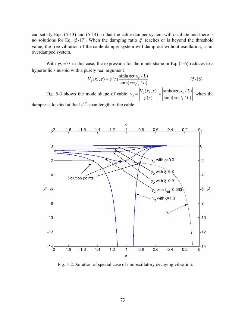
can satisfy Eqs. (5-13) and (5-14) so that the cable-damper system will oscillate and there is no solutions for Eq. (5-17). When the damping ratio ξ reaches or is beyond the threshold value, the free vibration of the cable-damper system will damp out without oscillation, as an overdamped system.

With 0=iϕ in this case, the expression for the mode shape in Eq. (5-6) reduces to a

hyperbolic sinusoid with a purely real argument

)/sinh()/sinh()(),(

LlLxxV

ki

kikk πσ

πστγτ = (5-18)

Fig. 5-3 shows the mode shape of cable )/sinh()/sinh(

)(),(

3 LlLxxVy

ki

kikk

πσπσ

τγτ

== when the

damper is located at the 1/4th span length of the cable.

Fig. 5-2. Solution of special case of nonoscillatory decaying vibration.

73

Fig. 5-3. Mode shape associated with purely real eigenvalue.

5.4 Special Case of Nondecaying Oscillation When the solution is purely imaginary (i.e.,s 0=iσ and 0=iζ ), it corresponds to a

nondecaying oscillation or zero damping vibration. The displacement term of Eq. (5-2) becomes a pure trigonometric function of time. Under this condition, the basic complex equation of motion, Eq. (5-11), becomes,

0))(21(

)21()/coth()/coth( 2221 =++

+++

ii

iiii jj

jjLmMLljLlj

ϕρϕξρϕξρϕπϕπϕπ (5-19)

To ensure both the real and imaginary parts to be equal to zero, Eq. (5-19) leads to,

0)2()1(

22222

43

=+− ii

i

LmM

ξρϕϕρϕξρπ (5-20)

0)2()1(

4))cot()(cot(2222

3223221 =

+−+−

++−ii

iiiii

LmM

Ll

Ll

ξρϕϕρϕρξϕρϕππϕπϕ (5-21)

74

To satisfy Eq. (5-20), either iϕ should be zero, or the damping ratio ξ should approach zero or infinity. Obviously, 0=iϕ is not a solution since it cannot satisfy Eq. (5-21). For each limit value ξ (zero or infinity), there is one set of frequencies iϕ satisfying Eq. (5-21) accordingly. One set of frequencies is associated with the limit of 0→ξ , which physically means that no damping is provided by the damper (there is no MR component); the other set is associated with the limit of ∞→ξ , which physically means that the MR damper works as a rigid bar (MR component is too strong). Both of these two limit cases correspond to a zero system damping, which indicates that there should be an optimal damping for the TMD. This observation is similar to that of the cable-viscous damper system (Main and Jones 2002).

In the first extreme case, i.e., when 0→ξ , Eq. (5-21) reduces to,

0)1(

))cot()(cot( 2221 =

−++−

i

iii

LmM

Ll

Ll

ϕρϕππϕπϕ (5-22)

For each parameter set, there are different iϕ values that can satisfy this equation. For

example, when , Ll 5.01 = 05.0=LmM , 1=ρ , Eq. (5-22) becomes,

0)1(

05.0)5.0cot(2 2 =−

+−ϕ

ϕππϕ (5-23)

For the case of the first mode tuning, there are two solutions of the cable-damper

system that are close to that of the first mode of the pure cable vibration, , (5-24) 849901

1.=ϕ 1621.12

1=ϕ

In the second extreme case, i.e., when ∞→ξ , Eq. (5-21) reduces to,

0))cot()(cot( 21 =++− iii

LmM

Ll

Ll ϕππϕπϕ (5-25)

Also by choosing , Ll 5.01 = 05.0=LmM , 1=ρ , this equation becomes,

005.0)5.0cot(2 =+− ii πϕπϕ (5-26) In this case, just one solution 95240.=ϕ is obtained for the first mode since

physically the damper is a rigidly connected mass to the cable so that the damper does not add an extra degree of freedom to the system.

Under the first extreme case with 0→ξ , the mode shape Eq. (5-15) reduces to, )]/sin([)( LxjAxV kikkk πϕ= (5-27)

75

Usually, one of the two solutions of ϕ for the first mode is larger than 1.0, which means that the mode shape is part of a sine wave for the whole cable length, and the other is less than 1.0, which means that the mode shape consists of more than one sine wave. The resultant system modal vibration is a combination of these two mode shapes. 5.5 Numerical Parametric Study

Parameters such as the location, stiffness, and damping of the damper will affect the

free vibration response of the cable-damper system. The system modal damping is focused in this study, since it reflects directly the vibration control efficiency.

Since Eqs. (5-13) and (5-14) are very complicated, numerical calculations are

conducted here to investigate and understand the effect of different parameters on the system dynamics. In this analysis, a basic set of parameters has been chosen as a base for varying those parameters. The criteria for the selection of the basic parameter set are, (a) close to the experimental setup that was used in the companion study (Cai et al. 2006), such as the cable length and the tension force, though not exactly the same; (b) based on practical experience, such as the commonly used mass ratio and the frequency ratio of TMDs; (c) reasonable parameter range, such as the damping coefficient of the damper. However, to take into consideration of some special conditions, a few theoretically important values are also discussed, such as the MR damping ratio that is larger than 1.0. Based on the basic parameter set, more parameter sets are chosen by varying one or more parameters around the basic one. The basic parameters and their variation ranges are listed in Table 5-1. The cable length and the tension force are not listed since their effects are included in the parameters of the mass ratio and the frequency ratio. When all the parameters are specified, the nondimensional complex eigenvalue can be readily solved by numerical iterations. s

Table 5-1. Basic parameter set and the parameter variation range*

Ll /1 0/ KK ** )/(LmM ξ ρ Basic Parameter

Set 0.5 1 0.05 0.1 1

Parameter Variation Range 0.05~0.5, 0.01~100 0.01~0.20 0.01~2 0.1~10

*: The variation range may change slightly in some discussions. **: is determined by other parameters as basic TMD-MR mass and cable fundamental frequency.

0K

5.5.1 Effect of TMD-MR Position on System Damping

Fig. 5-4 shows the system modal damping of the first four modes versus the position

change of the damper. The other parameters are the basic values given in Table 5-1 and the damper is tuned to the first cable vibration mode ( 1=ρ ). Since there are two modes in the neighborhood of the first mode of the pure cable because the damper is tuned to the first

76

mode, the mode associated with the cable is marked as “mode 1, 1” and the other mode associated with the damper is marked as “mode 1, 2”. For the convenience of narrative, the modal damping associated with “mode 1, 1” is called the first modal damping hereafter since the “mode 1, 1” is more cable vibration related. The modal damping corresponding to “mode 1, 2” deceases when the damper moves from the end towards the mid-span, while the fist modal damping increases correspondingly, which implies that the modal damping will transfer from the damper related mode to the cable related mode as the damper moves towards the mid-span. More attention will be paid to the cable related modal damping thereafter so that just the corresponding mode associated with the cable will be discussed.

The first modal damping increases significantly before the damper reaches the 1/10th point of the cable length. However, the increase rate slows down after it passes this point. When the damper reaches the mid-span of the cable, the first modal damping reaches its’ maximum value of 6.27%. Usually, when a viscous damper is connected one end to the cable and the other end to the deck, the maximum system modal damping is about 1.0% when the damper is installed at 2% of the cable length and 2.5% when the damper is placed at 5% of the cable length (Main and Jones 2002), which is almost the upper limit installation position for a long stay cable.

Fig. 5-4. Effect of TMD-MR damper position on system damping.

0.000.010.020.030.040.050.060.070.080.090.10

0.00 0.10 0.20 0.30 0.40 0.50

l 1/L

ζ

Mode 1,2Mode 1,1Mode 2Mode 3Mode 4

The second modal damping is much less than the first modal damping since the

damper is tuned to the fundamental mode of the cable vibration. When the damper approaches the 1/4th point of the cable, the second modal damping achieves its maximum value of 0.84% which is about 1/8 of the maximum first modal damping. This value is still close to the maximum second modal damping for a viscous damper installed at 2% of the cable length. When the damper moves to the mid-span, the second modal damping reduces to zero since the ordinate of the second mode shape is zero at the mid-span of the cable. For the third and fourth modes, similar observations can be obtained.

77

Usually the cable vibration is related to several lowest modes, especially the fundamental one. In the following sections, unless otherwise specified the discussion is focused on the first mode vibration and the damper is therefore placed at the mid-span of the cable since the TMD-MR damper achieves the maximum first modal damping there. Only the system modal damping for odd modes (modes 1, 3, and 5…) is shown in the corresponding figures, since the damper placed at the mid-span has no effect on even modes (modes 2, 4, and 6…). 5.5.2 Effect of Damper Stiffness on System Damping

Two stiffness change strategies are possible for the damper. In the first strategy, the

stiffness K of the damper system will be varied solely without changing its mass and damping coefficient. Therefore, the damping ratio ξ and the frequency ratio ρ used in Eqs. (5-13) and (5-14) will be changed accordingly since they are proportional to the square root of the stiffness K .

Fig. 5-5 shows the relationship between the system modal damping ζ and the

normalized damper stiffness with the horizontal axis in a logarithmic scale. In this figure, corresponds to the basic parameter set for the first mode tuning. From this figure, the following observations can be obtained. For the first mode, when the stiffness is small, which corresponds to a strong cable with a weak damper, i.e., the TMD-MR system is tuned less than the fundamental frequency of the cable with a weak spring and a relatively strong MR component, the system modal damping is small since the TMD-MR damper does not vibrate much due to its out of tune with the cable vibration and the strong MR component preventing the vibration. When the stiffness of the damper increases, its vibration begins to be in tune with the cable vibration. As a result, the system damping increases and the TMD effect becomes obvious. The first modal damping reaches the maximum value of 6.95% when the stiffness of the damper reaches , which corresponds to an optimal frequency ratio

0/ KK

0K

0/ KK

023.1 K

9.00 ==KKρ and a damper damping ratio 09.0=ξ . After that, the first modal damping

reduces when the TMD damper is tuned away from the fundamental cable frequency. Since it is affected by other parameters such as the cable-damper interaction, the resonant frequency ratio is not equal to 1.0 as an ideal undamped system would indicate. Higher mode tuning shows similar rules, but with higher stiffness for the higher modal resonant vibration.

In the second strategy, when the stiffness K of the damper changes, the damping

coefficient will also change to keep the damping ratio C ξ constant as 0.1, without changing the mass of the damper. Fig. 5-6 shows the relationship between the system modal damping and the stiffness for this strategy with the horizontal axis in a logarithmic scale. From this figure, we can observe that each mode is activated in sequence as the stiffness increases. While the change trend of the modal damping in Fig. 5-6 is similar to that of strategy one (Fig. 5-5), the maximum modal damping achieved for each mode increases significantly. In addition, the corresponding stiffness for the maximum modal damping increases accordingly,

78

as compared in Table 5-2. As shown in this table, the maximum first modal damping achieves 8.88% with a relative stiffness 04.2/ 0 =KK , corresponding to an optimal frequency ratio

7.0=ρ . As discussed in strategy one, the optimal stiffness and the resulted modal damping depend on many other parameters, i.e., the interaction of the cable and the damper. This observation indicates that it is more reasonable to tune the damper frequency to the frequency of the combined cable-damper system, or some value in between, not the pure cable frequency for optimal vibration control. However, finding the best tuning is an iteration process and needs a case-by-case investigation in actual applications, which is out of the scope of this study.

0.00

0.01

0.02

0.03

0.04

0.05

0.06

0.07

0.08

0.01 0.1 1 10 100

ζ

Mode 1Mode 3Mode 5Mode 7

K/K0

Fig. 5-5. Effect of TMD-MR damper stiffness on system damping: strategy one.

Fig. 5-6. Effect of TMD-MR damper stiffness on system damping: strategy two.

0.000.010.020.030.040.050.060.070.080.090.10

0.01 0.1 1 10 100

ζ

Mode 1Mode 3Mode 5Mode 7

K/K0

79

Table 5-2. Comparison of maximum system modal damping and optimal stiffness for different stiffness changing strategies*

Strategy one Strategy two

Maximum damping 1ζ 6.94% 8.88% First mode Optimal stiffness 0/ KK 1.23 2.04

Maximum damping 3ζ 1.35% 5.84% Third mode

Optimal stiffness 0/ KK 6.25 11.1 Maximum damping 5ζ 0.47% 3.82%

Fifth mode Optimal stiffness 0/ KK 11.1 25 Maximum damping 7ζ 0.22% 2.56% Seventh

mode Optimal stiffness 0/ KK 11.1 50 *: Since just several cases are calculated, the values of maximum damping and optimal stiffness may be not the exact value. The exact value can be approached for any accuracy by making the stiffness variation step smaller.

5.5.3 Effect of Damper Mass on System Damping

While the mass ratio of the damper to structure under control is about 1%~5% in common practice, a wider range of mass ratio is considered here to observe the damper behavior. Similar to the stiffness change strategies, two mass ratio change strategies are considered. For both strategies, the frequency ratio ρ is kept as 1.0 for a first mode tuning. In the first strategy, the damping coefficient C will not change, indicating a smaller damping ratio ξ for a larger mass ratio; while in the second strategy, the damping ratio ξ instead of the damping coefficient C will be kept as constant.

The relationship between the system modal damping and the mass ratio for the first

strategy is shown in Fig. 5-7. The first modal damping reaches its maximum value of 5.93% with a mass ratio of 3% and approaches to zero when the mass ratio becomes very large or very small. This observation shows that the relative strong MR component cannot be excited efficiently with a small mass ratio by the cable vibration so that the first modal damping is small. When the mass of the damper increases, more energy will be transferred to the damper so that the dissipation function of the MR component can be employed efficiently and the maximum first modal damping is achieved. However, when the mass ratio becomes too large so that the MR component is relatively too weak, the energy dissipation capacity of the damper reduces, rendering a decrease of the modal damping as expected. Therefore, choosing an appropriate balance between the TMD mass and the MR component is important for the TMD-MR damper design. As shown in the figure, for higher modes, the system damping is small and does not change much for the first mode tuning.

For the second strategy in which the damping ratio ξ of the damper is constant, the relationship between the system modal damping and the mass ratio is shown in Fig. 5-8. From

80

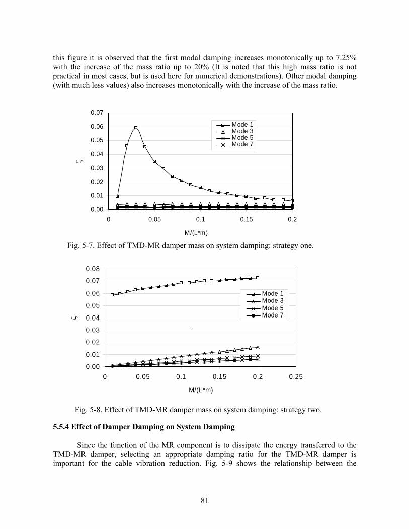
this figure it is observed that the first modal damping increases monotonically up to 7.25% with the increase of the mass ratio up to 20% (It is noted that this high mass ratio is not practical in most cases, but is used here for numerical demonstrations). Other modal damping (with much less values) also increases monotonically with the increase of the mass ratio.

Fig. 5-7. Effect of TMD-MR damper mass on system damping: strategy one.

0.00

0.01

0.02

0.03

0.04

0.05

0.06

0.07

0 0.05 0.1 0.15 0.2

M/(L*m)

ζ

Mode 1Mode 3Mode 5Mode 7

Fig. 5-8. Effect of TMD-MR damper mass on system damping: strategy two.

0.00

0.01

0.02

0.03

0.04

0.05

0.06

0.07

0.08

0 0.05 0.1 0.15 0.2 0.25

M/(L*m)

ζ

Mode 1Mode 3Mode 5Mode 7

`

5.5.4 Effect of Damper Damping on System Damping Since the function of the MR component is to dissipate the energy transferred to the

TMD-MR damper, selecting an appropriate damping ratio for the TMD-MR damper is important for the cable vibration reduction. Fig. 5-9 shows the relationship between the

81

system modal damping and the damper damping ratioξ . It can be seen that in this figure that the first modal damping increases from zero when the damping ratio ξ increases from zero, reaches the maximal value of 7.58% at 3.0=ξ , and reduces toward zero thereafter. For higher modes, the trend is similar except that the modal damping reaches smaller maximum values (the maximum third modal damping is about 2%) at larger values of ξ . 5.5.5 Vibration Reduction of Higher Modes

From the previous discussions, we can conclude that the mid-span placement and the first mode tuning of the damper are very effective to improve the system damping if appropriate cable-damper parameters are chosen. However, since the mid-span point is actually a node of the second mode, any damper placed there will have no reduction effect on the second mode vibration. Therefore, a TMD-MR damper tuned to the second modal

frequency mT

Lf π2

2 = of the pure cable is placed at the 1/4th point to investigate the

vibration reduction effectiveness for higher modes.

Since the second strategy can achieve a better first modal damping, only the second strategy is considered here. Fig. 5-10 shows the relationship between the system modal damping and the stiffness change ( is the same as before.). Though called the second mode tuning, the damper is also tuned to other modes by changing the stiffness

0KK . The damper

location is the only difference between this case and that for the first mode tuning with the second strategy (Fig. 5-6). The curves are similar for these two cases, but with different maximum modal damping and corresponding stiffness values. The maximum first modal damping is almost the same as that of the first mode tuning. However, the second and third modal damping are much larger, especially for the second modal damping, which is increased from zero to about 5.52%. Since the damper is located at the node for the forth mode and has no reduction effect so that the corresponding modal damping is not shown in the figure.

Fig. 5-9. Effect of TMD-MR damper damping ratio on system damping.

0.000.010.020.030.040.050.060.070.080.090.10

0 0.5 1 1.5 2 2.5

ξ

ζ

Mode 1Mode 3Mode 5Mode 7

82

Fig. 5-10. Effect of TMD-MR damper stiffness on system damping, second mode tuning.

0.000.010.020.030.040.050.060.070.080.090.10

0.01 0.1 1 10 100

ζ

Mode 1Mode 2Mode 3Mode 5

K/K0

The maximum modal damping and corresponding optimal stiffness for both mode tunings are listed in Table 5-3. From this table, the optimal stiffness for the maximum first modal damping seems to be “pushed back” less than 1.0 when the damper is placed at the 1/4th point that targets the second mode. The observations indicate that the damper installed at the 1/4th point can be efficient for both the first and second modes, perhaps as well as for other higher modes such as mode 3 and 5, as long as the stiffness is adjusted to the optimal values. Therefore, for a damper with a wide adjustable stiffness range, maybe the 1/4th is a better position to place the damper than the mid-span overall since it can be tuned to either the first or the second mode as needed. Table 5-3. Comparison of maximum modal damping and corresponding optimal stiffness for

different mode tuning

First mode tuning Second mode tuning Modal damping 1ζ 8.88% 8.95%

First mode Optimal stiffness ( ) 0/ KK 2.04 0.44

Modal damping 2ζ 0 5.52% Second mode Optimal stiffness

( ) 0/ KK N/A 4

Modal damping 3ζ 5.84% 6.56% Third mode Optimal stiffness

( ) 0/ KK 11.1 11.1

83

Fig. 5-11 shows the relationship between the system modal damping and the mass change for the second mode tuning for a given frequency ratio 2/1=ρ and a damping ratio 1.0=ξ . It is shown in this figure that the second modal damping decreases monotonically when the mass ratio increases. Other modal damping increases when the mass ratio increases, especially for the third mode. This observation indicates that with the change of the mass ratio, the optimal frequency ratio of the second mode changes and is pushed away from the frequency tuned for the pure cable ( 2/1=ρ ), while the optimal frequency ratio of the third mode becomes closer. This observation also implies that the damper may need to be tuned to the frequency of the combined cable-damper system, not the pure cable.

Table 5-4 shows the modal damping for 5% and 20% mass ratios for both the first and

second mode tunings. From this table, we can observe that when the damper changes from a first mode tuning to a second mode tuning, the first modal damping for the cases of both 5% and 20% mass ratios decrease significantly while the second and third modal damping increase correspondingly, especially the second modal damping. However, the level of the change depends on the mass ratio. This indicates that if the TMD-MR damper is tuned to a specific cable mode, that cable modal damping will be enhanced in general. However, the change of the modal damping for other modes depends on other parameters. This actually reflects the dependence of the modal damping on the relationship between the cable and the TMD-MR damper overall, not just the frequency.

Table 5-4. Comparison of modal damping for different mode tuning

Mass ratio Modal damping for first mode tuning

Modal damping for second mode tuning

5% 6.39% 0.08% First mode 20% 7.23% 0.26% 5% 0 5.50% Second mode 20% 0 3.56% 5% 0.40% 1.05% Third mode 20% 1.58% 3.53%

Fig. 5-12 shows the relationship between the system modal damping and the damping

ratio change with the second mode tuning. From this figure, similar observations to Fig. 5-9 (the first mode tuning) are obtained. The maximum modal damping of each mode is compared in Table 5-5 for these two mode tunings. From this table, we can observe that when the first mode tuning is changed to the second mode tuning, the maximum first modal damping decreases dramatically; the maximum second modal damping increases significantly; and the maximum third modal damping decreases marginally. In addition, when the TMD-MR damper is tuned to the second mode cable vibration, the third mode can achieve a comparative modal damping ratio with a smaller damper damping ratioξ .

84

Fig. 5-11. Effect of TMD-MR damper mass on system damping, second mode tuning.

0.00

0.01

0.02

0.03

0.04

0.05

0.06

0 0.05 0.1 0.15 0.2 0.25

M/(L*m)

ζ

Mode 1Mode 2Mode 3mode 5

0.00

0.01

0.02

0.03

0.04

0.05

0.06

0.07

0.08

0 0.5 1 1.5 2

ξ

ζ

Mode 1Mode 2Mode 3Mode 5

Fig. 5-12. Effect of TMD-MR damper damping ratio on system damping, second mode tuning.

85

Table 5-5. Comparison of modal damping with damping ratio change of MR component for different mode tuning

First mode tuning Second mode tuning

Modal damping 1ζ 7.58% 0.45% First mode Optimal damper damping

ξ 0.3 0.7

Modal damping 2ζ 0 6.86% Second mode Optimal damper damping

ξ N/A 0.3

Modal damping 3ζ 2.75% 2.32% Third mode Optimal damper damping

ξ 1 0.3

5.6 Example for a TMD-MR Damper Design

Detrimental incidences of wind-rain induced cable vibrations have been widely reported for cable-stayed bridges recently (Hikami 1986, Matsumoto et al. 1992). In the following discussions, the emphasis is placed on the wind-rain vibration issues.

Irwin (1997) proposed the following criterion to control the wind-rain induced cable

vibration,

αζ≥= 2pD

mSc (5-28)

where is the Scruton number; p is the mass density of air; is the outside diameter of cable; and

cS Dα is the limiting value for Scruton number. The above relationship can be

rewritten as

μααζ =≥

mpD2

(5-29)

where the mass parameter μ is defined as )( 2pDm=μ . Therefore, to meet the above stated criterion, the damping ratio of the cable needs to meet the requirement of Eq. (5-29). Based on available test results, Irwin (1997) proposed a minimum α of 10. The modal damping of a stay-cable is composed by the intrinsic damping and the additional damping provided by damping devices. The former is typically low and cannot be reliably estimated. A range of damping ratios of 0.05%–0.5% has been reported for stay cables (‘‘Recommendations’’ 1998). In this discussion, the intrinsic damping of the cable is conservatively ignored. The following example is used for demonstrating a preliminary design process.

This example has been used by Tabatabai and Mehrabi (2000). Assume that a cable with the properties listed in Table 5-6 is in need of a TMD-MR damper to suppress wind-rain

86

induced vibrations. To design a TMD-MR damper with its frequency tuned to the first mode, the following process can be followed. 1) Determine the demanded modal damping ratio Since the mass parameter μ can be calculated as 1747)( 2 == pDmμ , the demanded modal damping is determined from Eq. (5-29) as, %57.00057.01747101 ===≥ μαζ (5-30) 2) Determine the TMD-MR parameters

Since the TMD-MR damper is tuned to the first mode, it should be placed at the mid-span to achieve the best reduction efficiency. Following the common practice, the mass ratio of the damper is chosen as 2%, from which the mass of the damper is determined as kgmLM 2.21209.114*93*02.0**%2 === (5-31)

Table 5-6. Properties of example cable

m (kg·m-1) L (m) T (N) P (kg/m3) D (m) 1cω (sec-1) 114.09 93 5.017*106 1.29 0.225 7.08

The frequency ratio is then chosen approximately as 0.1=ρ since it is a fundamental

mode tuning, from which the stiffness of the TMD-MR damper can be determined as

mNmT

LMK /3.6403)

09.11410*017.3

9314159.3(*2.212)( 2

62 ===

π (5-32)

The developed design aid curve in Fig. 5-13 is then referred to determine the

equivalent damping ratio for the MR component. If an actual modal damping %11 =ζ is chosen so that a safety factor of 75.1%57.0/%1 = can be achieved, the equivalent damping ratio ξ is thus obtained as 2.6% by interpolation. Once the required equivalent damping ratio of the MR component is known, a preliminary design for the MR component (such as the MR liquid and current) can be performed (Li et al. 2000), which is out of the scope of this study. 0.00

0.01

0.02

0.03

0.04

0.05

0.06

0.07

0 0.05 0.1 0.15 0.2 0.25 0.3

ξ

ζ Mode 1Mode 2Mode 3Mode 5

Fig. 5-13. Design curve of 2% mass ratio, first mode tuning.

87

For the same cable, if the damper is located at the 1/4th point of the cable length to target the second mode vibration control, the stiffness of the damper is determined as,

mNmT

LMK /2.25613)

09.11410*017.3

9314159.3(*2.212*4)(4 2

62 ===

π (5-33)

Then, similarly, Fig. 5-14 is referred to determine the equivalent damping for the MR component. An actual modal damping %11 =ζ is also chosen so that the equivalent damping ratio ξ is obtained as 2.54%.

Fig. 5-14. Design curve of 2% mass ratio, second mode tuning.

0.00

0.01

0.02

0.03

0.04

0.05

0.06

0.07

0 0.05 0.1 0.15 0.2 0.25 0.3

ξ

ζ Mode 1Mode 3Mode 5Mode 7

In addition to the wind-rain induced cable vibrations, other types of cable vibrations such as due to vortex excitation, galloping, etc. are also concerned. However, if a target cable damping ratio is defined for these specific types of vibrations, the design process proposed here is also applicable. For a refined optimal design, much more calculations are necessary to construct design curves that relate the damping ratio of the TMD-MR to the system modal damping of the cable-damper system under different parameters. Simultaneous multimode cable vibration control by using multiple TMDs and adaptive control also deserve further studies, which will be pursued by the writers once the basic behavior of the cable-TMD-MR system is fully understood. 5.7 Conclusions

Free vibrations of a taut cable with a hung-on TMD-MR damper that has been proposed by the writers in the companion study have been investigated in the present study, which is of considerable practical interest since the cable vibration problem becomes a serious issue for cable-stayed bridges. An analytical formulation of the complex eigenvalue problem has been used to derive an equation for the eigenvalues, which represents the dynamic property of the cable-TMD-MR system. The solution of the complex equation reveals the attainable system modal damping ratios iζ and corresponding oscillation frequencies. The

88

solution of the complex equation provides a better understanding of the dynamic characteristics of the cable-TMD-MR system with corresponding system parameters, such as nonoscillatory decaying and nondecaying oscillation vibrations.

The position, stiffness, mass, and damping ratio of the damper affect the cable-TMD-

MR system dramatically. If the damper is tuned to the fundamental natural frequency of the cable, the first modal damping will increase when the damper moves from the end and reaches the maximum value of 6.27% at the mid-span of the cable. The damper provides a maximum second modal damping when it is installed at the 1/4th point of the cable and has no damping effect for the second mode when it is installed at the mid-span. Since the first modal damping is of primary practice interest, the damper is placed at the mid-span of the cable for other parametric study with the first mode tuning. Parametric results show that the maximum first modal damping achievable is larger than that of a viscous damper. The parametric study also shows the importance to balance the two relative pairs of parameters. One is between the cable and the damper, and the other is between the TMD and the MR components. The former is mainly discussed in the companion study (Cai et al. 2006). In the case of a very strong TMD with a weak MR component, though the vibration can be transferred effectively from the cable to the damper, the vibration transferred cannot be dissipated effectively. On the contrary, a very strong MR component with a weak TMD will work as a rigid bar so that it cannot help transfer effectively the vibration from cable to the damper. As a result, both of these two cases result in a very small first modal damping.

Profound understanding of the dynamics of the cable-damper system makes the TMD-MR damper design for cable vibration control possible. The example with both the first mode and the second mode tuning shows that the system modal damping requirements to suppress a taut cable vibration can be achieved in a straightforward format by choosing a required equivalent TMD-MR damping ratio. Other types of dampers can also be used as long as they provide the required equivalent damping ratio. A simple model for the cable and the MR component used in this study represents the essence of the dynamic properties of the cable-damper system. However, a refined model for the cable-TMD-MR damper may be considered in the oncoming research such as considering the effect of the cable and the stiffness adjustability of the MR component. The developed procedure provides an analytical and/or numerical tool to understand the behavior of the cable-TMD-MR system, which is necessary for a rational design of the TMD-MR damper and for developing a robust control strategy for the cable vibration.

Δ−p

5. 8 References Cai, C. S. and Wu, W. J. (2004). “Development of an Adaptive Damper for Cable Vibration

Control.” A Final Report, Project No. NCHRP-92, submitted to the IDEA Program, Transportation Research Board, National Research Council, Louisiana State University, Baton Rouge, Louisiana.

89

Cai, C. S., Wu, W. J., and Araujo, M. (2006). “Cable Vibration control with a TMD-MR Damper System: Experimental Exploration.” Journal of Engineering Structures (submitted).

Carne, T. G. (1981). “Guy Cable Design and Damping for Vertical Axis wind Turbines.”

Report No. SAND80-2669, Sandia National Laboratories, Albuquerque, N.M. Hikami, Y. (1986). “Rain vibrations of cables in cable-stayed bridges.” Journal of Wind

Engineering, 27, 17-28 (in Japanese). Irvine, H. M. and Caughey, T. K. (1974). “The linear theory of free vibrations of a suspended

cable..” Proceedings of Royal Society (London), A341, 299-315. Irvine, H. M. and Griffin, J. H. (1976). “On the Dynamic Response of A Suspended Cable.”

Earthquake Engineering and Structural Dynamics, 4(4), 389-402. Irvine, H. M (1978). “Free Vibration of Inclined Cables.” Journal of Structural Division,

proceedings of the ASCE, 104(ST2), 343-347. Irvine, H. M. (1981). “Cable Structure.” MIT Press Series in Structural Mechanics,

Cambridge, Massachusetts, and London, England, 1981. Irwin, P.A. (1997). “Wind Vibrations of Cables on Cable-Stayed Bridges.” Proceedings of

ASCE Structures Congress. Vol. 1, April 1997, 383-387. Johnson, E. A., Christenson, R. E., and Spencer, B. F. (2003). “Semiactive damping of cables

with sag.” Computer-Aided Civil and Infrastructure Engineering, 18, 132-146. Krenk, S. (2000). “Vibrations of a taut cable with an external damper.” Journal of Applied

Mechanics. Vol. 67, 772-776. Krenk, S. and Nielsen, S. R. (2002). “Vibrations of a shallow cable with a viscous damper.”

Proceedings of Royal Society (London), A458, 339-357. Li, W. H., Yao, G. Z., Chen, G., Yeo, S. H. and Yap, F. F. (2000). “Testing and Steady State

Modeling of a Linear MR Damper under Sinusoidal Loading.” Smart Materials and Structures, Vol. 9, 95-102.

Main, J. A., and, Jones, N. P. (2002). “Free vibration of taut cable with attached damper. I:

linear viscous damper.” Journal of Engineering Mechanics, 128(10), 1062-1071. Matsumoto, M., Shirashi, N., Shirato, H. (1992). “Rain-wind induced vibration of cables of

cable-stayed bridges.” J. Wind Engineering and Industrial Aerodynamics, 44, 1992: 2011-2022.

90

Pacheco, B.M., Fujino, Y., and Sulekh, A. (1993). “Estimation curve for modal damping in stay cables with viscous damper.” Journal of Structural Engineering., 119(6), 1961-1979.

‘‘Recommendations for stay cable design, testing and installation.’’ (1998). 4th Draft, Post-

Tensioning Institute Committee on Cable-Stayed Bridges. Starossek, U. (1994). “Cable dynamics - A review.” IABSE, Structural Engineering

International, 4(3), 171-176. Tabatabai, H., and Mehrabi, A. B. (1999). “Tuned dampers and cable fillers for suppression of

bridge stay cable vibrations.” Final report to TRB IDEA program, Construction Technology Laboratories, Inc, Skokie, Illinois.

Tabatabai, H., and Mehrabi, A. B. (2000). “Design of mechanical viscous dampers for stay

cables.” Journal of Bridge Engineering., 5(2), 114-123. Yamaguchi, H., and Fujino, Y. (1998). “Stayed cable dynamics and its vibration control.”

Bridge aerodynamics, A. Larsen and S. Esdahl, eds., Balkema, Rotterdam, The Netherlands, 235–253.

91

CHAPTER 6. CABLE VIBRATION REDUCTION WITH A HUNG-ON TMD SYSTEM – PART I: THEORECTICAL STUDY*

6.1 Introduction

As key load-carrying members of cable-stayed bridges, stay cables are of primary

importance to secure the safety of the entire structure. Since cables are generally flexible, relatively light, and low energy-dissipative because of their inadequate intrinsic damping, they are susceptible to external disturbances such as vortex shedding, rain-wind induced vibration, vehicle-induced vibration, and other excitations due to parametric disturbance caused by the motion of either the bridge deck or towers.

To suppress the problematic vibrations, a common practice is to install mechanical

(including viscous/oil and Magnetorheological (MR)) dampers with one end connected to the deck and the other end connected to the cable at a distance typically 2-4% of the cable span length from the lower end. A lot of research effort has been exerted on the viscous/oil dampers (Pacheco et al. 1993, Yu and Xu 1998, Xu and Yu 1998, Johnson et al. 2003). MR dampers have recently been used due to their advantages over traditional mechanical dampers, such as their adjustable damping force, mechanical simplicity, reliability, and minimum power requirement (Chen et al. 2003). Nevertheless, the attached mechanical dampers may not be most effective because their positions are restricted at the cable ends. Tuned Mass Dampers (TMD) were therefore proposed, which can be placed anywhere along the cables to overcome the shortcomings of the mechanical dampers (Tabatabai and Mehrabi 1999). However, the TMDs’ effectiveness is sensitive to the cable vibration frequency, which makes TMDs difficult to be implemented in a complicated system where the cable vibration frequency is difficult to be predicted due to various uncertainties. A newly proposed TMD-MR (Tuned Mass Damper-Magnetorheological) damper system has been demonstrated both experimentally and theoretically as a promising means for cable vibration reduction since it combines both the advantages of the position flexibility of the TMDs and the adjustability of the MR damper (Cai et al. 2005, Wu and Cai 2005). Wu and Cai (2005) conducted an analysis on the free vibration problem of a taut horizontal cable with a TMD-MR damper placed along the cable and made a tentative discussion on the modal damping of the cable-damper system.

Though the theoretical analysis based on the taut horizontal cable model may reveal

the essential characteristics of the cable-damper system, the investigation based on an inclined cable with a small sag is definitely more accurate and gives more information that a taut horizontal cable cannot provide. Therefore, a theoretical model based on an inclined cable with a small sag is considered in this study. In this more refined model, both the cable parameters such as cable geometry-elasticity parameter, cable internal damping, cable inclination, and the damper parameters such as the damper position, mass, stiffness, and damping ratio are taken into consideration. The formulation for a planar vibration problem of a cable-TMD-MR system is thus presented in this study. Special cases are discussed and some

* Reprinted by permission of the Journal of Vibration and Control, Sage Publication Ltd. Copyright(©SAGE Publications, 2006)

92

simpler models can be retrieved. Complex solutions of the derived equations and their physical meaning are discussed. The parametric study based on this formulation is discussed in the companion study (Wu and Cai 2006). 6.2 Refined Theory for Inclined Cable with a Hung-on TMD Damper 6.2.1 Governing Equation for a Cable-TMD System

The present study concerns the planar vibration of an inclined cable with a small sag

installed with a hung-on TMD-MR damper. The prototype cable-TMD-MR system under consideration (Cai et al. 2005) is sketched in Fig. 6-1(a), where the circular damper is clipped on the cable and vibrates in a way perpendicular to the cable chord. The TMD-MR damper is modeled in Fig. 6-1(b) as an equivalent system consisting of a variable spring K , a dashpot with an adjustable damping coefficient C , and a mass M . The damping coefficient represents the equivalent damping of the MR damper and can be obtained by a linearization process (Li et al. 2000). Since the parametric study has been carried out in the companion study (Wu and Cai 2006), the variability of

C

K and is not considered in the governing equations in the present study. Therefore, the TMD-MR system is simply called TMD or damper hereafter, and the results obtained are also applicable for other types such as TMDs with viscous dampers.

C

In this calculation model (shown in Fig. 6-1(b)), the damper is hung on the cable at an

intermediate point, dividing the cable into two segments, with a cable chord length of and , respectively. The notation without subscript is used to represent either segment. Without

losing generality, it is assumed that . The x coordinate is taken as along the cable chord direction and the y coordinate is perpendicular to the x coordinate and along the downward direction. The left support of the cable is taken as the origin of the Cartesian coordinate system for the first segment and the right support as the origin for the second segment. Therefore, the planar equation of motion for each cable segment can be expressed by the following two partial differential equations

1l

2l

12 ll >

θτ sin)])([( 2

2

mgtuc

tum

su

sddxT

sf x +

∂∂

+∂∂

=′∂

∂+

′+

′∂∂

+ , (6-1)

θτ cos)])([( 2

2

mgtvc

tvm

sv

sddyT

sf y −

∂∂

+∂∂

=′∂

∂+

′+

′∂∂

+ . (6-2)

where and are the distributed cable force along the x and y directions, respectively; xf yf T is the static cable tension; τ is the dynamic cable tension; s′ is the Lagrangian coordinate in the unstrained cable profile; u and v are the cable dynamic displacement components along the x and y coordinates measured from the static equilibrium position of the cable, respectively; and are the distributed cable mass and damping coefficient per unit length, respectively; is the time;

m ct g is the gravitational acceleration; and θ is the inclined cable

93

angle measured from the horizontal axis. The notation )()(od

d • denotes the derivative of “ • ” with

respect to “ ”, and o)()(o∂•∂ means the partial derivative of “ • ” with respect to “ o ”.

MR damper

Cut to clip on cable

MR fluids that can change to

semi-solid

Mass of TMD

Cable

Inner shell

Accelerometer

(a)

Fig. 6-1. Calculation model: (a) prototype TMD-MR damper system; (b) the inclined sag cable with a TMD damper

(b)

l1

l2

K C

My

x

x1

x2

94

To simplify the calculation without losing much accuracy, the following assumptions are made:

(1) The tension force in the cable is large compared to its weight so that the sag and the slope of the cable are small, and also large compared to the total external force to keep the system in the linear range.

(2) The bending stiffness and intrinsic damping of the cable is small and therefore can be neglected at large.

(3) The displacement component along the x direction is not important and may be ignored, based on the first assumption.

When the cable without damper is in its static equilibrium position, the dynamic tension and corresponding displacement components vanish from Eqs. (6-1) and (6-2), the horizontal component of the cable tension force can be obtained as a constant along the cable, and the static cable profile can thus be expressed as,

)1(2

)cos(lxxy −=

θε (6-3)

where is the length of cable chord and l ε is the ratio of the cable weight to the tension force, as

1)cos( <<= θεH

mgl (6-4)

where H is the constant horizontal component of the cable tension force, and the inequality is obtained directly from the first assumption. Terms of higher order on ε (such as ) are dropped, and if the inclination angle

2εθ turns to be zero, the parabolic static profile for a

horizontal cable can be obtained. Therefore, the sag of the mid-span of an inclined cable can be obtained as

8

)cos(θεld = . (6-5)

As Irvine (1981) pointed out, the linear cable assumption is applicable for a horizontal

profile with . This requirement is easily satisfied since8/ld ≤ ε is assumed to be much less than 1.

After the static equilibrium equations under cable self weight are subtracted from the

dynamic equations of motion (Eqs. (6-1) and (6-2)), the assumptions are applied, and the terms of higher order of ε are neglected, the equation of motion can be simplified as

tvc

tvm

xdydh

xvHf y ∂

∂+

∂∂

=+∂∂

+ 2

2

2

2

2

2

cosθ (6-6)

where is defined as h

sddxh

′= τ . (6-7)

95

The term tvc

∂∂ , representing the cable distributed viscous damping, is usually

neglected since it is very small and hard to measure in real application. However, this term is kept here for forced vibrations in case that the cable response without a TMD would become infinite

fter an elastic deformation, the element with a length of

.

sd ′A at the static equilibrium will be retched to a length of sd ′ st . The elasticity relation of the cable can be written as

sv

sddy

su

sddx

dydx

dydxvdyudxsd

sdsdEA ′∂

∂′

+′∂

∂′

≈+

+−∂++∂+=

′′−′

=22

2222 )()(τ (6-8)

where E is the Young’s modulus of the cable and is the area of the cable cross section. Multip Eq. (6-8) by and considering Eq. (6-7), then integrating over the equation and using the fixed boundary condition for both cable ends leads to

Alying 2)/( dxsd ′

∫∫ =∂∂

=ll

e vdxlddx

xv

dxdyL

EAh

02

0

8 (6-9)

where is the effective cable length, defined as

eL

llddx

dxsdL

l

e ∫ +≈′

=0

23 ])(81[)( . (6-10)

hile the damper will affect the system performance, the above equations for each

cable segment are independent of the existent damper. First proposed by Irvine and Caughey (1974) for a horizontal cable, these equations revealed the relation between the additional tension force and the average dynamic displacement along the cable.

he installation of the TMD damper separates the cable into two segments and causes the discontinuity of the cable slope at the place where the damper is located. However, one more force boundary condition at the hung-on point of the damper is provided as

W

T

)()()(cos

1111

2211

11

2

2

1

1

dtdv

dtdvCvvK

xv

xvH d

lxdlx

lxlx

−+−=∂∂

−∂∂

−=

=

==θ

(6-11)

where and are the displacements of the cable for the corresponding segments, with displacement boundary conditions as

1v 2v0)0()0( 21 == vv and cvlvlv == )()( 2211 c

cable displacement at the TMD damper location. v is the damper displacement that is along the per

. is the v

d

pendicular direction to the cable chord.

Meanwhile, the equilibrium of the damper itself shows

0)()(2

11 =−−+−

vdMdvdvCvvK ddd . (6-12) 211= dtdtdtlx

MD system is ready to be solved.

11=lx

With these equations, the cable-T

96

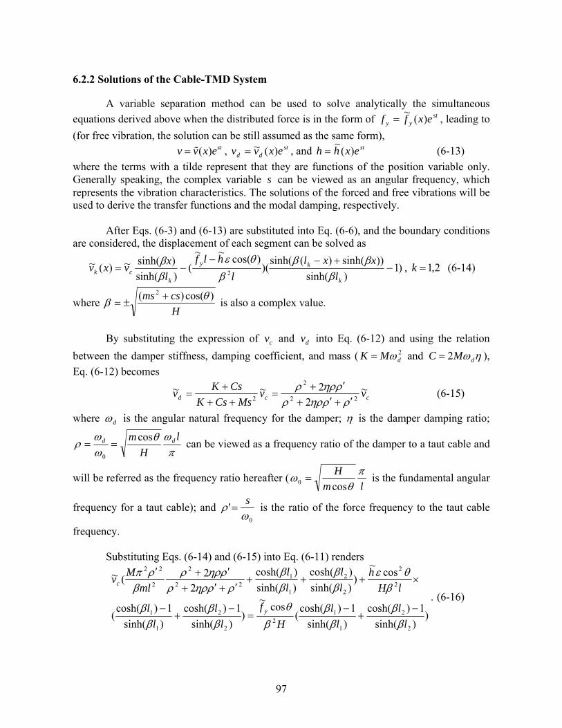
6.2.2 Solutions of the Cable-TMD System A variable separation method can be used to solve analytically the simultaneous

equations derived above when the distributed force is in the form of styy exff )(~

= , leading to (for free vibration, the solution can be still assumed as the same form),

stexhh )(~= (6-13) ( ) stv v x e= % , st

dd exvv )(~= , and where the terms with a tilde represent that they are functions of the position variable only. Generally speaking, the complex variable s can be viewed as an angular frequency, which represents the vibration characteristics. The solutions of the forced and free vibrations will be sed to derive the transfer functions and the modal dam

u ping, respectively.

After Eqs. (6-3) and (6-13) are substituted into Eq. (6-6), and the boundary conditions are considered, the displacement of each segment can be solved as

)1)sinh(

))sinh()(sinh()(

)cos(~~()sinh(~)(~ +−−

−= yck

xxlhlfxvxvββεβ

)sinh( 2 −k

k

k lll ββθ

β (6-14) , 2,1=k

Hcsms )cos()( 2 θ+where β ±= is also a complex value.

per

By substituting the expression of cv and dv into Eq. (6-12) and using the relation

between the dam stiffness, damping coefficient, and mass ( 2dMω= and K ηωdMC 2= ),

Eq. (6-12) becomes

ccd vvMsCsK

v ~2

2~~222 ρρηρρ ′+′+

=++

= (6-15)

where d

CsK 2 ρηρρ ′++

ω is the angular natural frequency for the damper; η is the damper damping ratio;

πωθ

ωω

ρl

Hm dd

0

=cos

= can be viewed as a frequency ratio

ill be referred as the frequency ratio hereafter (

of the damper to a taut cable and

lm θω

cos0 = is the fundamental angular H πw

frequency for a taut cable); and 0

'ω

ρ = is the ratio of the force frequency to the taut cable

frequency. Substituting Eqs. (6-14) and (6-15) into Eq. (6-11) renders

s

)sinh()sinh(

())sinh(

))sinh(

(

cos

1)cosh(1)cosh(cos~

1cosh(1)cosh(

~)

)sinh()sinh(2( 2

21222

llfl

lHllmlvc

ββθβ

βββρρηρρβ

−−−−

×+++′+′+

. (6-16)

)

)cosh()cosh(2~

2

1

12

2

2

1

1

221

222

llHll

l

hllM

y

βββββ

β

θεββρηρρρπ

+=+

′+′

2

97

S

ubstituting Eq. (6-14) into Eq. (6-9), we can obtain

)sinh(2)cosh(2

)sinh(2)cosh(2

(cos~

)

)sinh(2)cosh(2

)sinh(2)cosh(2

(cos~)

)sinh(cosh(

)sinh(1)cosh(

(~2

2

1

12

2

2

2

1

1

ll

ll

lHll

ll

vc ββ

ββ

βθε

ββ

ββ

−−

+−

++−

)

1)

2

2122

33

ll

ll

Hfll

h

y

ββ

ββ

β

θ

λββ −

−+

−=−

−

(6-17)

ial stiffness to the cable geometry stiffness nd thus called the cable geometry-elasticity parameter here

lβ1

where is proportional to the ratio of the cable ax2λa after. It can be written as

θθεθλ

cos/)(coscos)8( 2222

HAE

LL

HLlAE

ld

ee

== . (6-18)

as zero), the following equation should be satisfied

The simultaneous equations (6-16) and (6-17) are applicable for both free vibration

( 0=yf ) and forced vibration as mentioned before. For a free vibration problem, if a non-trivial solution is desired (The distributed cable damping c is chosen

0=)

)sinh(2)cosh(2

)sinh(2)cosh(2

())sinh()cosh(

)sinh()cosh(

2

33

2

2

1

1

2

2

1

1 −−−

+−

×++λ

ββββ

ββ

ββ

ββ ll

ll

ll

ll

ll

(6-19)

W

22()

)sinh(1)cosh(

)sinh(1)cosh(

( 22

2

2

222

2

2

1

1

′+′+′+′

−−

+−

ρρηρρρηρρ

βρπ

ββ

ββ

mlM

ll

ll

ith the notations llr /11 = , llr /22 = , lββ 5.0=′ , and the following hyperbolic identical equations

)5.0cosh()5.0cosh(

)5.0sinh()sinh(

1)cosh()sinh(

1)cosh(

2

2

1

1 ll

ll

l

21 ll βββ

ββ

ββ

=−

+− (6-20-a)

)5.0sinh()5.0sinh(

)coth()coth(1

21 lll

β)sinh(

2ll

ββββ =+ , (6-20-b)

q. (6-19) can thus be simplified as E

)}4)(cosh()){sinh(h(4 sin)})(cosh()cosh( 3221

)){sinh(sinh()sinh()/'(4)/'(4

)/'(44

32

212

2

β

2

λβββββ

λβββ −=′+′′′− rr

βββπβπβηρ

πβηρρβ

′

′′′++

+′ rrmr (6-21)

where

ρ

+′′−′′

mlMmr = is the mass ratio between the TMD and the cable.

This dimensionless eigenvalue equation in terms of β ′ (or

portance for the concerned cas ) is of fundamental

rongly non-linear with respect to its parametersim ble-TMD free vibration problem. Obviously, Eq. (6-21) is st . Therefore, a thorough investigation of each dimensionless parameter, including the mass ratio rm , the frequency ratio ρ , the damper damping ratio η , the damper position 1r (or 2r ), and the cable geometry-elasticity parameter

2λ , is important in understanding the performance of the cable-TMD system, which will be carried out in the companion study (Wu and Cai 2006). Although the cable inclined angle θ

98

is not explicitly expressed, it is still very important since it affects the parameters ρ and .

For the forced vibration problem with a harmonic force of

2λOnce the eigenvalue is obtained, the mode shape can be solved easily with Eq. (6-14).

( ) sj t

y yf f x e ω= ,

simultaneous Eqs. (6-16) and (6-17) can be solved for

%

and h~cv~ . Therefore, the displacement cable point at any time th Eqs. (6-13) and (6-14).

6.3 Discussions of Special Cases for Free Vibrations

io lverify th ivations. F

is no TMD damper attached to the cable, the left hand side of Eq. (6-21) equation reduces to

for each can be directly obtained wi

Some special cases for free vibrat n prob ems can be retrieved from the derived

fundamental equations, which serves as an indirect way to e der or example, when theredoes not exist and the

0)}4)(cosh()){sinh(sinh( 32 =′+′′−′′ β

λββββ . (6-22)

This equation includes a solution for antisymmetric modes with 0)sinh( =′β and a solution

th for symmetric modes wi )4)(cosh()sinh( 32 β

λβββ ′+′′−′ =0, from which the results can be

contain the solution for the cable static profile, which corresponds to 0obtained for the horizontal cable when the inclined angle is set to be zero. Both equations

=′β .

When the cable geometry-elasticity parameter approaches infinity, i.e., →∝2λ ,

obtained for

meaning that the axial/elastic stiffness of the cable is infinitely large, a special case is an inextensible cable with a damper installed. When the cable geom

parame r approaches zero, i.e., , meaning that the tension force is infinitely large so that the

etry-elasticity 02 →λte

re is no cable sag, Eq. (6-21) reduces to

)cosh()cosh()sinh()sinh()cosh()sinh(

)/'(4)/'(4)/'(44

212122

2

rrrrmr ββββ

ββπβπβηρρ

πβηρρβ′′′′

′′−=

+++′ . (6-23)

special case is obtained from Eq. (6-23) for a taut cable with an installed damp

A er as

))coth()(coth(2)/'(4)/'(4

)/'(44 2122

2

rrmr ββπβπβηρρ

πβηρρβ ′+′=++

+′ , (6-24)

since th s: e following hyperbolic identical equation always hold

))coth()(coth(2)cosh()cosh()sinh()sinh(

)cosh()sinh(21

2121

rrrrrr

ββββββ

ββ ′+′≡′′′′

′′− . (6-25)

If the inclination is zero, Eq. (6-24) is exactly the same as the governing equation for a taut horizontal cable with a TMD damper, which was discussed in Wu and Cai (2005). 6.4 Discussions of Solutions for Free Vibrations

Usually, the complex value s (similarly for β and 'β ) can be expressed as the sum of

s real and imaginary parts as it

iii js ϕσ += (6-26)

99

where )( iii ζωσ −= and )1( iii ζωϕ −= (It can be proven that if '2 β is a solution of Eq. (6-21), then its conjugate is also a solution. Therefore, we can discuss only the solution with a positive imaginary part. Similarly, for simplicity of the narrative, we assume that the damping

iζ is not larger than 1. Actually, the performance of the system with a damping 1>iζ is

). 1−=jsimilar to that with a damping 1=iζ is the imaginar m Eq. (6-26), the

amped system frequency can be obtained as

y root. Fro22

iii ϕσω += d and the system m ng

can be obtained as

odal dampi

)2/1(2

2

)1( −+=i

ii σ

ϕζ for the i-th mode, respectively. Therefore, the complex

solution

The response characteristics of the cable-damper system to the frinvestigation on the location of the complex solution

lution is impossible to be located at the right half of the co

s contains information of both the damped frequency and the modal damping for the cable-damper system.

ee vibrations can be

investigated through an s . First of all, the so mplex plan ( 0>iσ ). Otherwise, the corresponding modal damping iii ωσζ /−= will be negative and the

e vibration will become infinite when the tim . Therefore, the real part of the solution should not be larger than zero. Whenthe imaginary axis (

magnitude of the response to a fre e lasts the solution is on

0=iσ ), the modal damping iζ is also equal to zero so th n is sinusoidal with a constant amplitude as the time goes by. When the solution is on the left real axis (

at the vibratio

0<iσ and 0=iϕ ), the damping ratio is equal to 1.0, the maximum system

)2/1(2

2

)1(=ϕ

ζdamping ratio achievable as restricted by the definition −+i

ii σ

. Under this

conditi Oon, the free vibration will decrease without oscillation. nly when the solution is on the left hand side of the imaginary axis but not on the real axis ( 0<iσ and 0>iϕ based on the definition) will the cable-damper system vibrate periodically with a decaying vibration magnitude.

The cable vibration mitigation with TMD dampers can be considered as a process to

change the solution location of the governing equation of the pure cable (Eq. (6-22)) by adding the corresponding terms related to a TMD (the left hand side of Eq. (6-21)). There are infinite solutions for the governing equation of the pure cable (Eq. (6-22)), laid in sequence on the imaginary axis with zero corresponding modal damping, as shown in Fig. 6-2 for the first five modes marked by light blocks, The solution for the TMD itself, indicated by the light diamon

2 s

le vibration reduction totally depends

d, shifts the pure cable solutions to new positions represented by the dark blocks. At the mean time, the installation of the TMD damper actually brings one more solution to Eq. (6-21), compared to the number of solutions of Eq. (6-2 ). It is hown in Fig. 6-2 that the first mode solution is split into two, represented by the two dark blocks.

The performance of the TMD damper on the cab

on the location of the added solution and the extent it affects the other solutions. The closer

100

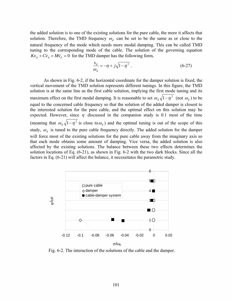
the added solution is to one of the existing solutions for the pure cable, the more it affects that solution. Therefore, the TMD frequency dω can be set to be the same as or close to the natural frequency of the mode which needs more modal damping. This can be called TMD

ning to the corresponding mode of the cable. The solution ovMvCKv &&& for the TMD damper has the following form,

tu f the governing equation 0=++ ddd

21 ηηω

−+−= js

As shown in Fig. 6-2, if the horizontal coordinate for the damper solution is fixed, the

vertical movement of the TMD solution represents different tunings. s f

d

d . (6-27)

In thi igure, the TMD solution is at the same line as the first cable solution, implying the first mode tuning and its maximum effect on the first modal damping. It is reasonable to set 21 ηω −d (not dω ) to be equal to the concerned cable frequency so that the solution of the added damper is closest to the interested solution for the p le, and the optimal effect on this solution may be expected. However, since

ure cabη discussed in the companion study is 0.1 most of the time

21 ηω −d is clo(meaning that se to dω ) and the optimal tuning is out of the scope of this study, dω is tuned to the pure cable frequency directly. The added solution fo per

axis so at each mode obtains some amount of damping. Vice versa, the add solu also

isting solutions. The balance between these two effects determwo dark blocks. Since all the

factors in Eq. (6-21) will affect the balance, it necessitates the parametric study.

ions of the cable

r the damwill force most of the existing solutions for the pure cable away from the imaginary th ed tion is affected by the ex ines the solution locations of Eq. (6-21), as shown in Fig. 6-2 with the t

Fig. 6-2. The interaction of the solut and the damper.

0

1

-0.12 -0.1 -0.08 -0.06 -0.04 -0.02 0 0.02

0

6

2

3

ϕ/ ω

0

4

5

σ/ω

pure cabledampercable- amper systemd

101

6.5 A Special Case for Transfer Function Analysis of Forced Vibrations

The performance of the TMD damper can be evaluated in terms of the reduction of the cable resonant response due to a forced vibration. As an example for the forced vibration analysis, an evenly distributed harmonic force with the form of t

yysexff ω)( j~

= is applied perpendicular to the cable chord to derive the transfer function. A small normalize le

distributed damping

d cab

0ωmcc = of 0.01 is chosen to avoid an infinite resonant response, which

corresponds to a distributed damping of 493.0=c N/m2. The TMD damper is placed at the mid-span since only placement of the mid-s n for the first mode tuning is discussed in this section.

the mid-span. The 2λ parameter is very small for this figure, rendering the fundamental

mode tuning implies

the dis pa

Fig. 6-3 shows the transfer function for the cable with and without the TMD damper at

natural frequency of the cable very close to that of a taut cable, which indicates that the first

110

===c

ddω

ωω

ωρ . The response cv is tted in a logarithmic

scale. The first peak, also the largest one, for the pure cable corresponds to a resonant frequency at

plo

rad, which is close to the fundam le natural frequency ental cab 1cω01.64=sω . The TMD is tuned to the first mode with a frequency of 01.641 == cd ωω rad. Therefore, two peaks appear in the transfer function curve for the cable-damper system around the first natural frequency of the pure cable due to mode splitting, as expected. The smaller one is

38.580 =ω rad and the larger one is 30.691 =ω rad. Though the TMD causes a little larger response on both sides, it reduces the resonant response of the pure cable significantly. The cable peak displacement with a TMD is only 9.12% of that without a TMD. An optimal tuning, defined as the lowest ratio of the maximum response with a damper to that without a damper, will give a ratio of 7.19% at a frequency ratio of 96.0=ρ . This is reasonable, as Den Hartog (1956) pointed out that the optimal tuning for a single degree-of-freedom structure with a TMD damper is )1/(1 rm+=ρ . However, for simplicity, the TMD damper is tuned to the fun

ns

6.6 Conclusions A linear theory on free and forced vibration pro

small sag attached with a discrete Tuned Mass Damper (TMD) is proposed through an analytic

damental cable frequency, which provides the damper performance close to the optimal tuning. Since the mass ratio is small at large, this approach is adequate for the comparison purpose. The third modal response is also reduced (with a 49% peak response of that for the pure cable), though not as effective as for the first mode. Another thing worthy to be pointed out is that there is no peak respo e at the second cable natural frequency since the even number modes (antisymmetric ones) are not excited under the evenly distributed force.

blems of a planar inclined cable with a

al approach in this study. The proposed equations include parameters such as cable geometry-elasticity parameter, cable internal damping, cable inclination, damper position, mass, stiffness, and damping ratio. The free vibration problem becomes an eigenvalue

102

problem, whose solution includes the information of the modal frequency and damping for the cable-TMD system. The installation of TMD affects the system char in a w to add one more solution to the governing equations and thus changes of the solution locations for the pure cable. The displacement response for a harmonic force is also readily obtained, and the effectiveness of the TMD damper is investigated and verified by a case study through a transfer function analysis. The application of the derived equations on an experimental cable will be present companion study via a parametric approach. The formulations to determi the cable response to an arbitrary force, such as wind-rain excitation, is more difficult and requires further investigation.

acteristics ay

ed in the ne

.7 Notations

-1

6 A : The area of the cable cross section c : The normalized cable distributed damping

:d The sag of the mid-span of an inclined cable E : The Young’s modulus of the cable

xf , yf : The distributed cable force along the x and y directions, respectively g : The gravitational acceleration

h : dsdxh τ=

H : The constant horizontal component of tension force the cable

40 60 80 100 120 140 160 180 200-4

-3.5

-3

-2.5

-2

-1.5

ωs (rad)

log(

v c) (m

)

cable-TMD system

pure cable

Fig. 6-3. Transfer function of the cable with and without TMD damper.

103

1−=j : The imaginary root K , C , M : The spring, damping coefficient, and mass for the TMD-MR damper, respectively

le mass and damping coefficienween the TMD and the

ex variableation

1l , 2l , l : The chord length for the left segment, right segment, and the whole cable, respectively

eL : The effective cable length m , c : The distributed cab t per unit length, respectively

rm : The mass ratio bet cable

1r , 2r : The normalized length for each segment, respectively s : The compl representing the vibration characteristics

ds : The eigenvalue solution of the damper governing equs′ , s′ : The Lagrangian coordinate in the unstrained and strained cable profile t : The time T , τ : The nsion, respstatic and dynamic cable te ectively u , v : The cable dynamic displacement components along the x and y coordinates, respectively

1v , 2v : The displacements of the cable for the corresponding segments

cv , dv : The cable displacement where the TMD damper is located and the damper displacement that is along the perpendicular direction to the cable chord, respectively

1x , 2x , x : The ordinate for the left segment, right segment, and the whole cable, respectively

β : The complex variable defined by Hcsms )cos()( 2 θβ +

±=

β ′ : The variable defined by lββ 5.0=′ ε : The ratio of the cable weight to the tension force η , dω : The damping ratio and the annular natural frequency for the damper, respectively

2λ : The cable geometry-elasticity parameter θ : The inclined cable angle measured from the horizontal axis ρ : The frequency ratio of the damper to a taut cable

: The ratio of the force frequency to the taut cable frequency 'ρ

iσ , iϕ : The real part and imaginary part of the solution of the basic equation for the i-th mode, respectively

is

: The fundamental angular frequency for a taut cable 0ω: The natural frequency for the pure cable ciω

iω , iζ : The damped frequency and the modal damping for the i-th mode of the cable-damper system, respectively

)()(od

d • : The derivative of “ ” with respect to “ ” • o

)()(o∂•∂ : The partial derivative of “ ” with respect to “ ”

• o

104

6. 8 Re

Wu, W.J. and Cai, C.S. (2005) “Cable vibration control with a TMD-MR damper system:

Theoretical formulation and parametric study.” Proceedings of McMat2005, 2005 joint ASME/ASCE/SES Conference (CD), June 1-3, 2005, Baton Rouge, Louisiana, USA.

Triantafyllou, M.S. (1984) “The Dynamics o d cables.” Quarterly Journal of ics and Applied Mathematics, Vol. 27, NO.3, Aug., 1984, pp.421-440.

W ble vibration reduction with a hung-on TMD system: and Control (submitted)

ferences Cai, C.S., Wu, W.J. and Araujo, M. (2005) “Cable Vibration Control with a TMD-MR

Damper System: Experimental Exploration.” Proceedings of McMat2005, 2005 joint ASME/ASCE/SES Conference (CD), June 1-3, 2005, Baton Rouge, Louisiana, USA.

Chen, Z.Q., Wang, X. Y., Ko, J. M., Ni, Y.Q., Spencer, B.F., and Yang, G. Q. (2003). "MR

damping system on Dongting Lake cable-stayed bridge." Smart Systems and Nondestructive Evaluation for Civil Infrastructures, San Diego, California, USA, 2-6

Tabatabai, H.， Mehrabi, A.B. (1999) “Tuned Dampers and Cable Fillers for Suppression of

Bridge Stay Cable Vibrations.” IDEA program final report, Construction Technology Laboratories, Inc., Skokie, IL.

March 20.

Den Hartog, J.P. (1956) "Mechanical Vibrations." 4th Edition, McGraw-Hill, NY.

Irvine, H.M. and Caughey, T.K. (1974) “The linear theory of free vibrations of a suspended cable.” Proceedings of Royal Society (London), A341, 299-315.

Johnson, E. A., Christenson, R. E., and Spencer, B. F. Jr. (2003) "Semiactive Damping of Cables with Sag." Computer-aided Civil and Infrastructure Engineering, 18, 2003, 132-146.

Li, W. H., Yao, G. Z., Chen, G., Yeo, S. H. and Yap, F. F. (2000). "Testing and Steady State Modelling of a Linear MR Damper under Sinusoidal Loading." Smart Materials and Structures, Vol. 9, 95-102.

Pacheco, B.M., Fujino, Y., and Sulekh, A. (1993). "Estimation curve for modal damping in stay cables with viscous damper." Journal of Structural Engineering., 119(6), 1961-1979.

f Taut inclineMechan

u, W. J. and Cai, C. S. (2006) “Ca

parametric study.” Journal of Vibration

105

106

Yu, Z. and Xu, Y. L. (1998). "Mitigation of three dimensional vibration of inclined sag cable using discrete oil dampers-I. formulation." Journal of Sound and Vibration, Vol. 214(4), 659-673

Xu f inclined sag cable using

d application." Journal of Sound and Vibration, Vol. 214(4), 75

, Y. L. and Yu, Z. (1998). "Mitigation of three dimensional oiscrete oil dampers-II.

6 -693, 1998

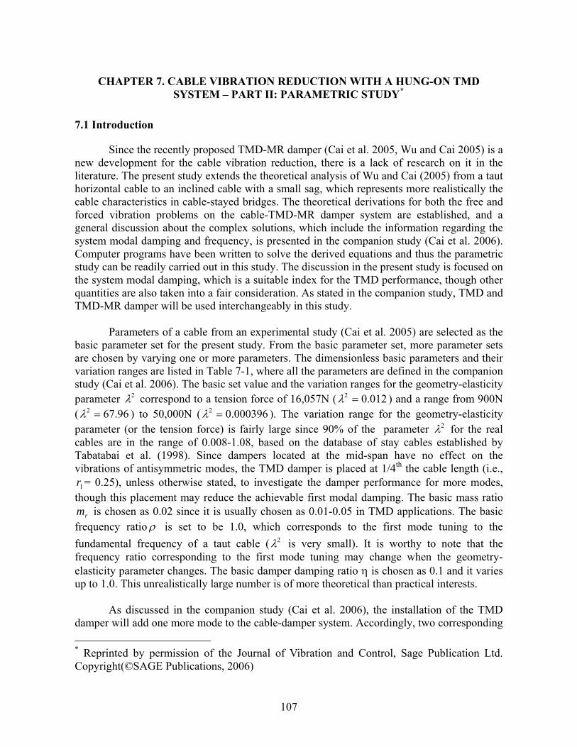
CHAPTER 7. CAB E VIBRATION REDUCTION WITH A HUNG-SYSTEM – PART II: PARAME

L ON TMD TRIC STUDY*

7.1 Introduction

Since the recently proposed TMD-MR damper (Cai et al. 2005, Wu and Cai 2005) is a t for the cable vibration reduction, there is a lack of research on it in the

terature. The present study extends the theoretical analysis of Wu and Cai (2005) from a taut

cable cforced

eneral discussion about the complex solutions, which include the information regarding the

Compustudy cthe sys amping, which is a suitable index for the TMD performance, though other

uantities are also taken into a fair consideration. As stated in the companion study, TMD and

basic p more parameter sets re chosen by varying one or more parameters. The dimensionless basic parameters and their

study (parame respond to a tension force of 16,057N ( ) and a range from 900N

cables abatab ampers located at the mi

., s,

though this placement may reduce the achievable first modal damping. The basic mass ratio is chosen as 0.02 since it is usually chosen as 0.01-0.05 in TMD applications. The basic

new developmenlihorizontal cable to an inclined cable with a small sag, which represents more realistically the

haracteristics in cable-stayed bridges. The theoretical derivations for both the free and vibration problems on the cable-TMD-MR damper system are established, and a

gsystem modal damping and frequency, is presented in the companion study (Cai et al. 2006).

ter programs have been written to solve the derived equations and thus the parametric an be readily carried out in this study. The discussion in the present study is focused on tem modal d

qTMD-MR damper will be used interchangeably in this study.

Parameters of a cable from an experimental study (Cai et al. 2005) are selected as the arameter set for the present study. From the basic parameter set,

avariation ranges are listed in Table 7-1, where all the parameters are defined in the companion

Cai et al. 2006). The basic set value and the variation ranges for the geometry-elasticity ter 2λ cor 012.02 =λ

( 96.67 ) to 50,000N ( 000396.0 ). The variation range for the geometry-elasticity parameter (or the tension force) is fairly large since 90% of the parameter 2λ for the real

are in the range of 0.008-1.08, based on the database of stay cables established by ai et al. (1998). Since d

2 =λ 2 =λ

T d-span have no effect on the vibrations of antisymmetric modes, the TMD damper is placed at 1/4th the cable length (i.er = 0.25), unless otherwise stated, to investigate the damper performance for more mode1

rmfrequency ratio ρ is set to be 1.0, which corresponds to the first mode tuning to the

ental frequency of a taut cable ( 2λ is very small). It is worthy to note that the cy ratio corresponding to the first mode tuning may change when the geometry-

fundamfrequen

ticity parameter changes. The basic damper damping ratio η is chosen as 0.1 and it varies p to 1.0. This unrealistically large number is of more theoretical than practical interests.

damper cable-damper system. Accordingly, two corresponding

elasu

As discussed in the companion study (Cai et al. 2006), the installation of the TMD will add one more mode to the

Copyri* Reprinted by permission of the Journal of Vibration and Control, Sage Publication Ltd.

ght(©SAGE Publications, 2006)

107

solutions will appear around that of the mode of the pure cable (without damper) where the

thereaf orresponding to the rger amplitude of vv

TMD frequency is tuned to. The added mode, called zero-th mode or damper related mode ter for the convenience of descriptions, is defined as the one c

la cd /~ ~ (damper displacement over cable displacement at the damper

importa

Table 7-1. Basic parameter set and the parameter variation range*

position), which can be obtained from the two solutions, though the two solutions have equal nce when a cable mode is in tune.

2λ θ (°) 1r rm ρ η

Basic Parameter

Set 0.012 11.27 0.25 0.02 1 0.1

Parameter Variation

Range

0.0004~ 68 0~60 0.01~0.5 0.008~0.20 0.1~5 0.01~1

* : The variation range may change slightly in some discussions.

.2 System Modal Damping Analysis In this section, emphasis is placed on the achievable maximum modal damping ratio.

or simplicity, as discussed earlier, the TMD damper is always tuned to the cable’s ental natural frequency, except as otherwise stated.

.2.1 Effect of Cable Geometry-elasticity Parameter ( ) Irvine (1981) predicted that the nth frequency crossover occurs when the cable

eometry-elasticity parameter reaches for a horizontal cable. Triantafyllou (1984) eld the opinion that a frequency avoidance replaces the frequency crossover when the eometry-elasticity parameter is equal to for an inclined cable. The parabolic static

ay be one of the reasons that cause a frequency crossover instead of the equency avoidance observed in the current study. However, this will not affect the iscussion on the system damping very much (especially for small inclinations) since it still aptures the symmetric and antisymmetric exchange of modes. Xu and Yu (1998) pointed out at the first system modal damping provided by an oil damper installed near the cable pport may be dramatically affected by the cable geometry-elasticity parameter (They

sag parameter in their paper). In their paper, for an oil damper located at 2% of e cable length from the cable end with a sag parameter ranging from 8 to 40, the achievable aximum first modal damping ratio was 60% less than that for cables with a sag parameter

1 (can be viewed as a taut cable). These cables are usually long cables with latively small tension forces, most of which actually need more damping.

Fig. 7-1(a) shows the relationship between the system modal damping ζ and the cable

eometry-elasticity parameter with the TMD damper located at 1/4th the cable length for

7

Ffundam

2λ7

2λ 2)2( nπgh

2λ 2)2( nπgcable profile used mfrdcth

2λsucalled it thethmless than 0.re

2λg

108

an inclined cable with a basic parameter set (Table 7-1). The modal damping for the damper relat is considered, including ). In Fig. 7-1(a),

, actually only the zeroth mode and the first two modes are affected this is a first mode tuning. The curves in Fig. 7-1(a) can be separated into

two pa

ed mode and the first five cable related modes are plotted. A wide range of λ the first frequency crossover point ( )2( 22 ≈= πλ

2

40with the increase ofdramatically since

2λ

rts according to the values of λ . When 40≤λ , with the increase of λ , the zeroth modal damping keeps reducing, the first modal damping increases then reduces within a limited level, and the second modal damping keeps increasing. When 402 ≥λ , with the increase of 2λ , the zeroth modal damping keeps increasing, the first modal damping increases a little bit then remains constant, and the second modal damping keeps reducing. When the 2λ is close to 40, the zeroth and first modal damping are close to the minimum values, while the second modal damping is around the maximum value.

These observations can be explained with the frequency relation between the pure

cable and the cable-TMD system, as shown in Fig. 7-1(b). When 2λ is very small, there is a big difference between the first and the second frequencies for the pure cable. The first one is around 0

2 2 2

ω and the second one is around 02ω , where 0ω is the frequency of a corresponding taut cable. Since the TMD damper is tuned to the fundamental le frcab equency ( 01 ωω =c ), the firs

m value, wd sec modes are tuned at the same

ows some d ed to Fig. 7-1(a). In Fig. 7-2(a), when is less than about 30, only the first m dal damping gains a lot of damping. After is larger than 30, the first modal damping drops dramatically to almost zero, and the second modal damping jumps up and

t mode gains much more damping than other modes, and it seems that only the zeroth and the first mode share the total damping, as shown in Fig. 7-1(a). With the increase of 2λ , the frequency difference between the first two modes for the pure cable becomes small. Consequently, the TMD damper has more effect on the second mode, and the second modal damping becomes larger. When 2λ reaches 40 (the crossover value for the pure cable), the frequency difference of the pure cable reaches its minimu hich means that the first an ime. Therefore, the second modal damping for the cable-TMD system achieves its maximum value. Correspondingly, the zeroth and the first modal damping achieve their minimum values, and it seems that the damping for the zeroth mode and some part of the first modal damping have been transferred to the second mode. After that, the first two frequencies separate again, and the second modal damping for the cable-damper system reduces to a small value again. While crossover is observed for the first two modes of the pure cable near 2λ = 40, the installation of the TMD at 1/4th the cable length entails modification from frequency crossover to avoidance, since dampers placed there have a strong effect on the antisymmetric modes. For higher modes, the modal damping is small since their frequencies (not plotted in Fig. 7-1(b)) are far enough from the tuning frequency so that the effect of the TMD is small.

Fig. 7-2(a) shows the relation between the modal damping and the cable geometry-

elasticity parameter 2λ when the TMD damper is installed at the mid-span, which sh

ond t

ifference compar 2λ2λo

continues the track of the first modal damping. When 2λ is larger than the

109

frequen

ations in Fig. 7-2(a) can thus be explained with riantafyllou’s theory on the mode shapes of the inclin er at the mid-

span will hav l damping is always zero when is less than 30 (the crossover point of the cable-TMD system). At this point, the first mode becomes antisymmetric and the sec nd mode become ymmetric. Correspondingly, the first modal damping becomes zero and the second modal damping jumps up

C F , a TMD placed at the mid-span does improve the first modal

damping 0 t u Ho it after this his ab change can be overcome by placing the TMD damper at an

e TMD damper at 1/4th the able length in this study. Other results with different inclination angles (0º and 60 º) show

at /4th the cable length will change the original over to avoidance, while TMDs at mid-span will cause a backward shifting for

the freq

cy crossover point of pure cable ( 2λ =40), the zeroth modal damping increases and the second modal damping decreases.

Fig. 7-2(b) shows that when the TMD is installed at the mid-span, it entails a

backward shifting of the frequency crossover point from 402 =λ to 302 =λ , which is different from the observation made from Fig. 7-1(b), where the TMD causes the modification from the frequency crossover to avoidance, since dampers placed at the mid-span do not affect the antisymmetric modes. The observT ed cable. Since the damp

e no effect on the antisymmetric modal damping, the second moda2λ

o s s

abruptly.

ompared toby about 2point. T

ig. 7-1(a)% before

rupthe freq ency avoidance point. wever, reduces to zero

appropriate location. This is also one of the reasons to place thcsimilar observations that TMDs placed 1frequency cross

uency crossover point. 7.2.2 Effect of Cable Inclination (θ )

ab damper system was based on a able so that the effect of cable inclination on the modal damping could not be

investig damp

In the previous work (Wu and Cai 2005), the c le-horizontal taut c

ated. In this more refined cable model, the cable inclination effect is ready to be investigated, while its effect on the modal ing is found through the geometry-elasticity parameter 2λ and the frequency ratio ρ .

Fig. 7-3 shows the effect of cable inclination on the system modal damping with two

different cable tension forces. In Fig. 7-3(a), the tension force is large (T=16,057N) causing the geometry-elasticity parameter to be small ( 012.02 =λ ). Therefore, the zeroth modal damping and the first modal damping are much larger than the modal damping for other modes, which is close to zero. The modal damping remains almost constant as the cable inclination changes. However, in Fig. 7-3(b), the tension force (1,075N) is chosen to make the

2λ value at the first frequency crossover point correspond to an inclination of 11.27º. Therefore, the first and the second modal dampings are much larger than the other modal dampings when the inclination angle is less than 11.27º. At this time, both the first mode and the second mode are tuned. When the inclination is at 11.27º, the frequency avoidance occurs, the second modal damping reaches its maximum value, and the zeroth andamping reach their minimum values. When the inclination is larger than 11.27º, th

d the first modal e zeroth

110

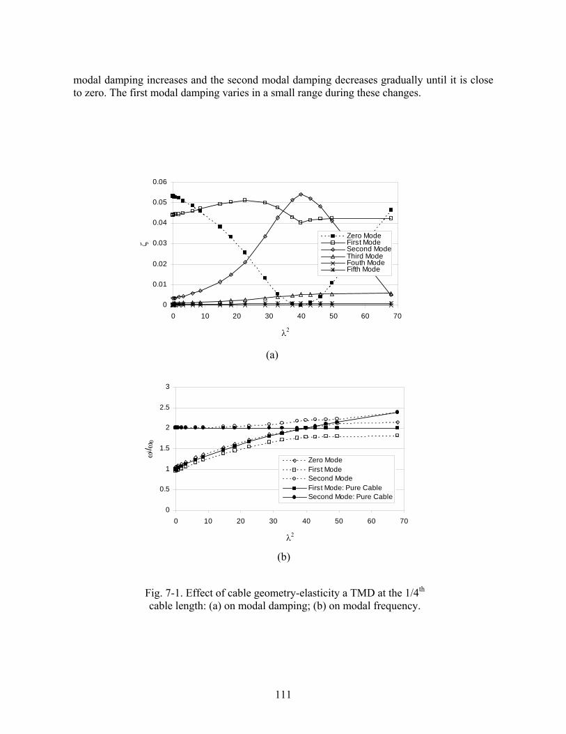
modal damping increases and the second modal damping decreases gradually until it is close to zero. The first modal damping varies in a small range during these changes.

(a)

0.02

0.03

0.04

0.05

0.06

ζ

Zero ModeFirst ModeSecond ModeThird ModeFouth Mode

0

0.01

0 10 20 30 40 50 60 70

λ

Fifth Mode

t

2

(b)

0

0.5

1

1.5

2

2.5

3

0 10 20 30 40 50 60 70

λ2

ωi/ ω

0

Zero ModeFirst ModeSecond ModeFirst Mode: Pure CableSecond Mode: Pure Cable

Fig. 7-1. Effect of cable geometry-elasticity a TMD at the 1/4 h cable length: (a) on modal damping; (b) on modal frequency.

111

0

0.

0 10 20 30 40 50 60 70

0.01

0.02

03

0.04

0.05

0.06

0.07

0.08ζ

Zero ModeFirst ModeSecond ModeThird ModeFouth ModeFifth Mode

λ2

(a)

2

2.5

3

1.5

Fig. 7-2. Effect of cable geometry-elasticity parameter with a TMD at the mid-span: (a) on modal damping; (b) on

modal frequency.

(b)

0

0.5

0 10 20 30 40 50 60 70

1

λ2

ω 0ωi

/

Zero ModeFirst ModeSecond ModeFirst Mode: Pure CableSecond Mode: Pure Cable

112

These observations in Fig. 7-3 can also be explained by the frequency tuning affected by the cable geometry-elasticity parameter 2λ . When the tension force is equal to 16,057N, the 2λ parameter is much less than the first frequency crossover point, despite the inclination change. Therefore, the first mode tuning of the TMD damper will not have much effect on the

o dam However, when the tension force is equal to ,075N, the parameter will be close to and finally less than the first frequency avoidance oint when the inclination angle increases (when the inclination angle increases, the value ecreases). Accordingly, the second modal damping achieves a high value when the first and cond frequencies are close, and then reduces back to zero when they separate.

Therefore, the cable inclination affects the modal damping mostly via the parameter

. Special concern should be put on the parameter when it passes the frequency rossover/avoidance point when the cable inclination changes. The results also indicate that hen the cable tension is large, i.e., when the is much smaller than that corresponding to e frequency crossover/avoidance, the inclined cable can be analyzed as a taut horizontal

able since the inclination effect is small in this case. Otherwise, the analysis of an inclined able is necessary for stay cables since the inclination may have significant effects on the able modal damping.

.2.3 Effect of Damper Position ) Due to the physical restriction, viscous dampers are usually installed near the cable

pport on the deck, which constraints the vibration mitigation effectiveness of the damper. oreover, Xu and Yu (1998) reported that the modal damping provided by oil dampers may

rop dramatically since the cable mode shape may be zero at a place close to the support hen the cable geometry-elasticity parameter is close to the frequency avoidance point. he TMD dampers can provide more freedom to improve the cable damping since they can be laced anywhere along the cable.

Fig. 7-4 shows the variation of the modal damping of the cable-damper system when

e damper is placed at different positions. From Fig. 7-4(a) we can see that when the TMD amper is placed at the end of the cable (say < 0.05), the damper related modal damping is rge and close to the damper damping ratio 0.1, and all the cable related modal damping are

lose to zero. This indicates that the TMD damping is not effective when it is installed near e cable end. When the damper is moved toward the mid-span, the damper related modal

amping reduces and the first modal damping increases until it arrives at . After that, e damper related modal damping increases and the first modal damping decreases until it

rrives at . From to

m1pdse

cwthccc 7

suMdwTp

thdlacthdtha

dal ping of the second or higher modes. 2λ

2λ

2λ 2λ

2λ

( 1r

2λ

1r

18.01 =r

35.01 =r 35.01 =r 40.01 =r , these two switch and keep almost constant ntil mid-span. For the modal damping associated with higher modes, they are small ompared to the zeroth and the first modal dampings since the TMD is tuned to the first cable ode.

ucm

113

0.06

0

0.01

0.02

0.03

0.04

0.05

0 10 20 30 40 50 60 70

Zero ModeFirst Mode

θ

ζ

Second ModeThird ModeFouth ModeFifth Mode

(a)

(b)

0

0.01

0.02

0.03

0.04

0.05

0.06

0 10 20 30 40 50 60 70

Zero Mode

θ

ζ

First ModeSecond ModeThird ModeFouth ModeFifth Mode

Fig. 7-3. Cable inclination effect on system modal damping with different tension force: (a) T=16,057N; (b) T=1,075N

114

When only the modal damping of higher modes is considered, interesting information an be observed in Fig. 7-4(b). For the i-th mode, there is a peak modal damping at

= ir

i

c2,3,1),2 ≥= nin L . After the peak, the modal damping reduces to zero and repeats.

The higher the mode, the more repeated times. This occurs because the cable points at 22,1,1 ≥== ninr L are actually the nodes of these modes. Therefore, any damper

located at these nodes will have no contribution to the i -th modal damping. The higher mode has more nodes, rendering more repeated times. It is also worthy to point out that when the TMD damper is constrained close to the support as 10.01

/(1

/

<r , the modal damping for the second to the fifth mode is very close. This observation is similar to that for viscous dampers (Xu and Yu 1998). 7.2.4 Effect of Mass Ratio ( )

er

m

atio up to 20% is numerically studied for a thorough understanding of e performance of the TMD-cable system. The damper stiffness has also been varied

t the first mode tuning.

r

The mass of a traditional TMD damp is important for its control effectiveness.

Generally speaking, the reduction effectiveness becomes better with a larger TMD mass ratio if the optimal tuning is achieved. However, the ass ratio is usually in the range of 1%-5% in practice since too large a TMD mass may cause many problems during construction and maintenance, as well as an increased cost. Therefore, considerations of the mass ratio should be included during the TMD damper design. In the present study, though a large mass ratio is not practical, the mass r

m

thaccordingly to meet the requiremen of

Displayed in Fig. 7-5(a) is the relationship between the system modal damping and the

mass ratio. With the increase of the mass ratio, the zeroth modal damping reduces monotonically. Meanwhile, the first modal damping increases from about 027.01 =ζ at

008.0=rm to a peak value about 0.044 at 0175.0=rm , and reduces to about 0.031 at 2.0=rm , and the second modal damping increases monotonically. All the other modal

damping for higher modes also increases monotonically, but by a much smaller value. By extending the trend of the curves for the zerot mp

elieve that the first modal damping approaches zero when the mass ratio

on stu ai et al

mass ratio and a larger mass ratio, at

h and the first modal da ing, we have enough reason to bapproaches zero. This can also be verified by investigating the basic equation, Eq. (6-21) in chapter 6. When the mass ratio rm approaches zero, the left hand side of the equation approaches zero, and the whole equation goes back to the governing equation for the free vibration of a pure cable. Therefore, every modal damping should be zero when the cable distributed damping is neglected. When the mass ratio increases, the trend of the curves for the modal damping can be explained with the frequency change in Fig. 7-5(b). With the increase of the mass ratio, the zeroth and the first frequencies separate and the tuning is away from the optimal tuning. As discussed in the transfer function analysis for the forced vibrations in the compani (C . 2006), while the second mode becomes relatively closer to the zeroth mode, it gains more damping and the first modal damping becomes less. Consequently, a maximum first modal damping appears somewhere between the zero

dy

0175.0=rm in this case. Therefore, increasing e mass ratio may not guarantee a better mitigation effect for the targeted mode. However, th

115

Fig. 7-5(a) does show that with the increase of more modes will gain their modal damping nd the overall mitigation effectiveness may be enhanced.

rma

Fig. 7-4. Damper position effect on system modal damping: (a) all modal damping; (b) only higher modal damping.

0

0.02

0.04

0.06

0.08

0.1

0.12

0 0.1 0.2 0.3 0.4 0.5 0.6

r1

ζZero ModeFirst ModeSecond ModeThird ModeFouth ModeFifth Mode

(a)

0

0.0005

0.001

0.0015

0.002

0.0025

0.003

0.0035

0.004

0 0.1 0.2 0.3 0.4 0.5 0.6

r1

ζ

Second ModeThird ModeFouth ModeFifth Mode

(b)

116

7.2.5 Effect of Frequency Ratio ( ρ )

performance, it is of great im

Since the tuning of the TMD damper to the cable will significantly affect the TMD

portance to know the relationship between the modal damping and the frequency ratio ρ (the ratio of the damper frequency to a taut cable frequency)

uation. As stated before, it is essential to design a damper stiffness to tune the damper frequency to the desired tuning frequency of the structure under control. An inappropriate stiffness of TMD dampers may significantly reduce the control effectiveness. However, it should be noted that since cable frequency is different from a taut cable frequency when 2λ is not very small, a first mode tuning may not imply the frequency ratio equal to 1.0.

considered in the basic e

the pure

ys modal damping versus the variation of the frequency ratio values. In Fig. 7-6(a), when the frequency ratio

q

Fig. 7-6 exhibits the s tem2λ ρwith two different is very small, the

damper related modal damping is almost the same as the damper damping ratio 0.1, and the first five cable related modal damping is almost zero. This observation indicates that the installation of the damper cannot effectively improve the cable modal damping with a small frequency ratio since it is out of tune. As the frequency ratio increases, the zeroth modal damping decreases and the modal damping of all the five modes increases, while their peak values appear in sequence. When the frequency ratio ρ is equal to 1.0, the TMD damper is actually tuned to the fundamental frequency of the real pure cable 1cω since with a small 2λ value of 0.012, 1cω is very close to the first natural frequency of a taut pure cable 0ω ( 00049.1/ 01 =ωωc ). Therefore, the first modal damp ng ratio is significantly improved, and

e zer

per is outune again.modes o

ith oth modal damping reduces significantly due to transferring the damping from the damper to the cable. After that, the first modal damping decreases, and the zeroth modal damping increases as if the damping goes back to the zeroth mode when the dam t of

With a further increase of the frequency ratio, the second mode and all the other f the pure cable are tuned and the corresponding modal damping reaches the

maximum value in sequence, except for the fourth modal damping, since the TMD damper is located at one of the nodes of the fourth mode.

When the geometry-elasticity parameter 2λ changes, similar observations can be

made, except that the maximum modal damping may appear at a different frequency ratio, as shown in Fig. 7-6(b). Since the first ( 1cω ) and the second ( 2cω ) natural frequencies of the pure cable are very close to each other with a geometry-elasticity parameter 88.392 =λ (avoidance point) and they are almost twice of the first natural frequency of a taut cable 0ω with the same tension force, the maximum first and second modal damping appears at 2=ρ at the same time. Meanwhile, the zeroth modal damping reduces to almost zero as if all the damping has been transferred to the first and the second modes. This observation indicates that there is a balance for the damping among all the modes, which will be discussed in detail later.

117

(a)

0.08

0

0.01

0.02

0.03

0.04

0.05

0.06

0.07

0.00 0.05 0.10 0.15 0.20

mr

ζ

Zero ModeFirst ModeSecond ModeThird ModeFouth ModeFifth Mode

Fig. 7-5. Damper mass effect on system modal damping: (a) modal damping versus mass ratio; (b) damped frequency versus mass ratio.

(b)

0

0.5

1

1.5

2

0 0.05 0.1 0.15 0.2

mr

ωi/ ω

0

Zero ModeFirst ModeSecond ModeFirst Mode: Pure CableSecond Mode: Pure Cable

118

7.2.6 Effect of Damper Damping Ratio (η )

odeled as an equivalent system consisting of a spring

KM , a dashpot with a damping coefficient C , and a mass M , the TMD damper actually has two functions. Firstly, it can transfer the cable vibration by the spring and the mass, which mainly depends on the frequency ratio discussed in the previous section. Secondly, it dissipates the vibration energy through the damping coefficient, which will be discussed in this section through the damper damping ratio.

Presented in Fig. 7-7 is the relationship between the system modal damping and the damping ratio of the TMD dampe with two different 2λ values. The variation range of the damper damping ratio consi

r dered is up to an impractical value of 1.0, which is more of

theoretic

od

al interests than practical implications. The zeroth modal damping is not plotted since its value is relatively too large to fit in the figures. When 2λ is very small, as shown in Fig. 7-7(a), all the five m al dampings increase with the increase of the damper damping ratio, especially the first modal damping. This indicates that the damper can provide more damping to the cable by increasing the damping ratio, and that the first mode will gain much more damping than other modes because of the first mode tuning. The first modal damping reaches the maximum value of 0.053 at 14.0=η . After that, the first modal damping reduces monotonically. The second modal damping begin to reduce after it reaches its maximum value of 0.013 at 7.0=η . Modal damping for higher modes is comparatively much smaller. The observation fits well with the common intuition. When the damp damping ratio is ve small, the TMD damper cannot dissipate the vibration energy effectively, rending a cabd th a low damping. When the damper damping ratio is very large, the dashpot impairs the movement of the spring and the TMD works as a rigid bar so that the vibration can not be transferred from the cable to the TMD effectively. This observation is also consistent with the discussion on the optimal damping ratio via the locations of the solutions in the companion study (Cai et al. 2006). For cables with other 2λ values, the observations are similar, and the optimal damper damping ratio for the first mode appears at the same places of 14.0=

er ryle-

amper system wi

η with different achievable modal damping. Therefore, an optimal damping ratio will not change for different cable geometry-elasticity parameters, if the mass ratio and the first tuning method are chosen. This observation may simplify the design of the damper

tigate

for different cables.

7.3 Higher Mode Tuning

In reality, not only the first cable mode but also the second or higher modes may be excited in a wind-rain induced cable vibration. Therefore, it is also important to inves the relationship between the modal damping and the damper damping ratio for a higher mode tuning.

119

0

0.02

0.04

0.06

0.08

0.1

0.12

0 1 2 3 4 5 6

ρ

ζZero ModeFirst ModeSecond ModeThird ModeFouth ModeFifth Mode

(a)

0

0.02

0.04

0.06

0.08

0.1

0.12

0 1 2 3 4 5 6

ρ

ζ

Zero ModeFirst ModeSecond ModeThird ModeFouth ModeFifth Mode

(b)

Fig. 7-6. Effect of frequency ratio on system modal damping: (a) 012.02 =λ ; (b) 88.392 =λ .

120

0

0.01

0.02

0.03

0 0.2 0.4 0.6 0.8 1

η

ζ

0.04

0.05

0.06

First ModeSecond ModeThird ModeFouth ModeFifth Mode

(b)

(a)

0

0.01

0.02

0.03

0.04

0.05

0.06

0.07

0 0.2 0.4 0.6 0.8 1

η

ζ

First ModeSecond ModeThird ModeFouth ModeFifth Mode

Fig. 7-7. Effect of damper damping ratio on system 2 2modal damping: (a) 012.0=λ ; (b) 19.6=λ .

121

Fig. 7-8 shows the relationship between the system modal damping and the damping ratio of the TMD damper with two different values using the second mode tuning. Compared to Fig. 7-7, there are two important changes for the modal damping curves. The first is that the second modal damping instead of irst modal damping is much larger than other m . The second is that there are two peaks instead of one peak in Fig. 7-8. A mo detailed investigation of the change in the solutions of the basic equations reveals that hen the damper damping increases to some value (

2λ

the fodal damping, as expected for a second mode tuning

rew

1.0=η in this case), the damping distribution changes between the zeroth mode and the second mode. Therefore, there is a modal damping drop for the second mode from 1.0=η to 12.0=η . After that, the modal damping curve for the second mode follows a similar trend, just like that for the first mode in Fig. 7-7. Another thing to note is that the change point and the optimal damping point will not change when the geometry-elasticity parameter changes, which is also similar to Fig. 7-7. 7.4 Energy Transfer and Damping Redistribution

From the energy point of view, the vibration reduction is to find a way to transfer and finally dissipate the vibration energy of structures under consideration. For a cable, the total vibration energy is composed of the vibration from each mode. If the cable vibration energy can be effectively transferred and dissipated by adding dampers, the cable vibration will be effectively reduced for sure. Since the modal damping is a direct indicator of the capacity to dissipate energy per vibration cycle, which can reflect both the TMD and MR functions as stated in Cai et al. (2005), it is naturally a good index to represent the energy transfer and dissipation. Correspondingly, the process of the cable vibration mitigation can be regarded as a process of a redistribution of the damping in TMD damper to each mode of the cable.

Previous figures show that wherever a peak of the cable related modal damping appears, there is a drop for the damper relat odal damping. However, the total modal damping for all modes seems to be the same. It s that the damping has been “transferred” from the zeroth mode (the damper related mode) to other modes (the cable related modes). This phenomenon is called damping redistribution in this paper. To discuss the distribution of the modal damping, the total modal damping is thus defined quantitatively as, ζ (7-1-a)

or ζ (7-1-b)

when only the first modal damping is counted in. Correspondingly, the relative error for the first modal damping with respect to the damper damping ratio can be defined as,

the

ed m seem

∑∞

==

0iit ζ

∑=

=n

ii

nt

0ζ

n n

η

ηζ −=

ntne (7-2)

122

where means the absolute value of •• . This quantity measures the relative accuracy of the hypothesis of damping redistribution, i.e., assum ng that the damper damping is distributed within the cable related modes and the damper related mode. and all the parameters considered in the previous sections. Figs. 7-9(a), (b), and (c) show a very small relative error when up to the first 5 modes are considered. Of igures, the maximum relative error is less than 3%, despite the variation of geometry-elasticity parameter, the inclination angle, and the damper position. Therefore, the damping redistribution hypothesis holds accurately for t e cases. However, in Fig. 7-9(d), the relative error increases almost proportionally when the mass ratio increases. This is because, as discussed earlier, as the mass ratio increases more damping will be distributed to higher modes. When the mass ratio

nei

n

Fig. 7-9 reveals the relationship between the relative error 5e

all the errors in the three f the cable

hes5e

, 2.0=rm , the maximum relative error reaches 17.3%.

However, the mass ratio used in real applications is commonly within the range of 0.01-0.05. In this range, the relative error is less than 5%, as shown in Fig. 7-9(d). Fig. 7-9(e) shows a very important point for the damping redistribution hypothesis. In Fig. 7-9(e), both the relative errors for the first ive modes and for the first eight modes are plotted. It seems that the relative error is too high to accept the damping redistribuhypothesis for a high frequency ratio, when only the first five modal dampings are considered. However, this observation reveals that the damping is redistributed to all modes, and thpreference of the redistribution depends on the tuning. For example, when the frequency ratio is equal to 1.0, the damping is mainly distributed to the first 5 modes, and thus e5 is smdiscussed. However, when the frequency ratio is equal to 5, which means the TMD damptuned to the fifth mode of a taut cable, not only itself and the lower modes such as mand 3, but also the higher modes such as m des 6 and 7, may gain a certain amount of damping. Therefore, when the modal damping of higher modes is counted, the relative error will be reduced greatly. As shown in Fig. 7-9(e), the error is much less than for the cases of high frequency ratios. Fig. 7-9(f) showwide range of damper damping ratios in the cases of both the first mode tuning and the second mode tuning. From the previous discussions, neither the cable properties, such as the geometry-elasticity parameter and the inclination angle, nor the damper properties, such as the damper position, the frequency ratio, the damper damping, nor the tuning method, will make the damping redistribution hypothesis invalid. The mass ratio does cause worse accuracy. However, in the application range of the mass ratio, the error is acceptable (less than 5%). Therefore, damping redistribution can be applied with fair accuracy for most cases. The fundamental reason for this damping redistribution should be energy conservation for the cable-damper system. However, this discussion the current study.

5e

5e

5e 8e tion

e

all as er is

odes 2

f

o

8e 5es that the damping redistribution is valid for a

is beyond the scope of

123

0.02

0.03

0.04

0.05

0.06

0.07ζ

First ModeSecond ModeThird ModeFouth ModeFifth Mode

0.01

00 0.2 0.4 0.6 0.8 1

η

(a)

0.05

0.06

First ModeSecond Mode

0

0.01

0.02

0.03ζ

0.04

0 0.2 0.4

η

Third ModeFouth ModeFifth Mode

0.6 0.8 1 1.2

(b)

Fig. 7-8. Effect of damper damping ratio on system modal damping with second mode tuning: (a) 012.02 =λ ; (b) 19.62 =λ .

124

0.03

0

0.005

0.01

0.015

0.02

0.025

0 10 20 30 40 50 60 70

λ

θ=11.27

θ=60

2

e5

(a) Cable geometry-elasticity parameter

0.005

0.01

0.015

0.02

0.025

e5

T=16057N

T=1075N

0

0 10 20 30 40 50 60 70

θ

(b) Cable inclination

Fig. 7-9. Damping redistribution with different parameter variation: (a) cable geometry-elasticity parameter; (b) cable inclination; (c) damper position; (d) mass

ratio; (e) frequency ratio; (f) damper damping ratio.

125

(c) Damper position

0

0.005

0.01

0.015

0.02

0 0.1 0.2 0.3 0.4 0.5

0.025

0.03

r1

e5

λ2=0.012λ2=6.19

(d) Mass ratio

0 0.02 0.04 0.06 0.08 0.1

0.12 0.14 0.16 0.18 0.2

0 0.05 0.1 0.15 0.2 mr

e 5

λ2=0.012λ2=6.19

Fig. 7-9. Cont’d

126

(e) Frequency ratio

0 0.05

0.1 0.15

0.2

0.25 0.3

0.35 0.4

0 1 2 3 4 5

ρ

e

λ2=0.012, e5

λ2=6.19, e5

λ2=0.012, e8

λ2=6.19, e8

0

0.01

0.02

0.03

0.04

0.05

0.06

0 0.2 0.4 0.6 0.8 1 η

e5

λ2=0.012, 1st mode tuning λ2=6.19, 1st mode tuning λ2=0.012, 2nd mode tuning λ2=6.19, 2nd mode tuning

(f) Damper damping ratio

Fig. 7-9. Cont’d

127

7.5 Co

e lutions of the basic equations derived in the companion paper (Cai et al. 2006). Parameters ch as the cable geometry-elasticity parameter, the cable inclination, the damper position, the ass ratio, the frequency ratio, and the damper damping ratio are considered. Comparing the tal modal damping of the cable-damper system and the damping ratio of the damper reveals e rule of damping redistribution from the damper to each mode of the cable-damper system.

The modal damping is significantly affected by the geometry-elasticity parameter in

e sense that the change of the geometry-elasticity parameter may change the cable equency, which may cause the TMD damper to tune to two cable frequencies near the equency crossover/avoidance point at the same time. The effect of the TMD on the first ode exchanges with that of the second mode when the geometry-elasticity parameter

xceeds the frequency crossover point when the damper is placed near the mid-span. owever, this can be overcome by placing the TMD damper near the 1/4th point of the cable ngth where only the frequency avoidance is observed.

If the geometry-elasticity parameter is much less than that corresponding to the

equency crossover/avoidance, which corresponds to a large cable tension force, the effect of able inclination on modal damping is small, implying that in this case the stay cables can be nalyzed as a horizontal taut cable.

An increase mass ratio does not necessary improve the modal damping of the targeted

ode. However, it does increase the modal damping of higher modes. There exists an optimal damper damping for the cable-TMD system. While too small a

amper damping is not sufficient in dissipating vibration energy, one too large will lock the ibration of the damper, which is not beneficial in transferring vibration from the cable to the amper.

The damper position and frequency ratio will affect the distribution of damper

amping to different modes. These parameters need to be chosen carefully for a targeted ode (or targeted modes). Multiple TMDs may be warranted to target more modes since the

ominating mode vibration may not be clear during the damper design process. This study is of considerable practical interest since it can be applicable to a traditional

MD damper or the TMD-MR damper that has proven to be a promising way to increase the able-damper system damping (Cai et al. 2005, Wu and Cai 2005).

.6 References

ai, C.S., Wu, W.J. and Araujo, M. (2005) “Cable Vibration Control with a TMD-MR Damper System: Experimental Exploration.” Proceedings of McMat2005, 2005 joint ASME/ASCE/SES Conference (CD), June 1-3, 2005, Baton Rouge, Louisiana, USA.

nclusions A parametric study has been carried out to investigate the parameter influence on th

sosumtoth

thfrfrmeHle

frca

m

dvd

dmd

Tc

7 C

128

Cai, C

vine, H.M. (1981) “Cable Structure.” MIT Press Series in Structural Mechanics, Cambridge, Massachusetts, and London, England, 1981.

u, W.J. and Cai, C.S. (2005) “Cable vibration control with a TMD-MR damper system: Theoretical formulation and parametric study.” Proceedings of McMat2005, 2005 joint ASME/ASCE/SES Conference (CD), June 1-3, 2005, Baton Rouge, Louisiana, USA.

abatabai, H.， Mehrabi, A.B.， Morgan, B.J., and Lotfi, H.R. (1998) “Non-destructive Bridge Technology: Bridge Stay Cable Condition Assessment.” Final report submitted to the Federal Highway Administration, Construction Technology Laboratories, Inc., Skokie, IL.

riantafyllou, M.S. (1984) “The Dynamics of Taut inclined cables.” Quarterly Journal of Mechanics and Applied Mathematics, Vol. 27, NO.3, Aug., 1984, pp.421-440

u, Y. L. and Yu, Z. (1998). "Mitigation of three dimensional of inclined sag cable using discrete oil dampers-II. application." Journal of Sound and Vibration, Vol. 214(4), 675-693, 1998

. S., Wu, W. J. and Shi, X. M. (2006) “Cable vibration reduction with a hung-on TMDsystem: theoretical study.” Journal of Vibration and Control (Accepted)

Ir

W

T

T

X

129

CHAPTER 8. COMPARISON BETWEEN VISCOUS DAMPER AND TMD-MR DAMPER ON CABLE VIBRATION REDUCTION

are susceptible to external disturbances such as vortex shedding, rain-wind induced vibration, vehicle

Johnson et al. 2003). As a method of semiactive control, MR dampers have recently been used because of their advantages over other

itions are restricted at the cable ends. To further improve the effectiveness on cable vibration reduction, Tuned Mass Dampers (TMD) dampers was propose

99). The effectiveness of TMD dampers depends on the tuning to the cable vibration frequency, which indicates that TMD d

frequency is difficult to be predicted due to various uncertainties. Wu and Cai (2006) conducted a parametric study on the modal damping of the cable-TMD-MR system and dis

pplication conditions for these two types of dampers. The current study is trying to provide some information on this

and Yu (1998) pointed that the out-of-plane vibration of a cable with and ithout viscous dampers performs the same as a taut cable, a comparison is focused on the

modal

8.1 Introduction As key load-carrying members of cable-stayed bridges, stay cables are of primary

importance to secure the safety of the entire structure. Since cables are generally flexible, relatively light, and low energy-dissipative because of their inadequate intrinsic damping, they

-induced vibration, and other excitations due to parametric disturbances caused by the motion of either the bridge deck or towers.

To suppress the problematic vibrations, a common practice is to install mechanical

(including viscous/oil and Magnetorheological (MR)) dampers, with one end connected to the deck and the other end connected to the cable, at a distance typically 2-5% of the cable span length from the lower end. A large research effort has been exerted on viscous/oil dampers (Pacheco et al. 1993, Yu and Xu 1998, Xu and Yu 1998,

traditional mechanical dampers, such as their adjustable large damping force, mechanical simplicity, reliability, and minimum power requirement (Chen et al. 2003). However, as Cai et al. (2005) pointed out, the traditional mechanical dampers might not be the most effective because their pos

d, which can be placed anywhere along the cables to overcome the shortcomings of position restriction of mechanical dampers (Tabatabai and Mehrabi 19

ampers with self-adjusting function on its own frequency, such as a TMD-MR damper (Cai et al. 2005) or other TMD dampers with variable stiffness, will have a broader implementation potential than regular TMD dampers in a complicated system where the cable vibration

cussed the influence of the parameters such as the cable geometry-elasticity parameter, the cable inclination, the damper position, the mass ratio, the frequency ratio, the damper damping ratio, or the tuning mode on the effectiveness of the TMD damper, represented by the system modal damping.

Up till now, a comprehensive comparison between the effectiveness of the TMD and

the viscous damper with the same cable configuration is not available in the literature; such a comparison would aid in the deeper understanding of the suitable a

point. Since Xu wperformance of the planar in-plane vibration in this study in terms of transfer functions and

damping.

130

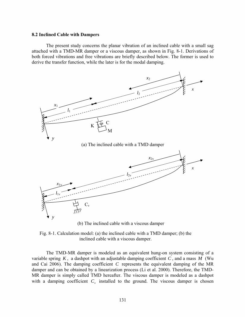
8.2 Inclined Cable with Dampers The present study concerns the planar vibration of an inclined cable with a small sag

both fo ibed below. The former is used to erive the transfer function, while the later is for the modal damping.

The TMD-MR damper is modeled as an equivalent hung-on system consisting of a

variable spring

attached with a TMD-MR damper or a viscous damper, as shown in Fig. 8-1. Derivations of rced vibrations and free vibrations are briefly descr

d

K , a dashpot with an adjustable damping coefficient , and a mass C M (Wu and Cai 2006). The damping coefficient represents the equivalent damping of the MR damper and can be obtained by a lineariz nMR damper is simply called TMD hereafter. he viscous damper is modeled as a dashpot with a damping coefficient installed to the ground. The viscous damper is chosen

Catio process (Li et al. 2000). Therefore, the TMD-

TvC

Fig. 8-1. Calculation model: (a) the inclined cable with a TMD damper; (b) the inclined cable with a v cous damper. is

(a) The inclined cable with a TMD damper

l1

l2

K C

My

x

x1

x2

(b) The inclined cable with a viscous damper

l1v

l2v

Cv

y

x

x1v

x2v

131

per D damper is also plac 1, the existence of

e damper divides the cable into two segments, with the length indicated in the figure. The bscript will be used to represent either segment and applicable for systems

with different dampers. The x coordinate is taken as along the cable chord direction, and the y coordin

he detailed derivation of an inclined cable with a small sag attached with a TMD damper

pendicular to the cable chord as it is believed to be the optimal placement. The TMed perpendicular to the cable chord. As shown in Fig. 8-

thnotation without su

ate is perpendicular to the x coordinate and in the downward direction. The left support of the cable is taken as the origin of the Cartesian coordinate system for the first segment and the right support as the origin for the second segment. The notation of the cable-viscous damper system is similar to that of the cable-TMD damper system, with a subscription of ‘v’ to indicate the viscous damper.

T can be found in Cai et al. (2006). The derivation of an inclined cable with a small sag

installed with a viscous damper can be found in Yu and Xu (1998) in a different approach. However, the important equations and the derivation are summarized here for the purpose of narrative and comparison. The equation of motion for the cable segment can be expressed as

tvc

tvm

xdydh

xvHf y ∂

∂+

∂∂

=+∂∂

+ 2

2

2

2

2

2

cosθ (8-1)

where yf is the distributed cable force along the y direction; H is the constant horizontal component of the cable tension force; θ is the inclined cable angle measured from the horizontal axis; v is the cable dynamic displacement components along the y coordinate measured from the static equilibrium position of the cable; m and c are the distributed cable mass and damping coefficient per unit length, respectively; and t is the time. The notation

)()(od

d • denotes the derivative of “ • ” with respect to “ o ” and )()(o∂•∂ means the partial derivative

of “ • ” with respect to “ o ”.

A parabolic static profile is chosen by neglecting higher orders of a small quantity

1)cos( <<= θεH

mgl , the ratio of the cable weight to the tension force. The inequality implies

that the tension force in the cable is large compared to its weight so that the sag and the slope of the cable are small.

The elastic deformation caused by the cable vibration generates a secondary tension

force, which in turn causes additional deformation. By examining the relation between the strain and the stress of a small element, the compatibility equation can thus be obtained as

∫=+l

vdxlHEAh

0

22 cos)cos811(

cosθεθε

θ (8-2)

where E is the Young’s modulus of the cable; A is the area of the cable cross section; and h is defined as the component of the dynamic tension force along the x ordinate.

132

The cable equation can be analytically solved for some external loadings with a special form, such as an evenly distributed force in the form of exff )( st

yy~

= , leading to the following solution

)1)sinh(

))sinh()(sinh()(

)cos(~~(

)sinh()sinh(~)(~

2 −+−−

−=k

ky

kck l

xxll

hlflxvxv

βββ

βθε

ββ , 2,1=k (8-3)

where the complex variable s can be viewed as an angular frequency, which represents the vibration characteristics; cv is the cable displacement where the damper is located; and β is

defined as Hcsms )cos()( 2 θ+ for narrative simplicity. Terms with a tilde represent that they

are functions of the position variable only.

The existence of the damper provides a force boundary condition for the cable point where the damper is placed. As for the viscous damper, the boundary condition leads

t

vC

xv

xvH c

v

lx

v

lx

v

vv

∂∂

=∂∂

−∂∂

−==

)(cos

2211

2

2

1

1

θ (8-4)

For the TMD damper, the boundary condition leads

)()()(cos

1111

2211

11

2

2

1

1

dtdv

dtdvCvvK

xv

xvH d

lxdlx

lxlx

−+−=∂∂

−∂∂

−=

=

==θ

(8-5)

The installation of the TMD actually adds one more degree of freedom to the cable-

damper system, or called modal splitting. Therefore, one more equation, meaningly, the equilibrium of the damper itself should be counted in, as

0)()( 2

21

111

11=−−+−

== dt

vdMdt

dvdtdvCvvK dd

lxdlx

(8-6)

With further derivation from the previous simultaneous equations, the eigenvalue

equation governing the free vibration problem of the cable-viscous damper system can be obtained from Eqs. (2)-(4) as ( 0~

=yf ),

)}4)(cosh()){sinh(sinh(

)}4)(cosh()cosh()){sinh(sinh()sinh(4

32

322121

βλ

ββββ

βλ

ββββββπξ

′+′′−′′−=

′+′′′−′′′ vvvv rrrr (8-7)

where notations llr vv /11 = , llr vv /22 = , lββ 5.0=′ , and )2/( 0ωξ mlCv= are defined.

lmH π

θω

cos0 = is the fundamental angular frequency for a taut cable, and 2λ is

proportional to the ratio of the cable axial stiffness to the cable geometry stiffness (and thus called the cable geometry-elast ty parameter hereafter): ici

133

θθε

θελcos/cos

811

1)(cos22

222

HAE

+= (8-8)

Similarly, the governing equation for the free vibration problem of the cable-TMD damper system can be obtained from Eqs. (2), (3), (5), and (6) as ( 0~

=yf ),

)}4)(cosh()){sinh(sinh()}4

)){sinh(sinh()sinh()/'(4)/'(4

)/'(44

3

2122

2

βββπβπβηρρ

πβηρρβ ′′′++

+′ rrmr(8-9)

)(cosh()cosh( 3β2221 λβββββ

λβββ ′+′′−′′−=′+′′′− rr

where mlMmr = is the mass ratio between the TMD and the cable and ρ is the frequency

ratio of the TMD to a taut cable and will be referred to as the frequency ratio.

The simultaneous equations for the cable-viscous damper system on the forced ibration problem with an evenly distributed force in the formv of st

yy exff )(~= are listed

below, which can be obtained from Eqs. (2), (3), (5), and (6).

)2/cosh()2/cosh()2/sinh(cos~

)2/cosh()2/cosh()sinh(cos 2/~

))sinh()sinh(

)sinh(2(~

212

212

2

21

rrHf

rrlHh

rrv

y

c

βββ

βθ

βββ

βθε

βββπξ

′′′

×=

′′′

×+′′

′+

(8-10-a)

))2/cosh()2/cosh(

)2/sinh(2(cos

)

)2/cosh()2/cosh(/

~

)2sinh(2(cos~

)2/~

212

2

ββθβ

βββ

β

−′

=−

′′′

′′

f

rrlHrv

y

c

(8-10-b)

Similarly, th

cosh()2/cosh()2/sinh(

3

2

1

βθεββ

β−+

′×

hr

2122 βββλ ′′ rrH

e equations for the forced vibration of the cable-TMD damper system can be found in Cai et al. (2006), or simply by changing the term πξ2 in Eq. (10-a) to the corresponding term for the TMD damper.

8.3 Com

le-damper system for a free vibration is no doubt a proper criterion, which indicates the damper capacity to dissipate energy in each vibration circle. The first fivinto consideration. Since the installation of the TMD damper adds one more degree of

m le

ined as damper related mode or the zeroth mode. They have equal importance for the cable-TMD damper system.) (Wu and Cai 2006).

parison on Achievable System Modal Damping

To evaluate the performance of a damper, the achievable modal damping of the cab

e modal dampings are taken

freedom to the cable-damper system (i.e., one ode splits into two modes), only the cab related mode is compared (defined as the one with the smaller value of the ratio of TMD amplitude to the cable amplitude at the damper location. The other mode is def

134

Several cables with different geometry-elasticity parameters are considered since the damper performance may change for different cables. Those cables are chosen according to the 2λ values as far less than (0.012, as a taut cable), less than (6.19), close to (39.88), and large than (49.54) the first frequency crossover point (Irvine 1981). Though a better performance of the viscous damper can be observ tion m ves toward the mid-span, two damper locations, and from the lower cable end, are considered to

r 48.39)2( 2 =πed when its loca o

l02.0 l05.0reveal a thorough variation of the system damping influenced by the geometry-elasticity parameter 2λ , the damper location vr1 , and the damping ratio ξ . The mass ratio rm for the

TMD damp chosen as 1/ 1

cable-TMD damper system is chosen as 0.02, as commonly used in practice. The tuning of the

to the cable is er =cd ωω , where the dω and 1cω are the damper frequency and the cable fundamental freque

ncy, respectively.

Fig. 8-2 displays the relation between the damping ratio and the modal damping for the cab

checo’s results (Pacheco et al. 993). Fig. 8-2(a) show odal damping curve, which implies that for a cable with a small value (or very largwhen the modal damping is plotted against the multiplication of the damper damping ratio

le-viscous damper for four cables with different 2λ values stated previously with the damper placed at l02.0 from the cable end. Figs. 8-2(a) and 8-2(b) are similar to Pa

1 s the so-called universal m2λ e tension force in the cable),

ξ , the mo the curves for the first five modes are very close. Fig. 8-2(b) shows that when the value increases, the curve for the first

odal damping lowers down. However, the other four modal damping curves do not change. With a further increase of the value, when it is a little larger than the first frequency crossover point, several modal damping curves alter considerably, as shown in Fig. 8-2(c). The fir

urther increase of the value to 49.54, the second modal damping curve begins to rise, the third modal damping curve lowers

own more, and the other curves remain without noticeable change.

ig. 8-3 shows the change of the modal damping curves affected by the geometry-elastici

odal damping level of a taut cable, and remains unchanged afterwards. In Fig. 8-3(b) the second modal damping curve stays unvaried before the value

aches t rst frequency crossover point, becomes zero at the crossover po o creases when the value increases further. In Fig. 8-3(c) the third moda e

continues to decrease when the value increases. In Fig. 8-3(d) the fourth modal damping y when th value changes in the red range. Thes

can be explained with the mode exchange rule occurred at the frequency crossover point. Irvine (1981) poimodes exchange. As Xu and Yu (1998) pointed out, the modal shape ordinate of the first

de number i, and the normalized damper location r1v, 2λ

m2λ

st modal damping curve ascends back to the same level as in Fig. 8-2(a) with the optimal damping ratio shifting left. The second modal damping curve becomes close to zero and the third modal damping curve drops down. With a f 2λ

d

Fty parameter for each mode. In Fig. 8-3(a) the first modal damping curve decreases

when the 2λ value increases before it reaches the first frequency crossover point, comes back almost to the equal optimal m

2λre int, and begins tin l damping curv

he fi2λ

2λcurve does not var e conside e observations

nted out that at the first frequency crossover point, the first and second

symmetric mode close to cable end entails for the cable a very small motion over there before

2λ

135

th amping. However, after the c elated properties exchange

e frequency crossover, and thus causes a small first modal drossover, the mode exchange occurs and all the mode-r

accordingly. Therefore, the descending first modal damping curve rises back to the original eight and the unmoved second modal damping curve drops dramatically at that point. Since e

hth value considered is far below the second frequency crossover point, the fourth modal damping curve is not influenced.

2λ

(a) λ2=0.012

0

0.00

0.01

0.012

0 0.05 0.1 0.15 0.2 0.25 0.3 0

ξ i r1

006

8

Mode 10.ζ

Mode 2Mode 3Mode 4Mode 5

0.002

0.004

.35

r1v

(b) λ2=6.19

00 0.05 0.1 0.15 0.2 0.25 0.3 0.35

ξ i r1

0.008

0.01

0.012Mode 1Mode 2Mode 3Mode 4Mode 5

0.004

0.006ζ

0.002

r1v

Fig. 8-2. Variations of modal damping with the damping ratio of a viscous damper for four cables: (a) λ2=0.012; (b) λ2=6.19; (c) λ2=39.88; (d) λ2=49.54.

136

Fig. 8-2. Cont’d

(c) λ2=39.88

00 0.05 0.1 0.15 0.2 0 5 0.3 0.35

ξ i r1

0.002

0.004

0. 06

0.008

0.01

0.012ζ 0

.2

Mode 1Mode 2Mode 3Mode 4Mode 5

r1v

(d) λ2=49.54

0

0.002

0 0.05 0.1 0.15 0.2 0.25 0.3 0.35

ξ i r1

0.006

0.008

0.01

0.012

ζ

Mode 1Mode 2Mode 3Mode 4Mode 5

0.004

r1v

137

138

(b) The second mode

0

0.002

0.004

0.006

0.008

0.01

0.012

0 0.1 0.2 0.3 0.4 0.5 0.6 0.7

ξ i r1

ζ

16057, mode 22000, mode 21075, mode 21000, mode 2

λ2=0.012 λ2=6.19 λ2=39.88 λ2=49.54

r1v

(a) The first mode

0

0.002

0.004

0.006

0.008

0.01

0.012

16057

0 0.05 0.1 0.15 0.2 0.25 0.3 0.35

ξ i r1

ζ

200010751000

2=0.012 λ2=6.19 λ2=39.88 λ2=49.54 λ

r1v

Fig. 8-3. Variations of modal damping with the cable geometry-elasticity parameters: (a) the first mode; (b) the second mode; (c) the third mode; (d) the fourth mode.

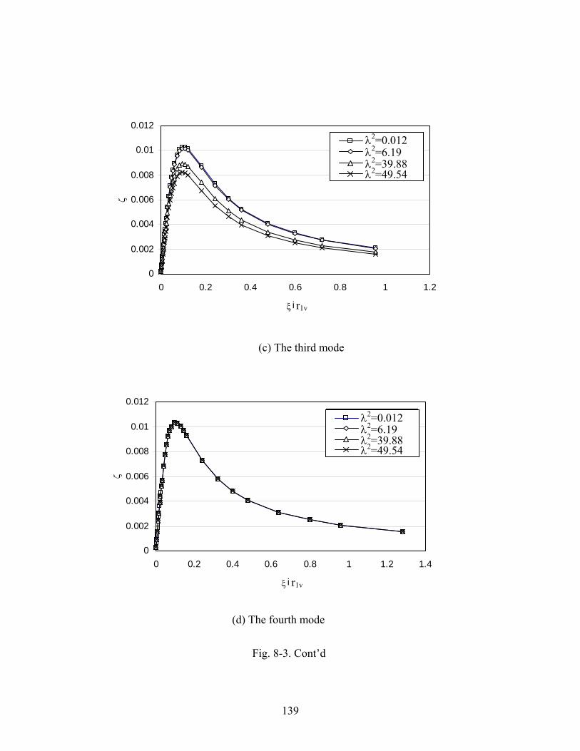
0

0.002

0.004

0.006

0.008

0.01

0.012

0 0.2 0.4 0.6 0.8 1 1.2

ξ i r1

ζ

16057, mode 32000, mode 3

Fig. 8-3. Cont’d

(c) The third mode

1075, mode 31000, mode 3

2=0.012 λ2=6.19 λ2=39.88 λ

λ2=49.54

r1v

0

0.002

0.004

0.006

0.008

0.01

0.012

0 0.2 0.4 0.6 0.8 1 1.2 1.4

ξ i r1

ζ

16057, mode 42000, mode 4

(d) The fourth mode

1075, mode 41000, mode 4

λ2=0.012 λ2=6.19

2=39.88 λ λ2=49.54

r1v

139

Presented in Fig. 8-4 is the variation of the modal damping versus the damper amping ratio for a cable with a value equal to 0.012 and a damper located at the om the cable end. Compared to Fig. 8-2(a), the maximum modal damping in Fig. 8-4

nd the higher modes attain larger optimal modal damping while they overlap each other and us have the same optimal modal damping as a universal modal damping curve in Fig. 8-

(a). Therefore, the universal modal damping curve is only eligible for the design of a viscous amper located very close to the cable support to mitigate the vibration for a cable with a

all value. The comparison results for the damper located at and for cables ith other values are similar and therefore are not shown here.

Fig. 8-5 plots the relation between the damping ratio and the modal damping for the

able-TMD damper system for four cables with different values stated previously with a amper placed at of the cable length. The modal damping curve for the damper lated mode is not plotted because it can not fit in the figure. Unlike Fig. 8-2(a), all five

urves separate from each other in Fig. 8-5(a). The peak modal damping for the first mode chieved by the TMD damper is almost 5 times of that achieved by the viscous damper, as own in Fig. 8-2(a). Actually, the TMD damper can provide a better system damping to the

able-damper system over a large range of the damper damping ratio

2λ l05.0 dfrincreases almost proportionally to the normalized location. However, the five curves separate ath2d

2λ l02.0 l05.0sm 2λw

0

0.005

0.01

0.015

0.02

0.025

0.03

0.035

0 0.05 0.1 0.15 0.2 0.25 0.3 0.35

ξ i r1

ζ

Mode 1Mode 2 Mode 3

Mode 4Mode 5

r1v

Fig. 8-4. The modal damping for a viscous damper at r1=0.05 with λ2=0.012.

2λcd 25.01 =rrecashc η than the maximum

amping provided by a viscous damper located at from the cable end. Even the modal amping of the second mode for the cable-TMD system is larger than the maximum damping f the cable-viscous system in Fig. 8-2(a) for a considerable range. However, the peak modal

d l02.0do

140

damping for the cable-viscous damper system is less sensitive in terms of the damper oefficient compared to the cable-TMD damper system in Fig. 8-5(a). The half-value

and (or their roportional counterparts) are the damper coefficients on either side of the damper coefficient orresponding to the peak modal damping at which the amplitude (the corresponding modal amping

cb aC bCandwidth of the damper coefficient is defined for this comparison. If pc

) is half of the peak modal damping, then the magnitude of the term ab CC −d ζ is efined as the half-value bandwidth of the damper coefficient. This concept can be used to heck the sensitivity of the optimal damper damping coefficient. The half-value bandwidth alculated from the first modal damping curve for the viscous damper is about 11288 N.s/m, hile it is 2.26 N.s/m for the TMD damper. This indicates that though the TMD damper can rovide better performance, it needs a more accurate design.

When the value increases, the peak modal damping of the cable-TMD system for

e first mode increases, as shown in Fig. 8-5, while that of the cable-viscous damper system ecreases before the value reaches the first frequency crossover point and returns to the itial damping level after the value passes the first frequency crossover point, as shown in ig. 8-3(a). The half-value bandwidth of the first modal damping curve for the cable-TMD stem increases from 2.26 N.s/m with a value of 0.012 to 4.37 N.s/m with a value of

9.88, as shown in Fig. 8-5(c). However, the half-value bandwidth for the cable-viscous amper system decreases from 11288 N.s/m to 5855 N.s/m, as shown in Fig. 8-3(a).

Fig. 8-5(c) also shows the effect of the mode exchange on the system damping. When

e TMD damping ratio reaches a certain value (0.1 in this case), mode exchange occurs etween the second and zeroth. After the mode exchange, the second modal damping ecomes zero, while the zeroth modal damping continues the track for the second mode. This ccurs since the installation of the TMD damper will affect the cable frequency to a fair egree. At the vicinity of the frequency crossover point, there is a complex interaction etween the first two frequencies of the cable and the damper frequency with the first mode

ng. They are so close that either two of them may exchange. More complicated mode xchange occurs in Fig. 8-5(d). Therefore, cables with value close to the frequency rossover point are not recommended. In this range, neither the viscous damper nor the TMD amper can guarantee a good performance in a predictable way. Actually, 90% of the stay ables have a value in the range of 0.008-1.08 based on the database of stay cables stablished by Tabatabai et al. (1998), which are far away from the crossover point

=39.48). The third system damping curve increases slowly when the value increases and is

uch lower compared to the first two damping curves. The fourth system damping curve is lways zero since the 1/4th point is a node for the fourth mode.

dccwp

2λth

2λd2λin

F2λ 2λsy

3d

thbbodbtuni

2λecd

2λce

2λ(

2λma

141

142

(a) λ2=0.012

0

0.01

0.03

0.04

0.05

0.06

ζFirst ModeSecond ModeThird ModeFouth ModeFifth Mode

0.02

0 0.2 0.4 0.6 0.8 1

η

0

0.01

0.02

0.03

0.04

0.05

0.06

0.07

ζ

First Mode Second Mode Third Mode

Fouth Mode Fifth Mode

0 0.2 0.4 0.6 0.8 1

η

(b) λ2=6.19

Fig. 8-5. Variations of modal damping with the damping ratio o a TMD-MR damper for four cables: (a) λ2=0.012; (b) λ2 19; (c) λ2=39.88; (d) λ2=49.54.

f=6.

0.02

0.03

0.04

0.05

0.06

0.07

0.08ζ

First ModeSecond ModeThird ModeFouth ModeFifth Mode

0

0.01

0 0.2 0.4 0.6 0.8 1

η

(c) λ2=39.88

0

0

0.02

0.03

0.04

0.05

0.06

0.07

0.08

ζ

.01

0 0.2 0.4 0.6 0.8 1

η

First ModeSecond ModeThird ModeFouth ModeFifth Mode

(d) λ2=49.54

Fig. 8-5. Cont’d

143

8.4 Comparison on Transfer Function

ibrations), the reduction of the cable resonant response to forced vibrations is also vestigated. In the current study, the first modal vibration is chosen as the target to be itigated, which means that if more reduction for the first modal vibration is achieved by

arying parameters of one damper, this damper is considered the better one. Since cables with eometry-elasticity parameters close to and larger than the frequency crossover point are not commended as discussed earlier, only two cables with values less than the first equency crossover point are considered in this section. A small distributed damping for the able of 0.493 N.s/m2 is chosen for the pure cable without dampers to avoid the infinite sonant response.

Xu and Yu (1998) (also by comparing Fig. 8-2(a) and Fig. 8-4 in this paper) pointed

ut that a viscous damper provides more achievable damping for the cable-damper system for e first five modes when the damper location moves toward the mid-span. The damper cation considered in their study is up to from the lower cable end, which is beyond the plementation restriction and more of theoretical interest. Therefore, the optimal location in

e current study for a viscous damper is selected as , perhaps the furthest realistic istance in applications. The viscous damper that can provide optimal modal damping for a ee vibration in the previous section is considered the initial optimal viscous damper for the rced vibration reduction and may be replaced if a better one is found after a search step of

.01 for the damper damping ratio in its vicinity. For the TMD damper, the optimal tuning equency is obtained by a trial-and-error process with a 0.01 step length of the tuning ratio he TMD frequency to the fundamental cable frequency

To evaluate the performance of the dampers, in addition to the modal damping (free

vinmvg

2λrefrcre

othlo l10.0imth l05.0dfrfo0fr(t 1/ cd ωω ), and so is the damper

amping ratio d η . The mass ratio of the TMD damper to the cable is chosen as 0.02. Two ifferent TMD damper locations are chosen due to the following reasons. The mid-span is hosen because the optimal system damping for the first mode is achieved there. The 1/4th able length is chosen because TMD dampers placed there are effective not only for the first odal damping but also for other modal damping.

Fig. 8-6(a) shows the transfer function for the pure cable and the cable with dampers

r a cable with a value of 0.012. There is no peak response associated with the second able mode in this figure since it cannot be excited by the evenly distributed force. The ptimal damper damping ratio for the viscous damper is

dccm

2λfoc

15.0=ξo and a reduction ratio of that is defined as the ratio of the displacement at the middle point of the cable

ith the damper to that without the damper. The optimal reduction ratio for the cable-TMD amper system is achieved as

185.0=redrw

0776.0=redrd with a tuning ratio of 96.0/ 1 =cd ωω and a damper amping ratio of 15.0=ηd . In this case the two supposed peaks for the cable-TMD damper stem are close, and thus appear like one with a boarder range. Therefore, the optimal

ibration by installing the TMD damper is another 58.1% less than that by using the viscous amper. For the third mode, the viscous damper provides a much better reduction than the MD damper since only the first mode is targeted for the TMD tuning. The comparison for

syvdT

144

the TMD damper at 1/4th of the cable length and the viscous damper is similar and is shown in

Fig. 8-5(b). Data for both cases are summarized in table 8-1 for reference.

Fig. 8-6. Transfer function comparison: (a) TMD damper at midspan; (b) er at 1/4th cable lenTMD damp gth

(b) TMD damper at 1/4th cable length

0.5 1 1.5 2 2.5 3-4

-3.5

-3

-2.5

-2

-1.5

-1

-0.5

0

0.5

1

ωs/ωc1

log(

v max

)

pure cablecable-TMDcable-viscous

0.5 1 1.5 2 2.5 3-4

-3.5

-3

-2.5

-2

-1.5

-1

-0.5

0

0.5

1

ωs/ωc1

log(

v max

)

pure cablecable-TMDcable-viscous

(a) TMD damper at midspan

145

The comparison results for the cable with a value of 6.19 are similar to that with a value of 0.012, which can also be found in table 8-1.

2λ2λ

Table 8-1. Comparison of cable vibration reduction between viscous damper and TMD

damper for the first mode

TMD Viscous damper

Cable TMD location Damping

ratio (η )

Tuning frequency

(1c

d

ωω )

Optimal reduction

( redr )

Damping ratio (ξ )

Optimal reduction

( redr )

midspan 0.15 0.96 0.0776 λ2=0.012 1.05 0.185 1/4th 0.15 1 0.1495

midspan 0.17 0.96 0.0677 λ2=6.19 1/4th 0.15 1.01 0.1259 0.85 0.2936

8.5 Comparison of Damper Design

The design of viscous dampers for a taut cable with a universal damping curve was

proposed by Pacheco et al. (1993). A similar approach of a TMD damper design for cables can be found in Wu and Cai (2006). A brief summary and comparison between designs for these two dampers for a taut cable are introduced here for demonstration purposes, based on the example used by Wu and Cai (2006). The intrinsic cable damping is conservatively ignored and additional damping is needed to suppress rain-wind induced vibrations. Other cable properties are listed in table 8-2. Damper designs for cables with large 2λ values need more information and effort, but can follow the same procedure.

Table 8-2. Properties of example cable

m (kg· -1) l (m) T (N) m p (kg/m3) D (m) (sec-1) 1cω114.09 93 5.017*106 1.29 0.225 7.08

Irwin proposed the following criterion to control the rain-wind induced cable vibration

αζ≥= 2pD

mSc (8-11)

where cS is the Scruton number; p is the mass density of air; D is the outside diameter of the cable; and α is the limiting cruton number. The onship can be rewritten as

value for S above relati

μααζ =≥

mpD 2

(8-12)

146

where the mass parameter μ is defined as )( 2pDm=μ . Therefore, to meet the above stated criterion, the damping ratio of the cable needs to meet the requirement of Eq. (8-12). Bas d on eavailable test results, Irwin proposed a minimum α of 10.

Since the mass parameter μ can be calculated as 1747)( 2 == pDmμ , the demanded modal damping is determined from Eq. (8-12) as %57.00057.01747101 ===≥ μαζ (8-13) 8.5.1 Design of Viscous Dampers

To design a viscous damper located at , the damper coefficient of the viscous

damper can be designed using Fig. 8-2(a). Based on this figure, values of

l02.0vir1ξ from 0.032

to 0.32 (from that the ξ can be calculated) will satisfy Eq. (8-13) and the corresponding damper coefficient is calculated as ξξ *08.7*93*09.114*22 0 == mlwCv =240388 to 2403885 N.s/m (8-14)Or the optimal damper coefficient is obtained as 901457 N.s/m that falls in the feasible range. 8.5.2 Design of TMD Dampers

Suppose the damper is placed at the 1/4th cable length. The mass ratio of the TMD-MR

damper is chosen as 2%, as in common practice, from which the mass of the dam er is determined as

p

kgmLM 2.21209.114*93*02.0**%2 === (8-15) The tuning ratio is then chosen approximately as 0.1/ 1 =cd ωω for simplicity, though

the optimal tuning may achieve a little better damping. The stiffness of the TMD-MR damper can therefore be determined as

mNmT

LMK /2.10648)

09.11410*017.5

9314159.3(*2.212)( 2

62 ===

π (8-16)

where mT

Lcπω =1

referred to and values of

is the fundamental frequency for a taut cable. Then Fig. 8-5(a) can be

83.0012.0 to=η can be chosen to satisfy Eq. (8-13) with an optimal damping ratio at 0.14, which corresponds to a damper coefficient of 420.7 N.s/m.

From the procedure stated above, the design effort is similar for these two dampers.

8.6 Conclusions

A comparison study between the characteristics of the cable-viscous damper system

and the cable-TMD damper system is presented through an analytical approach. From this study, the following conclusions can be drawn.

147

1. Thepa tems. For the cable-viscous damper system crease of the value f small to larger than the first frequency cro ps

l right afte e crossover point. At the same me, the peak modal damping for the second mode becomes zero and begins to increase

afterward. The peak modal damping for t ode reduces much for the fourth mode a emains unchang the For the cable- per sy he p al r o s e odal damping curve m the dam er-re al n at ency crossover point and beyond the point. The curve for the third mode is relatively uch lower a es the p . The f odal g is alw inced ocate node for the fourth m . 2 omparison conditio een a s dam ted at from

ith optimal damper damping ratio and a TMD damper located at 1/4 cable length or mid- tuning, and optimal damper damping ratio, the TMD

the targeted first mode, needs less damper dampin

o.

Further research ma e multiple TMD dampers to reduce the cable vibratio vibration less than that of the cab cous dam . 8.7 References

Pachecstay cables with viscous damper." Journal of Structural Engineering., 119(6), 1961-1979.

3

and Yu, Z. (1998). "Mitigation of three dimdiscrete oil dampers-II. application." Journal of Sound and Vibration, Vol. 214(4), 675-693.

system modal damping curve changes according to the cable geometry-elasticity rameter 2λ and the mode for both cable-damper sys

, with the in 2λ romssover point 24π , the peak modal damping for the first mode reduces to zero and po

r the 2λ value is beyond thback to thti

e initial leve

he third m slower, and thatlmost r

eak moday exchange with

ed during the first m

p

process.de becomelated mod

TMD damsecond mthe frequ

m

stem, t damping fo larger. Thdampi g

nd increasamper is l

slowly in rocess ourth m dampin ays zero s the TMD d at a ode

. At the c n betw viscou per loca l05.0 the cable end thw

span with a 0.02 mass ratio, optimaldamper can provide better vibration reduction to

g, and needs a more accurate design since its reduction effect is more sensitive to the damper damping. However, the viscous damper is effective for more modes at the same time, while the TMD damper is more focused to the targeted mode. It may need multiple TMD dampers to reduce vibration for several modes. 3. The designs to mitigate the rain-wind induced cable vibration by a viscous damper and a TMD damper are similar. All the damper parameters can be obtained acc rding to the demanded modal damping calculated based on the Scruton number requirement

y be carried out on the effectiveness of thn with a strategy to make all the modal

le-vis per system

o, B.M., Fujino, Y., and Sulekh, A. (1993). "Estimation curve for modal damping in

Yu, Z. and Xu, Y. L. (1998). "Mitigation of three dimensional vibration of inclined sag cable

using discrete oil dampers-I. formulation." Journal of Sound and Vibration, Vol. 214(4), 659-67

Xu, Y. L. ensional of inclined sag cable using

148

Johnson, E. A., Christenso , R. E., and Sp Jr. (2003) "Semiactive Damping of Cables with Sag." Computer-aided Civil and Infrastructure Engineering, 18, 2003, 132-146.

n encer, B. F.

.F., and Yang, G. Qed bridge." Smart

ructures, San Diego, California, USA, 2-6 March 20.

M. (2005) “Cable Vibration Control with a TMD-MR Damper System: Experimental Exploration.” Proceedings of McMat2005, 2005 joint ASME/ASCE/SES Conference (CD), June 1-3,

.” IDEA program final report, Construction Technology Laboratories, Inc., Skokie, IL.

f Vibration and Control (accepted).

Li, W.

ai, C. S., Wu, W. J. and Shi, X. M. (2006) “Cable vibration reducsystem

n, England, 1981.

abatabai, H., Mehrabi, A.B., Morgan, B.J., and Lotfi, H.R. (1998) “Non-destructive Bridge Technology: Bridge Stay Cable Condition Assessment.” Final report submitted to the

Chen, Z.Q., Wang, X. Y., Ko, J. M., Ni, Y.Q., Spencer, B . (2003). "MR

damping system on Dongting Lake cable-stay Systems and Nondestructive Evaluation for Civil Infrast

Cai, C.S., Wu, W.J. and Araujo,

2005, Baton Rouge, Louisiana, USA. Tabatabai, H., Mehrabi, A.B. (1999) “Tuned Dampers and Cable Fillers for Suppression of

Bridge Stay Cable Vibrations

u, W. J. and Cai, C. S. (2006) “Cable vibration reduction with a hung-on TMD system: W

parametric study.” Journal o

H., Yao, G. Z., Chen, G., Yeo, S. H. and Yap, F. F. (2000). "Testing and Steady State Modelling of a Linear MR Damper under Sinusoidal Loading." Smart Materials and Structures, Vol. 9, 95-102.

C tion with a hung-on TMD

: theoretical study.” Journal of Vibration and Control (accepted).

Irvine, H.M. (1981) “Cable Structure.” MIT Press Series in Structural Mechanics, Cambridge, Massachusetts, and Londo

T

Federal Highway Administration, Construction Technology Laboratories, Inc., Skokie, IL.

149

CHAPTER 9. CONCLUSIONS AND RECOMMENDATIONS

In this dissertation, in addition to using an existing MR damper, a new type of damper, a Tuned Mass D er-Magnetorheological (TMD-MR) damper is proposed and investigated theoretically and experimentally for cable vibration reduction. Comparisons on the reduction effectiveness between the proposed TMD-MR damper and other traditional dampers are carried out. The advantages and possible shortcomings of the proposed damper are addressed. This research work indicates that the proposed damper is practically implementable. 9.1 Experimental Study on Existing Individual MR Damper

First, experiments on the MR damper are carried out to gain some experience on the damper itself and the particular properties of the MR fluids. Experiment data shows that MR dampers can provide considerable damping

amp

forces under different loading conditions,

20°C and 30°C.

or nonzero

d, and the simulation research serves as a necessary step to n and implementation of the controller. Through a different experimental assive and semiactive experiments demonstrate that MR dampers are a good

an ophe s n current. MR dampers can help reduce cable vibrations under a variety of

activeay be too large for the cable vibration, which may deteriorate the control effect.

including different electric currents, loading frequencies, loading waves, and working temperatures. MR dampers can provide considerable damping forces even at their passive mode (with zero current) and have a large dynamic range. The damper used in this study has a maximum damping output force of 10N at the passive mode and about 80 N at the maximum current 0.5A, corresponding to a dynamic range of about 8. MR dampers can provide approximately the same damping force for a range of frequencies from 0.5Hz to 5Hz. The displacement-force curve shows that the energy that the MR dampers can dissipate is large when the loading wave is smooth. The working temperature does have some effect on the performance of MR dampers, especially between

To study the adjustability of the MR dampers, they are installed on the cable to reduce the cable vibration for both free and forced vibration through passive and semiactive control strategies. A passive control strategy implies the current is preset (either zerocurrent) and kept constant during the experiment, and the semiactive strategy implies the current is changing all the time, indicated by the control command based on the control algorithm. To utilize the Linear Quardratic Gaussian (LQG) algorithm, the control-oriented state-space equations are establisheguide the desigsetup, both the pchoice to reduce the cable vibration. The experiment with the passive MR damper shows that the reduction efficiency generally increases with the increase in the current. However, there is

timal current, beyond which the reduction effect will be the same. This current is called aturatiot

excitation frequencies and are most efficient for the resonant vibrations. Semiactive control experiments shows that the output force of the semiactive damper should be set around the

demand to achieve the best control effect. Otherwise, the damper output damping force m

150

9.2 Experimental Study on Proposed TMD-MR Damper

Bas

ed on the obtained information and experience, a TMD-MR damper was designed nd manufactured according to the vibration level of the experimental cable. The designed

effecthat tvibra pers. In addition, the installation of the TMD-MR damper also changed

e natural frequency of the cable-damper system. Extraordinary vibration reduction

to thaeffec en

e excitation frequency was not close to the cable natural frequency, the MR component

set inthus deteriorated the damping effectiveness. When the excitation frequency was close to the able natural frequency, the TMD component contributed mainly to track the excitation

energ the MR damper makes e TMD-MR damper system adaptable.

9.3 N

To get a profound and extended understanding of the TMD-MR damper performance,

estab ontal profile to aster the essentials of the cable-damper system and easily compare with research results on

better e analytical formula turned out to be an igenvalue problem for a free cable vibration with complex solutions. Discussions on the

criteras nomode

Based on the derived formula, thorough investigation of the effect of the cable/damper

parameters on the modal damping is carried out, including the cable geometry-elasticity parameter, the cable inclination, the damper position, the mass ratio, the frequency ratio, and the damper damping ratio. A higher mode t ng strategy is also considered. The modal damping is significantly affected by the geom try-elasticity parameter in the sense that the change of the geometry-elasticity parameter m y change the cable frequency of symmetric modes, which may cause the TMD damper to tune to two cable frequencies near the frequency crossover/avoidance point at the sa e time. However, this negative effect can be reduced by placing the TMD damper near the /4th point of the cable length where only the frequency avoidance is observed. If the geom -elasticity parameter is much less than that

aTMD-MR damper is then added to the cable, and possible factors that may affect the

tiveness of the TMD-MR damper are then investigated experimentally. It was observed he cable resonant vibration was considerably reduced down to 20%~30% of the cable tion without dam

thefficiency was achieved when the natural frequency of the TMD-MR damper was tuned close

t of the cable. After being tuned correctly, the TMD-MR damper is expected to be more tive for a wider range of different excitation frequencies than a traditional TMD. Wh

thcontributed mainly in providing an additional damping, and the TMD-MR should have been

the passive mode. A large current in the MR damper tended to lock the MR shaft and

cfrequency and transfer vibration energy to the damper, and the MR component worked as an

y dissipater to help reduce the cable vibration. The addition ofth

umerical Study on TMD-MR Damper

a simple, and then a more refined analytical model of the cable-TMD-MR system is lished. The simple one chooses the simple cable model with a horiz

mother types of dampers. The refined model considered an inclined cable with small sag, which

represented most stay cables in reality. Thedynamic characteristics of the established system, therefore, are focused on the performance

ia as the system modal damping achieved by the TMD-MR damper. Special cases such noscillatory decaying vibration and nondecaying oscillation are discussed in the simple l.

uniea

m1

etry

151

that correspo large cable tension force, the effect of cable inclination on odal damping is small, implying that in this

requency tio will affect the distribution of damper damping to different modes. These parameters

es).

cused to the targeted mode, dicating a multi-TMD system may be needed in applications.

adjustable assive MR damper. The final blueprint should be an adaptive semiactive MR damper. This eans a TMD-MR damper system should be integrated with a sensor, controller, and the MR

amper itself. The built-in sensor measures the vibration information from the cable, the easured information is analyzed, and the control signal is sent out by the controller to make

nding to the frequency crossover/avoidance, which corresponds to a m

case the stay cables can be analyzed as a horizontal taut cable. An increase of the mass ratio does not necessarily improve the modal damping of the targeted mode. However, it does increase the modal damping of higher modes. There exists an optimal damper damping for the cable-TMD system. While too small a damper damping is not sufficient in dissipating vibration energy, one too large will lock the vibration of the damper, which is not beneficial in transferring vibration from the cable to the damper. The damper position and franeed to be carefully chosen for a targeted mode (or targeted mod

Comparison studies are carried out between the viscous damper and the TMD-MR damper subsequently through a similar theoretical approach. Research results show that the system modal damping curve changes according to the cable geometry-elasticity parameter

2λ and the mode for the combined cable-damper systems. At the comparison condition between a viscous damper located at l05.0 from the cable end with an optimal damper damping ratio and a TMD damper located at 1/4th the cable length or on at the mid-span with a 0.02 mass ratio, optimal tuning, and optimal damper damping ratio, the TMD-MR damper can provide about twice the system damping for the targeted first mode, needs less damper damping, and needs a more accurate design since its reduction effect is more sensitive to the damper damping. Lower displacement for the resonant response for the forced vibration can also be observed by adding a TMD-MR damper. However, the viscous damper is effective for more modes at the same time, while the TMD damper is more foin

9.4 Recommendations for Future Study Future researches related to the current study are recommended as: • Limited by the manufacture condition, the TMD-MR design is still relatively large, compared to the size of the experimental cable. There are also some problems for the MR fluid leakage and for the wire winding to generate the magnetic field. For real application in the field, it is recommended that commercial products with full consideration of the field condition and manufacture aspects should be produced. • The proposed TMD-MR damper has been demonstrated as a promising way to reduce the cable vibration in the lab. It is more uncertain and challenging for the field implementation. Therefore, it is urged that field verification of the proposed TMD-MR damper for small scale (installed on one or two cables) should be carried out. This would be beneficial to improve the TMD-MR damper design for mass production commercially. • Currently, the effectiveness of the TMD-MR damper is verified with anpmdm

152

the damper adjust itself automatically. However, the realization of the final blueprint needs ultidisciplinary work among electrical, mechanical, and civil engineering.

m

• Multiple TMD-MR dampers or variable stiffness TMD-MR dampers should be investigated, which should be helpful in dealing with excitations with a wide frequency range. • Further research can be conducted on the energy exchange process of the TMD-MR damper and cable during the vibration. This research should be helpful in revealing the reasons for damping redistribution. • Based on the factor that the tension force of the stay cables may change in the service period, an adaptive control strategy should be developed for the uncertainty of the cable tension force or other variable parameters.

153

APPENDIX A: DETAILS FOR ADJUSTABLE TMD-MR DAMPER DESIGN None of the companies we contacted had commercially available MR dampers with

small forces and sizes to match the model cable used in the present study. Therefore, we needed to design and manufacture those dampers ourselves. Two pressure driven flow modes with different sizes were designed, and one of them was chosen for the TMD-MR damper system. One direct shear mode was designed and discarded because of maintenance problem, such as oil leaking. Generally, the design for MR dampers consists of two steps: a geometry design and a magnetic circuit design. The main design process, which follows Lord Corporation Engineering Note (1999), is summarized here for reference.

som

A.1 Geometry Design

Most MR dampers used in civil engineering are pressure driven flow modes, though

e other types are available in other areas. Fig. A-1 shows an actual pressure driven flow damper and its magnetic circuit.

According to fluid dynamics analysis (Yang 2001), the pressure drop developed in the

pressure driven flow mode is assumed as the sum of a viscous component ηPΔ and a field dependent induced yield stress component τPΔ . Therefor

Fig. A-1. Actual pressure driven flow MR fluid damper.

e, the pressure drop e expressed

can bas:

g

LcwgQLPPP yτη

τη +=Δ+Δ=Δ 3

12 . (A-1)

where Q is the volumetric flow rate and c is a constant mainly determined by the ratio of

ητ PP Δ/ , which is chosen as 2.5 in the primary TMD-MR system design in the present study. Δ The minimum active fluid volume V and dynamic range λ are introduced to get

some insight of the parameter variation. The former is the volume of MR fluid exposed to the magnetic field, and thus, is responsible in providing the desired MR effect. The latter is

154

defined as the ratio between a controllable component and an uncontrollable component. After some simplifications, the following equation can be derived:

my

WkV λτη )( 2= (A-2)

here is a constant and is the necessary active fluid volume in order to achieve k LwgV =wthe desired control ratio λ at a required controllable mechanical power level τPQWm Δ= . Also, the following equations can be obtained

2/12 ck = , ητλ PP ΔΔ= , Q c yτ

wg λη )(122 = . (A-3)

tric constrains for MR devices based on MR fluid roperties and the desired ratio or dynamic range. If the required parameters such as the echanical power level, the desired control ratio, the volumetric flow rate, and the material

roperties are specified, the dimension of the MR damper can be calculated by using the orresponding equations. The existing design method might be improved by using the output

ping force as a required parameter directly, but the discussion of the optimal design od is out of the scope of the current study.

A.2 MR Damper Magnetic Circuit Design

The objective of the magnetic circuit design is to determine necessary amp-turns (NI) to provide a sufficient magnetic field for MR f ds. Therefore, the magnetic circuit design is also important for MR dampers. An optimal design of the magnetic circuit requires maximizing the magnetic field energy in the fl inimizing the energy lost in the steel flux conduit and regions of non-workimagnetic permeability and saturation, is used a magnetic flux conduit to guide and focus magnetic flux into the fluid gap.

The typical design process for a magnetic circuit is: (1) Choose a desired yield stress

Eqs. (A-2) and (A-3) provide geome

pmpcdammeth

lui

uid gap while mng areas. Low carbon steel, which has high as

0τ and determ esponding magnetic induction in the MR fluids from the “Magnetic Design Information” figure (Yang 2001). (2) Determine the magnetic field intensity in the MR fluids from the “Magnetic Design Information” figure (Yang 2001). (3) According to the continuity of magnetic induction flux, the following equation can be obtained,

fB ine the corr

fH

ssff ABABΦ = = (A-4) where is the effective pole area including the fringe of magnetic flux and is the steel area. Consequently, the magnetic induction the steel is given by:

fA sA

sB in

sffs AABB = (A-5) (4) Determine the magnetic field intensity in the steel, using the “Magnetic Design Information” figure (Yang 2001).

sH

155

(5) B ) is +==

y using Kirchoffs’s Law of magnetic circuits, the necessary number of amp-turns (NILHgHLHNI sf

iii∑ (A-6)

le experimental data obtained previously and the fluid material propert

ed design parameter

Parame Value

Other effects should also be considered during the circuit design process, such as non-

linear magnetic properties of the MR fluid and steel, possible losses at the junctions and boundaries, limits on voltage, current, and inductance, possible inclusion of permanent magnets for fail-safe operation, and eddy currents. However, those factors are out of the scope of this study.

.3 Pressure Driven Flow Damper Design A

Based on the caby of MRF-336AG purchased from Lord Corporation, we assume the required

parameters to match the cable as,

Table A-1. Assum

ter Value Parameter Maximum force ~50 N Minimum force ~5 N Dynamic range 10 Outer diameter ( ) 20 mm 1d

spa ⋅ Yield stress 45000 pa Viscosity 4~8Magnetic induction 0.75 T Cable frequency 1~10 Hz

Assume that the active pressure drop area is about 60 mm2, then the demanded

pressure drop is determined as, pA

pammNP 8000006050 2 ≈=Δ τ (A-7)

So, the minimum active fluid volume V can be calculated as,

Assume the cable frequency is about 4 Hz and the amplitude of cable vibration is about 1 mm, then the maximum volumetric flow rate is about,

smmfaAQ p /1500601414159.322 3max ≈××××== π (A-8)

322max2 5.45150080000010

450005.2y ⎠⎝τ

sing Eq. (A-3), we get,

412)( mmQPkV =×××⎟⎞

⎜⎛×=Δ= τλη (A-9)

U

4.615001045000

45.2

1212max

2 ××⎟⎠⎞

⎜⎝⎛×=××⎟

⎟⎠

⎜⎜⎝

×= Qc

wgy

λτη (A-10)

Following the procedure explained earlier, we obtain,

=⎞⎛

and mmg 36.0= mmL 5.2= . (A-11)

156

From Fig. A-2, the magnetic field intensity is 175 kAmp/m for the assumed value pay 45000=τ . According to Eqs. (A-4) and (A 5), we can finally determi

necessary number of amp-turns (NI) is about 90. Consequently, if the maximum current

ary

f the design

corresponding cable vibration frequency and represents

symbols “↓”, “↔” and “↑” mean that the corresponding value will decrease, remain unchanged, or increase, respectively.

- ne that the

provided to the MR damper is 0.5 ampere, then the turn number can be determined as 180.

Fig. A-2. Yield stress versus magnetic field intensity of MRF-33AG

Following the procedure explained above, all the parameters for the primgeometry and magnetic circuit design can be obtained. Nevertheless, if we want to have an

optimal design, we need to know the relationship between the variations o

parameters and those parameters in Table A-1. Table A-2 gives the variation rule of these parameters. In this table f is the dthe interval for magnetic coil winding. All the other variables were defined before. In the table below, the

157

Table A-2. Variation rule for MR design parameter

V g L N τF ηF f

τ ↑ ↓ ↔ ↓ ↔ ↓ ↓ ↔ PΔ

maxQ ↑ ↓ ↓ ↓ ↓ ↔ ↔ ↓

λ ↑ ↓ ↓ ↓ ↓ ↔ ↑ ↔

1d ↑ ↔ ↑ ↑ ↑ ↓ ↓ ↑

yτ ↑ ↑ ↑ ↑ ↑ ↔ ↔ ↔

η ↑ ↓ ↓ ↓ ↓ ↔ ↔ ↓

d ↑ ↓ ↔ ↔ ↓ ↔ ↔ ↔

t ↑ ↔ ↓ ↓ ↓ ↑ ↑ ↓

4r ↑ ↔ ↑ ↓ ↔ ↔ ↑ ↑ A.4 -MR Damper Design

ation stated previously, m s are co ally and the following two optimal designs are chosen s listed i . The len 3 are mi s. The defi are marked in Fig. A-4.

ss

Designed Data

Adjustable TMD

Based on the inform ore design compariso

case mpa irtun Tab -3

red vfor n a

nitions of r1 to r4 le A

gth units in Table A- llimeter

Table A-3. Design parameter for pre ure driven flow damper

1r 2r 3r 4r t g L d yτ (pa) η ( spa ⋅ ) Type 1 10 8 7.6 3 2 0.4 1 10 45000 4 Type 2 10 8 7.5 4 2 0.5 1.5 10 45000 8

Calculated Data (cont’) (N) (N) τF ηF λ

Type 1 86.2 6.8 12.7 Type 2 42.7 3.7 11.5

Fig. A-3 shows the sketch of the assembled shaft and sleeve. Fig. A-4 a

show the details of the sleeve and the shaft of the first design case in Table A-3.

nd Fig. A-5

158

Fig. A-3. Sketch for designed MR damper.

Fig. A-4. Details of the designed sleeve.

159

0.

0400

A.5 References Lord Corporation (1999) “Engineering Note for Des ing w MR ids”

http://literature.lord.com/root/other

ological Fluid Damper for Vibration Mitigation: Modeling,

ign ith Flu/rheonetic/designing_with_MR_fluids.pdf

Yang, G. Q. (2001) “Large-Scale Magnetorhe

Testing and Control.” Doctoral Dissertation, University of Notro Dame, Notre Dame, IN

1.8000 1 0.000 2.0000

0.10000.1000

5.0000

0.4000

0.60

00

0.60

0.200.1000

0.60

00

0.20

000

1.52

1.52

1.52

Fig. A-5. Details of the designed shaft.

160

APPENDIX B: LETTERS OF PERMISSION 5th April 2006

Our Ref: PERM (T): J324/JVC/050406 Wenjie Wu 1407A CEBA Dept. of Civil and Environmental Engr. Louisiana State University Baton Rouge, LA, 70803 USA Dear Dr. Wu,

‘Experimental Study of Magnetorheological Dampers and Application to Cable Vibration Control’ by W. J. Wu and C. S. Cai in Journal of Vibration and Control 12(1) pp67-82, Sage

Publications 2006 Thank you for your request for permission to the above material in your forthcoming dissertation. Permission is granted by Sage Ltd (as the rights holder) for use of the above article, for non-exclusiveworld rights in print media in the English language only.

Proper acknowledgement of the original place of publication (such as 'Reprinted by permission oSage Publications Ltd from Author, Title, Copyright (©SAGE Publications, YEAR) is to be made.

With very best regards,

Matthew Lambert Rights Assistant Sage Publications e-mail: matthew.lambert@sagepub.co.uk

f

161

5th April 2006

Our Ref: PERM (T): J324/JVC/050406 Wenjie Wu 1407A CEBA Dept. of Civil and Environmental Engr. Louisiana State University

‘Cab

Baton Rouge, LA, 70803 USA Dear Dr. Wu,

le Vibration Reduction with a hung-on TMD System - Part I: theoretical study’ by Cai et al forthcoming in Journal of Vibration and Control, Sage Publications 2006

Thank you for your request for permission to the above material in your forthcoming dissertation. Permission is granted by Sage Ltd (as the rightsholder) for use of the above article, for non-exclusive world rights in print media in the English language only. Proper acknowledgement of the original place of publication (such as 'Reprinted by permission of Sage Publications Ltd from Author, Title, Copyright (©SAGE Publications, YEAR) is to be made. With very best regards, Matthew Lambert Rights Assistant Sage Publications e-m ew.lambert@sagepub.co.ukail: matth

162

‘C .

5th April 2006

Our Ref: PERM (T): J324/JVC/050406 Wenjie Wu 1407A CEBA Dept. of Civil and Environmental Engr. Louisiana State University

Rouge, LA, 70803 BatonSA U

ear Dr. Wu, D

able Vibration Reduction with a hung-on TMD System - Part II: parametric study’ by W. JWu and C. S. Cai forthcoming in Journal of Vibration and Control, Sage Publications 2006

Thank you for your request for permission to the above material in your forthcoming dissertation. Permission is granted by Sage Ltd (as the rightsholder) for use of the above article, for non-exclusive world rights in print media in the English language only. Proper acknowledgement of the original place of publication (such as 'Reprinted by permission of Sage Publications Ltd from Author, Title, Copyright (©SAGE Publications, YEAR) is to be made. With very best regards, Matthew Lambert Rights Assistant Sage Publications e-mail: matthew.lambert@sagepub.co.uk

163

VITA

enjie Wu was born in 1977 in Hunan Province, People’s Republic of China. Mr.

Wu received his Master of Science and Bachelor of Science degrees from the Department of

University, China, in 2002 and 2000, respectively. Mr. Wu has

worked as a graduate research assistant at Louisiana State University since September 2002.

Wu has been involved in research

tructural dynamics, smart materials, and structural control. He has nearly 20

Wu, W.J., and Cai, C.S. (2006) “Cable vibration reduction with a hung-on TMD system II: parametric study.” Journal of Vibration and Control. (Accepted)

Cai, C.S., Wu, W.J., and Shi, X.M. (2006) “Cable vibration reduction with a hung-on TMD system I: theoretical study.” Journal of Vibration and Control. (Accepted)

W.J., and Cai, C.S. (2006) “Experimental Study on MR Dampers and the Application on Cable Vibration Control.” Journal of Vibration and Control. Vol. 12,

Wu R damper system: Theoretical formulation and parametric study.” (under review of Journal of

ua University (Science and Technology). Vol. 41, No. 12, 2001, pp72-76.

Wu, W.J., and Cai. C. S. (2006). “Cable Vibration Control with Semiactive MR Damper.” Fourth World Conference on Structural Control and Monitoring (4WCSCM), July 11-13, 2006, San Diego, California. (Abstract accepted.)

, and Cai C.S. (2006) “Cable vibration control with a Magnetorheological d tuned mass damper.” Proc. of earth&space2006, 10th ASCE aerospace

ce on Engineering, Construction, and Operations in the 2nd NASA/ARO/ASCE Workshop on Granular

Materials in Lunar and Martian Exploration, March 5-8, 2006, League City/Houston, TX.

Wu, W.J. and Cai, C.S. (2005) “Cable vibration control with a TMD-MR damper system: Theoretical formulation and parametric study.” Proceedings of McMat2005, 2005 joint ASME/ASCE/SES Conference (CD), June 1-3, 2005, Baton Rouge, Louisiana, USA.

Cai, C.S., Wu, W.J., and Araujo, M. (2005) “Cable Vibration Control with a TMD-

Mr. W

Civil Engineering at Tsinghua

Mr.

engineering, s

publications, listed as follows:

rnal papers

in several areas, such as earthquake

1 Jou

Wu,

No.1, 2006, pp67-82. , W.J., and Cai, C.S. (2006) “Cable vibration control with a TMD-M

Engineering Structures) Cai, C.S., Wu, W.J., and Araujo, M. (2006) “Cable Vibration Control with a TMD-

MR Damper System: Experimental Exploration.” (under review of Journal of Structural Engineering, ASCE)

Ye, L.P., and Wu W.J. (2001) “Maximum Seismic Displacement of SDOF System with Viscous Damper Based on Equal Cyclic Energy Criteria.” Journal of Tsingh

2 Conference papers

Wu, W.J.fliud-basedivision international conferenChallenging Environments and

164

MR Damper System: Experimental Exploration.” Proceedings of McMat2005, 2005 joint ASME/ASCE/SES Conference (CD), June 1-3, 2005, Baton Rouge, Louisiana, USA.

Shi, X. M., Cai, C. S., and Wu, W.J. (2005) “Effect of Approach Slab on Bridge-e Coupled Vibration: Numerical Analysis.” The joint /ASME/ASCE/SES ering Mechanics and Materials Conference, June 2005, Baton Rouge,

Louisiana. Ye, L. P., Cheng, G. Y., Jing, J., Yang, S. T., and Wu, W. J. (2004) “Seismic

Response analysis for Energy Dissipation Structure Based on Energy Balance.” JSSI 10th Anniversary Symposium on Perfo s, Oct.

, Yokohama, Japan .S., and Wu, W.J. (2004) “Experimental Study of Cable Vibration Control.”

tional Symposium on Structural Engineering for Young 295, August 20-23 2004, Xi’an, China.

C.S. and Chen, S.R. (2004) “Experiments on Reduction of Cable Vibration Using MR Dampers.” Proceeding of 17th ASCE Engineering Mechanics Conference. June 13-16, 2004, University of Delaware, Newark, DE. (CD)

Ye, L.P., Jing, J, Wu, W.J., and Yang S.T. (2002) “Seismic Displacement Response Analysis of Energy Dissipation Structure Based on Energy Concept.” Proceedings for

hinese-Japan Symposium on Structural Control and Monitoring and the 3rd l Conference of Chinese Structure Control Association, Dec. 2002, Shanghai,

gs

Ye, L.P., Jie, J., Yang, S.T., Zeng, Y., and Wu W.J. (2001) “The Equal Cyclic Energy

nce, Oct. 2001, Xi’an, China. (Key Presentation)

ble trol.” Final Report, Project No. NCHRP-92, submitted to the IDEA portation Research Board, National Research Council.

Cai, C. S., Wu, W.J. and Marcio, A.(2004) “Structural Performance Evaluation of an Experimental Low Cost Building System” A Final Report Submitted to David Baird

41 Christian St., Baton Rouge, LA 70808. ., Wu, W.J., Chen, S.R., and Voyiadjis G (2003) “Applications of Smart in Structural Engineering.” A final report, LTRC Project No. 02-4TIRE,

portation and Development.

VehiclEngine

rmance of Response Controlled Building2004

Cai, CProceeding of the 8th InternaExports, pp. 289 –

Wu, W.J., Cai,

the CAnnuaChina. (Key Presentation)

Wu, W.J., Ye, L.P., Xue, Y.T. and Song, Z.B. (2002) “Elastoplastic StructureAnalysis of Shanghai Exhibition Hall with Energy Dissipation Method.” Proceedinfor the 17th China High-rise Building Conference, Hangzhou, China.

Criteria and Its Application in Anti-Seismic Structure Design.” Proceedings for the 5th China and Japan Structure Technology Confere

3 Reports Cai, C. S., and Wu, W. J. (2004) “Development of an Adaptive Damper for Ca

Vibration ConProgram, Trans

Studio, 22 Cai, C. S

Materials Louisiana Department of Trans

165