theoretical tools of public finance (chapter 2 in gruber’s...

Theoretical Tools of Public Finance

(Chapter 2 in Gruber’s textbook)

131 Undergraduate Public Economics

Emmanuel Saez

UC Berkeley

1

THEORETICAL AND EMPIRICAL TOOLS

Theoretical tools: The set of tools designed to understand

the mechanics behind economic decision making.

Economists model individuals’ choices using the concepts of

utility function maximization subject to budget constraint

Empirical tools: The set of tools designed to analyze data

and answer questions raised by theoretical analysis.

2

UTILITY MAPPING OF PREFERENCES

Utility function: A utility function is some mathematical

function translating consumption into utility:

U = u(X1, X2, X3, ...)

where X1, X2, X3, and so on are the quantity of goods 1,2,3,...

consumed by the individual

Example with two goods: u(X1, X2) =√X1 ·X2 with X1 num-

ber of movies, X2 number of music songs

Individual utility increases with the level of consumption of

each good

3

PREFERENCES AND INDIFFERENCE CURVES

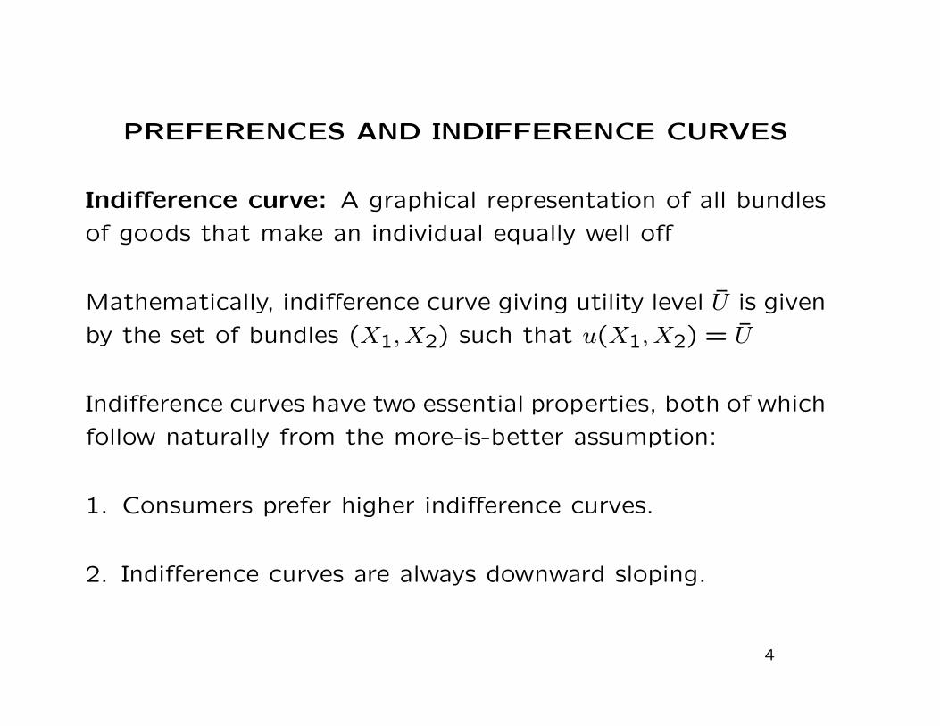
Indifference curve: A graphical representation of all bundles

of goods that make an individual equally well off

Mathematically, indifference curve giving utility level U is given

by the set of bundles (X1, X2) such that u(X1, X2) = U

Indifference curves have two essential properties, both of which

follow naturally from the more-is-better assumption:

1. Consumers prefer higher indifference curves.

2. Indifference curves are always downward sloping.

4

Public Finance and Public Policy Jonathan Gruber Fourth Edition Copyright © 2012 Worth Publishers

C H A P T E R 2 ■ T H E O R E T I C A L T O O L S O F P U B L I C F I N A N C E

6 of 46

2.1

Preferences and Indifference Curves

MARGINAL UTILITY

Marginal utility: The additional increment to utility obtainedby consuming an additional unit of a good:

Marginal utility of good 1 is defined as:

MU1 =∂u

∂X1'

u(X1 + dX1, X2)− u(X1, X2)

dX1

It is the derivative of utility with respect to X1 keeping X2constant (called the partial derivative)

Example:

u(X1, X2) =√X1 ·X2 ⇒

∂u

∂X1=

√X2

2√X1

This utility function described exhibits the important principleof diminishing marginal utility: ∂u/∂X1 decreases with X1:the consumption of each additional unit of a good gives lessextra utility than the consumption of the previous unit

6

MARGINAL RATE OF SUBSTITUTION

Marginal rate of substitution (MRS): The MRS is equal to

(minus) the slope of the indifference curve, the rate at which

the consumer will trade the good on the vertical axis for the

good on the horizontal axis.

Marginal rate of substitution between good 1 and good 2 is:

MRS1,2 =MU1

MU2

Individual is indifferent between 1 unit of good 1 and MRS1,2

units of good 2.

Example:

u(X1, X2) =√X1 ·X2 ⇒MRS1,2 =

X2

X1

7



13 of 46

Marginal Rate of Substitution

2.1

BUDGET CONSTRAINT

Budget constraint: A mathematical representation of all the

combinations of goods an individual can afford to buy if she

spends her entire income.

p1X1 + p2X2 = Y

with pi price of good i, and Y disposable income.

Budget constraint defines a linear set of bundles the consumer

can purchase with its disposable income Y

X2 =Y

p2−

p1

p2X1

The slope of the budget constraint is −p1/p2

9



15 of 46

Budget Constraints

2.1

UTILITY MAXIMIZATION

Individual maximizes utility subject to budget constraint:

maxX1,X2

u(X1, X2) subject to p1X1 + p2X2 = Y

Solution: MRS1,2 =p1

p2

Proof: Budget implies that X2 = (Y − p1X1)/p2

Individual chooses X1 to maximize u(X1, (Y − p1X1)/p2)

The first order condition (FOC) is:

∂u

∂X1−

p1

p2·∂u

∂X2= 0.

At the optimal choice, the individual is indifferent between

buying 1 extra unit of good 1 for $ p1 and buying p1/p2 extra

units of good 2 (also for $ p1).

11



18 of 46

2.1

Putting It All Together: Constrained Choice

INCOME AND SUBSTITUTION EFFECTS

Let us denote by p = (p1, p2) the price vector

Individual maximization generates demand functions X1(p, Y )

and X2(p, Y )

How does X1(p, Y ) vary with p and Y ?

Those are called price and income effects

Example: u(X1, X2) =√X1 ·X2 then MRS1,2 = X2/X1.

Utility maximization implies X2/X1 = p1/p2 and hence p1X1 = p2X2

Budget constraint p1X1 + p2X2 = Y implies p1X1 = p2X2 = Y/2

Demand functions: X1(p, Y ) = Y/(2p1) and X2(p, Y ) = Y/(2p2)

13

INCOME EFFECTS

Income effect is the effect of giving extra income Y on the

demand for goods: How does X1(p, Y ) vary with Y ?

Normal goods: Goods for which demand increases as income

Y rises: X1(p, Y ) increases with Y (most goods are normal)

Inferior goods: Goods for which demand falls as income Y

rises: X1(p, Y ) decreases with Y (example: you use public

transportation less when you are rich enough to buy a car)

Example: if leisure is a normal good, you work less (i.e. get

more leisure) if you are given a transfer

14

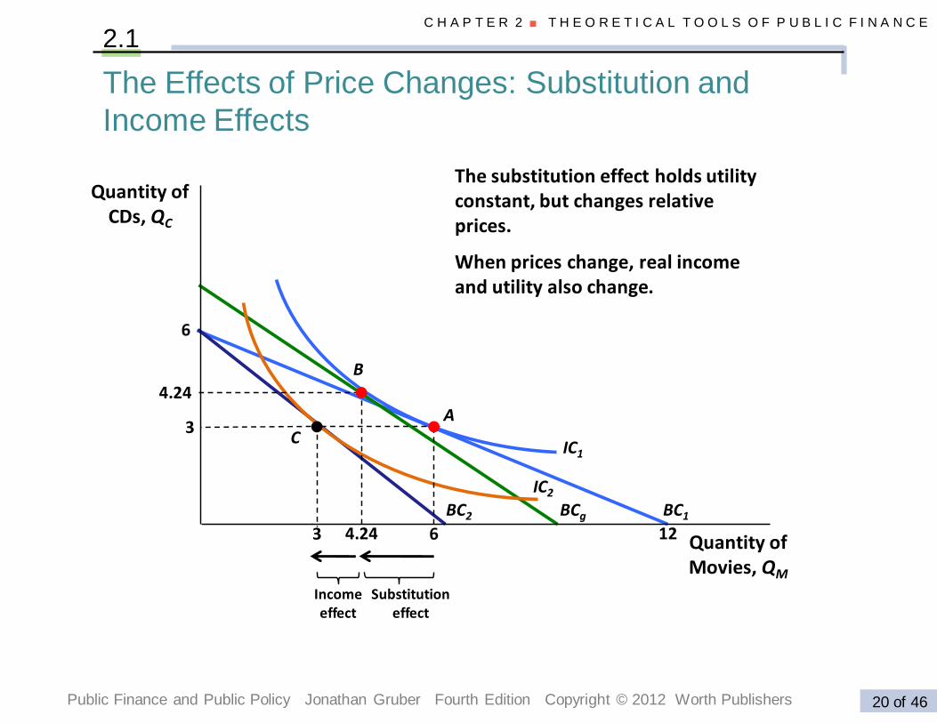
PRICE EFFECTS

How does X1(p1, p2, Y ) vary with p1?

Changing p1 affects the slope of the budget constraint and

can be decomposed into 2 effects:

1) Substitution effect: Holding utility constant, a relative

rise in the price of a good will always cause an individual to

choose less of that good

2) Income effect: A rise in the price of a good will typically

cause an individual to choose less of all goods because her

income can purchase less than before

For normal goods, an increase in p1 reduces X1(p1, p2, Y )

through both substitution and income effects

15



20 of 46

Quantity of CDs, QC

Quantity of Movies, QM

BC1BCgBC2

B

AC

6

4.24

3

3 4.24 6

IC1

IC2

Income effect

Substitution effect

The Effects of Price Changes: Substitution and

Income Effects

2.1

The substitution effect holds utility constant, but changes relative prices.

When prices change, real income and utility also change.

12



27 of 46

2.3

Demand Curves

ELASTICITY OF DEMAND

Each individual has a demand for each good that depends on

the price p of the good. Aggregating across all individuals, we

get aggregate demand D(p) for the good

At price p, demand is D(p) and p is the $ value for consumers

of the marginal (last) unit consumed

Demand graph: quantity on X-axis, price on Y-axis

Elasticity of demand ε: The % change in demand caused by

a 1% change in the price of that good:

ε =% change in quantity demanded

% change in price=

∆D/D

∆p/p=

p

D

dD

dp

Elasticities are widely used because they are unit free

18

PROPERTIES OF ELASTICITY OF DEMAND

1) Typically negative, since quantity demanded typically falls

as price rises.

2) Typically not constant along a demand curve.

3) With vertical demand curve, demand is perfectly inelastic

(ε = 0).

4) With horizontal demand curve, demand is perfectly elastic

(ε = −∞).

5) The effect of one good’s prices on the demand for another

good is the cross-price elasticity. Typically, not zero.

19

PRODUCERS

Producers (typically firms) use technology to transform inputs

(labor and capital) into outputs (consumption goods)

Goal of producers is to maximize profits = sales of outputs

minus costs of inputs

Production decisions (for given prices) define supply functions

20

SUPPLY CURVES

Marginal cost: The incremental cost to a firm of producingone more unit of a good

Profits: The difference between a firm’s revenues and costs,maximized when marginal revenues equal marginal costs

Supply curve S(p) is the quantity that firms in aggregate arewilling to supply at each price: typically upward sloping withprice due to decreasing returns to scale

At price p, producers produce S(p), and the $ cost of producingthe marginal (last) unit is p

Elasticity of supply εS is defined as

εS =% change in quantity supplied

% change in price=

∆S/S

∆p/p=

p

S

dS

dp

21

MARKET EQUILIBRIUM

Demanders and suppliers interact on markets

Market equilibrium: The equilibrium is the price p∗ such that

D(p∗) = S(p∗)

In the simple diagram, p∗ is unique if D(p) decreases with p

and S(p) increases with p

If p > p∗, then supply exceeds demand, and price needs to fall

to equilibrate supply and demand

If p < p∗, then demand exceeds supply, and price needs to

increase to equilibrate supply and demand

22



33 of 46

Equilibrium: Graphical Representation

2.3

SOCIAL EFFICIENCY

Social efficiency represents the net gains to society from alltrades that are made in a particular market, and it consists oftwo components: consumer and producer surplus.

Consumer surplus: The benefit that consumers derive fromconsuming a good, above and beyond the price they paid forthe good. It is the area below demand curve and above marketprice.

Producer surplus: The benefit producers derive from sellinga good, above and beyond the cost of producing that good.It is the area above supply curve and below market price.

Total social surplus (social efficiency): The sum of con-sumer surplus and producer surplus. It is the area above supplycurve and below demand curve.

24



35 of 46

Consumer Surplus: Graphical Representation

2.3

• Consumer surplus is the area under the demand curve since demand = willingness to pay.



36 of 46

Producer Surplus: Graphical Representation

2.3

• Producer surplus is the area above the supply curve since supply = marginal cost.



37 of 46

Social Surplus: Graphical Representation

2.3

COMPETITIVE EQUILIBRIUM MAXIMIZES

SOCIAL EFFICIENCY

First Fundamental Theorem of Welfare Economics:

The competitive equilibrium where supply equals demand, max-

imizes social efficiency.

Deadweight loss: The reduction in social efficiency from

denying trades for which benefits exceed costs when quantity

differs from the socially efficient quantity

Key rule: Deadweight loss triangles point to the social opti-

mum, and grow outward from there.

The simple efficiency result from the 1-good diagram can

be generalized into the first welfare theorem (Arrow-Debreu,

1940s), most important result in economics

28

Generalization: 1st Welfare Theorem

1st Welfare Theorem: If (1) no externalities, (2) perfectcompetition [individuals and firms are price takers], (3) per-fect information, (4) agents are rational, then private marketequilibrium is Pareto efficient

Pareto efficient: Impossible to find a technologically feasibleallocation that improves everybody’s welfare

Pareto efficiency is desirable but a very weak requirement (asingle person consuming everything is Pareto efficient)

Government intervention may be particularly desirable if theassumptions of the 1st welfare theorem fail, i.e., when thereare market failures ⇒ Govt intervention can potentially im-prove everybody’s welfare

Second part of class considers such market failure situations

29

2nd Welfare Theorem

Even with no market failures, free market outcome might gen-

erate substantial inequality. Inequality is seen as the biggest

issue with market economies.

2nd Welfare Theorem: Any Pareto Efficient allocation can

be reached by

(1) Suitable redistribution of initial endowments [individualized

lump-sum taxes based on individual characteristics and not

behavior]

(2) Then letting markets work freely

⇒ No conflict between efficiency and equity

30

2nd Welfare Theorem fallacy

In reality, 2nd welfare theorem does not work because redis-

tribution of initial endowments is not feasible (because initial

endowments cannot be observed by the government)

⇒ govt needs to use distortionary taxes and transfers based

on economic outcomes (such as income or working situation)

⇒ Conflict between efficiency and equity: Equity-Efficiency

trade-off

First part of class considers policies that trade-off equity and

efficiency

31

Illustration of 2nd Welfare Theorem Fallacy

Suppose economy is populated 50% with disabled people un-able to work (hence they earn $0) and 50% with able peoplewho can work and earn $100

Free market outcome: disabled have $0, able have $100

2nd welfare theorem: govt is able to tell apart the disabledfrom the able [even if the able do not work]

⇒ can tax the able by $50 [regardless of whether they work or not] to give$50 to each disabled person ⇒ the able keep working [otherwise they’dhave zero income and still have to pay $50]

Real world: govt can’t tell apart disabled from non workingable

⇒ $50 tax on workers + $50 transfer on non workers destroys all incentivesto work ⇒ govt can no longer do full redistribution ⇒ Trade-off betweenequity and size of the pie

32

SOCIAL WELFARE FUNCTIONS

Economists evaluate welfare using social welfare functions

Social welfare function (SWF): A function that combines

the utility functions of all individuals into an overall social

utility function.

33

UTILITARIAN SOCIAL WELFARE FUNCTION

With a utilitarian social welfare function, society’s goal is to

maximize the sum of individual utilities:

SWF = U1 + U2 + ... + UN

The utilities of all individuals are given equal weight, and

summed to get total social welfare

If marginal utility of money decreases with income (satiation),

utilitarian criterion values redistribution from rich to poor

Taking $1 for a rich person decreases his utility by a small amount, givingthe $1 to a poor person increases his utility by a large amount ⇒ Transfersfrom rich to poor increase total utility

34

RAWLSIAN SOCIAL WELFARE FUNCTION

Rawls (1971) proposed that society’s goal should be to max-

imize the well-being of its worst-off member. The Rawlsian

SWF has the form:

SWF = min(U1, U2, ..., UN)

Since social welfare is determined by the minimum utility in

society, social welfare is maximized by maximizing the well-

being of the worst-off person in society (=maxi-min)

Rawlsian criterion is even more redistributive than utilitarian

criterion: society wants to extract as much tax revenue as

possible from the middle and rich to make transfers to the

poor as large as possible

35

OTHER SOCIAL JUSTICE PRINCIPLES

Standard welfarist approach is based on individual utilities.This fails to capture important elements of actual debateson redistribution and fairness

1) Just deserts: Individuals should receive compensation con-gruent with their contributions (libertarian)

2) Commodity egalitarianism: Society should ensure thatindividuals meet a set of basic needs (seen as rights) but thatbeyond that point income distribution is irrelevant

⇒ Rich countries today consider free K-12 education, universal health care,decent retirement/disability benefits as rights

3) Equality of opportunity: Society should ensure that allindividuals have equal opportunities for success

⇒ Individuals should be compensated for inequalities they are not respon-sible for (e.g., family background, inheritance, intrinsic ability) but not forinequalities they are responsible for (being hard working vs. loving leisure)

36

TESTING PEOPLE SOCIAL PREFERENCES

Saez-Stantcheva ’16 survey people online (using Amazon MTurk)

by asking hypothetical questions to elicit social preferences.

Key findings:

1) People typically do not have “utilitarian” social justice prin-

ciples (consumption lover not seen as more deserving than

frugal person)

2) People put weight on whether income has been earned

through effort vs. not (hard working vs. leisure lover)

3) People put a lot of weight of what people would have done

absent the government intervention (deserving poor vs. free

loaders)

37

Individual A is most deserving of the $1,000 tax break

Individual B is most deserving of the $1,000 tax break

Both individuals are exactly equally deserving of the tax $1,000 break

Which of the following two individuals do you think is most deserving of a $1,000 tax break? Individual A earns $50,000 per year, pays $10,000 in taxes and hence nets out $40,000. She greatly enjoys spendingmoney, going out to expensive restaurants, or traveling to fancy destinations. She always feels that she has too littlemoney to spend. Individual B earns the same amount, $50,000 per year, also pays $10,000 in taxes and hence also nets out $40,000.However, she is a very frugal person who feels that her current income is sufficient to satisfy her needs.

>>

Source: survey in Saez and Stantcheva (2013)

Individual A is most deserving of the $1,000 tax break

Individual B is most deserving of the $1,000 tax break

Both individuals are exactly equally deserving of the $1,000 tax break

Which of the following two individuals is most deserving of a $1,000 tax break? Individual A earns $30,000 per year, by working in two different jobs, 60 hours per week at $10/hour. She pays $6,000 intaxes and nets out $24,000. She is very hardworking but she does not have highpaying jobs so that her wage is low. Individual B also earns the same amount, $30,000 per year, by working parttime for 20 hours per week at $30/hour. Shealso pays $6,000 in taxes and hence nets out $24,000. She has a good wage rate per hour, but she prefers working lessand earning less to enjoy other, nonwork activities.

>>


We assume now that the government can increase benefits by $1,000 for some recipients of government benefits.

Which of the following four individuals is most deserving of the $1,000 increase in benefits?

Please drag and drop the four individuals into the appropriate boxes on the left. The upper box, marked 1 shouldcontain the individual you think is most deserving. The box labeled "2" should contain the second mostdeserving individual, etc.. Please note that you can put two individuals in the same box if you think that they areequally deserving.

Individual A gets $15,000 per year in Disability Benefits because she cannot work due to a disability and has no otherresources.

Individual B gets $15,000 per year in Unemployment Benefits and has no other resources. She lost her job and has notbeen able to find a new job even though she has been actively looking for one.

Individual C gets $15,000 pear year in Unemployment Benefits and has no other resources. She lost her job but has notbeen looking actively for a new job, because she prefers getting less but not having to work.

Individual D gets $15,000 per year in Welfare Benefits and Food Stamps and has no other resources. She is not lookingfor a job actively because she can get by living off those government provided benefits.

Items 1 = Individual most deserving of a $1,000 benefit increase

2

3

4

Individual A

Individual B

Individual C

Individual D


(1) (2) (3) (4)A. Consumption lover vs. Frugal

Consumption lover > Frugal

Consumption lover = Frugal

Consumption lover < Frugal

# obs. = 1,125 4.1% 74.4% 21.5%

B. Hardworking vs. leisure loverHardworking > Leisure lover

Hardworking = Leisure lover

Hardworking < Leisure lover

# obs. = 1,121 42.7% 54.4% 2.9%

C. Transfer Recipients and free loaders

# obs. = 1,098Disabled person unable to work

Unemployed looking for work

Unemployed not looking for work

Welfare recipient not looking for work

Average rank (1-‐4) assigned 1.4 1.6 3.0 3.5% assigned first rank 57.5% 37.3% 2.7% 2.5%% assigned last rank 2.3% 2.9% 25.0% 70.8%

Table 2: Revealed Social Preferences

Notes: This table reports preferences for giving a tax break and or a benefit increase across individuals in variousscenarios. Panel A considers two individuals with the same earnings, same taxes, and same disposable income buthigh marginal utility of income (consumption lover) vs. low marginal utility of income (frugal). In contrast toutilitarianism, 74% of people report that consumption loving is irrelevant and 21.5% think the frugal person is mostdeserving. Panel B considers two individuals with the same earnings, same taxes, and same disposable income butdifferent wage rates and hence different work hours. 54.4% think hours of work is irrelevant and 42.7% think thehardworking low wage person is more deserving. Panel C considers transfer recipients receiving the same benefitlevels. Subjects find the disabled person unable to work and the unemployed person looking for work much moredeserving than the abled bodied unemployed or welfare recipient not looking for work.

ACTUAL SOCIAL PREFERENCES

General conclusion: People favor redistribution if they feelinequalities are “unfair” but unfair means different things todifferent people

⇒ Redistribution supported when people don’t have control[education for children, health insurance for the sick, retire-ment/disability benefits for the elderly/disabled unable to work]

⇒ Less support when people have some or full control [unem-ployment, being low income]

Conservatives tend to frame things: individuals have control(personal responsibility), govt should just enforce rules

Liberals tend to frame things: many forces in society beyondindividuals’ control (“we are all in this together”), societyshould provide nurturingSee Lakoff (1996) for how liberals and conservative think

40

Conclusion: Two General Rules for Govt Intervention

1) Market Failures: Government intervention can help if

there are market failures

2) Redistribution: Free market generates inequality. Govt

taxes and spending can reduce inequality

First part of course will analyze 2), second part of course will

analyze 1)

[we are inverting the ordering relative to Gruber’s texbook so

as to cover topics related to Professor Saez’ research first].

41

REFERENCES

Gruber, Jonathan, Public Finance and Public Policy, 2016 Worth Publish-ers, Chapter 2

Lakoff, George, 1996. Moral Politics: How Liberals and ConservativesThink, 2nd edition 2010. (web)

Rawls, John, A Theory of Justice, 1971, revised in 1999, Cambridge:Harvard University Press

Saez, Emmanuel and Stefanie Stantcheva “Generalized Social MarginalWelfare Weights for Optimal Tax Theory,” American Economic Review2016. (web)

42

https://georgelakoff.com/

http://eml.berkeley.edu/~saez/saez-stantchevaAER16.pdf

theoretical tools of public finance (chapter 2 in gruber’s...

Documents