Education

131 Undergraduate Public Economics

Emmanuel Saez

UC Berkeley

1

Education

Education is one of the largest public goods provided by gov-

ernment

Approximately 5.5% of GDP or 1/6 of government expenditure

in the US

About 80% of spending done at the state and local level

Focus of an extensive body of research in the rapidly expanding

field of economics of education

2

Why Should the Government Be Involved in Education?

Ex-ante not obvious because education does not look like a

public good

1) Returns to education are largely private

2) Education is excludable

⇒ we should expect students to invest roughly the optimal

amount in their own education

3

Why Should the Government Be Involved in Education?

Four motives for government intervention:

1) Externalities (productivity spillovers, crime, citizenship)

2) Family failures: Divergence between parent and child prefer-

ences (some parents may not take good care of their children)

3) Borrowing constraints (poor but talented students may not

be able to borrow against future earnings to get an education)

4) Individual failures: young people might not do what is in

their long-run interest due to self-control problems or lack of

information

4

1) Externalities of education on crime and voting

Crimei = α+ βEduci + εi

Observational regression comparing the educated vs. not-educated likelybiased because propensity to crime εi is negatively correlated with Educi.

Lochner and Moretti (2004) use as instrument changes in state compulsoryattendance laws: State T increases compulsory attendance from 9 to 10years at time t, State C does not.

Can look at effect on education, and then look at effect on crime usingDifference-in-difference

They show that an extra year of schooling reduces incarceration ratessignificantly

0.1 pct point decline for white males relative to a mean of 1%

0.3 pct point decline for black males relative to mean of 3%

⇒ Gap in schooling between whites and blacks accounts for more than1/4 difference in crime rates

Social return to education exceeds private return by 25% based purely onreduction in crime

Moretti, Mulligan, Oreopoulos (2003) find positive effects of education onlikelihood of voting using same strategy

5

2) Divergences between parent and child preferences

Hard to find direct evidence

Duflo (2003) shows evidence that grandmothers spend morethan grandfathers on female grandchildren

Duflo (2003) uses pension reform in 1992 in South-Africa giv-ing all Blacks (65+) a minimum pension when household in-come is low (before, only whites could get the pension underApartheid)

Duflo (2003) finds that pension availability improves the weightfor height Z-score of female grandchildren (nutrition improves)but only when a grandmother gets the pension (and not whena grandfather does)

⇒ Parents preferences matter for kids outcomes

6

Duflo 9

The identification assumption underlying this exercise is that there is no sys-tematic difference in nutrition between eligible and noneligible households withan elderly member. As I discuss later, this assumption may be problematic, andI present results for an alternative specification that relaxes it.

Results

The results from estimating equation 1 are presented in table 3. Columns 1–3do not distinguish by gender of the eligible household member. For girls thecoefficient is positive but insignificant without controlling for the presence ofnoneligible members over age 50 (column 1). When these controls are introduced,the coefficient more than doubles (0.35) and becomes significant (column 2).

Table 3. Effect of the Old-Age Pension Program on Weight for Height: olsand 2sls Regressions

ols 2sls

Variable (1) (2) (3) (4) (5) (6) (7)

GirlsEligible household 0.14 0.35* 0.34*

(0.12) (0.17) (0.17)Woman eligiblea 0.24* 0.61* 0.61* 1.19*

(0.12) (0.19) (0.19) (0.41)Man eligibleb –0.011 0.11 0.056 –0.097

(0.22) (0.28) (0.19) (0.74)Observations 1574 1574 1533 1574 1574 1533 1533

BoysEligible household 0.0012 0.022 0.030

(0.13) (0.22) (0.24)Woman eligiblea 0.066 0.28 0.31 0.58

(0.14) (0.28) (0.28) (0.53)Man eligibleb –0.059 –0.25 –0.25 –0.69

(0.22) (0.34) (0.35) (0.91)Observations 1670 1670 1627 1670 1670 1627 1627

Control variablesPresence of older membersc No Yes Yes No Yes Yes YesFamily background variablesd No No Yes No No Yes YesChild age dummy variablese Yes Yes Yes Yes Yes Yes Yes

*Significant at the 5 percent level.Note: The instruments in column 7 are woman eligible and man eligible (the first stage is in table A-1).

Standard errors (robust to correlation of residuals within households and heteroscedasticity) are inparentheses.

aIn column 7 this variable is replaced by a dummy for whether a woman receives the pension.bIn column 7 this variable is replaced by a dummy for whether a man receives the pension.cPresence of a woman over age 50, a man over age 50, a woman over age 56, a man over age 56,

and a man over age 61.dFather’s age and education; mother’s age and education; rural or metropolitan residence (urban is

the omitted category); size of household; and number of members ages 0–5, 6–14, 15–24, and 25–49.eDummy variables for whether the child was born in 1991, 1990, or 1989.Source: Author’s calculations.

Source: Duflo (2003)

3) Borrowing Constraints: effects of loans

If there are no borrowing constraints (and individuals are ra-tional), current resources should not matter for educationaldecisions: invest in education only if PDV benefits > costs

Empirical evidence shows that availability of loans do mattersuggesting that borrowing constraints are an issue

Solis (2017) studies the effects of guaranteed loans on collegeattendance in Chile

Guaranteed loan is available if test score of student (equivalentof SAT for Chile) is above threshold equal to 475.

Regression discontinuity design: does discontinuity in loanavailability translate into discontinuity in college attendance?YES

⇒ Very compelling evidence that loan availability matters

8

Figure 6: RD for College enrollment. Full sample.

0.2

.4.6

.81

Pr

(Col

lege

Enr

ollm

ent)

200 400 600 800PSU score

College Enrollment Year=2007 bw=2

0.2

.4.6

.81

Pr

(Col

lege

Enr

ollm

ent)

200 400 600 800PSU score

College Enrollment Year=2008 bw=2

0.2

.4.6

.81

Pr

(Col

lege

Enr

ollm

ent)

200 400 600 800PSU score

College Enrollment Year=2009 bw=20

.2.4

.6.8

1P

r (C

olle

ge E

nrol

lmen

t)

200 400 600 800PSU score

College Enrollment; All Years; bw=2

Note: Each dot represents average college enrollment in an interval of 2 PSU points.The dashed lines represent fitted values from a 4th order spline and 95% confidence intervals for each side.The vertical line indicates the cutoff (475).These graphs show the full sample of students fulfilling all requirements to be eligible for college loans andtaking the PSU immediately after graduating from high school.

57

Source: Solis (2013)

4) Behavioral motives (individual failures): high-school

Rational education decision should be based on comparingreturns to education (higher wage later in life) vs. costs ofeducation (tuition and time)⇒ Requires that young individualsknow the return to education

Jensen (2010) shows that simply presenting information aboutrates of return to education changes behavior

1) He uses survey data for eighth-grade boys in the DominicanRepublic

Finds that the perceived returns to secondary school are ex-tremely low, despite high measured returns

2) Then carries out randomized field experiment: Studentsat randomly selected schools given information on the highermeasured returns completed on average 0.20 more years ofschool over the next four years than those who were not.

10

EFFECT OF PROVIDING INFORMATION ABOUT

RETURNS TO COLLEGE IN DOMINICAN REPUBLIC

Source: Jensen 2010

4) Behavioral motives (individual failures): university

Hoxby-Avery ’12 shows that high-achieving US students (top2% of SAT scores) from disadvantaged backgrounds apply toweaker colleges [than other high-achieving US students]

Even though top schools offer generous financial aid to tal-ented students from disadvantaged backgrounds

Mechanism: poor talented kids in “nowhere” schools do notget good advice from family/local counselors ⇒ End up at lo-cal college (often paying more than they would at top college)

⇒ Informational failure prevents poor but talented kids to ex-ploit their potential

Hoxby-Turner ’13 does randomized experiment providing per-sonalized mailing info to talented students (relevant suggestedapplications, net-cost calculator) ⇒ Significant effect on num-ber and quality of applications

12

Figure 1

Figure 2

32

Source: Hoxby, C. M., & Avery, C. 2012

Table 1College Costs and Resources by Selectivity

Selectivity (Barron's) Out-of-Pocket Costfor a Student at the

20 Percentile ofth

Family Income(includes room and

board)

Comprehensive Cost(includes room and

board)

InstructionalExpenditure per

Student

most competitive 6,754 45,540 27,001 highly competitive plus 13,755 38,603 13,732 highly competitive 17,437 35,811 12,163 very competitive plus 15,977 31,591 9,605 very competitive 23,813 29,173 8,300 competitive plus 23,552 27,436 6,970 competitive 19,400 24,166 6,542 less competitive 26,335 21,262 5,359 some or no selection, 4-year

18,981 16,638 5,119

private 2-year 14,852 17,822 6,796 public 2-year 7,573 10,543 4,991 for-profit 2-year 18,486 21,456 3,257 Notes: The sources are colleges' net cost calculators for the out-of-pocket cost column andIPEDS for the remaining columns. The net cost data were gathered for the 2009-10 school yearby the authors, for the institutions at the very competitive and more selective levels. For theinstitutions of lower selectivity, net cost estimates are based on the institution's published net costcalculator for the year closest to 2009-10--never later than 2011-12. Net costs are then reducedto approximate 2009-10 levels using the institution's own room and board and tuition net of aidnumbers from IPEDS, for the relevant years.

Table 2College Assessment Results of High Achievers, by Family Income

Income Quartile Average SAT/ACT Percentile among HighAchievers

1st quartile (lowest income) 94.1

2nd quartile 94.3

3rd quartile 94.8

4th quartile (highest income) 95.7

Notes: A "high achiever" is student with ACT or SAT scores at or above the 90th percentile anda high school grade point average of A- or above. The source is authors' calculations based onthe combined dataset (ACT, College Board, IPEDS, and other sources) described in the text.

37

Source: Hoxby, C. M., & Avery, C. 2012

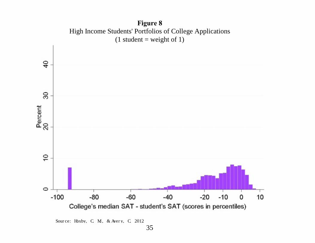
Figure 8High Income Students' Portfolios of College Applications

(1 student = weight of 1)

Figure 7Number of High Achievers per 17-year-old

darker = greater number of high achievers per 17-year-old

35Source: Hoxby, C. M., & Avery, C. 2012

Figure 10Low Income Students' Portfolios of College Applications

(1 student = weight of 1)

Figure 9Low, Middle, and High Income Students' Portfolios of College Applications

Excluding Applications to Non-Selective Institutions (1 student = weight of 1)blue = low income, brown = middle income, purple = high income

36

Source: Hoxby, C. M., & Avery, C. 2012

Two Approaches to Education Reform

A) Individual-based interventions

1) Provide vouchers for K-12 schools

2) Provide subsidies and loans to individuals for college costs

B) Improving the production process

1) Charter schools

2) Direct improvements in education production function, e.g.

teacher quality and personnel policies

3) Letting for-profit schools compete with existing public/non-

profit schools

14

PUBLIC SCHOOLS AND VOUCHERS

K-12 education is provided for free in public schools in theUS (funded by taxes)

If parents send child to private school, they have to pay privateschool tuition and do not get refunded for their taxes paidtoward public school

⇒ Strong incentives to use public schools

Educational vouchers: A fixed amount of money given bythe government to families with school-age children, who canspend it at any type of school, public or private.

A voucher effectively refunds parents for taxes paid if they donot use public schools ⇒ Puts public and private schools incompetition

15

RATIONALES FOR VOUCHERS

(1) Consumer Sovereignty: Vouchers allow families to more

closely match their educational choices with their tastes.

(2) Competition: Vouchers allow the education market to

benefit from the competitive pressures that make private mar-

kets function efficiently.

16

PROBLEMS WITH EDUCATIONAL VOUCHERS

1) Vouchers Will Lead to Segregation: Vouchers have the

potential to reintroduce segregation along many dimensions,

such as race, income, or child ability.

2) Vouchers Benefit kids from richer background: The

government would pay a portion of the private school costs

that students and their families are currently paying themselves

3) The Education Market May not Be Competitive: A

large fraction of parents do not actively search the best pos-

sible school for their kids

17

Estimating the Effects of Voucher Programs

Rouse (1998) studied the effect of the Milwaukee voucher program on theachievement of students who used their vouchers to finance a move toprivate schools

1) She noted that one cannot directly compare students who do and donot use vouchers, since they may differ along many dimensions ⇒ Thisselective use of vouchers would bias any comparison between the groups.

2) Oversubscribed schools had to select randomly from all applicants, usinga lottery (generates a quasi-experiment) ⇒ Comparing lottery winners tolosers, finds slight improvement in math scores (no difference in reading)

In the United States, about 10% of students are enrolled in private schools,a proportion that doubles or triples in the low-income developing world

Angrist et al. 2002 shows that lottery voucher program had strong positiveeffects on education in Colombia

External validity issue: voucher lottery strategy estimates effects of vouch-ers on families motivated to use them (entered the lottery). Unmotivatedparents might not be affected by vouchers.

18

Charter Schools

Some school districts have not offered vouchers for private

schools but have instead allowed students to choose freely

among public schools.

Charter schools: Schools financed with public funds that are

not usually under the direct supervision of local school boards

or subject to all state regulations for schools. Have more

flexibility to recruit teachers / adjust hours / curriculum

19

Estimating the Effects of Charter Schools

Oversubscribed charter schools also use a lottery to assign admissions

Generates randomized experiment allowing to estimate the causal effectof charter schools by comparing lottery winners and lottery losers

Angrist, Pathak, Walters AEJ’13 carry out a comprehensive analysis ofcharter schools effects in Massachusetts

Find that urban charter schools boost achievement well beyond that ofurban public school students, while non-urban charters reduce achievementfrom a higher baseline

⇒ Charter schools can have a positive or negative impact depending onwhat they do

Most effective approach to education: focus on instruction time, pupilcomportment, selective teacher hiring, and focus on traditional math andreading skills.

20

School Accountability

Making schools accountable for student performance can pro-vide incentives for schools to increase the quality of the edu-cation they offer.

Accountability programs can have two unintended effects:1) they can lead schools and teachers to “teach to the test.”2) schools can manipulate the pool of test takers and theconditions under which they take tests to maximize success.

No Child Left Behind (Key Bush administration program ineducation):

Evidence that it had small positive effects on test-scores butthis could be due primarily to “teach to the test” effects

In 2015, program turned over to the states in a more flexibleform

21

MEASURING THE RETURNS TO EDUCATION

Returns to education: The benefits that accrue to society

when students get more schooling or when they get schooling

from a higher-quality environment.

Effects of education levels on productivity

There is a large literature that shows that more education

leads to higher wages in the labor market:

Earningsi = α+ β · Educationi + εi

There is substantial controversy, however, over the implica-

tions of this correlation (β > 0).

22

Effects of Education on Earnings

1) Education as Human Capital Accumulation

human capital: A person’s stock of skills, which may beincreased by education

In that scenario, education raises earnings because it improvesproductivity

2) Education as a Screening Device

screening: A model that suggests that education providesonly a means of separating high-ability from low-ability indi-viduals and does not actually improve skills.

In that scenario, education raises individual earnings but itdoes not improve productivity (rat-race)

23

MEASURING THE RETURNS TO EDUCATION

Policy Implications

Under the human capital model, government would want tosupport education or at least provide loans to individuals sothat they can get more education and raise their productivity.

Under the screening model, however, the government wouldnot want to support more education for any given individual.

Differentiating the theories

Most of the returns to education reflect accumulation of hu-man capital rather than screening

Example: Clark-Martorell ’14 show that barely getting a high-school degree in Texas has no visible impact on later earnings

24

student’s score to be the minimum of these normalized scores. As such,students pass if and only if this normalized score is nonnegative. Thedots are cell means, and the lines are fitted values from a regression ofdiploma receipt on a fourth-order polynomial in the score ðestimatedseparately on either side of the passing cutoffÞ. The fraction of studentswith a diploma increases sharply as scores cross the passing threshold,from around 0.4 to 0.9. This implies that barely passing the last-chanceexam substantially increases the probability of earning a diploma.

A. Main Estimates

We use fuzzy regression discontinuity methods ðAngrist and Lavy 1999;Hahn et al. 2001Þ to exploit this discontinuity. In particular, we use pass-ing status on the last-chance exam as an instrumental variable for di-ploma receipt in models that control for flexible functions of the examscores ði.e., the variable on the horizontal axis in fig. 1Þ. More formally,we estimate the following equations:

Yi 5 b0 1 b1Di 1 f ðpiÞ1 εi ; ð1Þ

FIG. 1.—Last-chance exam scores and diploma receipt. The graphs are based on the last-chance sample. See table 1 and the text. Dots are test score cell means. The scores on the x -axis are the minimum of the section scores ðrecentered to be zero at the passing cutoff Þthat are taken in the last-chance exam. Lines are fourth-order polynomials fitted separatelyon either side of the passing threshold.

292 journal of political economy

This content downloaded from 169.229.128.52 on Sun, 22 Feb 2015 18:12:25 PMAll use subject to JSTOR Terms and Conditions

Source: Clark and Martorell JPE'14

tus even in the last-chance sample of students who remain in school untilthe end of grade 12. We return to this point in our discussion of the find-ings. Third, there is no indication of any jump in earnings at the passingcutoff.The estimated discontinuities reported in table 3 are consistent with

this last assertion. For each earnings outcome ði.e., for each year group-ingÞ, columns 1–4 report estimated discontinuities for first- throughfourth-order polynomials, where thepolynomials are fully interactedwithan indicator for passing the last-chance exam. For each outcome, theestimated discontinuities are small in magnitude, small relative to themean earnings of those who barely failed the exam ðcol. 1Þ and statis-tically indistinguishable from zero. Moreover, the estimates are robustto the choice of polynomial. Goodness-of-fit statistics suggest that thesecond-order polynomial is the preferred specification, and column 5reports estimates from a model that uses this preferred polynomial andcontrols for baseline covariates. In column 6 we report estimates from amodel in which the coefficients of the polynomial are restricted to be thesame on either side of the passing cutoff. These estimates are more pre-

FIG. 2.—Earnings by last-chance exam scores. The graphs are based on the last-chancesamples. See table 1 and the text. Dots are test score cell means. The scores on the x-axis arethe minimum of the section scores ðrecentered to be zero at the passing cutoff Þ that aretaken in the last-chance exam. Lines are fourth-order polynomials fitted separately oneither side of the passing threshold.

298 journal of political economy

This content downloaded from 169.229.128.52 on Sun, 22 Feb 2015 18:12:25 PMAll use subject to JSTOR Terms and Conditions

Source: Clark and Martorell JPE'14

Evidence on the Returns to Education and Screening

Basic observational approach:

Earningsi = α+ β · Educationi + εi

Amounts to comparing the earnings of people with differenteducation.

Issue: ability to earn εi might be correlated with educationchoices

Two methods try to control for this bias in estimating the truehuman capital effects of education

1) Control for underlying ability by adding variables (e.g. SAT score) inthe regression so that any remaining effect of education represents trueproductivity effects (omitted variable bias remains a concern)

2) Find exogenous variation in education (e.g., policy change induces moreeducation for some group but not for another group)

Although all of these approaches have some limitations, the result of theanalysis is surprisingly consistent: each additional year of education raiseswages by 7-10%

26

THE IMPACT OF SCHOOL QUALITY

A number of approaches have been taken to estimate the

impact of school quality on student test scores.

Two approaches have been used to address this issue: exper-

imental data, and quasi-experimental using policy changes

Findings suggest that the outcomes of efforts to improve

school quality can be very dependent on the approach taken

to improvements

27

Estimating the Effects of Class Size

Experimental example: The state of Tennessee implemented ProjectSTAR in 1985, randomly assigning 11,000 students (grades K–3) to smallclasses (13–17 students) or regular classes (22–25 students)

Krueger and Whitmore 2001 shows positive effects of small class size ontest scores

Chetty et al. 2011 linked students to college enrollment and adult earningsdata: finds small positive effects on college enrollments and adult earnings.

Note: kids and teachers also randomly assigned across classes: strongclass effects are visible (due to teachers or peers) and they have long-termeffects on college and earnings

Quasi-experimental example: By the mid-1990s, California had thelargest class sizes in the nation (29 students per class on average). TheCalifornia state government in 1996 provided strong financial incentivesfor schools to reduce their class size to 20 students per class: not mucheffects on outcomes found but controversial

28

Current Government Role in Higher Education

1. State Provision: The primary form of government fi-

nancing of higher education is direct provision of higher edu-

cation through locally and state-supported colleges and uni-

versities.

2. Pell Grants: Subsidy to higher education administered

by the federal government that provides grants to low-income

families to pay for their educational expenditures.

3. Loans: (a) direct student loans: Loans taken directly

from the Department of Education. (b) guaranteed student

loans: Loans taken from private banks for which the banks

are guaranteed repayment by the govt.

4. Tax Relief: Tax credits for higher education tuition costs

29

Public Finance and Public Policy Jonathan Gruber Third Edition Copyright © 2010 Worth Publishers 25 of 31

C H A P T E R 1 1 ■ E D U C A T I O N 11.5 The Role of the Government in Higher Education Current Government Role

What Is the Market Failure in Higher Education?

If individuals are rational, the borrowing constraint market fail-

ure can be addressed solely with government supported loans

However, if individuals are not rational (self-control problems,

myopia, lack of information), even government supported loans

might not be enough to motivate individuals to acquire higher

education

⇒ Direct tuition subsidies might be more effective

⇒ Direct help with applications

31

Effects of cash allowance on attending college in France

Fack and Grenet (2014) study the effects of aid to students

based on parental income in France

Level of aid is a discontinuous function of parental income

Regression discontinuity design: does the discontinuity in aid

translate into a discontinuity in college attendance? YES

⇒ Very compelling evidence that financial aid for higher edu-

cation matters

32

Figure 1: Income Eligibility Thresholds for the Di↵erent Levels of BCS Grant

0123456789

1011121314151617

L6 L5 L4 L3 L2 L1 L0

NotEligible

Fam

ily N

eeds

Ass

essm

ent (

FNA)

Sco

re

0 20,000 40,000 60,000 80,000 100,000Parents’ Taxable Income Two Years Before Application (Euros)

Notes: The figure shows the income eligibility thresholds for the di↵erent levels of grants (denoted L0 to L6)

awarded through the French Bourses sur criteres sociaux program in 2009. The thresholds, which depend

on the applicant’s family need assessment (FNA) score, apply to parental taxable income earned two years

before the application (x-axis). The FNA score (y-axis) is capped at 17 and has a median value of 3. Income

thresholds are expressed in 2011 euros.

Figure 2: Amount of Annual Cash Allowance Awarded to Applicants with anFNA Score of 3 Points, as Function of their Parents’ Taxable Income

L6 L5 L4 L3 L2 L1 L0(Fee Waiver)

NoGrant

01,

000

2,00

03,

000

4,00

05,

000

Amou

nt o

f Ann

ual C

ash

Allo

wan

ce (E

uros

)

0 10,000 20,000 30,000 40,000 50,000Parents’ Taxable Income Two Years Before Application (Euros)

Notes: The figure shows the amount of annual cash allowance awarded in 2009 to BCS grant applicants with a

family needs assessment (FNA) score of 3 points (median value), as a function of their parents’ taxable income

two years before the application. Applicants eligible for a level 0 grant qualify for fee waivers only. Applicants

eligible for higher levels of grant qualify for fee waivers and an annual cash allowance, the amount of which varies

with the level of grant: 1,476 euros (level 1), 2,223 euros (level 2), 2,849 euros (level 3), 3,473 euros (level 4),

3,988 euros (level 5) and 4,228 euros (level 6). Income thresholds and allowance amounts are expressed in 2011

euros.

34

Source: Fack and Grenet (2014)

Figure 5: College Enrollment Rate of Grant Applicants at Di↵erent IncomeEligibility Thresholds

(a) Fee Waiver (L0/No grant Cuto↵s)

.7.8

.91

Col

lege

Enr

ollm

ent R

ate

(Yea

r t)

−.2 −.15 −.1 −.05 0 .05 .1 .15 .2Relative Income−Distance to Eligibility Cutoff

(b) e1,500 Allowance (L1/L0 Cuto↵s)

.7.8

.91

Col

lege

Enr

ollm

ent R

ate

(Yea

r t)

−.16 −.12 −.08 −.04 0 .04 .08 .12 .16Relative Income−Distance to Eligibility Cutoff

(c) e600 Increment (L6/L5 to L2/L1 Cuto↵s)

.7.8

.91

Col

lege

Enr

ollm

ent R

ate

(Yea

r t)

−.06 −.04 −.02 0 .02 .04 .06Relative Income−Distance to Eligibility Cutoff

Notes: The circles represent the mean college enrollment rate of grant applicants per interval of relative income-

distance to the eligibility thresholds. The solid lines are the fitted values from a third-order polynomial ap-

proximation which is estimated separately on both sides of the cuto↵s. The vertical lines identify the eligibility

cuto↵s.

37

Source: Fack and Grenet (2014)

Effects of college application tutoring

Carrell-Sacerdote (2017) carry out a field experiment in NewHampshire high-schools

College students from Dartmouth help senior high-schoolersto apply to college (weekly meetings in Winter semester)

Randomization within high schools: select only 50% of seniors

Find large positive impact on women (+15 points likelihoodof enrolling in college) but small effects on men

Also find a cash bonus for applying to colleges without tutorialdoes not have any impact

⇒ Effects require time intensive tutorials (that parents/teacherstypically should be providing)

35

Role of Government in supply of Higher Education

Private non-profit universities have inelastic supply (e.g., fixedstudent bodies at top schools such as Harvard)

Historically, expansion of supply was carried out by public insti-tutions (state universities and community colleges): Example:1960 Master plan for California with 3-tier system (Commu-nity, State, UC)

Government push also central to increase attendance: GI Billafter WWII/Korea War increased college attendance by 15-20points for men born 1921-1933 (Stanley QJE’03)

Recently, states have retreated and supply has been providedby for-profit schools (get about 10% of total enrollment today)

Deming-Goldin-Katz ’12 show that for-profit schools provide little bene-fits, charge a lot, and are savvy at exploiting Fed Pell Grants and saddlestudents with debt

⇒ Symptom of market failure due to individual failures/lack of information

36

The early period of gender parity in college enrollments from 1900 to 1930(covering the birth cohorts of 1880 to 1910) was not the result of a situation whereonly an elite class sent children of both genders to college. Just 5 percent of thewomen enrolled in privately-controlled colleges in 1925 attended the elite “seven-sister” schools and only 22 percent were in any all-women’s college. Half of allAmerican college students in 1925 were in publicly-controlled institutions of highereducation, and 55 percent of women were. A substantial fraction of women duringthis period attended teacher-training colleges, and many of these schools hadtwo-year programs. In 1925, for example, 30 percent of the female enrollments

Figure 1College Graduation Rates (by 35 years) for Men and Women: Cohorts Born from1876 to 1975

1870 1880 1890 1900 1910 1920

Birth year

Frac

tion

gra

duat

ed

1930 1940 1950 1960 1970 19800.0

0.1

0.2

0.3

0.4

Females

Males

Sources: 1940 to 2000 Census of Population Integrated Public Use Micro-data Samples (IPUMS).Notes: The figure plots separately by sex the fraction of each birth cohort who had completed at least fouryears of college by age 35 for the U.S. born. When the IPUMS data allows us to look directly atthirty-five-year-olds in a given year, we use that data. Since educational attainment data was first collectedin the U.S. population censuses in 1940, we need to infer completed schooling at age 35 for cohorts bornprior to 1905 based on their educational attainment at older ages. We also don’t observe all post-1905birth cohorts at exactly age 35. We use a regression approach to adjust observed college graduation ratesfor age based on the typical proportional life-cycle evolution of educational attainment of a cohort. Theage-adjustment regressions are run on birth-cohort year cells pooled across the 1940 to 2000 IPUMS withthe log of the college graduation rate as the dependent variable and a full set of birth cohort dummiesand a quartic in age as the covariates. The details of the age-adjustment method are the same as usedby DeLong, Goldin, and Katz (2003, Figure 2–1). College graduates are those with 16 or morecompleted years of schooling for the 1940 to 1980 samples and those with a bachelor’s degree or higherin the 1990 to 2000 samples. The underlying sample includes all U.S. born residents aged 25 to 64 years.

Claudia Goldin, Lawrence F. Katz, and Ilyana Kuziemko 135

Role of Higher Education in Intergenerational Mobilily

Chetty et al. ’17 compile college level statistics on parentalincome and student earnings outcomes. Data online at (web)

Four key findings:

1) Access: Huge variation in access across schools: Ivy leaguehas more kids from top 1% families than from bottom 50%

2) Outcomes: Within good colleges, outcomes of poor vs.rich kids are similar ⇒ college is the ticket to opportunity

3) Mobility rates: Large discrepancies across colleges in frac-tion of students who come from bottom 20% and reach top20% (=mobility rate)

4) Trends: fraction poor kids stagnated in top schools (inspite of more financial aid) and dropped at best public schoolsand community colleges

38

Visit www.equality-of-opportunity.org for the full paper, college-level data, and more

The Equality of Opportunity Project

0%20

%40

%60

%80

%P

erce

nt o

f Stu

dent

s

1 2 3 4 5Parent Income Quintile

SUNY-Stony BrookColumbia

Top 1%13.7%

Top 1%0.4%

Access: Pct. of Students from each fifth of the Parent Income Distribution

Success Rates: Pct. of Students with Earnings in Top Fifth

Mobility Report Cards: The Role of Colleges in Intergenerational Mobility

Raj Chetty, John N. Friedman, Emmanuel Saez, Nicholas Turner, and Danny Yagan

Which colleges in America contribute the most to helping children climb the income ladder? How can we increase access to such colleges for children from low income families? We take a step toward answering these questions by constructing publicly available mobility report cards – statistics on students’ earnings in their early thirties and their parents’ incomes – for each college. We estimate these statistics using de-identified data from the federal government covering all students from 1999-2013, building on the Dept. of Education’s College Scorecard.

Mobility Report Cards for Columbia and SUNY-Stony Brook

Using these mobility report cards, we document four results. 1. Access. Access to colleges varies substantially across the income distribution, for example as shown between Columbia and SUNY-Stony Brook in the figure above. At “Ivy-Plus” colleges (Ivy League colleges, U. Chicago, Stanford, MIT, and Duke), more students come from families in the top 1% of the income distribution than the bottom half of the income distribution. Despite the generous financial aid offered by these institutions, students from the lowest-income families are particularly under-represented, even relative to middle-income students. Children with parents in the top 1% are 77 times more likely to attend an Ivy-Plus college than children with parents in the bottom 20%. More broadly, looking across all colleges, the degree of income segregation is comparable to income segregation across neighborhoods in the average American city. These findings challenge the perception that colleges foster interaction between children from diverse socioeconomic backgrounds.

Note: Bars show estimates of the fraction of parents in each quintile of the income distribution. Lines show estimates of the fraction of students from each of those quintiles who reach the top quintile as adults.

Mobility Report Cards: Executive Summary

Visit www.equality-of-opportunity.org for the full paper, college-level data, and more

2. Outcomes. At any given college, students from low- and high- income families have very similar earnings outcomes. For example, about 60% of students at Columbia reach the top fifth from both low and high income families. In this sense, colleges successfully “level the playing field” across enrolled students with different socioeconomic backgrounds. This finding suggests that students from low-income families who are admitted to selective colleges are not over-placed, since they do nearly as well as students from more affluent families. This result also suggests that colleges do not bear large costs in terms of student outcomes for any affirmative action that they grant students from low-income families in the admissions process. 3. Mobility Rates. We characterize differences in rates of upward mobility between colleges by defining a college’s upward mobility rate as the fraction of its students who come from a family in the bottom fifth of the income distribution and end up in the top fifth. Each college’s mobility rate is the product of access, the fraction of its students who come from families in the bottom fifth, and its success rate, the fraction of such students who reach the top fifth. Mobility rates vary substantially across colleges because there are large differences in access across colleges with similar success rates. Ivy-Plus colleges have the highest success rates, with almost 60% of students from the bottom fifth reaching the top fifth. But certain less selective universities have comparable success rates while offering much higher levels of access to low-income families. For example, 51% of students from the bottom fifth reach the top fifth at SUNY–Stony Brook. Because 16% of students at Stony Brook are from the bottom fifth compared with 4% at the Ivy-Plus colleges, Stony Brook has a bottom-to-top-fifth mobility rate of 8.4%, substantially higher than the 2.2% rate on average at Ivy-Plus colleges. The colleges that have the highest upward mobility rates, listed in the table below, are typically mid-tier public schools that have many low-income students and very good outcomes.

Top 10 Colleges by Mobility Rate (from Bottom to Top Quintile)

Note: Table lists highest-mobility-rate colleges with more than 300 students per cohort.

Rank Name Mobility Rate = Access x Success Rate

1 Cal State University – LA 9.9% 33.1% 29.9%

2 Pace University – New York 8.4% 15.2% 55.6%

3 SUNY – Stony Brook 8.4% 16.4% 51.2%

4 Technical Career Institutes 8.0% 40.3% 19.8%

5 University of Texas – Pan American 7.6% 38.7% 19.8%

6 City Univ. of New York System 7.2% 28.7% 25.2%

7 Glendale Community College 7.1% 32.4% 21.9%

8 South Texas College 6.9% 52.4% 13.2%

9 Cal State Polytechnic – Pomona 6.8% 14.9% 45.8%

10 University of Texas – El Paso 6.8% 28.0% 24.4%

Mobility Report Cards: Executive Summary

Visit www.equality-of-opportunity.org for the full paper, college-level data, and more

The differences in mobility rates across colleges are not driven by differences in the distribution of college majors or other institutional characteristics. The estimates are similar when we measure children’s income at the household instead of individual level or adjust for differences in local costs of living. If we measure “success” in earnings as reaching the top 1% of the income distribution instead of the top 20%, we find very different patterns. The colleges that channel the most children from low- or middle-income families to the top 1% are almost exclusively highly selective institutions, such as UC–Berkeley and the Ivy-Plus colleges, where 13% of students from the bottom fifth reach the top 1%. No college in the U.S. currently offers a high rate of upper-tail (top 1%) success while providing very high levels of access to low-income students. 4. Trends. Finally, we examine how access and mobility rates have changed since 2000, when our data begin. Despite substantial tuition reductions and other outreach policies, the fraction of students from low-income families at the Ivy-Plus colleges increased very little across a range of income percentiles (e.g., below the 20th, 40th, or 60th percentile). This is illustrated by the trend in the fraction of students from the bottom quintile at Harvard in the figure below. This result does not imply that the increases in financial aid had no effect on access; absent these changes, the fraction of low-income students might have fallen, especially given that real incomes of low-income families fell due to widening inequality during the 2000s.

Trends in Low-Income Access from 2000-2011 at Selected Colleges

The increase in our percentile-based measures of access at elite private colleges is smaller than suggested by the increase in the fraction of students receiving federal Pell grants – a widely-used proxy for low-income access – because the Pell eligibility threshold rose in the 2000s and the real income. Meanwhile, access at institutions with the highest mobility rates (e.g., SUNY-Stony Brook and Glendale Community College in the figure above) fell sharply over the 2000s, perhaps because

0%10

%20

%30

%40

%P

erce

nt o

f Par

ents

in th

e B

otto

m Q

uint

ile

2000 2002 2004 2006 2008 2010Year when Child was 20

Glendale Community College

SUNY-Stony Brook

UC-Berkeley

Harvard

REFERENCES

Jonathan Gruber, Public Finance and Public Policy, Fourth Edition, 2016Worth Publishers, Chapter 11

Angrist, Joshua, et al. “Vouchers for Private Schooling in Colombia: Ev-idence from a Randomized Natural Experiment.” American EconomicReview 92(5), (2002), 1535–1558.(web)

Angrist, Joshua, Parag A. Pathak, and Christopher R. Walters.“ExplainingCharter School Effectiveness.” American Economic Journal: Applied Eco-nomics, 5.4 (2013): 1-27.(web)

Carrell, Scott E., and Bruce Sacerdote. “Why Do College Going Inter-ventions Work?” No. w19031. National Bureau of Economic Research,2013. forthcoming American Economic Journal: Applied (web)

Chetty, Raj, John N. Friedman, Nathaniel Hilger, Emmanuel Saez, DianeWhitmore Schanzenbach, and Danny Yagan. “How does your kindergartenclassroom affect your earnings? Evidence from Project STAR.” QuarterlyJournal of Economics 126, no. 4 (2011): 1593-1660.(web)

Chetty, Raj, John Friedman, Emmanuel Saez, Nicholas Turner, DannyYagan. “Mobility Report Cards: The Role of Colleges in IntergenerationalMobility” Working paper 2017.(web)

40

Clark, Damon and Paco Martorell “The Signaling Value of a High SchoolDiploma” Journal of Political Economy 122(2), 282-318. (web)

Deming, David, Claudia Goldin, and Lawrence F. Katz. “The For-ProfitPostsecondary School Sector: Nimble Critters or Agile Predators?” Jour-nal of Economic Perspectives (2012), vol. 26(1), pages 139-64. (web)

Duflo, Esther, “Grandmothers and Granddaughters: Old?Age Pensionsand Intrahousehold Allocation in South Africa” World Bank Economic Re-view, 17(1) (2003): 1–25.(web)

Dynarski, Susan M. “Does Aid Matter? Measuring the Effect of StudentAid on College Attendance and Completion.” American Economic Review93.1 (2003): 279-288.(web)

Fack, Gabrielle, and Julien Grenet, “Improving College Access and Suc-cess for Low-Income Students: Evidence from a Large French Need-basedGrant Program,” American Economic Journal: Applied Economics, 2014.(web)

Goldin, Claudia, Lawrence Katz, Ilyana Kuziemko “The Homecoming ofAmerican College Women: The Reversal of the College Gender Gap”,Journal of Economic Perspectives, 2006. (web)

Hoxby, Caroline, and Christopher Avery. “The Missing“One-Offs”: TheHidden Supply of High-Achieving, Low Income Students.” No. w18586.National Bureau of Economic Research, 2012.(web)

Hoxby, Caroline, and Sarah Turner. “Expanding College Opportunitiesfor High-Achieving, Low Income Students.” SIEPR Discussion Paper No.12-014 (2013).(web)

Jensen, Robert. “The (perceived) returns to education and the demandfor schooling.” The Quarterly Journal of Economics 125.2 (2010): 515-548.(web)

Krueger, Alan B., and Diane M. Whitmore. “The effect of attending asmall class in the early grades on college-test taking and middle schooltest results: Evidence from Project STAR.” Economic Journal 111.468(2001): 1-28.web

Lochner, Lance, and Enrico Moretti. “The Effect of Education on Crime:Evidence from Prison Inmates, Arrests, and Self-Reports.” American Eco-nomic Review 94.1 (2004): 155-189.(web)

Milligan, Kevin, Enrico Moretti, and Philip Oreopoulos. “Does educationimprove citizenship? Evidence from the United States and the UnitedKingdom.” Journal of Public Economics 88.9 (2004): 1667-1695.(web)

Rouse, Cecilia Elena. “Private school vouchers and student achievement:An evaluation of the Milwaukee parental choice program.” Quarterly Jour-nal of Economics 113.2 (1998): 553-602.(web)

Solis, Alex “Credit Access and College Enrollment”, Journal of PoliticalEconomy 125(2), 2017: 562-622. (web)

Stanley, Marcus. “College education and the midcentury GI Bills.” Quar-terly Journal of Economics 118.2 (2003): 671-708.(web)