thermal conductivity of soils from the analysis of boring logs
TRANSCRIPT
8/16/2019 Thermal Conductivity of Soils From the Analysis of Boring Logs
http://slidepdf.com/reader/full/thermal-conductivity-of-soils-from-the-analysis-of-boring-logs 1/96
University of South FloridaScholar Commons
G a a ! ! ! a D% ! a %* G a a ! Sc$**'
10-21-2010
Termal Conductivity of Soils from the Analysis Boring LogsNicole M. Pauly University of South Florida
F*''* $% a a % %* a' * & a :$5+:// c$*'a c* * . .! /!Pa * $! A ! %ca S %! C* *
% ! % % b * #$ * * * !! a *+! acc! b $! G a a ! Sc$**' a Sc$*'a C* * . I $a b!! acc!+ ! * % c' %* % G a a !! ! a D% ! a %* b a a $* % ! a % % a * * Sc$*'a C* * . F* * ! % * a %* , +'!a ! c* ac c$*'a c* * @ .! .
Sc$*'a C* * C% a %*Pa ' , N%c*'! M., " ! a' C* c % % * S*%' * $! A a' % * B* % # L*# " (2010).Graduate Teses and Dissertations.$5+:// c$*'a c* * . .! /! /3614
8/16/2019 Thermal Conductivity of Soils From the Analysis of Boring Logs
http://slidepdf.com/reader/full/thermal-conductivity-of-soils-from-the-analysis-of-boring-logs 2/96
Thermal Conductivity of Soils from the Analysis of Boring Logs
by
Nicole M. Pauly
A thesis submitted in partial fulfillmentof the requirements for the degree of
Master of Science in Civil EngineeringDepartment of Civil and Environmental Engineering
College of EngineeringUniversity of South Florida
Major Professor: A. Gray Mullins, Ph.D.Rajan Sen, Ph.D.
Mike Stokes, Ph.D.
Date of Approval:October 21, 2010
Keywords: Thermal Conductivity, Diffusivity, Integrity Testing, Drilled Shaft,Standard Penetration Test
Copyright © 2010, Nicole M. Pauly
8/16/2019 Thermal Conductivity of Soils From the Analysis of Boring Logs
http://slidepdf.com/reader/full/thermal-conductivity-of-soils-from-the-analysis-of-boring-logs 3/96
i
Table of Contents
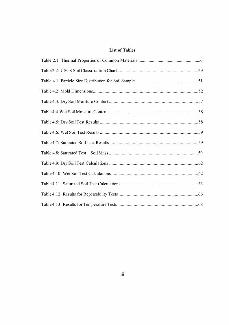
List of Tables................................................................................................................. iii
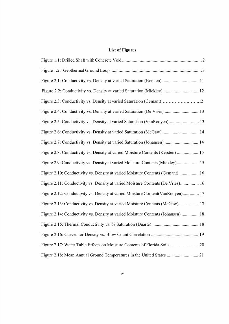
List of Figures ............................................................................................................... iv
List of Symbols and Abbreviations .............................................................................. viii
Abstract ......................................................................................................................... ix
Chapter 1 - Introduction ...................................................................................................1
1.1 Organization of Thesis ...................................................................................4
Chapter 2 - Literature Review ..........................................................................................6
2.1 Overview .......................................................................................................6
2.2 Thermal Conductivity of Soils (Background) .................................................8
2.3 Properties and Measurement Correlations ..................................................... 19
2.3.1 Boring Log Measurements ............................................................. 19
2.3.2 Density .......................................................................................... 19
2.3.3 Moisture Content ........................................................................... 20
2.3.4 Temperature................................................................................... 20
2.4 Standard Soil Testing Methods ..................................................................... 21
2.4.1 Standard Penetration Test .............................................................. 22
2.4.2 Thermal Conductivity Testing ........................................................ 23
2.4.3 Relative Density Test ..................................................................... 26
2.4.4 Soil Classification .......................................................................... 28
8/16/2019 Thermal Conductivity of Soils From the Analysis of Boring Logs
http://slidepdf.com/reader/full/thermal-conductivity-of-soils-from-the-analysis-of-boring-logs 4/96
ii
2.4.5 Thermal Integrity Profiling ............................................................ 29
Chapter 3 - Algorithm Development .............................................................................. 31
3.1 Command Buttons ........................................................................................ 33
3.2 Soil Classification ........................................................................................ 33
3.3 Moisture Content .......................................................................................... 34
3.4 Density ......................................................................................................... 37
3.5 Thermal Conductivity................................................................................... 38
3.6 Plotting ........................................................................................................ 46
Chapter 4 - Testing and Evaluation ................................................................................ 48
4.1 Equipment .................................................................................................... 48
4.2 Laboratory Testing and Evaluation ............................................................... 50
4.2.1 Soil Classification .......................................................................... 50
4.2.2 Density Variation Testing .............................................................. 51
4.2.3 Results of Density Variation Tests ................................................. 57
4.2.4 Repeatability and Temperature Tests ............................................. 65
4.2.5 Repeatability and Temperature Test Results ................................... 66
4.3 Evaluation of Theoretical Algorithms ........................................................... 69
4.3.1 Heat Capacity ................................................................................ 74
Chapter 5 - Conclusion .................................................................................................. 75
5.1 Thermal Integrity Profiling ........................................................................... 75
5.2 Future Studies .............................................................................................. 83
5.3 Summary ...................................................................................................... 83
List of References .......................................................................................................... 84
8/16/2019 Thermal Conductivity of Soils From the Analysis of Boring Logs
http://slidepdf.com/reader/full/thermal-conductivity-of-soils-from-the-analysis-of-boring-logs 5/96
iii
List of Tables
Table 2.1: Thermal Properties of Common Materials .......................................................6
Table 2.2: USCS Soil Classification Chart ..................................................................... 29
Table 4.1: Particle Size Distribution for Soil Sample ................................ ..................... 51
Table 4.2: Mold Dimensions .......................................................................................... 52
Table 4.3: Dry Soil Moisture Content ............................................................................ 57
Table 4.4 Wet Soil Moisture Content ............................................................................. 58
Table 4.5: Dry Soil Test Results .................................................................................... 58
Table 4.6: Wet Soil Test Results .................................................................................... 59
Table 4.7: Saturated Soil Test Results ............................................................................ 59
Table 4.8: Saturated Test – Soil Mass ............................................................................ 59
Table 4.9: Dry Soil Test Calculations ............................................................................ 62
Table 4.10: Wet Soil Test Calculations .......................................................................... 62
Table 4.11: Saturated Soil Test Calculations .................................................................. 63
Table 4.12: Results for Repeatability Tests .................................................................... 66
Table 4.13: Results for Temperature Tests ..................................................................... 68
8/16/2019 Thermal Conductivity of Soils From the Analysis of Boring Logs
http://slidepdf.com/reader/full/thermal-conductivity-of-soils-from-the-analysis-of-boring-logs 6/96
iv
List of Figures
Figure 1.1: Drilled Shaft with Concrete Void .................................................................... 2
Figure 1.2: Geothermal Ground Loop .............................................................................. 3
Figure 2.1: Conductivity vs. Density at varied Saturation (Kersten) ................................ 11
Figure 2.2: Conductivity vs. Density at varied Saturation (Mickley)................................ 12
Figure 2.3: Conductivity vs. Density at varied Saturation (Gemant)……………………..1 2
Figure 2.4: Conductivity vs. Density at varied Saturation (De Vries) .............................. 13
Figure 2.5: Conductivity vs. Density at varied Saturation (VanRooyen) .......................... 13
Figure 2.6: Conductivity vs. Density at varied Saturation (McGaw) ................................ 14
Figure 2.7: Conductivity vs. Density at varied Saturation (Johansen) .............................. 14
Figure 2.8: Conductivity vs. Density at varied Moisture Contents (Kersten) ................... 15
Figure 2.9: Conductivity vs. Density at varied Moisture Contents (Mickley) ................... 15
Figure 2.10: Conductivity vs. Density at varied Moisture Contents (Gemant) ................. 16
Figure 2.11: Conductivity vs. Density at varied Moisture Contents (De Vries) ................ 16
Figure 2.12: Conductivity vs. Density at varied Moisture Content(VanRooyen) .............. 17
Figure 2.13: Conductivity vs. Density at varied Moisture Contents (McGaw) ................. 17
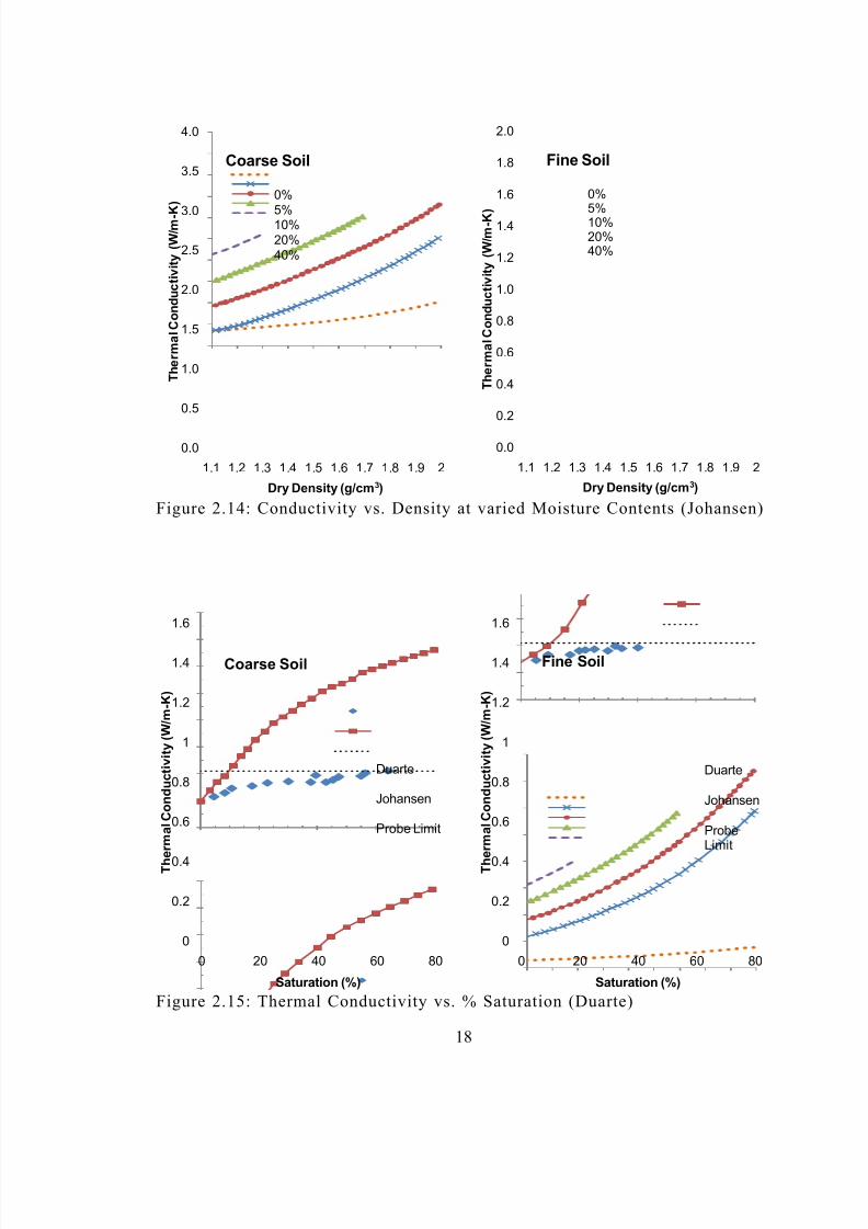
Figure 2.14: Conductivity vs. Density at varied Moisture Contents (Johansen) ............... 18
Figure 2.15: Thermal Conductivity vs. % Saturation (Duarte) ......................................... 18
Figure 2.16: Curves for Density vs. Blow Count Correlation .......................................... 19
Figure 2.17: Water Table Effects on Moisture Contents of Florida Soils ......................... 20
Figure 2.18: Mean Annual Ground Temperatures in the United States ............................ 21
8/16/2019 Thermal Conductivity of Soils From the Analysis of Boring Logs
http://slidepdf.com/reader/full/thermal-conductivity-of-soils-from-the-analysis-of-boring-logs 7/96
v
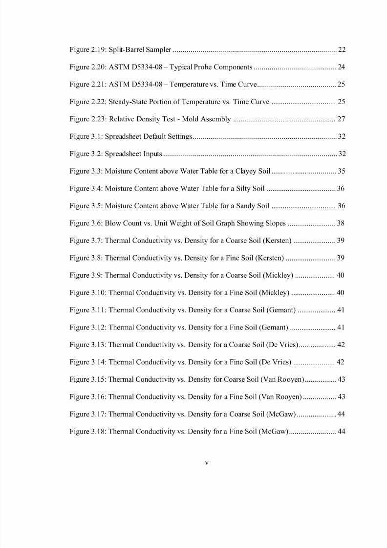
Figure 2.19: Split-Barrel Sampler ................................................................................... 22
Figure 2.20: ASTM D5334-08 – Typical Probe Components .......................................... 24
Figure 2.21: ASTM D5334-08 – Temperature vs. Time Curve ........................................ 25
Figure 2.22: Steady-State Portion of Temperature vs. Time Curve .................................. 25
Figure 2.23: Relative Density Test - Mold Assembly ...................................................... 27
Figure 3.1: Spreadsheet Default Settings ......................................................................... 32
Figure 3.2: Spreadsheet Inputs ........................................................................................ 32
Figure 3.3: Moisture Content above Water Table for a Clayey Soil ................................. 35
Figure 3.4: Moisture Content above Water Table for a Silty Soil .................................... 36
Figure 3.5: Moisture Content above Water Table for a Sandy Soil .................................. 36
Figure 3.6: Blow Count vs. Unit Weight of Soil Graph Showing Slopes ......................... 38
Figure 3.7: Thermal Conductivity vs. Density for a Coarse Soil (Kersten) ...................... 39
Figure 3.8: Thermal Conductivity vs. Density for a Fine Soil (Kersten) .......................... 39
Figure 3.9: Thermal Conductivity vs. Density for a Coarse Soil (Mickley) ..................... 40
Figure 3.10: Thermal Conductivity vs. Density for a Fine Soil (Mickley) ....................... 40
Figure 3.11: Thermal Conductivity vs. Density for a Coarse Soil (Gemant) .................... 41
Figure 3.12: Thermal Conductivity vs. Density for a Fine Soil (Gemant) ........................ 41
Figure 3.13: Thermal Conductivity vs. Density for a Coarse Soil (De Vries) ................... 42
Figure 3.14: Thermal Conductivity vs. Density for a Fine Soil (De Vries) ...................... 42
Figure 3.15: Thermal Conductivity vs. Density for Coarse Soil (Van Rooyen) ................ 43
Figure 3.16: Thermal Conductivity vs. Density for a Fine Soil (Van Rooyen) ................. 43
Figure 3.17: Thermal Conductivity vs. Density for a Coarse Soil (McGaw) .................... 44
Figure 3.18: Thermal Conductivity vs. Density for a Fine Soil (McGaw) ........................ 44
8/16/2019 Thermal Conductivity of Soils From the Analysis of Boring Logs
http://slidepdf.com/reader/full/thermal-conductivity-of-soils-from-the-analysis-of-boring-logs 8/96
vi
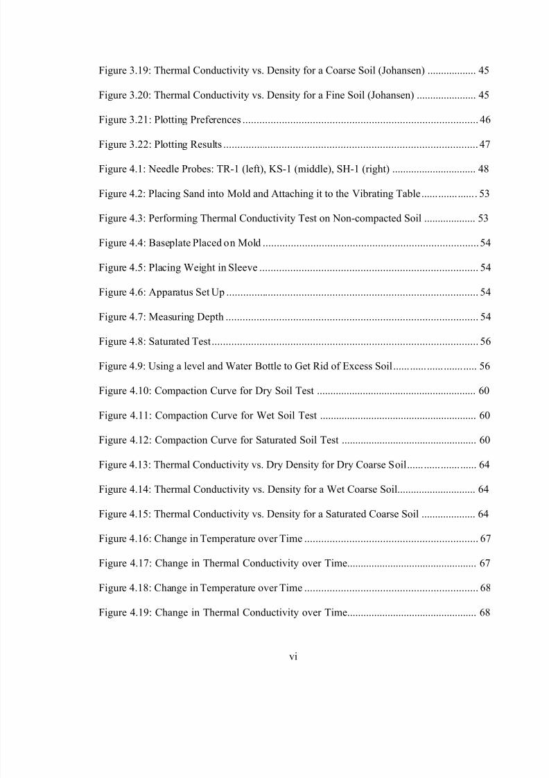
Figure 3.19: Thermal Conductivity vs. Density for a Coarse Soil (Johansen) .................. 45
Figure 3.20: Thermal Conductivity vs. Density for a Fine Soil (Johansen) ...................... 45
Figure 3.21: Plotting Preferences .................................................................................... 46
Figure 3.22: Plotting Results ........................................................................................... 47
Figure 4.1: Needle Probes: TR-1 (left), KS-1 (middle), SH-1 (right) ............................... 48
Figure 4.2: Placing Sand into Mold and Attaching it to the Vibrating Table .................... 53
Figure 4.3: Performing Thermal Conductivity Test on Non-compacted Soil ................... 53
Figure 4.4: Baseplate Placed on Mold ............................................................................. 54
Figure 4.5: Placing Weight in Sleeve .............................................................................. 54
Figure 4.6: Apparatus Set Up .......................................................................................... 54
Figure 4.7: Measuring Depth .......................................................................................... 54
Figure 4.8: Saturated Test ............................................................................................... 56
Figure 4.9: Using a level and Water Bottle to Get Rid of Excess Soil .............................. 56
Figure 4.10: Compaction Curve for Dry Soil Test ........................................................... 60
Figure 4.11: Compaction Curve for Wet Soil Test .......................................................... 60
Figure 4.12: Compaction Curve for Saturated Soil Test .................................................. 60
Figure 4.13: Thermal Conductivity vs. Dry Density for Dry Coarse Soil ......................... 64
Figure 4.14: Thermal Conductivity vs. Density for a Wet Coarse Soil............................. 64
Figure 4.15: Thermal Conductivity vs. Density for a Saturated Coarse Soil .................... 64
Figure 4.16: Change in Temperature over Time .............................................................. 67
Figure 4.17: Change in Thermal Conductivity over Time................................................ 67
Figure 4.18: Change in Temperature over Time .............................................................. 68
Figure 4.19: Change in Thermal Conductivity over Time................................................ 68
8/16/2019 Thermal Conductivity of Soils From the Analysis of Boring Logs
http://slidepdf.com/reader/full/thermal-conductivity-of-soils-from-the-analysis-of-boring-logs 9/96
vii
Figure 4.20: Boring Log for Boring BA-36 ..................................................................... 69
Figure 4.21: Inputting Project Information ...................................................................... 70
Figure 4.22: Inputting Elevations .................................................................................... 70
Figure 4.23: Inputting Depth ........................................................................................... 71
Figure 4.24: Inputting Blow Count ................................................................................. 71
Figure 4.25: Inputting Soil Type ..................................................................................... 71
Figure 4.26 – Inputted Boring Log .................................................................................. 72
Figure 4.27: Results from Clicking the Calculate Button ................................................. 73
Figure 4.28: Clicking Update after Selecting Desired Plotting Methods .......................... 73
Figure 4.29: Plot of Selected Methods and Plot of Boring Log ........................................ 73
Figure 5.1: TIP Analysis – Shaft 14-1 ............................................................................. 76
Figure 5.2: TIP Analysis – Shaft 14-2 ............................................................................. 77
Figure 5.3: TIP Analysis – Shaft 14-3 ............................................................................. 78
Figure 5.4: Thermal Conductivity and Heat Capacity for Shaft 14-1 ............................... 79
Figure 5.5: Diffusivity and Temperature Profile for Shaft 14-1 ....................................... 79
Figure 5.6: Thermal Conductivity and Heat Capacity for Shaft 14-2 ............................... 80
Figure 5.7: Diffusivity and Temperature for Shaft 14-2................................................... 80
Figure 5.8: Thermal Conductivity and Heat Capacity for Shaft 14-3 ............................... 81
Figure 5.9: Diffusivity and Temperature Profile for Shaft 14-3 ....................................... 82
Figure 5.10: Modified Diffusivity and Temperature Profile for Shaft 14-3 ...................... 82
8/16/2019 Thermal Conductivity of Soils From the Analysis of Boring Logs
http://slidepdf.com/reader/full/thermal-conductivity-of-soils-from-the-analysis-of-boring-logs 10/96
viii
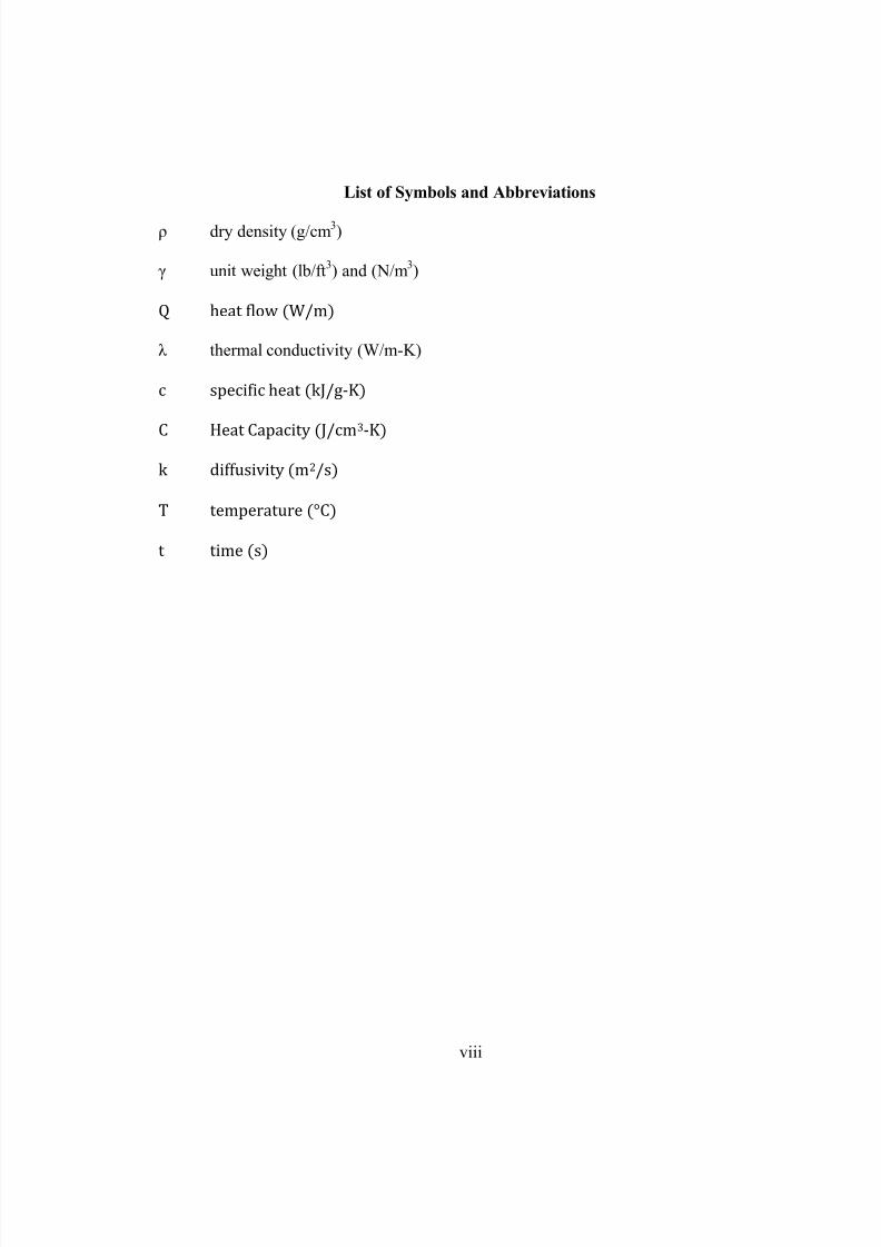
List of Symbols and Abbreviations
ρ dry density (g/cm 3)
γ unit weight (lb/ft 3) and (N/m 3)
Q heat flow (W/m)
λ thermal conductivity (W/m-K)
c specific heat (kJ/g-K)
C Heat Capacity (J/cm3
-K)
k diffusivity (m 2/s)
T temperature (°C)
t time (s)
8/16/2019 Thermal Conductivity of Soils From the Analysis of Boring Logs
http://slidepdf.com/reader/full/thermal-conductivity-of-soils-from-the-analysis-of-boring-logs 11/96
ix
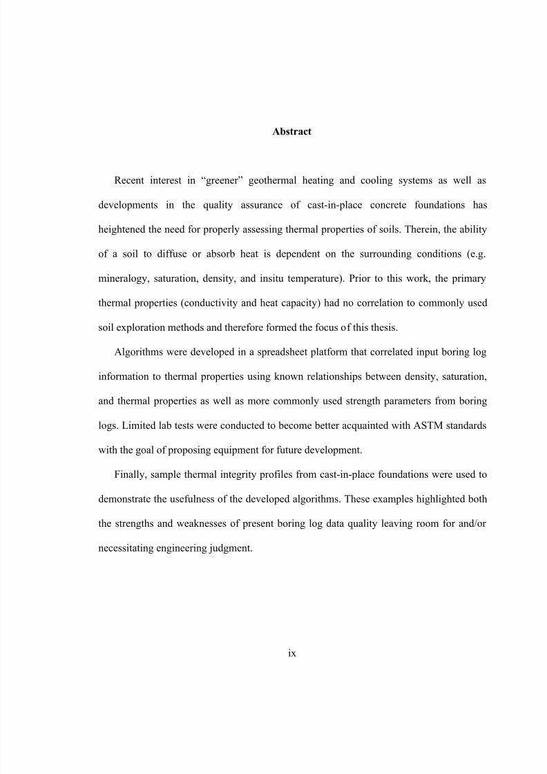
Abstract
Recent interest in “greener” geothermal heating and cooling systems as well as
developments in the quality assurance of cast-in-place concrete foundations has
heightened the need for properly assessing thermal properties of soils. Therein, the ability
of a soil to diffuse or absorb heat is dependent on the surrounding conditions (e.g.
mineralogy, saturation, density, and insitu temperature). Prior to this work, the primary
thermal properties (conductivity and heat capacity) had no correlation to commonly used
soil exploration methods and therefore formed the focus of this thesis.
Algorithms were developed in a spreadsheet platform that correlated input boring log
information to thermal properties using known relationships between density, saturation,
and thermal properties as well as more commonly used strength parameters from boring
logs. Limited lab tests were conducted to become better acquainted with ASTM standards
with the goal of proposing equipment for future development.
Finally, sample thermal integrity profiles from cast-in-place foundations were used to
demonstrate the usefulness of the developed algorithms. These examples highlighted both
the strengths and weaknesses of present boring log data quality leaving room for and/or
necessitating engineering judgment.
8/16/2019 Thermal Conductivity of Soils From the Analysis of Boring Logs
http://slidepdf.com/reader/full/thermal-conductivity-of-soils-from-the-analysis-of-boring-logs 12/96
1
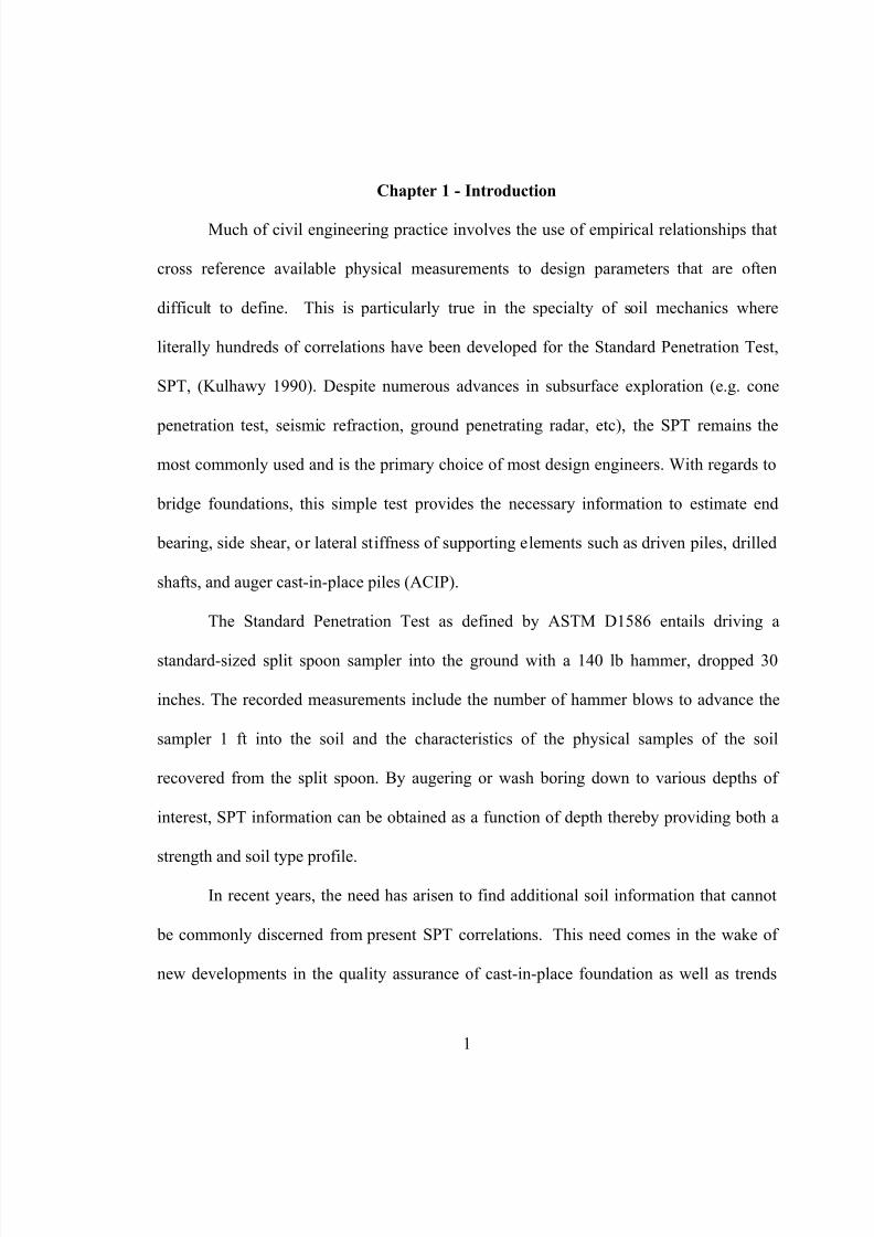
Chapter 1 - Introduction
Much of civil engineering practice involves the use of empirical relationships that
cross reference available physical measurements to design parameters that are often
difficult to define. This is particularly true in the specialty of soil mechanics where
literally hundreds of correlations have been developed for the Standard Penetration Test,
SPT, (Kulhawy 1990). Despite numerous advances in subsurface exploration (e.g. cone
penetration test, seismic refraction, ground penetrating radar, etc), the SPT remains themost commonly used and is the primary choice of most design engineers. With regards to
bridge foundations, this simple test provides the necessary information to estimate end
bearing, side shear, or lateral stiffness of supporting elements such as driven piles, drilled
shafts, and auger cast-in-place piles (ACIP).
The Standard Penetration Test as defined by ASTM D1586 entails driving a
standard-sized split spoon sampler into the ground with a 140 lb hammer, dropped 30
inches. The recorded measurements include the number of hammer blows to advance the
sampler 1 ft into the soil and the characteristics of the physical samples of the soil
recovered from the split spoon. By augering or wash boring down to various depths of
interest, SPT information can be obtained as a function of depth thereby providing both a
strength and soil type profile.
In recent years, the need has arisen to find additional soil information that cannot
be commonly discerned from present SPT correlations. This need comes in the wake of
new developments in the quality assurance of cast-in-place foundation as well as trends
8/16/2019 Thermal Conductivity of Soils From the Analysis of Boring Logs
http://slidepdf.com/reader/full/thermal-conductivity-of-soils-from-the-analysis-of-boring-logs 13/96
2
toward developing “greener” heating/cooling systems. In these cases, the ability of the soil
to diffuse or provide thermal energy can only be assessed by knowing the thermal
properties, specific heat and thermal conductivity, as well as ambient temperature
conditions.
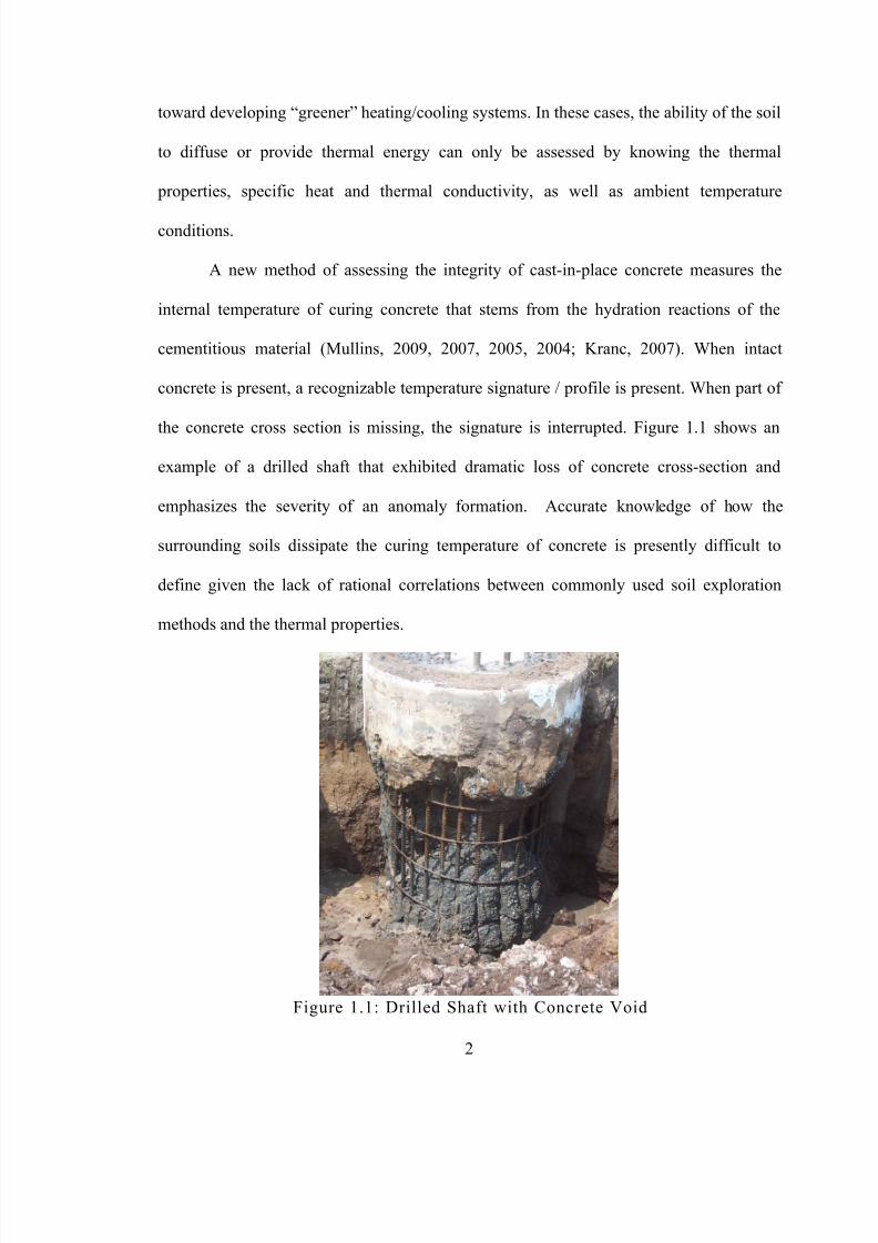
A new method of assessing the integrity of cast-in-place concrete measures the
internal temperature of curing concrete that stems from the hydration reactions of the
cementitious material (Mullins, 2009, 2007, 2005, 2004; Kranc, 2007). When intact
concrete is present, a recognizable temperature signature / profile is present. When part of
the concrete cross section is missing, the signature is interrupted. Figure 1.1 shows anexample of a drilled shaft that exhibited dramatic loss of concrete cross-section and
emphasizes the severity of an anomaly formation. Accurate knowledge of how the
surrounding soils dissipate the curing temperature of concrete is presently difficult to
define given the lack of rational correlations between commonly used soil exploration
methods and the thermal properties.
Figure 1.1: Drilled Shaft with Concrete Void
8/16/2019 Thermal Conductivity of Soils From the Analysis of Boring Logs
http://slidepdf.com/reader/full/thermal-conductivity-of-soils-from-the-analysis-of-boring-logs 14/96
3
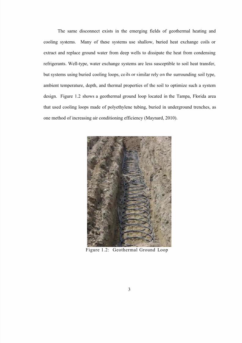
The same disconnect exists in the emerging fields of geothermal heating and
cooling systems. Many of these systems use shallow, buried heat exchange coils or
extract and replace ground water from deep wells to dissipate the heat from condensing
refrigerants. Well-type, water exchange systems are less susceptible to soil heat transfer,
but systems using buried cooling loops, coils or similar rely on the surrounding soil type,
ambient temperature, depth, and thermal properties of the soil to optimize such a system
design. Figure 1.2 shows a geothermal ground loop located in the Tampa, Florida area
that used cooling loops made of polyethylene tubing, buried in underground trenches, as
one method of increasing air conditioning efficiency (Maynard, 2010).
Figure 1.2: Geothermal Ground Loop
8/16/2019 Thermal Conductivity of Soils From the Analysis of Boring Logs
http://slidepdf.com/reader/full/thermal-conductivity-of-soils-from-the-analysis-of-boring-logs 15/96
4
Although the process used to install the polyethylene coils (as shown) disturbs the
natural state of the soil and the associated thermal properties (increasing or decreasing
density), the use of standard soil exploration methods would provide the system designer a
rationale for specifying a finished state or at least provide boundaries for the possible
range of thermal properties that are likely to result.
The focus of this study was to provide correlations between the boring log data from
the SPT test and thermal properties of the soils present in the boring log. To that end, an
Excel spreadsheet was created to take the blow counts and soil profile from the boring log
and use them to calculate the thermal conductivity at any depth based on published, predictive approaches. This was supplemented with thermal conductivity testing in the
laboratory to validate the results of the previously published relationships.
By calculating the thermal properties of soils, a better understanding of how the
surrounding soils react through the ground when hot water or liquid concrete is pumped
into it. The thermal conductivity and specific heat values of the soil will show how the
ground reacts to the heat that it is receiving, and how much of that heat can be stored. This
is especially helpful to the future of geotechnical engineering when designing geothermal
systems and analyzing the structural integrity of concrete drilled shafts.
1.1 Organization of Thesis
This thesis is organized into four ensuing chapters describing the background,
testing, results, and finally applications of the thesis findings with conclusions.
Chapter 2 outlines the historical evolution of the modern day understanding of
thermal properties of soil. This includes not only the testing and predictive efforts to
8/16/2019 Thermal Conductivity of Soils From the Analysis of Boring Logs
http://slidepdf.com/reader/full/thermal-conductivity-of-soils-from-the-analysis-of-boring-logs 16/96
5
define these properties, but also the applications that were instrumental in motivating
research to that end.
Chapter 3 provides the process for developing the algorithms used to design the
spreadsheet. Each component of the spreadsheet is broken down into a separate section
with a thorough explanation included for each. These provide the reader a step-by-step
overview of the process.
Chapter 4 discusses the testing and evaluation of thermal properties. The testing
section discusses the equipment used and procedures followed for the laboratory tests
conducted, along with the evaluation of these tests. This includes the recorded data,calculations, and an analysis of the results showing how the experimental data correlates
with published thermal conductivity values. Chapter 4 concludes with the evaluation of
the theoretical algorithms where a simple boring log is presented to aid as example of how
the spreadsheet functions.
Chapter 5 concludes the report by summarizing the results and solidifying the
correlation between boring log data and thermal properties. This chapter also provides
information on current applications and recommendations for future studies on this topic.
8/16/2019 Thermal Conductivity of Soils From the Analysis of Boring Logs
http://slidepdf.com/reader/full/thermal-conductivity-of-soils-from-the-analysis-of-boring-logs 17/96
6
Chapter 2 - Literature Review
A thorough literature review was conducted to initiate and focus the scope of this
thesis. The topics of this literature review include an overview of thermal properties and
usage, a history of thermal conductivity testing, standard soil testing methods, and existing
correlations defining the thermal properties of soils.
2.1 Overview
Thermal conductivity and specific heat are the primary parameters affecting the
transfer of heat energy through a given material. This transfer is commonly referred to as
conductive heat flow when it uses these parameters, but often mechanisms including
convection or radiation also contribute to the overall transfer, particularly in fluids or
gases. For solids or particulates, the conductive mechanism overwhelmingly controls.
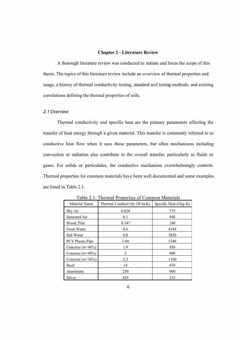
Thermal properties for common materials have been well documented and some examples
are listed in Table 2.1.
Table 2.1: Thermal Properties of Common MaterialsMaterial Name Thermal Conductivity (W/m-K) Specific Heat (J/kg-K)
Dry Air 0.024 775
Saturated Air 0.1 940
Wood, Pine 0.147 240
Fresh Water 0.6 4184
Salt Water 0.8 3850
PCV Plastic Pipe 1.04 1340
Concrete (w=44%) 1.9 850
Concrete (w=40%) 2 900
Concrete (w=36%) 2.3 1100
Steel 14 470
Aluminum 250 900
Silver 429 233
8/16/2019 Thermal Conductivity of Soils From the Analysis of Boring Logs
http://slidepdf.com/reader/full/thermal-conductivity-of-soils-from-the-analysis-of-boring-logs 18/96
7
Some values for soils can be found, but they vary widely in value likely caused by
being poorly defined. Variations in temperature, density, and moisture content directly
affect thermal properties making it difficult to accurately assess them without this
information.
The correlations between thermal and mechanical properties of soil particles have
been cited as being affected by close contact and density whereby thermo-elastic waves
transmit heat. Farouki (1966) translated this concept from Debye (1914) where heat flow
through a crystalline material occurs as warm atoms vibrate more than cooler atoms
causing waves to travel through the material proportional to bond strength between theatoms.
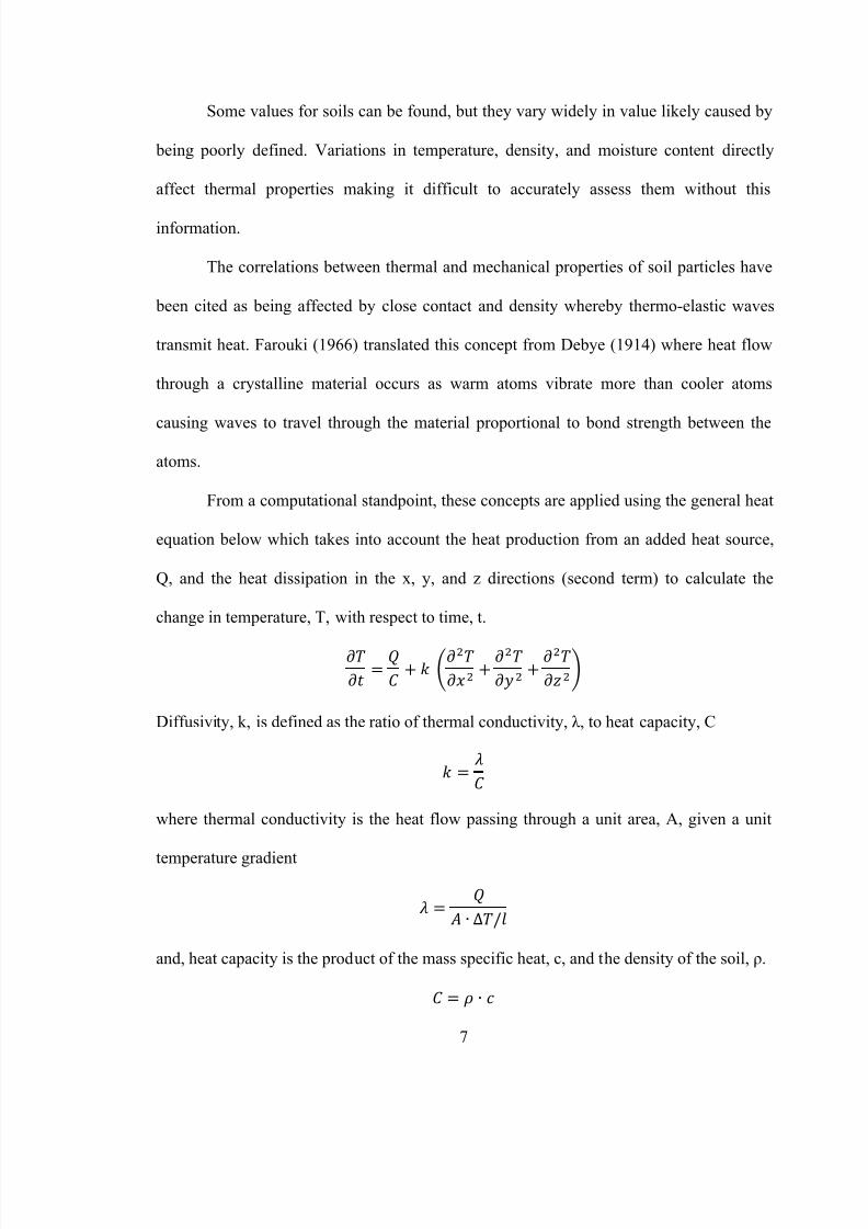
From a computational standpoint, these concepts are applied using the general heat
equation below which takes into account the heat production from an added heat source,
Q, and the heat dissipation in the x, y, and z directions (second term) to calculate the
change in temperature, T, with respect to time, t.
Diffusivity, k, is defined as the ratio of thermal conductivity, λ, to heat capacity, C
where thermal conductivity is the heat flow passing through a unit area, A, given a unit
temperature gradient
and, heat capacity is the product of the mass specific heat, c, and the density of the soil, ρ.
8/16/2019 Thermal Conductivity of Soils From the Analysis of Boring Logs
http://slidepdf.com/reader/full/thermal-conductivity-of-soils-from-the-analysis-of-boring-logs 19/96
8
In the application of geothermal heating/cooling systems, the source of heat is the
hot water or coolant from the H.V.A.C. heat exchanger and can be considered a relatively
constant heat flow for a given season. For shaft integrity applications, the heat source only
exists during concrete curing, after which the second term of the general heat equation
dominates the resultant temperature of the concrete.
2.2 Thermal Conductivity of Soil s (Background)
Thermal testing of standard construction materials such as wood, concrete, plaster,
and insulations are relatively straight forward when compared to soils. Until the late
1940’s, little research had been performed on the thermal conductivity of soils. At th at
time, Miles S. Kersten conducted a significant amount of research on this topic at the
University of Minnesota.
Studies were performed on 19 different soil types, consisting of a variety of sands,
gravels, sandy loams, clays, minerals, crushed rocks, and organics. To quantify the
thermal properties of these soils, numerous influential variables were identified including;
mineralogy, density, moisture content, and moisture state. The primary focus of this
research was to study the effects of the thermal conductivity of soils in permafrost regions
in order to address complications arising from construction in these regions. A strong
knowledge base of thermal properties was thought to help correct this problem (Kersten
1949).
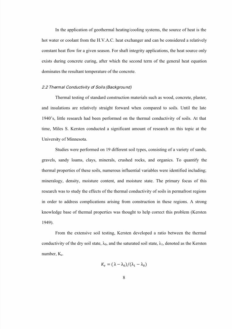
From the extensive soil testing, Kersten developed a ratio between the thermal
conductivity of the dry soil state, λ 0, and the saturated soil state , λ 1, denoted as the Kersten
number, K e.
8/16/2019 Thermal Conductivity of Soils From the Analysis of Boring Logs
http://slidepdf.com/reader/full/thermal-conductivity-of-soils-from-the-analysis-of-boring-logs 20/96
9
Kersten then developed empirical correlations between this number and the degree of
saturation, S r . For unfrozen soils, the Kersten number was defined as:
For frozen soils it is simply equal to the degree of saturation.
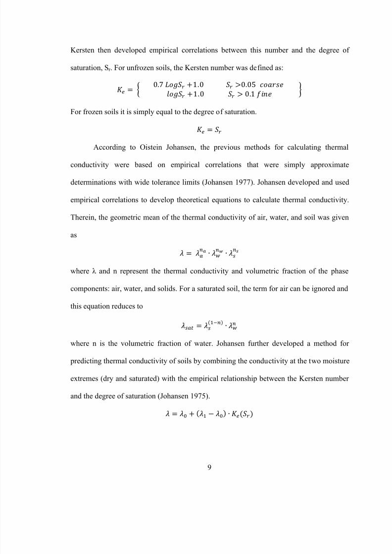
According to Oistein Johansen, the previous methods for calculating thermal
conductivity were based on empirical correlations that were simply approximate
determinations with wide tolerance limits (Johansen 1977). Johansen developed and used
empirical correlations to develop theoretical equations to calculate thermal conductivity.
Therein, the geometric mean of the thermal conductivity of air, water, and soil was given
as
where λ and n represent the thermal conductivity and volumetric fraction of the phase
components: air, water, and solids. For a saturated soil, the term for air can be ignored and
this equation reduces to
where n is the volumetric fraction of water. Johansen further developed a method for
predicting thermal conductivity of soils by combining the conductivity at the two moisture
extremes (dry and saturated) with the empirical relationship between the Kersten number
and the degree of saturation (Johansen 1975).
8/16/2019 Thermal Conductivity of Soils From the Analysis of Boring Logs
http://slidepdf.com/reader/full/thermal-conductivity-of-soils-from-the-analysis-of-boring-logs 21/96
10
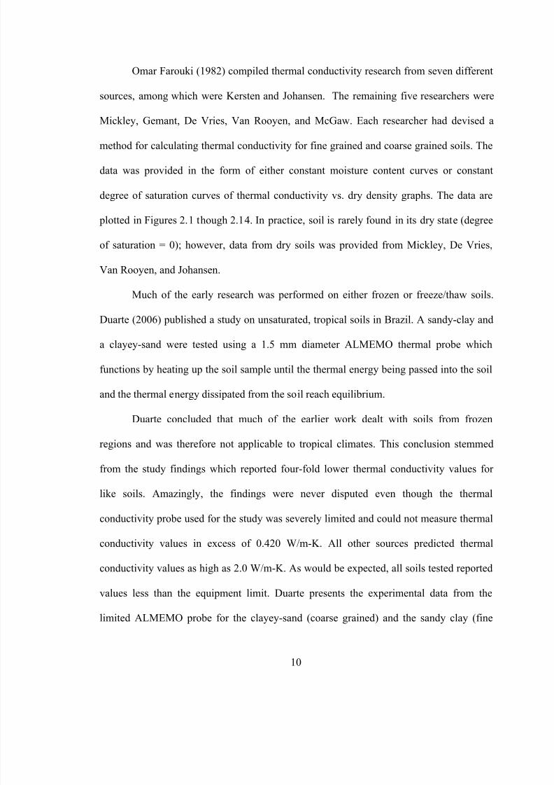
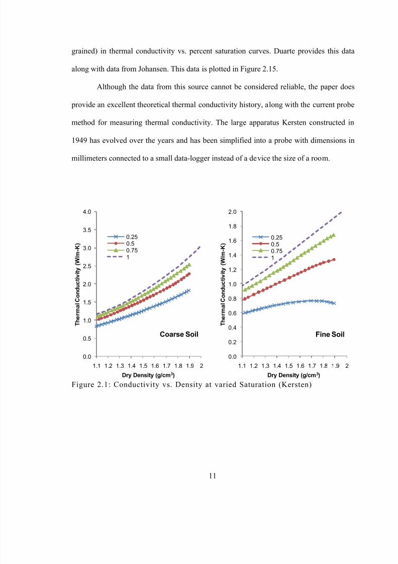
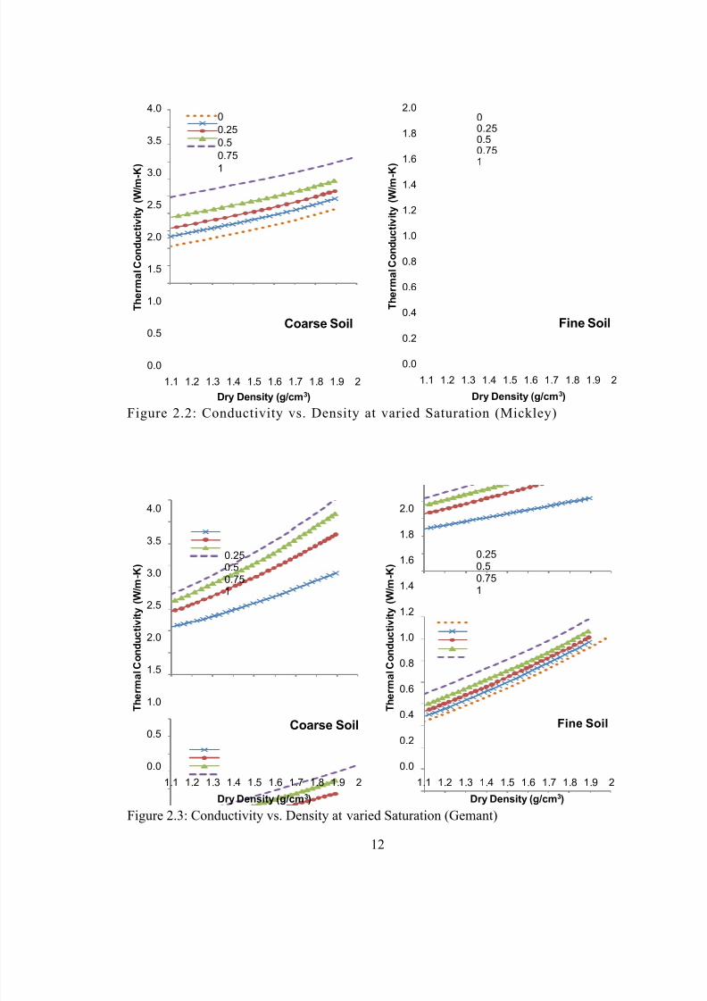
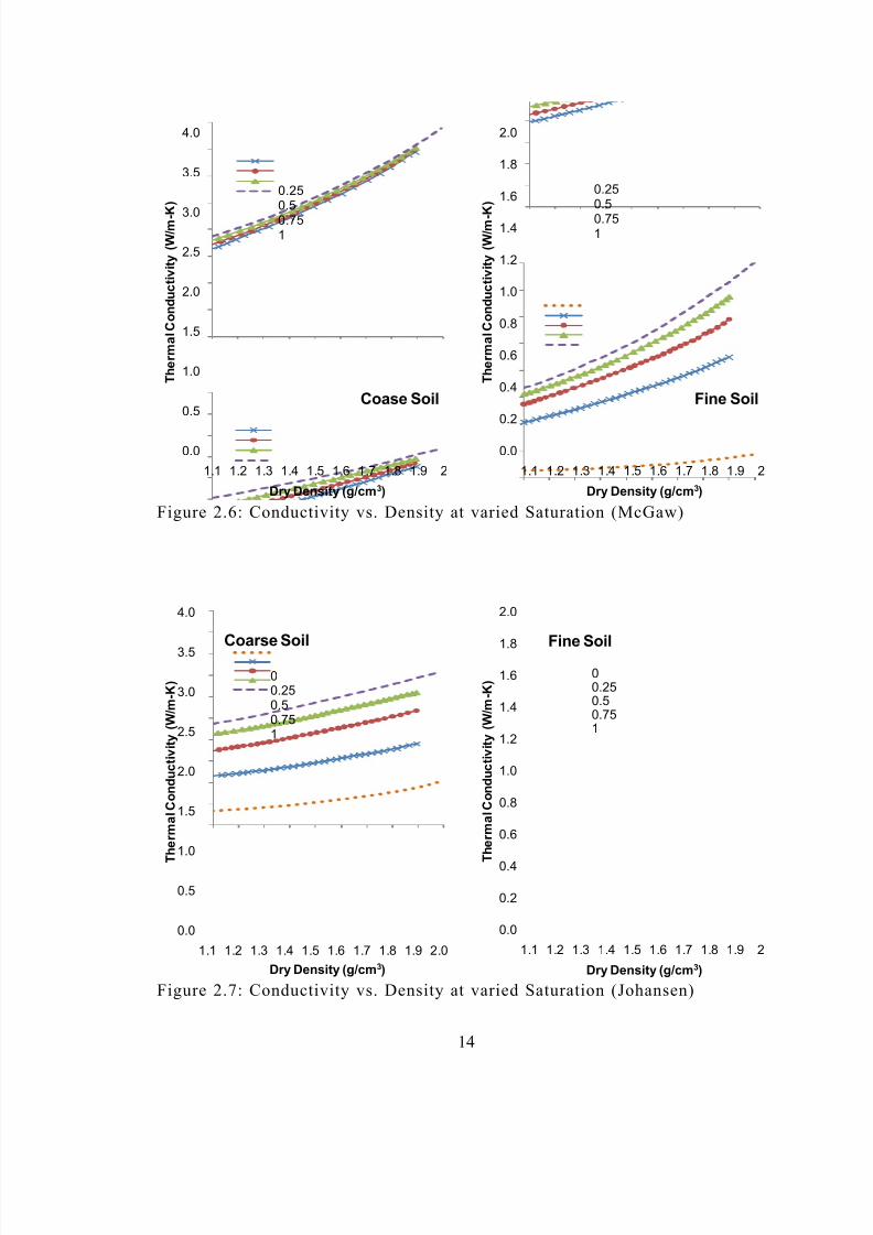
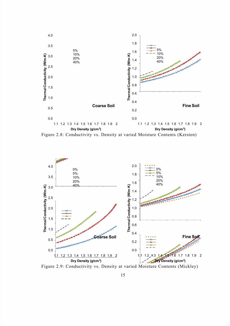
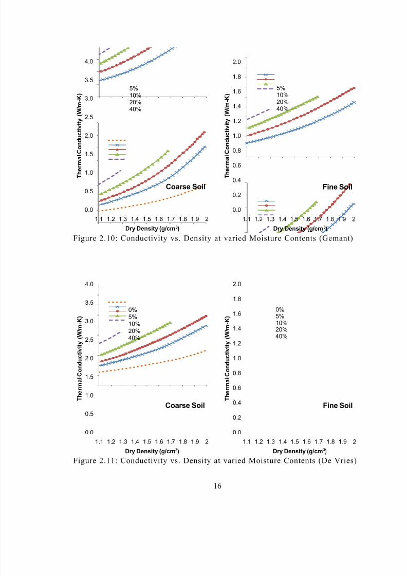
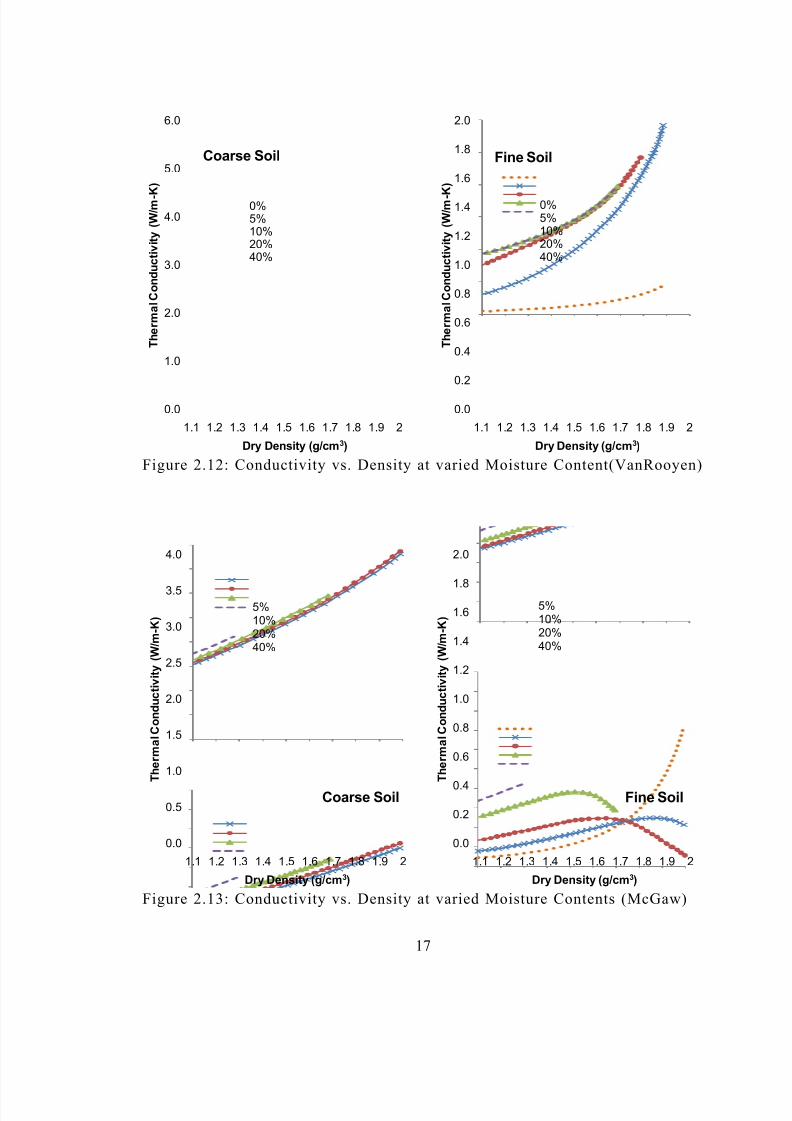
Omar Farouki (1982) compiled thermal conductivity research from seven different
sources, among which were Kersten and Johansen. The remaining five researchers were
Mickley, Gemant, De Vries, Van Rooyen, and McGaw. Each researcher had devised a
method for calculating thermal conductivity for fine grained and coarse grained soils. The
data was provided in the form of either constant moisture content curves or constant
degree of saturation curves of thermal conductivity vs. dry density graphs. The data are
plotted in Figures 2.1 though 2.14. In practice, soil is rarely found in its dry state (degree
of saturation = 0); however, data from dry soils was provided from Mickley, De Vries,
Van Rooyen, and Johansen.Much of the early research was performed on either frozen or freeze/thaw soils.
Duarte (2006) published a study on unsaturated, tropical soils in Brazil. A sandy-clay and
a clayey-sand were tested using a 1.5 mm diameter ALMEMO thermal probe which
functions by heating up the soil sample until the thermal energy being passed into the soil
and the thermal energy dissipated from the soil reach equilibrium.
Duarte concluded that much of the earlier work dealt with soils from frozen
regions and was therefore not applicable to tropical climates. This conclusion stemmed
from the study findings which reported four-fold lower thermal conductivity values for
like soils. Amazingly, the findings were never disputed even though the thermal
conductivity probe used for the study was severely limited and could not measure thermal
conductivity values in excess of 0.420 W/m-K. All other sources predicted thermal
conductivity values as high as 2.0 W/m-K. As would be expected, all soils tested reported
values less than the equipment limit. Duarte presents the experimental data from the
limited ALMEMO probe for the clayey-sand (coarse grained) and the sandy clay (fine
8/16/2019 Thermal Conductivity of Soils From the Analysis of Boring Logs
http://slidepdf.com/reader/full/thermal-conductivity-of-soils-from-the-analysis-of-boring-logs 22/96
11
grained) in thermal conductivity vs. percent saturation curves. Duarte provides this data
along with data from Johansen. This data is plotted in Figure 2.15.
Although the data from this source cannot be considered reliable, the paper does
provide an excellent theoretical thermal conductivity history, along with the current probe
method for measuring thermal conductivity. The large apparatus Kersten constructed in
1949 has evolved over the years and has been simplified into a probe with dimensions in
millimeters connected to a small data-logger instead of a device the size of a room.
Figure 2.1: Conductivity vs. Density at varied Saturation (Kersten)
0.0
0.5
1.0
1.5
2.0
2.5
3.0
3.5
4.0
1.1 1.2 1.3 1.4 1.5 1.6 1.7 1.8 1.9 2
T h e r m a l C o n d u c t i v i t y
( W / m - K
)
Dry Density (g/cm 3)
Coarse Soil
0.250.50.751
0.0
0.2
0.4
0.6
0.8
1.0
1.2
1.4
1.6
1.8
2.0
1.1 1.2 1.3 1.4 1.5 1.6 1.7 1.8 1.9 2
T h e r m a l C o n d u c t i v i t y
( W / m - K
)
Dry Density (g/cm 3)
Fine Soil
0.250.50.751
8/16/2019 Thermal Conductivity of Soils From the Analysis of Boring Logs
http://slidepdf.com/reader/full/thermal-conductivity-of-soils-from-the-analysis-of-boring-logs 23/96
12
Figure 2.2: Conductivity vs. Density at varied Saturation (Mickley)
Figure 2.3: Conductivity vs. Density at varied Saturation (Gemant)
0.0
0.5
1.0
1.5
2.0
2.5
3.0
3.5
4.0
1.1 1.2 1.3 1.4 1.5 1.6 1.7 1.8 1.9 2
T h e r m a l C o n d u c t i v i t y
( W / m - K )
Dry Density (g/cm 3)
Coarse Soil
00.250.50.751
0.0
0.2
0.4
0.6
0.8
1.0
1.2
1.4
1.6
1.8
2.0
1.1 1.2 1.3 1.4 1.5 1.6 1.7 1.8 1.9 2
T h e r m a l C o n d u c t i v i t y
( W / m - K )
Dry Density (g/cm 3)
Fine Soil
00.250.50.751
0.0
0.5
1.0
1.5
2.0
2.5
3.0
3.5
4.0
1.1 1.2 1.3 1.4 1.5 1.6 1.7 1.8 1.9 2
T h e r m a l C o n d u c t i v i t y
( W / m - K
)
Dry Density (g/cm 3)
Coarse Soil
0.250.50.751
0.0
0.2
0.4
0.6
0.8
1.0
1.2
1.4
1.6
1.8
2.0
1.1 1.2 1.3 1.4 1.5 1.6 1.7 1.8 1.9 2
T h e r m a l C o n d u c t i v i t y
( W / m - K
)
Dry Density (g/cm 3)
Fine Soil
0.250.50.751
8/16/2019 Thermal Conductivity of Soils From the Analysis of Boring Logs
http://slidepdf.com/reader/full/thermal-conductivity-of-soils-from-the-analysis-of-boring-logs 24/96
13
Figure 2.4: Conductivity vs. Density at varied Saturation (De Vries)
Figure 2.5: Conductivity vs. Density at varied Saturation (VanRooyen)
0.0
0.5
1.0
1.5
2.0
2.5
3.0
3.5
4.0
1.1 1.2 1.3 1.4 1.5 1.6 1.7 1.8 1.9 2
T h e r m a l C o n d u c t i v i t y
( W / m - K )
Dry Density (g/cm 3)
Coarse Soil
00.250.50.751
0.0
0.2
0.4
0.6
0.8
1.0
1.2
1.4
1.6
1.8
2.0
1.1 1.2 1.3 1.4 1.5 1.6 1.7 1.8 1.9 2
T h e r m a l C o n d u c t i v i t y
( W / m - K )
Dry Density (g/cm 3)
Fine Soil
00.25
0.50.751
0.0
1.0
2.0
3.0
4.0
5.0
6.0
1.1 1.2 1.3 1.4 1.5 1.6 1.7 1.8 1.9 2
T h e r m a l C o n d u c t i v i t y
( W / m - K
)
Dry Density (g/cm 3)
Coarse Soil
00.250.50.751
0.0
0.2
0.4
0.6
0.8
1.0
1.2
1.4
1.6
1.8
2.0
1.1 1.2 1.3 1.4 1.5 1.6 1.7 1.8 1.9 2
T h e r m a l C o n d u c t i v i t y
( W / m - K
)
Dry Density (g/cm 3)
Fine Soil
00.250.50.751
8/16/2019 Thermal Conductivity of Soils From the Analysis of Boring Logs
http://slidepdf.com/reader/full/thermal-conductivity-of-soils-from-the-analysis-of-boring-logs 25/96
14
Figure 2.6: Conductivity vs. Density at varied Saturation (McGaw)
Figure 2.7: Conductivity vs. Density at varied Saturation (Johansen)
0.0
0.5
1.0
1.5
2.0
2.5
3.0
3.5
4.0
1.1 1.2 1.3 1.4 1.5 1.6 1.7 1.8 1.9 2
T h e r m a l C o n d u c t i v i t y
( W / m - K )
Dry Density (g/cm 3)
Coase Soil
0.250.50.751
0.0
0.2
0.4
0.6
0.8
1.0
1.2
1.4
1.6
1.8
2.0
1.1 1.2 1.3 1.4 1.5 1.6 1.7 1.8 1.9 2
T h e r m a l C o n d u c t i v i t y
( W / m - K )
Dry Density (g/cm 3)
Fine Soil
0.250.50.751
0.0
0.5
1.0
1.5
2.0
2.5
3.0
3.5
4.0
1.1 1.2 1.3 1.4 1.5 1.6 1.7 1.8 1.9 2.0
T h e r m a l C o n d u c t i v i t y
( W / m - K
)
Dry Density (g/cm 3)
Coarse Soil
00.250.50.751
0.0
0.2
0.4
0.6
0.8
1.0
1.2
1.4
1.6
1.8
2.0
1.1 1.2 1.3 1.4 1.5 1.6 1.7 1.8 1.9 2
T h e r m a l C o n d u c t i v i t y
( W / m - K
)
Dry Density (g/cm 3)
Fine Soil00.250.50.751
8/16/2019 Thermal Conductivity of Soils From the Analysis of Boring Logs
http://slidepdf.com/reader/full/thermal-conductivity-of-soils-from-the-analysis-of-boring-logs 26/96
15
Figure 2.8: Conductivity vs. Density at varied Moisture Contents (Kersten)
Figure 2.9: Conductivity vs. Density at varied Moisture Contents (Mickley)
0.0
0.5
1.0
1.5
2.0
2.5
3.0
3.5
4.0
1.1 1.2 1.3 1.4 1.5 1.6 1.7 1.8 1.9 2
T h e r m a l C o n d u c t i v i t y
( W / m - K )
Dry Density (g/cm 3)
Coarse Soil
5%10%20%40%
0.0
0.2
0.4
0.6
0.8
1.0
1.2
1.4
1.6
1.8
2.0
1.1 1.2 1.3 1.4 1.5 1.6 1.7 1.8 1.9 2
T h e r m a l C o n d u c t i v i t y
( W / m - K )
Dry Density (g/cm 3)
Fine Soil
5%10%20%40%
0.0
0.5
1.0
1.5
2.0
2.5
3.0
3.5
4.0
1.1 1.2 1.3 1.4 1.5 1.6 1.7 1.8 1.9 2
T h e r m a l C o n d u c t i v i t y
( W / m - K
)
Dry Density (g/cm 3)
Coarse Soil
0%5%10%20%40%
0.0
0.2
0.4
0.6
0.8
1.0
1.2
1.4
1.6
1.8
2.0
1.1 1.2 1.3 1.4 1.5 1.6 1.7 1.8 1.9 2
T h e r m a l C o n d u c t i v i t y
( W / m - K
)
Dry Density (g/cm 3)
Fine Soil
0%5%10%20%40%
8/16/2019 Thermal Conductivity of Soils From the Analysis of Boring Logs
http://slidepdf.com/reader/full/thermal-conductivity-of-soils-from-the-analysis-of-boring-logs 27/96
16
Figure 2.10: Conductivity vs. Density at varied Moisture Contents (Gemant)
Figure 2.11: Conductivity vs. Density at varied Moisture Contents (De Vries)
0.0
0.5
1.0
1.5
2.0
2.5
3.0
3.5
4.0
1.1 1.2 1.3 1.4 1.5 1.6 1.7 1.8 1.9 2
T h e r m a l C o n d u c t i v i t y
( W / m - K )
Dry Density (g/cm 3)
Coarse Soil
5%10%20%40%
0.0
0.2
0.4
0.6
0.8
1.0
1.2
1.4
1.6
1.8
2.0
1.1 1.2 1.3 1.4 1.5 1.6 1.7 1.8 1.9 2
T h e r m a l C o n d u c t i v i t y
( W / m - K )
Dry Density (g/cm 3)
Fine Soil
5%10%20%40%
0.0
0.5
1.0
1.5
2.0
2.5
3.0
3.5
4.0
1.1 1.2 1.3 1.4 1.5 1.6 1.7 1.8 1.9 2
T h e r m a l C o n d u c t i v i t y
( W / m - K
)
Dry Density (g/cm 3)
Coarse Soil
0%5%10%20%40%
0.0
0.2
0.4
0.6
0.8
1.0
1.2
1.4
1.6
1.8
2.0
1.1 1.2 1.3 1.4 1.5 1.6 1.7 1.8 1.9 2
T h e r m a l C o n d u c t i v i t y
( W / m - K
)
Dry Density (g/cm 3)
Fine Soil
0%5%10%20%40%
8/16/2019 Thermal Conductivity of Soils From the Analysis of Boring Logs
http://slidepdf.com/reader/full/thermal-conductivity-of-soils-from-the-analysis-of-boring-logs 28/96
17
Figure 2.12: Conductivity vs. Density at varied Moisture Content(VanRooyen)
Figure 2.13: Conductivity vs. Density at varied Moisture Contents (McGaw)
0.0
1.0
2.0
3.0
4.0
5.0
6.0
1.1 1.2 1.3 1.4 1.5 1.6 1.7 1.8 1.9 2
T h e r m a l C o n d u c t i v i t y
( W / m - K )
Dry Density (g/cm 3)
Coarse Soil
0%5%10%20%40%
0.0
0.2
0.4
0.6
0.8
1.0
1.2
1.4
1.6
1.8
2.0
1.1 1.2 1.3 1.4 1.5 1.6 1.7 1.8 1.9 2
T h e r m a l C o n d u c t i v i t y
( W / m - K )
Dry Density (g/cm 3)
Fine Soil
0%5%10%20%40%
0.0
0.5
1.0
1.5
2.0
2.5
3.0
3.5
4.0
1.1 1.2 1.3 1.4 1.5 1.6 1.7 1.8 1.9 2
T h e r m a l C o n d u c t i v i t y
( W / m - K
)
Dry Density (g/cm 3)
Coarse Soil
5%10%20%40%
0.0
0.2
0.4
0.6
0.8
1.0
1.2
1.4
1.6
1.8
2.0
1.1 1.2 1.3 1.4 1.5 1.6 1.7 1.8 1.9 2
T h e r m a l C o n d u c t i v i t y
( W / m - K
)
Dry Density (g/cm 3)
Fine Soil
5%10%20%40%
8/16/2019 Thermal Conductivity of Soils From the Analysis of Boring Logs
http://slidepdf.com/reader/full/thermal-conductivity-of-soils-from-the-analysis-of-boring-logs 29/96
8/16/2019 Thermal Conductivity of Soils From the Analysis of Boring Logs
http://slidepdf.com/reader/full/thermal-conductivity-of-soils-from-the-analysis-of-boring-logs 30/96
19
2.3 Propert ies and M easur ement Corr elations
2.3.1 Boring Log Measurements
A boring log is a compilation of the data from a Standard Penetration Test. Boring
logs display blow count and soil type as a function of depth and often include moisture
content information for fine grain or clayey soils. The soil extracted from the split-spoon
sampler at each depth is placed in jars and taken to a laboratory to be classified using the
USCS standards to identify the soil type as well as moisture content.
2.3.2 Density
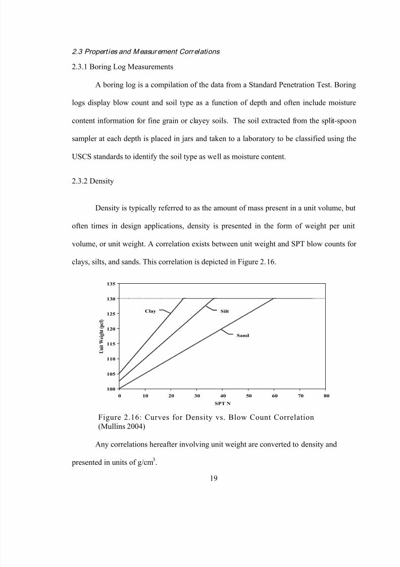
Density is typically referred to as the amount of mass present in a unit volume, but
often times in design applications, density is presented in the form of weight per unit
volume, or unit weight. A correlation exists between unit weight and SPT blow counts for
clays, silts, and sands. This correlation is depicted in Figure 2.16.
Figure 2.16: Curves for Density vs. Blow Count Correlation(Mullins 2004)
Any correlations hereafter involving unit weight are converted to density and
presented in units of g/cm 3.
100
105
110
115
120
125
130
135
0 10 20 30 40 50 60 70 80SPT N
U n i t W e i g h t ( p c f )
Clay Silt
Sand
8/16/2019 Thermal Conductivity of Soils From the Analysis of Boring Logs
http://slidepdf.com/reader/full/thermal-conductivity-of-soils-from-the-analysis-of-boring-logs 31/96
20
2.3.3 Moisture Content
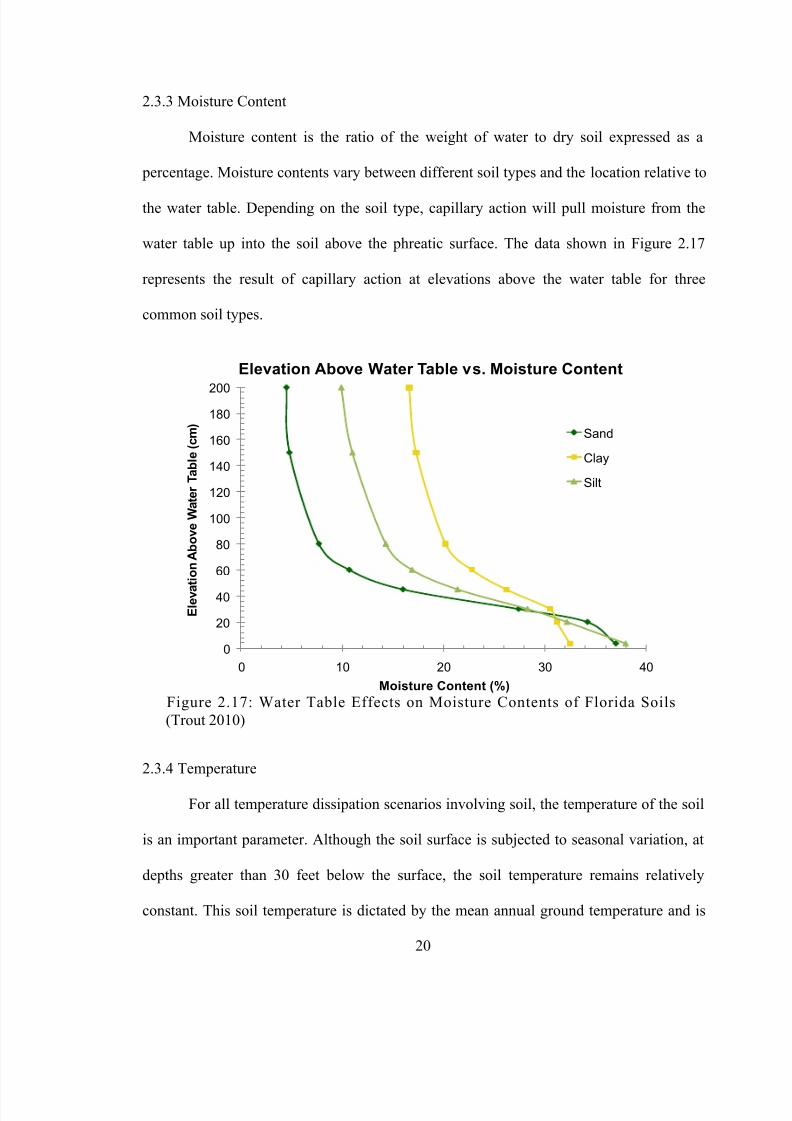
Moisture content is the ratio of the weight of water to dry soil expressed as a
percentage. Moisture contents vary between different soil types and the location relative to
the water table. Depending on the soil type, capillary action will pull moisture from the
water table up into the soil above the phreatic surface. The data shown in Figure 2.17
represents the result of capillary action at elevations above the water table for three
common soil types.
Figure 2.17: Water Table Effects on Moisture Contents of Florida Soils(Trout 2010)
2.3.4 Temperature
For all temperature dissipation scenarios involving soil, the temperature of the soil
is an important parameter. Although the soil surface is subjected to seasonal variation, at
depths greater than 30 feet below the surface, the soil temperature remains relatively
constant. This soil temperature is dictated by the mean annual ground temperature and is
0
20
40
60
80
100
120
140
160
180200
0 10 20 30 40
E l e v a t i o n A b o v e
W a t e r
T a b l e ( c m )
Moisture Content (%)
Elevation Above Water Table vs. Moisture Content
Sand
Clay
Silt
8/16/2019 Thermal Conductivity of Soils From the Analysis of Boring Logs
http://slidepdf.com/reader/full/thermal-conductivity-of-soils-from-the-analysis-of-boring-logs 32/96
21
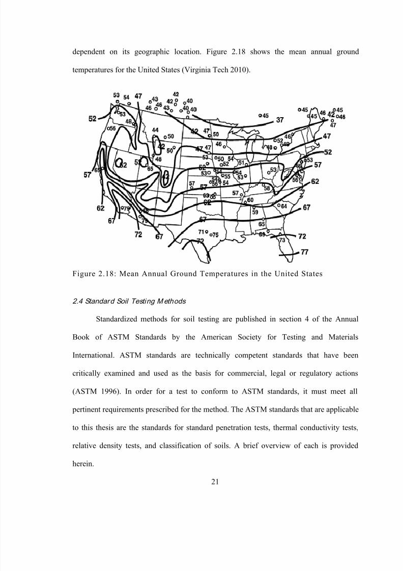
dependent on its geographic location. Figure 2.18 shows the mean annual ground
temperatures for the United States (Virginia Tech 2010).
Figure 2.18: Mean Annual Ground Temperatures in the United States
2.4 Standard Soil Testing M ethods
Standardized methods for soil testing are published in section 4 of the Annual
Book of ASTM Standards by the American Society for Testing and Materials
International. ASTM standards are technically competent standards that have been
critically examined and used as the basis for commercial, legal or regulatory actions
(ASTM 1996). In order for a test to conform to ASTM standards, it must meet all
pertinent requirements prescribed for the method. The ASTM standards that are applicable
to this thesis are the standards for standard penetration tests, thermal conductivity tests,
relative density tests, and classification of soils. A brief overview of each is provided
herein.
8/16/2019 Thermal Conductivity of Soils From the Analysis of Boring Logs
http://slidepdf.com/reader/full/thermal-conductivity-of-soils-from-the-analysis-of-boring-logs 33/96
22
2.4.1 Standard Penetration Test
The standard penetration test (briefly discussed in Chapter 1) consists of a split-
barrel sampler which is driven into the ground to obtain a soil sample. The resistance of
the soil to the penetration of the sampler, referred to as a blow count or SPT N, represents
the number of hammer blows necessary to advance the sampler 1 ft. The procedure for the
SPT test is outlined in ASTM D1586, the Standard Test Method for the Penetration Test
and Split-barrel Sampling of Soils. This test is conducted to provide a soil sample for
laboratory soil classification tests. The SPT N value can be correlated to a variety of
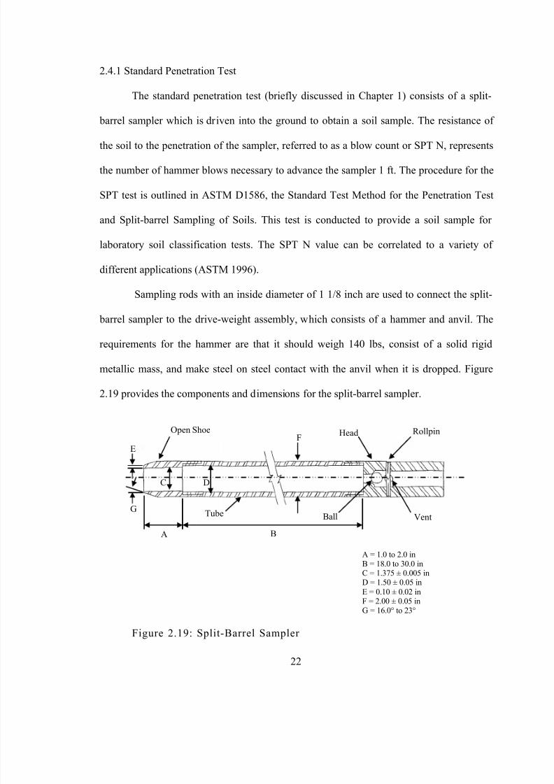
different applications (ASTM 1996).Sampling rods with an inside diameter of 1 1/8 inch are used to connect the split-
barrel sampler to the drive-weight assembly, which consists of a hammer and anvil. The
requirements for the hammer are that it should weigh 140 lbs, consist of a solid rigid
metallic mass, and make steel on steel contact with the anvil when it is dropped. Figure
2.19 provides the components and dimensions for the split-barrel sampler.
Figure 2.19: Split-Barrel Sampler
A = 1.0 to 2.0 inB = 18.0 to 30.0 inC = 1.375 ± 0.005 inD = 1.50 ± 0.05 inE = 0.10 ± 0.02 inF = 2.00 ± 0.05 inG = 16.0° to 23°
Open Shoe
Tube Ball
Head Rollpin
Vent
A
F
B
C D
E
G
8/16/2019 Thermal Conductivity of Soils From the Analysis of Boring Logs
http://slidepdf.com/reader/full/thermal-conductivity-of-soils-from-the-analysis-of-boring-logs 34/96
23
Once a boring has been advanced to desired elevation, the split-barrel sampler is
attached to the sampling rods and lowered into the hole. The drive-weight is then
positioned above and the anvil is attached to the sampling rods. The dead weight of the
sampler, rods, anvil and drive weight are rested on the bottom of the boring and a seating
blow is applied. The hammer is continuously dropped and the blows are counted over
three increments of 6 inches. The sampler is to be tested over the entire 18 inches unless
the soil is dense enough such that 50 blows have been applied over any 6 inch test, a total
of 100 blows have been applied, or there is no noticeable advance during the application
of 10 blows.When compiling the data into a boring log, the first 6 inches is referred to as the
seating drive and those blows are omitted. The blow counts of the second and third 6 inch
penetrations are summed to provide the number of blow counts from that test. If 6 inches
has not been reached within 50 blows, the blows per number of inches penetrated are
recorded.
2.4.2 Thermal Conductivity Testing
Methods for measuring thermal conductivity include the transient method and the
steady state method, the first of which is the most common. The Standard Test Method for
Determination of Thermal Conductivity of Soil and Soft Rock by Thermal Needle Probe,
ASTM D5334, is the approved transient heat method for thermal conductivity testing of
soils. This method is approved for use in both wet and dry soils, but as moisture increases,
percent error increases. Moisture can cause errors in the readings from the redistribution of
water due to thermal gradients resulting from heating of the probe (ASTM 2008). This
8/16/2019 Thermal Conductivity of Soils From the Analysis of Boring Logs
http://slidepdf.com/reader/full/thermal-conductivity-of-soils-from-the-analysis-of-boring-logs 35/96
24
error increases with greater heating times; therefore, either total heat added should be
minimized or heating time should be reduced for soils with high moisture contents.
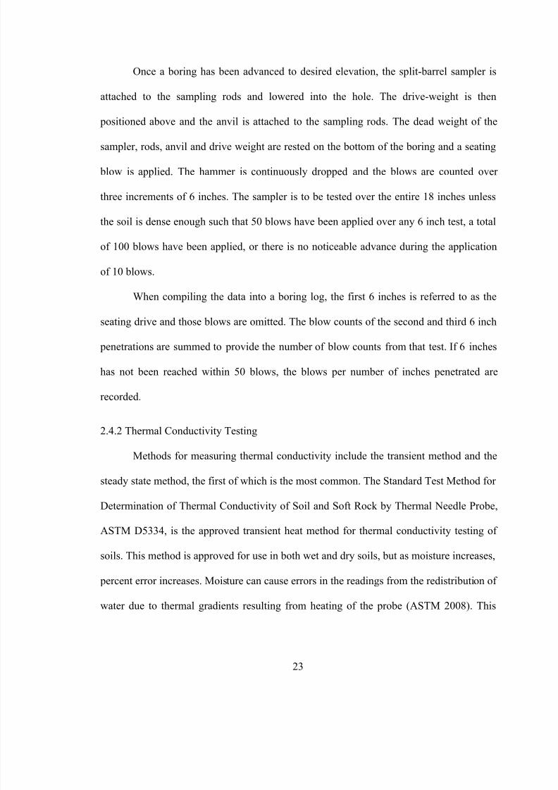
The equipment required for the test is a thermal needle probe, a constant current
source, a multimeter, and a data collection device that collects both temperature and time
readings. A probe with a large length to diameter ratio is required to simulate an infinitely
thin heating source. The typical probe design consists of a copper-constantan
thermocouple and either manganin or nichrome wire for the heating element encased in a
stainless steel or similar thin-walled, closed-end tube. The heating element connects to a
circuit with a constant current source which generates heat in the probe from the wireresistance when energized. The thermocouple wires are connected to the data collection
device which monitors the temperature changes over time. The typical probe design
according to ASTM 5334-08 is depicted in Figure 2.20.
Figure 2.20: ASTM D5334-08 – Typical Probe Components
ThermocoupleJack
CU CN
DC Heat Source
Heating Element - Nichrome orManganin Heating Wire
Copper
Constantan
E ox Ti
Epoxy Filled
Thermocouple Junction
8/16/2019 Thermal Conductivity of Soils From the Analysis of Boring Logs
http://slidepdf.com/reader/full/thermal-conductivity-of-soils-from-the-analysis-of-boring-logs 36/96
25
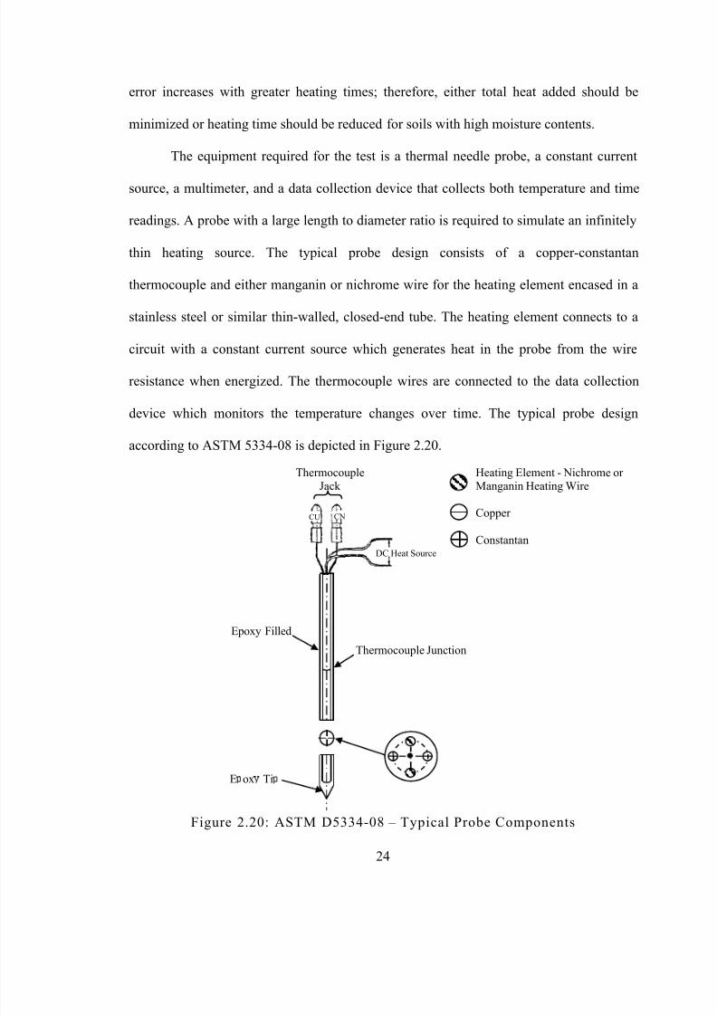
When conducting tests, known amounts of current and voltage are applied to the
probe and temperature rises are recorded over a period of time. A minimum of 20 to 30
readings should be recorded for each test. Once the data is collected, temperature is plotted
versus time on a semi-log time scale and the linear, steady-state portion of the curve is
selected. The slope of this portion of the temperature vs. time curve is used to calculate the
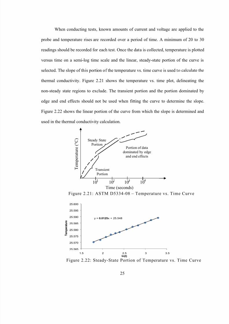
thermal conductivity. Figure 2.21 shows the temperature vs. time plot, delineating the
non-steady state regions to exclude. The transient portion and the portion dominated by
edge and end effects should not be used when fitting the curve to determine the slope.
Figure 2.22 shows the linear portion of the curve from which the slope is determined andused in the thermal conductivity calculation.
Figure 2.21: ASTM D5334-08 – Temperature vs. Time Curve
Figure 2.22: Steady-State Portion of Temperature vs. Time Curve
y = 0.0125 x + 25.548
25.565
25.570
25.575
25.580
25.585
25.590
25.595
25.600
1.5 2 2.5 3 3.5
T e m p e r a t u r e
ln(t)
Time (seconds)10 10 1010
T e m p e r a t u r e
( ° C )
Steady StatePortion
TransientPortion
Portion of datadominated by edge
and end effects
8/16/2019 Thermal Conductivity of Soils From the Analysis of Boring Logs
http://slidepdf.com/reader/full/thermal-conductivity-of-soils-from-the-analysis-of-boring-logs 37/96
26
Thermal conductivity is determined from the slope of the temperature vs. time
graph, S, the heat input, Q, and the calibration factor of the probe, C
where the heat input is the product of the current, I, and the voltage, V, divided by the
length of the probe, L.
2.4.3 Relative Density Test
The Standard Test Method for Maximum Index density and Unit Weight of Soils
Using a Vibratory Table, ASTM D4253, is used to determine the density index for
cohesionless, free-draining soils. This test is typically done to evaluate the state of
compactness of a soil sample. Two procedures, one for dry soils and one for wet soils, are
outlined in this standard. For this test to be applicable, 100 percent of the soil sample must
pass a 3 in sieve and at most, 15 percent of it can pass the No. 200 sieve. Regardless of the
percent fines, if the soil does not have the characteristics of a cohesionless, free-draining
soil, it does not meet ASTM standards for this test.
The testing apparatus comprises a vibrating table and mold assembly. The mold
assembly consists of the mold, the guide sleeve, the surcharge weight, the surcharge base-
plate, and the dial gage holder and indicator. Two standard mold options are available; the
0.1 ft 3 and the 0.5 ft 3 mold. Each mold has a specifically sized guide sleeve, weight, and
base-plate. To assemble the components, the mold is first attached to the table and the
surcharge base-plate is place on top. The guide sleeve is then attached to mold, and the
8/16/2019 Thermal Conductivity of Soils From the Analysis of Boring Logs
http://slidepdf.com/reader/full/thermal-conductivity-of-soils-from-the-analysis-of-boring-logs 38/96
27
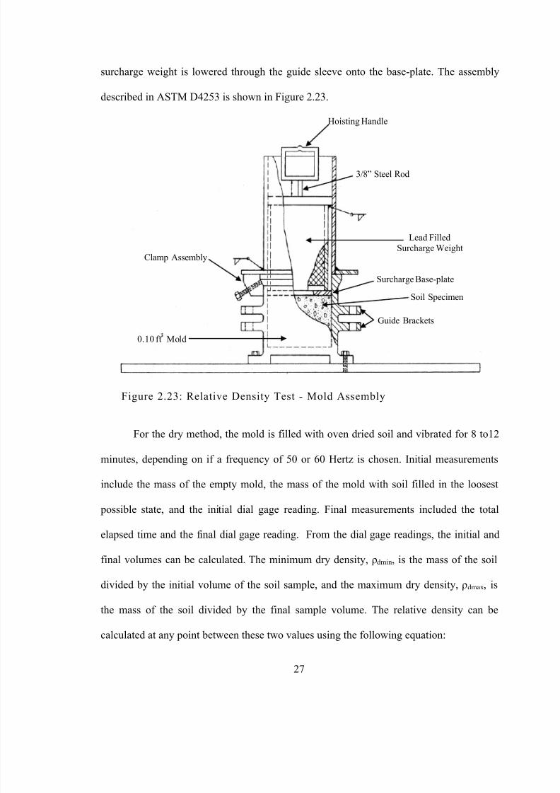
surcharge weight is lowered through the guide sleeve onto the base-plate. The assembly
described in ASTM D4253 is shown in Figure 2.23.
Figure 2.23: Relative Density Test - Mold Assembly
For the dry method, the mold is filled with oven dried soil and vibrated for 8 to12
minutes, depending on if a frequency of 50 or 60 Hertz is chosen. Initial measurements
include the mass of the empty mold, the mass of the mold with soil filled in the loosest
possible state, and the initial dial gage reading. Final measurements included the total
elapsed time and the final dial gage reading. From the dial gage readings, the initial and
final volumes can be calculated. The minimum dry density, ρ dmin , is the mass of the soil
divided by the initial volume of the soil sample, and the maximum dry density, ρ dmax , is
the mass of the soil divided by the final sample volume. The relative density can be
calculated at any point between these two values using the following equation:
Hoisting Handle
0.10 ft Mold
Guide Brackets
Soil Specimen
Surcharge Base-plate
Lead FilledSurcharge Weight
3/8” Steel Rod
Clamp Assembly
8/16/2019 Thermal Conductivity of Soils From the Analysis of Boring Logs
http://slidepdf.com/reader/full/thermal-conductivity-of-soils-from-the-analysis-of-boring-logs 39/96
28
The only variation between the dry and wet methods is that for the wet method, the
mold is initially attached to the table and wet soil is gently placed in it over a period of 5
to 6 minutes while the table is vibrating. This is done prior to attaching the guide sleeve,
base-plate, and weight to the mold. Because the mold is already bolted to the table when
the soil is placed in it, the mold and soil must be dried and weighed at the end of test.
2.4.4 Soil Classification
The Unified Soil Classification System (USCS) is presented in ASTM D2487, the
Standard for the Classification of Soils for Engineering Purposes. This standard classifies
soils into groups based on their particle size characteristics, liquid limit, and plasticity
index.
Soils are classified into four main groups: gravel (G), sand (S), silt (M), and clay
(C). Gravel and sand are classified as coarse-grained soils, while silt and clay are
classified as fine-grained. To be considered coarse-grained, at least 50 percent of the soil
mass must be retained on the No. 200 sieve, while 50 percent has to pass the No. 200 sieve
to be considered fine-grained. Gravels and sands are separated by the No. 4 sieve. If the
soil is retained on the No. 4 sieve, it is classified as a gravel whereas if it passes the No. 4
sieve and is retained on the No. 200, it is classified as a sand. Silts and clays require
additional tests before they can be classified. These tests are provided in ASTM D4318.
To classify a soil sample, a particle size distribution must be obtained. This entails
performing a sieve analysis for the entire soil sample using a series of sieves which should
include the 3 in, No. 4, and No. 200 sieves, along with several others. The soil sample is
weighed and sieved. Each sieve is weighed and the weight retained is recorded. Using the
8/16/2019 Thermal Conductivity of Soils From the Analysis of Boring Logs
http://slidepdf.com/reader/full/thermal-conductivity-of-soils-from-the-analysis-of-boring-logs 40/96
29
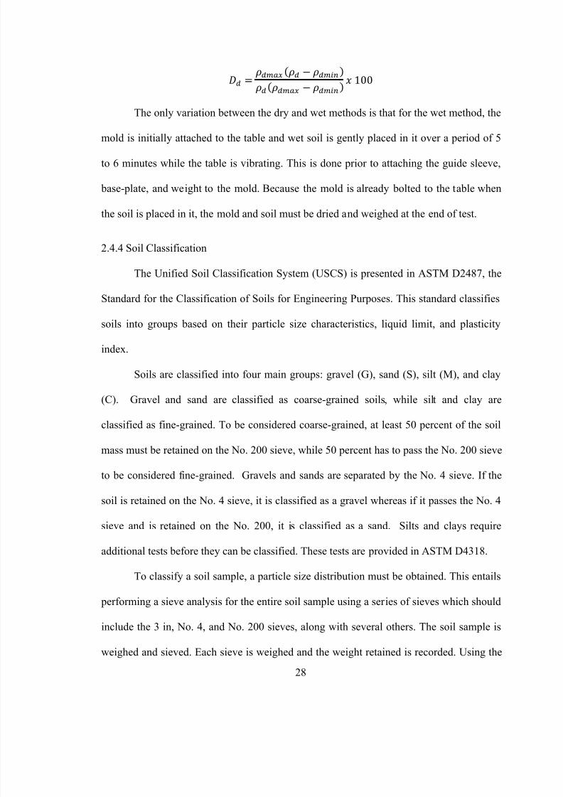
weight retained, the weight passing and the percent passing each sieve is calculated. For
fine-grained soils, the liquid limit and plastic limit must be determined. Once this
information is know, the USCS classification chart can be followed to classify the soil.
The USCS classification chart is provided in Table 2.2.
Table 2.2: USCS Soil Classification Chart
2.4.5 Thermal Integrity Profiling
The Thermal Integrity Profiler uses the temperature generated by curing cement
(hydration energy) to assess the quality of cast in place concrete foundations (i.e. drilled
shafts or ACIP piles). Whereas other methods of integrity testing are limited to specific
regions of the foundation cross-section (e.g. inside the reinforcing cage, between tubes, or
within a few inches of an access tube), TIP measurements are sensitive to the concrete
quality from all portions of the cross-section.
Group Symbol Group Name
GW Well-graded gravel
GP Poorly-graded gravel
GM Silty gravel
GC Clayey gravel
SW Well-graded sandSP Poorly-graded sand
SM Silty sand
SC Clayey sand
ML Silt
CL Lean clay
OL Low plasticity Organic silts and clays
MH Elastic Silt
CH Fat clay
OH High plasticity Organic silts and clays
PT Peat
Criteria for Assigning Group Symbols and Names
Gravels50% or more
retained on No. 4sieve
Sands50% or more
passes the No. 4sieve
Silts and Claysliquid limit less than 50
Silts and Claysliquid limit 50 or more
Coarse-Grained SoilsMore than 50% retained on
No. 200 sieve
Fine-Grained Soils50% or more passes
No. 200 sieve
Highly Organic Soils
Clean Gravels
Gravels withFine
Clean Sands
Sands withFines
8/16/2019 Thermal Conductivity of Soils From the Analysis of Boring Logs
http://slidepdf.com/reader/full/thermal-conductivity-of-soils-from-the-analysis-of-boring-logs 41/96
30
In general, the absence of intact / competent concrete is registered by relative cool
regions (necks or inclusions); the presence of additional / extra concrete is registered by
relative warm regions (over-pour bulging into soft soil strata). Anomalies both inside and
outside the reinforcing cage not only disrupt the normal temperature signature for the
nearest access tube, but the entire shaft; anomalies (inclusions, necks, bulges, etc.) are also
detected by more distal tubes (but with progressively less effect).
Analysis of the data has multiple levels of intricacy, but in general it depends on
the concrete mix design, shape, and geometry of the concrete tested as well as the
diffusion field (e.g. air, soil, water). As a result, the thermal properties of the soilsurrounding the concrete structure are important and form one focus of this thesis.
8/16/2019 Thermal Conductivity of Soils From the Analysis of Boring Logs
http://slidepdf.com/reader/full/thermal-conductivity-of-soils-from-the-analysis-of-boring-logs 42/96
31
Chapter 3 - Algorithm Development
The primary focus of this thesis was to provide design parameters for engineering
problems requiring thermal properties of soils. As the most common soil exploration
methodology involves SPT borings, a concentrated effort was put forth to relate both
thermal conductivity and specific heat to this form of soil data. To that end, presently
available correlations between SPT (N) and density were employed along with
correlations from density to thermal conductivity. This chapter provides detaileddevelopment of such algorithms to correlate the link between SPT (N) to thermal
properties.
An Excel spreadsheet was created using correlations where the data from a SPT
boring log could be inputted and these thermal properties could be calculated. The
necessary input data for the spreadsheet consists of depth, soil type, blow count, ground
surface elevation and the elevation of the water table. Ground surface elevation and water
table elevation are both single entry inputs, whereas depth, blow count, and soil type are
arrays requiring multiple entries for each field. Using these inputs, the soil structure,
moisture content, and density can be properly assigned. Once these values are known, the
thermal conductivity calculations are simply determined from a series of polynomial
equations. The parameters listed above are the deciding factors on which one of these
equations should be used for each entry.
Boring logs are provided in terms of either depth or elevation. Both are acceptable,
but depth was chosen as the input parameter for this spreadsheet. To provide the elevation
8/16/2019 Thermal Conductivity of Soils From the Analysis of Boring Logs
http://slidepdf.com/reader/full/thermal-conductivity-of-soils-from-the-analysis-of-boring-logs 43/96
32
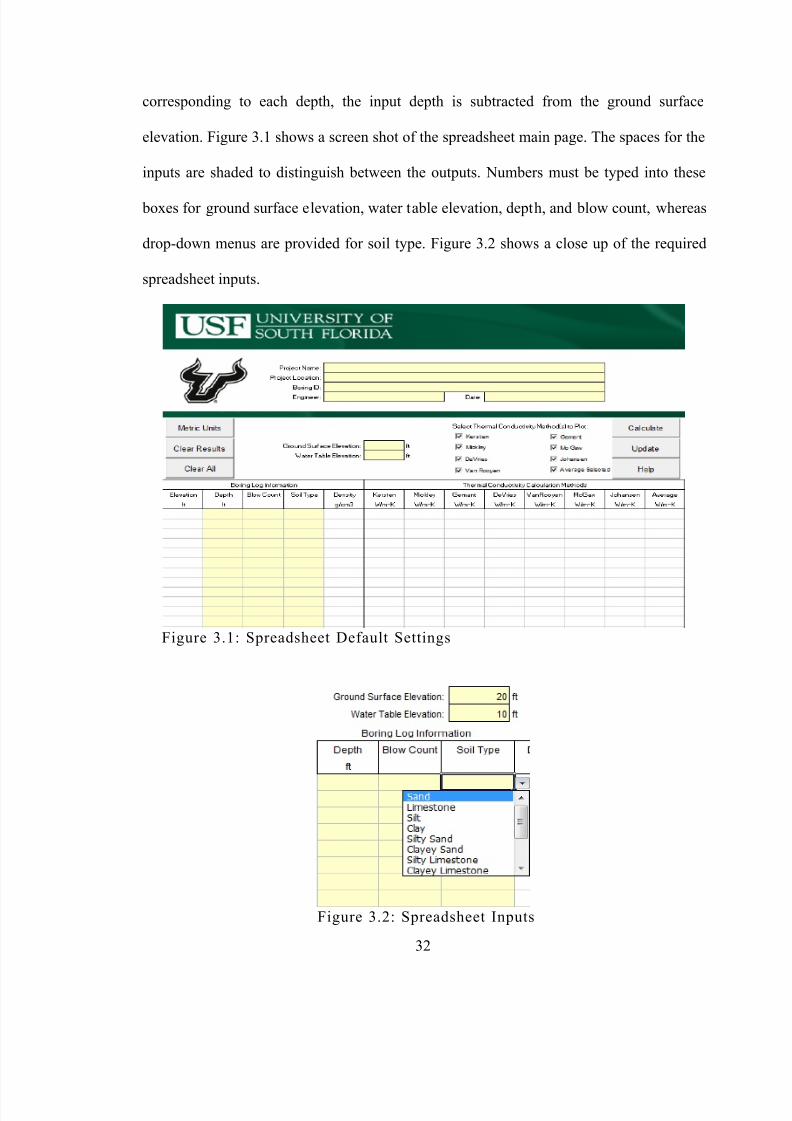
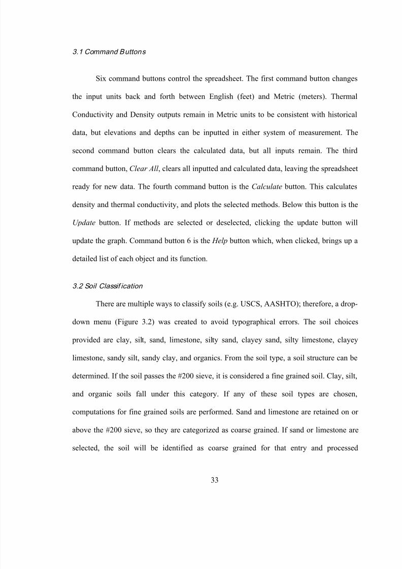
corresponding to each depth, the input depth is subtracted from the ground surface
elevation. Figure 3.1 shows a screen shot of the spreadsheet main page. The spaces for the
inputs are shaded to distinguish between the outputs. Numbers must be typed into these
boxes for ground surface elevation, water table elevation, depth, and blow count, whereas
drop-down menus are provided for soil type. Figure 3.2 shows a close up of the required
spreadsheet inputs.
Figure 3.1: Spreadsheet Default Settings
Figure 3.2: Spreadsheet Inputs
8/16/2019 Thermal Conductivity of Soils From the Analysis of Boring Logs
http://slidepdf.com/reader/full/thermal-conductivity-of-soils-from-the-analysis-of-boring-logs 44/96
33
3.1 Command Buttons
Six command buttons control the spreadsheet. The first command button changes
the input units back and forth between English (feet) and Metric (meters). Thermal
Conductivity and Density outputs remain in Metric units to be consistent with historical
data, but elevations and depths can be inputted in either system of measurement. The
second command button clears the calculated data, but all inputs remain. The third
command button, Clear All , clears all inputted and calculated data, leaving the spreadsheet
ready for new data. The fourth command button is the Calculate button. This calculates
density and thermal conductivity, and plots the selected methods. Below this button is the
Update button. If methods are selected or deselected, clicking the update button will
update the graph. Command button 6 is the Help button which, when clicked, brings up a
detailed list of each object and its function.
3.2 Soil Classif ication
There are multiple ways to classify soils (e.g. USCS, AASHTO); therefore, a drop-
down menu (Figure 3.2) was created to avoid typographical errors. The soil choices
provided are clay, silt, sand, limestone, silty sand, clayey sand, silty limestone, clayey
limestone, sandy silt, sandy clay, and organics. From the soil type, a soil structure can be
determined. If the soil passes the #200 sieve, it is considered a fine grained soil. Clay, silt,
and organic soils fall under this category. If any of these soil types are chosen,
computations for fine grained soils are performed. Sand and limestone are retained on or
above the #200 sieve, so they are categorized as coarse grained. If sand or limestone are
selected, the soil will be identified as coarse grained for that entry and processed
8/16/2019 Thermal Conductivity of Soils From the Analysis of Boring Logs
http://slidepdf.com/reader/full/thermal-conductivity-of-soils-from-the-analysis-of-boring-logs 45/96
34
accordingly. For the soil types consisting of a mix of coarse and fine grained soils, the soil
structure is labeled as “mixed” and computations include raising the thermal conductivity
of both fine and coarse grained soils to their respective volumetric fractions.
3.3 Moi stur e Content
The moisture content of a soil changes with its position relative to the water table.
At the water table and below, it can be assumed that the soil is saturated for most cases.
Above the water table, soil type and distance above the water table must be taken into
account. The University of South Florida performed studies on the changes in moisture
content with relation to the water table for many soil. Three common Florida soils were
chosen from this analysis: one with a high clay content, one with a high silt content, and
one with a high sand content. Limestone was not present in this study, but because it is
typically found below the water table, it can be considered saturated for this application.
Because sand and limestone are coarse grained soils, limestone above the water table is
assumed to have the wicking characteristics of sand. Figures 3.3 through 3.5 show the
changes in moisture content with respect to elevation above the water table for the chosen
clay, silt, and sand. The equations used to calculate thermal conductivity require moisture
contents to be separated into 5%, 10%, 20% and saturated to match available thermal
conductivity correlations. To do this, the graphs were sectioned off and labeled
accordingly.
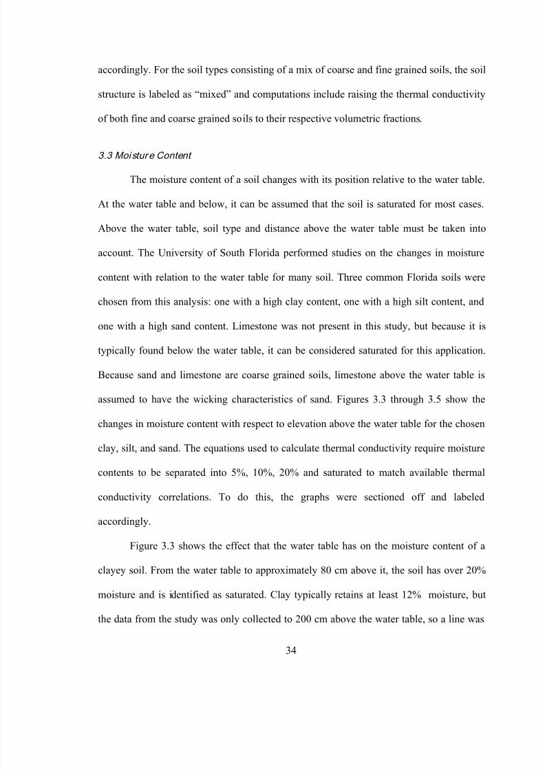
Figure 3.3 shows the effect that the water table has on the moisture content of a
clayey soil. From the water table to approximately 80 cm above it, the soil has over 20%
moisture and is identified as saturated. Clay typically retains at least 12% moisture, but
the data from the study was only collected to 200 cm above the water table, so a line was
8/16/2019 Thermal Conductivity of Soils From the Analysis of Boring Logs
http://slidepdf.com/reader/full/thermal-conductivity-of-soils-from-the-analysis-of-boring-logs 46/96
35
extrapolated, following the same slope, to extend up to a moisture content of 12%. This
point was 780 cm above the water table. Between 80cm and 780 cm, the soil is labeled as
having a moisture content of 20%. Data for 12% moisture is not available; therefore, the
10% moisture content curves are used for clayey soils greater than 780 cm above the water
table.
Figure 3.3: Moisture Content above Water Table for a Clayey Soil
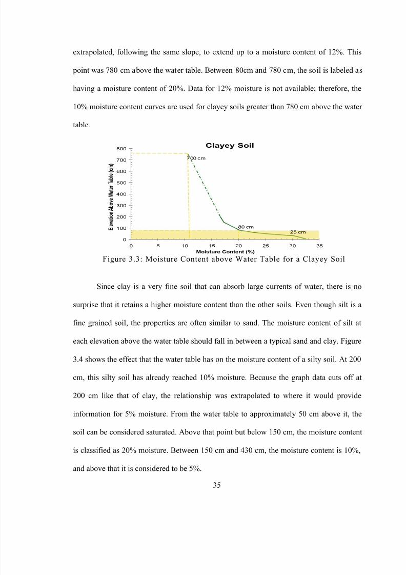
Since clay is a very fine soil that can absorb large currents of water, there is no
surprise that it retains a higher moisture content than the other soils. Even though silt is a
fine grained soil, the properties are often similar to sand. The moisture content of silt at
each elevation above the water table should fall in between a typical sand and clay. Figure
3.4 shows the effect that the water table has on the moisture content of a silty soil. At 200
cm, this silty soil has already reached 10% moisture. Because the graph data cuts off at
200 cm like that of clay, the relationship was extrapolated to where it would provide
information for 5% moisture. From the water table to approximately 50 cm above it, the
soil can be considered saturated. Above that point but below 150 cm, the moisture content
is classified as 20% moisture. Between 150 cm and 430 cm, the moisture content is 10%,
and above that it is considered to be 5%.
0
100
200
300
400
500
600
700
800
0 5 10 15 20 25 30 35
E l e v a t i o n
A b o v e
W a t e r
T a b l e ( c m )
Moisture Content (%)
Clayey Soil
80 cm
700 cm
25 cm
8/16/2019 Thermal Conductivity of Soils From the Analysis of Boring Logs
http://slidepdf.com/reader/full/thermal-conductivity-of-soils-from-the-analysis-of-boring-logs 47/96
36
Figure 3.4: Moisture Content above Water Table for a Silty Soil
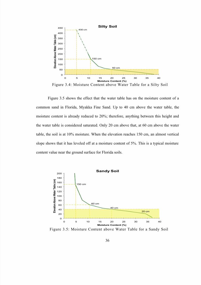
Figure 3.5 shows the effect that the water table has on the moisture content of a
common sand in Florida, Myakka Fine Sand. Up to 40 cm above the water table, the
moisture content is already reduced to 20%; therefore, anything between this height and
the water table is considered saturated. Only 20 cm above that, at 60 cm above the water
table, the soil is at 10% moisture. When the elevation reaches 150 cm, an almost vertical
slope shows that it has leveled off at a moisture content of 5%. This is a typical moisture
content value near the ground surface for Florida soils.
Figure 3.5: Moisture Content above Water Table for a Sandy Soil
0
50
100
150
200
250
300
350
400
450
0 5 10 15 20 25 30 35 40
E l e v a t i o n A b o v e W a t e r T a b l e
( c m )
Moisture Content (%)
Silty Soil
50 cm
150 cm
430 cm
0
20
40
60
80
100
120
140
160
180
200
0 5 10 15 20 25 30 35 40
E l e v a t i o n A b o v e W a t e r T a b l e
( c m )
Moisture Content (%)
Sandy Soil
150 cm
60 cm
40 cm
20 cm
8/16/2019 Thermal Conductivity of Soils From the Analysis of Boring Logs
http://slidepdf.com/reader/full/thermal-conductivity-of-soils-from-the-analysis-of-boring-logs 48/96
37
3.4 Density
The relationships cited in Chapter 2 for thermal conductivity all relate to the
density of the soil as well as the saturation and structure. As a result, making use of
correlations from SPT data to density was a necessary first step. This could also be used to
establish the void ratio and saturation when the soil is not submerged. See Figure 2.16 in
Chapter 2 for the linear correlation between number of blows and the unit weight of clay,
silt, and sand.
A correlation for limestone was detained from a study on cohesionless soil
performed by the University of Florida (University of Florida 2009). Therein, the unitweight varied from 90lb/ft 3 to 130lb/ft 3 for soft to medium/hard limestone. A linear
relationship was assumed where 90 lb/ft 3 represents the density at zero blow counts and
130 lb/ft 3 as the density at 60 blow counts. The line has a slope of 0.667 and a y-intercept
of 90.
The data from Figure 2.16 was reproduced and plotted in Figure 3.6, along with
the values produced for limestone. Trendlines were fitted to the data of each soil type in
order to obtain the equation of each line. The spreadsheet uses the inputted soil type to
select the appropriate equation. It then uses that equation to calculate density, where blow
count is the independent variable (x-value) and density is the dependent value (y-value).
The densities that result from using the equations in Figure 3.6 are in terms of lb/ft 3. The
thermal conductivity calculations require density to be converted to the metric units of
g/cm 3. A conversion factor of 0.016g/cm 3 per 1 lb/ft 3 is automatically applied to each
resulting density in the spreadsheet.
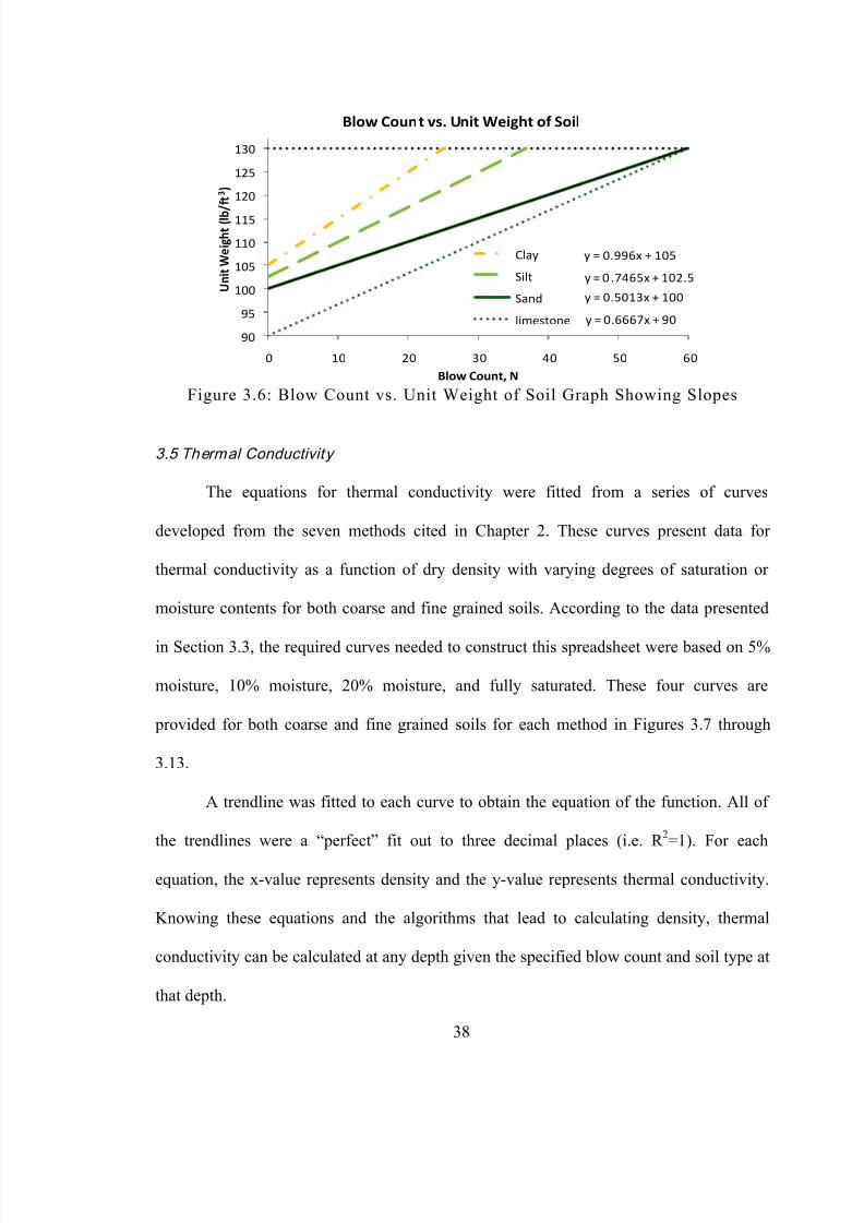
8/16/2019 Thermal Conductivity of Soils From the Analysis of Boring Logs
http://slidepdf.com/reader/full/thermal-conductivity-of-soils-from-the-analysis-of-boring-logs 49/96
38
Figure 3.6: Blow Count vs. Unit Weight of Soil Graph Showing Slopes
3.5 Thermal Conductivity
The equations for thermal conductivity were fitted from a series of curves
developed from the seven methods cited in Chapter 2. These curves present data for
thermal conductivity as a function of dry density with varying degrees of saturation or
moisture contents for both coarse and fine grained soils. According to the data presented
in Section 3.3, the required curves needed to construct this spreadsheet were based on 5%
moisture, 10% moisture, 20% moisture, and fully saturated. These four curves are
provided for both coarse and fine grained soils for each method in Figures 3.7 through
3.13.
A trendline was fitted to each curve to obtain the equation of the function. All of
the trendlines were a “ perfect ” fit out to three decimal places (i.e. R 2=1). For each
equation, the x-value represents density and the y-value represents thermal conductivity.
Knowing these equations and the algorithms that lead to calculating density, thermal
conductivity can be calculated at any depth given the specified blow count and soil type at
that depth.
y = 0.996x + 105
y = 0 .7465x + 102.5
y = 0.5013x + 100
y = 0.6667x + 9090
95
100
105
110
115
120
125
130
0 10 20 30 40 50 60
U n i t W e i g h t ( l b
/ f t 3 )
Blow Count, N
Blow Count vs. Unit Weight of Soil
Clay
Silt
Sand
limestone
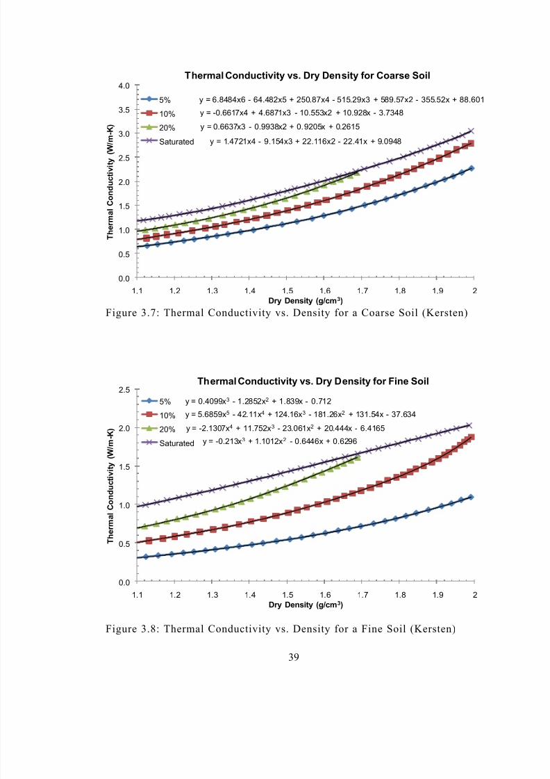
8/16/2019 Thermal Conductivity of Soils From the Analysis of Boring Logs
http://slidepdf.com/reader/full/thermal-conductivity-of-soils-from-the-analysis-of-boring-logs 50/96
39
Figure 3.7: Thermal Conductivity vs. Density for a Coarse Soil (Kersten)
Figure 3.8: Thermal Conductivity vs. Density for a Fine Soil (Kersten)
y = 6.8484x6 - 64.482x5 + 250.87x4 - 515.29x3 + 589.57x2 - 355.52x + 88.601
y = -0.6617x4 + 4.6871x3 - 10.553x2 + 10.928x - 3.7348
y = 0.6637x3 - 0.9938x2 + 0.9205x + 0.2615
y = 1.4721x4 - 9.154x3 + 22.116x2 - 22.41x + 9.0948
0.0
0.5
1.0
1.5
2.0
2.5
3.0
3.5
4.0
1.1 1.2 1.3 1.4 1.5 1.6 1.7 1.8 1.9 2
T h e r m a l
C o n
d u c t i v i t y
( W / m - K
)
Dry Density (g/cm 3)
Thermal Conductivity vs. Dry Density for Coarse Soil
5%
10%
20%
Saturated
y = 0.4099x 3 - 1.2852x 2 + 1.839x - 0.712
y = 5.6859x 5 - 42.11x 4 + 124.16x 3 - 181.26x 2 + 131.54x - 37.634
y = -2.1307x 4 + 11.752x 3 - 23.061x 2 + 20.444x - 6.4165
y = -0.213x 3 + 1.1012x 2 - 0.6446x + 0.6296
0.0
0.5
1.0
1.5
2.0
2.5
1.1 1.2 1.3 1.4 1.5 1.6 1.7 1.8 1.9 2
T h e r m a l
C o n
d u c t i v i t y
( W / m - K
)
Dry Density (g/cm 3)
Thermal Conductivity vs. Dry Density for Fine Soil
5%
10%
20%
Saturated
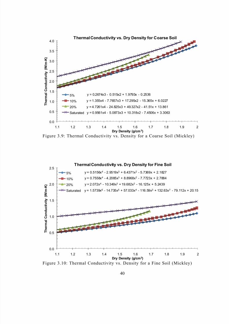
8/16/2019 Thermal Conductivity of Soils From the Analysis of Boring Logs
http://slidepdf.com/reader/full/thermal-conductivity-of-soils-from-the-analysis-of-boring-logs 51/96
40
Figure 3.9: Thermal Conductivity vs. Density for a Coarse Soil (Mickley)
Figure 3.10: Thermal Conductivity vs. Density for a Fine Soil (Mickley)
y = 0.2674x3 - 0.515x2 + 1.9793x - 0.2536
y = 1.355x4 - 7.7657x3 + 17.295x2 - 15.365x + 6.0227
y = 4.7261x4 - 24.825x3 + 49.327x2 - 41.51x + 13.861
y = 0.9561x4 - 5.0873x3 + 10.318x2 - 7.4506x + 3.3063
0.0
0.5
1.0
1.5
2.0
2.5
3.0
3.5
4.0
1.1 1.2 1.3 1.4 1.5 1.6 1.7 1.8 1.9 2
T h e r m a l
C o n d u c t i v i t y
( W / m - K )
Dry Density (g/cm 3)
Thermal Conductivity vs. Dry Density for Coarse Soil
5%
10%
20%
Saturated
y = 0.5156x 4 - 2.9519x 3 + 6.4371x 2 - 5.7369x + 2.1827
y = 0.7558x 4 - 4.2085x 3 + 8.8968x 2 - 7.7723x + 2.7884
y = 2.072x 4 - 10.349x 3 + 19.682x 2 - 16.125x + 5.2439
y = 1.5739x 6 - 14.735x 5 + 57.033x 4 - 116.59x 3 + 132.63x 2 - 79.112x + 20.15
0.0
0.5
1.0
1.5
2.0
2.5
1.1 1.2 1.3 1.4 1.5 1.6 1.7 1.8 1.9 2
T h e r m a l C o n
d u c t i v i t y
( W / m - K
)
Dry Density (g/cm 3)
Thermal Conductivity vs. Dry Density for Fine Soil
5%
10%
20%
Saturated
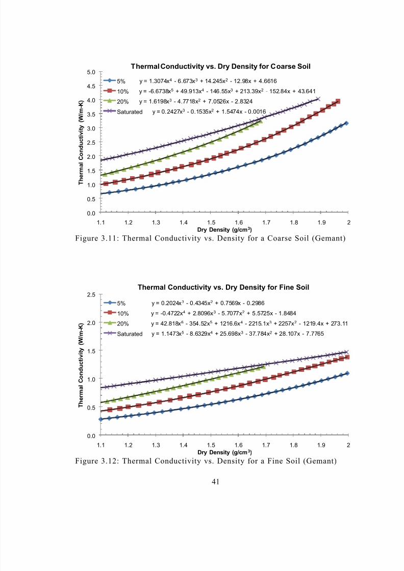
8/16/2019 Thermal Conductivity of Soils From the Analysis of Boring Logs
http://slidepdf.com/reader/full/thermal-conductivity-of-soils-from-the-analysis-of-boring-logs 52/96
41
Figure 3.11: Thermal Conductivity vs. Density for a Coarse Soil (Gemant)
Figure 3.12: Thermal Conductivity vs. Density for a Fine Soil (Gemant)
y = 1.3074x 4 - 6.673x 3 + 14.245x 2 - 12.98x + 4.6616
y = -6.6738x 5 + 49.913x 4 - 146.55x 3 + 213.39x 2 - 152.84x + 43.641
y = 1.6198x 3 - 4.7718x 2 + 7.0526x - 2.8324
y = 0.2427x 3 - 0.1535x 2 + 1.5474x - 0.0016
0.0
0.5
1.0
1.5
2.0
2.5
3.0
3.5
4.0
4.5
5.0
1.1 1.2 1.3 1.4 1.5 1.6 1.7 1.8 1.9 2
T h e r m a l
C o n
d u c t i v i t y
( W / m - K )
Dry Density (g/cm 3)
Thermal Conductivity vs. Dry Density for Coarse Soil
5%
10%
20%
Saturated
y = 0.2024x 3 - 0.4345x 2 + 0.7569x - 0.2986
y = -0.4722x 4 + 2.8096x 3 - 5.7077x 2 + 5.5725x - 1.8484
y = 42.818x 6 - 354.52x 5 + 1216.6x 4 - 2215.1x 3 + 2257x 2 - 1219.4x + 273.11
y = 1.1473x 5 - 8.6329x 4 + 25.698x 3 - 37.784x 2 + 28.107x - 7.7765
0.0
0.5
1.0
1.5
2.0
2.5
1.1 1.2 1.3 1.4 1.5 1.6 1.7 1.8 1.9 2
T h e r m a l
C o n d u c t i v i t y
( W / m - K
)
Dry Density (g/cm 3)
Thermal Conductivity vs. Dry Density for Fine Soil
5%
10%
20%
Saturated
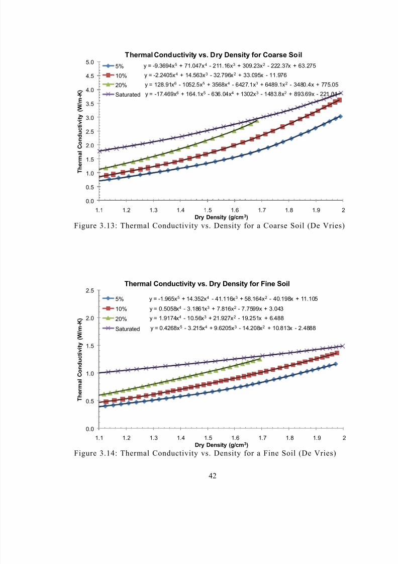
8/16/2019 Thermal Conductivity of Soils From the Analysis of Boring Logs
http://slidepdf.com/reader/full/thermal-conductivity-of-soils-from-the-analysis-of-boring-logs 53/96
42
Figure 3.13: Thermal Conductivity vs. Density for a Coarse Soil (De Vries)
Figure 3.14: Thermal Conductivity vs. Density for a Fine Soil (De Vries)
y = -9.3694x 5 + 71.047x 4 - 211.16x 3 + 309.23x 2 - 222.37x + 63.275
y = -2.2405x 4 + 14.563x 3 - 32.796x 2 + 33.095x - 11.976
y = 128.91x 6 - 1052.5x 5 + 3568x 4 - 6427.1x 3 + 6489.1x 2 - 3480.4x + 775.05
y = -17.469x 6 + 164.1x 5 - 636.04x 4 + 1302x 3 - 1483.8x 2 + 893.69x - 221.01
0.0
0.5
1.0
1.5
2.0
2.5
3.0
3.5
4.0
4.5
5.0
1.1 1.2 1.3 1.4 1.5 1.6 1.7 1.8 1.9 2
T h e r m a l
C o n
d u c t i v i t y
( W / m - K
)
Dry Density (g/cm 3)
Thermal Conductivity vs. Dry Density for Coarse Soil
5%
10%
20%
Saturated
y = -1.965x 5 + 14.352x 4 - 41.116x 3 + 58.164x 2 - 40.198x + 11.105
y = 0.5058x 4 - 3.1861x 3 + 7.816x 2 - 7.7599x + 3.043
y = 1.9174x 4 - 10.56x 3 + 21.927x 2 - 19.251x + 6.488
y = 0.4268x 5 - 3.215x 4 + 9.6205x 3 - 14.208x 2 + 10.813x - 2.4888
0.0
0.5
1.0
1.5
2.0
2.5
1.1 1.2 1.3 1.4 1.5 1.6 1.7 1.8 1.9 2
T h e r m a l
C o n
d u c t i v i t y
( W / m - K
)
Dry Density (g/cm 3)
Thermal Conductivity vs. Dry Density for Fine Soil
5%
10%
20%
Saturated
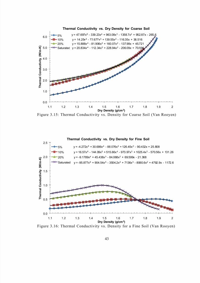
8/16/2019 Thermal Conductivity of Soils From the Analysis of Boring Logs
http://slidepdf.com/reader/full/thermal-conductivity-of-soils-from-the-analysis-of-boring-logs 54/96
43
Figure 3.15: Thermal Conductivity vs. Density for Coarse Soil (Van Rooyen)
Figure 3.16: Thermal Conductivity vs. Density for a Fine Soil (Van Rooyen)
y = 47.697x 5 - 339.23x 4 + 963.08x 3 - 1358.7x 2 + 952.87x - 265.6
y = 14.25x 4 - 72.677x 3 + 139.55x 2 - 116.35x + 36.516y = 15.888x 4 - 81.906x 3 + 160.07x 2 - 137.98x + 45.721y = 20.834x 4 - 112.34x 3 + 228.94x 2 - 206.09x + 70.596
0.0
1.0
2.0
3.0
4.0
5.0
6.0
1.1 1.2 1.3 1.4 1.5 1.6 1.7 1.8 1.9 2
T h e r m a l
C o n
d u c t i v i t y
( W / m - K
)
Dry Density (g/cm 3)
Thermal Conductivity vs. Dry Density for Coarse Soil
5%10%20%
Saturated
y = -4.272x 5 + 30.686x 4 - 88.076x 3 + 126.45x 2 - 90.432x + 25.808
y = 16.57x 6 - 144.09x 5 + 515.66x 4 - 973.97x 3 + 1025.4x 2 - 570.56x + 131.26
y = -9.1789x 4 + 45.438x 3 - 84.068x 2 + 69.599x - 21.368
y = -95.877x 6 + 904.54x 5 - 3504.2x 4 + 7136x 3 - 8060.6x 2 + 4792.9x - 1172.6
0.0
0.5
1.0
1.5
2.0
2.5
1.1 1.2 1.3 1.4 1.5 1.6 1.7 1.8 1.9 2
T h e r m a l
C o n
d u c t i v i t y
( W / m - K
)
Dry Density (g/cm 3)
Thermal Conductivity vs. Dry Density for Fine Soil
5%
10%
20%
Saturated
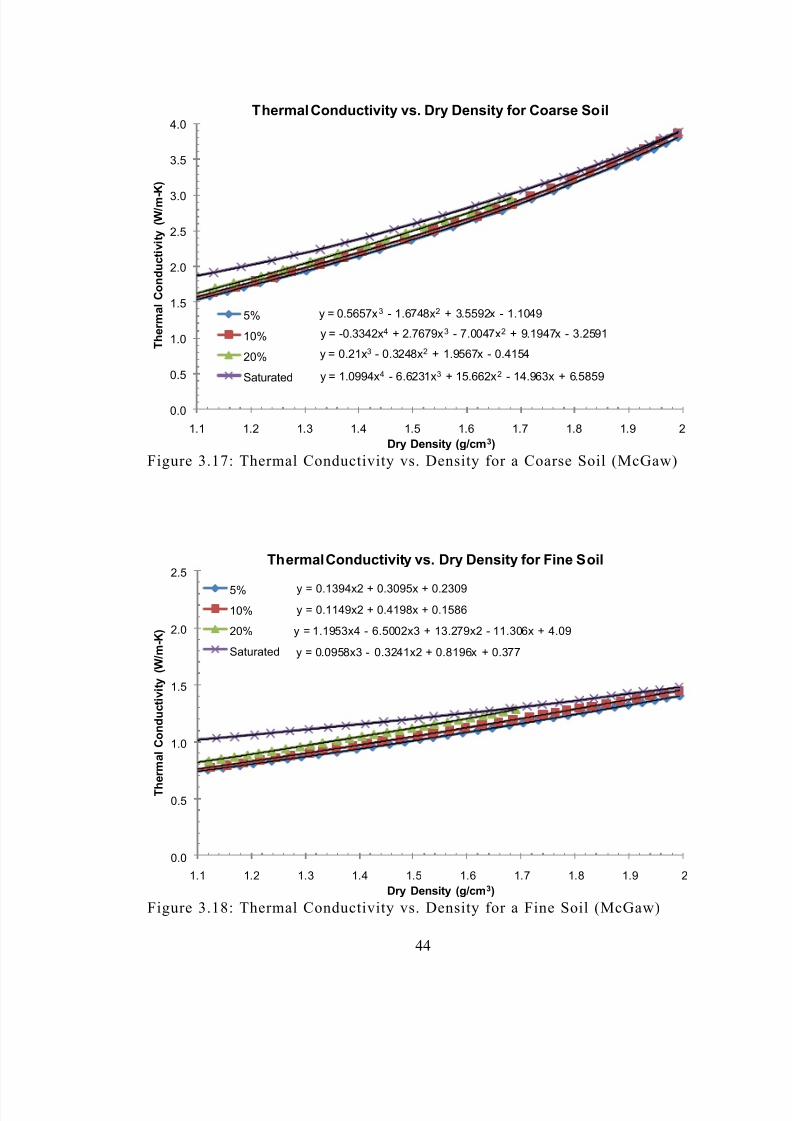
8/16/2019 Thermal Conductivity of Soils From the Analysis of Boring Logs
http://slidepdf.com/reader/full/thermal-conductivity-of-soils-from-the-analysis-of-boring-logs 55/96
44
Figure 3.17: Thermal Conductivity vs. Density for a Coarse Soil (McGaw)
Figure 3.18: Thermal Conductivity vs. Density for a Fine Soil (McGaw)
y = 0.5657x 3 - 1.6748x 2 + 3.5592x - 1.1049
y = -0.3342x 4 + 2.7679x 3 - 7.0047x 2 + 9.1947x - 3.2591
y = 0.21x 3 - 0.3248x 2 + 1.9567x - 0.4154
y = 1.0994x 4 - 6.6231x 3 + 15.662x 2 - 14.963x + 6.5859
0.0
0.5
1.0
1.5
2.0
2.5
3.0
3.5
4.0
1.1 1.2 1.3 1.4 1.5 1.6 1.7 1.8 1.9 2
T h e r m a l
C o n
d u c t i v i t y
( W / m - K )
Dry Density (g/cm 3)
Thermal Conductivity vs. Dry Density for Coarse Soil
5%
10%
20%
Saturated
y = 0.1394x2 + 0.3095x + 0.2309y = 0.1149x2 + 0.4198x + 0.1586
y = 1.1953x4 - 6.5002x3 + 13.279x2 - 11.306x + 4.09
y = 0.0958x3 - 0.3241x2 + 0.8196x + 0.377
0.0
0.5
1.0
1.5
2.0
2.5
1.1 1.2 1.3 1.4 1.5 1.6 1.7 1.8 1.9 2
T h e r m a l C o n d u c t i v i t y
( W / m - K
)
Dry Density (g/cm 3)
Thermal Conductivity vs. Dry Density for Fine Soil
5%10%
20%
Saturated
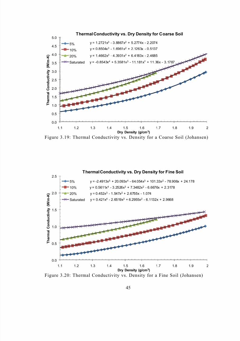
8/16/2019 Thermal Conductivity of Soils From the Analysis of Boring Logs
http://slidepdf.com/reader/full/thermal-conductivity-of-soils-from-the-analysis-of-boring-logs 56/96
45
Figure 3.19: Thermal Conductivity vs. Density for a Coarse Soil (Johansen)
Figure 3.20: Thermal Conductivity vs. Density for a Fine Soil (Johansen)
y = 1.2721x 3 - 3.8867x 2 + 5.2774x - 2.2074
y = 0.8504x 3 - 1.6961x 2 + 2.1263x - 0.5137
y = 1.4662x 3 - 4.3931x 2 + 6.4183x - 2.4685
y = -0.8543x 4 + 5.3581x 3 - 11.181x 2 + 11.36x - 3.1787
0.0
0.5
1.0
1.5
2.0
2.5
3.0
3.5
4.0
4.5
5.0
1.1 1.2 1.3 1.4 1.5 1.6 1.7 1.8 1.9 2
T h e r m a l
C o n d u c t i v i t y
( W / m - K
)
Dry Density (g/cm 3)
Thermal Conductivity vs. Dry Density for Coarse Soil
5%
10%
20%
Saturated
y = -2.4913x 5 + 20.093x 4 - 64.054x 3 + 101.33x 2 - 78.906x + 24.178
y = 0.5611x 4 - 3.2526x 3 + 7.3482x 2 - 6.6676x + 2.3178
y = 0.452x 3 - 1.547x 2 + 2.6755x - 1.074
y = 0.421x 4 - 2.6519x 3 + 6.2955x 2 - 6.1132x + 2.9668
0.0
0.5
1.0
1.5
2.0
2.5
1.1 1.2 1.3 1.4 1.5 1.6 1.7 1.8 1.9 2
T h e r m a l
C o n
d u c t i v i t y
( W / m - K
)
Dry Density (g/cm 3)
Thermal Conductivity vs. Dry Density for Fine Soil
5%
10%
20%
Saturated
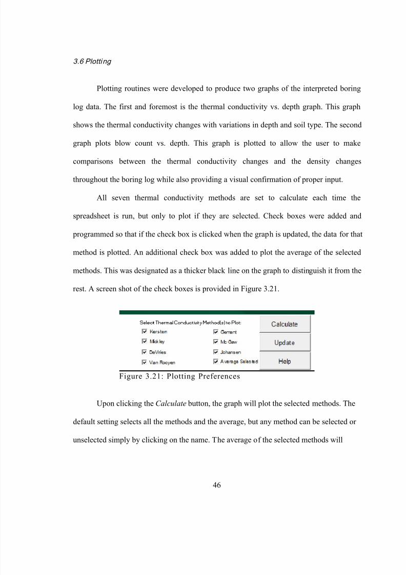
8/16/2019 Thermal Conductivity of Soils From the Analysis of Boring Logs
http://slidepdf.com/reader/full/thermal-conductivity-of-soils-from-the-analysis-of-boring-logs 57/96
46
3.6 Plotti ng
Plotting routines were developed to produce two graphs of the interpreted boring
log data. The first and foremost is the thermal conductivity vs. depth graph. This graph
shows the thermal conductivity changes with variations in depth and soil type. The second
graph plots blow count vs. depth. This graph is plotted to allow the user to make
comparisons between the thermal conductivity changes and the density changes
throughout the boring log while also providing a visual confirmation of proper input.
All seven thermal conductivity methods are set to calculate each time thespreadsheet is run, but only to plot if they are selected. Check boxes were added and
programmed so that if the check box is clicked when the graph is updated, the data for that
method is plotted. An additional check box was added to plot the average of the selected
methods. This was designated as a thicker black line on the graph to distinguish it from the
rest. A screen shot of the check boxes is provided in Figure 3.21.
Figure 3.21: Plotting Preferences
Upon clicking the Calculate button, the graph will plot the selected methods. The
default setting selects all the methods and the average, but any method can be selected or
unselected simply by clicking on the name. The average of the selected methods will
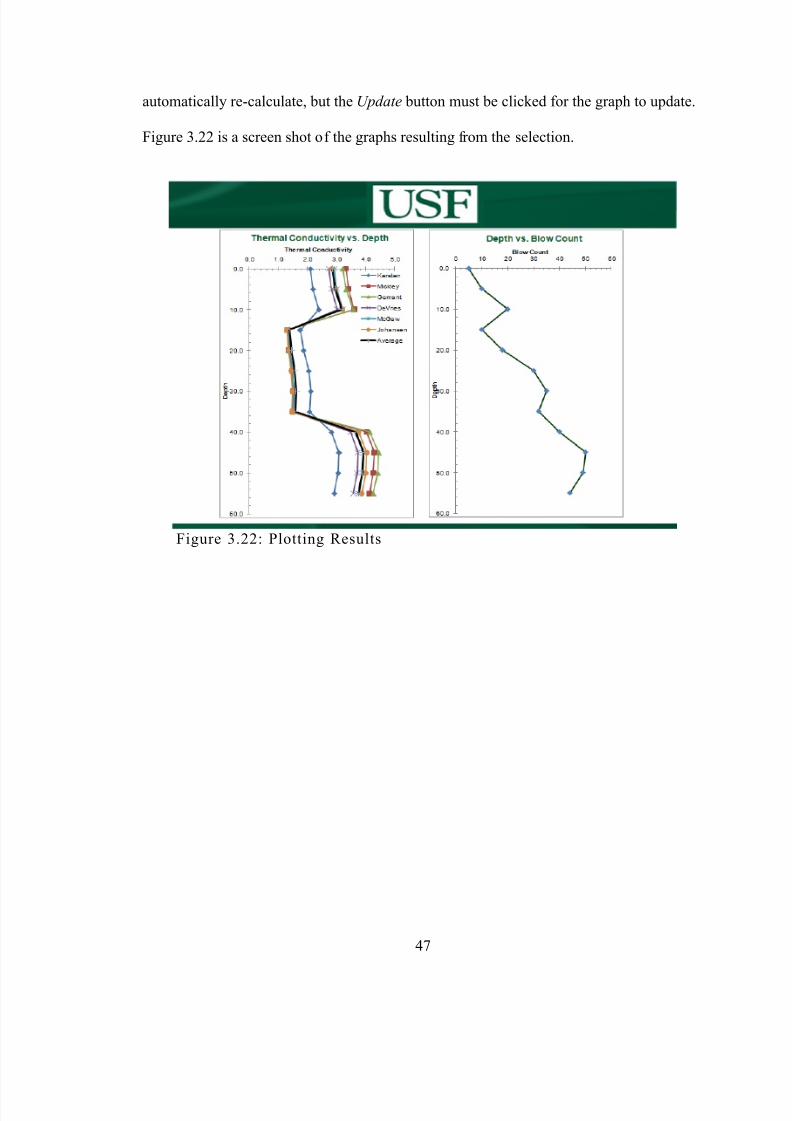
8/16/2019 Thermal Conductivity of Soils From the Analysis of Boring Logs
http://slidepdf.com/reader/full/thermal-conductivity-of-soils-from-the-analysis-of-boring-logs 58/96
47
automatically re-calculate, but the Update button must be clicked for the graph to update.
Figure 3.22 is a screen shot of the graphs resulting from the selection.
Figure 3.22: Plotting Results
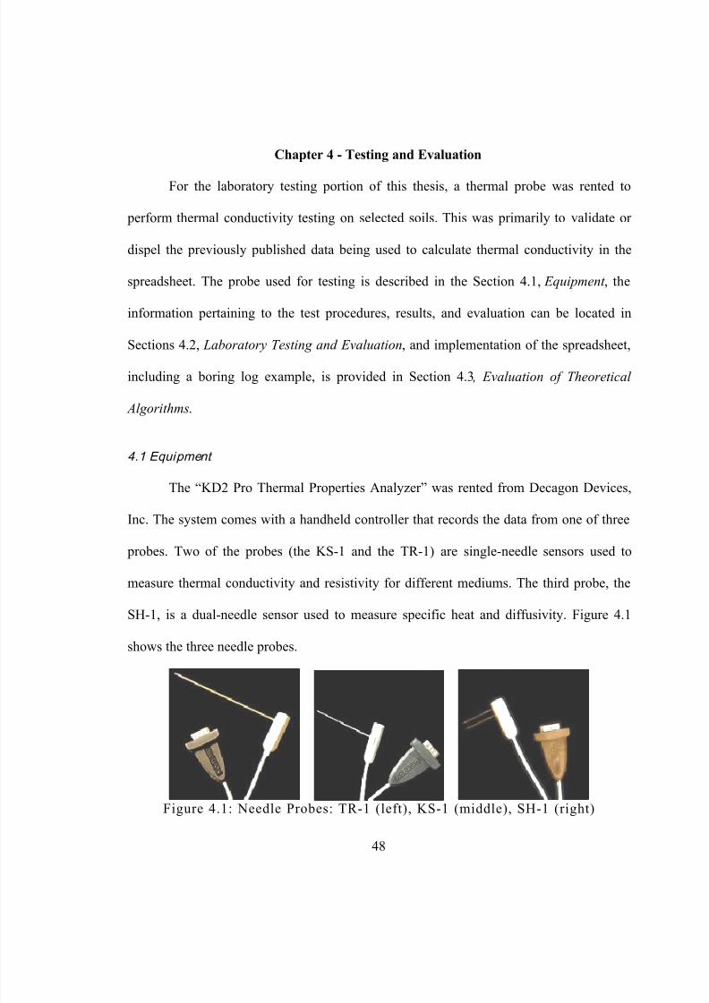
8/16/2019 Thermal Conductivity of Soils From the Analysis of Boring Logs
http://slidepdf.com/reader/full/thermal-conductivity-of-soils-from-the-analysis-of-boring-logs 59/96
48
Chapter 4 - Testing and Evaluation
For the laboratory testing portion of this thesis, a thermal probe was rented to
perform thermal conductivity testing on selected soils. This was primarily to validate or
dispel the previously published data being used to calculate thermal conductivity in the
spreadsheet. The probe used for testing is described in the Section 4.1, Equipment , the
information pertaining to the test procedures, results, and evaluation can be located in
Sections 4.2, Laboratory Testing and Evaluation , and implementation of the spreadsheet,including a boring log example, is provided in Section 4.3 , Evaluation of Theoretical
Algorithms .
4.1 Equipment
The “KD2 Pro Thermal Properties Analyzer” was rented from Decagon Devices,
Inc. The system comes with a handheld controller that records the data from one of three
probes. Two of the probes (the KS-1 and the TR-1) are single-needle sensors used to
measure thermal conductivity and resistivity for different mediums. The third probe, the
SH-1, is a dual-needle sensor used to measure specific heat and diffusivity. Figure 4.1
shows the three needle probes.
Figure 4.1: Needle Probes: TR-1 (left), KS-1 (middle), SH-1 (right)
8/16/2019 Thermal Conductivity of Soils From the Analysis of Boring Logs
http://slidepdf.com/reader/full/thermal-conductivity-of-soils-from-the-analysis-of-boring-logs 60/96
49
The KS-1 is a 60 mm long needle with a 1.3 mm diameter and its thermal
conductivity range is from 0.02 W/m-K to 2.0 W/m-K with ± 5% accuracy. The TR-1 is
the larger of the two single-needle probes. It is a 100 mm long needle with a 2.4 mm
diameter. For thermal conductivity, its range is from 0.10 W/m-K to 4.00 W/m-K with an
accuracy of ± 10%. The SH-1 is the dual-needle probe that consists of two 30 mm long
needles with 1.3 mm diameters, spaced 6 mm apart.
The KS-1 probe applies a smaller amount of heat for a shorter period of time than
the TR-1 probe, making it more suitable for liquids and insulating materials. The dual-
needle probe, SH-1, is primarily designed to read specific heat and diffusivity so this probe was not used for thermal conductivity testing. The TR-1 probe is designed for use in
soil, concrete, rock, and other granular materials. Because of this, the TR-1 probe was
chosen for all thermal conductivity testing.
Testing times for the TR-1 vary between 5 and 10 minutes. Heat is applied for the
first half of the test and readings are taken every 5 or 10 seconds, depending on the chosen
read time. A total of 60 measurements are taken during each test. The longer read time is
suggested for dry granular materials, large grains, or solid samples. A minimum of 2.7
mm of the tested material must surround the probe in all directions to avoid errors while
testing. The KD-2 system follows the specifications outlined in ASTM D5334-08.
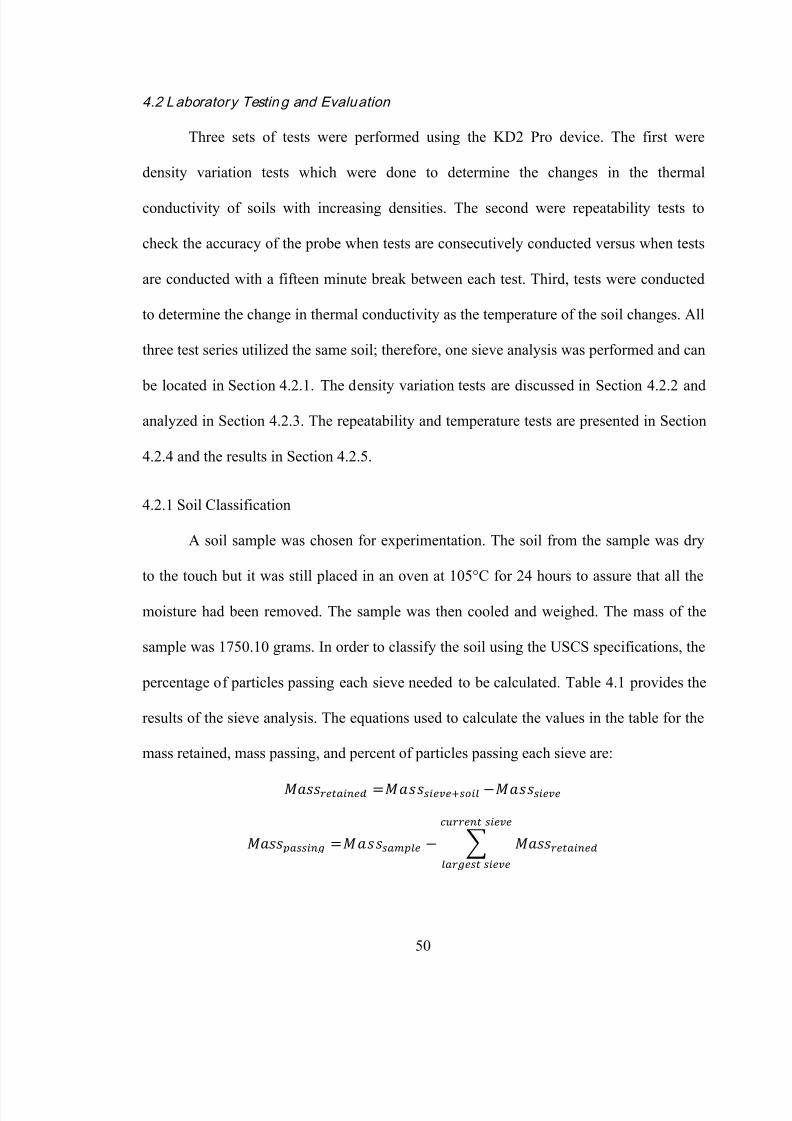
8/16/2019 Thermal Conductivity of Soils From the Analysis of Boring Logs
http://slidepdf.com/reader/full/thermal-conductivity-of-soils-from-the-analysis-of-boring-logs 61/96
50
4.2 L aboratory Testin g and Evalu ation
Three sets of tests were performed using the KD2 Pro device. The first were
density variation tests which were done to determine the changes in the thermal
conductivity of soils with increasing densities. The second were repeatability tests to
check the accuracy of the probe when tests are consecutively conducted versus when tests
are conducted with a fifteen minute break between each test. Third, tests were conducted
to determine the change in thermal conductivity as the temperature of the soil changes. All
three test series utilized the same soil; therefore, one sieve analysis was performed and can
be located in Section 4.2.1. The density variation tests are discussed in Section 4.2.2 andanalyzed in Section 4.2.3. The repeatability and temperature tests are presented in Section
4.2.4 and the results in Section 4.2.5.
4.2.1 Soil Classification
A soil sample was chosen for experimentation. The soil from the sample was dry
to the touch but it was still placed in an oven at 105°C for 24 hours to assure that all the
moisture had been removed. The sample was then cooled and weighed. The mass of the
sample was 1750.10 grams. In order to classify the soil using the USCS specifications, the
percentage of particles passing each sieve needed to be calculated. Table 4.1 provides the
results of the sieve analysis. The equations used to calculate the values in the table for the
mass retained, mass passing, and percent of particles passing each sieve are:
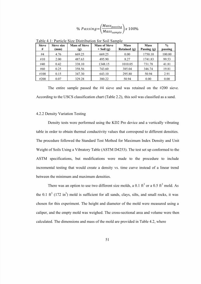
8/16/2019 Thermal Conductivity of Soils From the Analysis of Boring Logs
http://slidepdf.com/reader/full/thermal-conductivity-of-soils-from-the-analysis-of-boring-logs 62/96
51
Table 4.1: Particle Size Distribution for Soil SampleSieve
#
Sieve size
(mm)
Mass of Sieve
(g)
Mass of Sieve
+ Soil (g)
Mass
Retained (g)
Mass
Passing (g)
%
passing#4 4.76 669.25 669.25 0.00 1750.10 100.00
#10 2.00 487.63 495.90 8.27 1741.83 99.53
#40 0.42 338.10 1348.15 1010.05 731.78 41.81#60 0.25 358.56 743.60 385.04 346.74 19.81
#100 0.15 347.30 643.10 295.80 50.94 2.91
#200 0.07 329.28 380.22 50.94 0.00 0.00
The entire sample passed the #4 sieve and was retained on the #200 sieve.
According to the USCS classification chart (Table 2.2), this soil was classified as a sand.
4.2.2 Density Variation Testing
Density tests were performed using the KD2 Pro device and a vertically vibrating
table in order to obtain thermal conductivity values that correspond to different densities.
The procedure followed the Standard Test Method for Maximum Index Density and Unit
Weight of Soils Using a Vibratory Table (ASTM D4253). The test set up conformed to the
ASTM specifications, but modifications were made to the procedure to include
incremental testing that would create a density vs. time curve instead of a linear trend
between the minimum and maximum densities.
There was an option to use two different size molds, a 0.1 ft 3 or a 0.5 ft 3 mold. As
the 0.1 ft 3 (172 in 3) mold is sufficient for all sands, clays, silts, and small rocks, it was
chosen for this experiment. The height and diameter of the mold were measured using a
caliper, and the empty mold was weighed. The cross-sectional area and volume were then
calculated. The dimensions and mass of the mold are provided in Table 4.2, where

8/16/2019 Thermal Conductivity of Soils From the Analysis of Boring Logs
http://slidepdf.com/reader/full/thermal-conductivity-of-soils-from-the-analysis-of-boring-logs 63/96
52
and,
Table 4.2: Mold DimensionsMold Dimensions
Height of Mold 6.12 In
Diameter of Mold 6.00 In
X-sectional Area of Mold 28.27 in 2
Volume of Mold (in3) 172.93 in 3
Volume of Mold (cm3) 2833.75 cm 3
Mass of Mold 3742.80 kg
For the dry tests, a scoop was used to gently place soil in the mold while keeping
the soil as loosely packed as possible. Once the mold was filled, a leveling tool was used
to create an even surface across the top of the mold. The mold with the soil was weighed,
and the weight of the mold was subtracted in order to calculate the mass of dry soil.
The mold was then attached to the vibrating table (Figure 4.2). A minor amount of
settling occurred while in transit, but the change in volume was negligible. To determine
the thermal conductivity for the soil at its loosest state in the mold, the probe was inserted
near the center of the soil sample and a 10 minute test was performed (Figure 4.3). Upon
finishing the test, the probe was removed and the mold was tapped along the sides several
times to allow the soil to settle enough to place the surcharge base plate uniformly on top
of it (Figure 4.4). Once the base plate was applied, the guide sleeve was attached to the top
of the mold. The surcharge weight was lowered through the sleeve and placed on top of
the base plate (Figure 4.5). The complete assembled apparatus is displayed in Figure 4.6.
Using a caliper, the distance from the top of the weight to the top of the sleeve was
measured in two places 180° across from each other (Figure 4.7).
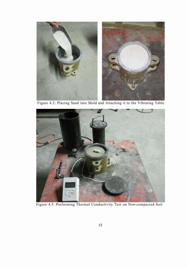
8/16/2019 Thermal Conductivity of Soils From the Analysis of Boring Logs
http://slidepdf.com/reader/full/thermal-conductivity-of-soils-from-the-analysis-of-boring-logs 64/96
53
Figure 4.2: Placing Sand into Mold and Attaching it to the Vibrating Table
Figure 4.3: Performing Thermal Conductivity Test on Non-compacted Soil
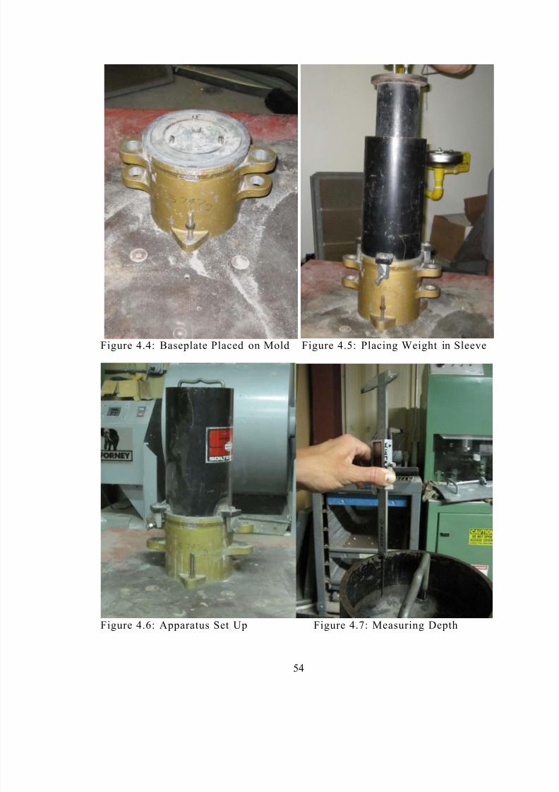
8/16/2019 Thermal Conductivity of Soils From the Analysis of Boring Logs
http://slidepdf.com/reader/full/thermal-conductivity-of-soils-from-the-analysis-of-boring-logs 65/96
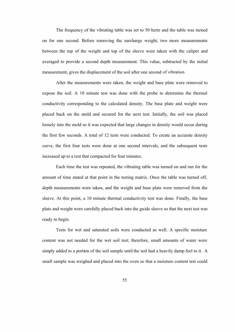
8/16/2019 Thermal Conductivity of Soils From the Analysis of Boring Logs
http://slidepdf.com/reader/full/thermal-conductivity-of-soils-from-the-analysis-of-boring-logs 66/96
55
The frequency of the vibrating table was set to 50 hertz and the table was turned
on for one second. Before removing the surcharge weight, two more measurements
between the top of the weight and top of the sleeve were taken with the caliper and
averaged to provide a second depth measurement. This value, subtracted by the initial
measurement, gives the displacement of the soil after one second of vibration.
After the measurements were taken, the weight and base plate were removed to
expose the soil. A 10 minute test was done with the probe to determine the thermal
conductivity corresponding to the calculated density. The base plate and weight were
placed back on the mold and secured for the next test. Initially, the soil was placedloosely into the mold so it was expected that large changes in density would occur during
the first few seconds. A total of 12 tests were conducted. To create an accurate density
curve, the first four tests were done at one second intervals, and the subsequent tests
increased up to a test that compacted for four minutes.
Each time the test was repeated, the vibrating table was turned on and run for the
amount of time stated at that point in the testing matrix. Once the table was turned off,
depth measurements were taken, and the weight and base plate were removed from the
sleeve. At this point, a 10 minute thermal conductivity test was done. Finally, the base
plate and weight were carefully placed back into the guide sleeve so that the next test was
ready to begin.
Tests for wet and saturated soils were conducted as well. A specific moisture
content was not needed for the wet soil test; therefore, small amounts of water were
simply added to a portion of the soil sample until the soil had a heavily damp feel to it. A
small sample was weighed and placed into the oven so that a moisture content test could
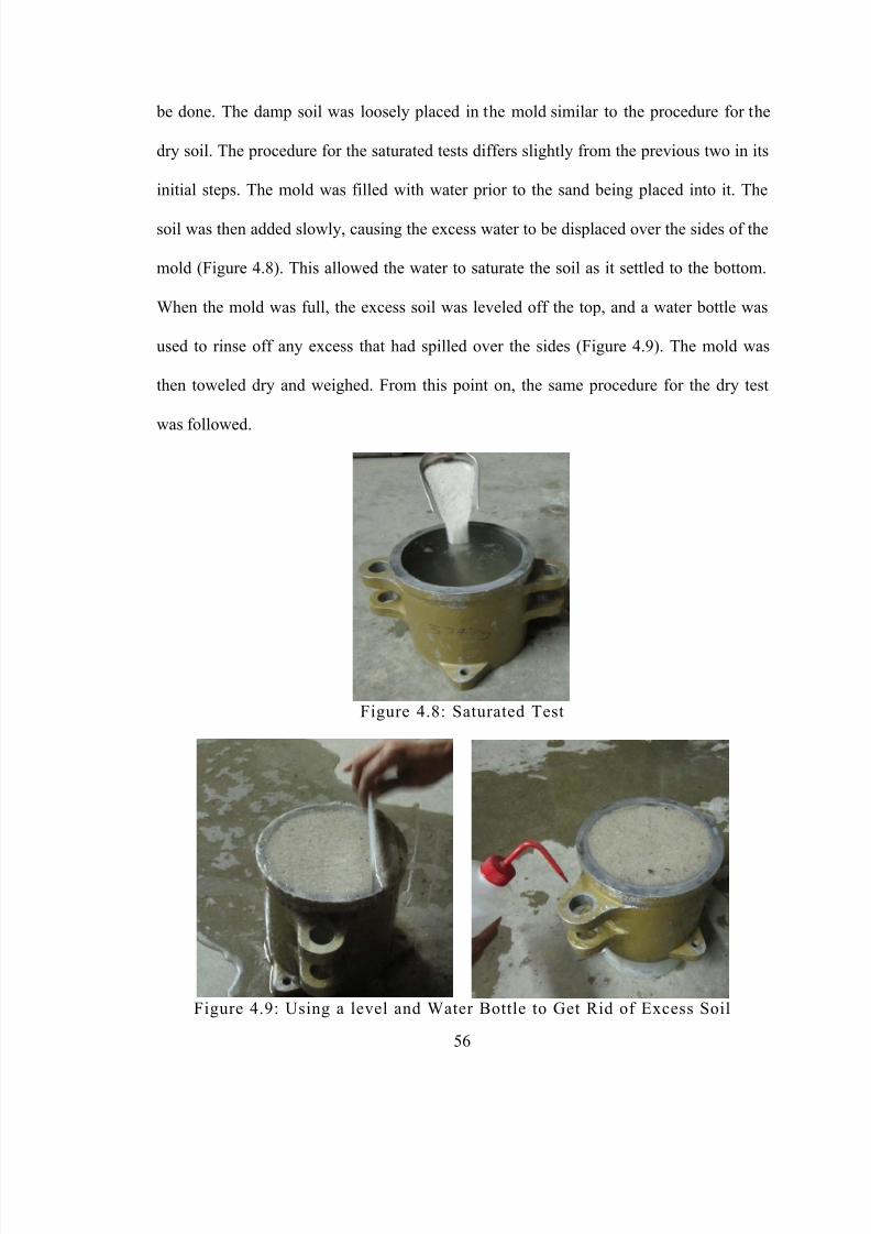
8/16/2019 Thermal Conductivity of Soils From the Analysis of Boring Logs
http://slidepdf.com/reader/full/thermal-conductivity-of-soils-from-the-analysis-of-boring-logs 67/96
56
be done. The damp soil was loosely placed in the mold similar to the procedure for the
dry soil. The procedure for the saturated tests differs slightly from the previous two in its
initial steps. The mold was filled with water prior to the sand being placed into it. The
soil was then added slowly, causing the excess water to be displaced over the sides of the
mold (Figure 4.8). This allowed the water to saturate the soil as it settled to the bottom.
When the mold was full, the excess soil was leveled off the top, and a water bottle was
used to rinse off any excess that had spilled over the sides (Figure 4.9). The mold was
then toweled dry and weighed. From this point on, the same procedure for the dry test
was followed.
Figure 4.8: Saturated Test
Figure 4.9: Using a level and Water Bottle to Get Rid of Excess Soil
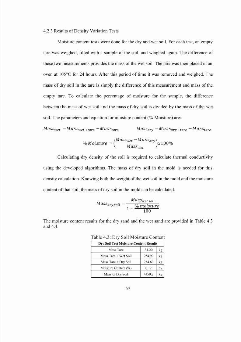
8/16/2019 Thermal Conductivity of Soils From the Analysis of Boring Logs
http://slidepdf.com/reader/full/thermal-conductivity-of-soils-from-the-analysis-of-boring-logs 68/96
57
4.2.3 Results of Density Variation Tests
Moisture content tests were done for the dry and wet soil. For each test, an empty
tare was weighed, filled with a sample of the soil, and weighed again. The difference of
these two measurements provides the mass of the wet soil. The tare was then placed in an
oven at 105°C for 24 hours. After this period of time it was removed and weighed. The
mass of dry soil in the tare is simply the difference of this measurement and mass of the
empty tare. To calculate the percentage of moisture for the sample, the difference
between the mass of wet soil and the mass of dry soil is divided by the mass of the wet
soil. The parameters and equation for moisture content (% Moisture) are:
Calculating dry density of the soil is required to calculate thermal conductivity
using the developed algorithms. The mass of dry soil in the mold is needed for this
density calculation. Knowing both the weight of the wet soil in the mold and the moisture
content of that soil, the mass of dry soil in the mold can be calculated.
The moisture content results for the dry sand and the wet sand are provided in Table 4.3and 4.4.
Table 4.3: Dry Soil Moisture ContentDry Soil Test Moisture Content Results
Mass Tare 31.20 kg
Mass Tare + Wet Soil 254.90 kg
Mass Tare + Dry Soil 254.60 kg
Moisture Content (%) 0.12 %
Mass of Dry Soil 4459.2 kg
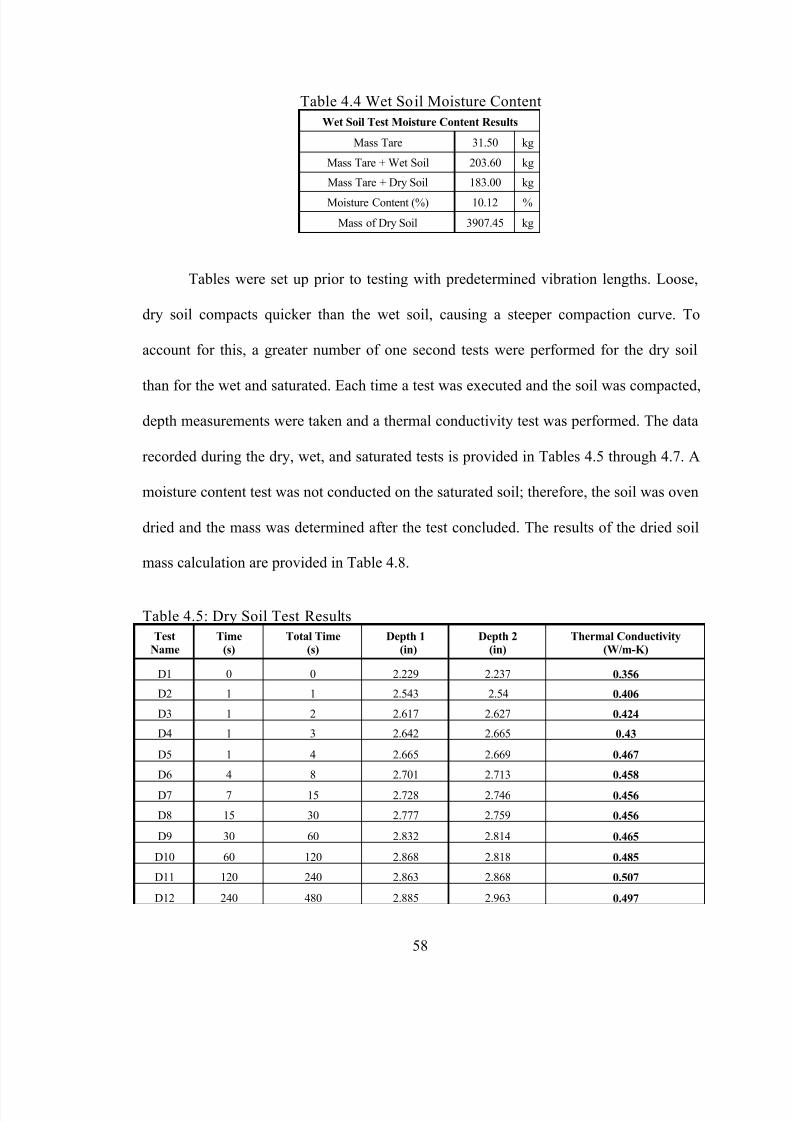
8/16/2019 Thermal Conductivity of Soils From the Analysis of Boring Logs
http://slidepdf.com/reader/full/thermal-conductivity-of-soils-from-the-analysis-of-boring-logs 69/96
58
Table 4.4 Wet Soil Moisture ContentWet Soil Test Moisture Content Results
Mass Tare 31.50 kg
Mass Tare + Wet Soil 203.60 kg
Mass Tare + Dry Soil 183.00 kg
Moisture Content (%) 10.12 %
Mass of Dry Soil 3907.45 kg
Tables were set up prior to testing with predetermined vibration lengths. Loose,
dry soil compacts quicker than the wet soil, causing a steeper compaction curve. To
account for this, a greater number of one second tests were performed for the dry soil
than for the wet and saturated. Each time a test was executed and the soil was compacted,depth measurements were taken and a thermal conductivity test was performed. The data
recorded during the dry, wet, and saturated tests is provided in Tables 4.5 through 4.7. A
moisture content test was not conducted on the saturated soil; therefore, the soil was oven
dried and the mass was determined after the test concluded. The results of the dried soil
mass calculation are provided in Table 4.8.
Table 4.5: Dry Soil Test ResultsTest
NameTime
(s)Total Time
(s)Depth 1
(in)Depth 2
(in)Thermal Conductivity
(W/m-K)
D1 0 0 2.229 2.237 0.356
D2 1 1 2.543 2.54 0.406
D3 1 2 2.617 2.627 0.424
D4 1 3 2.642 2.665 0.43
D5 1 4 2.665 2.669 0.467
D6 4 8 2.701 2.713 0.458
D7 7 15 2.728 2.746 0.456
D8 15 30 2.777 2.759 0.456
D9 30 60 2.832 2.814 0.465
D10 60 120 2.868 2.818 0.485
D11 120 240 2.863 2.868 0.507
D12 240 480 2.885 2.963 0.497
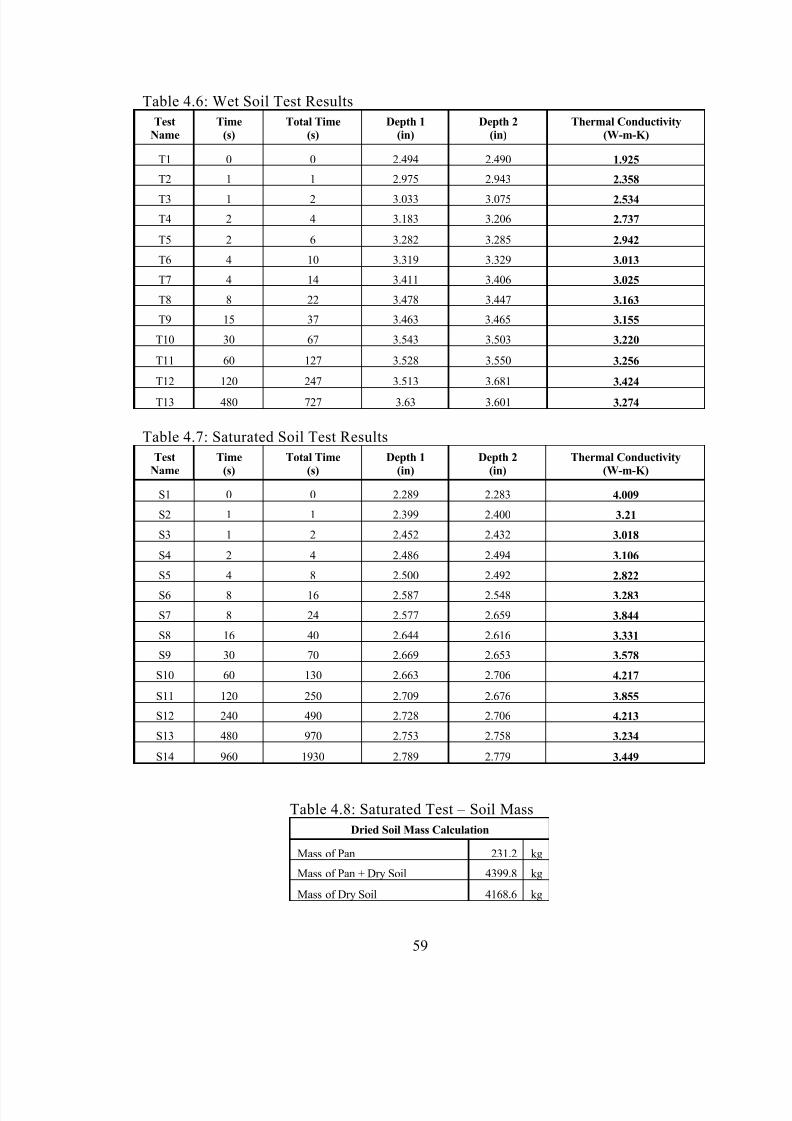
8/16/2019 Thermal Conductivity of Soils From the Analysis of Boring Logs
http://slidepdf.com/reader/full/thermal-conductivity-of-soils-from-the-analysis-of-boring-logs 70/96
59
Table 4.6: Wet Soil Test ResultsTest
NameTime
(s)Total Time
(s)Depth 1
(in)Depth 2
(in)Thermal Conductivity
(W-m-K)
T1 0 0 2.494 2.490 1.925
T2 1 1 2.975 2.943 2.358
T3 1 2 3.033 3.075 2.534
T4 2 4 3.183 3.206 2.737
T5 2 6 3.282 3.285 2.942
T6 4 10 3.319 3.329 3.013
T7 4 14 3.411 3.406 3.025
T8 8 22 3.478 3.447 3.163
T9 15 37 3.463 3.465 3.155
T10 30 67 3.543 3.503 3.220
T11 60 127 3.528 3.550 3.256
T12 120 247 3.513 3.681 3.424
T13 480 727 3.63 3.601 3.274
Table 4.7: Saturated Soil Test ResultsTest
NameTime
(s)Total Time
(s)Depth 1
(in)Depth 2
(in)Thermal Conductivity
(W-m-K)
S1 0 0 2.289 2.283 4.009
S2 1 1 2.399 2.400 3.21
S3 1 2 2.452 2.432 3.018
S4 2 4 2.486 2.494 3.106
S5 4 8 2.500 2.492 2.822
S6 8 16 2.587 2.548 3.283
S7 8 24 2.577 2.659 3.844
S8 16 40 2.644 2.616 3.331
S9 30 70 2.669 2.653 3.578
S10 60 130 2.663 2.706 4.217
S11 120 250 2.709 2.676 3.855
S12 240 490 2.728 2.706 4.213
S13 480 970 2.753 2.758 3.234
S14 960 1930 2.789 2.779 3.449
Table 4.8: Saturated Test – Soil MassDried Soil Mass Calculation
Mass of Pan 231.2 kg
Mass of Pan + Dry Soil 4399.8 kg
Mass of Dry Soil 4168.6 kg
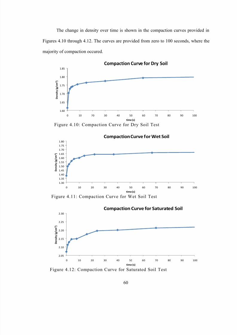
8/16/2019 Thermal Conductivity of Soils From the Analysis of Boring Logs
http://slidepdf.com/reader/full/thermal-conductivity-of-soils-from-the-analysis-of-boring-logs 71/96
60
The change in density over time is shown in the compaction curves provided in
Figures 4.10 through 4.12. The curves are provided from zero to 100 seconds, where the
majority of compaction occured.
Figure 4.10: Compaction Curve for Dry Soil Test
Figure 4.11: Compaction Curve for Wet Soil Test
Figure 4.12: Compaction Curve for Saturated Soil Test
1.60
1.65
1.70
1.75
1.80
1.85
0 10 20 30 40 50 60 70 80 90 100
D e n s i t y
( g / c m 3 )
time (s)
Compaction Curve for Dry Soil
1.30
1.35
1.40
1.45
1.50
1.55
1.60
1.65
1.70
1.75
1.80
0 10 20 30 40 50 60 70 80 90 100
D e n s i t y
( g / c m 3 )
time (s)
Compaction Curve for Wet Soil
2.05
2.10
2.15
2.20
2.25
2.30
0 10 20 30 40 50 60 70 80 90 100
D e n s i t y
( g / c m 3 )
time (s)
Compaction Curve for Saturated Soil

8/16/2019 Thermal Conductivity of Soils From the Analysis of Boring Logs
http://slidepdf.com/reader/full/thermal-conductivity-of-soils-from-the-analysis-of-boring-logs 72/96
61
The two depth measurements from the recorded data were averaged to account for
uneven settling. To calculate the displacement of the soil from compaction, the initial
average depth was subtracted from the average depth of the weight for each measurement
taken. The average depth and soil displacement equations are:
The height of the soil is simply the difference between the height of the mold and
the soil displacement. Volume of the soil can then be calculated by multiplying the soil
height by the cross-sectional area. The spreadsheet requires volume in SI units so this
value was multiplied by the necessary conversion factor to get the result in cm 3. The
equations used to calculate the height and volume of the soil in the mold each time
compaction occurred are
From the results of the moisture content test and the dried soil mass calculation,
the mass of the dry soil was calculated. For the initial, non-compacted test, the volume of
the soil was equivalent to the volume of the mold. Otherwise, the volume of the soil was
calculated from the measured soil displacements. Mass of the dry soil and volume of the
soil are the two parameters required to calculate dry density.
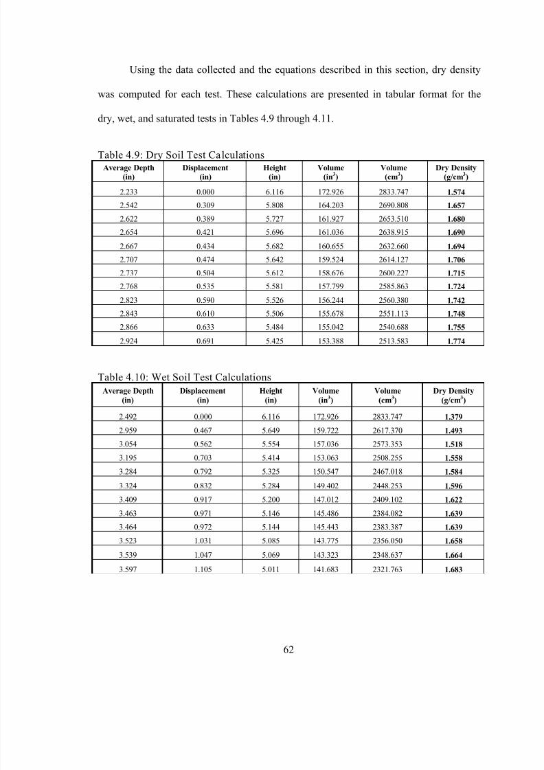
8/16/2019 Thermal Conductivity of Soils From the Analysis of Boring Logs
http://slidepdf.com/reader/full/thermal-conductivity-of-soils-from-the-analysis-of-boring-logs 73/96
62
Using the data collected and the equations described in this section, dry density
was computed for each test. These calculations are presented in tabular format for the
dry, wet, and saturated tests in Tables 4.9 through 4.11.
Table 4.9: Dry Soil Test CalculationsAverage Depth
(in)Displacement
(in)Height
(in)Volume
(in 3)Volume
(cm 3)Dry Density
(g/cm 3)
2.233 0.000 6.116 172.926 2833.747 1.574
2.542 0.309 5.808 164.203 2690.808 1.657
2.622 0.389 5.727 161.927 2653.510 1.680
2.654 0.421 5.696 161.036 2638.915 1.690
2.667 0.434 5.682 160.655 2632.660 1.694
2.707 0.474 5.642 159.524 2614.127 1.706
2.737 0.504 5.612 158.676 2600.227 1.715
2.768 0.535 5.581 157.799 2585.863 1.724
2.823 0.590 5.526 156.244 2560.380 1.742
2.843 0.610 5.506 155.678 2551.113 1.748
2.866 0.633 5.484 155.042 2540.688 1.755
2.924 0.691 5.425 153.388 2513.583 1.774
Table 4.10: Wet Soil Test CalculationsAverage Depth
(in)Displacement
(in)Height
(in)Volume
(in 3)Volume
(cm 3)Dry Density
(g/cm 3)
2.492 0.000 6.116 172.926 2833.747 1.379
2.959 0.467 5.649 159.722 2617.370 1.493
3.054 0.562 5.554 157.036 2573.353 1.518
3.195 0.703 5.414 153.063 2508.255 1.558
3.284 0.792 5.325 150.547 2467.018 1.584
3.324 0.832 5.284 149.402 2448.253 1.596
3.409 0.917 5.200 147.012 2409.102 1.622
3.463 0.971 5.146 145.486 2384.082 1.639
3.464 0.972 5.144 145.443 2383.387 1.639
3.523 1.031 5.085 143.775 2356.050 1.658
3.539 1.047 5.069 143.323 2348.637 1.664
3.597 1.105 5.011 141.683 2321.763 1.683
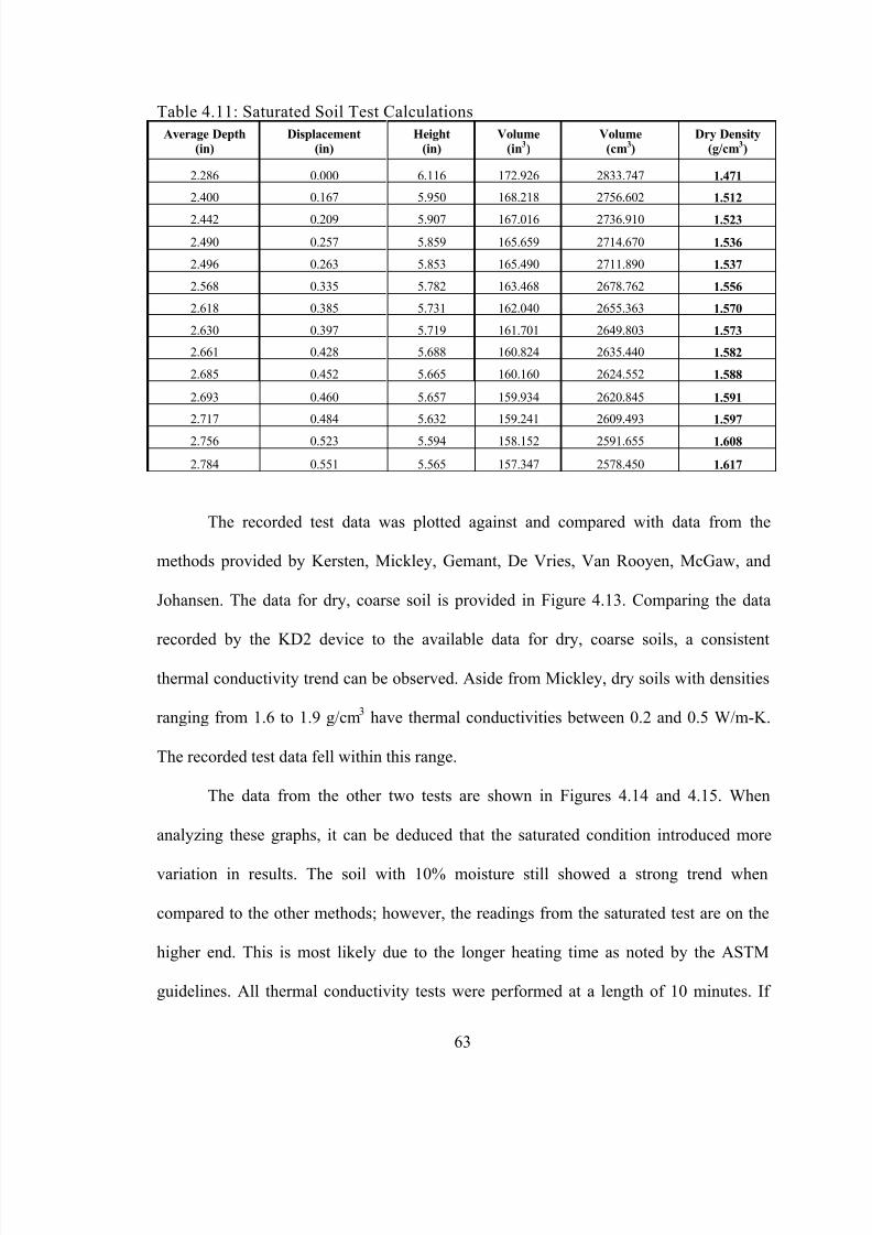
8/16/2019 Thermal Conductivity of Soils From the Analysis of Boring Logs
http://slidepdf.com/reader/full/thermal-conductivity-of-soils-from-the-analysis-of-boring-logs 74/96
63
Table 4.11: Saturated Soil Test CalculationsAverage Depth
(in)Displacement
(in)Height
(in)Volume
(in 3)Volume
(cm 3)Dry Density
(g/cm 3)
2.286 0.000 6.116 172.926 2833.747 1.471
2.400 0.167 5.950 168.218 2756.602 1.512
2.442 0.209 5.907 167.016 2736.910 1.523
2.490 0.257 5.859 165.659 2714.670 1.536
2.496 0.263 5.853 165.490 2711.890 1.537
2.568 0.335 5.782 163.468 2678.762 1.556
2.618 0.385 5.731 162.040 2655.363 1.570
2.630 0.397 5.719 161.701 2649.803 1.573
2.661 0.428 5.688 160.824 2635.440 1.582
2.685 0.452 5.665 160.160 2624.552 1.588
2.693 0.460 5.657 159.934 2620.845 1.591
2.717 0.484 5.632 159.241 2609.493 1.597
2.756 0.523 5.594 158.152 2591.655 1.608
2.784 0.551 5.565 157.347 2578.450 1.617
The recorded test data was plotted against and compared with data from the
methods provided by Kersten, Mickley, Gemant, De Vries, Van Rooyen, McGaw, and
Johansen. The data for dry, coarse soil is provided in Figure 4.13. Comparing the data
recorded by the KD2 device to the available data for dry, coarse soils, a consistent
thermal conductivity trend can be observed. Aside from Mickley, dry soils with densities
ranging from 1.6 to 1.9 g/cm 3 have thermal conductivities between 0.2 and 0.5 W/m-K.
The recorded test data fell within this range.
The data from the other two tests are shown in Figures 4.14 and 4.15. When
analyzing these graphs, it can be deduced that the saturated condition introduced more
variation in results. The soil with 10% moisture still showed a strong trend when
compared to the other methods; however, the readings from the saturated test are on the
higher end. This is most likely due to the longer heating time as noted by the ASTM
guidelines. All thermal conductivity tests were performed at a length of 10 minutes. If
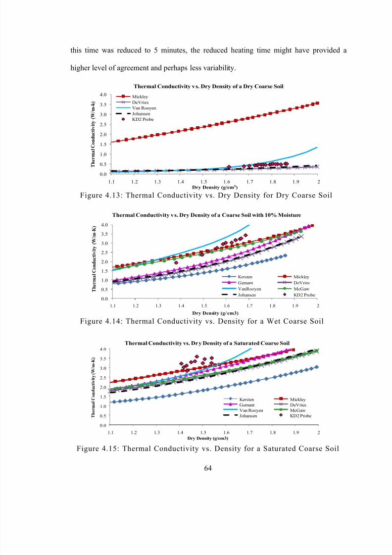
8/16/2019 Thermal Conductivity of Soils From the Analysis of Boring Logs
http://slidepdf.com/reader/full/thermal-conductivity-of-soils-from-the-analysis-of-boring-logs 75/96
64
this time was reduced to 5 minutes, the reduced heating time might have provided a
higher level of agreement and perhaps less variability.
Figure 4.13: Thermal Conductivity vs. Dry Density for Dry Coarse Soil
Figure 4.14: Thermal Conductivity vs. Density for a Wet Coarse Soil
Figure 4.15: Thermal Conductivity vs. Density for a Saturated Coarse Soil
0.0
0.5
1.0
1.5
2.0
2.5
3.0
3.54.0
1.1 1.2 1.3 1.4 1.5 1.6 1.7 1.8 1.9 2
T h e r m a l C o n d u c t i v i t y
( W / m - k )
Dry Density (g/cm 3 )
Thermal Conductivity v s. Dry Density of a Dry Coarse Soil
MickleyDeVriesVan RooyenJohansenKD2 Probe
0.00.5
1.0
1.5
2.0
2.5
3.0
3.5
4.0
1.1 1.2 1.3 1.4 1.5 1.6 1.7 1.8 1.9 2
T
h e r m a l C o n d u c t i v i t y
( W / m - K
)
Dry Density (g/ cm3)
Thermal Conductivity v s. Dry Density of a Coarse Soil with 10% Moisture
Kersten MickleyGemant DeVriesVanRooyen McGawJohansen KD2 Probe
0.0
0.5
1.0
1.52.0
2.5
3.0
3.5
4.0
1.1 1.2 1.3 1.4 1.5 1.6 1.7 1.8 1.9 2
T h e r m a l C o n d u c t i v i t y
( W / m - K
)
Dry Density (g/cm3)
Thermal Conductivity vs. Dry Density of a Saturated Coarse Soil
Kersten MickleyGemant DeVriesVan Rooyen McGawJohansen KD2 Probe
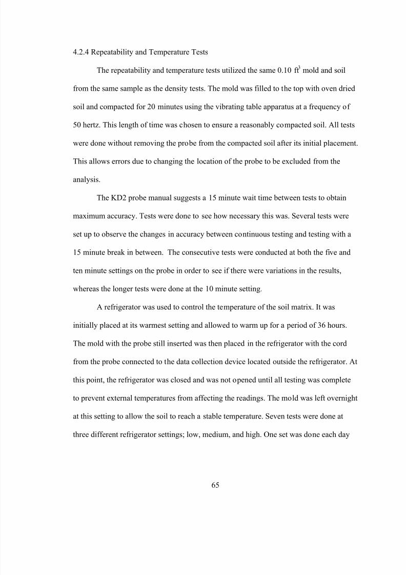
8/16/2019 Thermal Conductivity of Soils From the Analysis of Boring Logs
http://slidepdf.com/reader/full/thermal-conductivity-of-soils-from-the-analysis-of-boring-logs 76/96
65
4.2.4 Repeatability and Temperature Tests
The repeatability and temperature tests utilized the same 0.10 ft 3 mold and soil
from the same sample as the density tests. The mold was filled to the top with oven dried
soil and compacted for 20 minutes using the vibrating table apparatus at a frequency of
50 hertz. This length of time was chosen to ensure a reasonably compacted soil. All tests
were done without removing the probe from the compacted soil after its initial placement.
This allows errors due to changing the location of the probe to be excluded from the
analysis.
The KD2 probe manual suggests a 15 minute wait time between tests to obtainmaximum accuracy. Tests were done to see how necessary this was. Several tests were
set up to observe the changes in accuracy between continuous testing and testing with a
15 minute break in between. The consecutive tests were conducted at both the five and
ten minute settings on the probe in order to see if there were variations in the results,
whereas the longer tests were done at the 10 minute setting.
A refrigerator was used to control the temperature of the soil matrix. It was
initially placed at its warmest setting and allowed to warm up for a period of 36 hours.
The mold with the probe still inserted was then placed in the refrigerator with the cord
from the probe connected to the data collection device located outside the refrigerator. At
this point, the refrigerator was closed and was not opened until all testing was complete
to prevent external temperatures from affecting the readings. The mold was left overnight
at this setting to allow the soil to reach a stable temperature. Seven tests were done at
three different refrigerator settings; low, medium, and high. One set was done each day
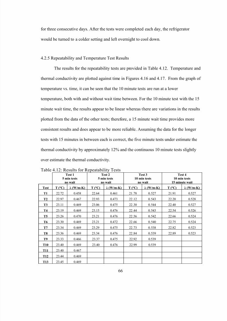
8/16/2019 Thermal Conductivity of Soils From the Analysis of Boring Logs
http://slidepdf.com/reader/full/thermal-conductivity-of-soils-from-the-analysis-of-boring-logs 77/96
66
for three consecutive days. After the tests were completed each day, the refrigerator
would be turned to a colder setting and left overnight to cool down.
4.2.5 Repeatability and Temperature Test Results
The results for the repeatability tests are provided in Table 4.12. Temperature and
thermal conductivity are plotted against time in Figures 4.16 and 4.17. From the graph of
temperature vs. time, it can be seen that the 10 minute tests are run at a lower
temperature, both with and without wait time between. For the 10 minute test with the 15
minute wait time, the results appear to be linear whereas there are variations in the results
plotted from the data of the other tests; therefore, a 15 minute wait time provides more
consistent results and does appear to be more reliable. Assuming the data for the longer
tests with 15 minutes in between each is correct, the five minute tests under estimate the
thermal conductivity by approximately 12% and the continuous 10 minute tests slightly
over estimate the thermal conductivity.
Table 4.12: Results for Repeatability TestsTest 1
5 min testsno wait
Test 25 min tests
no wait
Test 310 min tests
no wait
Test 410 min tests
15 minute wait
Test T (°C) λ (W/m -K) T (°C) λ (W/m -K) T (°C) λ (W/m -K) T (°C) λ (W/m -K)
T1 22.72 0.458 22.64 0.461 21.78 0.527 21.91 0.527
T2 22.97 0.467 22.93 0.473 22.12 0.543 22.20 0.528
T3 23.11 0.469 23.06 0.475 22.30 0.544 22.40 0.527
T4 23.19 0.469 23.15 0.476 22.44 0.543 22.54 0.526
T5 23.26 0.470 23.21 0.476 22.56 0.542 22.66 0.524
T6 23.30 0.469 23.21 0.472 22.66 0.540 22.75 0.524
T7 23.34 0.469 23.29 0.475 22.73 0.538 22.82 0.523
T8 23.36 0.469 23.34 0.476 22.84 0.539 22.89 0.523
T9 23.33 0.466 23.37 0.475 22.92 0.539
T10 23.40 0.469 23.40 0.476 22.99 0.539
T11 23.40 0.467
T12 23.44 0.469
T13 23.45 0.469
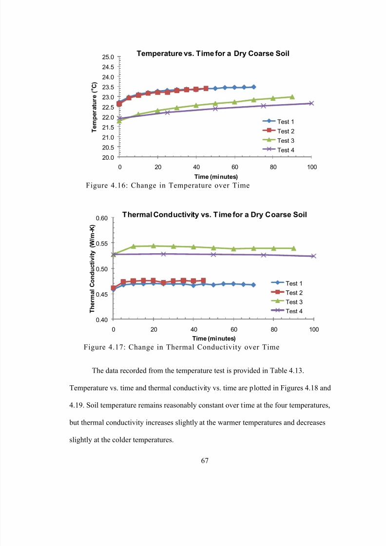
8/16/2019 Thermal Conductivity of Soils From the Analysis of Boring Logs
http://slidepdf.com/reader/full/thermal-conductivity-of-soils-from-the-analysis-of-boring-logs 78/96
67
Figure 4.16: Change in Temperature over Time
Figure 4.17: Change in Thermal Conductivity over Time
The data recorded from the temperature test is provided in Table 4.13.
Temperature vs. time and thermal conductivity vs. time are plotted in Figures 4.18 and
4.19. Soil temperature remains reasonably constant over time at the four temperatures,
but thermal conductivity increases slightly at the warmer temperatures and decreases
slightly at the colder temperatures.
20.0
20.5
21.0
21.5
22.0
22.5
23.0
23.5
24.0
24.5
25.0
0 20 40 60 80 100
T e m p e r a t u r e
( C )
Time (minutes)
Temperature vs. Time for a Dry Coarse Soil
Test 1
Test 2
Test 3
Test 4
0.40
0.45
0.50
0.55
0.60
0 20 40 60 80 100
T h e r m a l C
o n
d u c t i v i t y
( W / m - K
)
Time (minutes)
Thermal Conductivity vs. T ime for a Dry Coarse Soil
Test 1Test 2Test 3Test 4
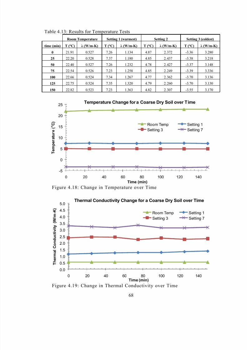
8/16/2019 Thermal Conductivity of Soils From the Analysis of Boring Logs
http://slidepdf.com/reader/full/thermal-conductivity-of-soils-from-the-analysis-of-boring-logs 79/96
68
Table 4.13: Results for Temperature Tests
Room Temperature Setting 1 (warmest) Setting 2 Setting 3 (coldest)
time (min) T (°C) λ (W/m -K) T (°C) λ (W/m -K) T (°C) λ (W/m -K) T (°C) λ (W/m -K)
0 21.91 0.527 7.26 1.134 4.87 2.372 -3.36 3.280
25 22.20 0.528 7.37 1.180 4.85 2.437 -3.38 3.218
50 22.40 0.527 7.26 1.232 4.78 2.427 -3.37 3.148
75 22.54 0.526 7.23 1.258 4.85 2.249 -3.39 3.336
100 22.66 0.524 7.34 1.267 4.77 2.362 -3.70 3.136
125 22.75 0.524 7.35 1.320 4.79 2.260 -3.70 3.130
150 22.82 0.523 7.23 1.363 4.82 2.307 -3.55 3.170
Figure 4.18: Change in Temperature over Time
Figure 4.19: Change in Thermal Conductivity over Time
-5
0
5
10
15
20
25
0 20 40 60 80 100 120 140
T e m p e r a t u r e
( C )
Time (min)
Temperature Change for a Coarse Dry Soil over Time
Room Temp Setting 1Setting 3 Setting 7
0.0
0.5
1.0
1.52.0
2.5
3.0
3.5
4.0
4.5
5.0
0 20 40 60 80 100 120 140
T h e r m a l C o n
d u c t i v i t y
( W / m - K
)
Time (min)
Thermal Conductivity Change for a Coarse Dry Soil over Time
Room Temp Setting 1Setting 3 Setting 7

8/16/2019 Thermal Conductivity of Soils From the Analysis of Boring Logs
http://slidepdf.com/reader/full/thermal-conductivity-of-soils-from-the-analysis-of-boring-logs 80/96
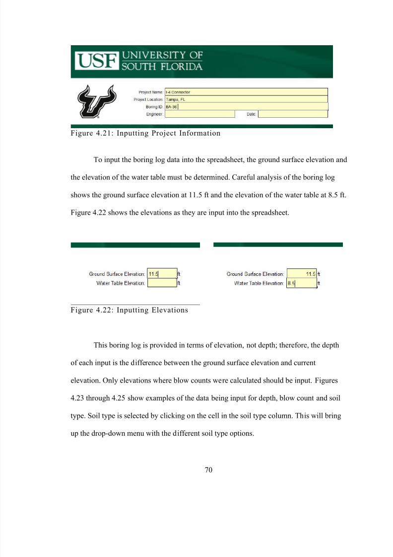
8/16/2019 Thermal Conductivity of Soils From the Analysis of Boring Logs
http://slidepdf.com/reader/full/thermal-conductivity-of-soils-from-the-analysis-of-boring-logs 81/96
70
Figure 4.21: Inputting Project Information
To input the boring log data into the spreadsheet, the ground surface elevation and
the elevation of the water table must be determined. Careful analysis of the boring log
shows the ground surface elevation at 11.5 ft and the elevation of the water table at 8.5 ft.
Figure 4.22 shows the elevations as they are input into the spreadsheet.
Figure 4.22: Inputting Elevations
This boring log is provided in terms of elevation, not depth; therefore, the depth
of each input is the difference between the ground surface elevation and current
elevation. Only elevations where blow counts were calculated should be input. Figures
4.23 through 4.25 show examples of the data being input for depth, blow count and soil
type. Soil type is selected by clicking on the cell in the soil type column. This will bring
up the drop-down menu with the different soil type options.
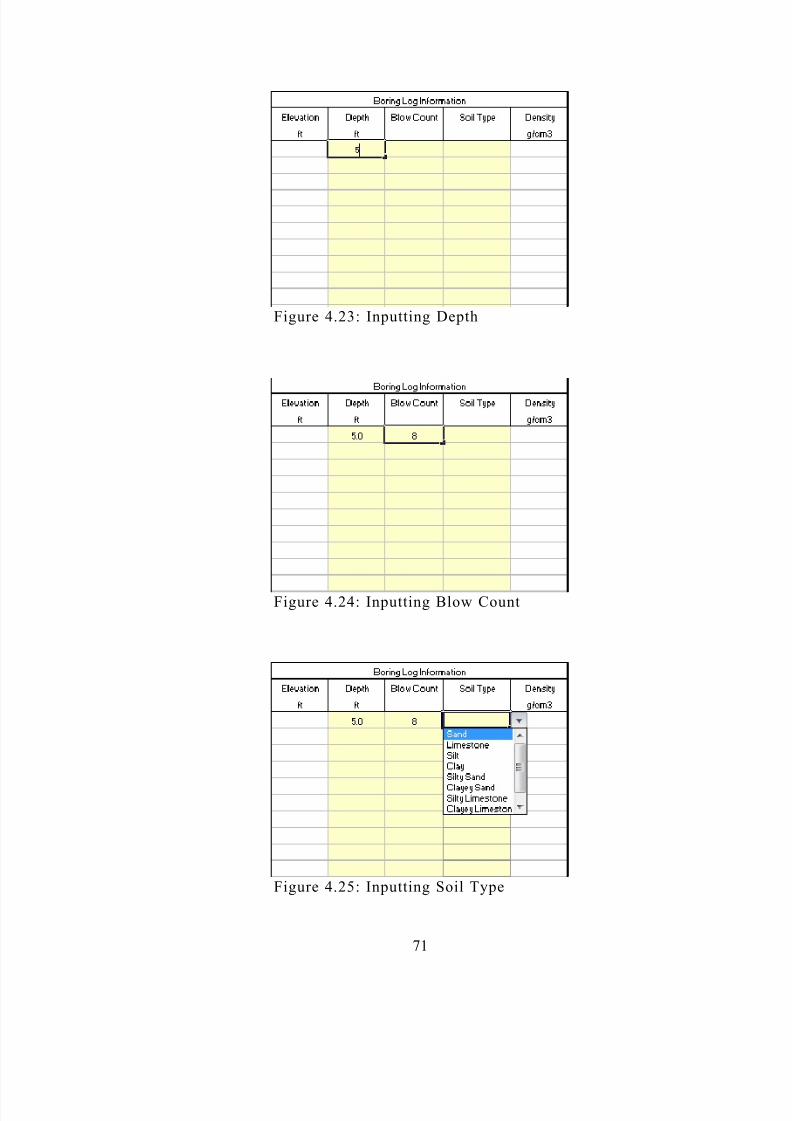
8/16/2019 Thermal Conductivity of Soils From the Analysis of Boring Logs
http://slidepdf.com/reader/full/thermal-conductivity-of-soils-from-the-analysis-of-boring-logs 82/96
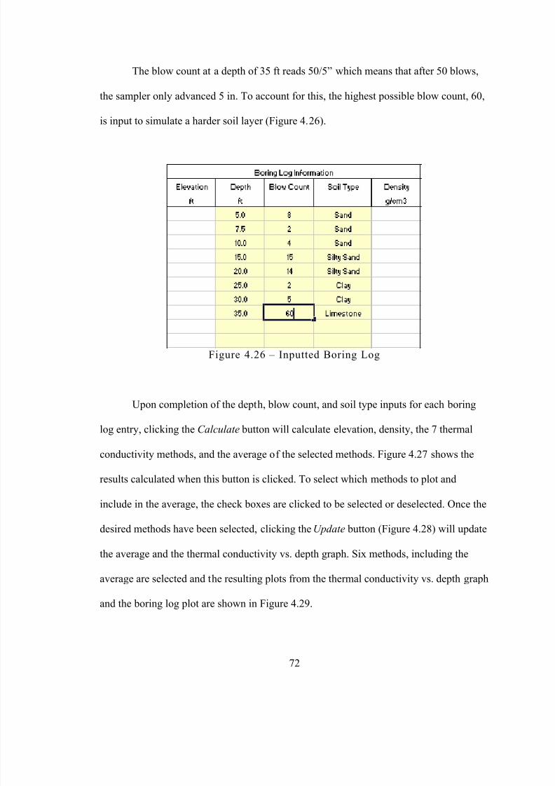
8/16/2019 Thermal Conductivity of Soils From the Analysis of Boring Logs
http://slidepdf.com/reader/full/thermal-conductivity-of-soils-from-the-analysis-of-boring-logs 83/96
72
The blow count at a depth of 35 ft reads 50/5” which means that after 50 blows,
the sampler only advanced 5 in. To account for this, the highest possible blow count, 60,
is input to simulate a harder soil layer (Figure 4.26).
Figure 4.26 – Inputted Boring Log
Upon completion of the depth, blow count, and soil type inputs for each boring
log entry, clicking the Calculate button will calculate elevation, density, the 7 thermal
conductivity methods, and the average of the selected methods. Figure 4.27 shows the
results calculated when this button is clicked. To select which methods to plot and
include in the average, the check boxes are clicked to be selected or deselected. Once the
desired methods have been selected, clicking the Update button (Figure 4.28) will update
the average and the thermal conductivity vs. depth graph. Six methods, including the
average are selected and the resulting plots from the thermal conductivity vs. depth graph
and the boring log plot are shown in Figure 4.29.
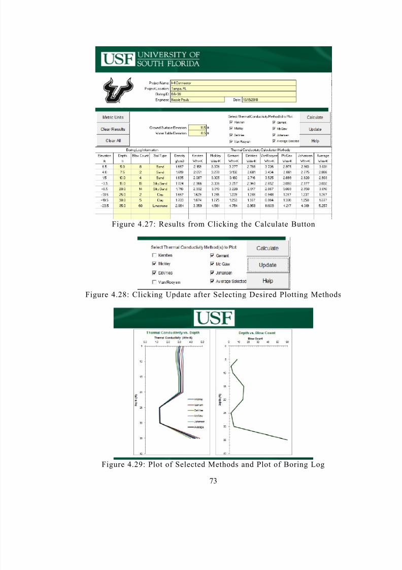
8/16/2019 Thermal Conductivity of Soils From the Analysis of Boring Logs
http://slidepdf.com/reader/full/thermal-conductivity-of-soils-from-the-analysis-of-boring-logs 84/96
73
Figure 4.27: Results from Clicking the Calculate Button
Figure 4.28: Clicking Update after Selecting Desired Plotting Methods
Figure 4.29: Plot of Selected Methods and Plot of Boring Log

8/16/2019 Thermal Conductivity of Soils From the Analysis of Boring Logs
http://slidepdf.com/reader/full/thermal-conductivity-of-soils-from-the-analysis-of-boring-logs 85/96
74
4.3.1 Heat Capacity
As the ultimate thermal property controlling diffusion is diffusivity, an additional
module was created to compute the heat capacity from which the diffusivity can be
calculated for each boring log entry using the following equation from chapter 2.
Heat capacity, C, is a far less intense computation requiring only the fraction of
air, water, and soil as well as the mineralogy. This is calculated using the equation for
specific heat,
where C S, C w, and C a are the heat capacities of soil, water, and air, and X S, X W, and X a
are the volumetric fractions of soil, water, and air (Duarte 2006).
8/16/2019 Thermal Conductivity of Soils From the Analysis of Boring Logs
http://slidepdf.com/reader/full/thermal-conductivity-of-soils-from-the-analysis-of-boring-logs 86/96
75
Chapter 5 - Conclusion
Thermal properties of soils vary drastically depending on the mineralogy, density,
saturation state, and structure. Despite several decades of research on the topic, no
rational correlations exist that predict thermal properties using common soil exploration
methods. This thesis focused on assembling correlations from existing literature to close
the gap between SPT sampling and thermal properties. The direct applications of defining
the thermal properties of soils include both geothermal heating/cooling systems and thosemethods of foundation quality assurance involving thermal integrity profiling. The latter
of which is discussed below.
5.1 Thermal In tegrity Profil in g
Thermal integrity profiling is a test method that assesses the intactness of cast-in-
place concrete with emphasis on an underground structural element (e.g. drilled shaft or
ACIP). The hydration energy of curing concrete is sufficient in magnitude to develop a
temperature signature relative to the volume of concrete placed. In cases where the soil is
uniform, the developed temperature is also uniform for a perfectly shaped cylinder.
Variations in cross section can cause increases or decreases in the measured temperature
proportional to bulges or necks, respectively.
Figures 5.1 through 5.3 show the temperature variation from TIP testing of shafts
constructed with permanent casing in the upper portion along with the SPT blow counts.
These three shafts provide an interesting case study for this thesis as the cross section is
known not to have varied. As a result, the temperature variations recorded are largely the
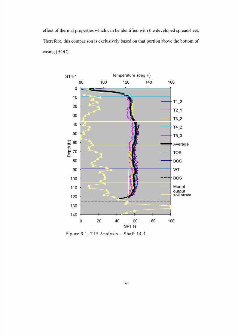
8/16/2019 Thermal Conductivity of Soils From the Analysis of Boring Logs
http://slidepdf.com/reader/full/thermal-conductivity-of-soils-from-the-analysis-of-boring-logs 87/96
76
effect of thermal properties which can be identified with the developed spreadsheet.
Therefore, this comparison is exclusively based on that portion above the bottom of
casing (BOC).
Figure 5.1: TIP Analysis – Shaft 14-1
0 20 40 60 80 100
0
10
20
30
40
50
60
70
80
90
100
110
120
130
140
80 100 120 140 160
SPT N
D e p
t h ( f t )
Temperature (deg F)
T1_2
T2_1
T3_2
T4_2
T5_3
Average
TOS
BOC
WT
BOS
Modeloutputsoil strata
S14-1
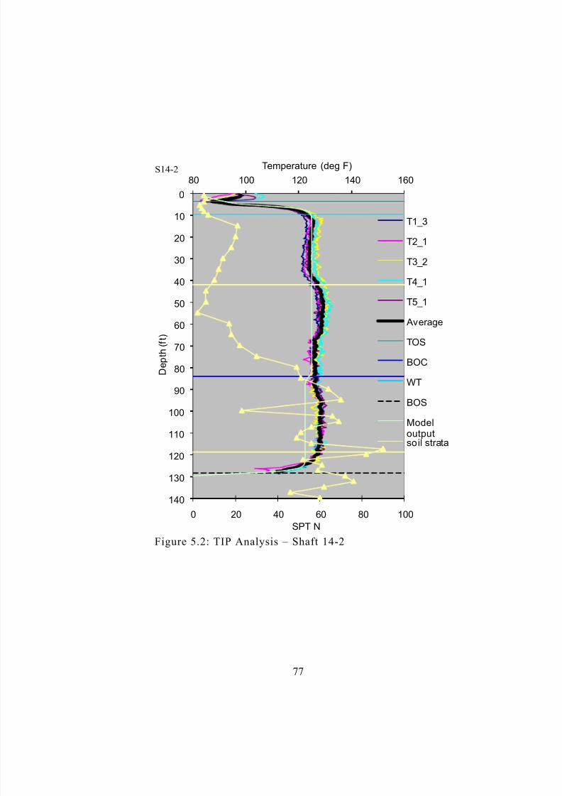
8/16/2019 Thermal Conductivity of Soils From the Analysis of Boring Logs
http://slidepdf.com/reader/full/thermal-conductivity-of-soils-from-the-analysis-of-boring-logs 88/96
77
Figure 5.2: TIP Analysis – Shaft 14-2
0 20 40 60 80 100
0
10
20
30
40
50
60
70
80
90
100
110
120
130
140
80 100 120 140 160
SPT N
D e p
t h ( f t )
Temperature (deg F)
T1_3
T2_1
T3_2
T4_1
T5_1
Average
TOS
BOC
WT
BOS
Modeloutputsoil strata
S14-2

8/16/2019 Thermal Conductivity of Soils From the Analysis of Boring Logs
http://slidepdf.com/reader/full/thermal-conductivity-of-soils-from-the-analysis-of-boring-logs 89/96
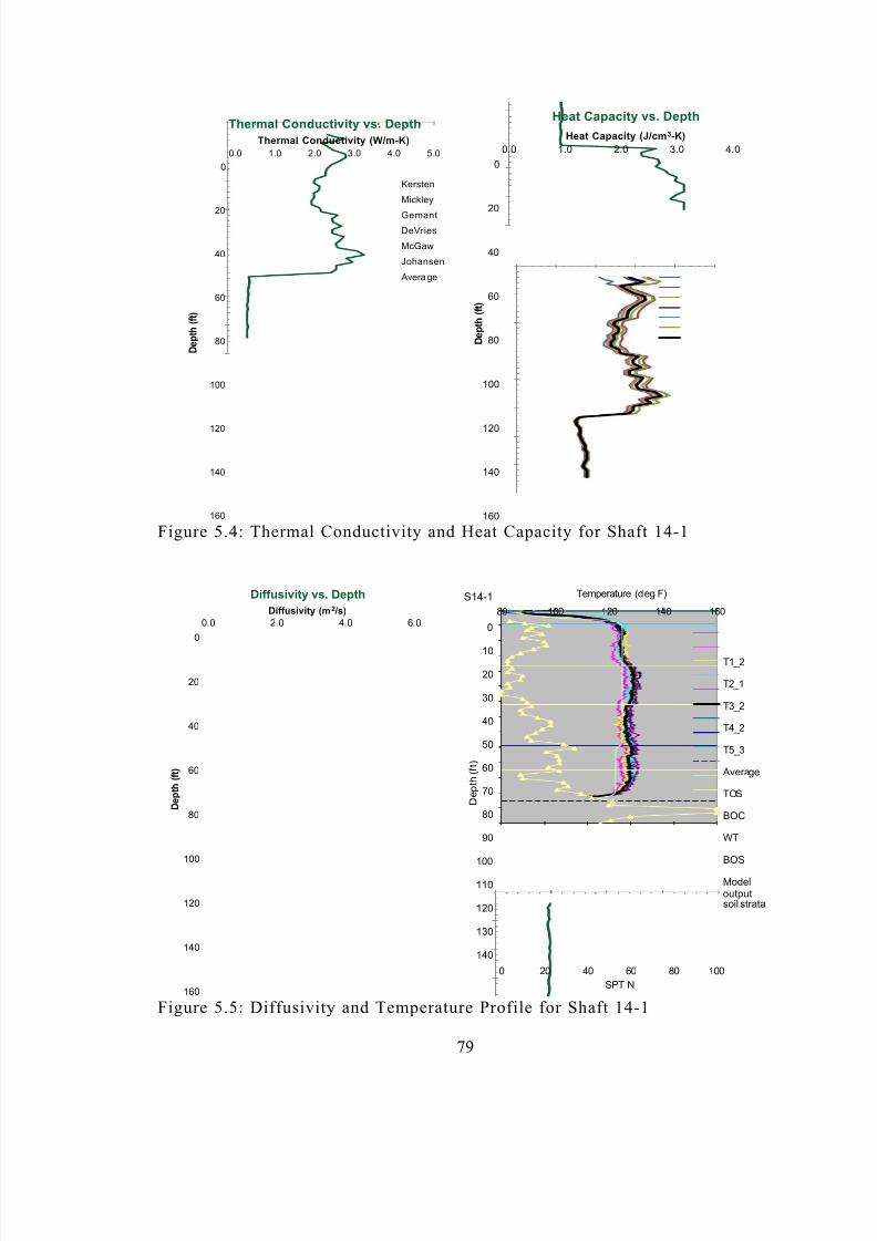
8/16/2019 Thermal Conductivity of Soils From the Analysis of Boring Logs
http://slidepdf.com/reader/full/thermal-conductivity-of-soils-from-the-analysis-of-boring-logs 90/96
79
Figure 5.4: Thermal Conductivity and Heat Capacity for Shaft 14-1
Figure 5.5: Diffusivity and Temperature Profile for Shaft 14-1
0
20
40
60
80
100
120
140
160
0.0 1.0 2.0 3.0 4.0 5.0
D e p t h ( f t )
Thermal Conductivity (W/m-K)
Thermal Conductivity vs. Depth
Kersten
Mickley
GemantDeVries
McGaw
Johansen
Avera ge
0
20
40
60
80
100
120
140
160
0.0 1.0 2.0 3.0 4.0
D e p t h
( f t )
Heat Capacity (J/cm 3-K)
Heat Capacity vs. Depth
0
20
40
60
80
100
120
140
160
0.0 2.0 4.0 6.0
D e p
t h ( f t )
Diffusivity (m 2 /s)
Diffusivity vs. Depth
0 20 40 60 80 100
0
10
20
30
40
50
60
70
80
90
100
110
120
130
140
80 100 120 140 160
SPT N
D e p
t h ( f t )
Temperature (deg F)
T1_2
T2_1
T3_2
T4_2
T5_3
Average
TOS
BOC
WT
BOS
Modeloutputsoil strata
S14-1
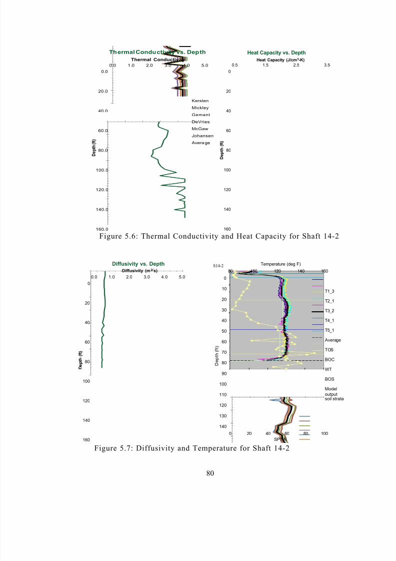
8/16/2019 Thermal Conductivity of Soils From the Analysis of Boring Logs
http://slidepdf.com/reader/full/thermal-conductivity-of-soils-from-the-analysis-of-boring-logs 91/96
80
Figure 5.6: Thermal Conductivity and Heat Capacity for Shaft 14-2
Figure 5.7: Diffusivity and Temperature for Shaft 14-2
0.0
20.0
40.0
60.0
80.0
100.0
120.0
140.0
160.0
0.0 1.0 2.0 3.0 4.0 5.0
D e p t h ( f t )
Thermal Conductivity
Th ermal Condu ctivity vs. Dep th
Kersten
Mickley
Gemant
DeVries
McGaw
Johansen
Avera ge
0
20
40
60
80
100
120
140
160
0.5 1.5 2.5 3.5
D e p t h
( f t )
Heat Capacity (J/cm 3-K)
Heat Capacity vs. Depth
0
20
40
60
80
100
120
140
160
0.0 1.0 2.0 3.0 4.0 5.0
D e p t h
( f t )
Diffusivity (m 2/ s)Diffusivity vs. Depth
0 20 40 60 80 100
0
10
20
30
40
50
60
70
80
90
100
110
120
130
140
80 100 120 140 160
SPT N
D e p
t h ( f t )
Temperature (deg F)
T1_3
T2_1
T3_2
T4_1
T5_1
Average
TOS
BOC
WT
BOS
Modeloutputsoil strata
S14-2
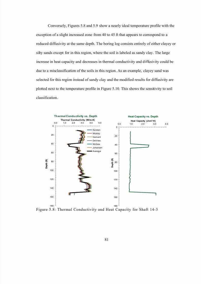
8/16/2019 Thermal Conductivity of Soils From the Analysis of Boring Logs
http://slidepdf.com/reader/full/thermal-conductivity-of-soils-from-the-analysis-of-boring-logs 92/96
81
Conversely, Figures 5.8 and 5.9 show a nearly ideal temperature profile with the
exception of a slight increased zone from 40 to 45 ft that appears to correspond to a
reduced diffusivity at the same depth. The boring log consists entirely of either clayey or
silty sands except for in this region, where the soil is labeled as sandy clay. The large
increase in heat capacity and decreases in thermal conductivity and diffusivity could be
due to a misclassification of the soils in this region. As an example, clayey sand was
selected for this region instead of sandy clay and the modified results for diffusivity are
plotted next to the temperature profile in Figure 5.10. This shows the sensitivity to soil
classification.
Figure 5.8: Thermal Conductivity and Heat Capacity for Shaft 14-3
0
20
40
60
80
100
120
140
160
180
0.0 1.0 2.0 3.0 4.0 5.0
D e p t h
( f t )
Thermal Conductivity (W/m-K)
Th ermal Condu ctivity vs. Depth
Kersten
Mickley
Gemant
DeVries
McGaw
Johansen
Averag e
0
20
40
60
80
100
120
140
160
180
0.0 1.0 2.0 3.0 4.0
D e p t h
( f t )
Heat Capacity (J/cm 3-K)
Heat Capacity vs. Depth
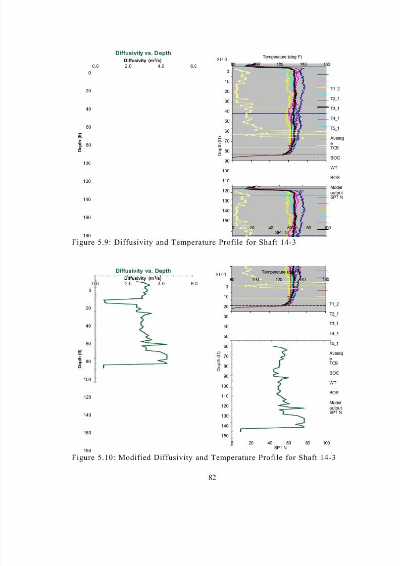
8/16/2019 Thermal Conductivity of Soils From the Analysis of Boring Logs
http://slidepdf.com/reader/full/thermal-conductivity-of-soils-from-the-analysis-of-boring-logs 93/96
82
Figure 5.9: Diffusivity and Temperature Profile for Shaft 14-3
Figure 5.10: Modified Diffusivity and Temperature Profile for Shaft 14-3
0
20
40
60
80
100
120
140
160
180
0.0 2.0 4.0 6.0
D e p t h
( f t )
Diffusivity (m 2 /s)
Diffusivity vs. Depth
0 20 40 60 80 100
0
10
20
30
40
50
60
70
80
90
100
110
120
130
140
150
80 100 120 140 160
SPT N
D e p
t h ( f t )
Temperature (deg F)
T1_2
T2_1
T3_1
T4_1
T5_1
AverageTOS
BOC
WT
BOS
Modeloutput
SPT N
S14-3
0
20
40
60
80
100
120
140
160
180
0.0 2.0 4.0 6.0
D e p t h
( f t )
Diffusivity (m 2 /s)
Diffusivity vs. Depth
0 20 40 60 80 100
0
10
20
30
40
50
60
70
80
90
100
110
120
130
140
150
80 100 120 140 160
SPT N
D e p
t h ( f t )
Temperature (deg F)
T1_2
T2_1
T3_1
T4_1
T5_1
AverageTOS
BOC
WT
BOS
ModeloutputSPT N
S14-3
8/16/2019 Thermal Conductivity of Soils From the Analysis of Boring Logs
http://slidepdf.com/reader/full/thermal-conductivity-of-soils-from-the-analysis-of-boring-logs 94/96
83
Obviously, limitations exist in such an approach in that often times the nearest
boring log may not reflect the actual conditions. In those cases, construction logs can be
used to explain subtle variations in soil mineralogy, but can only qualitatively assess the
effect.
5.2 Futu re Studies
At present, efforts are underway to develop a CPT-based thermal conductivity
probe. This has the potential to more readily quantify both the soil characteristics (i.e.
strength, structure, and mineralogy) and the thermal conductivity with vertical depth
resolution for more precise measurements (1 data point/cm) than the SPT wherein 1 data
point per 1.5 ft is the absolute finest resolution attainable.
5.3 Summar y
This thesis presents a new analysis tool for the purpose of quantifying the thermal
properties of soil from commonly used SPT boring log data. It is thought to be the only
such attempt to do so and as such will likely incur numerous changes and refinements in
ensuing years. The applicability of the thesis findings are at present somewhat limited but
predictive methods in these areas are receiving much needed attention and will benefit
from the inroads developed herein.
8/16/2019 Thermal Conductivity of Soils From the Analysis of Boring Logs
http://slidepdf.com/reader/full/thermal-conductivity-of-soils-from-the-analysis-of-boring-logs 95/96
84
List of References
ASTM (1996) , “Annual Book of ASTM Standards”, Vol. 4.08, D1586, D4253, D4318
ASTM (2008 ), “Annual Book of ASTM Standards”, Vol. 4.08, D5334
Duarte, A., Campos, T., Araruna, J., and Filho, P., (2006). “Thermal Properties of Unsaturated Soils,” Unsaturated Soils , GSP, ASCE, pp. 1707-1718.
Earth Temperature and Site Geology. Virginia Tech, Department of Mines Minerals andEnergy. Web.http://www.geo4va.vt.edu/A1/A1.htm
Farouki, O. ( 1982). “Evaluation of Methods for Calculating Soil Thermal Conductivity,”Report 82-8, US Army Corps of Engineers Cold Regions Research and EngineeringLaboratory, pp. 14-23
Farouki, O. ( 1966). “Physical Properties of Granular Materials with Reference to Thermal Resistivi ty,” Highway Research Record 128, National Research Council, Washington, DC, pp. 25-44
Johansen, O. (1977). “Thermal Conductivity of Soils,” U.S. Army Corps of EngineersCold Regions Research and Engineering Laboratory. Hanover, NH, pp. 1-46
Johansen, O. (1975). “Thermal Conductivity of Soils and Rocks,” Proceedings of the Sixth International Congress of the Foundation Francaise d’Etudes Nordigues, Vol. 2,
pp.407-420
Kersten, M.S. (1949 ). “Thermal Properties of Soils,” University of Minnesota Institut e ofTechnology, Engineering Experiment Station, Vol. LII, No. 21.
Kranc, S.C. and Mullins, G. (2007). “Inverse Method for the Detection of Voids inDrilled Shaft Concrete Piles from Longitudinal Temperature Scans,” Inverse ProblemsDesign and Optimization Symposium, Miami, FL, April 16-18, 2007.
8/16/2019 Thermal Conductivity of Soils From the Analysis of Boring Logs
http://slidepdf.com/reader/full/thermal-conductivity-of-soils-from-the-analysis-of-boring-logs 96/96
Kulhawy, F. H. and Mayne, P. W. (1990), “Manual on Estimating Soil Properties forFoundation Design,” Technical Report EPRI -EL-6800, Electric Power Research Institute,Palo Alto, CA.
Limestone Properties. University of Florida. Bridge Software Institute. Web.http://bsi-web.ce.ufl.edu/downloads/files/MultiPier_Soil_Table.pdf
Maynard, Whitney (2010). “Monitoring and Evaluation of Geothermal Systems,”Master’s Thesis, University of South Florida, December.
Mullins, G., Winters, D., and Johnson, K., (2009), "Attenuating Mass Concrete Effects in
Drilled Shafts," Final Report, FDOT Project BD544-39, September.Mullins, G. and Kranc, S., (2007), "Thermal Integrity Testing of Drilled Shafts," FinalReport, FDOT Project BD544-20, May.
Mullins, G. and Ashmawy, A., (2005), "Factors Affecting Anomaly Formation in DrilledShafts," Final Report, FDOT Project BC353-19, March.
Mullins, A. G. and Kranc, S. C., (2004), “Method for Testing the Integrity of ConcreteShafts,” US Patent 6,783,273.
Mullins, G. and Winters, D. (2004). "Post Grouting Drilled Shaft Tips - Phase II FinalReport." Final Report submitted Florida Department of Transportation, June.
Trout, K. (2010). “ Integrated North Tampa Bay Model Application of the IntegratedHydrologic Model,” INTB Model Calibration Report, Tampa Bay Water. In press.