PROGRESS TOWARDS THE INTELLIGENT CONTROL OF A

POWERED TRANSFEMORAL PROSTHESIS

By

Huseyin Atakan Varol

Thesis

Submitted to the Faculty of the

Graduate School of Vanderbilt University in

partial fulfillment of the requirements

for the degree of

MASTER OF SCIENCE

in

Electrical Engineering

August, 2007

Nashville, Tennessee

Approved:

Professor Michael Goldfarb

Professor D. Mitch Wilkes

Professor George E. Cook

ii

To my family

iii

ACKNOWLEDGMENTS

First and foremost, I would like to thank my advisor Professor Michael Goldfarb for his inspiration,

guidance, patience and encouragement throughout the duration of my thesis. He will be always a role

model for my academic career. I would also like to express my appreciation and gratitude to Professor

Mitch Wilkes and Professor George E. Cook for letting me to have them as members of my thesis

committee.

This work would not have been possible without the grants of the National Science Foundation and

the National Institutes of Health . Hereby, I greatly acknowledge both organisations for their support.

Thanks also go to all my colleagues at the Center for Intelligent Mechatronics. Post doctoral research

associates Dr. Kevin Fite and Dr. Tom Withrow have been invaluable for their advice and assistance

throughout my masters work. In particular, I would like to acknowledge Frank C. Sup for his contributions

to my work and his outstanding advice and critique. I would also like to acknowledge David Slifer for his

help during his summer internship. Moreover, I would like to thank David Braun for our informative and

challenging technical discussions during the breaks.

I also wanted to thank those who shared joys and sorrows throuhgout my stay at Vanderbilt University:

Barbaros Cetin, Duygun Erol, Erdem Erdemir, Jonathan E. Hunter, Mert Tugcu and Tamim I. Sookoor. I

would like to express my sincere thanks to Gulnara Namyssova for always being with me and supporting

me whenever I needed. Furthermore, I would like to thank my parents, Huseyin Selcuk Varol and Gungor

Varol, and my brother Erkan Varol, whose love and trust I never lacked in my whole life.

iv

TABLE OF CONTENTS

Page

ACKNOWLEDGMENTS...................................................................................................................iii LIST OF FIGURES.......................................................................................................................... vi LIST OF TABLES ......................................................................................................................viii Chapter I. INTRODUCTION ........................................................................................................................1

1. Introduction .........................................................................................................1 2. Literature Survey.................................................................................................3 3. Motivation and Contribution ................................................................................6 4. Organization of the Document ............................................................................7 5. References..........................................................................................................8

II. MANUSCRIPT I: REAL-TIME INTENT RECOGNITION FOR A POWERED KNEE AND ANKLE

TRANSFEMORAL PROSTHESIS ....................................................................10

1. Abstract .......................................................................................................... 11 2. Introduction ....................................................................................................... 11 3. Prior Work in Powered Transfemoral Prosthesis..............................................13 4. Interface Approaches........................................................................................13 5. K-Nearest Neighbor Classification....................................................................16

5.1 K-Nearest Neighbor Algorithm .................................................. 17 5.2 Application of k-NN to Gait Mode Recognition ......................... 18

6. Implementation and Experimental Validation....................................................20 6.1 Gait Experiments ...................................................................... 20 6.2 Class Database and Generation of Test Sequences................ 23

7. Results and Discussion.....................................................................................25 8. Conclusion ........................................................................................................28 9. References........................................................................................................28

v

III. MANUSCRIPT II: DECOMPOSITION-BASED CONTROL FOR A POWERED KNEE AND ANKLE TRANSFEMORAL PROSTHESIS ....................................................................31

1. Abstract ..........................................................................................................32 2. Introduction .......................................................................................................32 3. Prior Work in Powered Transfemoral Prostheses.............................................33 4. Interface Approaches........................................................................................34 5. Decomposition-Based Control ..........................................................................36 6. Active Passive Torque Decomposition..............................................................38 7. Joint Torque Reference Generation..................................................................42 8. Implementation and Experimental Validation....................................................44 9. Results and Discussion.....................................................................................46 10. Conclusion ........................................................................................................48 11. References ........................................................................................................48

IV. THREE AXIS SOCKET LOAD CELL CALIBRATION................................................................51 APPENDIX A. MATLAB CODES.......................................................................................................................55

1. K-Nearest Neighbor Algorithm Main Script.......................................................55 2. Active-Passive Decomposition Procedure Main Script.....................................60 3. Three Axis Socket Load Cell Calibration Script ................................................70

B. SIMULINK MODELS..................................................................................................................72

vi

LIST OF FIGURES

Page Figure 1-1. Standard lower limp prostheses including mechanical damping

knee with locking and solid ankle cushioned heel (SACH) foot. .....................................1 Figure 1-2. The Ossur Rheo knee (left) and the Otto Bock C-Leg (right) represent

the cutting edge of microprocesser controlled damping prosthetic knees. .....................2 Figure 1-3. The Otto Bock Trias Foot represents a typical spring-action ankle. ...........................................3 Figure 1-4. Flowers et al. (circa 1970’s) developed a hydraulically actuated

knee prosthesis that pioneered the use of active joints...................................................4 Figure 1-5. Electromagnetically actuated powered knee developed by Popovic with a battery pack. .........5 Figure 1-6. Ossur "Proprio" foot actively positions the foot for increased functionality.................................5 Figure 1-7. Ossur "Power Knee" uses electromagnetic actuation, which limits the battery life....................5 Figure 2-1. Power knee and ankle prosthesis prototype. ...........................................................................12 Figure 2-2. Structure of the transfemoral prosthesis control system.. ........................................................17 Figure 2-3. Illustration of the k-NN algorithm for the classification of an unknown

example, ux , with 5 nearest neighbors and 4 classes...............................................18 Figure 2-4. Pseudocode of the k-NN based intent recognition algorithm. ..................................................20 Figure 2-5. Data collection for the demonstration of the proposed approach.............................................22 Figure 2-6. The hip torque (a), the ground reaction force (b), the knee angle (c),

the ankle angle (d), and the different walking modes (e) for an example walking trial scenario. ...........................................................................24

Figure 2-7. Effect of biasing constant on chattering and delay. ..................................................................26

vii

Figure 2-8. Mode estimation for a 30.42 seconds trial walking scenario with the (a) plain k-NN algorithm, (b) k-NN with the biasing constant, (c) k-NN with both the biasing constant and the time based majority voting.................27

Figure 3-1. Power knee and ankle prosthesis prototype. ...........................................................................33 Figure 3-2. Structure of the transfemoral prosthesis control system. .........................................................37 Figure 3-3. Normal speed walking phase portrait of the knee joint and four stride segments....................39 Figure 3-4. Selection and indexing of data samples from Segment 1. .......................................................41 Figure 3-5. The output of the decomposition for Segment 1 showing the

spring and dashpot constants and the active and passive knee torques (Spring origin, α .is 23 degrees.). ..............................................43

Figure 3-6. Structure of the switched control system..................................................................................43 Figure 3-7. Data collection for the demonstration of the proposed approach.............................................45 Figure 3-8. The angular position, angular velocity and torque of the knee joint

for a walking experiment with normal speed. ................................................................46 Figure 3-9. Original knee torque and the reconstructed knee torque reference

versus time (a) and the angular position (b). .................................................................47 Figure 4-1. Three axis socket load cell calibration setup............................................................................53 Figure 4-2. Axial force versus Estimated Axial Force .................................................................................53 Figure 4-3. Frontal moment versus Estimate frontal moment.....................................................................54 Figure 4-4. Sagittal plane moment versus estimated sagital plane moment. .............................................54

viii

LIST OF TABLES

Page

Table 2-1 Walking Experiment Parameters (1) ...............................................................................23

Table 2-2 Mode Identification Error for Different Parameters .........................................................26

Table 3-1 Walking Experiment Parameters (2) ...............................................................................45

1

CHAPTER I

INTRODUCTION

1. Introduction

The evolution of the lower limb prosthesis over the recent decades has progressed from purely

mechanical systems to systems that include microprocessor control. When evaluating the basic function

of standard mechanical knee prostheses, Figure 1-1, their function is to provide mechanical damping in

order to extract energy from the system and limit the flexion of the knee joint in the back swing to prevent a

collision of the knee joint at full extension. These devices allow for restricted mobility of amputees and

provide an abnormal gait pattern.

Figure 1-1. Standard lower limb prostheses including mechanical damping knee with locking and solid ankle cushioned heel (SACH) foot.

The current generation of lower limb prostheses, Figure 1-2, incorporate microprocessors to control

either electromagnetic brakes or magnetic rheological fluid for the modulation of the damping in the knee

throughout the gait cycle. The incorporation of spring elements in the ankle, Figure 1-3, provides some

power return in the gait cycle, but is incapable of producing net power. The devices do provide users with

2

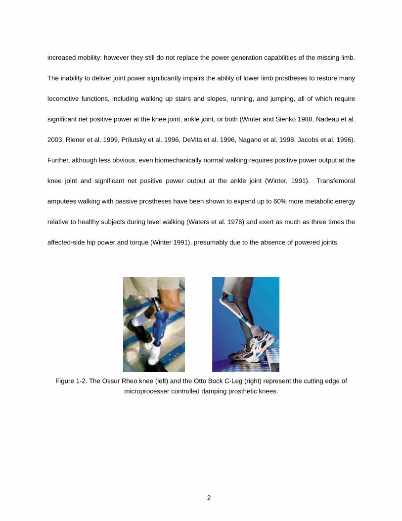
increased mobility; however they still do not replace the power generation capabilities of the missing limb.

The inability to deliver joint power significantly impairs the ability of lower limb prostheses to restore many

locomotive functions, including walking up stairs and slopes, running, and jumping, all of which require

significant net positive power at the knee joint, ankle joint, or both (Winter and Sienko 1988, Nadeau et al.

2003, Riener et al. 1999, Prilutsky et al. 1996, DeVita et al. 1996, Nagano et al. 1998, Jacobs et al. 1996).

Further, although less obvious, even biomechanically normal walking requires positive power output at the

knee joint and significant net positive power output at the ankle joint (Winter, 1991). Transfemoral

amputees walking with passive prostheses have been shown to expend up to 60% more metabolic energy

relative to healthy subjects during level walking (Waters et al. 1976) and exert as much as three times the

affected-side hip power and torque (Winter 1991), presumably due to the absence of powered joints.

Figure 1-2. The Ossur Rheo knee (left) and the Otto Bock C-Leg (right) represent the cutting edge of

microprocesser controlled damping prosthetic knees.

3

Figure 1-3. The Otto Bock Trias Foot represents a typical spring-action ankle.

A prosthesis with the capacity to deliver power at the knee and ankle joints would address these

deficiencies, and would additionally enable the restoration of biomechanically normal locomotion. Such a

prosthesis, however, would require 1) power generation capabilities comparable to an actual limb and 2) a

control framework for generating required joint torques for locomotion while ensuring stable and

coordinated interaction with the user and the environment.

2. Literature Survey

Prior work does exists on the development of powered knee transfemoral prostheses and powered

ankle transtibial prostheses. Flowers (1973), Donath (1974), Flowers and Mann (1977), Grimes et al.

(1977), Grimes (1979), Stein (1983), and Stein and Flowers (1988) developed a tethered electrohydraulic

transfemoral prosthesis that consisted of a hydraulically actuated knee joint tethered to a hydraulic power

source and off-board electronics and computation, Figure 1-4. They subsequently developed an “echo

control” scheme for gait control, as described by Grimes et al. (1977), in which a modified knee trajectory

from the sound leg is played back on the contralateral side.

4

Figure 1-4. Flowers et al. (circa 1970’s) developed a hydraulically actuated knee prosthesis that pioneered

the use of active joints.

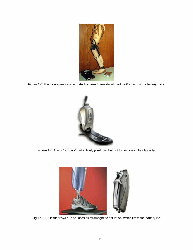
Specifically, Popovic and Schwirtlich (1988) report the development of a battery-powered active knee

joint actuated by DC motors, Figure 1-5, together with a finite state knee controller that utilizes a robust

position tracking control algorithm for gait control (Popovic et. al., 1995). With regard to powered ankle

joints, Klute et al. (1998, 2000) describe the design of an active ankle joint using pneumatic McKibben

actuators, although gait control algorithms were not described. Au et al. (2005) assessed the feasibility of

an EMG based position control approach for a transtibial prosthesis. Finally, though no published

literature exists, Ossur, a major prosthetics company based in Iceland, has announced the development of

both a powered knee and a self-adjusting ankle. The latter, called the “Proprio Foot” (Figure 1-6) is not a

true powered ankle, since it does not contribute power to gait, but rather is used to quasistatically adjust

the angle of the ankle to better accommodate sitting and slopes. The powered knee, called the “Power

Knee” (Figure 1-7), utilizes an echo control approach similar to the one described by Grimes et al. (1977).

5

Figure 1-5. Electromagnetically actuated powered knee developed by Popovic with a battery pack.

Figure 1-6. Ossur "Proprio" foot actively positions the foot for increased functionality.

Figure 1-7. Ossur "Power Knee" uses electromagnetic actuation, which limits the battery life.

6

3. Motivation and Contribution

One of the most significant challenges in the development of a powered lower limb prosthesis is

providing self-powered actuation capabilities comparable to biological systems. State-of-the-art power

supply and actuation technology such as battery/DC motor combinations suffer from low energy density of

the power source (i.e., heavy batteries for a given amount of energy), low actuator force/torque density,

and low actuator power density (i.e., heavy motor/gearhead packages for a given amount of force or

torque and power output), all relative to the human musculoskeletal system. Recent advances in power

supply and actuation for self-powered robots, such as the liquid-fueled approaches described by Goldfarb

et al. 2003, Shields et al. 2006, Fite et al. 2006, and Fite and Goldfarb 2006, offer the potential of

significantly improved energetic characteristics relative to battery/DC motor combinations, and thus bring

the potential of a powered lower limb prosthesis to the near horizon. Specifically, the aforementioned

publications describe pneumatic-type actuators, which are powered by the reaction products of a

catalytically decomposed liquid monopropellant. The proposed approach has been experimentally

shown to provide an energetic figure of merit an order of magnitude greater than state-of-the-art batteries

and motors (Shields et al. 2006, Fite and Goldfarb 2006). Based on this liquid-fueled approach, a

prototype of a powered knee and ankle transfemoral prosthesis have been developed (Sup and Goldfarb

2007).

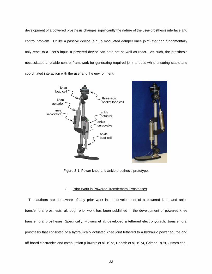
The development of a powered prosthesis changes significantly the nature of the user-prosthesis

interface and control problem. Unlike a passive device (e.g., a modulated damper knee joint) that can

fundamentally only react to a user’s input, a powered device can both act as well as react. As such, the

prosthesis necessitates a reliable control framework for generating required joint torques while ensuring

7

stable and coordinated interaction with the user and the environment. This thesis proposes an intelligent

control framework for the control of the powered knee and ankle transfemoral prosthesis.

4. Organization of the Document

The thesis is organized into four chapters. The references for each chapter is given at the end of the

chapter. Chapter I presents the introduction and motivation for the intelligent control of a powered

transfemoral prosthesis. Chapter II is a conference paper that is published in the Proceedings of the 10th

International Conference on Rehabilitation Robotics (ICORR 2007). The paper presents a k-Nearest

Neighbor algorithm based real-time gait intent recognition approach for use in controlling a fully powered

transfemoral prosthesis described. The proposed approach infers user intent based on the characteristic

shape of the force and moment vector of interaction between the user and prosthesis.

Chapter III is also a conference paper that is published in the Proceedings of the 10th International

Conference on Rehabilitation Robotics (ICORR 2007). This paper presents an active passive torque

decomposition procedure for use in controlling a fully powered transfemoral prosthesis. The active and

passive parts of the joint torques are extracted by solving a constrained least squares optimization problem.

The proposed approach generates the torque reference of joints by combining the active part, which is a

function of the force and moment vector of the interaction between user and prosthesis and the passive

part, which has a nonlinear spring-dashpot behavior. The last chapter, Chapter IV, describes the

experimental procedure for the calibration of the three axis socket load cell, the main component of the

mechanical sensory interface of the powered prosthesis.

8

5. References

Au, S. Bonato, P., Herr, H., “An EMG-Postion Controlled System for an Active Ankle-Foot Prothesis: An Initial Experimental Study,” Proceedings of the IEEE Int Conf. on Rehabilitation Robotics, pp. 375-379, 2005.

DeVita, P., Torry M., Glover, K.L., and Speroni, D.L.,“A Functional Knee Brace Alters Joint Torque and Power Patterns during Walking and Running,” Journal of Biomechanics, vol. 29, no. 5, pp. 583-588, 1996.

Donath, M., “Proportional EMG Control for Above-Knee Prosthesis’, Department of Mechanical Engineering Masters Thesis, MIT, 1974.

Fite, K.B., and Goldfarb, M. Design and Energetic Characterization of a Proportional-Injector Monopropellant-Powered Actuator, IEEE/ASME Transactions on Mechatronics, vol. 11, no. 2, pp. 196-204, 2006.

Fite, K.B., Mitchell, J., Barth, E.J., and Goldfarb, M. A Unified Force Controller for a Proportional-Injector Direct-Injection Monopropellant-Powered Actuator, ASME Journal of Dynamic Systems, Measurement and Control, vol. 128, no. 1, pp. 159-164, 2006.

Flowers, W.C., “A Man-Interactive Simulator System for Above-Knee Prosthetics Studies, Department of Mechanical Engineering PhD Thesis, MIT, 1973.

Flowers, W.C., and Mann, R.W., “Electrohydraulic knee-torque controller for a prosthesis simulator,” ASME Journal of Biomechanical Engineering, vol. 99, no. 4, pp. 3-8., 1977.

Goldfarb, M., Barth, E.J., Gogola, M.A. and Wehrmeyer, J.A., “Design and Energetic Characterization of a Liquid-Propellant-Powered Actuator for Self-Powered Robots.,” IEEE/ASME Transactions on Mechatronics, vol. 8, no. 2, pp. 254-262, 2003.

Grimes, D. L., “An Active Multi-Mode Above Knee Prosthesis Controller. Department of Mechanical Engineering PhD Thesis, MIT., 1979.

Grimes, D. L., Flowers, W. C., and Donath, M., “Feasibility of an active control scheme for above knee prostheses. ASME Journal of Biomechanical Engineering, vol. 99, no. 4, pp. 215-221, 1977.

Jacobs, R., Bobbert, M.F., van Ingen Schenau, G.J.; “Mechanical output from individual muscles during explosive leg extensions: the role of biarticular muscles,” Journal of Biomechanics, vol. 29, no. 4, pp. 513-523, 1996.

Klute, G.K., Czerniecki, J., Hannaford, B., “Development of Powered Prosthetic Lower Limb, Proceedings of the First National Meeting, Veterans Affairs Rehabilitation Research and Development Service, 1998.

Klute, G.K., Czerniecki, J., Hannaford, B., “Muscle-Like Pneumatic Actuators for Below-Knee Prostheses,

9

Proceedings the Seventh International Conference on New Actuators, pp. 289-292, 2000.

Nadeau, S., McFadyen, B.J., and Malouin, F., “Frontal and sagittal plane analyses of the stair climbing task in healthy adults aged over 40 years: What are the challenges compared to level walking?,” Clinical Biomechanics, vol. 18, no. 10, pp. 950-959., 2003.

Nagano, A., Ishige, Y., and Fukashiro, S., “Comparison of new approaches to estimate mechanical output of individual joints in vertical jumps,” Journal of Biomechanics, vol. 31, no. 10, pp. 951-955, 1998.

Popovic, D. and Schwirtlich, L., “Belgrade active A/K prosthesis, “ in de Vries, J. (Ed.), Electrophysiological Kinesiology, Interm. Congress Ser. No. 804, Excerpta Medica, Amsterdam, The Netherlands, pp. 337–343, 1988.

Popovic D, Oguztoreli MN, Stein RB., “Optimal control for an above-knee prosthesis with two degrees of freedom,” Journal of Biomechanics, vol. 28, no. 1, pp. 89-98, 1995.

Prilutsky, B.I., Petrova, L.N., and Raitsin, L.M., “Comparison of mechanical energy expenditure of joint moments and muscle forces during human locomotion,” Journal of Biomechanics, vol. 29, no. 4, pp. 405-415, 1996.

Riener, R., Rabuffetti, M., and Frigo, C., “Joint powers in stair climbing at different slopes.”, Proceedings of the IEEE International Conference on Engineering in Medicine and Biology, vol. 1, p. 530., 1999.

Shields, B.L., Fite, K., and Goldfarb, M. Design, Control, and Energetic Characterization of a Solenoid Injected Monopropellant Powered Actuator, IEEE/ASME Transactions on Mechatronics, vol. 11, no. 4, pp. 477-487, 2006.

Stein, J.L., “Design Issues in the Stance Phase Control of Above-Knee Prostheses,” Department of Mechanical Engineering PhD Thesis, MIT, 1983.

Stein, J.L., and Flowers, W.C., “Stance phase control of above-knee prostheses: knee control versus SACH foot design,” Journal of Biomechanics, vol. 20, no. 1, pp. 19-28, 1988.

Sup, F., Amit, B., and Goldfarb M., "Design and Control of a Powered Knee and Ankle Prosthesis," Proceedings of the 2007 IEEE International Conference on Robotics and Automation, pp. 4134-4139.

Waters, R., Perry, J., Antonelli, D., and Hislop, H., “Energy cost of walking amputees: the influence of level of amputation,” J. Bone and Joint Surgery. 58A, 42–46, 1976.

Winter, D. A. and Sienko, S. E., “Biomechanics of below-knee amputee gait,” J. Biomechanics. 21, 361–367., 1988.

Winter, D.A., “The biomechanics and motor control of human gait: normal, elderly and pathological,” University of Waterloo Press, 2nd ed., 1991.

10

CHAPTER II

MANUSCRIPT I: REAL-TIME INTENT RECOGNITION FOR A POWERED KNEE AND ANKLE TRANSFEMORAL PROSTHESIS

Huseyin Atakan Varol and Michael Goldfarb

Department of Mechanical Engineering

Vanderbilt University

Nashville, TN 37235

ICORR 2007 10th International Conference on Rehabilitation Robotics

June 13-15, 2007, Noordwijk, Netherlands

11

1. Abstract

This paper describes a real-time gait intent recognition approach for use in controlling a fully powered

transfemoral prosthesis. Rather than utilize an “echo control” approach as proposed by others, which

requires instrumentation of the sound-side leg, the proposed approach infers user intent based on the

characteristic shape of the force and moment vector of interaction between the user and prosthesis. The

real-time intent recognition approach utilizes a K-nearest neighbor algorithm with majority voting and

threshold biasing schemes to increase its robustness. The ability of the approach to recognize in real time

a person’s intent to stand or walk at one of three different speeds is demonstrated on measured

biomechanics data.

2. Introduction

Despite significant technological advances over the past decade, such as the introduction of

microcomputer-modulated damping during swing, commercial transfemoral prostheses remain essentially

limited to energetically passive devices. That is, the joints of the prostheses can either store or dissipate

energy, but cannot provide net power over a gait cycle. The knee and ankle joints of the native limb,

however, generate significant net power output over a gait cycle during many locomotive functions,

including walking upstairs and up slopes, running, and jumping (Winter and Sienko 1988, Nadeau et al.

2003, Riener et al. 1999, Prilutsky et al. 1996, DeVita et al. 1996, Nagano et al. 1998, Jacobs et al. 1996) .

Even during level walking, transfemoral amputees with passive prostheses exhibit asymmetric gait

kinematics, expend up to 60% more metabolic energy relative to healthy subjects (Walters et al. 1976),

and exert as much as three times the affected-side hip power and torque relative to healthy subjects, all of

12

which are indicative of the functional limitations of passive joints (Winter 1991).

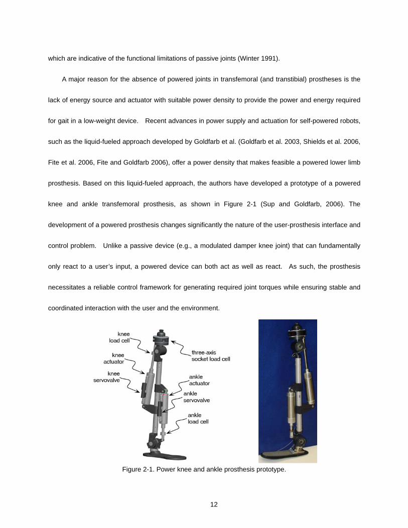
A major reason for the absence of powered joints in transfemoral (and transtibial) prostheses is the

lack of energy source and actuator with suitable power density to provide the power and energy required

for gait in a low-weight device. Recent advances in power supply and actuation for self-powered robots,

such as the liquid-fueled approach developed by Goldfarb et al. (Goldfarb et al. 2003, Shields et al. 2006,

Fite et al. 2006, Fite and Goldfarb 2006), offer a power density that makes feasible a powered lower limb

prosthesis. Based on this liquid-fueled approach, the authors have developed a prototype of a powered

knee and ankle transfemoral prosthesis, as shown in Figure 2-1 (Sup and Goldfarb, 2006). The

development of a powered prosthesis changes significantly the nature of the user-prosthesis interface and

control problem. Unlike a passive device (e.g., a modulated damper knee joint) that can fundamentally

only react to a user’s input, a powered device can both act as well as react. As such, the prosthesis

necessitates a reliable control framework for generating required joint torques while ensuring stable and

coordinated interaction with the user and the environment.

Figure 2-1. Power knee and ankle prosthesis prototype.

13

3. Prior Work in Powered Transfemoral Prosthesis

The authors are not aware of any prior work in the development of a powered knee and ankle

transfemoral prosthesis, although prior work has been published in the development of powered knee

transfemoral prostheses. Specifically, Flowers et al. developed a tethered electrohydraulic transfemoral

prosthesis that consisted of a hydraulically actuated knee joint tethered to a hydraulic power source and

off-board electronics and computation (Flowers et al. 1973, Donath et al. 1974, Grimes et al. 1979, Grimes

et al. 1977, Stein et al. 1983, Flowers et al. 1977). They subsequently developed an “echo control” scheme

for gait control, as described by Grimes et al. (1977), in which a modified knee trajectory from the sound

leg is played back on the contralateral side. Popovic and Schwirtlich (1988) report the development of a

battery-powered active knee joint actuated by DC motors, together with a finite state knee controller that

utilizes robust position tracking control algorithm for gait control. Finally, Ossur, a major prosthetics

company based in Iceland, has announced the limited launch of a powered knee, called the “Power Knee,”

which purportedly uses sensors on the sound side leg as input for the control of the powered prosthesis.

4. Interface Approaches

Unlike existing passive prostheses (including microprocessor-controlled devices), the introduction of

power into a prosthesis provides the ability for the device to act, rather than simply react. As such, the

development of a suitable controller that provides for stable and reliable interaction between the user and

prosthesis is paramount. The user interface and control issue can be addressed with widely varying

approaches and at widely varying degrees of invasiveness. The major categories of interface, in order of

increasing invasiveness, are (1) mechanical sensory interface, (2) surface electromyography (EMG)

14

interface, (3) implantable peripheral nervous systems (PNS) interface, and (4) implantable central nervous

system (CNS) interface. Mechanical sensory interface (MSI) approaches use only sensors pertaining to

the biomechanics of gait (i.e., as opposed to the physiology of gait), such as measurement of forces,

torques, joint angles, and vertical orientation (i.e., inclination). Surface EMG, which is the approach used

by actively powered myoelectric upper extremity prostheses, incorporates surface electrodes (often in the

prosthesis socket) to extract command signals from the muscles in the residual limb. Some researchers

have investigated the use of surface EMG control approaches for knee control in a lower limb prostheses,

including (Aeyels et al. 1995, Donath 1974, Myers and Moskowitz 1981, Myers and Moskowitz 1983, Triolo

and Moskowitz 1982, Aeyels et al. 1992, Peeraer et al. 1990). In the case of an upper extremity

above-elbow myoelectric prosthesis, the combination of the biceps and triceps EMG provides a single

bipolar signal, which is switched between the control of the terminal device and control of the elbow (i.e.,

does not enable simultaneous control of both joints). This approach would not be appropriate for an active

knee and ankle joint leg, however, since locomotion requires simultaneous control of the knee and ankle.

As such, an EMG approach would require at least two control channels (i.e., measurement from two sets

of antagonist muscles). Implantable PNS approaches include the use of percutaneous electrodes

implanted in the nerves, and/or the use of implantable capsules for extraction of the EMG signals, from

which neural or EMG commands can be extracted. Finally, implantable CNS approaches utilize electrode

arrays implanted in the cortex of the brain, from which motor commands can also be extracted.

Presumably, the extent of control over the prosthesis would vary roughly inversely with the extent of

invasiveness.

As with any medical device or procedure, one would optimally wish to incorporate the least invasive

15

approach that achieves the desired specific aims, and as such, the proposed controller utilizes the

non-invasive mechanical sensory interface approach. The lower limb, in particular, lends itself much more

readily to non-invasive interface approaches than does the upper limb, since (1) the lower limb

fundamentally interacts mechanically with the environment (i.e., the ground and the user) and (2) the tasks

in which the lower limb engages are typically periodic in nature. Both of these qualities are leveraged in the

proposed design.

Although the commercially available passive computer controlled knee systems (e.g., C-leg, Rheo

knee) already make use of signals only taken from the instrumented prosthesis for real-time mode

detection and subsequent knee control, the previously cited works on powered knees all incorporate a

variation of echo control, in which the sound-side (i.e., unaffected) leg is instrumented to provide input

commands for the powered prosthesis. The obvious drawback to such an approach is that the sound-side

(or unaffected) leg must be instrumented, which requires the user to don and doff additional equipment

and associated wiring. The echo control approach also restricts the use of the prosthesis to unilateral

amputees and also presents a problem for “odd” numbers of steps, in which an echoed step is undesirable.

A more subtle, although perhaps more significant shortcoming of the echo-type approach is that suitable

motion tracking requires a high output impedance of the prosthesis, which forces the amputee to react to

the limb rather than interact with it. Specifically, in order for the prosthesis to dictate the joint trajectory, it

must assume a high output impedance (i.e., must be stiff), thus precluding any dynamic interaction with the

user and the environment, which is in turn contrary to the way in which humans interact with their native

limbs.

This paper offers an alternative approach to addressing the interface between user and prosthesis

16

that is both non-invasive and obviates the need for sound-side instrumentation. Rather than gather user

intent from the joint angle measurements from the contralateral unaffected leg, the proposed approach

infers commands from the user via the (ipsilateral) forces and moments of interaction between the user

and prosthesis. Specifically, the user interacts with the prosthesis by imparting forces and moments from

the residual limb to the prosthesis, all of which can be measured via a multi-axis load cell. These forces

and moments serve not only as a means of physical interaction, but also serve as an implicit

communication channel between the user and device, with the user’s intent encoded in this measurement.

Inferring user’s intent from the measured forces and moments of interaction provides several advantages

relative to the echo approach. First, no instrumentation or wiring apart from the prosthesis need be worn

by the user. Second, unlike an echo approach, the information flow is immediate (i.e., the user intent

need not be delayed by a half cycle). Third, the prosthesis command is decoupled from the unaffected

side, and thus the user is not constrained to “even” patterns of gait. Finally, unlike an echo approach, the

proposed approach can be utilized on either a unilateral or bilateral amputee.

This paper describes a method for the real-time recognition of user intent based primarily on the

forces and moments of interaction between the user and prosthesis, and demonstrates on biomechanical

data that the proposed approach can differentiate between standing and three different walking speeds.

5. K-Nearest Neighbor Classification

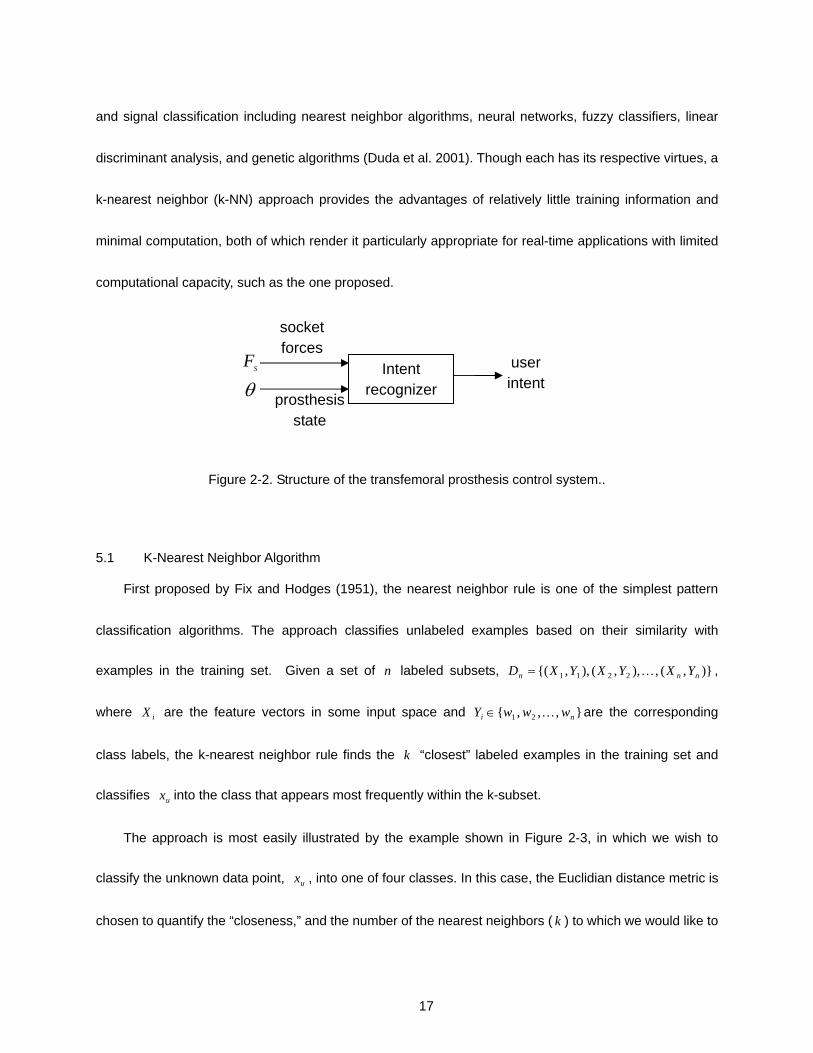
Gait intent recognition is a real time pattern recognition or signal classification problem. The signal in

this case is the combination of socket interface forces and the dynamic state of the prosthesis, which is a

vector of the knee and ankle angles as illustrated in Figure 2-2. Many methods exist for pattern recognition

17

and signal classification including nearest neighbor algorithms, neural networks, fuzzy classifiers, linear

discriminant analysis, and genetic algorithms (Duda et al. 2001). Though each has its respective virtues, a

k-nearest neighbor (k-NN) approach provides the advantages of relatively little training information and

minimal computation, both of which render it particularly appropriate for real-time applications with limited

computational capacity, such as the one proposed.

Figure 2-2. Structure of the transfemoral prosthesis control system..

5.1 K-Nearest Neighbor Algorithm

First proposed by Fix and Hodges (1951), the nearest neighbor rule is one of the simplest pattern

classification algorithms. The approach classifies unlabeled examples based on their similarity with

examples in the training set. Given a set of n labeled subsets, )},(,),,(),,{( 2211 nnn YXYXYXD K= ,

where iX are the feature vectors in some input space and },,,{ 21 ni wwwY K∈ are the corresponding

class labels, the k-nearest neighbor rule finds the k “closest” labeled examples in the training set and

classifies ux into the class that appears most frequently within the k-subset.

The approach is most easily illustrated by the example shown in Figure 2-3, in which we wish to

classify the unknown data point, ux , into one of four classes. In this case, the Euclidian distance metric is

chosen to quantify the “closeness,” and the number of the nearest neighbors ( k ) to which we would like to

Intent recognizer

SF

θ

socket forces

prosthesis state

user intent

18

quantify the closeness of the data point is chosen to be five (note that the number depends on the number

of classes, number of points, nature of the classes, etc.). As depicted in the figure, three of the nearest

neighbors belong to the class 4w , while two belong to the class 1w . The data point is therefore assigned to

class 4w , since it has the most “nearest neighbors” in that class.

Figure 2-3. Illustration of the k-NN algorithm for the classification of an unknown example, ux , with 5

nearest neighbors and 4 classes.

5.2 Application of k-NN to Gait Mode Recognition

For purposes of intent recognition in a powered prosthesis, the algorithm must be fast (relative to the

step period), must be real-time (i.e., satisfaction of hard deadline constraints is needed due to the safety

critical nature of the task), must be robust to noise, and must be computationally inexpensive since it will

be implemented on an embedded computing platform with limited computational capability.

In this work, the k-NN algorithm described in the previous section is modified and enhanced to detect

the different gait modes. At this point in its development, the k-NN based intent recognizer detects four

19

different gait modes, iq , which are standing ( 1q ) and three different walking speeds (slow ( 2q ), normal ( 3q )

and fast ( 4q )). Note that in a realistic implementation, several classes would be considered, including

walking upstairs and downstairs and walking backwards. Despite this, the aforementioned set of four

classes serves as an appropriate initial set with which to develop and test the proposed approach.

At each time step of the algorithm, an unlabeled example vector consisting of the sensor

measurement vector, TanklekneeSSu FFx ],,,[

21θθ= , is classified as one of the four gait modes. The sensor

measurement consists of the socket load forces in the sagittal plane, 1SF and

2SF , and the knee and

ankle angles, kneeθ and ankleθ . At each iteration, the distance of the new unclassified sample relative to the

each class of data points is calculated. Two measures of closeness were compared, the Euclidian norm

and the absolute norm. The distance of the unclassified sample vector, ux , relative to a vector, ix , in

the training set is given for the Euclidian and absolute case respectively as:

∑=

−=4

1

2)(j

iui jjeuclidianxxc (1)

∑=

−=4

1jiui jjabs

xxc (2)

Once the k nearest neighbors are determined, the sample vector is classified as the class with the

most members of this set. In order to decrease sensitivity to noise, classification of the current sample

vector is additionally debounced and filtered. The debouncing is based on a threshold biasing scheme, in

which at each time step, the number of members of the nearest neighbor set for the predominant class in

the previous time step is multiplied by a biasing constant, 1>a . Appropriate tuning of this parameter

decreases the likelihood of switching classes, and thus inhibits chattering between classes. The output of

the classifier is additionally filtered by a boxcar window of length p. Figure 2-4 lists the psuedocode of the

20

classification algorithm.

Figure 2-4. Pseudocode of the k-NN based intent recognition algorithm.

6. Implementation and Experimental Validation

6.1 Gait Experiments

In order to validate the ability of the proposed approach to determine user intent in real-time, the

authors generated an experimental database consisting of the appropriate data vectors for various data

classes (i.e., for standing and three different walking speeds). Note that two major differences exist

between the conditions used for validation of the approach and the manner in which the approach would

eventually be implemented in a prosthesis. First, the gait data was generated by a normal subject rather

21

than from an amputee. Second, the intent recognition algorithm was tested following the collection of all

data, rather than in a real-time setting. Both variations were a matter of experimental convenience, and

neither affects significantly the validity of the results. Specifically, the use of a normal subject rather than an

amputee affects two issues. First, the mass distribution of the leg will be slightly different than if it were a

prosthesis. Second, since the vector of sagittal plane forces of interaction between the user and

prosthesis is not readily measured in a normal subject, the algorithm instead used the vector of sagittal

plane hip torque and ground reaction force, which are related to the former by a coordinate transformation.

In other words, both force vectors fundamentally contain the same information, but are simply measured in

different locations. Regarding the real-time aspect, the algorithm was required to run at a high sampling

speed (i.e., 10 msec) and to be strictly causal, and as such could have been implemented in real-time.

Due to the use of a normal subject, however, the real-time implementation was not possible, since the hip

torque could not be directly measured, but rather had to be computed via post-processing of the measured

data (as is typical in the acquisition of kinetic gait data). Note that in a transfemoral prosthesis (such as

the one shown in Figure 2-1), the force data would be measured on the prosthesis, and thus would be

available for real-time use.

In order to generate appropriate kinematic and kinetic data for definition of the data classes and for

testing of the approach, gait experiments were conducted in the Biomechanics and Sports Medicine

Laboratory of the University of Tennessee at Knoxville. The experimental setup consisted of a 7-camera

240 Hz VICON MX system and 2 AMTI multiaxis force platforms. As is standard in such a setup, hip, knee

and ankle angles were measured via the cameras, the ground reaction force was measured using the

multiaxis force plates, and the joint torques and forces were computed in post-processing via inverse

22

dynamics, based on inertial parameters estimated with lookup tables. The sampling rate for the cameras

and the force plates were 100 Hz and 1000 Hz, respectively. Data collection consisted of two 30-second

trials for standing (ST) and four trials each for standing to walking (S2W), walking to standing (W2S), slow

walking (WS), normal walking (WN) and fast walking (WF). In the standing trials, the subject was asked to

stand and shift his weight around as he normally would. For the stand to walk transition, the subject was

asked to stand on the force plate for approximately five seconds, then proceed to a normal walk at a

self-selected pace. For the walk to stand transition, the subject was asked to walk at a self-selected pace,

then as naturally as possible come to a stop on the force plate. For the slow, normal, and fast walking,

the subject was asked to walk at those respective rates, while an optical interrupt timing system measured

the walking speed between the subject’s entrance and exit of the camera viewing volume. The minimum,

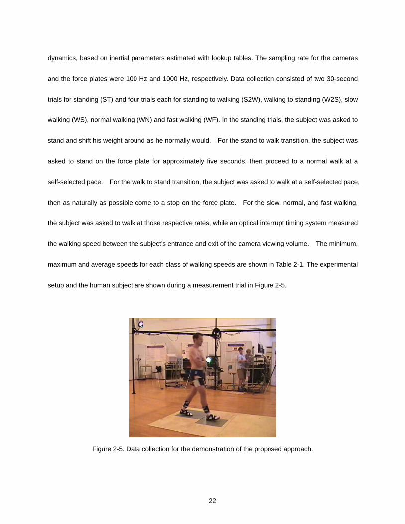
maximum and average speeds for each class of walking speeds are shown in Table 2-1. The experimental

setup and the human subject are shown during a measurement trial in Figure 2-5.

Figure 2-5. Data collection for the demonstration of the proposed approach.

23

6.2 Class Database and Generation of Test Sequences

Since kinetic data is only available during contact with the force plates, the amount of data with which

to define various classes and test the system was limited. Given the limited amount of data, all trials of

each class were concatenated to form the database defining that particular class (i.e., standing, slow

walking, normal walking, and fast walking). The “test” data was formed by assembling linear combinations

of trial data and by inserting stand to walk and walk to stand transition data between the standing and

walking data. Then the test data is smoothed with a low pass filter in order to remove the spikes occurring

due to the concenation of the datasets. Recall, that each training set contains time marked arrays of the

hip torque, the ground reaction force, knee and ankle angles, all at a sampling rate of 10 ms. The

components of each data set were additionally scale-normalized between 0 and 1 in order to make the

relative importance of all the time marked arrays equal. Note that the normalization constants obtained

from the training data will also be employed to normalize the measurement data at each sampling instant

in the real-time application. Note also that the objective of the intent recognizer is only to determine intent

for a single user, as opposed to generalized intent recognition across subjects. As such, each subject

would require a separate database defining the various classes of locomotion (i.e., a database

representing the spectrum of user intentions).

TABLE 2-1

WALKING EXPERIMENT PARAMETERS

Walking Mode

Minimum Speed (m/s)

Average Speed (m/s)

Maximum Speed (m/s)

Slow 1.01 1.04 1.07 Normal 1.19 1.22 1.26

Fast 1.45 1.51 1.56

24

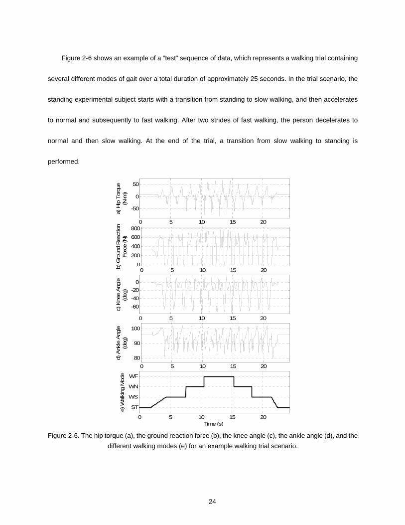
Figure 2-6 shows an example of a “test” sequence of data, which represents a walking trial containing

several different modes of gait over a total duration of approximately 25 seconds. In the trial scenario, the

standing experimental subject starts with a transition from standing to slow walking, and then accelerates

to normal and subsequently to fast walking. After two strides of fast walking, the person decelerates to

normal and then slow walking. At the end of the trial, a transition from slow walking to standing is

performed.

0 5 10 15 20

-50

0

50

a) H

ip T

orqu

e(N

-m)

0 5 10 15 200

200

400

600

800

b) G

roun

d R

eact

ion

Forc

e (N

)

0 5 10 15 20

-60-40-20

0

c) K

nee

Ang

le(d

eg)

0 5 10 15 2080

90

100

d) A

nkle

Ang

le(d

eg)

0 5 10 15 20

ST

WS

WN

WF

e) W

alki

ng M

ode

Time (s)

Figure 2-6. The hip torque (a), the ground reaction force (b), the knee angle (c), the ankle angle (d), and the different walking modes (e) for an example walking trial scenario.

25

7. Results and Discussion

The k-NN intent recognizer was implemented on a PC with an Intel Pentium 4 (2 GHz) processor with

1024MB memory using Matlab 7.0. In order to simulate real-time conditions, the algorithm was run with a

fixed time step of 10 msec. The algorithm includes three parameters which can be tuned, based on the

nature and amount of noise in the data, to result in the least mode estimation error. The three parameters

are the biasing constant, a, the number of nearest neighbors, k, and the length of the boxcar window, p.

The value of the biasing constant, a, was experimentally tuned independently of the other parameters. A

higher value of this constant makes the algorithm more robust and prevents chattering between different

modes, but, it also causes delays in the transitions which is not desirable. Figure 2-7 shows a trial

scenario depicting a transition from normal walking to fast walking. As can be seen, when the parameter

2=a , the transition is recognized in approximately 0.17 seconds, although chattering is present in the

classification. In the case that 3=a , the chattering does not occur and the delay in the recognition is

nearly the same. When 4=a , the transition delay increases substantially to 0.4 seconds. As such, the

biasing constant was set to 3=a for the work presented here, which was determined to be the best

trade-off between delay and chatter.

For the data shown in Figure 2-6, the values of the other two parameters were determined by an

exhaustive search for the smallest estimation error with integer values of the parameters 253 ≤≤ k and

322 ≤≤ p . The results of this search for both absolute and the Euclidian norms are shown in Table 2-2,

which indicates that the smallest mode identification error is obtained when the absolute norm is used and

the values of nearest neighbors, k, and the length of the boxcar window, p, are set to 7 and 16 respectively.

The results for the “best case” set of parameters are therefore 3=a , 7=k , and 16=p , with the best

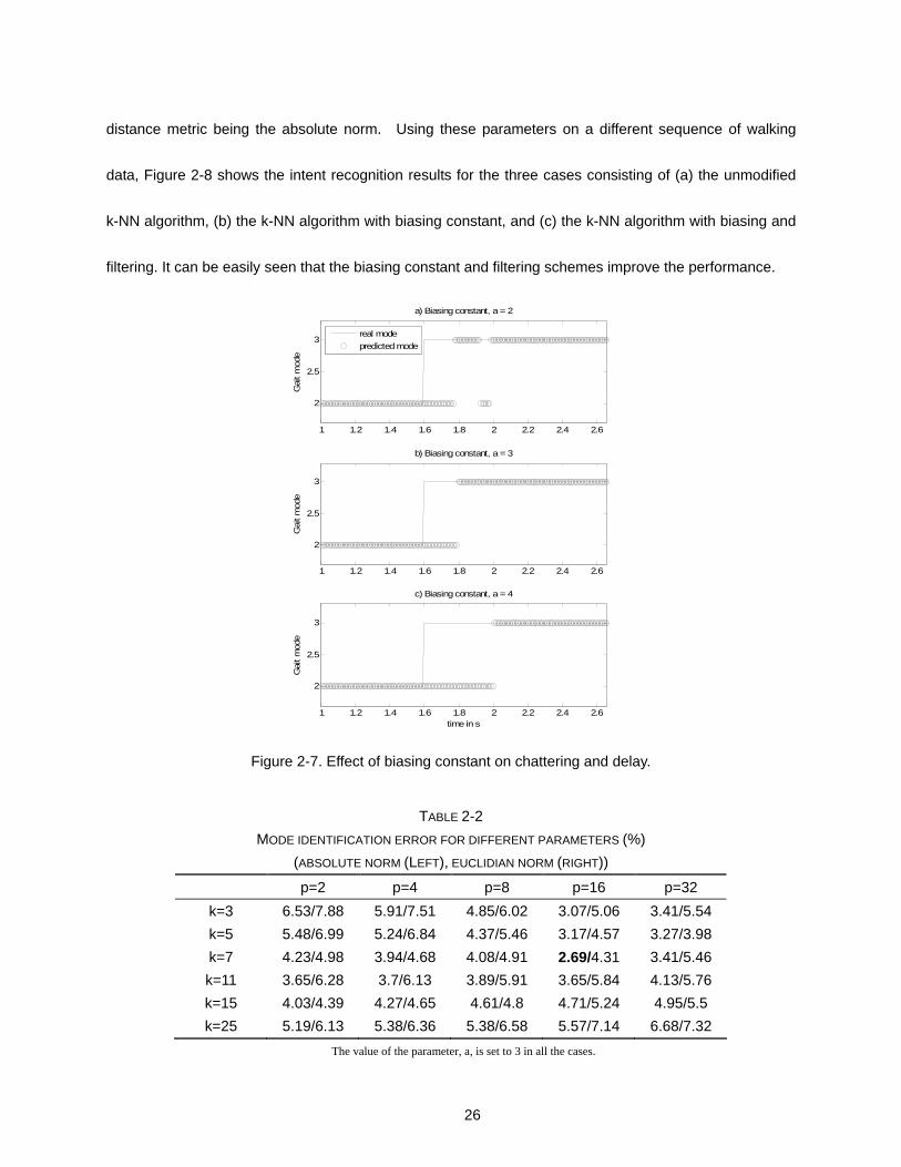
26

distance metric being the absolute norm. Using these parameters on a different sequence of walking

data, Figure 2-8 shows the intent recognition results for the three cases consisting of (a) the unmodified

k-NN algorithm, (b) the k-NN algorithm with biasing constant, and (c) the k-NN algorithm with biasing and

filtering. It can be easily seen that the biasing constant and filtering schemes improve the performance.

1 1.2 1.4 1.6 1.8 2 2.2 2.4 2.6

2

2.5

3

a) Biasing constant, a = 2

Gai

t mod

e

1 1.2 1.4 1.6 1.8 2 2.2 2.4 2.6

2

2.5

3

b) Biasing constant, a = 3

Gai

t mod

e

1 1.2 1.4 1.6 1.8 2 2.2 2.4 2.6

2

2.5

3

c) Biasing constant, a = 4

Gai

t mod

e

time in s

real modepredicted mode

Figure 2-7. Effect of biasing constant on chattering and delay.

TABLE 2-2 MODE IDENTIFICATION ERROR FOR DIFFERENT PARAMETERS (%)

(ABSOLUTE NORM (LEFT), EUCLIDIAN NORM (RIGHT))

p=2 p=4 p=8 p=16 p=32 k=3 6.53/7.88 5.91/7.51 4.85/6.02 3.07/5.06 3.41/5.54 k=5 5.48/6.99 5.24/6.84 4.37/5.46 3.17/4.57 3.27/3.98 k=7 4.23/4.98 3.94/4.68 4.08/4.91 2.69/4.31 3.41/5.46 k=11 3.65/6.28 3.7/6.13 3.89/5.91 3.65/5.84 4.13/5.76 k=15 4.03/4.39 4.27/4.65 4.61/4.8 4.71/5.24 4.95/5.5 k=25 5.19/6.13 5.38/6.36 5.38/6.58 5.57/7.14 6.68/7.32

The value of the parameter, a, is set to 3 in all the cases.

27

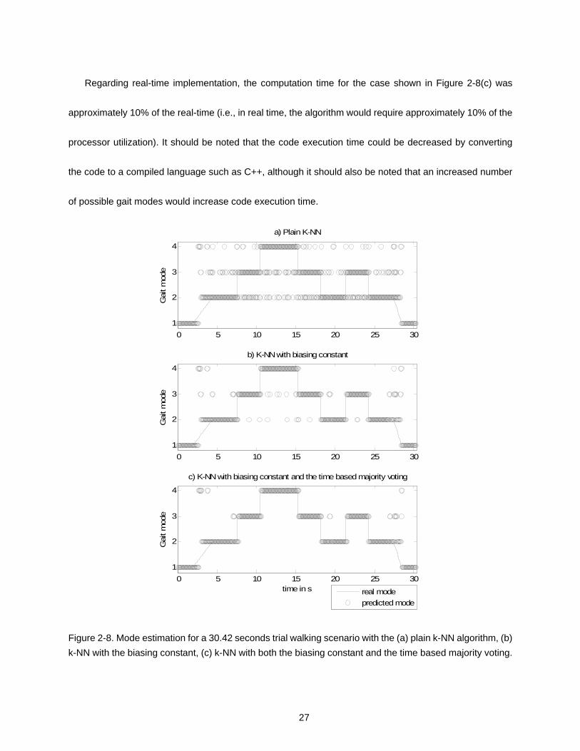
Regarding real-time implementation, the computation time for the case shown in Figure 2-8(c) was

approximately 10% of the real-time (i.e., in real time, the algorithm would require approximately 10% of the

processor utilization). It should be noted that the code execution time could be decreased by converting

the code to a compiled language such as C++, although it should also be noted that an increased number

of possible gait modes would increase code execution time.

0 5 10 15 20 25 301

2

3

4

a) Plain K-NN

Gai

t mod

e

0 5 10 15 20 25 301

2

3

4

b) K-NN with biasing constant

Gai

t mod

e

0 5 10 15 20 25 301

2

3

4

c) K-NN with biasing constant and the time based majority voting

Gai

t mod

e

time in s

real modepredicted mode

Figure 2-8. Mode estimation for a 30.42 seconds trial walking scenario with the (a) plain k-NN algorithm, (b) k-NN with the biasing constant, (c) k-NN with both the biasing constant and the time based majority voting.

28

8. Conclusion

The authors hypothesized that a user’s intent could be reliably inferred in real-time based on pattern

recognition of the measured forces and moments of interaction between the user and prosthesis. Based

on a proposed k-NN intent recognizer and biomechanical experiments designed to validate the proposed

approach, the notion of extracting in real-time user’s intent from socket interaction forces appears highly

feasible. Further work includes testing the ability to extract user intent for other gait modes, including stair

ascent/descent, slope ascent/descent, and backward walking. Further work additionally includes testing

the proposed intent recognition approach on transfemoral amputees in a real-time setting.

9. References

Aeyels, B., Peeraer, L., Vander Sloten, J., Van der Perre, G., Development of an above-knee prosthesis equipped with a microcomputer-controlled knee joint: first test results. Journal of Biomedical Engineering, Vol. 14, pp. 199-202, 1992.

Aeyels, B., Van Petegem, W., Vander Sloten, J., Van der Perre, G. and Peeraer, L., EMG-based finite state approach for a microcomputer-controlled above-knee prosthesis, Annual International Conference of the IEEE Engineering in Medicine and Biology, Proceedings of IEEE Engineering in Medicine and Biology, 1995.

DeVita, P., Torry M., Glover, K.L., and Speroni, D.L. A Functional Knee Brace Alters Joint Torque and Power Patterns during Walking and Running, Journal of Biomechanics, vol. 29, no. 5, pp. 583-588, 1996.

Donath, M., Proportional EMG Control for Above-Knee Prosthesis’, Department of Mechanical Engineering Masters Thesis, MIT, 1974.

Duda, R.O, Hart, P.E., and Stork, D.G., Pattern Classification, 2nd ed., John Wiley and Sons, 2001.

Fite, K.B., Mitchell, J., Barth, E.J., and Goldfarb, M. A Unified Force Controller for a Proportional-Injector Direct-Injection Monopropellant-Powered Actuator, ASME Journal of Dynamic Systems, Measurement and Control, vol. 128, no. 1, pp. 159-164, 2006.

Fite, K.B., and Goldfarb, M. Design and Energetic Characterization of a Proportional-Injector

29

Monopropellant-Powered Actuator, IEEE/ASME Transactions on Mechatronics, vol. 11, no. 2, pp. 196-204, 2006.

Fix, E. and Hodges, J. Discriminatory analysis, nonparametric discrimination: consistency properties, USAF School of Aviation Medicine, Randolph Field, Texas, Tech. Report 4, 1951.

Flowers, W.C., A Man-Interactive Simulator System for Above-Knee Prosthetics Studies, Department of Mechanical Engineering PhD Thesis, MIT, 1973.

Flowers, W.C., and Mann, R.W. Electrohydraulic knee-torque controller for a prosthesis simulator. ASME Journal of Biomechanical Engineering, vol. 99, no. 4, pp. 3-8, 1977.

Goldfarb, M., Barth, E.J., Gogola, M.A., and Wehrmeyer, J.A.. Design and Energetic Characterization of a Liquid-Propellant-Powered Actuator for Self-Powered Robots, IEEE/ASME Transactions on Mechatronics, vol. 8, no. 2, pp. 254-262, 2003.

Grimes, D. L. An Active Multi-Mode Above Knee Prosthesis Controller. Department of Mechanical Engineering PhD Thesis, MIT, 1979.

Grimes, D. L., Flowers, W. C., and Donath, M. Feasibility of an active control scheme for above knee prostheses. ASME Journal of Biomechanical Engineering, vol. 99, no. 4, pp. 215-221, 1977.

Jacobs, R., Bobbert, M.F., van Ingen Schenau, G.J. Mechanical output from individual muscles during explosive leg extensions: the role of biarticular muscles. Journal of Biomechanics, vol. 29, no. 4, pp. 513-523, 1996.

Myers, D. and Moskowitz, G., Myoelectric pattern recognition for use in the volitional control of above-knee prosthesis, IEEE Trans. Syst. Man Cybern., Vol. SMC-11 No. 4, pp. 296-302, 1981.

Myers, D. and Moskowitz, G., Active EMG-controlled A/K prosthesis. Control aspects of prosthetics and orthotics, Proceedings of the IFAC Symposium, Columbus, OH, 1983.

Nadeau, S., McFadyen, B.J., and Malouin, F. Frontal and sagittal plane analyses of the stair climbing task in healthy adults aged over 40 years: What are the challenges compared to level walking? Clinical Biomechanics, vol. 18, no. 10, pp. 950-959, 2003.

Nagano, A., Ishige, Y., and Fukashiro, S. Comparison of new approaches to estimate mechanical output of individual joints in vertical jumps. Journal of Biomechanics, vol. 31, no. 10, pp. 951-955, 1998.

Peeraer L, Aeyels B, Van der Perre G. Development of EMG-based mode and intent recognition algorithms for a computer controlled above-knee prosthesis. J. Biomed. Eng. 1990, Vol 12, 178-182.

Popovic, D. and Schwirtlich, L. Belgrade active A/K prosthesis, in de Vries, J. (Ed.), Electrophysiological Kinesiology, Intern. Congress Ser. No. 804, Excerpta Medica, Amsterdam, The Netherlands, pp.

30

337–343, 1988.

Prilutsky, B.I., Petrova, L.N., and Raitsin, L.M. Comparison of mechanical energy expenditure of joint moments and muscle forces during human locomotion. Journal of Biomechanics, vol. 29, no. 4, pp. 405-415, 1996.

Riener, R., Rabuffetti, M., and Frigo, C. Joint powers in stair climbing at different slopes. Proceedings of the IEEE International Conference on Engineering in Medicine and Biology, vol. 1, p. 530, 1999.

Shields, B.L., Fite, K., and Goldfarb, M. Design, Control, and Energetic Characterization of a Solenoid Injected Monopropellant Powered Actuator, IEEE/ASME Transactions on Mechatronics, vol. 11, no. 4, pp. 477-487, 2006.

Stein, J.L. Design Issues in the Stance Phase Control of Above-Knee Prostheses. Department of Mechanical Engineering PhD Thesis, MIT, 1983

Stein, J.L., and Flowers, W.C. Stance phase control of above-knee prostheses: knee control versus SACH foot design. Journal of Biomechanics, vol. 20, no. 1, pp. 19-28, 1987.

Sup, F., and Goldfarb, M. Design of a Pneumatically Actuated Transfemoral Prosthesis. Proceedings of ASME International Mechanical Engineering Conference and Exposition, IMECE2006-15707, 2006.

Triolo, R. and Moskowitz, G., Autoregressive EMG analysis and prosthetic control, Proceedings of the 35th Annual Conference on Engineering in Medicine and Biology, Philadelphia, PA, 1982.

Waters, R., Perry, J., Antonelli, D., and Hislop, H. Energy cost of walking amputees: the influence of level of amputation. J. Bone and Joint Surgery. 58A, 42–46, 1976.

Winter, D.A. The biomechanics and motor control of human gait: normal, elderly and pathological, University of Waterloo Press, 2nd ed, 1991.

Winter, D. A. and Sienko, S. E. Biomechanics of below-knee amputee gait. J. Biomech . 21, 361–367, 1988.

31

CHAPTER III

MANUSCRIPT II: DECOMPOSITION-BASED CONTROL FOR A POWERED KNEE AND ANKLE TRANSFEMORAL PROSTHESIS

Huseyin Atakan Varol and Michael Goldfarb

Department of Mechanical Engineering

Vanderbilt University

Nashville, TN 37235

ICORR 2007 10th International Conference on Rehabilitation Robotics

June 13-15, 2007, Noordwijk, Netherlands

32

1. Abstract

This paper describes an active passive torque decomposition procedure for use in controlling a fully

powered transfemoral prosthesis. The active and passive parts of the joint torques are extracted by solving

a constrained least squares optimization problem. Rather than utilize "echo control" as proposed by

others, the proposed approach generates the torque reference of joints by combining the active part, which

is a function of the force and moment vector of the interaction between user and prosthesis and the

passive part, which has a nonlinear spring-dashpot behavior. The ability of the approach to reconstruct

the required joint torques is demonstrated in simulation on measured biomechanics data.

2. Introduction

Despite significant technological advances over the past decade, commercial transfemoral prostheses

remain essentially limited to energetically passive devices. The knee and ankle joints of the native limb,

however, generate significant net power output over a gait cycle during many locomotive functions,

including walking upstairs and up slopes, running, and jumping (Winter and Sienko 1988, Nadeau et al.

2003, Riener et al. 1999, Prilutsky et al. 1996, DeVita et al. 1996, Nagano et al. 1998, Jacobs et al. 1996).

A major reason for the absence of powered joints in transfemoral (and transtibial) prostheses is the lack

of energy source and actuator with suitable power density to provide the power and energy required for gait

in a low-weight device. Recent advances in power supply and actuation for self-powered robots, such as

the liquid-fueled approach developed by Goldfarb et al. (Goldfarb et al. 2003, Shields et al. 2006, Fite et al.

2006, Fite and Goldfarb 2006), offer a power density that makes a powered lower limb prosthesis feasible.

Based on this liquid-fueled approach, the authors have developed a prototype of a powered knee and ankle

transfemoral prosthesis, as described in Sup and Goldfarb (2007) and shown in Figure 3-1. The

33

development of a powered prosthesis changes significantly the nature of the user-prosthesis interface and

control problem. Unlike a passive device (e.g., a modulated damper knee joint) that can fundamentally

only react to a user’s input, a powered device can both act as well as react. As such, the prosthesis

necessitates a reliable control framework for generating required joint torques while ensuring stable and

coordinated interaction with the user and the environment.

Figure 3-1. Power knee and ankle prosthesis prototype.

3. Prior Work in Powered Transfemoral Prostheses

The authors are not aware of any prior work in the development of a powered knee and ankle

transfemoral prosthesis, although prior work has been published in the development of powered knee

transfemoral prostheses. Specifically, Flowers et al. developed a tethered electrohydraulic transfemoral

prosthesis that consisted of a hydraulically actuated knee joint tethered to a hydraulic power source and

off-board electronics and computation (Flowers et al. 1973, Donath et al. 1974, Grimes 1979, Grimes et al.

34

1977, Stein et al. 1983, Flowers et al. 1977). They subsequently developed an “echo control” scheme for

gait control, as described by Grimes et al. (1977), in which a modified knee trajectory from the sound leg is

played back on the contralateral side. Popovic and Schwirtlich (1988) report the development of a

battery-powered active knee joint actuated by DC motors, together with a finite state knee controller that

utilizes robust position tracking control algorithm for gait control. Finally, Ossur, a major prosthetics

company based in Iceland, has announced the limited launch of a powered knee, called the “Power

Knee”.

4. Interface Approaches

Unlike existing passive prostheses (including microprocessor-controlled devices), the introduction of

power into a prosthesis provides the ability for the device to act, rather than simply react. As such, the

development of a suitable controller that provides for stable and reliable interaction between the user and

prosthesis is paramount. The user interface and control issue can be addressed with widely varying

approaches and at widely varying degrees of invasiveness. The major categories of interface, in order of

increasing invasiveness, are (1) mechanical sensory interface, (2) surface electromyography (EMG)

interface, (3) implantable peripheral nervous systems (PNS) interface, and (4) implantable central nervous

system (CNS) interface. Mechanical sensory interface (MSI) approaches use only sensors pertaining to

the biomechanics of gait (i.e., as opposed to the physiology of gait), such as measurement of forces,

torques, joint angles, and vertical orientation (i.e., inclination). Surface EMG, which is the approach used

by actively powered myoelectric upper extremity prostheses, incorporates surface electrodes (often in the

prosthesis socket) to extract command signals from the muscles in the residual limb. Some researchers

35

have investigated the use of surface EMG control approaches for knee control in a lower limb prosthesis

(Aeyels et al. 1995, Donath 1974, Myers and Moskowitz 1981, Myers and Moskowitz 1983, Triolo and

Moskowitz 1982, Aeyels et al. 1992, Peeraer et al. 1990). In the case of an upper extremity above-elbow

myoelectric prosthesis, the combination of the biceps and triceps EMG provides a single bipolar signal,

which is switched between the control of the terminal device and control of the elbow (i.e., does not enable

simultaneous control of both joints). This approach would not be appropriate for an active knee and ankle

joint leg, however, since locomotion requires simultaneous control of the knee and ankle. As such, an EMG

approach would require at least two control channels (i.e., measurement from two sets of antagonist

muscles). Implantable PNS approaches include the use of percutaneous electrodes implanted in the

nerves, and/or the use of implantable capsules for extraction of the EMG signals, from which neural or

EMG commands can be extracted. Finally, implantable CNS approaches utilize electrode arrays implanted

in the cortex of the brain, from which motor commands can also be extracted. Presumably, the extent of

control over the prosthesis would vary roughly inversely with the extent of invasiveness.

As with any medical device or procedure, one would optimally wish to incorporate the least invasive

approach that achieves the desired specific aims, and as such, the proposed controller utilizes the

non-invasive mechanical sensory interface approach. The lower limb, in particular, lends itself much more

readily to non-invasive interface approaches than does the upper limb, since (1) the lower limb

fundamentally interacts mechanically with the environment (i.e., the ground and the user) and (2) the tasks

in which the lower limb engages are typically periodic in nature. Both of these qualities are leveraged in the

proposed design.

The previously cited works on powered knees all incorporate a variation of echo control, in which the

36

sound-side (i.e., unaffected) leg is instrumented to provide position commands (delayed by one half cycle)

for the powered prosthesis. The obvious drawback to such an approach is that the sound-side (or

unaffected) leg must be instrumented, which requires the user to don and doff additional equipment and

associated wiring. The echo control approach also restricts the use of the prosthesis to unilateral

amputees and also presents a problem for “odd” numbers of steps, in which an echoed step is undesirable.

A more subtle, although perhaps more significant shortcoming of the echo-type approach is that suitable

motion tracking requires a high output impedance of the prosthesis, which forces the amputee to react to

the limb rather than interact with it. Specifically, in order for the prosthesis to dictate the joint trajectory, it

must assume a high output impedance (i.e., must be stiff), thus precluding any dynamic interaction with the

user and the environment, which is in turn contrary to the way in which humans interact with their native

limbs.

5. Decomposition-Based Control

This work offers an alternative control which employs the non-invasive MSI approach and obviates the

need for sound side instrumentation. Figure 3-2 shows the structure of the proposed control system for the

powered prosthesis. In the figure, the feedback loop for each joint incorporates the open loop joint

dynamics and the decomposed passive impedance behavior, specified by the function ),( θθτ &pp f= . The

input to the feedback loop is an active torque component, which is a function of the user input measured by

the socket load cell and specified by the function )( Saa Ff=τ .

37

Figure 3-2. Structure of the transfemoral prosthesis control system.

One of the most significant aspects of the proposed controller is the inherent passivity of its structure.

Specifically, because the behavior of the leg is decomposed into an active portion that is superimposed

upon an underlying passive impedance, and because the active component is a function solely of the

user’s input, the overall device behavior is guaranteed to be passive. As shown in Figure 3-2, since the

function )θ(θ &,pf represents a passive mapping from θ and θ& to pτ (by definition of the mapping), and

since the natural leg dynamics from τ to θ and θ& are also passive, passivity theory guarantees that

the closed-loop formed by these two mappings is also passive (Slotine 1991). As such, the closed-loop

portion of the device simply reacts to the user’s input, much the way a state-of-the-art passive prosthesis

does. The only non-passive (i.e., active) portion of the controller is the component of torque directly

resulting from the user’s input (i.e., from the socket interaction forces), over which the user has

instantaneous and direct control The proposed controller therefore creates a highly stable device over

which the human has complete and reliable control. Alternatively stated, because of the structure of the

proposed controller, the prosthesis simply reacts to what the user does to it, and as such will form a natural

extension of the user.

38

In the remaining part of the paper, the active passive decomposition method will be explained and the

joint torque reference generation procedure is presented. Finally, simulation results based on measured

biomechanical data validate the effectiveness of the proposed approach.

6. Active Passive Torque Decomposition

Passive joint torque, pτ , is defined as the part of the joint torque,τ , which can be represented using

spring and dashpot constitutional relationships (passive impedance behavior). The system can only store

or dissipate energy due to this component. The active part can be interpreted as the part which supplies

energy to the system and the active joint torque is defined as pa τττ −= . This active part will be

represented as an algebraic function of the user input via the MSI (i.e socket interface forces and torques).

Gait can be considered a mainly periodic phenomena with the periods corresponding to the strides.

Hence, the decomposition of a stride will give the required active and passive torque mappings for a

specific gait mode. In general, the joint behavior exhibits varying active and passive behavior in each stride.

Therefore, segmenting of the stride in several parts is necessary. In this case, decomposition of the torque

over the entire stride period requires the decomposition of the different segments and piecewise

reconstruction of the entire segment period. In order to maintain passive behavior, however, the segments

cannot be divided arbitrarily, but rather can only be segmented when the stored energy in the passive

elastic element is zero. This requires that the phase space can only be segmented when the joint angle

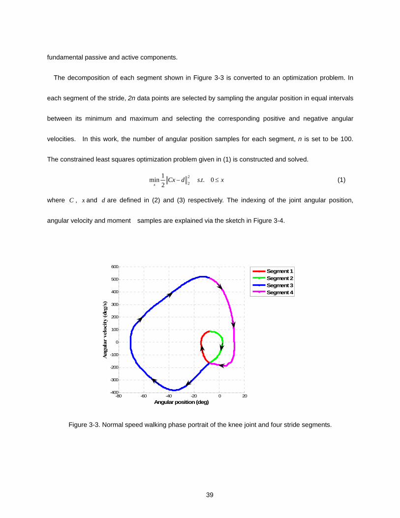
begins and ends at the same value. Figure 3-3 shows the phase portrait of normal speed walking and the

four different stride segments, 321 ,, SSS and 4S . Thus, the entire decomposition process consists of first

appropriate segmentation of the joint behavior, followed by the decomposition of each segment into its

39

fundamental passive and active components.

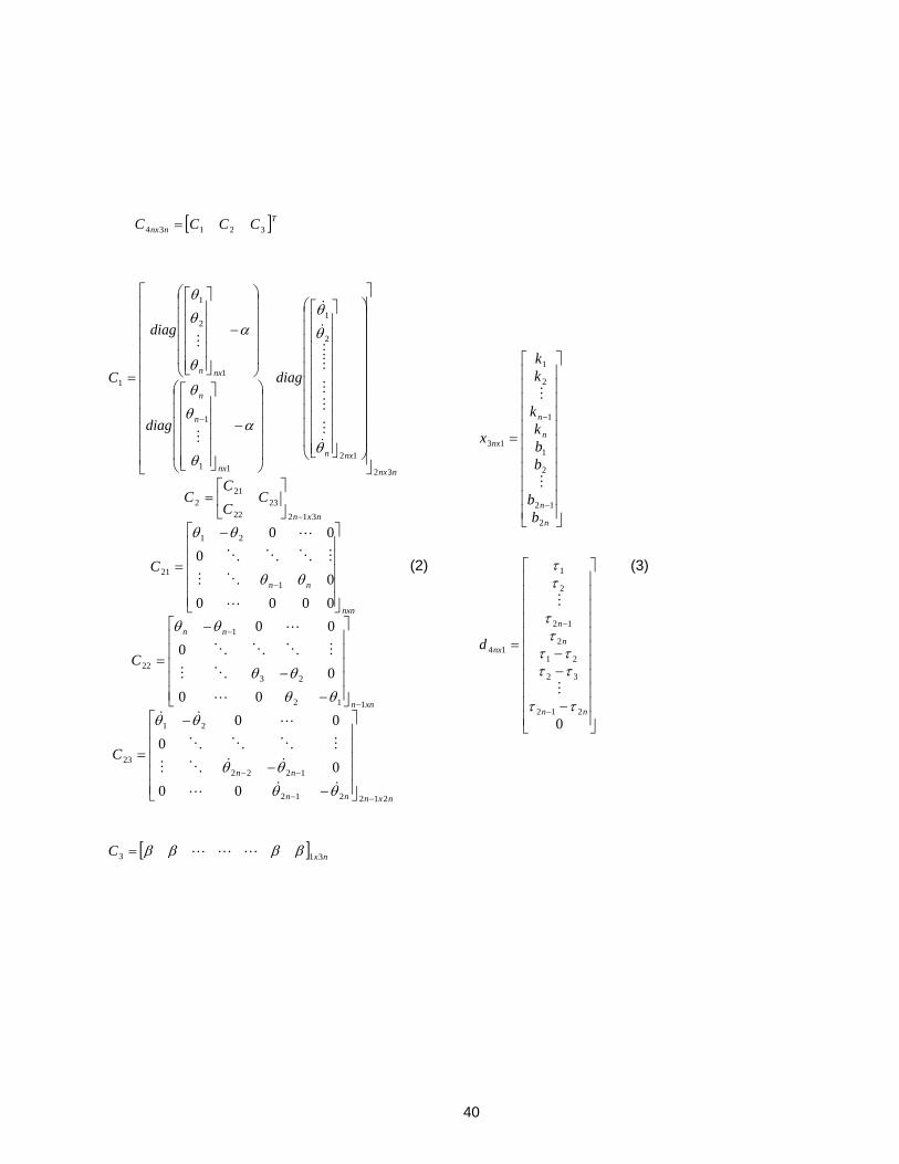
The decomposition of each segment shown in Figure 3-3 is converted to an optimization problem. In

each segment of the stride, 2n data points are selected by sampling the angular position in equal intervals

between its minimum and maximum and selecting the corresponding positive and negative angular

velocities. In this work, the number of angular position samples for each segment, n is set to be 100.

The constrained least squares optimization problem given in (1) is constructed and solved.

xtsdCxx

≤− 0..21min 2

2 (1)

where C , x and d are defined in (2) and (3) respectively. The indexing of the joint angular position,

angular velocity and moment samples are explained via the sketch in Figure 3-4.

-80 -60 -40 -20 0 20-400

-300

-200

-100

0

100

200

300

400

500

600

Angular position (deg)

Ang

ular

vel

ocity

(deg

/s)

Segment 1Segment 2Segment 3Segment 4

Figure 3-3. Normal speed walking phase portrait of the knee joint and four stride segments.

40

[ ]Tnnx CCCC 32134 =

nxnnn

nn

xnn

nn

nxn

nn

nxn

nnx

nxn

nx

n

n

nxn

C

C

C

CCC

C

diag

diag

diag

C

212212

1222

21

23

112

23

1

22

1

21

21

31223

22

212

32

12

2

1

11

1

1

2

1

1

000

000

000

00000000

000

−−

−−

−

−

−

−

−

⎥⎥⎥⎥⎥

⎦

⎤

⎢⎢⎢⎢⎢

⎣

⎡

−

−

−

=

⎥⎥⎥⎥⎥

⎦

⎤

⎢⎢⎢⎢⎢

⎣

⎡

−

−

−

=

⎥⎥⎥⎥⎥

⎦

⎤

⎢⎢⎢⎢⎢

⎣

⎡ −

=

⎥⎦

⎤⎢⎣

⎡=

⎥⎥⎥⎥⎥⎥⎥⎥⎥⎥⎥⎥

⎦

⎤

⎢⎢⎢⎢⎢⎢⎢⎢⎢⎢⎢⎢

⎣

⎡

⎟⎟⎟⎟⎟⎟⎟⎟⎟⎟

⎠

⎞

⎜⎜⎜⎜⎜⎜⎜⎜⎜⎜

⎝

⎛

⎥⎥⎥⎥⎥⎥⎥⎥⎥⎥

⎦

⎤

⎢⎢⎢⎢⎢⎢⎢⎢⎢⎢

⎣

⎡

⎟⎟⎟⎟⎟

⎠

⎞

⎜⎜⎜⎜⎜

⎝

⎛

−

⎥⎥⎥⎥⎥

⎦

⎤

⎢⎢⎢⎢⎢

⎣

⎡

⎟⎟⎟⎟⎟

⎠

⎞

⎜⎜⎜⎜⎜

⎝

⎛

−

⎥⎥⎥⎥⎥

⎦

⎤

⎢⎢⎢⎢⎢

⎣

⎡

=

θθθθ

θθθθ

θθ

θθ

θθ

θθ

θ

θθ

α

θ

θθ

α

θ

θθ

&&L

&&OM

MOOO

L&&

L

OM

MOOO

L

L

OM

MOOO

L

&M

MM

MM

&

&

M

M

[ ] nxC 313 ββββ LLL=

(2)

⎥⎥⎥⎥⎥⎥⎥⎥⎥⎥⎥

⎦

⎤

⎢⎢⎢⎢⎢⎢⎢⎢⎢⎢⎢

⎣

⎡

=

−

−

n

n

n

n

nx

bb

bbk

k

kk

x

2

12

2

1

1

2

1

13

M

M

⎥⎥⎥⎥⎥⎥⎥⎥⎥⎥⎥

⎦

⎤

⎢⎢⎢⎢⎢⎢⎢⎢⎢⎢⎢

⎣

⎡

−

−−=

−

−

0212

32

21

2

12

2

1

14

nn

n

n

nxd

ττ

ττττ

ττ

ττ

M

M

(3)

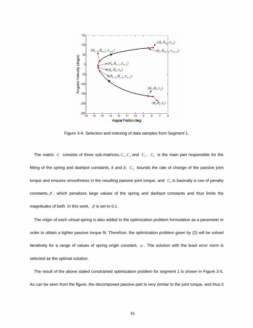
41

Figure 3-4. Selection and indexing of data samples from Segment 1.

The matrix C consists of three sub-matrices, 21 ,CC and 3C . 1C is the main part responsible for the

fitting of the spring and dashpot constants, k and b. 2C bounds the rate of change of the passive joint

torque and ensures smoothness in the resulting passive joint torque, and 3C is basically a row of penalty

constants, β , which penalizes large values of the spring and dashpot constants and thus limits the

magnitudes of both. In this work, β is set to 0.1.

The origin of each virtual spring is also added to the optimization problem formulation as a parameter in

order to obtain a tighter passive torque fit. Therefore, the optimization problem given by (2) will be solved

iteratively for a range of values of spring origin constant, α . The solution with the least error norm is

selected as the optimal solution.

The result of the above stated constrained optimization problem for segment 1 is shown in Figure 3-5.

As can be seen from the figure, the decomposed passive part is very similar to the joint torque, and thus it

42

can be stated that the behavior of the joint is mainly passive. The result of the decomposition for the

segment iS is stored in iR of the form given in (4).

[ ]6221 nxactSSpasi FFR ττθθ &= (4)

xCpas 1=τ (5)

7. Joint Torque Reference Generation

The procedure presented in the previous section decomposes the joint torques into active and passive

parts. The joint torque references for the control of the prosthesis are generated by combining this active

and passive torques. There are two major challenges to be solved. Firstly, the correct motion segment

must be selected. Secondly, after the motion segment is selected at each sampling instant a new joint

torque reference should be generated using the discrete mappings for the active and passive torque parts.

A switching system modeling approach incorporating both discrete and continuous states is used for the

reconstruction of the torque reference signal. The state chart shown in Figure 3-6 will govern the discrete

dynamics of the controller. Since the sequence of the segments is ordered (i.e., the direction of the motion

for a specific gait mode does not change), each segment can transition only to the next one, where the

transition guard function can be written as a inequality in terms of θ and θ& . The transitions between

segments take no time and the dynamics of the controller are governed by the { })(;),( Siaip Fff θθ & pair at

each sampling instant. The joint reference torque is

)(),( Sapparef Fffii

+=+= θθτττ & (6)

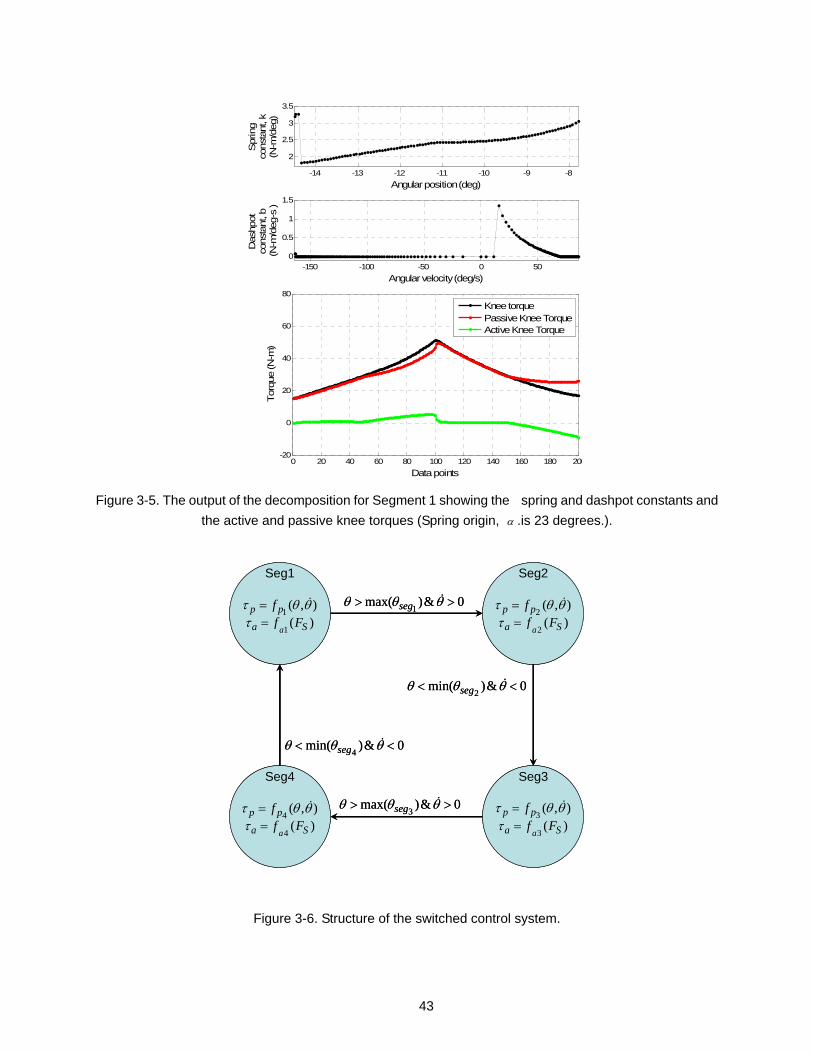
43

-14 -13 -12 -11 -10 -9 -8

2

2.5

3

3.5

Spr

ing

con

stan

t, k

(N-m

/deg

)

Angular position (deg)

-150 -100 -50 0 500

0.5

1

1.5

Das

hpot

co

nsta

nt, b

(N

-m/d

eg-s

)Angular velocity (deg/s)

0 20 40 60 80 100 120 140 160 180 200-20

0

20

40

60

80

Torq

ue (N

-m)

Data points

Knee torquePassive Knee TorqueActive Knee Torque

Figure 3-5. The output of the decomposition for Segment 1 showing the spring and dashpot constants and

the active and passive knee torques (Spring origin, α .is 23 degrees.).

Seg1

),(1

θθτ &pp f=)(

1 Sa Ffa

=τ

Seg2

),(2

θθτ &pp f=)(

2 Sa Ffa

=τ

Seg3

),(3

θθτ &pp f=)(

3 Sa Ffa

=τ

Seg4

),(4

θθτ &pp f=)(

4 Sa Ffa

=τ

0&)max(1

>> θθθ &seg

0&)max(3

>> θθθ &seg

0&)min(4

<< θθθ &seg

0&)min(2

<< θθθ &seg

Seg1

),(1

θθτ &pp f=)(

1 Sa Ffa

=τ

Seg2

),(2

θθτ &pp f=)(

2 Sa Ffa

=τ

Seg3

),(3

θθτ &pp f=)(

3 Sa Ffa

=τ

Seg4

),(4

θθτ &pp f=)(

4 Sa Ffa

=τ

0&)max(1

>> θθθ &seg

0&)max(3

>> θθθ &seg

0&)min(4

<< θθθ &seg

0&)min(2

<< θθθ &seg

Figure 3-6. Structure of the switched control system.

44

The decomposition algorithm presented in this work gives the result matrix, R, for each segment. The

discrete data in R is used to construct the joint torque reference for the continuous measurements of

another trial in the same gait mode. At each sampling instant of the algorithm, the measurement vector

TmSmSmm FFm ],,,[ _2_1θθ &= will be acquired. For the reconstruction of the passive knee torque part, the

Euclidian error norm between the Tmm ][ θθ & and the angular position and velocities of all the samples in

that segment Tii ][ θθ & is calculated as shown in (7) and stored in the vector e .

22 )()( imimie θθθθ && −+−= (7)

Then two elements of this vector with the least error norm are found and the passive knee torque

reference is found as a weighted linear combination of the passive knee torques corresponding to these

points. The reconstruction of the active knee torque part is similar where only },,{ pasτθθ & is changed with

},,{ 21 actSS FF τ .

8. Implementation and Experimental Validation

In order to generate appropriate kinematic and kinetic data for the design of the controller and for testing

of the approach, gait experiments were conducted in the Biomechanics and Sports Medicine Laboratory of

the University of Tennessee at Knoxville. The experimental setup consisted of a 7-camera 240 Hz VICON

MX system and 2 AMTI multiaxis force platforms. As is standard in such a setup, hip, knee and ankle

angles were measured via the cameras, the ground reaction force was measured using the multiaxis force

plates, and the joint torques and forces were computed in post-processing via inverse dynamics, based on

inertial parameters estimated with lookup tables. The sampling rate for the cameras and the force plates

were 100 Hz and 1000 Hz, respectively. Data collection consisted of four trials each slow walking (WS),

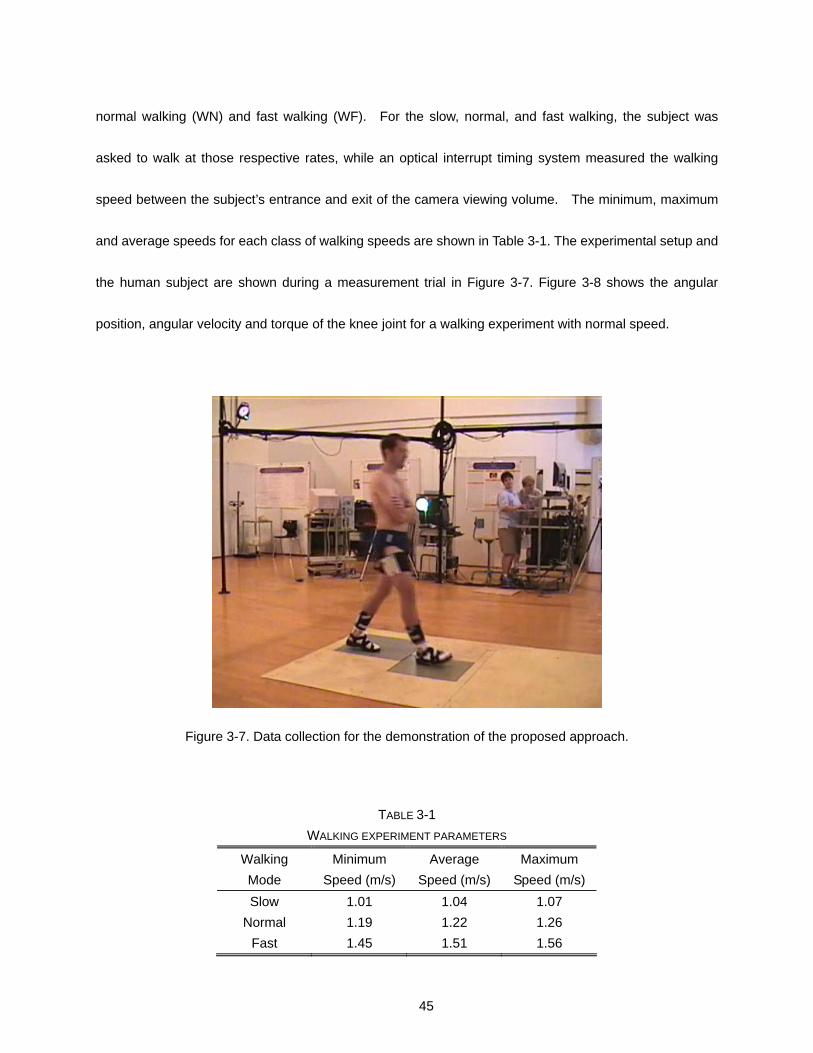
45

normal walking (WN) and fast walking (WF). For the slow, normal, and fast walking, the subject was

asked to walk at those respective rates, while an optical interrupt timing system measured the walking

speed between the subject’s entrance and exit of the camera viewing volume. The minimum, maximum

and average speeds for each class of walking speeds are shown in Table 3-1. The experimental setup and

the human subject are shown during a measurement trial in Figure 3-7. Figure 3-8 shows the angular

position, angular velocity and torque of the knee joint for a walking experiment with normal speed.

Figure 3-7. Data collection for the demonstration of the proposed approach.

TABLE 3-1 WALKING EXPERIMENT PARAMETERS

Walking Mode

Minimum Speed (m/s)

Average Speed (m/s)

Maximum Speed (m/s)

Slow 1.01 1.04 1.07 Normal 1.19 1.22 1.26

Fast 1.45 1.51 1.56

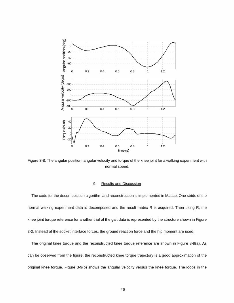
46

0 0.2 0.4 0.6 0.8 1 1.2

-60

-40

-20

0

Ang

ular

pos

ition

(deg

)

0 0.2 0.4 0.6 0.8 1 1.2-400

-200

0

200

400

Ang

ular

vel

ocity

(deg

/s)

0 0.2 0.4 0.6 0.8 1 1.2

-20

0

20

40

Torq

ue (N

-m)

time (s)

Figure 3-8. The angular position, angular velocity and torque of the knee joint for a walking experiment with normal speed.

9. Results and Discussion

The code for the decomposition algorithm and reconstruction is implemented in Matlab. One stride of the

normal walking experiment data is decomposed and the result matrix R is acquired. Then using R, the

knee joint torque reference for another trial of the gait data is represented by the structure shown in Figure

3-2. Instead of the socket interface forces, the ground reaction force and the hip moment are used.

The original knee torque and the reconstructed knee torque reference are shown in Figure 3-9(a). As

can be observed from the figure, the reconstructed knee torque trajectory is a good approximation of the

original knee torque. Figure 3-9(b) shows the angular velocity versus the knee torque. The loops in the

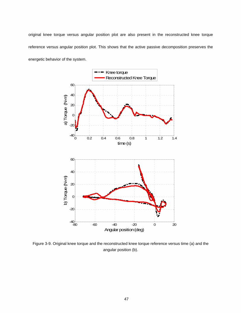
47

original knee torque versus angular position plot are also present in the reconstructed knee torque

reference versus angular position plot. This shows that the active passive decomposition preserves the

energetic behavior of the system.

0 0.2 0.4 0.6 0.8 1 1.2 1.4-40

-20

0

20

40

60

a) T

orqu

e (N

-m)

time (s)

-80 -60 -40 -20 0 20-40

-20

0

20

40

60

Angular position (deg)

b) T

orqu

e (N

-m)

Knee torqueReconstructed Knee Torque

Figure 3-9. Original knee torque and the reconstructed knee torque reference versus time (a) and the angular position (b).

48

10. Conclusion

This paper proposes a method for the control of a powered transfemoral prosthesis. The approach is

based on the decomposition of knee torque into 1) a fundamentally passive component, which is an

algebraic function of joint angle and angular velocity, and 2) an active component, which is an algebraic

function of the measured forces between the user socket and the prosthesis. The paper presents a

method for decomposing measured data into these passive and active algebraic functions, and describes

a method for generating real-time torque trajectories based on these functions and the measured joint

angles and angular velocities and interaction forces. The effectiveness of the approach is demonstrated

on measured biomechanical data. Future work will utilize the proposed approach for the real-time control

of the powered transfemoral prosthesis.

11. References

Aeyels, B., Van Petegem, W., Sloten, V., Van der Perre, G. and Peeraer, L., EMG-based finite state approach for a microcomputer-controlled above-knee prosthesis, Annual International Conference of the IEEE Engineering in Medicine and Biology, Proceedings of IEEE Engineering in Medicine and Biology, 1995.

DeVita, P., Torry M., Glover, K.L., and Speroni, D.L. A Functional Knee Brace Alters Joint Torque and Power Patterns during Walking and Running, Journal of Biomechanics, vol. 29, no. 5, pp. 583-588, 1996.

Donath, M., Proportional EMG Control for Above-Knee Prosthesis’, Department of Mechanical Engineering Masters Thesis, MIT, 1974.

Fite, K.B., Mitchell, J., Barth, E.J., and Goldfarb, M. A Unified Force Controller for a Proportional-Injector Direct-Injection Monopropellant-Powered Actuator, ASME Journal of Dynamic Systems, Measurement and Control, vol. 128, no. 1, pp. 159-164, 2006.

Fite, K.B., and Goldfarb, M. Design and Energetic Characterization of a Proportional-Injector Monopropellant-Powered Actuator, IEEE/ASME Transactions on Mechatronics, vol. 11, no. 2, pp. 196-204, 2006.

49

Flowers, W.C., A Man-Interactive Simulator System for Above-Knee Prosthetics Studies, Department of Mechanical Engineering PhD Thesis, MIT, 1973.

Flowers, W.C., and Mann, R.W. Electrohydraulic knee-torque controller for a prosthesis simulator. ASME Journal of Biomechanical Engineering, vol. 99, no. 4, pp. 3-8, 1977.

Goldfarb, M., Barth, E.J., Gogola, M.A., and Wehrmeyer, J.A.. Design and Energetic Characterization of a Liquid-Propellant-Powered Actuator for Self-Powered Robots, IEEE/ASME Transactions on Mechatronics, vol. 8, no. 2, pp. 254-262, 2003.

Grimes, D. L. An Active Multi-Mode Above Knee Prosthesis Controller. Department of Mechanical Engineering PhD Thesis, MIT, 1979.

Grimes, D. L., Flowers, W. C., and Donath, M. Feasibility of an active control scheme for above knee prostheses. ASME Journal of Biomechanical Engineering, vol. 99, no. 4, pp. 215-221, 1977.

Jacobs, R., Bobbert, M.F., van Ingen Schenau, G.J. Mechanical output from individual muscles during explosive leg extensions: the role of biarticular muscles. Journal of Biomechanics, vol. 29, no. 4, pp. 513-523, 1996.

Myers, D. and Moskowitz, G., Myoelectric pattern recognition for use in the volitional control of above-knee prosthesis, IEEE Trans. Syst. Man Cybern., Vol. SMC-11 No. 4, pp. 296-302, 1981.

Myers, D. and Moskowitz, G., Active EMG-controlled A/K prosthesis. Control aspects of prosthetics and orthotics, Proceedings of the IFAC Symposium, Columbus, OH, 1983.

Nadeau, S., McFadyen, B.J., and Malouin, F. Frontal and sagittal plane analyses of the stair climbing task in healthy adults aged over 40 years: What are the challenges compared to level walking? Clinical Biomechanics, vol. 18, no. 10, pp. 950-959, 2003.

Nagano, A., Ishige, Y., and Fukashiro, S. Comparison of new approaches to estimate mechanical output of individual joints in vertical jumps. Journal of Biomechanics, vol. 31, no. 10, pp. 951-955, 1998.

Prilutsky, B.I., Petrova, L.N., and Raitsin, L.M. Comparison of mechanical energy expenditure of joint moments and muscle forces during human locomotion. Journal of Biomechanics, vol. 29, no. 4, pp. 405-415, 1996.

Popovic, D. and Schwirtlich, L. Belgrade active A/K prosthesis, in de Vries, J. (Ed.), Electrophysiological Kinesiology, Intern. Congress Ser. No. 804, Excerpta Medica, Amsterdam, The Netherlands, pp. 337–343, 1988.

Riener, R., Rabuffetti, M., and Frigo, C. Joint powers in stair climbing at different slopes. Proceedings of the IEEE International Conference on Engineering in Medicine and Biology, vol. 1, p. 530, 1999.

50

Shields, B.L., Fite, K., and Goldfarb, M. Design, Control, and Energetic Characterization of a Solenoid Injected Monopropellant Powered Actuator, IEEE/ASME Transactions on Mechatronics, vol. 11, no. 4, pp. 477-487, 2006.

Stein, J.L. Design Issues in the Stance Phase Control of Above-Knee Prostheses. Department of Mechanical Engineering PhD Thesis, MIT, 1983

Stein, J.L., and Flowers, W.C. Stance phase control of above-knee prostheses: knee control versus SACH foot design. Journal of Biomechanics, vol. 20, no. 1, pp. 19-28, 1987.

Slotine, J.J.E., and Li, W., Applied Nonlinear Control, Prentice-Hall, 1991.

Sup, F., and Goldfarb, M. Design of a Pneumatically Actuated Transfemoral Prosthesis. Proceedings of ASME International Mechanical Engineering Conference and Exposition, IMECE2006-15707, 2006.

Triolo, R. and Moskowitz, G., Autoregressive EMG analysis and prosthetic control, Proceedings of the 35th Annual Conference on Engineering in Medicine and Biology, Philadelphia, PA, 1982.

Winter, D.A. The biomechanics and motor control of human gait: normal, elderly and pathological, University of Waterloo Press, 2nd ed, 1991.

Winter, D. A. and Sienko, S. E. Biomechanics of below-knee amputee gait. J. Biomechanics. 21, 361–367, 1988.

51

CHAPTER IV

THREE AXIS SOCKET LOAD CELL CALIBRATION

The proposed control algorithm for the powered prosthesis determines the user intent based on the

characteristic shape of the force and moment vector of interaction between the user and prosthesis.

Moreover, the active passive decomposition based control for generating the joint torques uses the force

and moment vector in order to map the active part of the joint torques. Therefore, the precise

measurement of the force and moment vector is a very critical task for the control performance of the

whole powered prosthesis. This force and moment vector is measured by a three axis socket load cell,

which is stationed just above the knee. It measures the sagittal plane moment, SM , frontal plane moment,

FM , and the vertical axial load, F , above the knee. Due to the interaction of different forces and

moments, calibration is necessary in order to make precise measurements. For the calibration of the

socket load cell, an experimental setup consisting of two orthogonal bars is constructed. The socket load

cell is at the intersection of the two bars. One of the bars is connected to two pneumatic pistons which can

exert different forces and moments on a plane to the load cell. The other bar can exert different moments

and forces to the load cell by changing the weights on the bar (See Figure 4-1).

576 measurements ranging from -400N to 1100N for the axial load, -50Nm to 50Nm for the frontal

plane moment and -120Nm to 120Nm for the sagittal plane moment is done. The analog outputs for the

three measurement channels are recorded using Matlab/Simulink and data acqusition board. First order

linear least square fits were fit to the raw data using the standard definition for least squares:

52

( ) YT ⋅Φ⋅Φ=−1

θ (1)

where,

⎟⎟⎟⎟⎟

⎠

⎞

⎜⎜⎜⎜⎜

⎝

⎛

=Φ

S

F

MF

MF 0

(2)

and

( )SF MMFY = (3)

Using the calibration data in the linear least squares equation the following matrix results:

⎟⎟⎟⎟⎟

⎠

⎞

⎜⎜⎜⎜⎜

⎝

⎛

−−

−−−

−−−

−

=

1.214.07.32.05.06.839.04.231.166.301.54.163

θ (4)

The results for the axial load, frontal plane moment and sagittal plane moment are shown in Figure 4-2

to Figure 4-4, respectively. It is seen that the square root of the mean squared error is 81.6 N for the axial

load measurement, 3.9 Nm for the sagittal plane moment measurement and 1.9 Nm for the frontal plane

moment measurement. It is also observed that higher order fits to the raw data does not increase the fitting

accuracy substantially and it is decided to use the first order linear fitting.

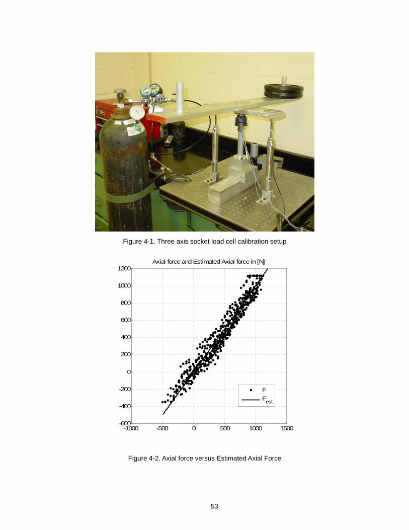
53

Figure 4-1. Three axis socket load cell calibration setup

-1000 -500 0 500 1000 1500-600

-400

-200

0

200

400

600

800

1000

1200Axial force and Estimated Axial force in [N]

FFest

Figure 4-2. Axial force versus Estimated Axial Force

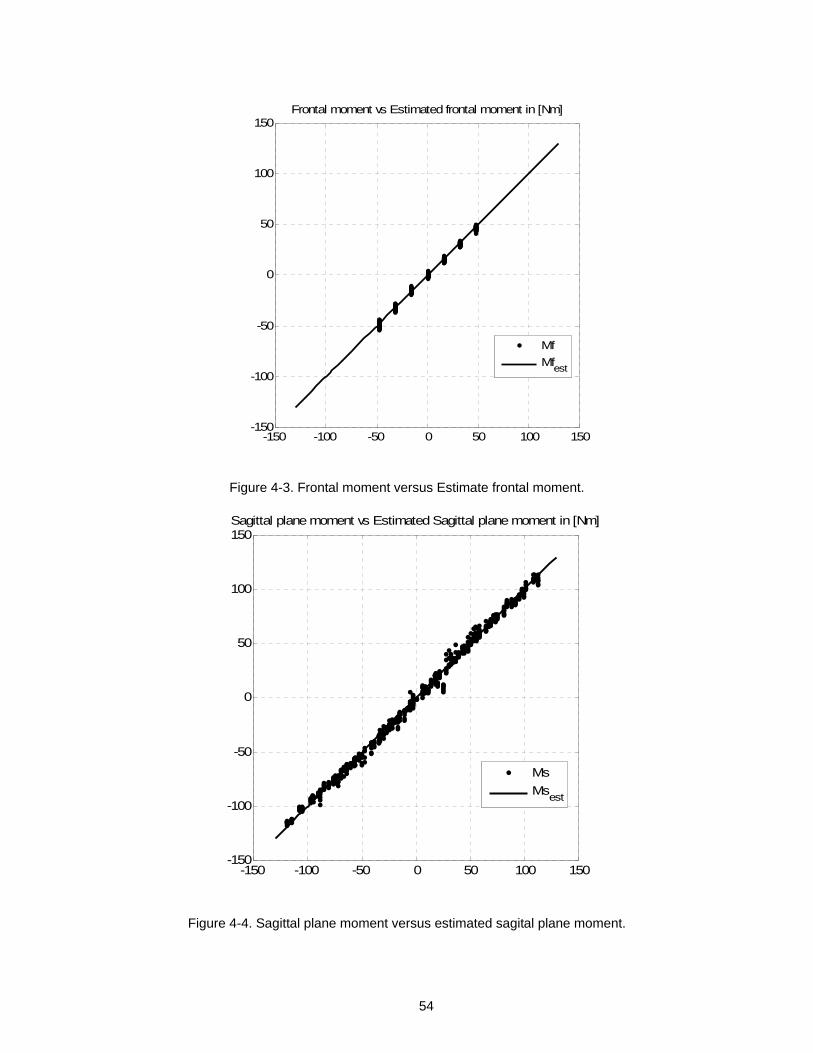
54

-150 -100 -50 0 50 100 150-150

-100

-50

0

50

100

150Frontal moment vs Estimated frontal moment in [Nm]

MfMfest

Figure 4-3. Frontal moment versus Estimate frontal moment.

-150 -100 -50 0 50 100 150-150

-100

-50

0

50

100

150Sagittal plane moment vs Estimated Sagittal plane moment in [Nm]

MsMsest

Figure 4-4. Sagittal plane moment versus estimated sagital plane moment.

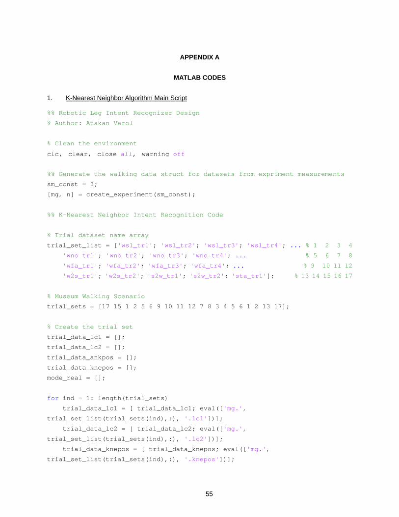
55

APPENDIX A

MATLAB CODES

1. K-Nearest Neighbor Algorithm Main Script

%% Robotic Leg Intent Recognizer Design

% Author: Atakan Varol % Clean the environment clc, clear, close all, warning off %% Generate the walking data struct for datasets from expriment measurements sm_const = 3; [mg, n] = create_experiment(sm_const); %% K-Nearest Neighbor Intent Recognition Code % Trial dataset name array trial_set_list = ['wsl_tr1'; 'wsl_tr2'; 'wsl_tr3'; 'wsl_tr4'; ... % 1 2 3 4 'wno_tr1'; 'wno_tr2'; 'wno_tr3'; 'wno_tr4'; ... % 5 6 7 8 'wfa_tr1'; 'wfa_tr2'; 'wfa_tr3'; 'wfa_tr4'; ... % 9 10 11 12 'w2s_tr1'; 'w2s_tr2'; 's2w_tr1'; 's2w_tr2'; 'sta_tr1']; % 13 14 15 16 17 % Museum Walking Scenario trial_sets = [17 15 1 2 5 6 9 10 11 12 7 8 3 4 5 6 1 2 13 17];

% Create the trial set trial_data_lc1 = []; trial_data_lc2 = []; trial_data_ankpos = []; trial_data_knepos = []; mode_real = []; for ind = 1: length(trial_sets) trial_data_lc1 = [ trial_data_lc1; eval(['mg.',

trial_set_list(trial_sets(ind),:), '.lc1'])]; trial_data_lc2 = [ trial_data_lc2; eval(['mg.',

trial_set_list(trial_sets(ind),:), '.lc2'])]; trial_data_knepos = [ trial_data_knepos; eval(['mg.',

trial_set_list(trial_sets(ind),:), '.knepos'])];

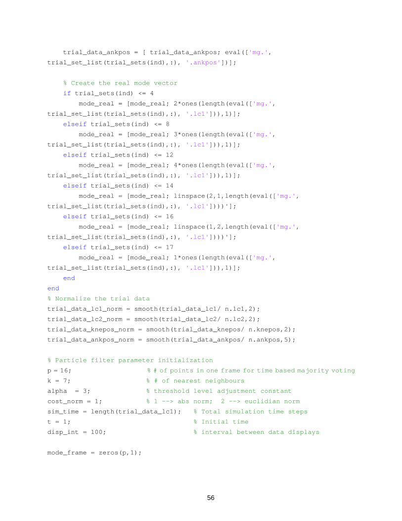
56

trial_data_ankpos = [ trial_data_ankpos; eval(['mg.',

trial_set_list(trial_sets(ind),:), '.ankpos'])]; % Create the real mode vector if trial_sets(ind) <= 4 mode_real = [mode_real; 2*ones(length(eval(['mg.',

trial_set_list(trial_sets(ind),:), '.lc1'])),1)]; elseif trial_sets(ind) <= 8 mode_real = [mode_real; 3*ones(length(eval(['mg.',

trial_set_list(trial_sets(ind),:), '.lc1'])),1)]; elseif trial_sets(ind) <= 12 mode_real = [mode_real; 4*ones(length(eval(['mg.',

trial_set_list(trial_sets(ind),:), '.lc1'])),1)]; elseif trial_sets(ind) <= 14 mode_real = [mode_real; linspace(2,1,length(eval(['mg.',

trial_set_list(trial_sets(ind),:), '.lc1'])))']; elseif trial_sets(ind) <= 16 mode_real = [mode_real; linspace(1,2,length(eval(['mg.',

trial_set_list(trial_sets(ind),:), '.lc1'])))']; elseif trial_sets(ind) <= 17 mode_real = [mode_real; 1*ones(length(eval(['mg.',

trial_set_list(trial_sets(ind),:), '.lc1'])),1)]; end end % Normalize the trial data trial_data_lc1_norm = smooth(trial_data_lc1/ n.lc1,2); trial_data_lc2_norm = smooth(trial_data_lc2/ n.lc2,2); trial_data_knepos_norm = smooth(trial_data_knepos/ n.knepos,2); trial_data_ankpos_norm = smooth(trial_data_ankpos/ n.ankpos,5); % Particle filter parameter initialization p = 16; % # of points in one frame for time based majority voting k = 7; % # of nearest neighbours alpha = 3; % threshold level adjustment constant cost_norm = 1; % 1 --> abs norm; 2 --> euclidian norm sim_time = length(trial_data_lc1); % Total simulation time steps t = 1; % Initial time disp_int = 100; % interval between data displays mode_frame = zeros(p,1);

57

%Prepare the data matrix mg.dataset_list = ['ws1'; 'ws2';'ws3'; 'wn1'; 'wn2';'wn4'; 'wf1'; 'wf2'; 'wf3';

'st1']; dataset_len = []; dataset_lc1_arr = []; dataset_lc2_arr = []; dataset_knepos_arr = []; dataset_ankpos_arr = []; for t = 1 : length(mg.dataset_list) dataset_len = [dataset_len, eval(['mg.' , mg.dataset_list(t,:),'.len'])]; dataset_lc1_arr = [dataset_lc1_arr; eval(['mg.' ,

mg.dataset_list(t,:),'.lc1_norm'])]; dataset_lc2_arr = [dataset_lc2_arr; eval(['mg.' ,

mg.dataset_list(t,:),'.lc2_norm'])]; dataset_knepos_arr = [dataset_knepos_arr; eval(['mg.' ,

mg.dataset_list(t,:),'.knepos_norm'])]; dataset_ankpos_arr = [dataset_ankpos_arr; eval(['mg.' ,

mg.dataset_list(t,:),'.ankpos_norm'])]; end % KNN Algorithm main loop for t = 1:sim_time % Cost calculation if cost_norm == 1 % abs norm cost = abs(trial_data_lc1_norm(t) - dataset_lc1_arr) + ... abs(trial_data_lc2_norm(t) - dataset_lc2_arr) + ... abs(trial_data_knepos_norm(t) - dataset_knepos_arr) + ... abs(trial_data_ankpos_norm(t) - dataset_ankpos_arr); elseif cost_norm == 2 % euclidian norm cost = sqrt( (trial_data_lc1_norm(t) -dataset_lc1_arr).^2 + ... (trial_data_lc2_norm(t) - dataset_lc2_arr).^2 + ... (trial_data_knepos_norm(t) - dataset_knepos_arr).^2 + ... (trial_data_ankpos_norm(t) - dataset_ankpos_arr).^2); end % Mode estimation for the iteration [cost_val, cost_ind] = sort(cost); mode = zeros(4,1); % 1 --> standing ; 2 --> slow; 3 --> medium; 4 --> fast for ind = 1:k if cost_ind(ind) <= sum(dataset_len(1:3)) mode(2) = mode(2) + 1; elseif cost_ind(ind) <= sum(dataset_len(1:6))

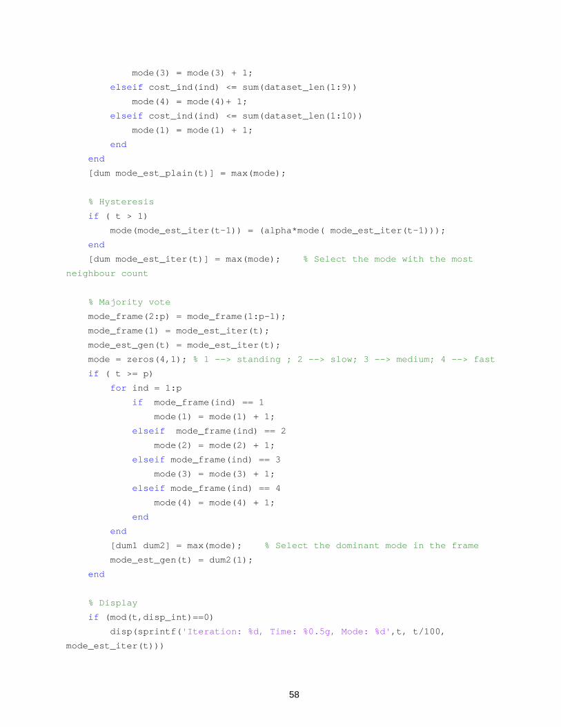
58

mode(3) = mode(3) + 1; elseif cost_ind(ind) <= sum(dataset_len(1:9)) mode(4) = mode(4)+ 1; elseif cost_ind(ind) <= sum(dataset_len(1:10)) mode(1) = mode(1) + 1; end end [dum mode_est_plain(t)] = max(mode); % Hysteresis if ( t > 1) mode(mode_est_iter(t-1)) = (alpha*mode( mode_est_iter(t-1))); end [dum mode_est_iter(t)] = max(mode); % Select the mode with the most

neighbour count % Majority vote mode_frame(2:p) = mode_frame(1:p-1); mode_frame(1) = mode_est_iter(t); mode_est_gen(t) = mode_est_iter(t); mode = zeros(4,1); % 1 --> standing ; 2 --> slow; 3 --> medium; 4 --> fast if ( t >= p) for ind = 1:p if mode_frame(ind) == 1 mode(1) = mode(1) + 1; elseif mode_frame(ind) == 2 mode(2) = mode(2) + 1; elseif mode_frame(ind) == 3 mode(3) = mode(3) + 1; elseif mode_frame(ind) == 4 mode(4) = mode(4) + 1; end end [dum1 dum2] = max(mode); % Select the dominant mode in the frame mode_est_gen(t) = dum2(1); end % Display if (mod(t,disp_int)==0) disp(sprintf('Iteration: %d, Time: %0.5g, Mode: %d',t, t/100,

mode_est_iter(t)))

59

end end % Visualization figure(1); subplot 311, plot((1:sim_time)/100, mode_real, 'k-',(1:sim_time)/100,

mode_est_plain,'ko') title('a) Plain K-NN') ylabel('Gait mode') axis([0 30.42 0.8 4.2]) subplot 312, plot((1:sim_time)/100, mode_real, 'k-',(1:sim_time)/100,

mode_est_iter,'ko') title('b) K-NN with biasing constant') ylabel('Gait mode') axis([0 30.42 0.8 4.2]) subplot 313, plot((1:sim_time)/100, mode_real, 'k-',(1:sim_time)/100,

mode_est_gen,'ko') title('c) K-NN with biasing constant and the time based majority voting') ylabel('Gait mode') xlabel('time in s') axis([0 30.42 0.8 4.2]) legend('real mode', 'predicted mode')

60

2. Active-Passive Decomposition Procedure Main Script

%% Robotic Leg Control Design Author: Atakan Varol

% Clean the environment clc, clear, close all, warning off %% Generate the walking data struct for datasets from expriment measurements sm_const = 3; [mg, n] = create_experiment(sm_const); %% Active-passive decomposition method 1 len_data_smooth = 100; % moving average smoothing filter frame size for knepos,

knevel and knemom epsi = 1e-3; % very small number out_const = 10; % outlier const % Get the knepos, knevel and knemom - interpolate them to 10000 points knepos_int = smooth(interp([mg.wn2.knepos(end-10+1:end) ; mg.wn2.knepos;

mg.wn2.knepos(1:10)] ,100),len_data_smooth); knevel_int = smooth(interp([mg.wn2.knevel(end-10+1:end) ; mg.wn2.knevel;

mg.wn2.knevel(1:10)] ,100),len_data_smooth); knemom_int = smooth( interp([mg.wn2.knemom(end-10+1:end) ; mg.wn2.knemom;

mg.wn2.knemom(1:10)] ,100), len_data_smooth); hipmom_int = smooth( interp([mg.wn2.lc2(end-10+1:end) ; mg.wn2.lc2;

mg.wn2.lc2(1:10)] ,100), 3*len_data_smooth); gref_int= smooth( interp([mg.wn2.lc1(end-10+1:end) ; mg.wn2.lc1;

mg.wn2.lc1(1:10)] ,100), 3*len_data_smooth); knevel_int = knevel_int(1001:end-1000); knepos_int = knepos_int(1001:end-1000); knemom_int = knemom_int(1001:end-1000); hipmom_int = hipmom_int(1001:end-1000); gref_int= gref_int(1001:end-1000); % Create first linear programming problem (for the first segment) % Segment 1 with -15 degree angular position offset

61

res_norm_hist = []; for offset_seg1 = -23 ind_seg1 = 1050:3390; knepos_seg1 = knepos_int(ind_seg1); % Impose boundary value knepos_seg1_offset = knepos_seg1 - offset_seg1; % For easier

optimization formulation knevel_seg1 = knevel_int(ind_seg1); knemom_seg1 = knemom_int(ind_seg1); max_knepos_seg1 = max(knepos_seg1_offset); min_knepos_seg1 = min(knepos_seg1_offset); tr_len = 100; knepos_seg1_trial = linspace( max_knepos_seg1, min_knepos_seg1, tr_len); delta = abs(knepos_seg1_trial(2) - knepos_seg1_trial(1)); knemom_lp_seg1 = zeros(2*tr_len+1,1); mat_lp_seg1 = zeros(2*tr_len+1,3*tr_len); posind_hist = zeros(tr_len,1); velind_hist = zeros(2*tr_len,1); for t = 1:tr_len [ind1_list] = knepos_seg1_offset > knepos_seg1_trial(t) - delta/2 & ... knepos_seg1_offset < knepos_seg1_trial(t) + delta/2 & ... knevel_seg1 > 0 ; ind1 = find(ind1_list == 1, 1, 'first'); posind_hist(t) = ind1; velind_hist(t) = ind1; [ind2_list] = knepos_seg1_offset > knepos_seg1_trial(t) - delta/2 & ... knepos_seg1_offset < knepos_seg1_trial(t) + delta/2 & ... knevel_seg1 < 0; ind2 = find(ind2_list == 1, 1, 'last'); velind_hist(2*tr_len + 1 - t) = ind2; end posind_hist = posind_hist(end:-1:1); velind_hist = velind_hist(end:-1:1); knemom_lp_seg1 = [ knemom_seg1(velind_hist); ... knemom_seg1(velind_hist(1:end-1)) - knemom_seg1(velind_hist(2:end)) ;

0]; mat_lp_seg1 = [ [ diag(knepos_seg1_offset(posind_hist));

diag(knepos_seg1_offset(posind_hist(end:-1:1))) ], ...

62

diag(knevel_seg1(velind_hist))]; mat_lp_seg1 = [mat_lp_seg1 ; [ mat_lp_seg1(1:end-1,:) -

mat_lp_seg1(2:end,:)]]; mat_lp_seg1 = [mat_lp_seg1 ; 0.2*ones(1,300)]; options = optimset('MaxIter', 2e3); [kb_list_seg1 res_norm res eflag] = lsqlin(mat_lp_seg1, knemom_lp_seg1, [],

[],[],[],zeros(300,1),100*ones(300,1),[],options) ; kb_list_seg1(kb_list_seg1 < epsi) = 0; k_seg1 = kb_list_seg1(1:100); b_seg1 = kb_list_seg1(101:300); knemom_fit_seg1 = mat_lp_seg1(1:end-2*tr_len,:)*kb_list_seg1(1:end); res_norm_hist = [res_norm_hist res_norm]; end [val, ind ] = min(res_norm_hist) indlist_gen = []; indlist_gen = [indlist_gen ; (1049 + velind_hist)]; indlist_seg1 = 1049+velind_hist; figure(1), subplot 311, plot(knepos_seg1(posind_hist), k_seg1, 'r.-'), ylabel('Spring constant, k'), xlabel('Angular position (deg)'), axis tight, grid on subplot 312, plot(knevel_seg1(velind_hist), b_seg1, 'r.-'), ylabel('Dashpot constant, k'), xlabel('Angular position (deg)'), axis tight, grid on subplot 313, plot(1:length(knemom_lp_seg1)-2*tr_len,

knemom_lp_seg1(1:end-2*tr_len) , 'r.',... 1:length(knemom_lp_seg1)-2*tr_len, knemom_fit_seg1, 'g.','LineWidth',2),

grid on % Create the second linear programming problem (for the second segment) % Segment 2 with -15 degree angular position offset res_norm_hist = []; for offset_seg2 = -23 ind_seg2 = 3391:6830; knepos_seg2 = knepos_int(ind_seg2); % Impose boundary value

knepos_seg2_offset = knepos_seg2 - offset_seg2; % For easier optimization

formulation knevel_seg2 = knevel_int(ind_seg2); knemom_seg2 = knemom_int(ind_seg2);

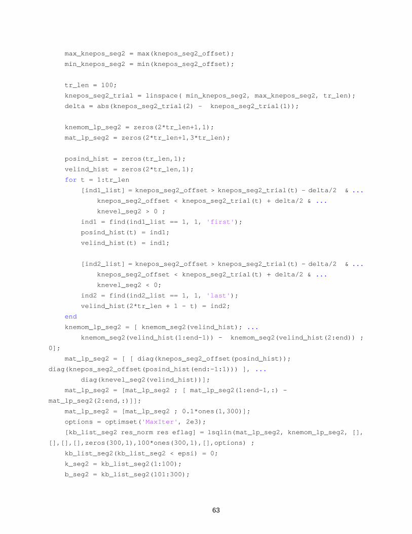
63

max_knepos_seg2 = max(knepos_seg2_offset); min_knepos_seg2 = min(knepos_seg2_offset); tr_len = 100; knepos_seg2_trial = linspace( min_knepos_seg2, max_knepos_seg2, tr_len); delta = abs(knepos_seg2_trial(2) - knepos_seg2_trial(1)); knemom_lp_seg2 = zeros(2*tr_len+1,1); mat_lp_seg2 = zeros(2*tr_len+1,3*tr_len); posind_hist = zeros(tr_len,1); velind_hist = zeros(2*tr_len,1); for t = 1:tr_len [ind1_list] = knepos_seg2_offset > knepos_seg2_trial(t) - delta/2 & ... knepos_seg2_offset < knepos_seg2_trial(t) + delta/2 & ... knevel_seg2 > 0 ; ind1 = find(ind1_list == 1, 1, 'first'); posind_hist(t) = ind1; velind_hist(t) = ind1; [ind2_list] = knepos_seg2_offset > knepos_seg2_trial(t) - delta/2 & ... knepos_seg2_offset < knepos_seg2_trial(t) + delta/2 & ... knevel_seg2 < 0; ind2 = find(ind2_list == 1, 1, 'last'); velind_hist(2*tr_len + 1 - t) = ind2; end knemom_lp_seg2 = [ knemom_seg2(velind_hist); ... knemom_seg2(velind_hist(1:end-1)) - knemom_seg2(velind_hist(2:end)) ;

0]; mat_lp_seg2 = [ [ diag(knepos_seg2_offset(posind_hist));

diag(knepos_seg2_offset(posind_hist(end:-1:1))) ], ... diag(knevel_seg2(velind_hist))]; mat_lp_seg2 = [mat_lp_seg2 ; [ mat_lp_seg2(1:end-1,:) -

mat_lp_seg2(2:end,:)]]; mat_lp_seg2 = [mat_lp_seg2 ; 0.1*ones(1,300)]; options = optimset('MaxIter', 2e3); [kb_list_seg2 res_norm res eflag] = lsqlin(mat_lp_seg2, knemom_lp_seg2, [],

[],[],[],zeros(300,1),100*ones(300,1),[],options) ; kb_list_seg2(kb_list_seg2 < epsi) = 0; k_seg2 = kb_list_seg2(1:100); b_seg2 = kb_list_seg2(101:300);

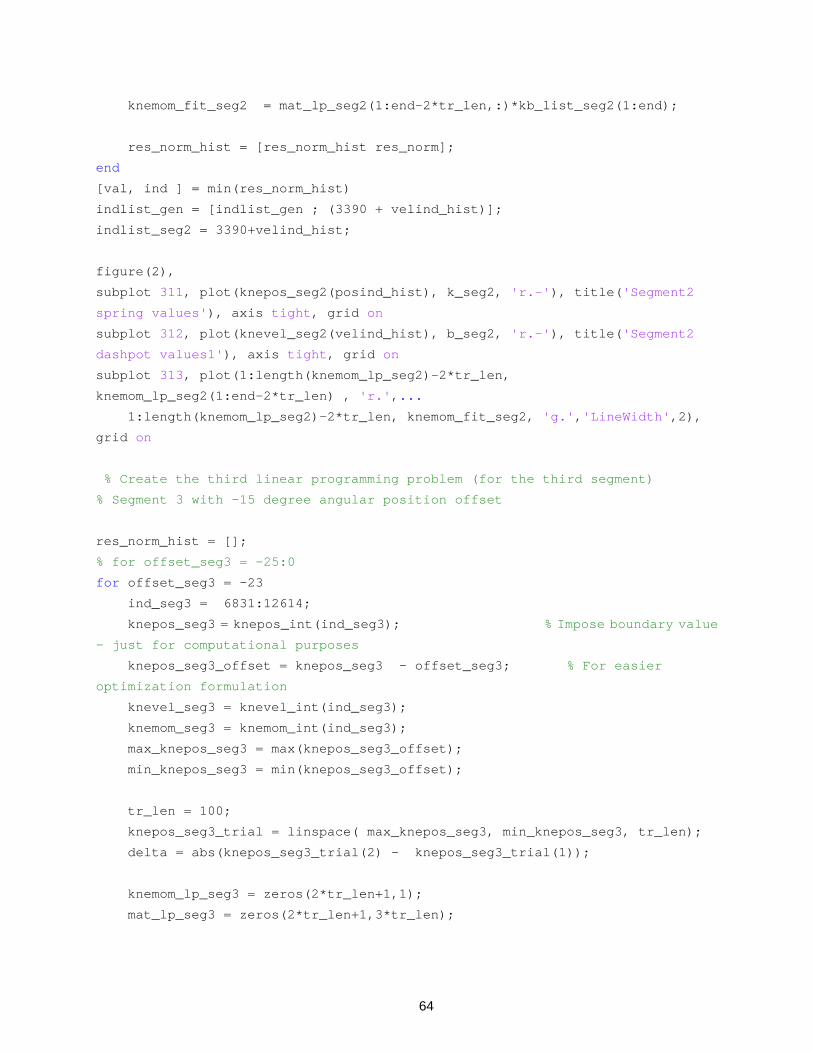
64

knemom_fit_seg2 = mat_lp_seg2(1:end-2*tr_len,:)*kb_list_seg2(1:end); res_norm_hist = [res_norm_hist res_norm]; end [val, ind ] = min(res_norm_hist) indlist_gen = [indlist_gen ; (3390 + velind_hist)]; indlist_seg2 = 3390+velind_hist; figure(2), subplot 311, plot(knepos_seg2(posind_hist), k_seg2, 'r.-'), title('Segment2

spring values'), axis tight, grid on subplot 312, plot(knevel_seg2(velind_hist), b_seg2, 'r.-'), title('Segment2

dashpot values1'), axis tight, grid on subplot 313, plot(1:length(knemom_lp_seg2)-2*tr_len,

knemom_lp_seg2(1:end-2*tr_len) , 'r.',... 1:length(knemom_lp_seg2)-2*tr_len, knemom_fit_seg2, 'g.','LineWidth',2),

grid on % Create the third linear programming problem (for the third segment) % Segment 3 with -15 degree angular position offset res_norm_hist = []; % for offset_seg3 = -25:0 for offset_seg3 = -23 ind_seg3 = 6831:12614; knepos_seg3 = knepos_int(ind_seg3); % Impose boundary value

- just for computational purposes knepos_seg3_offset = knepos_seg3 - offset_seg3; % For easier

optimization formulation knevel_seg3 = knevel_int(ind_seg3); knemom_seg3 = knemom_int(ind_seg3); max_knepos_seg3 = max(knepos_seg3_offset); min_knepos_seg3 = min(knepos_seg3_offset); tr_len = 100; knepos_seg3_trial = linspace( max_knepos_seg3, min_knepos_seg3, tr_len); delta = abs(knepos_seg3_trial(2) - knepos_seg3_trial(1)); knemom_lp_seg3 = zeros(2*tr_len+1,1); mat_lp_seg3 = zeros(2*tr_len+1,3*tr_len);

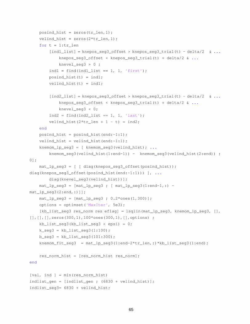
65

posind_hist = zeros(tr_len,1); velind_hist = zeros(2*tr_len,1); for t = 1:tr_len [ind1_list] = knepos_seg3_offset > knepos_seg3_trial(t) - delta/2 & ... knepos_seg3_offset < knepos_seg3_trial(t) + delta/2 & ... knevel_seg3 > 0 ; ind1 = find(ind1_list == 1, 1, 'first'); posind_hist(t) = ind1; velind_hist(t) = ind1; [ind2_list] = knepos_seg3_offset > knepos_seg3_trial(t) - delta/2 & ... knepos_seg3_offset < knepos_seg3_trial(t) + delta/2 & ... knevel_seg3 < 0; ind2 = find(ind2_list == 1, 1, 'last'); velind_hist(2*tr_len + 1 - t) = ind2; end posind_hist = posind_hist(end:-1:1); velind_hist = velind_hist(end:-1:1); knemom_lp_seg3 = [ knemom_seg3(velind_hist); ... knemom_seg3(velind_hist(1:end-1)) - knemom_seg3(velind_hist(2:end)) ;

0]; mat_lp_seg3 = [ [ diag(knepos_seg3_offset(posind_hist));

diag(knepos_seg3_offset(posind_hist(end:-1:1))) ], ... diag(knevel_seg3(velind_hist))]; mat_lp_seg3 = [mat_lp_seg3 ; [ mat_lp_seg3(1:end-1,:) -

mat_lp_seg3(2:end,:)]]; mat_lp_seg3 = [mat_lp_seg3 ; 0.2*ones(1,300)]; options = optimset('MaxIter', 5e3); [kb_list_seg3 res_norm res eflag] = lsqlin(mat_lp_seg3, knemom_lp_seg3, [],

[],[],[],zeros(300,1),100*ones(300,1),[],options) ; kb_list_seg3(kb_list_seg3 < epsi) = 0; k_seg3 = kb_list_seg3(1:100); b_seg3 = kb_list_seg3(101:300); knemom_fit_seg3 = mat_lp_seg3(1:end-2*tr_len,:)*kb_list_seg3(1:end); res_norm_hist = [res_norm_hist res_norm]; end [val, ind ] = min(res_norm_hist) indlist_gen = [indlist_gen ; (6830 + velind_hist)]; indlist_seg3= 6830 + velind_hist;

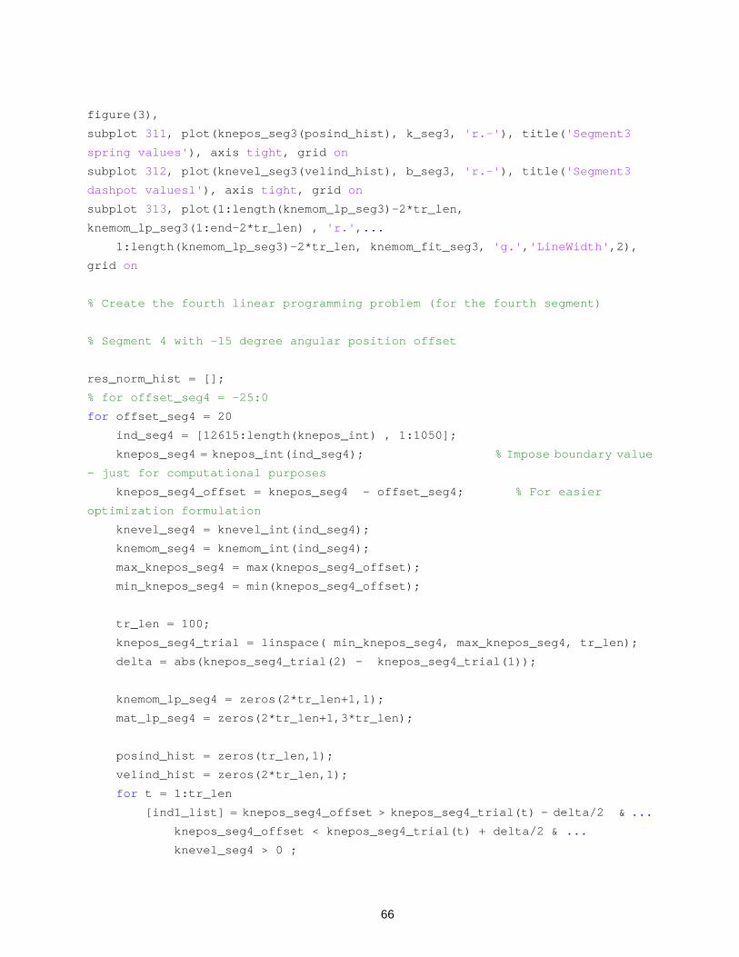
66

figure(3), subplot 311, plot(knepos_seg3(posind_hist), k_seg3, 'r.-'), title('Segment3

spring values'), axis tight, grid on subplot 312, plot(knevel_seg3(velind_hist), b_seg3, 'r.-'), title('Segment3

dashpot values1'), axis tight, grid on subplot 313, plot(1:length(knemom_lp_seg3)-2*tr_len,

knemom_lp_seg3(1:end-2*tr_len) , 'r.',... 1:length(knemom_lp_seg3)-2*tr_len, knemom_fit_seg3, 'g.','LineWidth',2),

grid on % Create the fourth linear programming problem (for the fourth segment) % Segment 4 with -15 degree angular position offset res_norm_hist = []; % for offset_seg4 = -25:0 for offset_seg4 = 20 ind_seg4 = [12615:length(knepos_int) , 1:1050]; knepos_seg4 = knepos_int(ind_seg4); % Impose boundary value

- just for computational purposes knepos_seg4_offset = knepos_seg4 - offset_seg4; % For easier

optimization formulation knevel_seg4 = knevel_int(ind_seg4); knemom_seg4 = knemom_int(ind_seg4); max_knepos_seg4 = max(knepos_seg4_offset); min_knepos_seg4 = min(knepos_seg4_offset); tr_len = 100; knepos_seg4_trial = linspace( min_knepos_seg4, max_knepos_seg4, tr_len); delta = abs(knepos_seg4_trial(2) - knepos_seg4_trial(1)); knemom_lp_seg4 = zeros(2*tr_len+1,1); mat_lp_seg4 = zeros(2*tr_len+1,3*tr_len); posind_hist = zeros(tr_len,1); velind_hist = zeros(2*tr_len,1); for t = 1:tr_len [ind1_list] = knepos_seg4_offset > knepos_seg4_trial(t) - delta/2 & ... knepos_seg4_offset < knepos_seg4_trial(t) + delta/2 & ... knevel_seg4 > 0 ;

67

ind1 = find(ind1_list == 1, 1, 'first'); posind_hist(t) = ind1; velind_hist(t) = ind1; [ind2_list] = knepos_seg4_offset > knepos_seg4_trial(t) - delta/2 & ... knepos_seg4_offset < knepos_seg4_trial(t) + delta/2 & ... knevel_seg4 < 0; ind2 = find(ind2_list == 1, 1, 'last'); velind_hist(2*tr_len + 1 - t) = ind2; end knemom_lp_seg4 = [ knemom_seg4(velind_hist); ... knemom_seg4(velind_hist(1:end-1)) - knemom_seg4(velind_hist(2:end)) ;

0]; mat_lp_seg4 = [ [ diag(knepos_seg4_offset(posind_hist));

diag(knepos_seg4_offset(posind_hist)) ], ... diag(knevel_seg4(velind_hist))]; mat_lp_seg4 = [mat_lp_seg4 ; [ mat_lp_seg4(1:end-1,:) -

mat_lp_seg4(2:end,:)]]; mat_lp_seg4 = [mat_lp_seg4 ; 0.2*ones(1,300)]; options = optimset('MaxIter', 2e3); [kb_list_seg4 res_norm res eflag] = lsqlin(mat_lp_seg4, knemom_lp_seg4, [],

[],[],[],zeros(300,1),100*ones(300,1),[],options) ; kb_list_seg4(kb_list_seg4 < epsi) = 0; k_seg4 = kb_list_seg4(1:100); b_seg4 = kb_list_seg4(101:300); knemom_fit_seg4 = mat_lp_seg4(1:end-2*tr_len,:)*kb_list_seg4(1:end); res_norm_hist = [res_norm_hist res_norm]; end [val, ind ] = min(res_norm_hist) indlist_gen = [indlist_gen ; (12615 + velind_hist)]; indlist_seg4 = mod(12615 + velind_hist, length(knemom_int)); figure(4), subplot 311, plot(knepos_seg4(posind_hist), k_seg4, 'r.-'), title('Segment4

spring values'), axis tight, grid on subplot 312, plot(knevel_seg4(velind_hist), b_seg4, 'r.-'), title('Segment4

dashpot values1'), axis tight, grid on

68

subplot 313, plot(1:length(knemom_lp_seg4)-2*tr_len,

knemom_lp_seg4(1:end-2*tr_len) , 'r.',... 1:length(knemom_lp_seg4)-2*tr_len, knemom_fit_seg4, 'g.','LineWidth',2),

grid on start = indlist_gen(indlist_gen > length(knepos_int)) -length(knepos_int) ; indlist_gen = [start; indlist_gen(1:end-length(start))]; knemom_pas_raw = [knemom_fit_seg1(1:200)' knemom_fit_seg2(1:200)'

knemom_fit_seg3(1:200)' knemom_fit_seg4(1:200)']; % Smooth sim('calc_active'); knemom_pas = smooth([knemom_pas(end-1000+1:end)' ;knemom_pas';

knemom_pas(1:1000)'] ,400); knemom_pas = knemom_pas(1001:end-1000); knemom_act = smooth(knemom_int - knemom_pas,400) % Plot the segments figure(5); cla hold on plot(knepos_seg1, knevel_seg1,'r.', 'Linewidth',2) plot(knepos_seg2, knevel_seg2,'g.', 'Linewidth',2) plot(knepos_seg3, knevel_seg3,'b.', 'Linewidth',2) plot(knepos_seg4, knevel_seg4,'m.', 'Linewidth',2) hold off; grid on; axis square legend('Segment 1', 'Segment 2' ,'Segment 3', 'Segment 4' ,'Location',

'BestOutside') xlabel('Angular position (deg)') ylabel('Angular velocity (deg/s)') % Plot the experiment data figure(6); cla subplot 311, plot(0.01*((1:length(mg.wn2.knepos))-1),mg.wn2.knepos,'k',

'Linewidth',2) ylabel('Angular position (deg)'), grid on , axis([0 1.37 1.1*min(mg.wn2.knepos)

1.1*max(mg.wn2.knepos)]) subplot 312, plot(0.01*((1:length(mg.wn2.knepos))-1),mg.wn2.knevel,'k',

'Linewidth',2) ylabel('Angular velocity (deg/s)'), grid on, axis([0 1.37 1.1*min(mg.wn2.knevel)

1.1*max(mg.wn2.knevel)])

69

subplot 313, plot(0.01*((1:length(mg.wn2.knepos))-1),mg.wn2.knemom,'k',

'Linewidth',2) ylabel('Torque (N-m)') , xlabel('time (s)'), grid on, axis([0 1.37

1.1*min(mg.wn2.knemom) 1.1*max(mg.wn2.knemom)]) % Reconstruct % Get the knepos, knevel and knemom - interpolate them to 10000 points for % another walking scenario knepos_int_tr = smooth(interp([mg.wn4.knepos(end-10+1:end) ; mg.wn4.knepos;

mg.wn4.knepos(1:10)] ,100),len_data_smooth); knevel_int_tr = smooth(interp([mg.wn4.knevel(end-10+1:end) ; mg.wn4.knevel;

mg.wn4.knevel(1:10)] ,100),len_data_smooth); knemom_int_tr = smooth( interp([mg.wn4.knemom(end-10+1:end) ; mg.wn4.knemom;

mg.wn4.knemom(1:10)] ,100), len_data_smooth); hipmom_int_tr = smooth( interp([mg.wn4.lc2(end-10+1:end) ; mg.wn4.lc2;

mg.wn4.lc2(1:10)] ,100), 3*len_data_smooth); gref_int_tr= smooth( interp([mg.wn4.lc1(end-10+1:end) ; mg.wn4.lc1;

mg.wn4.lc1(1:10)] ,100), 3*len_data_smooth); knevel_int_tr = knevel_int_tr(1001:end-1000); knepos_int_tr = knepos_int_tr(1001:end-1000); knemom_int_tr = knemom_int_tr(1001:end-1000); hipmom_int_tr = hipmom_int_tr(1001:end-1000); gref_int_tr = gref_int_tr(1001:end-1000); sim('decomp_reconstruct') % smooth knemom_ref knemom_ref = smooth(knemom_ref(:,2), 5); plot(knepos_int_tr(1:10:end), knemom_int_tr(1:10:end),'g-', ... knepos_int_tr(1:10:end), knemom_ref(1:end-1),'r-','LineWidth',2)

70

3. Three Axis Socket Load Cell Calibration Script

%% Three Axis Socket Load Cell Calibartion Script % Author: Atakan Varol close all clear clc load('exp_meas_nlc.mat'); % exp_meas2 contains the followin columns: % mom_sagittal mom_frontal force meas_val1 meas_val2 meas_val3 data(:,6) = data(:,6) - 1.5; %% Sagittal moment fit v1 = data(:,5); v2 = data(:,6); v3 = data(:,7); Ms = data(:,2); A = [ v1.^0 v1.^1 v2.^1 v3.^1]; x_Ms = pinv(A)*Ms; Ms_est = A*x_Ms; figure(1); subplot 311; plot(1:length(Ms),Ms,'r.',1:length(Ms),Ms_est,'g.') ; title('Ms') subplot 312; plot(1:length(Ms),Ms_est,'r.') ; title('Ms estimated') subplot 313; plot(1:length(Ms),Ms-Ms_est,'r.') ; title('Ms-Ms estimated') figure(2); plot(Ms, Ms_est,'r.' ,-130:130,-130:130,'g-','LineWidth', 2) ;

title('Ms vs Ms estimated'),axis square; grid on figure(3); bar(x_Ms) sqmav_Ms = sqrt(mean((Ms - Ms_est).^2)) %% Frontal moment fit v1 = data(:,5); v2 = data(:,6); v3 = data(:,7); Mf = data(:,3);

71

A = [ v1.^0 v1.^1 v2.^1 v3.^1]; x_Mf = pinv(A)*Mf; Mf_est = A*x_Mf; figure(4); subplot 311; plot(1:length(Mf),Mf,'r.',1:length(Mf),Mf_est,'g.') ; title('Mf') subplot 312; plot(1:length(Mf),Mf_est,'r.') ; title('Mf estimated') subplot 313; plot(1:length(Mf),Mf-Mf_est,'r.') ; title('Mf-Mf estimated') figure(5); plot(Mf, Mf_est,'r.' ,-130:130,-130:130,'g-','LineWidth', 2) ;

title('Mf vs Mf estimated'),axis square; grid on figure(6); bar(x_Mf) sqmav_Mf = sqrt(mean((Mf - Mf_est).^2)) %% Ground Reaction force fit v1 = data(:,5); v2 = data(:,6); v3 = data(:,7); F = data(:,4); A = [ v1.^0 v2.^1 ]; x_f = pinv(A)*F; F_est = A*x_f; figure(7); subplot 311; plot(1:length(F),F,'r.',1:length(F),F_est,'g.') ; title('F') subplot 312; plot(1:length(F),F_est,'r.') ; title('F estimated') subplot 313; plot(1:length(F),F-F_est,'r.') ; title('F-F estimated') figure(8); plot(F, F_est,'r.' ,-500:1200,-500:1200,'g-','LineWidth', 2) ;

title('F vs F estimated'),axis square; grid on figure(9); bar(x_f) sqmav_F = sqrt(mean((F - F_est).^2)) figure(10) [v1m,v2m] = meshgrid(-10 : 0.1 : 10, -10 : 0.1 : 10); res = x_f(1)*1 + x_f(2)*v1m + x_f(3)*v1m.^2 + x_f(4)*v2m + x_f(5)*v2m.^2; mesh(v1m, v2m, res)

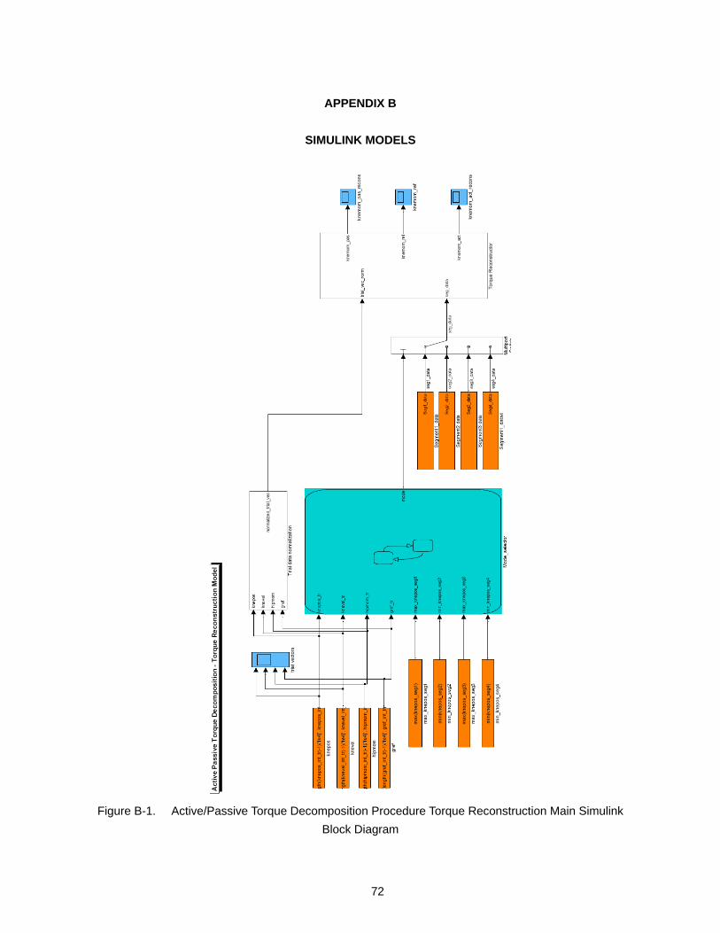
72

APPENDIX B

SIMULINK MODELS

Figure B-1. Active/Passive Torque Decomposition Procedure Torque Reconstruction Main Simulink

Block Diagram

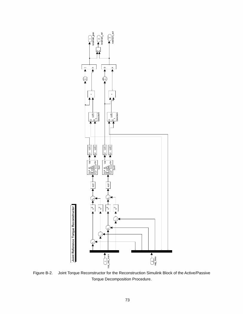
73

Figure B-2. Joint Torque Reconstructor for the Reconstruction Simulink Block of the Active/Passive

Torque Decomposition Procedure.

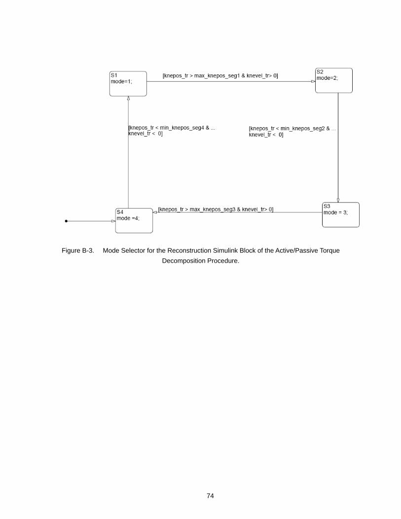
74

Figure B-3. Mode Selector for the Reconstruction Simulink Block of the Active/Passive Torque Decomposition Procedure.