1

NEW YORK UNIVERSITY

Urban Soundscape

Acoustic Event Classification

by

Zhiyuan Lin

Submitted in partial fulfillment of the requirements for the Master of Music in

Music Technology in the Department of Music and Performing Arts Professions in

The Steinhardt School New York University

Advisor: Tae Hong Park

[DATE: 2015/06/19] June 2015

2

NEW YORK UNIVERSITY

Abstract

Steinhardt

Master of Music

by Zhiyuan Lin

Automatic urban soundscape classification is an emerging research field

that has in recent years become an area of study and exploration along

with Big Data science. This field has its roots in acoustic ecology and

soundscape studies and at the same time, has interesting practical

possibilities. For example, Soundscape Information Retrieval (SIR)

[ICMC 2014 paper on SIR] can provide city managers cyber-physical

platforms to respond and address emergency response situations, noise

feedback, as well as other areas of urban management that have

important significance. This paper aims to try different methods to

achieve the pursuit of automated real-time soundscape classification.

The main research method is artificial neural networks and deep

learning. The focus on this thesis aims to do explore machine learning

and SIR without utilizing engineered salient features like MFCCs or

spectral centroids. Rather, we aim to directly use raw spectral

information computed from soundscape recordings. We utilized the

Citygram soundscape database to train and develop the prototype model.

3

Acknowledgements

I would like to thank Professor Tae Hong Park for his guidance, and

Professor Juan Bello saved me from confusion. They

both encourage d me and pointed out the way forward for me. And

Xiang Zhang, whom guide me into the field of machine learning, is not

only is a good friend, but a good teacher. Many people helped me solve

the problem of English. These include Huilin Pan, Eric Zhang and

Samuel Mindlin. Of course, I thank my parents for their financial

support. There are countless people who encouraged me and support me,

I will not forget.

4

Contents

1 Introduction ...................................................................................................................... 7

2 Prior work ...................................................................................................................... 10

2.1 CityGram ................................................................................................................. 10

2.2 Machine Learning ................................................................................................... 11

3 Dataset creation .............................................................................................................. 16

3.1 Data from CityGram Project ................................................................................... 16

3.2 Phase 1: Semi-manual sorting data and ground truth .............................................. 18

3.3 Phase 2: Data Preprocessing ................................................................................... 20

3.4 Phase 3: Principal Component Analysis (PCA) ..................................................... 23

3.5 Phase 4: Training, Verification, and Testing ........................................................... 24

4 Neural network training ................................................................................................. 25

4.1 Sparse Auto-encoder ............................................................................................... 25

4.2 Back Propagation .................................................................................................... 28

4.3 Conjugate Gradient Optimization ........................................................................... 29

5 Reliability Verification................................................................................................... 31

5.1 The control group data creation .............................................................................. 31

5.2 Structures an artificial neural network .................................................................... 32

5.3 The control group result .......................................................................................... 36

6 Training and Result ........................................................................................................ 39

6.1 Training ................................................................................................................... 39

6.2 Result ...................................................................................................................... 40

7 Conclusions and Future Work ........................................................................................ 47

7.1 Conclusions ............................................................................................................. 47

7.2 Future Work ............................................................................................................ 48

5

List of Figures

Figure 1 CityGram artificial acoustic event mark page .....................................17

Figure 2 audio cutting ........................................................................................21

Figure 3 The auto-encoder layout [Andrew Ng, Jiquan Ngiam, Chuan Yu Foo,

Yifan Mai, Caroline Suen. 2013] ...............................................................26

Figure 4 optimization algorithms for sparse auto-encoder [ Le, Q. V., et al.

2011] ..........................................................................................................30

Figure 5 lambda-cost curve ...............................................................................35

Figure 6 Distribution matrix results of experimental group ..............................41

Figure 7 Distribution matrix results of smaller network 1 ................................42

Figure 8 Distribution matrix results of smaller network 2 ................................43

Figure 9 Accuracy over varying number of Mel filters. ....................................45

6

List of Tables

Table 1 The training category ............................................................................18

Table 2 The architecture and results of 6-layer network ...................................33

Table 3 The architecture and results of 7-layer sparse auto-encoder ................33

Table 4 The testing accuracy of different sample length and segment

combinations ..............................................................................................34

Table 5 The iteration of training ........................................................................36

Table 6 The control group training result ..........................................................36

Table 7 The control group testing result ............................................................37

Table 8 The architecture of training network ....................................................39

Table 9 The results of experimental group ........................................................40

Table 10 The results of two control groups .......................................................42

Table 11 The architecture of two smaller network 1&2 ....................................43

Table 12 The results of two smaller network 1&2 ............................................44

7

1 Introduction

Although in the field of music information retrieval (MIR) and

soundscape information retrieval (SIR) [1Park, T. H., Lee, J. H., You, J.,

Yoo, M. J., & Turner, J. 2014], identification of sound has had a lot of

prior work, the research into urban soundscape classification still

remains scarce. Now people use voice commands to control mobile

phones, home appliances and even used to unlock the security lock. But

the common features of these sounds are precise targets and a single

generating source. Different from these, the composition of the urban

soundscape is complex and more difficult to predict. A lot of the objects

sound at the same time, and it is hard to distinguish noise from useful

information. Determined by the characteristics, urban sound is more

suited to a fuzzy algorithm. For a long time, researchers rely on a variety

of sound features, like Mel-frequency Cepstral Coefficients (MFCC)

(also, write Mel-frequency Cepstral Coefficients before abbreviating)

[2T. Ganchev, N. Fakotakis, and G. Kokkinakis 2005]. The feature and

the associated algorithm work well in certain situations. But for urban

sound field, rules needed for classification increase exponentially, and

the generalization power of a small number of features is small [3Jean-

Julien Aucouturier, Boris Defreville, and François Pachet. 2007]. To

8

engineer and specify rules is obviously very tedious work. There are no

specific rules within the network. The machine determines the rules, and

the practical efficiency of a well-trained artificial neural network is very

high. It makes decisions fast, and can be used in real-time systems. One

branch of machine learning, artificial neural network, can be considered

a bionics computing architecture. Prior to this, researches on artificial

neural networks have been numerous. But most of them still use

conventional audio features. However, we know that most of the

features are not invertible after signal decomposition. It means that after

compression, some audio information will be lost. Since computing

power is so advanced today, we can try to process raw data. In the case

of less compression, the accuracy and generalization of sound

classification is expected to increase. This thesis involves an experiment

on the direct use of audio for urban soundscape classification.

This thesis is a subproject of CityGram. Utilzing Citygram soundscape

dataset for this research saved a lot of time that would have been spent

on data collection. At the same time, many predecessors are important

references for this research, including the work of a former

“Citygrammer” and former Music Technology student at NYU. Many

parameters of this study largely made reference to previous experience

[4Jacoby. 2014].

9

10

2 Prior Work

A soundscape is a sound or combination of sounds that forms or arises

from an immersive environment [5Retrieved from Wikepedia]. The

sound of urban soundscape mostly generated by human activities

[6Raimbault, M., & Dubois, D. 2005]. There is a lot of theoretical

research on urban soundscapes, but most lack the involvement of

automatic scientific tools. In this regard, Citygram is one of the few big

city data research projects. When introducing the CityGram project, we

also need to include some background about machine learning.

2.1 CityGram

CityGram is a large-scale urban sound data collection and analysis

project. In 2011, the Citygram Project in its first iteration was launched

to develop dynamic non-ocular energy maps focusing on acoustic

energy [7Park, T. H., Lee, J. H., You, J., Yoo, M. J., & Turner, J. 2014].

Through the Remote Sensing Devices (RSD) installed or dispersed

throughout the city, it collects the city's sound and generates a regional

soundscape. Researchers will be able to have access to real-time audio

11

and audio feature information through the Citygram server. One group

within CityGram is working on automated soundscape classification

through the database of artificial markings of acoustic events in audio.

More research will be launched in the future.

2.2 Machine Learning

Now, neural networks and support vector machines are two kinds of

representative statistical learning methods of machine learning. They

can be considered derived from linear classification models (Perceptron)

Rosenblatt invented in 1958. Perceptron only performs linear

classification [8Freund, Y.; Schapire, R. E. 1999], but in reality the

problem is usually non-linear. Neural Networks and Support Vector s are

non-linear classification models. In 1986, Rumelhart and McClelland

invented the Back Propagation algorithm. This algorithm is an important

form of supervised learning, also used in this experiment. Later, Vapnik

et al proposed SVM in 1992 [9Bottou, L., & Vapnik, V. 1992]. A neural

network is a multi-layer (usually three) non-linear model; use a vector

machine to convert the nonlinear problem into a linear problem. For

Personal computer, the training of artificial neural networks takes very

long, while SVM no small advantage in this regard. Therefore, SVM has

been widely used in the industry for a very long time [10Suykens, J. A.,

12

& Vandewalle, J. 1999]. However, with the advances in theory and

hardware performance, artificial neural networks once again

demonstrated its capabilities.

2.2.1 Artificial Neural Network

Artificial neural networks (ANNs) are a family of statistical learning

models, Inspired by biological neural network. The network itself does

not store data, nor manually define things, but the network functions

through training and recording of the neuronal node reaction to the input

data. Artificial neural networks typically have multiple layers of

interconnected neurons. The bottom layer is the input layer, and is

responsible for receiving external stimuli. The layers in the middle are

called the hidden layers. Similar to the biological process of neuronal

cells, the information is passed up layer by layer. This process is similar

to the human brain patterns of induction, generalization and analysis.

Finally at the highest level or the output layer, the network has the

ability to perceive and classify. For example, in the field of image

recognition, the colors and coordinates of the pixels in the picture will

be used as the input layer. Lower layers can sum up and describe the

lines and edges in the picture. Higher layers can construct simple shapes

together with lines and edges [11Duygulu, P., Barnard, K., de Freitas, J.

13

F., & Forsyth, D. A. 2002]. Finally, the highest level can identify the

object.

In the audio field, the human ear can perceive frequency, intensity, and

duration [12Gaskill, S. A., & Brown, A. M. 1990]. A short time Fourier

transform spectrum can reflect these three dimensions, while its data

structure is also similar to a picture. Therefore, we assume that these

multilayer neural networks can simulate the human perception of sound,

thus achieving the acoustic event classification purposes.

The neural networks must be trained first before using artificial neural

networks, and training is an iterative process. Before 2006, a typical

artificial neural network would utilize back propagation method with

adjustable parameters. Typically, the neuronal node parameters of the

network will be initialized with a random number. During the iterations,

network will input the existing data set, and the network will give

recognition results for all samples in output layer. The ground truth is

compared to the output layer of the network, and an offset parameter is

calculated and passed from the output layer back to the lower layer

[13Mason, L., Baxter, J., Bartlett, P., & Frean, M. 1999]. In the next

iteration, the node parameters use the result of the previous iteration.

When this process is repeated, the recognition results of the network

will gradually move closer to the ground truth. After the training is

14

completed, the network will have the ability to classify new samples.

2.2.2 Deep Learning

Compared to the brain, the number of neurons on artificial neural

network is still very small [14Jain, A. K., Mao, J., & Mohiuddin, K. M.

1996]. Moreover, the number of connections between neurons in the

human brain is more complex and diverse. Therefore, in the field of

machine learning, achieving a high level of perception with a small

number of neuronal connections is very difficult. We naturally think of

increasing the number of layers and nodes of artificial neural networks.

But when the number of layers is large, the offset value generated from

the output layer becomes very small. This makes the training to stop at

one stage. In 2006, Hinton proposed Deep Belief Networks that greatly

enhance the ability of neural networks. His approach is, for a multi-

ANN, first with Boltzmann Machine (unsupervised learning) structure

learning networks, and then through the weighted Back Propagation

(supervised learning) Learning Network [15Hinton, G. E., 2006]. Today,

the use of artificial neural networks for image recognition has made

great breakthroughs. The original intention of this thesis is to transplant

a method of image classification to sound classification, so as to explore

the performance of deep learning classification.

15

16

3 Dataset Creation

Similar to the mechanism of how humans discern sounds, supervised

machine learning requires that the machine listens to adequate volumes

of audio samples and is given the category to which each audio sample

belongs. Each audio sample that the machine listens to requires

descriptions provided by a human. It would be a huge project for one

researcher to label many audio profiles. Therefore, Citygram Database,

built by multiple researchers, and multiple annotators (up to 7 per

soundscape recording at present time), holds the date and time of

acoustic events and other details. Though humans are subjective in

describing things and events, especially for sounds, the results of the

supervised machine learning project rely extensively upon the quality of

the samples and quality to the ground truth. To be specific, we

normalized the audio sample descriptions from each individual

researcher.

3.1 Data from CityGram Project

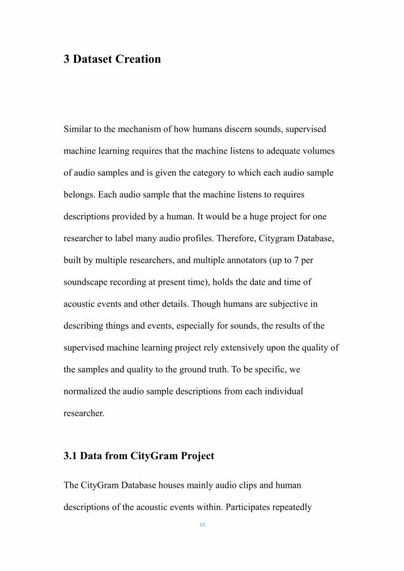
The CityGram Database houses mainly audio clips and human

descriptions of the acoustic events within. Participates repeatedly

17

listened to audio sample in 2-minute segment durations to extract

meaningful acoustic events and provide descriptions. They set the start

and end time of the acoustic events, gave verbal descriptions of the

acoustic events, and assessed the distance of the source of the sound and

other attributes based on personal judgment.

Figure 1 CityGram artificial acoustic event mark page

Urban soundscapes are noisy [16Park, T. H., Lee, J. H., You, J., Yoo, M.

J., & Turner, J. 2014]. However, there is no good normalization on the

verbal descriptions, as different people have different language

preferences. For example, some people would use "walking" while some

others would use "footprint". Some labels differentiate the origins of the

sound, such as "men's voice" from "female speaking", while some

others would simply categorize it as "human sound."

In the training step of supervised machine learning, each category

18

demands a certain number of samples. If we discerned sounds in great

detail, we would have too many categories and too few samples in each

category. Thus, it was necessary to merge some categories.

3.2 Phase 1: Semi-manual Sorting Data and Ground Truth

There were more than 1,700 acoustic events. It would have been

inefficient to manually categorize them. We employed the original data

from the CityGram database server, and then looked them up in

Microsoft Excel with the Fuzzy Lookup plugin.

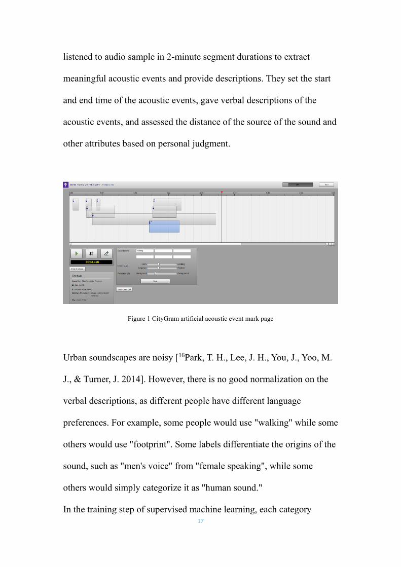
According to the description of the sample and their numbers in

database, we chose the following nine classes:

1 2 3 4 5 6 7 8 9

walking vehicle engine horn background machine quiet music speech

Table 1 The training category

Basically, “Walking” means the sound of a human walking. The

difference between “vehicle” and “engine” is that “engine” refers

specifically to the sound of the engine and the motor, and “vehicle”

usually refers to the passing sound of vehicles. “Machine” includes

19

various types of percussion. “Music” refers specifically to melodic

sound, not including percussion. The last category, “speech” includes all

kind of human voices, like laughing or yelling. “Quiet” is a special

class, which includes a large number of audio clips that are not marked.

It is not considered significant, and can be treated as silence.

There are several keywords under each category, such as "walking",

"walk", and "footstep" under the category, "walking". Fuzzy Lookup

checked each record of data against the keywords in the category, and

gave a resemblance score. Based on the resemblance scores, we had one

more manual check, and eliminated incorrect categorizations and

duplicate labels. During the manual check, we also added data without

keywords. In the end, there were around 1,200 acoustic events for the

training of supervised machine learning. Refer to audio clips, it is about

2 hours in total.

This classification reference to previous experience, but also taking into

account the limitations of the database itself [17Justin Salamon,

Christopher Jacoby, Juan Pablo Bello., 2014]. The core idea is separate

the sound into four categories: human, nature, machinery and music.

However, 50% of the label in database belong to human. It means that

even all judges are human, it is still close to 50% recognition accuracy

rate. In order to balance gravity, we subdivided several classes to give

20

the final categories. In the process of breakdown, we also considered

some of the spectral characteristics of the sound, such as percussion in

music. Even if it has a bit of a unique rhythm, the length of percussion

samples less than 3 minutes. Such a small sample size is difficult to

extract a sound concept. So I attributed it to the category of the machine

with other beating, striking sound. In short, such categories are not

based on generic classification, but customized according to existing

resources. Algorithm itself is generic, and does not consider any special

factors of sound sample.

3.3 Phase 2: Data Preprocessing

Because our artificial neural network was run in MATLAB, we also

used MATLAB to preprocess original data. Data loaded into MATLAB,

and cut into pieces from the original audio based on the start time and

end time in the SQL databas.

3.3.1 Windowing

During extraction of acoustic events, deviations could arise with

different choice of timeline segregation. In fact, we sometimes found it

hard to distinguish a meaningful acoustic event from background noises.

21

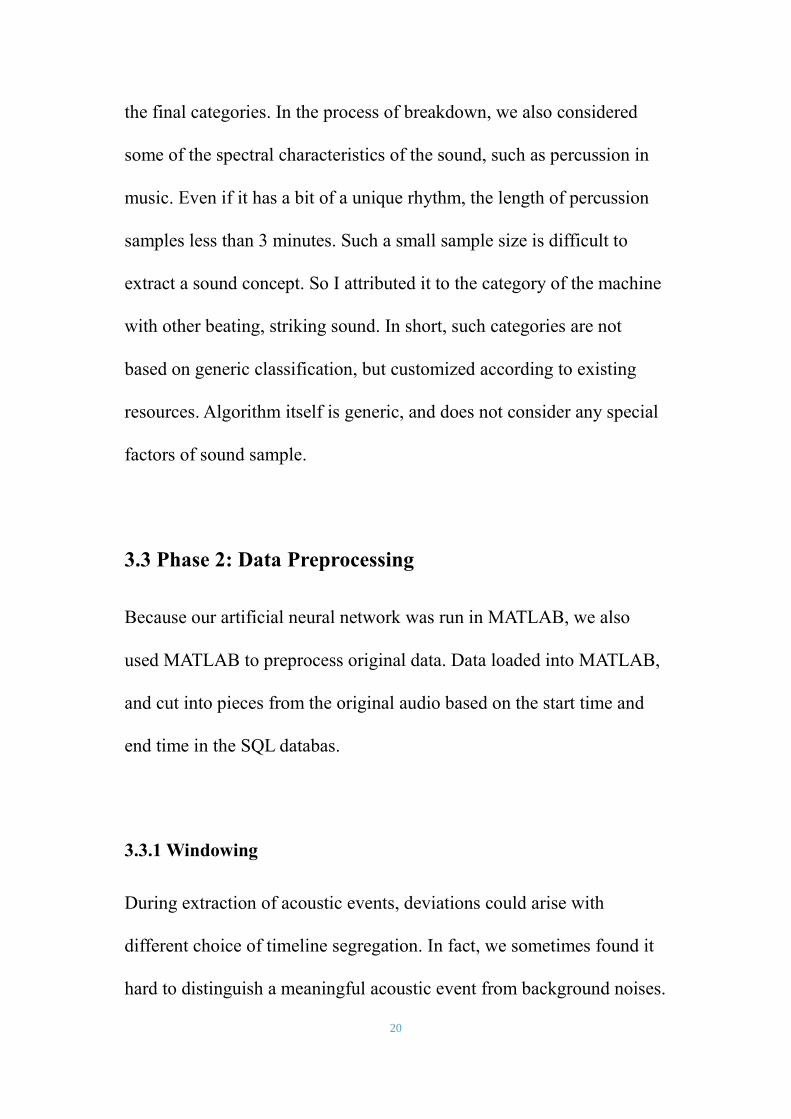
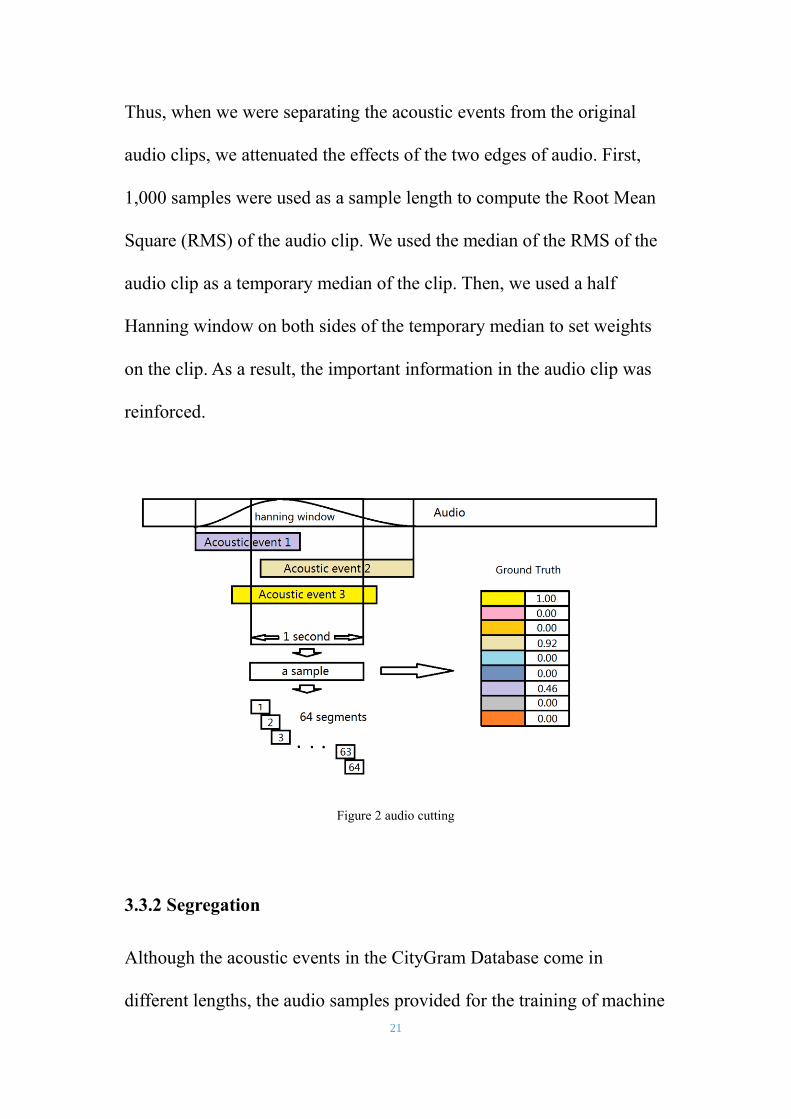
Thus, when we were separating the acoustic events from the original

audio clips, we attenuated the effects of the two edges of audio. First,

1,000 samples were used as a sample length to compute the Root Mean

Square (RMS) of the audio clip. We used the median of the RMS of the

audio clip as a temporary median of the clip. Then, we used a half

Hanning window on both sides of the temporary median to set weights

on the clip. As a result, the important information in the audio clip was

reinforced.

Figure 2 audio cutting

3.3.2 Segregation

Although the acoustic events in the CityGram Database come in

different lengths, the audio samples provided for the training of machine

22

learning model must be of the same length, and thus we had to trim

some of the input data. In reality, common people do not need to listen

to the entire acoustic event to discern the category of the sound. For

example, under the category of “voices”, common people only need to

hear a word, instead of a whole conversation or paragraph, to tell if that

is someone talking. Therefore, a long human conversation could be

deemed as an aggregation of multiple samples in the “voices” category.

In the data preprocessing stage, we tried 3 sample lengths - 1-second, 2-

seconds, and 4-seconds. For the 1-second length, we separated an

acoustic event into multiple overlapping1-second clips; and clips shorter

than 1 second were zero padded. After the training, we examined how

samples with different lengths could affect the results. After the training,

we examined how samples with different lengths could affect the

results.

On the other hand, the ground truth of each sample was decided by the

ratio of the category among the sample. For example, if half of the

sample is human voice, the ground truth of “speech” is 0.5. Therefore,

the ground truth of each sample is an array of 9 numbers between 0 and

1, each of which corresponds to the pre-defined category.

Then, taking samples of 1-second as example, in order to show that the

spectrum within the samples changes with time, we needed to perform a

23

second segregation on the samples. Each sample was separated into 64

segments with overlap. Each of the 64 segments were then transformed

with the Fast Fourier Transform (FFT), yielding 64*n*2 rough samples,

in which n refers to the number of samples in each segment and 2 refers

real and imaginary. Each sample includes the real and complex part of

the 64 segments after FFT.

3.4 Phase 3: Principal Component Analysis (PCA)

If data with little or no preprocessing were used for machine learning,

the input number would be too large (i.e. n > 20,000). In order to run our

neural network on a personal computer, we needed to reduce the

dimensions, and thus we employed Principal Component Analysis

(PCA). PCA uses fewer dimensions to describe a higher dimensional

data, although some information might be lost [18Barnett, T. P., and R.

Preisendorfer. 1987]. However, the PCA computation consumes a high

amount of memory and CPU. To lift the heavy burden of computing, we

computed all the data within each segment repeatedly 64 times, instead

of computing all the data within the 64 segments all together. For

reasons of computing power, we only selected features include 98% of

the information. The number of features of each segment ranging

between 35 and 90. Finally, they were combined into a single dataset.

24

3.5 Phase 4: Training, Verification, and Testing

In Machine Learning, data samples are usually divided into three

groups, among which the largest is used for training and another is for

verification. The method of using a group of data for verification is

called Cross Validation. Observing the results of Cross Verification can

help us revise the coefficients of neural network, resulting in better

training results [19Krogh, A., & Vedelsby, J. 1995]. However, to prevent

over-fitting, we need the test group for final examination of neural

network. To take 1-second samples for example, there were around

5,600 samples in the end, among which 3,600 were used for training,

1,000 for verification, and the other 1,000 for testing. In the process of

grouping, we conducted two randomized sort. The first time, all of the

original audio is randomly ordered, according to the length of time to be

roughly assigned to three groups. This ensures that the audio source of

three groups are completely separate. The second time, after completion

of the cutting, sample set is randomly ordered again for pretreatment. A

predictable disadvantage is that there will be two sample from the same

audio clip. In addition, during the cutting process, the sample itself is

overlapping, somewhat lower the quality of samples. Given the limited

25

number of artificial labels, this is a compromise choice.

4 Neural Network Training

This experiment used a sparse auto-encoder neural network. When

building an artificial neural network, we first pre-train each layer using a

sparse auto-encoder. Then parameters are adjusted with back

propagation algorithm.

4.1 Sparse Auto-encoder

The sparse auto-encoder is relatively well known in the field of Deep

learning, which is a method of unsupervised learning [20Bengio,

Y.2009]. It is essentially a three-layer neural network, an input layer,

output layer and a hidden layer. Unlike common shallow neural

network, ground truth of its output layer is the input layer data. Its

significance lies in the hidden layer that can better reconstruct the input

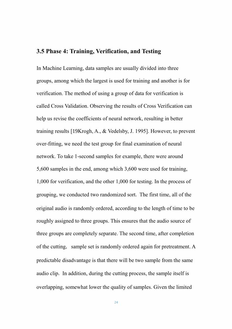
layer information. As shown in figure:

26

Figure 3 The auto-encoder layout [21Andrew Ng, Jiquan Ngiam, Chuan Yu Foo, Yifan Mai, Caroline

Suen. 2013]

This is a simple auto-encoder, its cost function formula is:

Where J is the cost, m is the amount of samples, l is the number of layer

and the lambda is the regularization parameter. When J is 0, it indicates

that the network can be 100 percent accurate in reproducing the original

data. But this situation is too extreme, and prone to over-fitting. If the

training of a network appears to be over-fitting, it can only perform very

27

well in training data set, but fail to generalize to new samples [5Andrew

Ng, Jiquan Ngiam, Chuan Yu Foo, Yifan Mai, Caroline Suen. 2013].

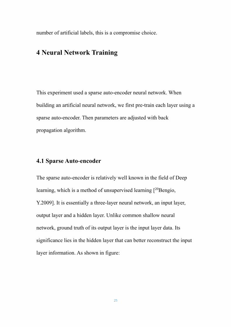
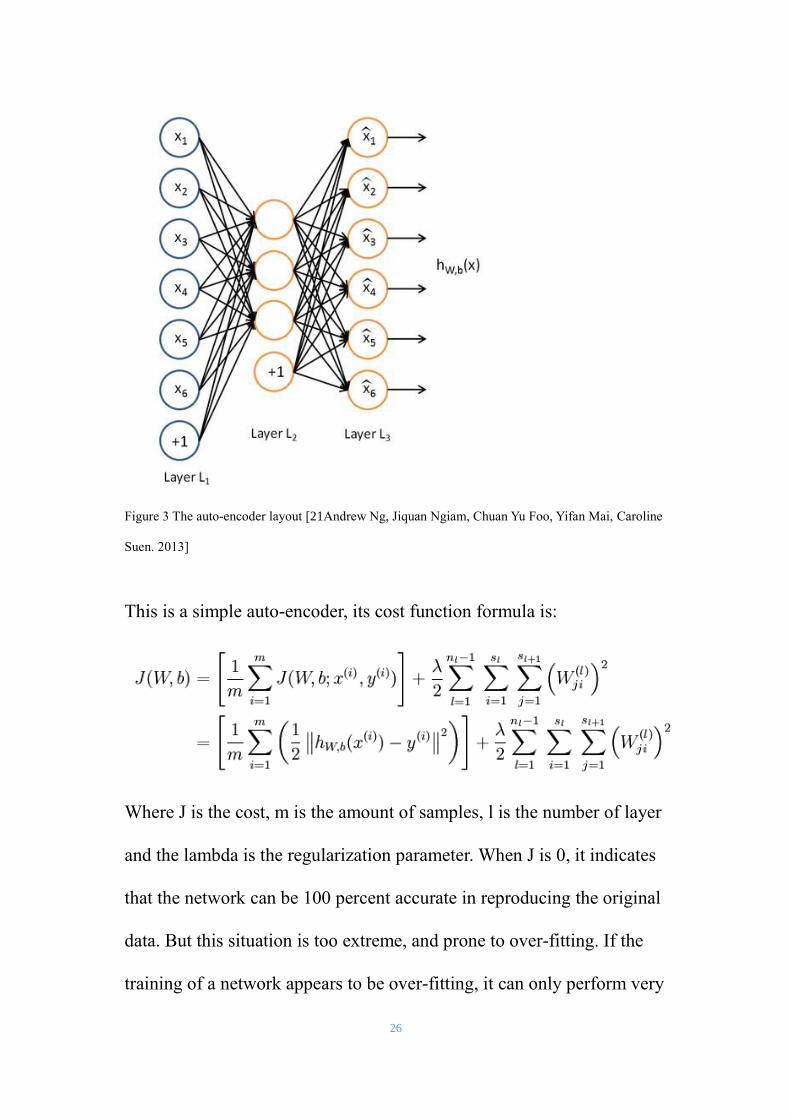
Adding sparse coding is a way place constraints on output layers, so

only the more important nodes are activated, and most of the hidden

layer nodes are in a non-active state. This will achieve the purpose of

sparse coding. Therefore, the sparse auto-encoder cost function

expression is:

𝐽𝑠𝑝𝑎𝑟𝑠𝑒(𝑊, 𝑏) = 𝐽(𝑊, 𝑏) + 𝛽 ∑ 𝐾𝐿(𝜌||𝜌�̂�)

𝑠2

𝑗=1

The new item that is Kullback-Leibler (KL) distance, which is expressed

as follows:

𝐾𝐿(𝜌||𝜌�̂�) = 𝜌 log𝜌

𝜌�̂�+ (1 − 𝜌) log

1 − 𝜌

1 − 𝜌�̂�

The hidden layer node average output is calculated as follows:

𝜌�̂� = 1

𝑚 ∑[𝑎𝑗

(2)(𝑥(𝑖))]

𝑚

𝑖=1

Where the parameter ρ is generally small, such as 0.05, which means

that there is a small probability of the event occurring. The probability

of each hidden layer node being activated approaches 0.05 [5Andrew

Ng, Jiquan Ngiam, Chuan Yu Foo, Yifan Mai, Caroline Suen. 2013].

The auto-encoder with the sparseness usually performs better

28

[22Marc’Aurelio Ranzato, Christopher Poultney, Sumit Chopra and Yann

LeCun. 2006]. It enhances the outstanding feature, and weakened other

features.

4.2 Back Propagation

After the methods above, we can build the multi-layer structure that we

want. However, we still lack a scientific way to evaluate the number of

layers needed and the number of neuronal nodes in each layer. The

neural network is now able to reconstruct original data well, but it does

not yet known how to classify. Next, in order to add an additional output

layer onto the top layer of the neural network, we can use a standard

method of training: back propagation. In this thesis we use gradient

descent method for back propagation. This process is like using a

specific length of pace to find the lowest point down along the path [23

Rumelhart, David E.; Hinton, Geoffrey E.; Williams, Ronald J. 1986]. It

transforms an issue of the lowest point calculation to an issue that can be

calculated by successive approximation. But we need to choose the

appropriate test steps, so that it will not miss the target concave point or

explore too slowly. The cost function formula is:

𝐽 = [1

2𝑚∑ ∑(|ℎ𝑖𝑖 − 𝑦𝑖𝑗|2)

𝑐

𝑗=1

𝑚

𝑖=1

] +𝜆

2𝑚∑ ∑ ∑(𝑊𝑖𝑗

(𝑙))2

𝑐

𝑗=1

𝑚

𝑖=1

𝑛−1

𝑙=1

29

Where m is the number of samples, c is the number of categories

and n is the number of layers.

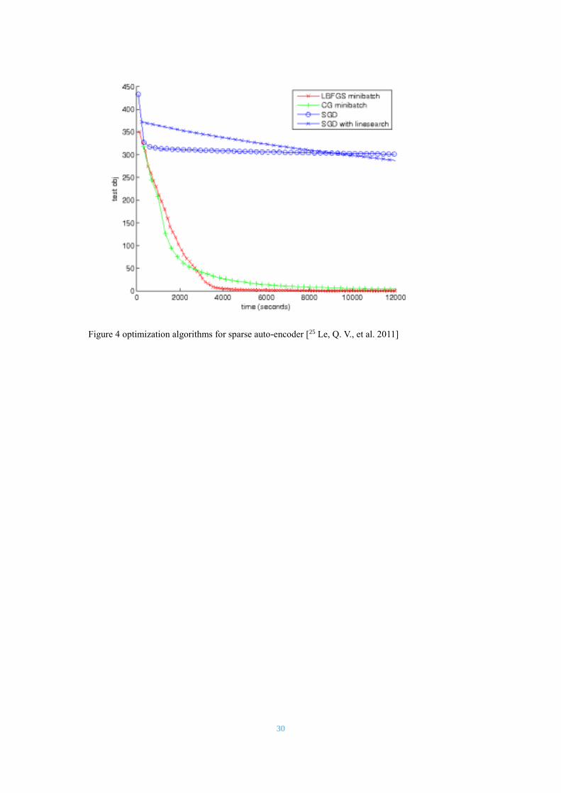
4.3 Conjugate Gradient Optimization

As mentioned above, the network training will be an iterative process.

To use MATLAB to iterate, while a viable approach, does not achieve

high efficiency. In the experiment, we use conjugate gradient as our

optimization algorithm. The conjugate gradient optimization is a

numerical solution usually for a large sparse system [24

Hestenes, Magnus R.; Stiefel, Eduard 1952]. It can make the cost of

network decline faster than ordinary gradient descent. For sparse auto-

encoder network, performances of several optimization algorithms

showed as below:

30

Figure 4 optimization algorithms for sparse auto-encoder [25 Le, Q. V., et al. 2011]

31

5 Reliability Verification

It is well known that the urban soundscape is an inherently noisy

environment. While in the street, to hear the sound of car horns and the

sound of the engine is a very common thing. This kind of classification

is difficult to guarantee to be completely correct, even for a human. If

we use existing experimental data directly, we will lack an effective

control group. It may be difficult to judge whether the defects of the

system come from noise and diverse spectrum or from the system itself.

Since training the neural network takes a very long time, we have to first

verify the reliability of the system. The following experiment is the

control group.

5.1 The Control Group Data Creation

The data preprocessing of the control group and the experimental group

is exactly the same, the only difference being their data. The control

group audio consists of several common instrument solos. A solo is

characterized by a small noise and no confounding acoustic event. Only

one instrument sounds at any particular time. Using instrument solos as

32

a control group can test feasibility and sound classifier performance. We

selected a total of 34 solo sounds divided into four classes. There were

15 piano songs, 11 violin songs, 7 guitar songs and 20 minutes of mute

background with the device noise as the silent group. Solo samples are

from different styles and periods, and they had silence removed. Most of

them are from classical music sources. Cutting and pretreatment resulted

in a total of 2800 samples, 1 second long per sample。After shuffling,

1800 of them were used to train, 500 were used to validation and 500 for

testing.

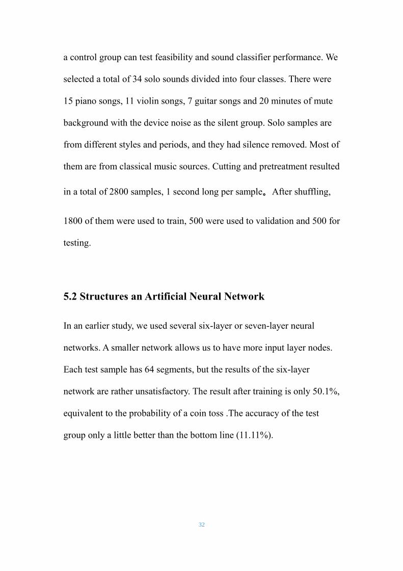
5.2 Structures an Artificial Neural Network

In an earlier study, we used several six-layer or seven-layer neural

networks. A smaller network allows us to have more input layer nodes.

Each test sample has 64 segments, but the results of the six-layer

network are rather unsatisfactory. The result after training is only 50.1%,

equivalent to the probability of a coin toss .The accuracy of the test

group only a little better than the bottom line (11.11%).

33

layer input 2 3 4 5 output

Number of nodes 5696 4096 4096 4096 4096 4

Training accuracy 50.1%

Testing accuracy 33.70%

Table 2 The architecture and results of 6-layer network (1 second sample length, 64 segments per

sample, lambda = 3, iteration: 50)

The results of 7-layer network are not much better than that of the 6-

layer network.

layer input 2 3 4 5 6 output

number of nodes 5696 4096 4096 4096 4096 4096 4

training accuracy 72.2%

testing accuracy 51.27%

Table 3 The architecture and results of 7-layer sparse auto-encoder (1 second sample length, 64

segments per sample, lambda = 3, iteration: 50)

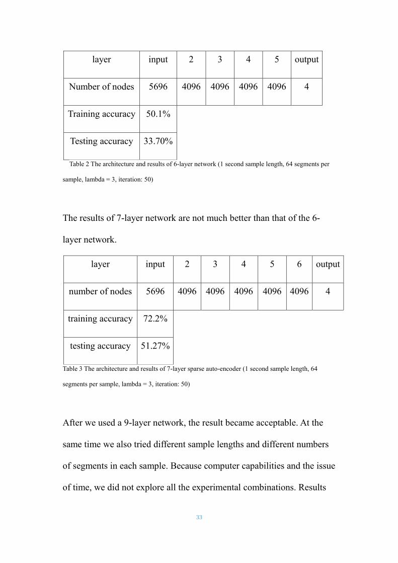
After we used a 9-layer network, the result became acceptable. At the

same time we also tried different sample lengths and different numbers

of segments in each sample. Because computer capabilities and the issue

of time, we did not explore all the experimental combinations. Results

34

are shown below:

segment/length 1s 1.5s 2s 4s

16 51.16% 52.34% 51.34% 34.65%

32 51.16% 56.63% 46.46% 42.50%

64 72.57% 51.64% 52.48% 66.64%

128 N/A 70.98% 21.85% N/A

256 N/A N/A 61.48% N/A

Table 4 The testing accuracy of different sample length and segment combinations (lambda =3,

iteration: 50)

Although not very obvious, more segments and a short time obtained

better results. This experiment did not give us much reference, since

different sample lengths can lead to large changes in the experimental

samples. And the number of samples is relatively small, which means

the randomness of the results is relatively large.

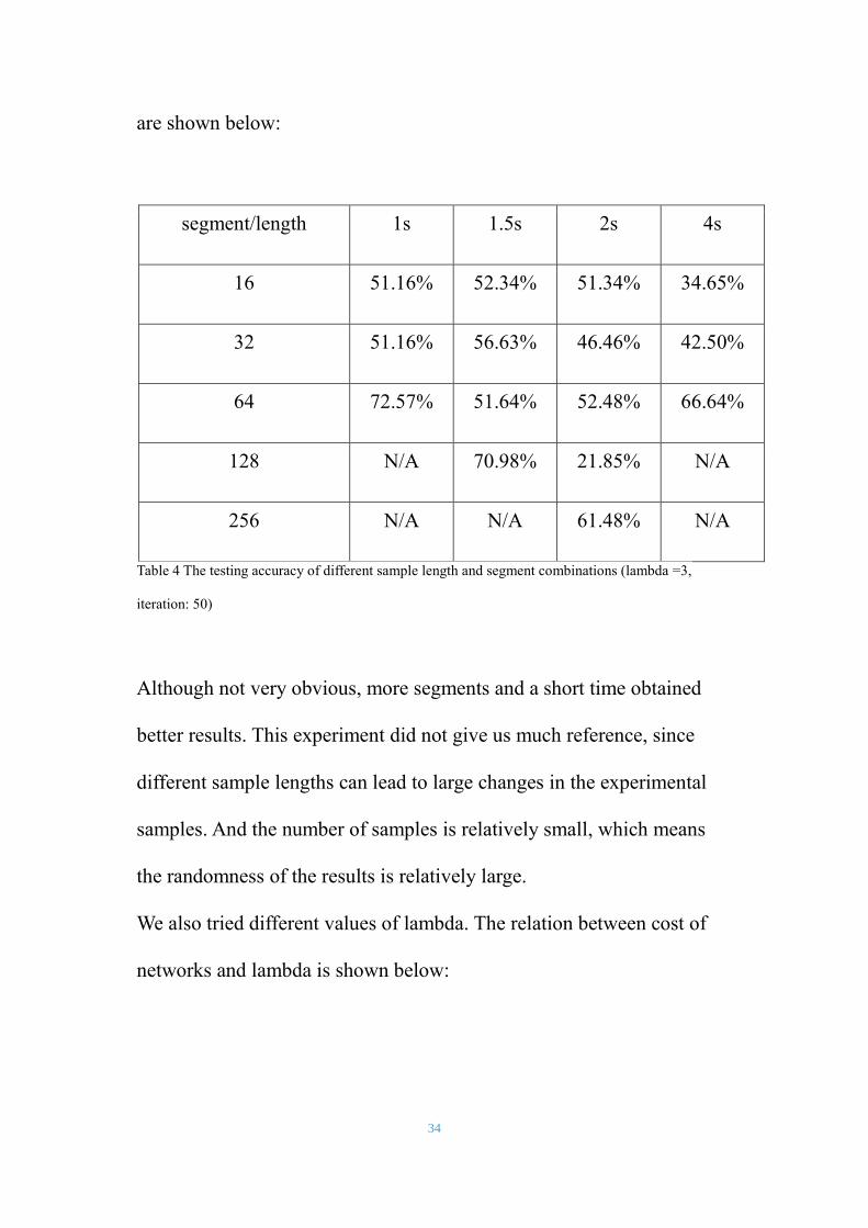
We also tried different values of lambda. The relation between cost of

networks and lambda is shown below:

35

Figure 5 lambda-cost curve (1 second sample length, 64 segments per sample, iteration: 50)

The green curve is the validation set, and the blue curve is the training

group. As shown in figure, the validation group did not reach the

inflection point. This means the network is still in an under-fitting state.

The number of nodes in the artificial neural network is not enough to

summarize and describe the input data [26M. Ranzato, C. Poultney, S.

Chopra, and Y. LeCun. 2007].

In addition, we also tried to change the different auto-encoder training

iterations. Too few iterations may cause unfitting, contrary, too many

iterations may cause overfitting [S. Amari, N. Murata, K. -R. Muller, M.

Finke, H. H. Yang 1997]. Both of them are 27not good situations for

36

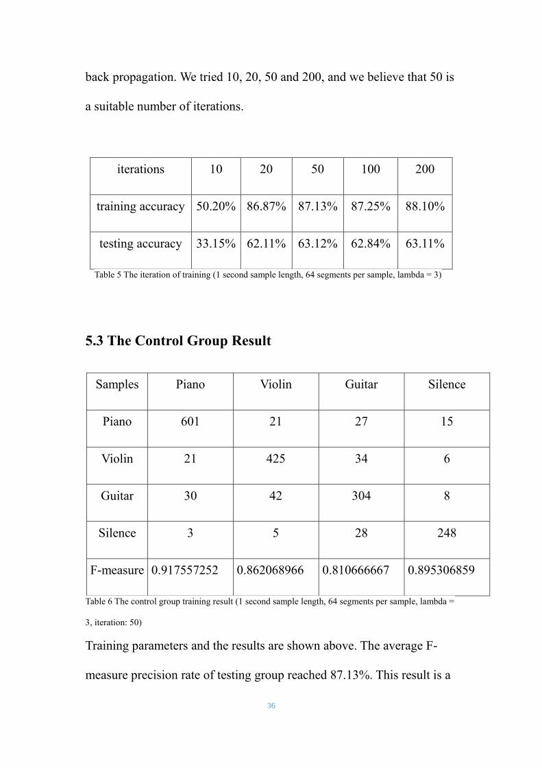
back propagation. We tried 10, 20, 50 and 200, and we believe that 50 is

a suitable number of iterations.

iterations 10 20 50 100 200

training accuracy 50.20% 86.87% 87.13% 87.25% 88.10%

testing accuracy 33.15% 62.11% 63.12% 62.84% 63.11%

Table 5 The iteration of training (1 second sample length, 64 segments per sample, lambda = 3)

5.3 The Control Group Result

Samples Piano Violin Guitar Silence

Piano 601 21 27 15

Violin 21 425 34 6

Guitar 30 42 304 8

Silence 3 5 28 248

F-measure 0.917557252 0.862068966 0.810666667 0.895306859

Table 6 The control group training result (1 second sample length, 64 segments per sample, lambda =

3, iteration: 50)

Training parameters and the results are shown above. The average F-

measure precision rate of testing group reached 87.13%. This result is a

37

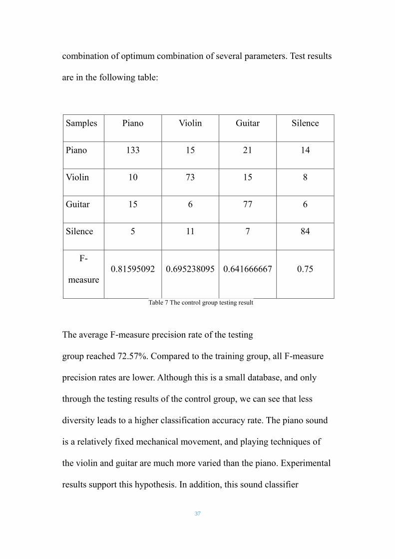
combination of optimum combination of several parameters. Test results

are in the following table:

Samples Piano Violin Guitar Silence

Piano 133 15 21 14

Violin 10 73 15 8

Guitar 15 6 77 6

Silence 5 11 7 84

F-

measure

0.81595092 0.695238095 0.641666667 0.75

Table 7 The control group testing result

The average F-measure precision rate of the testing

group reached 72.57%. Compared to the training group, all F-measure

precision rates are lower. Although this is a small database, and only

through the testing results of the control group, we can see that less

diversity leads to a higher classification accuracy rate. The piano sound

is a relatively fixed mechanical movement, and playing techniques of

the violin and guitar are much more varied than the piano. Experimental

results support this hypothesis. In addition, this sound classifier

38

algorithm is shown to be feasible, though the accuracy needs to be

improved. It is worth noting that, since the number of audio samples is

limited, different parameters will change the number of samples. And

because the computer's memory limit, an excessive number of samples

will make the computer run out of memory. In the next step of training

we need to weigh the selection of parameters. More segments and a

longer sample length means fewer amount of samples. Before the results

came out, the choice was very difficult.

39

6 Training and Result

Although machine learning takes a long time, we conducted a number of

experiments including cross validation, and tried a variety of

parameters. Even not all of the experiments are successful, they give us

a good reference direction.

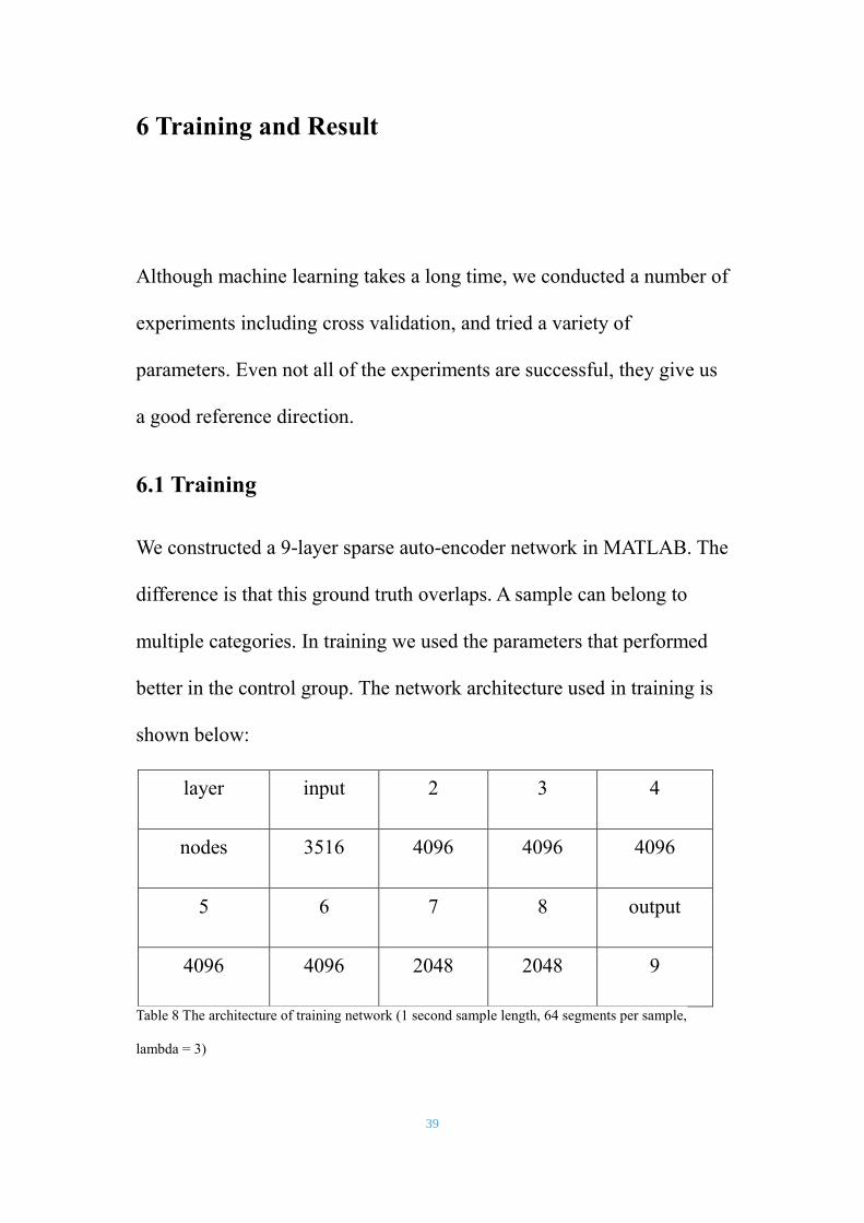
6.1 Training

We constructed a 9-layer sparse auto-encoder network in MATLAB. The

difference is that this ground truth overlaps. A sample can belong to

multiple categories. In training we used the parameters that performed

better in the control group. The network architecture used in training is

shown below:

layer input 2 3 4

nodes 3516 4096 4096 4096

5 6 7 8 output

4096 4096 2048 2048 9

Table 8 The architecture of training network (1 second sample length, 64 segments per sample,

lambda = 3)

40

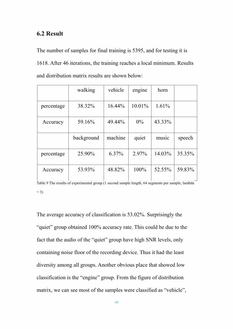
6.2 Result

The number of samples for final training is 5395, and for testing it is

1618. After 46 iterations, the training reaches a local minimum. Results

and distribution matrix results are shown below:

walking vehicle engine horn

percentage 38.32% 16.44% 10.01% 1.61%

Accuracy 59.16% 49.44% 0% 43.33%

background machine quiet music speech

percentage 25.90% 6.37% 2.97% 14.03% 35.35%

Accuracy 53.93% 48.82% 100% 52.55% 59.83%

Table 9 The results of experimental group (1 second sample length, 64 segments per sample, lambda

= 3)

The average accuracy of classification is 53.02%. Surprisingly the

“quiet” group obtained 100% accuracy rate. This could be due to the

fact that the audio of the “quiet” group have high SNR levels, only

containing noise floor of the recording device. Thus it had the least

diversity among all groups. Another obvious place that showed low

classification is the “engine” group. From the figure of distribution

matrix, we can see most of the samples were classified as “vehicle”,

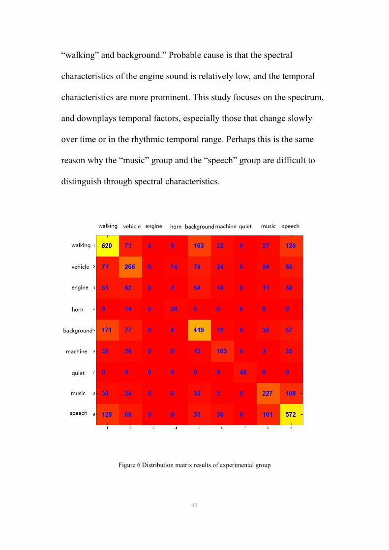
41

“walking” and background.” Probable cause is that the spectral

characteristics of the engine sound is relatively low, and the temporal

characteristics are more prominent. This study focuses on the spectrum,

and downplays temporal factors, especially those that change slowly

over time or in the rhythmic temporal range. Perhaps this is the same

reason why the “music” group and the “speech” group are difficult to

distinguish through spectral characteristics.

Figure 6 Distribution matrix results of experimental group

42

There are two control groups with less samples in training. The number

of samples for control group 1 training is 2600, and control group 2

training is 1300. Results and distribution matrix results are shown

below:

accuracy walking vehicle engine horn

Group 1 56.64% 44.72% 44.78% 43.10%

Group 2 35.28% 32.03% 29.39% 22.41%

background machine quiet music speech

Group 1 51.39% 45.95% 100% 52.71% 54.09%

Group 2 34.56% 14.40% 50% 34.21% 36.55%

Table 10 The results of two control groups (1 second sample length, 64 segments per sample, lambda

= 3)

The average accuracy of control group 1 is 52.95%, and the he average

accuracy of control group 2 is 33.88%. The group with more samples

have higher accuracy.

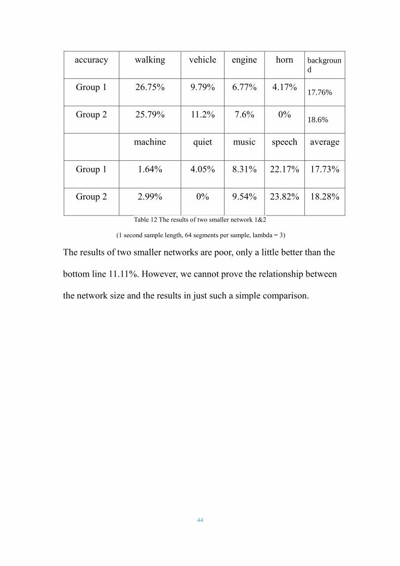
There are result of two control groups with smaller size of network.

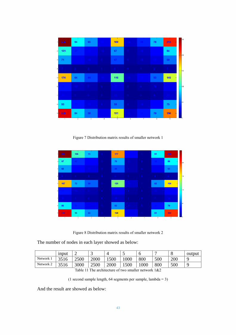
43

Figure 7 Distribution matrix results of smaller network 1

Figure 8 Distribution matrix results of smaller network 2

The number of nodes in each layer showed as below:

input 2 3 4 5 6 7 8 output Network 1 3516 2500 2000 1500 1000 800 500 200 9 Network 2 3516 3000 2500 2000 1500 1000 800 500 9

Table 11 The architecture of two smaller network 1&2

(1 second sample length, 64 segments per sample, lambda = 3)

And the result are showed as below:

44

accuracy walking vehicle engine horn backgroun

d

Group 1 26.75% 9.79% 6.77% 4.17% 17.76%

Group 2 25.79% 11.2% 7.6% 0% 18.6%

machine quiet music speech average

Group 1 1.64% 4.05% 8.31% 22.17% 17.73%

Group 2 2.99% 0% 9.54% 23.82% 18.28%

Table 12 The results of two smaller network 1&2

(1 second sample length, 64 segments per sample, lambda = 3)

The results of two smaller networks are poor, only a little better than the

bottom line 11.11%. However, we cannot prove the relationship between

the network size and the results in just such a simple comparison.

45

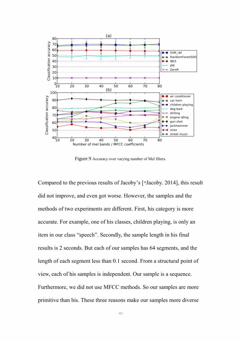
Figure 9 Accuracy over varying number of Mel filters.

Compared to the previous results of Jacoby’s [28Jacoby. 2014], this result

did not improve, and even got worse. However, the samples and the

methods of two experiments are different. First, his category is more

accurate. For example, one of his classes, children playing, is only an

item in our class “speech”. Secondly, the sample length in his final

results is 2 seconds. But each of our samples has 64 segments, and the

length of each segment less than 0.1 second. From a structural point of

view, each of his samples is independent. Our sample is a sequence.

Furthermore, we did not use MFCC methods. So our samples are more

primitive than his. These three reasons make our samples more diverse

46

in the frequency domain. Our advantage is that our network has better

generalization; the disadvantage is that such algorithm needs more

training samples.

47

7 Conclusions and Future Work

7.1 Conclusions

In this thesis, we tried a direct use of original audio spectrum for

machine learning in the analysis of urban soundscapes. We also tried to

use different audio pre-processing parameters, as well as different

number of samples. Its average classification accuracy reached 53.02%,

and the best individual classification accuracy reached 59.83% for a

total of 8 classes. Some results may consistent with the hypothesis: this

network has high bias problem, so an increase in the number of samples

can improve accuracy. But given the low accuracy of the results, we

cannot prove that the diversity of spectrum and number of samples are

completely relevant in urban soundscape acoustic event classification.

In this experiment, the deficiencies will be a lesson for future study. Due

to the characteristic urban sound, samples often contain more than one

type of sound. Direct use of the original sample sound without source

separation in machine learning process inevitably have duplicate factors.

Unfortunately, this experiment cannot get more reference samples.

Training with small size of sample amount exacerbates the issue of

48

overlapping samples. Meanwhile, the categories of sample also open to

question. A more detailed classification will reduce the diversity of

samples on the spectrum. But this way, samples of each category will

become less. This classification method based on various

considerations, perhaps not the best method. In this magnitude, we

cannot verify which way is better. For these reasons, it is difficult to

give a clear conclusion which factors in a greater impact on the results:

the lack of sample, or the complexity of sample.

The exercise was also a prototypical experiment with regards to

artificial neural networks on personal computers. Our experiments

showed the trends for different sizes of neural network: larger networks

can have better results. At the end, it is approaching the limit of an

ordinary PC in many ways, and it also gives some guiding opinions

about the framework of large-scale neural networks.

7.2 Future Work

Firstly, the number of samples is limited by the processing power of the

computer. More memory can increase the size of the network.

Secondly, we can improve the quality of the samples. Now, semantic

translation and voice recognition are two main subjects in the audio

machine learning study. The original sample labels of CityGram project

49

are artificial markers. The descriptions have no clear specification. If a

project chooses to classify directly from the sound of language, such

crossing of linguistics and signal processing is clearly not realistic. So

artificial acoustic event labels themselves contain too much diversity to

classify accurately. Future work should include how to choose the right

sound classes based on samples. More detailed and accurate

identification can greatly improve the accuracy of classification.

Additional, the whole experiment was run on an ordinary personal

computer using MATLAB. Although MATLAB’s linear algebra

operation are very powerful, a lot of resources are also required to build

large-scale network. Even if the system is divided into several smaller

parts, the training time of a large enough network is unacceptably long.

Therefore, this experiment shows that an ordinary personal computer is

far from sufficient in order to achieve high-precision real-time urban

soundscape classification. But with C++ and parallel computing, one

can greatly increase the number of segments and the segment length.

The time required for training could also be greatly reduced. We can

also expect higher recognition accuracy.

50

Bibliography

1 Park, T. H., Lee, J. H., You, J., Yoo, M. J., & Turner, J. (2014).

Towards Soundscape Information Retrieval (SIR). In Proceedings of the

International Computer Music Conference Proceedings (ICMC).

2 T. Ganchev, N. Fakotakis, and G. Kokkinakis (2005), "Comparative

evaluation of various MFCC implementations on the speaker

verification task," in 10th International Conference on Speech and

Computer (SPECOM 2005), Vol. 1, pp. 191–194.

3 Aucouturier, J. J., Defreville, B., & Pachet, F. (2007). The bag-of-

frames approach to audio pattern recognition: A sufficient model for

urban soundscapes but not for polyphonic music. The Journal of the

Acoustical Society of America, 122(2), 881-891.

4 Christopher B. Jacoby. (April 2014) “Automatic Urban Sound

Classification

Using Feature Learning Techniques” Master of Music in Music

Technology, in the Department of Music and Performing Arts

Professions, Steinhardt School, New York University

5 Retrieved from https://en.wikipedia.org/wiki/Soundscape

6 Raimbault, M., & Dubois, D. (2005). Urban soundscapes: Experiences

51

and knowledge. Cities, 22(5), 339-350.

7 Park, T. H., Lee, J. H., You, J., Yoo, M. J., & Turner, J. (2014).

Towards Soundscape Information Retrieval (SIR). In Proceedings of the

International Computer Music Conference Proceedings (ICMC).

8 Freund, Y.; Schapire, R. E. (1999). "Large margin classification using

the perceptron algorithm”. Machine Learning 37 (3): 277–

296. doi:10.1023/A:1007662407062.

9 Bottou, L., & Vapnik, V. (1992). Local learning algorithms. Neural

computation, 4(6), 888-900.

10 Suykens, J. A., & Vandewalle, J. (1999). Least squares support vector

machine classifiers. Neural processing letters, 9(3), 293-300.

11 Duygulu, P., Barnard, K., de Freitas, J. F., & Forsyth, D. A. (2002).

Object recognition as machine translation: Learning a lexicon for a fixed

image vocabulary. In Computer Vision—ECCV 2002 (pp. 97-112).

Springer Berlin Heidelberg.

12 Gaskill, S. A., & Brown, A. M. (1990). The behavior of the acoustic

distortion product, 2f1− f2, from the human ear and its relation to

auditory sensitivity.The Journal of the Acoustical Society of

America, 88(2), 821-839.

13 Mason, L., Baxter, J., Bartlett, P., & Frean, M. (1999, May). Boosting

52

algorithms as gradient descent in function space. NIPS.

14 Jain, A. K., Mao, J., & Mohiuddin, K. M. (1996). Artificial neural

networks: A tutorial. Computer, (3), 31-44.

15 Hinton, G. E., Osindero, S. and Teh, Y., A fast learning algorithm for

deep belief nets .Neural Computation 18:1527-1554, 2006

16 Park, T. H., Lee, J. H., You, J., Yoo, M. J., & Turner, J. (2014).

Towards Soundscape Information Retrieval (SIR). In Proceedings of the

International Computer Music Conference Proceedings (ICMC).

17 Justin Salamon, Christopher Jacoby, Juan Pablo Bello(2014). "A

Dataset and Taxonomy for Urban Sound Research". Music and Audio

Research Laboratory, New York University, Center for Urban Science

and Progress, New York University

18 Barnett, T. P., and R. Preisendorfer. (1987). "Origins and levels of

monthly and seasonal forecast skill for United States surface air

temperatures determined by canonical correlation analysis.". Monthly

Weather Review 115.

19 Krogh, A., & Vedelsby, J. (1995). Neural network ensembles, cross

validation, and active learning. Advances in neural information

processing systems, 7, 231-238.

20 Bengio, Y. (2009). "Learning Deep Architectures for AI". Foundations

and Trends in Machine Learning 2.doi:10.1561/2200000006

53

21 Andrew Ng, Jiquan Ngiam, Chuan Yu Foo, Yifan Mai, Caroline Suen

(March 2013). “UFLDL Tutorial”. Retrieved from http://

deeplearning.stanford.edu/wiki/index.php/UFLDL_Tutorial

22 Marc’Aurelio Ranzato, Christopher Poultney, Sumit Chopra and Yann

LeCun., Efficient Learning of Sparse Representations with an Energy-

Based Model, in J. Platt et al. (Eds), Advances in Neural Information

Processing Systems (NIPS 2006), MIT Press, 2007

23 Rumelhart, David E.; Hinton, Geoffrey E.; Williams, Ronald J. (8

October 1986). "Learning representations by back-propagating

errors". Nature 323 (6088): 533–536. doi:10.1038/323533a0

24 Hestenes, Magnus R.; Stiefel, Eduard (December 1952). "Methods of

Conjugate Gradients for Solving Linear Systems”. Journal of Research

of the National Bureau of Standards 49 (6).

25 Le, Q. V., et al. (2011). On optimization methods for deep learning.

Proc. of ICML.

26 M. Ranzato, C. Poultney, S. Chopra, and Y. LeCun. Efficient learning

of sparse representations with an energy-based model. In NIPS’06,

2007a.

27 S. Amari , N. Murata , K. -R. Muller , M. Finke , H. H. Yang,

Asymptotic statistical theory of overtraining and cross-validation, IEEE

54

Transactions on Neural Networks, v.8 n.5, p.985-996, September

1997 [doi>10.1109/72.623200]

28 Christopher B. Jacoby. (April 2014) “Automatic Urban Sound

Classification

Using Feature Learning Techniques” Master of Music in Music

Technology, in the Department of Music and Performing Arts

Professions, Steinhardt School, New York University