Thinking Through Categories

Sendhil Mullainathan

MIT and NBER�

First Draft: December 2000

This Draft: April 2002

Abstract

I present a model of human inference in which people use coarse categories to make

inferences. Coarseness means that rather than updating continuously as suggested

by the Bayesian ideal, people update change categories only when they see enough

data to suggest that an alternative category better �ts the data. This simple model

of inference generates a set of predictions about behavior. I apply this framework to

produce a simple model of �nancial markets, where it produces straightforward and

testable predictions about returns predictability, comovement and volume.

�This is an extremely preliminary draft of ongoing work. mullain@mit.edu

1

1 Introduction

Consider the following �ctional problem:

As a student, Linda majored in philosophy. She was active in social causes, being

deeply concerned with issues of discrimination and the environment. Though this

has waned, at one point she frequently meditated and practiced yoga. Suppose

you had to predict \What do you think Linda does for a living? Does she work

as an investment banker or as a social worker?"

How would most people arrive at this guess?1 The description of Linda allows us to categorize

her, to pinpoint her as a particular type of person. At the cost of reducing the complexity

of this type, let us refer to this category as \hippie".2 This category implicitly provides us

with a rich description of her traits. This description allows us to make many predictions

about Linda that are not mentioned in the initial description. Contrast this to how a

Bayesian would proceed. A Bayesian would combine the description with base rates to form

a probability distribution over all possible \types" Linda could be. The probability of each

outcome (social worker and investment banker) would be assessed for each type. These

probabilities would then be multiplied by the probability of each type and added together

to assess the probability that Linda is a social worker.

This contrast highlights two features of coarseness in the model I put forward in this

paper. First, the type hippie maybe a amalgam of several di�erent types of people. In

other words, this category compresses together various other types into one large category.

Second, once Linda is thought to be a hippie other categories are not considered in making

predictions.

1I want to use this example only to sketch an intuition about how cognition works. I do not mean toimply that the \social worker" answer is in any way inconsistent with Bayesian thinking or that it representsa bias.

2To appreciate the oversimpli�cation of this naming, note that a big fraction of people one might classifyinto this type, would not be thought of as a hippie. In the rest of the paper I will, purely for the sake ofexposition, be forced to give my categories oversimpli�ed names.

2

I formalize these two features into one simple assumption about what I call categorical

thinking.3 In this model, individuals make predictions in an uncertain environment. The

outcomes are stochastic and generated by one of many true underlying types. This general

setup encompasses many possible applications. In �nancial markets, investors must predict

future earnings which is determined by the �rm's type or earnings potential. In labor mar-

kets, employers must make predictiosn about future productivity of a worker where workers

di�er in their underlying ability. Bayesians in this context would continuously update their

posterior distribution over the underlying types and make predictions by using this full dis-

tribution. Categorical thinkers, on the other hand, hold coarser beliefs. The set of categories

forms a partition of the posterior space and they choose one category given the data. They

make this choice in an optimal way, that is the they choose the category which is most likely

given the data. Having chosen the category, they make forecasts by using the probability

distribution associated with the category. Categorical thinking is, therefore, a simpli�cation

of Bayesian thinking in which people can only hold a �nite set of posteriors rather than every

possible posteriors.4

This simpli�cation produces a parsimonious model of human inference. This model has

several noteworthy features. First, as the number of categories increases the individual

comes to better and better approximate Bayesian reasoning. In the limit, the categorical

thinker will be identical to a Bayesian one. Second, under certain conditions, individuals

under-react to news: they will not revise their predictions su�ciently in response to news. If

the news is small enough, the category will not change and therefore the prediction will not

change at all. Third, under di�erent conditions, individuals over-react to news. This occurs

when individuals revise and change categories. Because they now switch drastically between

two very di�erent hypothesis, they will be over-react. Finally, individuals can make faulty

predictions even when they are completely certain of the underlying type. Because categories

can collapse di�erent types into the same category, the categorical thinker cannot su�ciently

3In Mullainathan (1999), I present a model that includes another feature of categorical thinking, repre-sentativeness. I discuss this in greater detail in Section 3.7.

4Interestingly, classical statistics resembles categorical thinking. The presumption that there is a nullhypothesis which is held until su�cient data warrants rejecting it is akin to having coarse categories.

3

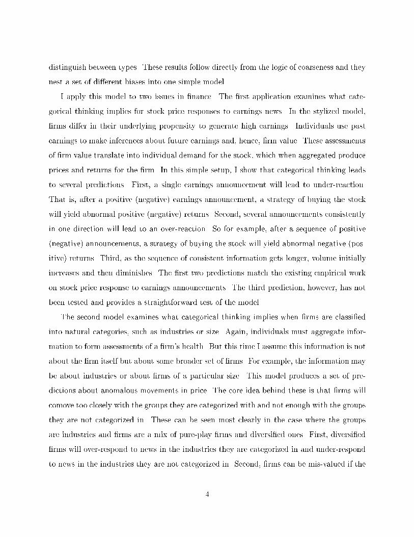
distinguish between types. These results follow directly from the logic of coarseness and they

nest a set of di�erent biases into one simple model.

I apply this model to two issues in �nance. The �rst application examines what cate-

gorical thinking implies for stock price responses to earnings news. In the stylized model,

�rms di�er in their underlying propensity to generate high earnings. Individuals use past

earnings to make inferences about future earnings and, hence, �rm value. These assessments

of �rm value translate into individual demand for the stock, which when aggregated produce

prices and returns for the �rm. In this simple setup, I show that categorical thinking leads

to several predictions. First, a single earnings announcement will lead to under-reaction.

That is, after a positive (negative) earnings announcement, a strategy of buying the stock

will yield abnormal positive (negative) returns. Second, several announcements consistently

in one direction will lead to an over-reaction. So for example, after a sequence of positive

(negative) announcements, a strategy of buying the stock will yield abnormal negative (pos-

itive) returns. Third, as the sequence of consistent information gets longer, volume initially

increases and then diminishes. The �rst two predictions match the existing empirical work

on stock price response to earnings announcements. The third prediction, however, has not

been tested and provides a straightforward test of the model.

The second model examines what categorical thinking implies when �rms are classi�ed

into natural categories, such as industries or size. Again, individuals must aggregate infor-

mation to form assessments of a �rm's health. But this time I assume this information is not

about the �rm itself but about some broader set of �rms. For example, the information may

be about industries or about �rms of a particular size. This model produces a set of pre-

dictions about anomalous movements in price. The core idea behind these is that �rms will

comove too closely with the groups they are categorized with and not enough with the groups

they are not categorized in. These can be seen most clearly in the case where the groups

are industries and �rms are a mix of pure-play �rms and diversi�ed ones. First, diversi�ed

�rms will over-respond to news in the industries they are categorized in and under-respond

to news in the industries they are not categorized in. Second, �rms can be mis-valued if the

4

industry they are classi�ed in has a price-to-earnings ratio that is very di�erent from the

industries they are in. When this e�ect is large, it can lead to so-called negative stubs, such

as the Palm and 3-Com example, in which a �rm appears to trade for lower value than the

stock it holds. The latter prediction, therefore, provides one interpretation of the empirical

work on negative stubs and tracking stocks. The �rst predicition, however, has not been

tested.

The rest of the paper is laid out as follows. Section 2 sketches a simple example which

highlights the important intuitions of the model. Section 3 lays out the general model of

categorical thinking. Section 4 presents the earnings reaction application to �nance. Section

5 presents the application to natural categories in �nance, such as industry. Section 6

concludes.

2 Simple Example

A simple example will illustrate how categorical thinking operates. Suppose a boss is in-

terested in evaluating an employee who engages in a project each period. The outcome of

the project is stochastic and is either good (1) or bad (0). The quality of the employee

determines the odds that each period's project turns out good or bad. The employee's type

t is either good G, okay O or bad B. A good employee produces a good outcome with

probability g > 12, a bad employee produces it with probability b = 1 � g < 1

2and an okay

employee produces it with probability 12. Let's assume that the boss has priors which are

symmetric but put more weight on the employee being okay, so p(O) > p(G) = P (B).

Each period the boss observes the project outcome and must forecast the next period's

outcome. Let d be the data observed so far. For example, d might equal 0011 indicating

the agent had 2 failures and then had 2 successes. Let e be the event being forecasted, for

example whether the next project will turn out good or bad. The task facing the boss is to

predict e given d. A Bayesian with knowledge of the mdoel would form beliefs as:

p(ejd) = p(ejG)p(Gjd) + p(ejO)p(Ojd) + p(ejd)p(Bjd)

5

It's easy to see that there will exist functions x(d) and y(d) so that:

p(1jd) = g � x(d) +1

2� (1� x(d)� y(d)) + (1� g) � (y(d))

Here x(d) is increasing in the number of 1s in the past and y(d) is increasing in the number

of 0s. This is quite intuitive. The Bayesian merely sees how many goods there have been

and updates his or her probabilities over all possible types. To make forecasts, he assesses

probability of a 1 for each type, multiplies by the updated probabilities and then adds them

all together. If the Bayesian model were to be taken literally, it would suggest that the boss

is keeping track of all possibilities and incorporating them all in making forecasts.

Consider the following alternative. Suppose instead of keeping track of all possibilities,

the boss imply makes his best guess as to whether the employee is good, bad or okay and

then uses this best guess to make predictions. For example, if the past performance history

is roughly balanced between 1 and 0s, the employer decides that the employee is an okay

one and forecasts probability 12of outcome 1 on the next project.

Experimental evidence in psychology supports this idea that individuals focus on one

category, at the exclusion of others. Murphy and Ross (1994) present a simple experiment

which illustrate this point. Subjects viewed large sets of drawings from several categories

(\those drawn by Ed", \those drawn by John"...), where each category had its own features.

The participants were then asked to consider a new stimulus (e.g. a triangle) and asked which

category it �t best. They were then asked the probability it would have a speci�ed property,

such as a particular color. They found that participants' assessment of this probability

depended on the frequency with which this property appeared in the chosen category. But

it did not depend on it's frequency in alternative categories. Other evidence is provided in

Malt, Ross and Murphy (1995). In one experiment, subjects were given the following story:

Andrea Halpert was visiting her good friend, Barbara Babs, whom she had

not seen in several years. The house was lovely, nestled in a wooded area outside

of the small Pennsylvanian town. Barbara greeted her at the door and shoed her

into the spacious living room. They talked for a while and then Barbara went to

6

make some tea. As Andrea was looking around, she saw a black-furred animal

run behind a chair. [She hadn't realized that Barbara had a dog as a pet]/[She

hadn't realized that Barbara had a pet, but thought it was probably a dog.] Barbara

came back and they caught up on old times. Did Barbara know what happened

to Frank? Had Andrea been back to some of their old haunts?

In the high-certainty condition, subjects are given the �rst sentence in italics, whereas in the

low-certainty condition they are given the second sentence in italics. Following this story,

subject were given a set of questions, one of which was \What is the probability that the

black-furred animal chews slippers?". They �nd that individuals report the same probability

irrespective of the condition. An independent test showed that subjects in fact believed the

manipulation: they assessed the probability that the animal was dog as lower in the low-

certainty condition. But this did not in uence their prediction: they predicted as if the

animal were basically a dog.

A �nal experiment is provided by Krueger and Clement (1994). They ask subjects to

guess the average high and low temperatures between 1981 and 1990 in Providence, Rhode

Island. Each subject was given a sequence of randomly generated month and day pair, e.g.

July 20, and asked to guess a temperature. They �nd that subjects are fairly accurate at

their guesses on average. The average forecast error across all months is zero, suggesting no

particular bias towards guessing too warm or too cold. But they �nd the following interesting

pattern. A noticeable jump in temperature occurred when the month changed. That is, for

two equally spaced days, the di�erence in predicted temperature was greater when the days

straddled a month than when they were in the same one. One intuitive interpretation is that

subjects used the month as the category, focusing on that to make their predictions. During

warming periods (e.g. Spring), they under-forecasted the temperatures of days later in the

month and over-forecasted temperatures of early days. Instead of viewing April 29 as partly

an April day and mostly a May day, they erred by forecasting a temperature for it that was

too close to the April mean. As the authors note:

Willard Scott, the noted weatherman of NBC's \Today" program exclaimed on

7

January 27, 1994, \Geez, come on, February".

These experiments make it clear that a good operating assumption for now will be that

individuals use the most likely category.

Returning to the example, let c�(d) be the chosen category G, O or B.5 This choice will

be governed by the posteriors: the most likely category will be chosen. In other words, if

the Bayesian were forced to choose one category, he would choose c�(d). Formally:

c�(d) =

8>>>>><>>>>>:

G if x(d) = maxfx(d); y(d); 1� x(d)� y(d)g

O if 1� x(d)� y(d) = maxfx(d); y(d); 1� x(d)� y(d)g

B if y(d) = maxfx(d); y(d); 1� x(d)� y(d)g

(1)

Note that this formalism presumes correct choice of category, with people using the true

probability distribution over categories. For example, they do not mistakenly ignore base

rates in choosing the categories.6

Intuitively, when there are a lot of good outcomes, G will be chosen, when there are a lot

of bad outcomes B will be chosen and when good and bad outcomes are roughly balanced,

O will be chosen. Predictions are now extremely simple. Let k(ejd) be the prediction of a

categorical thinker:

k(ejd) =

8>>>>><>>>>>:

g if c�(d) = G

12

if c�(d) = O

b if c�(e)c�(d) = B

What kind of bias does this simple decision rule generate? First, let us focus on the

case where c�(d) = O. This means that the data is roughly balanced with around the same

number of good and bad projects. The categorical forecast here will be 12of a good outcome.

Di�erencing this from the Bayesian suggests that the bias is:

k(ejd)� p(ejd) = (1

2� g)x(d) + (

1

2� b)y(d)

5In this simple example, categories and types will be equivalent.6Base rate ignorance would amount to ignoring the base line probability of a category p(c) in choosing

categories. Kruschke (1996) surveys the evidence on whether base rates are in fact used in choosing categoriesand argue that the evidence is remarkably mixed.

8

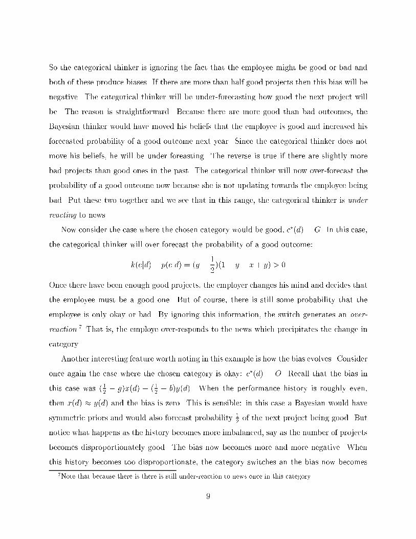
So the categorical thinker is ignoring the fact that the employee might be good or bad and

both of these produce biases. If there are more than half good projects then this bias will be

negative. The categorical thinker will be under-forecasting how good the next project will

be. The reason is straightforward. Because there are more good than bad outcomes, the

Bayesian thinker would have moved his beliefs that the employee is good and increased his

forecasted probability of a good outcome next year. Since the categorical thinker does not

move his beliefs, he will be under-foreasting. The reverse is true if there are slightly more

bad projects than good ones in the past. The categorical thinker will now over-forecast the

probability of a good outcome now because she is not updating towards the employee being

bad. Put these two together and we see that in this range, the categorical thinker is under

reacting to news.

Now consider the case where the chosen category would be good, c�(d) = G. In this case,

the categorical thinker will over-forecast the probability of a good outcome:

k(ejd)� p(ejd) = (g �1

2)(1 + y � x + y) > 0

Once there have been enough good projects, the employer changes his mind and decides that

the employee must be a good one. But of course, there is still some probability that the

employee is only okay or bad. By ignoring this information, the switch generates an over-

reaction.7 That is, the employe over-responds to the news which precipitates the change in

category.

Another interesting feature worth noting in this example is how the bias evolves. Consider

once again the case where the chosen category is okay: c�(d) = O. Recall that the bias in

this case was (12� g)x(d) + (1

2� b)y(d). When the performance history is roughly even,

then x(d) � y(d) and the bias is zero. This is sensible: in this case a Bayesian would have

symmetric priors and would also forecast probability 12of the next project being good. But

notice what happens as the history becomes more imbalanced, say as the number of projects

becomes disproportionately good. The bias now becomes more and more negative. When

this history becomes too disproportionate, the category switches an the bias now becomes

7Note that because there is there is still under-reaction to news once in this category.

9

positive. In otherwords, the move from under-reaction to over-reaction is not monotonic.

The under-reaction becomes more and more severe until it translates into over-reaction at

the point of category switch.

This example illustrates several features of categorical thinking. First, the tendency to

change opinions infrequently can lead to under-reaction. Second, this bias can increase as

the weight of information that has been under-responded to increases. Finally, when beliefs

are changed they will lead to an over-reaction.

3 General Model

How do we go about generalizing this example? In this simple example, categorization

involves choosing one of the possible types and presuming that it the correct one. This

choice can be put in broader terms. The set of beliefs the Bayesian can have after seeing

some data forms a simplex: (p(G); p(O); P (B)). And he updates by choosing a belief in this

simplex. The categorical thinker, however, can only hold one of three beliefs in that simplex:

(1,0,0), (0,1,0) and (0,0,1). This motivates how this example is generalized into a model of

coarseness: a categorical thinker is forced to choose from a limited set of beliefs rather than

from the full, continuous space available to the Bayesian.

3.1 Setup

I am going to model categorization in an abstract inference set-up, one which admits many

di�erent applications. In this setup, an individual is attempting to forecast the outcome of

a statistical process on the basis of limited data. De�ne D to be the set of data that the

individual may observe prior to making forecasts and E to be the set of events or outcomes

that the individual will be making forecasts about.8 Let T be the set of underlying types.

Each type determines the process which generates the outcomes. De�ne p(ojd; t) to be the

8Of course, these sets will not necessarily be exclusive. In the example above, data was information aboutproject success, while events to be forecasted were also information about project success.

10

true conditional probability distribution which generates the data if the true type were t.

I will assume that the prior probability of any one type is de�ned by p(t) and that p(djt)

de�ne the conditional probability of observing some data.

The bench-mark for inference will be the Bayesian who has full knowledge of the structure

of the underlying stochastic process. This Bayesian would make the forecast:

p(ojd) =Zt2T

p(ojd; t)p(tjd) (2)

As noted earlier, cognitively, this would amount to updating the probability of every state

given the data d, the probability of e for each type and then summing over all types.

De�ne Q to be the full set of distributions over types. Each q 2 Q de�nes a probability

for each type. In equation 2 the Bayesian chooses one distribution from this set Q and

makes forecasts using this distribution. In other words, nothing constrains the Bayesian

from choosing the distribution of his choice and he therefore chooses the optimal posterior.

3.2 Categories

Coarseness of categories will be modelled as a constraining what distribution can be chosen

from the full set Q. So a category in this context will correspond to a speci�c distribution

over types. Let C be the set of categories and c de�ne a speci�c category. Each category

has associated with it a particular point in the posterior space. This point represents the

category, call it qc(t). In the simple example before, we were presuming that C contained

three elements whose associated distributions were (1; 0; 0); (0; 1; 0); (0; 0; 1). The second

feature of categories is that they must partition the posterior space. In other words, while

the Bayesian chooses any given point, the categorical thinker will end up choosing one of the

categories. The map which dictates what category gets chosen for each possible posterior in

Q. In the example above, the partition was implicitly given by equation 1. For example, the

posterior (.1,.8,.1) may be assigned to the O category. Let c(q) be the function which assigns

each point in the posterior space to a category. I will assume this function is continuous

in the sense that the implied partition is continuous. It will also be useful to de�ne p(c)

11

to be the probabilityRt p(t)qc(t), in other words the base-rate of a category will be the

probability of the underlying distribution. Similarly, de�ne q(ojd) =Rt q(t)p(ojd) to be

the conditional probability distribution over outcomes for any given q and p(djc) to be the

analagous distribution over data. So the set of categories is de�ned by two things: c(q)

which maps every posterior to a category and qc(t) which dictates what speci�c posterior

the category is represented by.

But we do not want to allow for any arbitrary partition. Speci�cally, as in the example,

the category which best �ts the data should be chosen. De�ne c�(d) to be the category

associated with the posterior that data d leads to. Speci�cally, c�(d) � c(p(tjd)). Every

categorization must satisfy the condition that the category associated with some data is the

one that is most likely to generate that data:

c�(d) 2 argmaxcp(djc)p(c) (3)

So the chosen category must be amongst the ones that the Bayesian would choose if forced

to choose one category.9 As before, the base-rate of each category is taken into account

in choosing that category. And as before the choice of category is optimal: it is what the

Bayesian would choose if forced to choose one category.

Having chosen a category, the categorical thinker uses it to make predictions. Speci�cally

if we de�ne k(ojd) to be the forecasts of a categorical thinker then:

k(ojd) � qc�(d)(ojd) =Ztp(ojt; d)qc�(d)(t) (4)

In other words, he uses the probability distribution associated with the category to make

predictions.10

9This equation may not be binding in many cases as we will see below.10This de�nition makes clear that while categories de�ne a partition of the posterior set, they are more.

Di�erent categorizations that produce identical partitions will not necessarily result in the same predictions.In the example above, the categories were (1; 0; 0); (0; 1; 0) and (0; 0; 1) or the vertices of the simplex. Supposethey had been (1��1; 0; 0); (0; 1��2; 0); (0; 0; 1��3), points close to the vertices but not the vertices themselves.For some �i this will produce an identical partition of the simplex. But the forecasts as de�ned above usingthese categories will not be the same since the distribution used to make predictions will be di�erent. Soeven though the choice of category will look the same, what is done once the category is chosen will bedi�erent.

12

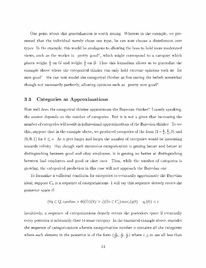
One point about this generalization is worth noting. Whereas in the example, we pre-

sumed that the individual merely chose one type, he can now choose a distribution over

types. In the example, this would be analagous to allowing the boss to hold more moderated

views, such as the worker is \pretty good", which might correspond to a category which

places weight 12on G and weight 1

2on B. Thus this formalism allows us to generalize the

example above where the categorical thinker can only hold extreme opinions such as \for

sure good". We can now model the categorical thinker as �ne-tuning the beliefs somewhat

though not necessarily perfectly, allowing opinions such as \pretty sure good".

3.3 Categories as Approximations

How well does the categorical thinker approximate the Bayesian thinker? Loosely speaking,

the answer depends on the number of categories. But it is not a given that increasing the

number of categories will result in in�ntesimal approximations of the Bayesian thinker. To see

this, suppose that in the example above, we produced categories of the form (1� kn; kn; 0) and

(0; 0; 1) for k � n. As n gets larger and larger the number of categories would be increasing

towards in�nity. But though each successive categorization is getting better and better at

distinguishing between good and okay employees, it is getting no better at distinguishing

between bad employees and good or okay ones. Thus, while the number of categories is

growing, the categorical prediction in this case will not approach the Bayesian one.

To formalize a su�cient condition for categories to eventually approximate the Bayesian

ideal, suppose Cn is a sequence of categorizations. I will say this sequence densely covers the

posterior space if:

(8q 2 Q; epsilon > 0)(9i)(8j � i)(9c 2 Cj)maxt(q(t)� qc(t)) < �

Intuitively, a sequence of categorizations densely covers the posteriors space if eventually

every posterior is arbitrarily close to some category. In the canonical example above, consider

the sequence of categorizations wherein categorization number n contains all the categories

where each element in the posterior is of the form ( 12m; 12j; 12i) where i; j;m are all less than

13

or equal to n. Thus, categorization number 0 would be the one used in the example: the

vertices of the simplex. Categorization number 1 would have the vertices but would also

include categories of the form (12; 12; 0) and permutations of these and so on. As n increases,

these categories would eventually come to cover the simplex. This de�nition readily produces

the following result.

Proposition 1 Let Cn be a sequence of categorizations that densely covers the posterior

space. If kn(ojd) is the prediction associated with categorization Cn, then:

(8o; � > 0)(9i)(8j � i)[kn(ojd)� p(ojd)] < �

In other words, the categorical thinker gets arbitrarily close to the Bayesian.

Proof: The proof is straightforward. By de�nition, one can always choose an n

large enough so that the qc�n(d) is arbitrarily close to p(tjd), the correct posterior.

This in turn means that the predicted probabilities will be arbitrarily close.

3.4 Biases in Categorical Thinking

This proposition shows that when categories are �ne enough, the categorical thinker will

approximate the Bayesian one. But what happens when categories are coarse? Three kinds

of bias arise. First as was seen in the coin example, because categorical thinkers change their

beliefs rarely, they are often under-reacting to information. Second, also seen in the coin

example, when changes in categories do occur, they are discrete resulting in an over-reaction.

Finally, and this was not present in the coin example, categories collapse types: this can

lead to biases even when there is no updating of types, simply because the same prediction

function is used for several distinct types.

Formally, let d be some data and n be some news. We are interested in how beliefs

are revised in the face of news, so in how k(ojd) is revised into k(ojd&n). Comparing this

revision to the Bayesian benchmark of p(ojd)-p(ojd&n) tells whether the categorical thinker

responded appropriately or not and a way of quantifying bias. In this context, it will be

14

useful to de�ne news as being informative about outcome o whenever p(ojd)�p(ojd&n) 6= 0,

in other words when the news should cause a change in beliefs.

3.4.1 Under-Reaction

Consider the case where the news n does not lead to a change in category. When there is no

change in category:

k(ojd)� k(ojd&n) = qc�(d)(ojd)� qc�(d)(ojd&n)

But the two terms in the right hand side need not equal each other. Therefore, unlike in

the example, in this more general setup predicted probabilities can change even though the

category does not change. This in turn may make it so that even when there is no change

in category, there may not be under-reaction.

A simple example illustrates. Suppose we are forecasting ips of a coin and there are two

processes governing the coin. One process is positively auto-correlated and has equal chances

of generating heads and tails on the �rst ip. The other process generates much more tails

than heads on the �rst ip but is slightly mean-reverting in that the bias towards tails is

lowered in the second ip (though there is still a bias towards heads). Suppose that the auto-

correlated one is thought to be slightly more likely ex ante. In the absence of any data, the

categorical thinker would predict probability 12. After seeing a tail, what does she do? If she

has not switched category, the time when we expect under-reaction she'll actually predict

a higher chance of tails because of the positive auto-correlation. The Bayesian, however,

because she considers the other category will still update towards tails on the second ip,

but less so because the alternative category is being considered and in this alternative, the

bias towards tails decreases.

Certain assumptions, however, guarantee that there will be under-reaction to news that

does not change categories. De�ne the types to be a su�cient statistic if:

(8o; t; d)p(ojd; t) = p(ojt)

15

In other words, if the type completely summarizes the data then types are a su�cient

statistic. Also, de�ne the size of news n for outcome o given data d to be jp(ojd&n)�p(ojd)j.

These de�nitions readily provides the following result:

Proposition 2 Suppose types are a su�cient statistic and that a particular news is infor-

mative about an outcome o given data d. Categorical thinkers will under-respond to this news

if it does not lead to a category change. Formally, if c�(d) = c�(d&n), then

jk(ojd)� k(ojd&n)j < jp(ojd)� p(ojd&n)j

Moreover, as the size of the news increases, the extent of under-reaction increases.

Proof: Note that jp(ojd)� p(ojd&n)j is positive because the news is assumed to

be informative. But

jk(ojd)� k(ojd&n)j =

= qc�(d)(ojd)� qc�(d)(ojd&n)

= qc�(d)(o)� qc�(d)(o) = 0

because types are a su�cient statistic.

The size e�ect follows mechanically now because jp(ojd)�p(ojd&n)j is increasing

while k(ojd)� k(ojd&n) = 0.

The intuition behind this proof is quite simple. Because types are a su�cient statistic,

predicted probabilities only change when types or categories change. Therefore, predicted

probabilities do not change in response to news that does not change categories. But because

the news is informative, we know they should and the lack of a change generates under-

reaction.

3.5 Over-Reaction

What happens when categories change? In the above example, we saw that category change

leads to a clear-cut over-reaction. As with under-reaction, to recover the result in this general

16

context, we will have to assume that types are su�cient statistic. To formalize this notion,

we will need a few de�nitions �rst. For two categories c1 and c2 and data d, an outcome is

distinguishable qc1(ojd) 6= qc2(ojd). In other words, an outcome is distinguishable if the two

categories lead to di�erent predictions on it.

Proposition 3 Suppose data d has been observed and then news n is observed and types are a

su�cient statistic. If (1) news n leads to a change in categories and (2) o is distinguishable

for categories c�(d) and c�(d&n), then if the size of the news n is su�ciently small, the

categorical thinker will over-react to it. Speci�cally:

jk(ojd)� k(ojd&n)j < jp(ojd)� p(ojd&n)j

Proof: We know the left hand side is strictly positive because the news is dis-

tinguishable and types are a su�cient statistic. As the news gets small, however,

the right hand side tends towards zero.

The intuition behind this result is extremely simple. Since changes in categories are discrete,

small amounts of information can trigger it. Thus, even though Bayesian decision making

would dictate only a small change in predicted probabilities, the categorical thinker will show

a large, discrete change in expectations, thus precipitating an over-reaction.

3.6 Misinterpretation

A �nal source of bias in this model comes purely from the fact that data can be misinterpreted

because a coarse category, rather than the correct type is used. To make this type of problem,

let us focus on situations where there is full information about the underlying type. De�ne

data d to generate a unique type if there exists some type t such that p(tjd) = 1. In many

contexts, prediction is not about inferring type but instead about translating past data into

future predictions. In the example from Section 5, investors have data on what �rm an

industry is in (this is the type) and must use the type to translate information about how

industries are doing into a prediction for the speci�c �rm at hand. But because categorical

17

thinkers may not have categories for each particular type, they may end up mistaking this

translation.

Suppose data d generates a unique type t and the individual faces some news n. The

Bayesian would forecast p(ojt; n). The categorical thinker on the other hand forecasts:

k(ojd; n) = qc�(d;n)(ojn)

= qc�(d;n)(t)p(ojt; n) +Zs6=t

p(ojn; s)qc�(d;n)(s)

This will equal the Bayesian forecast p(ojt; n) if qc�(d;n)(t) = 1. In other words, if the category

chosen for d; n is in fact the type distinguished by the data itself. If not, there is room for

misinterpretation. In other words, whenever the categories lump together the posterior which

places full weight on type t with other distinct posteriors, then news will be construed to

mean something other than it is.

3.7 Representativeness

This section makes clear that the simple assumption of coarseness leads to straightforward

results and generates some systematic biases. As highlighted in Mullainathan (1999), a

second feature of categorization when combined with coarseness yields yet more predictions.

In fact, together these two features produce behavior that are quite close the psychology

evidence on decision making.

Labeled representativeness, the second feature of categorical thinking is that a category

is not just de�ned by a point in the posterior space. Instead each category has associated

with it a representativeness function. I make two assumptions about this function. First, I

assume that representativeness is proportional to the true probability distribution for that

category. Events that are more likely, in a probability sense, are also more representative.

Second, I assume that an outcome is more representative when that outcome is more likely

to generate that category. For example suppose outcome e1 and e2 have the same probability

under category c. If c�(e1) = c, but c�(e2) 6= c, then e1 is considered more representative.

18

More generally, I will assume that outcomes which are further from being in the category

are considered to be less representative.

As before, people choose the category optimally. They merely use the representativeness

function instead of the probability function to predict outcomes. To make predictions by

asking how representative a particular outcome would be of the chosen category.

The e�ect of representativeness is easily understood by returning to our stylized example.

Categorization is as before: a large fraction of good outcomes will lead the supervisor to

decide the employee is good, a large fraction bad will lead the supervisor to decide he

is bad, and a roughly balanced one will lead the supervisor to decide is okay. But the

representativeness function is more complicated than the probability function used before.

For example, in the absence of representativeness, classifying the employee as Ok would lead

the boss to predict probability 12of success in the future. But this need not be the case now.

To take a speci�c case, suppose that 2 good outcomes in a row would lead to classi�cation

of good whereas a 3rd good outcome would cause the boss to change his mind and call the

employee good.

Suppose the boss has seen 2 successful projects; she individual will choose the okay

category. Since three successful proects would not elicit a categorization of ok, it is by

de�nition less representative. Hence after 2 successful projects, the employer would show

a bias towards predict a bad project. This generates a second reason for under-reaction.

Not only is the employer not incorporating the news in 2 heads and updating, he is now

predicting that a tail will happen simply to make the sequence more representative of the

okay category. This result matches experimental �ndings on the Law of Small Numbers

or the Gambler's fallacy. People often demonstrate such a predilection for expecting mean

reversion, for expecting sequences to \right" themselves out (2 heads in a row should be

\corrected" by a tail).

But consider what will be predicted after three good outcomes are observed. Now the

boss will classify the empoyee as good. But since three goods followed by a succcess may

not be a part of the good category, the boss is now biased towards over-forecasting good.

19

Again, the over-reaction when crossing the category boundary is exaggerated. Instead of

simply forecasting the mean probability of good outcomes for the good category, the boss is

even further exaggerating the probability of a good outcome simply because a bad outcome

would make the sequence more representative of a di�erent category. This result matches

the experimental �ndings on the Hot Hand. People perceive this coin as \hot" and over-

estimate the odds that it will continue. Notice the contrast with the Law of Small Numbers.

Whereas it predicts the bias towards expecting runs to end, the Hot Hand emphasizes the

bias towards expecting runs to continue. Despite their apparent contradictions, both arise

intuitively and in a structured way in the same model.

In fact, they appear with enough structure that we can make predictions about when one

will dominate, as can be seen in this example. After a single good, the bias towards a bad

project will be weak. As the run length builds up, the bias towards a bad outcome (towards

expecting the run to end) increases. When the run length got long enough, however, the

bias became towards expecting another good project (or the run to continue). This speci�c

pattern in which we expect the two forces to operate provides an easy to test, out of sample

prediction of the model.

Another interesting feature of adding representativeness is that forecated probabilities

need not be monotonic: an outcome which is a strict subset of another may be seen as

more probable. In the above example, after two good outcomes, when the employee is still

thought of as only okay, 1110 (or one more good but followed by a bad outcome) may be

seen as more likely than 111 (just one more good). This is because, under some parameter

values, 1110 would elicit the okay category and hence be more representative than 111 which

may not. This non-monotonocity in turn matches experimental evidence on the conjunction

event. People sometimes report the event \A and B" as being more likely than the event

\A" by itself. Again, we will see the model's speci�city allows extremely precise predictions

about when the conjunction e�ect should arise.

In short, the addition of representativeness allows the model to mimic a variety of exper-

imental data on decision-making. This paper focuses on the coarseness case alone because

20

it provides a much more tractable model for economic applications, which I turn to now.

4 Investor Response to Earnings Announcements

In this section, I sketch an extremely simple model of how categorical thinkers might respond

to earnings announcements. Undoubtedly, as with any model, the speci�c predictions will

depend on the exact earnings process that is assumed. For simplicity, I will simply expand

on the example in Section 2, just to illustrate the kinds of predictions that such a model

might make.11 Consider a single �rm who has earnings each period, Et which are paid out

as dividends. These earnings can either be +1 or 0 and are iid distributed. The �rm has

an underlying probability p of generating good earnings (+1). I will assume that there are

three types of �rms: good, okay and bad, where good �rms have probability g of generating

good earnings, bad �rms have probability b = 1 � g and okay forms have probability 12.

As before, the prior probability on the three types is symmetric with the okay type having

greater probability than the other two. To guarantee continuous learning, however, I will

assume that each period the �rm has an iid probability s of changing types. If it changes, it

gets a fresh draw from the prior distribution.

There is a continuum of individuals indexed between 0 and 1, each of whom is a cate-

gorical thinker. To model heterogeneity, I will assume that each of these individuals holds a

slightly di�erent categorization. Individual 0 holds the categorization similar to the example

in Section 2: the vertices (1; 0; 0); (0; 1; 0); (0; 0; 1). Individual j, however holds the catego-

rization (1� (1� j)�; j�; 0), (0; 1; 0) and (0; j�; 1� (1� j)�). In other words, for the category

G and B, instead of using the vertices, he uses a point slightly more interior to the simplex.

What this means is that as j decreases, the individual needs fewer successes to switch from

the okay category to the good category or fewer failures to switch from the okay to the bad

11Note, however, that the predictions will depend on the speci�c context. If earnings processes are auto-correlated, then the predictions here might well change. Categorical models only provide a framework withwhich to make predictions. The exact predictions, as with Bayesian models, will depend on what is assumedabout the environment. In fact, one of the useful feature of the categorical thining framework is it's abilityto make predictions in any context once the categories are speci�ed.

21

category.

Let qjt be the perceived probability by individual j at time t that the �rm will generate

good earnings. Speci�cally if ht is the history of earnings qjt = kj(1jht) where kj(�) is

the categorical forecast of individual of individual j. Let r be the interest rate applied to

discounting future earnings. What will be the person's perceived value of the �rm? This

period he received earnings Et. Next period, he expects qjts (because the �rm may have

changed type and qjts2 for the period after. When discounted this looks like:

Et + qjt

�s

1 + r

�+�

s

1 + r

�2+ � � �

!= Et + qjtA

where I've de�ned A to be the constant associated with that sum. De�ne Vjt to be the

perceived valuation at time t by individual j. Let Vt be the actual value of the �rm in the

market. Suppose demand curves are linear with constant � so that each individual demands

are proportional to demand ��(Vjt�Vt). Market clearing implies that Vt =RVjt = Et+

RqjtA.

In other words, the market clearing value of the �rm is merely the current period earnings

plus the average belief about the �rm's underlying propensity to generate good earnings.

To understand misreactions, it will be useful to de�ne portfolio returns. Let R(ht) be

the net present value of the dividend return to buying a the stock at time t if history ht

has occurred minus the purchase price. So R() positive indicates that there are positive

abnormal returns, whereas R() negative indicates that there are negative abnormal returns.

With this in place, the results from Section 3 readily translate into a serious predictions

about how �rms earnings will respond as codi�ed in the following proposition.

Proposition 4 Suppose that the earnings history ht is roughly balanced. Then there will

exist n� such that:

1. A sequence of n < n� positive earnings announcements results in R(ht11 � � �1) yielding

a postive return. A sequence of n < n� negative earnings announcements results in

R(ht00 � � �0) yielding a negative return. In other words, the market under-responds to

less than n good or bad earnings announcements.

22

2. A sequence of n > n� positive earnings announcements results in R(ht11 � � �1) yielding

a negative return. A sequence of n > n� negative earnings announcements results in

R(ht00 � � �0) yielding a posiive return. In other words, the market over-responds to

more than n good or bad earnings announcements.

This result follows directly from the propositions in Section 3 and 2. A few consistent

earnings announcements will lead to under-response because there is no change in category,

whereas several good ones will lead to a change in category and over-response. One inter-

esting feature to note, however, is that the heterogeneity means that the under-response

may not be non-linear in aggregate. In Section 2, we saw that the individual under-response

builds up, becoming an increasing under-response before becoming an over-response. In the

aggregate, however, because some people switch categories earlier, the net mis-response need

not be non-monotonic. But what this means is that agents will be trading with each other.12

Since the market price switches to over-response when exactly half the agents have switched

categories, this also means that the mis-response is also highest when half have switched.

This is formalized in the following proposition.

Proposition 5 Suppose that the earnings history ht is roughly balanced. Let n� be the n�

from the previous proposition. Then for a streak of good or bad earnings announcements,

volume is increasing in n until n > n� at which point it diminishes.

In other words, heterogeneity endogenously builds up as some agents have switched categories

before others. Speci�cally, agents with lower j will switch earlier and as the streak continues,

eventually all the agents will switch and the heterogeneity will disappear as will trading

volume.

While this is a highly stylized example, it does illustrate exactly how the propositions in

Section 3 on under- and over-reaction can translate directly into a �nancial market. It also

illustrates how the sharp changes induced by categorical changes need not show up only in

prices but can translate into dramatic trading volume.

12I will presume that each period agents start o� with a new endowment of stocks so that there is historydependent in trading.

23

5 Application 2: Natural Firm Categories

In a second example, we will consider �rms that are in natural categories. For example,

some �rms are thought of as large, some are though of as small. Perhaps the most natural

category. Consider �rms that are in one of two industries, with fraction t of their earnings in

industry 0 and fraction 1� t in industry 1. This t denotes the type of the �rm and suppose

it is publicly observable for each �rm. In this sense, we will be considering the case of Section

3.6. Suppose each period, the �rm pays a dividend Es which is either +1 or 0 and does so

with probability ps. This probability ps depends on the probabilities of the industry the �rm

is in. Let as be the probability for �rms in industry 0 doing well at time s and bs be the

probability for �rms in industry 1 doing well at time s. Assume that:

ps = tas + (1� t)bs

At the end of period s, the probabilities for both industries in the next period are shown,

so as+1 and bs+1 are made public. These are drawn from a uniform distribution. With this

information and when given information on the type of the �rm, the Bayesian at time s

would value the �rm at:

Es +r

2(1 + r)+tas+1 + (1� t)bs+1

1 + r

In other words, the value of the �rm is the value of the current earnings plus the guess of

earnings next period (which depends on type plus the discounted value of all other future

earnings (which are type independent).

Now consider a categorical thinker who has categories (1; 0) and (0; 1) so that he can

only think of �rms which are fully in one industry. Suppose further that the partition is such

that �rms which are below some threshold t < J are classi�ed to be in industry 0 and those

above the threshold are classi�ed to be industry 1. Then the categorical thinker would value

the diversi�ed �rm at:

Es +r

2(1 + r)+

as+1

1 + rif t < J

Es +r

2(1 + r)+

bs+1

1 + rif t � J

24

Thus for �rms with 0 < t < J will over-respond to news about industry 0 and under-respond

to news about industry 1. Similarly for �rms with J � t < 1 he will over-respond to news

about industry 1 and under-respond to news about industry 0.

In other words, for diversi�ed �rms, the industries they are classi�ed in will make a

di�erence. They will over-respond to news about industries they are put in and under-

respond to news about industries they are not classi�ed in. More generally, they will comove

too much with the industry they are thought to be in and too little with the other one.

This logic also can generate �ndings about stubs. Consider a �rm which is :75 in industry

0 which is having terrible times and :25 in industry 1 which is doing extremely well. If it

is classi�ed as being in industry 0, it will have a much lower valuation. In fact if industry

0 is doing poorly enough, the �rm will look like it has negative valuation of it's holdings

in industry 0 because the entire �rms future earnings streams, including those in the good

industry are being valued using the outlook of industry 0.

Thus this simple categorization model makes straightforward and novel predictions about

where misvaluations ought to occur when thinking about diversi�ed �rms. Relabeling these

industry categories to be other natural categories such as glamor and value or large and small

will suggest a set of predictions about comovement of �rms with their natural categories as

well as when over and under-valuation will occur.

6 Conclusion

To summarize, the coarseness induced by categories provides an extremely simple framework

for thinking about a wide variety of biases. As the �nancial applications make clear, the

model is ultra-simple to apply and readily makes testable predictions.

25