three-channel correlation analysis: a new technique to ...seismain/pdf/bssa06-inst.pdf ·...

258

Bulletin of the Seismological Society of America, Vol. 96, No. 1, pp. 258–271, February 2006, doi: 10.1785/0120050032

Three-Channel Correlation Analysis: A New Technique to Measure

Instrumental Noise of Digitizers and Seismic Sensors

by Reinoud Sleeman, Arie van Wettum, and Jeannot Trampert

Abstract This article describes a new method to estimate (1) the self-noise as afunction of frequency of three-channel, linear systems and (2) the relative transferfunctions between the channels, based on correlation analysis of recordings from acommon, coherent input signal. We give expressions for a three-channel model interms of power spectral densities. The method is robust, compared with the conven-tional two-channel approach, as both the self-noise and the relative transfer functionsare extracted from the measurements only and do not require a priori informationabout the transfer function of each channel. We use this technique to measure andmodel the self-noise of digitizers and to identify the frequency range in which thedigitizer can be used without precaution. As a consequence the method also revealsunder which conditions the interpretation of data may be biased by the recordingsystem. We apply the technique to a Quanterra Q4120 datalogger and to a Networkof Autonomously Recording Seismographs (NARS) datalogger. At a sampling rateof 20 samples/sec, the noise of the Q4120 digitizer is modeled by superposition ofa flat, 23.6-bit spectrum and a 24.7-bit spectrum with 1/f 1.55 noise. For the NARSdatalogger the noise level is modeled by superposition of a 20.8-bit flat spectrumand a 23.0-bit spectrum with 1/f 1.0 noise. The measured gain ratios between the digi-tizers in the Q4120 datalogger, smoothed over a tenth of a decade between 0.01 Hzand 8 Hz for data sampled with 20 samples/sec, are within 1.6% (or 0.14 dB) of thevalues given by the manufacturer. Finally, we show an example of seismic backgroundnoise observations at station HGN as recorded by both an STS-1 and a STS-2 sensor.Between 0.01 and 0.001 Hz the vertical STS-2 noise levels are 10–15 dB above theSTS-1 observations. The Quanterra Q4120 digitizer noise model enables us to excludethe contribution of the digitizer noise to be responsible for this difference.

Introduction

Broadband (BB) and very broadband (VBB) seismic sen-sors are used in global, regional, and even local seismolog-ical studies because of their wide-frequency response,low-self-noise level, and large dynamic range. Typical band-widths (all instrumental specifications in this introductionare taken from the manufacturers) for VBB sensors are fromaround 360 sec to 5 Hz (KS54000) or to 10 Hz (STS-1,CMG-1T). For BB sensors the bandwidths range between120 sec and 50 Hz (STS-2, KS-2000, CMG-3T) and 40 secand 50 Hz (Trillium). These bandwidths specify the fre-quency ranges in which the instruments have a (more or less)flat response to ground velocity. The self-noise of these sen-sors is typically close to the U.S. Geological Survey (USGS)New Low Noise Model (NLNM) (Peterson, 1993) over largefrequency bands (CMG-1T, about 300 sec to 20 Hz; STS-1,105 sec to about 2.5 Hz) or smaller bands (EP-300, 20 secto 5 Hz; CMG-40T, 10 sec to 1 Hz). In some frequencybands the output of the sensors can thus reflect, at most sites,

the Earth noise in the absence of seismicity, and the seismicrecords will not be influenced by the instrumental self-noise.At longer periods (above 200 sec) the NLNM is essentiallycoincident with the self-noise of the STS-1 (Wielandt,2002a), whereas current other broadband sensors show in-strumental noise above the NLNM (Widmer-Schnidrig,2003). To capture the large dynamic range of seismic signalsfrom ambient Earth noise to earthquakes as large as mag-nitude Mw 9.5 at 90� epicentral distance (Incorporated Re-search Institutions for Seismology [IRIS], 2003) the sensorsare designed to provide a large dynamic range (Wielandt andSteim, 1986). Broadband seismometers usually are of a forcebalance feedback design and have dynamic ranges up toroughly 160 dB.

Current high-resolution data-acquisition systems arespecifically designed to cover a large part of the bandwidthand dynamic range of the sensors. These digitizers are basedon delta-sigma modulators (e.g., Candy and Temes, 1992),

Three-Channel Correlation Analysis: A New Technique to Measure Instrumental Noise of Digitizers and Seismic Sensors 259

which decrease the quantization errors at lower frequenciesat the price of increased quantization errors at high frequen-cies. By using a high initial sampling rate (in the order oftens of kilohertz) the quantization error will decrease in thefrequency range of seismic interest (e.g., f � 200 Hz).Through the use of these “noise-shaping” digitizers the dy-namic range of seismic dataloggers, often expressed by asingle number representing the ratio of the largest to thesmallest signal that can be recorded (Bennett, 1948), mayrange up to about 145 dB. The representation of the behaviorof a digitizer by a single number is convenient but does notreflect the true dynamic behavior of the digitizer as functionof the frequency. First, the dynamic range of the digitizeris not a static value but depends on the sampling rate andthe frequency. The noise-shaping effect of the oversampleddelta-sigma digitizers results in a larger dynamic range atlower sample frequencies. Second, at lower frequencies(e.g., f � 1 Hz) the self-noise of the digitizers will increaselike in any other active electronic component. This so-called1/f type noise may therefore decrease the dynamic range atlower frequencies. Also, the generation of additional noiseover the total frequency band due to nonlinearity or distor-tion in the system may decrease the dynamic behavior.

The choice of a particular type of sensor and digitizeris usually driven by constraints on the frequency band andthe amplitude range of interest. Not only for selection criteriait is important to have this type of information available, butalso in the process of data interpretation. For example, thepresence of 1/f noise may bias the data analysis and the res-olution of the digitizer (in the frequency band of interest)determines the minimum amplitude difference that can beresolved properly. Today’s high dynamic range digitizers arespecifically designed to match the present generation of seis-mic sensors. The use and development of other sensors, likesuperconducting gravimeters (e.g., Freybourger et al., 1997;Rosat et al., 2003; Warburton, 2004) showing lower self-noise than current devices, may put additional demands onthe dynamic range and resolution of digitizers. The noisereduction in vertical seismic recordings below a few milli-hertz with local barometric pressure correction (Roult andCrawford, 2000) permits the achievement of noise levelswell below the NLNM (Zurn and Widmer, 1995; Beauduinet al., 1996; Widmer-Schnidrig, 2003), which means that theNLNM may need some minor revision. Also, the analysistechnique by Berger et al. (2004) applied to recordings fromthe Global Seismographic Network (GSN) shows noise lev-els below the NLNM. The interpretation of such low-noisedata would only make sense if the noise level of the data isabove the noise levels of sensor and digitizer at these lowfrequencies (Clinton and Heaton, 2002).

The main purpose of this article is to present and use arobust technique to measure and model digitizer noise andto identify the frequency range in which the digitizer can beused without precaution. As a consequence the method willalso reveal under which conditions the interpretation of noiserecords may be biased by the recording system. The first

section describes the relationship between the dynamic rangeof a digitizer, the number of quantization levels (bits), theclip level, and the sampling rate. This relationship will beuseful in modeling the behavior of the digitizer. The tech-nique to compute the frequency-dependent noise level ofthree-channel digitizers, based on the Modified Noise PowerRatio test (McDonald, 1994), is described in the next section.The method in this article uses three digitizers with a com-mon broadband input. Coherency analysis of the output re-cordings provides the power of the noise (for each channel)as function of frequency. In the next section this techniqueis applied to both a Quanterra Q4120 datalogger (www.kinemetrics.com) and a NARS datalogger (www.geo.uu.nl/Research/Seismology/Logger) to reveal the 1/f behavior andthe resolution of the digitizers. For both dataloggers a simplemodel is presented to approximate the power spectral densityof the digitizer noise. In the last section we show seismicbackground noise observations at station HGN (http://www.orfeus-eu.org/working.groups/wg1/station.book/HGN/HGN.html) as recorded by an STS-1 and a STS-2 sensor inthe same vault. After correcting the recorded data for theinstrument response, the vertical STS-2 recordings havenoise levels of 10–15 dB above the STS-1 recordings in thefrequency range 0.01–0.001 Hz. Having the QuanterraQ4120 digitizer noise model we can exclude the contributionof the digitizer noise to be responsible for this difference.

Dynamic Range of a Digitizer

The quantization process of a digitizer can be modeledas the addition of random noise e to the input sample x:

e � q(x) � x , (1)

where q(x) is the digitized value of x. To describe the basicproperties of such a digitizer it is often assumed that thequantization noise e is signal-independent, uniformly dis-tributed, and uncorrelated (white) noise. Although the white-noise assumption may be violated in oversampled digitizers(Gray, 1990), the assumption is more realistic when the sig-nal becomes more complicated. For complicated signals thecorrelation between the signal and the quantization error de-creases, and the error becomes uncorrelated (Bennett, 1948).The uniform white quantization noise assumption is madeoften when there is no a priori knowledge of the statisticalbehavior of the digitizer input. Assuming that the quantiza-tion error time series e is white noise and has a uniformprobability density function p(e) � 1/D within the interval[�D/2, D/2], where D is the quantization interval, the var-iance of the error is given by:

�22e � [q(x) � x] p(e)derms �

��2D/21 D2� e de � . (2)�D �D/2 12

260 R. Sleeman, A. van Wettum, and J. Trampert

Figure 1. One-sided power spectral density (PSD)levels (P1 and P2) for an ideal quantization processusing two different sampling rates with correspondingNyquist frequencies F1 and F2. The area of the rec-tangle bounded by frequency F1 and PSD level P1equals the area bounded by F2 and P2. Both areas areequal to the quantization noise power in equation (2).

Bennett (1948) used this result to estimate the magnitude ofthe quantization noise with respect to a full-load sine wave,which is also called the dynamic range or signal-to-noiseratio (SNR):

2srmsSNR � 10 • log [dB] , (3)� 2 �erms

where s2rms is the mean square of the full-scale sine wave.

For a sine wave with amplitude A the effective amplitudesrms is given by . The quantization interval D, also calledA/ 2�the least-significant bit (LSB), and the full-scale input am-plitude 2A determine the number of quantization levels (Op-penheim and Schafer, 1998, p. 205):

2A n� 2 , (4)D

in which n is known as the number of bits of the digitizer.Using equations (2) and (4) the dynamic range in equation(3) can be expressed by the number of bits of the digitizer:

2A /2SNR � 10 • log � 1.76� 2 �D /12

� n • 6.02 [dB] . (5)

This expression shows that the dynamic range increases byabout 6 dB per digitizer bit.

A more realistic way to specify the dynamic range of adigitizer is as a function of frequency. This is because aninherent characteristic of digitizers based on solid-state de-vices (like semiconductors) or photoelectric devices is thepresence of 1/f type noise, noise whose power spectral den-sity is inversely proportional to frequency. Also the satura-tion level of digitizers is, in general, frequency dependent.In this article, however, we assume that the clip level re-mains constant over the frequency band of interest so thatthe frequency dependence of the dynamic range is only de-termined by the quantization noise. In an ideal digitizer (as-suming white quantization noise) the quantization noisepower (equation 2) is uniformly distributed between dc andthe Nyquist frequency fN (Aki and Richards, 1980, pp. 597–599). Because the noise power is independent of the sam-pling rate (Fig. 1), the (one-sided) power spectral density,PSDnoise( f ), of the quantization process is:

2D 1PSD ( f ) � • . (6)noise 12 fN

Therefore, for higher sampling rates the noise power isspread over a wider range of frequencies (Oppenheim andSchafer, 1998, p. 204), and this decreases the noise PSD inthe band of interest as indicated schematically by levels P1and P2 in Figure 1. Substituting equation (4) in equation (6)gives:

2 22A 1 2A TPSD ( f ) � • � • , (7)noise � n� � n�2 12 • f 2 6N

which relates the noise level PSDnoise( f ) of the digitizer tothe sampling interval T (T � 1/(2fN)), the number of quan-tization levels (or bits) n and the full-scale input 2A.

Dynamic Range Measurement

The dynamic range of a data-acquisition system quan-tifies the ratio of the largest number (clip level) that can berepresented by the system and the quantization error (self-noise). A fairly simple way to measure the self-noise is toshort-circuit the input of the digitizer and record the output.In this article the input connectors are terminated with 50-ohm resistors, to simulate the output impedance of an activeseismic sensor. The clip level could be measured using asine wave generator, but the clip levels used in this reportare taken from the manufacturers specifications.

There are several ways to calculate and represent thedynamic range of a system (Hutt, 1990). One way is to cal-culate the ratio of the maximum peak amplitude of the re-corded self-noise and the clip level. A more common wayis to measure the dynamic range in a specified frequencyband, and express this by a single number as the ratio of theroot mean square (rms) of the noise and the rms of a full-scale sine wave:


rms full-scale sineSNR � 20 • log , (8)� �rms noise

where the rms of the noise is measured in the specified band-width. This number is often used by vendors to quantify thedynamic range of their systems. Finally, the dynamic rangecan be represented in a graph as a function of the frequencyand is obtained by measuring the PSD of the recorded noiseand applying equation (7). This way of representing reflectsin a more realistic way the dynamic behavior of the digitizerand will also reveal the 1/f type noise.

The PSDs shown in this article are estimated by usingWelch’s averaged periodogram method (Welch, 1967). Inthis method a time series is divided into a number of over-lapping sections of data. In each section we remove themean, apply a taper on the data, and calculate the powerspectrum by taking the square of the discrete Fourier trans-form of the tapered data. Finally, an estimate of the PSD isobtained by averaging the power spectra over the number ofsections. The windows are tapered with a normalized Han-ning window and have an overlap of 50%. All PSDs arecalculated by using the definition from engineering wherethe power is attributed to positive frequencies only. This so-called one-sided PSD (as opposed to two-sided PSD in whichpower is attributed to positive and negative frequencies[Press et al., 1988, pp. 401–402]) was used by Peterson(1993) to construct the NLNM. Our results are comparedwith the NLNM.

The short-circuited input test does not measure the non-linearity or distortion of the system. On the other hand, delta-sigma modulators may produce periodic oscillations whenthere is no input signal (Baker, 1997). One way to reducethis idle tone problem is to introduce a small offset voltageto the input signal. Our results do not show idle tones inthe short-circuited input tests. Nonlinear behavior of delta-sigma modulator electronics may be introduced with large-amplitude input signals and generate additional noise thatdepends on the signal level. This additional signal-generatednoise may therefore decrease the dynamic range at large-input signals. The effect of this type of generated noise canbe measured by feeding multiple digitizers with a common,large, and well-defined signal. Historically, the linearity ofa seismic system has been measured in a two-tone test(Steim, 1986), in which the system is driven by two sinewaves with nearly identical frequencies (Hutt, 1990). In thisreport, however, we focus on the behavior of the self-noiseonly, in the presence of a common input signal. In this reportthe common input for the digitizers was the output of thevertical component of a STS-2 sensor. The sensor was lo-cated at a site at which the ratio between the seismic back-ground noise and the estimated digitizer noise was roughlyabout 40 dB over a large frequency range. After removingthe coherent signal between the digitizer outputs, each dig-itizer output will reflect its self-noise.

To estimate the self-noise of digitizers we developed a

new technique using coherency analysis. In the conventionalapproach to estimate the self-noise of linear systems, twosystems are used and fed by a common, coherent input sig-nal. This technique has been used in many studies to cali-brate seismometers (e.g., Berger et al., 1979; Holcomb,1989; Pavlis and Vernon, 1994), in which two seismometersare placed close together so that it can be assumed that theyrecord the same ground motion. The mathematical solutionof such a system is very simple, but the practical applicationis limited because the method assumes that one of the pairsof sensors has an accurate known frequency response. Smallerrors in the transfer functions (or gains) in the two linearsystems will cause relatively large errors in the calculatednoise levels (Holcomb, 1989). Our approach uses three lin-ear systems that are also fed by a common input signal. Thefollowing mathematical description of the model shows theadvantages of this approach as opposed to the conventionaltwo-channel approach.

The output yi of digitizer i can be written as the con-volution of the input signal x with the digitizer’s impulseresponse hi, plus the internal noise ni:

y � x � h � n , (9)i i i

where i � 1,2,3 and � denotes convolution. Some two-channel models add noise to the input signal (Holcomb,1990), but for the purpose of self-noise it is appropriate toadd transfer-function-independent noise. For analog systemsthere is no difference in this approach as the relation betweenthe noise at the output and the noise at the input is definedby the (well enough known) transfer function. For digitizersone can expect slightly different statistical properties be-tween the quantized output noise and the (analog) inputnoise. Equation (9) translates in the frequency domain to:

Y � X • H � N , (10)i i i

where Yi, X, Hi, and Ni represent the Fourier transforms ofyi, x, hi, and ni. We assume that (1) the internal noise betweentwo channels is uncorrelated and (2) the internal noise ni andthe input signal x are uncorrelated (see above). Then, thecross-power spectra Pij (Oppenheim and Schafer, 1998) be-tween digitizers i and j can be written as:

* *P � Y • Y � P • H • H � N , (11)ij i j xx i j ij

where * denotes complex conjugation, Pxx � X • X* is theautopower spectrum of the common input signal, and Nij isthe cross-power spectrum between ni and nj. For i � j thenoise cross-power spectra Nij is assumed to be zero, so that:

P Hji j� , (12)

P Hki k

with i, j, k � 1,2,3 and i � j � k. This equation reveals that


the ratio between the transfer functions of digitizer j and kcan be estimated solely by the ratio of the cross-power spec-tra between channels j and i and the cross-power spectrabetween channels k and i. Taking the ratio between autos-pectra Pii and cross-spectra Pji gives:

P H Nii i ii� � . (13)

P H Pji j ji

Note that the index ii does not mean summation. Substitutingequation (12) in equation (13) gives the expression for thenoise autopower spectrum for digitizer i:

PikN � P � P • , (14)ii ii ji Pjk

with i, j, k � 1,2,3 and i � j � k. This equation expressesthe power spectra of the system noise, only in terms of thecross-power spectra and autopower spectra of the recordingsof the three digitizers connected to the same (analog) inputsignal. The mathematical description of the three-channellinear system model shows that we can estimate, solely fromthe output recordings, (1) the ratio of the transfer functionsbetween the channels and (2) the noise spectrum for eachchannel. We do not need to know the transfer functions, orits accuracy as is required in the two-channel model.

Tests and Results

First the self-noise of three digitizer channels in a Quan-terra Q4120 (S/N 2000.036) is recorded with short-circuitedinput connectors. The input connectors are terminated with50 ohm resistors to simulate the output impedance of anactive seismic sensor, and during 24 hours the self-noise wasrecorded with sampling rates of 1, 20, and 100 samples/sec.The effective amplitude (rms) of the noise is calculated inthe frequency band between 0.01 Hz and 80% of the Nyquistfrequency. The latter value is taken to discard the steep cut-off effect of the finite impulse response (FIR) filter above80% of the Nyquist frequency. Table 1 gives the dynamicrange of the three tested digitizers, determined by usingequation (8). The three digitizers have a dynamic range ofmore than 140 dB for sampling rates up to 100 samples/sec,and as expected the dynamic range increases at lower sam-pling rates.

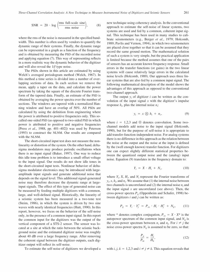
To extract the dynamic range as a function of frequencythe short-circuited time series are processed using equation(14) on recordings of 2 hr for the 100 samples/sec datastreams and 4 hr for 20 samples/sec data (Fig. 2). For fre-quencies above (roughly) 1 Hz the noise is flat and the PSDdoes not vary significantly with frequency. However below1 Hz the 1/f type of noise dominates and the dynamic rangedecreases at lower frequencies. The horizontal lines showtheoretical PSD levels for 22-, 23-, 24-, and 25-bit digitizersas derived from equation (7). The corresponding values for

the dynamic range of the digitizers are given on the rightaxes and follow from equation (5). The results in Figure 2show that for frequencies above (roughly) 1 Hz the dynamicrange for the three digitizers corresponds within a few deci-bels with the values in Table 1.

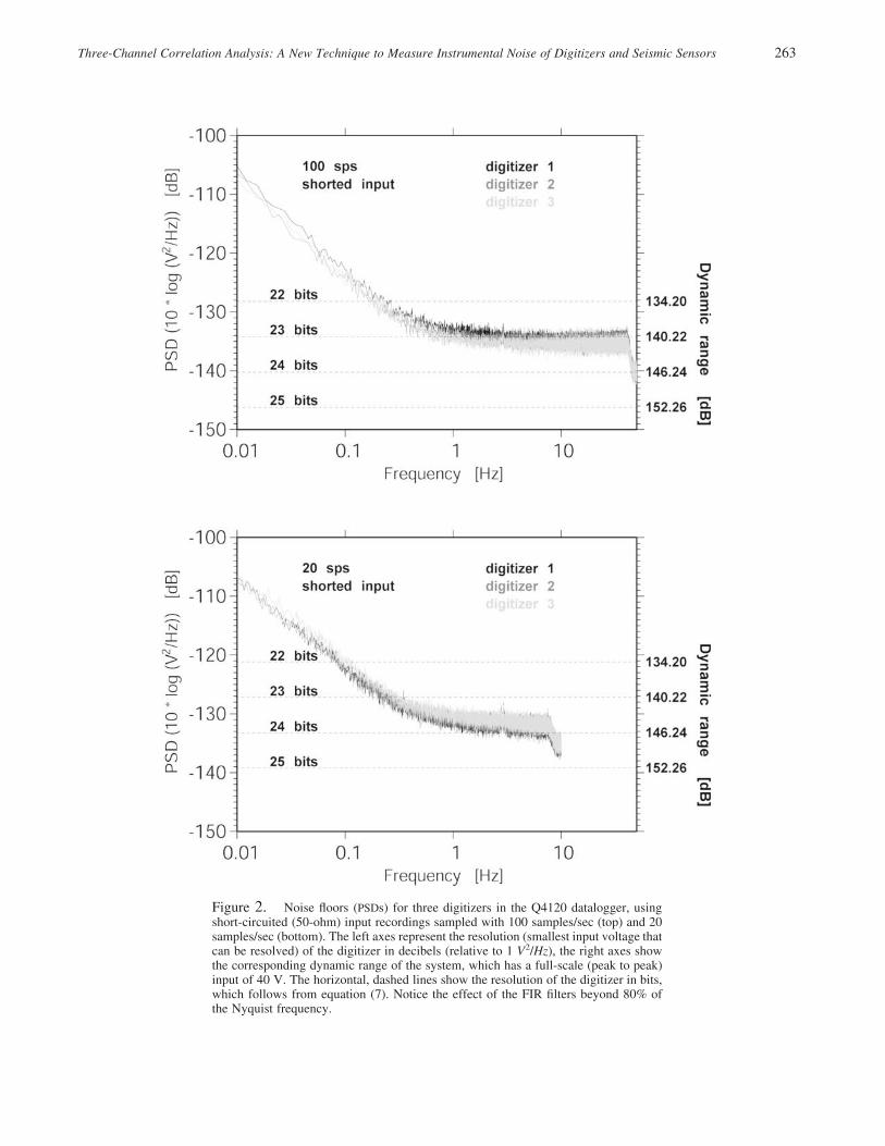
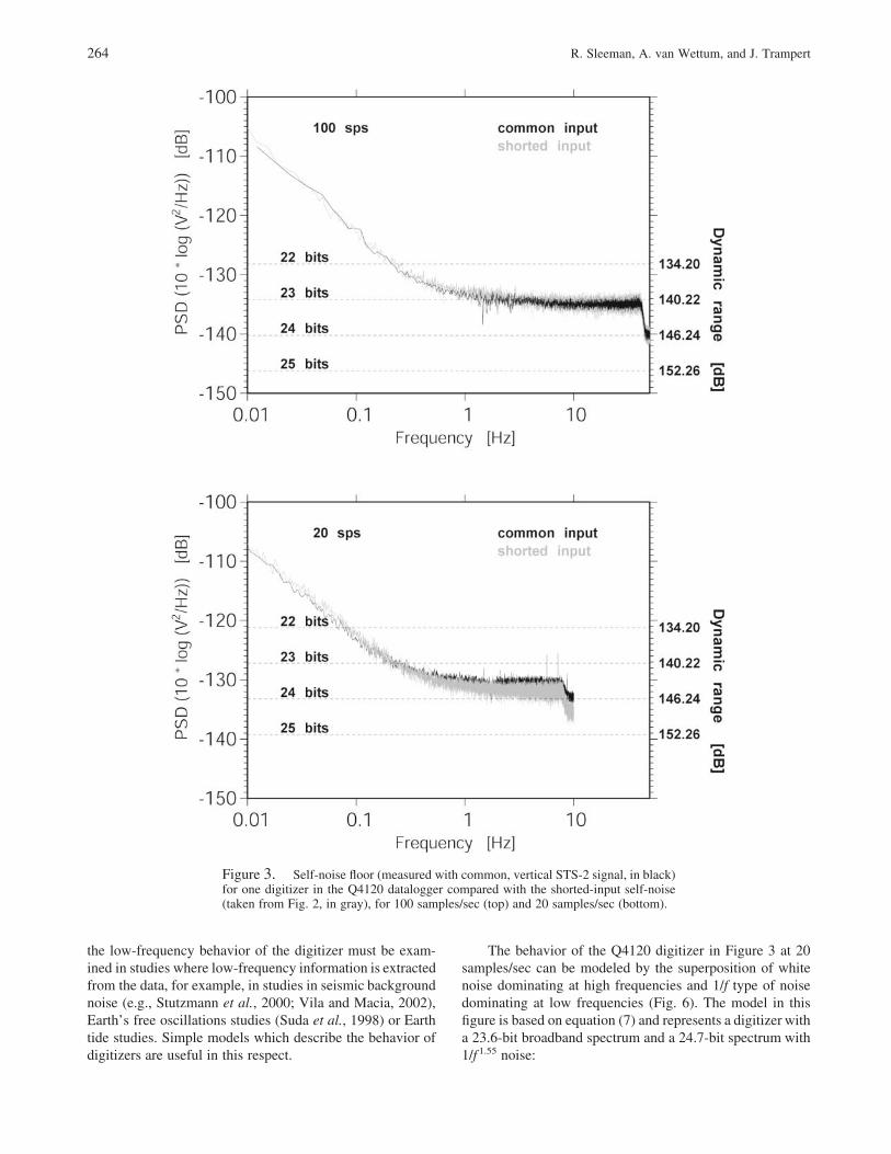
The effect of using a real seismic broadband signal onthe dynamic range is shown in Figure 3. The digitizer out-puts (recordings from the vertical component of an STS-2sensor) are processed by using equation (14) and the samewindow lengths as above. For the 100 samples/sec and 20samples/sec data the noise PSD of the shorted input mea-surement and the common input test are shown in gray andblack lines. Notice that only one digitizer is shown to seethe difference. At both sampling rates there is significantincrease in the self-noise level and hence no significant de-crease of the dynamic range. Figure 4 shows the measuredgain ratios between the digitizers in the Q4120 datalogger,smoothed over a tenth of a decade. Between 0.01 Hz and 8Hz, using data sampled with 20 samples/sec, the smoothedratios are within 1.6% (or 0.14 dB) of the values given bythe manufacturer.

These procedures are also applied to a NARS datalogger.The result of the coherency analysis on 20 samples/sec datais presented for one digitizer in Figure 5. Over the entirefrequency range (0.001–8 Hz) some additional self-noise isvisible, which decreases the dynamic range by a few deci-bels. At higher frequencies (1–8 Hz) the dynamic range in-creases to about 127 dB at 20 samples/sec, corresponding toa 20.8 bits digitizer. The PSD level at lower frequenciesshows a significant smaller slope as compared with theQ4120. For frequencies below 0.01 Hz the PSD level of theNARS datalogger is below the Q4120 PSD level.

Digitizer Noise Models

The dynamic behavior of the digitizers (Figs. 2 and 3)shows that the representation of the dynamic range by a sin-gle number is adequate for higher frequencies (above a fewhertz) but not for lower frequencies. Evidently, the effect of

Table 1Single Number Representation of the Dynamic Range (SNR) of

Three Digitizers in the Quanterra Q4120 Datalogger forSampling Rates of 1, 20, and 100 Samples/sec (sps)

SNR (dB)

DigitizerSensitivity(counts/V)

rms Full Scale(counts) 1 sps 20 sps 100 sps

CH 6 408,655 5,779,268 144.2 143.0 140.5CH 7 415,155 5,871,193 145.1 143.9 141.0CH 8 407,468 5,762,482 144.9 143.6 141.3

The dynamic range is calculated by applying equation (3) on a timeseries of 24 hr which was recorded with short-circuited (50-ohm) inputconnectors. The noise rms is calculated between 0.01 Hz and 80% of theNyquist frequency. The full-scale rms follows from the sensitivity valuesprovided by the manufacturer (Quanterra Inc.) and the full-scale input(40 V). CH � channel.


Figure 2. Noise floors (PSDs) for three digitizers in the Q4120 datalogger, usingshort-circuited (50-ohm) input recordings sampled with 100 samples/sec (top) and 20samples/sec (bottom). The left axes represent the resolution (smallest input voltage thatcan be resolved) of the digitizer in decibels (relative to 1 V2/Hz), the right axes showthe corresponding dynamic range of the system, which has a full-scale (peak to peak)input of 40 V. The horizontal, dashed lines show the resolution of the digitizer in bits,which follows from equation (7). Notice the effect of the FIR filters beyond 80% ofthe Nyquist frequency.


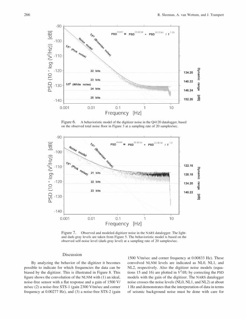
The behavior of the Q4120 digitizer in Figure 3 at 20samples/sec can be modeled by the superposition of whitenoise dominating at high frequencies and 1/f type of noisedominating at low frequencies (Fig. 6). The model in thisfigure is based on equation (7) and represents a digitizer witha 23.6-bit broadband spectrum and a 24.7-bit spectrum with1/f 1.55 noise:

the low-frequency behavior of the digitizer must be exam-ined in studies where low-frequency information is extractedfrom the data, for example, in studies in seismic backgroundnoise (e.g., Stutzmann et al., 2000; Vila and Macia, 2002),Earth’s free oscillations studies (Suda et al., 1998) or Earthtide studies. Simple models which describe the behavior ofdigitizers are useful in this respect.

Figure 3. Self-noise floor (measured with common, vertical STS-2 signal, in black)for one digitizer in the Q4120 datalogger compared with the shorted-input self-noise(taken from Fig. 2, in gray), for 100 samples/sec (top) and 20 samples/sec (bottom).


22A TPSD ( f ) � 10 • log •Q4120 � 23.6�� 2 6

22A T 1� • • (15)� 24.7� 1.55�2 6 f

(with T � 20 samples/sec, 2A � 40 V). Clearly the noise ofthe digitizer falls in between pink noise (1/f ) and Browniannoise (1/f 2). The interpretation for this behavior could be aseries of different processes with 1/f corner frequencies ofelectronic and thermal origin, that sum up to create an overallbehavior as observed (J.M. Steim, personal comm., 2004).

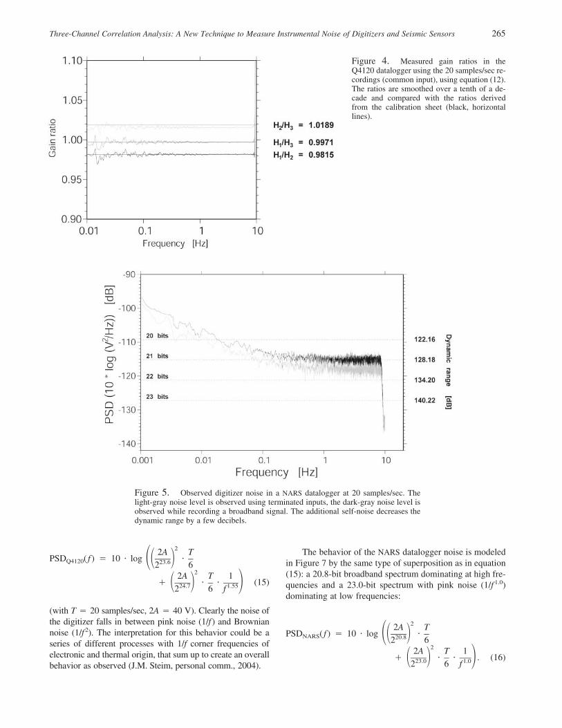
The behavior of the NARS datalogger noise is modeledin Figure 7 by the same type of superposition as in equation(15): a 20.8-bit broadband spectrum dominating at high fre-quencies and a 23.0-bit spectrum with pink noise (1/f 1.0)dominating at low frequencies:

22A TPSD ( f ) � 10 • log •NARS � 20.8�� 2 6

22A T 1� • • . (16)� 23.0� 1.0�2 6 f

Figure 4. Measured gain ratios in theQ4120 datalogger using the 20 samples/sec re-cordings (common input), using equation (12).The ratios are smoothed over a tenth of a de-cade and compared with the ratios derivedfrom the calibration sheet (black, horizontallines).

Figure 5. Observed digitizer noise in a NARS datalogger at 20 samples/sec. Thelight-gray noise level is observed using terminated inputs, the dark-gray noise level isobserved while recording a broadband signal. The additional self-noise decreases thedynamic range by a few decibels.


Discussion

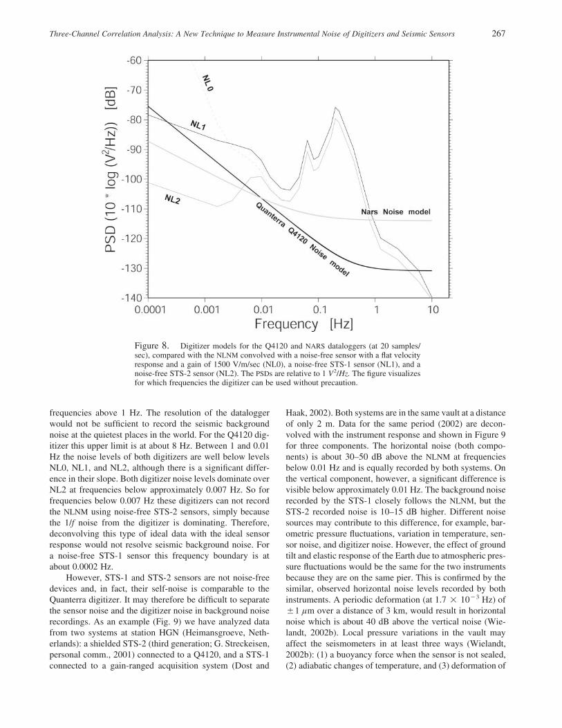
By analyzing the behavior of the digitizer it becomespossible to indicate for which frequencies the data can bebiased by the digitizer. This is illustrated in Figure 8. Thisfigure shows the convolution of the NLNM with (1) an ideal,noise-free sensor with a flat response and a gain of 1500 V/m/sec (2) a noise-free STS-1 (gain 2300 V/m/sec and cornerfrequency at 0.00277 Hz), and (3) a noise-free STS-2 (gain

1500 V/m/sec and corner frequency at 0.00833 Hz). Theseconvolved NLNM levels are indicated as NL0, NL1, andNL2, respectively. Also the digitizer noise models (equa-tions 15 and 16) are plotted in V2/Hz by correcting the PSDmodels with the gain of the digitizer. The NARS dataloggernoise crosses the noise levels (NL0, NL1, and NL2) at about1 Hz and demonstrates that the interpretation of data in termsof seismic background noise must be done with care for

Figure 6. A behavioristic model of the digitizer noise in the Q4120 datalogger, basedon the observed total noise floor in Figure 3 at a sampling rate of 20 samples/sec.

Figure 7. Observed and modeled digitizer noise in the NARS datalogger. The light-and dark-gray levels are taken from Figure 5. The behavioristic model is based on theobserved self-noise level (dark-gray level) at a sampling rate of 20 samples/sec.


frequencies above 1 Hz. The resolution of the dataloggerwould not be sufficient to record the seismic backgroundnoise at the quietest places in the world. For the Q4120 dig-itizer this upper limit is at about 8 Hz. Between 1 and 0.01Hz the noise levels of both digitizers are well below levelsNL0, NL1, and NL2, although there is a significant differ-ence in their slope. Both digitizer noise levels dominate overNL2 at frequencies below approximately 0.007 Hz. So forfrequencies below 0.007 Hz these digitizers can not recordthe NLNM using noise-free STS-2 sensors, simply becausethe 1/f noise from the digitizer is dominating. Therefore,deconvolving this type of ideal data with the ideal sensorresponse would not resolve seismic background noise. Fora noise-free STS-1 sensor this frequency boundary is atabout 0.0002 Hz.

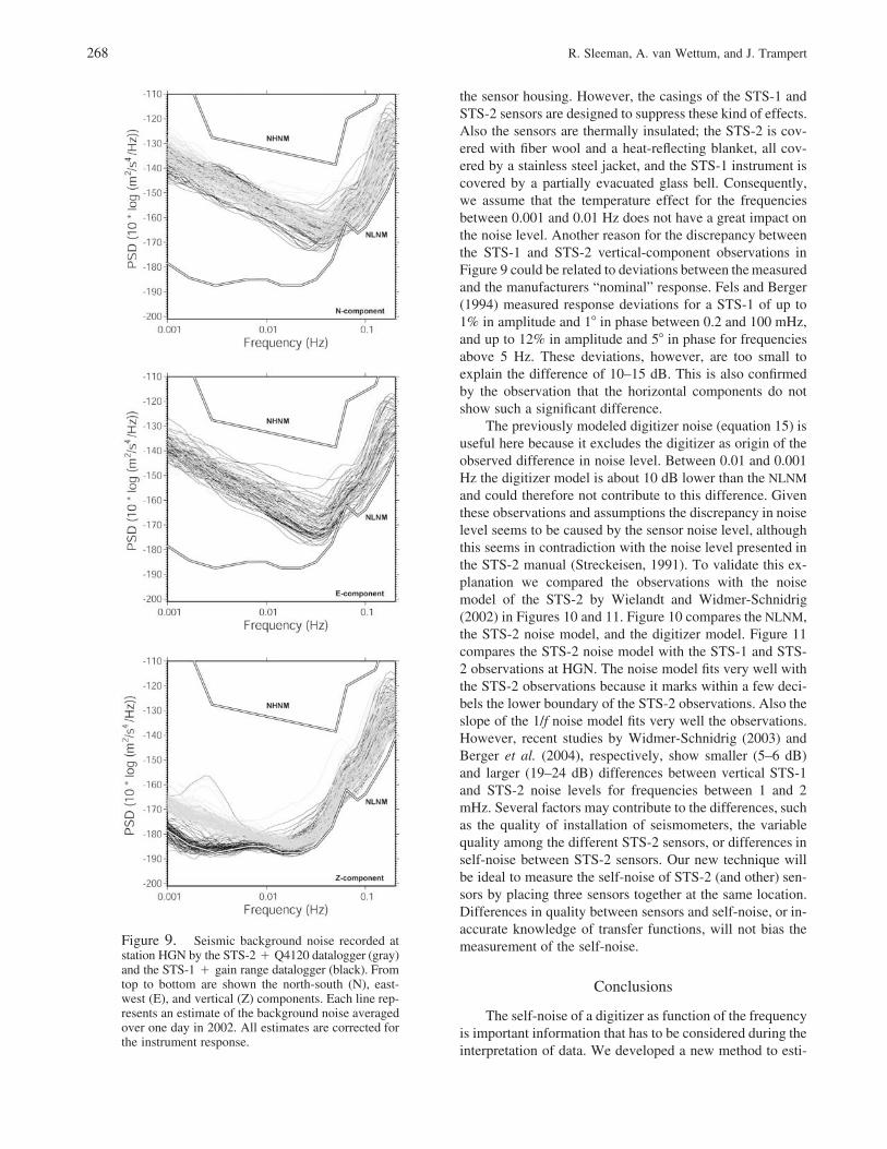
However, STS-1 and STS-2 sensors are not noise-freedevices and, in fact, their self-noise is comparable to theQuanterra digitizer. It may therefore be difficult to separatethe sensor noise and the digitizer noise in background noiserecordings. As an example (Fig. 9) we have analyzed datafrom two systems at station HGN (Heimansgroeve, Neth-erlands): a shielded STS-2 (third generation; G. Streckeisen,personal comm., 2001) connected to a Q4120, and a STS-1connected to a gain-ranged acquisition system (Dost and

Haak, 2002). Both systems are in the same vault at a distanceof only 2 m. Data for the same period (2002) are decon-volved with the instrument response and shown in Figure 9for three components. The horizontal noise (both compo-nents) is about 30–50 dB above the NLNM at frequenciesbelow 0.01 Hz and is equally recorded by both systems. Onthe vertical component, however, a significant difference isvisible below approximately 0.01 Hz. The background noiserecorded by the STS-1 closely follows the NLNM, but theSTS-2 recorded noise is 10–15 dB higher. Different noisesources may contribute to this difference, for example, bar-ometric pressure fluctuations, variation in temperature, sen-sor noise, and digitizer noise. However, the effect of groundtilt and elastic response of the Earth due to atmospheric pres-sure fluctuations would be the same for the two instrumentsbecause they are on the same pier. This is confirmed by thesimilar, observed horizontal noise levels recorded by bothinstruments. A periodic deformation (at 1.7 � 10�3 Hz) of�1 lm over a distance of 3 km, would result in horizontalnoise which is about 40 dB above the vertical noise (Wie-landt, 2002b). Local pressure variations in the vault mayaffect the seismometers in at least three ways (Wielandt,2002b): (1) a buoyancy force when the sensor is not sealed,(2) adiabatic changes of temperature, and (3) deformation of

Figure 8. Digitizer models for the Q4120 and NARS dataloggers (at 20 samples/sec), compared with the NLNM convolved with a noise-free sensor with a flat velocityresponse and a gain of 1500 V/m/sec (NL0), a noise-free STS-1 sensor (NL1), and anoise-free STS-2 sensor (NL2). The PSDs are relative to 1 V2/Hz. The figure visualizesfor which frequencies the digitizer can be used without precaution.


the sensor housing. However, the casings of the STS-1 andSTS-2 sensors are designed to suppress these kind of effects.Also the sensors are thermally insulated; the STS-2 is cov-ered with fiber wool and a heat-reflecting blanket, all cov-ered by a stainless steel jacket, and the STS-1 instrument iscovered by a partially evacuated glass bell. Consequently,we assume that the temperature effect for the frequenciesbetween 0.001 and 0.01 Hz does not have a great impact onthe noise level. Another reason for the discrepancy betweenthe STS-1 and STS-2 vertical-component observations inFigure 9 could be related to deviations between the measuredand the manufacturers “nominal” response. Fels and Berger(1994) measured response deviations for a STS-1 of up to1% in amplitude and 1� in phase between 0.2 and 100 mHz,and up to 12% in amplitude and 5� in phase for frequenciesabove 5 Hz. These deviations, however, are too small toexplain the difference of 10–15 dB. This is also confirmedby the observation that the horizontal components do notshow such a significant difference.

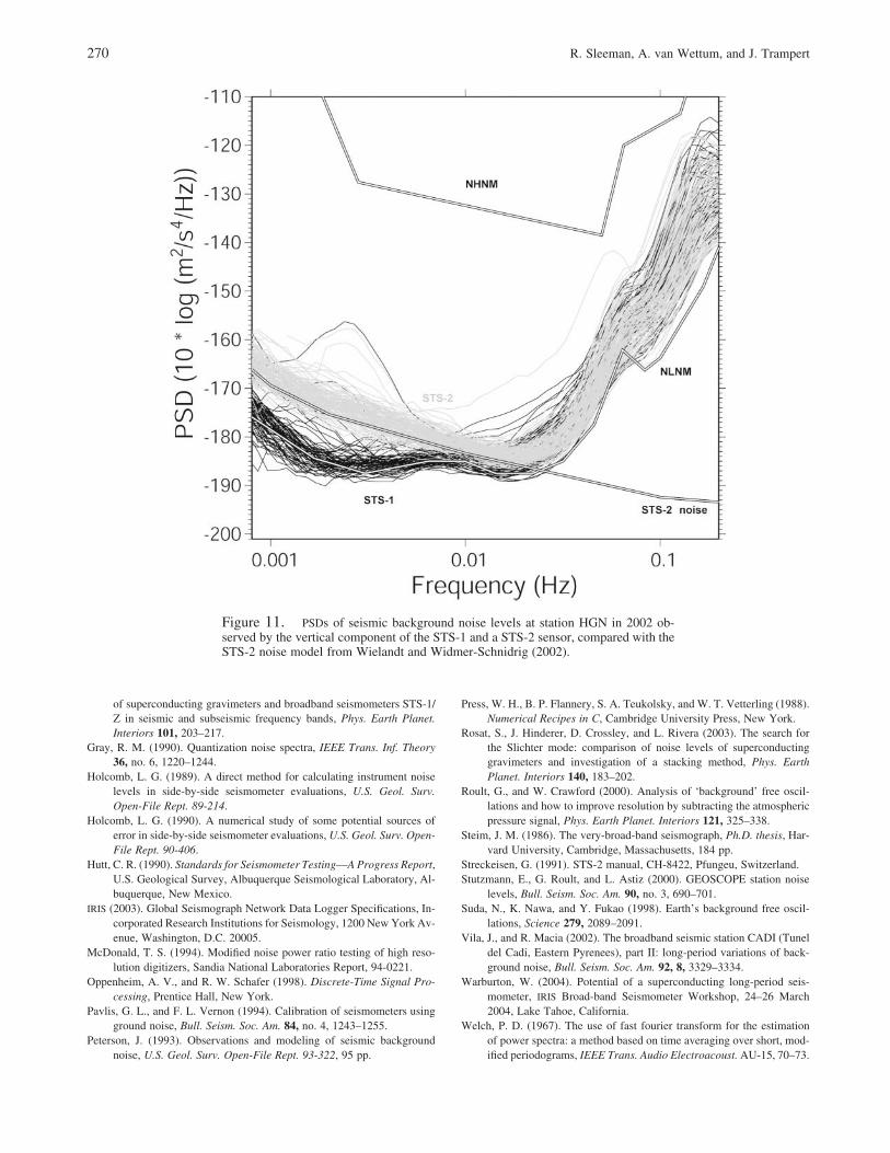
The previously modeled digitizer noise (equation 15) isuseful here because it excludes the digitizer as origin of theobserved difference in noise level. Between 0.01 and 0.001Hz the digitizer model is about 10 dB lower than the NLNMand could therefore not contribute to this difference. Giventhese observations and assumptions the discrepancy in noiselevel seems to be caused by the sensor noise level, althoughthis seems in contradiction with the noise level presented inthe STS-2 manual (Streckeisen, 1991). To validate this ex-planation we compared the observations with the noisemodel of the STS-2 by Wielandt and Widmer-Schnidrig(2002) in Figures 10 and 11. Figure 10 compares the NLNM,the STS-2 noise model, and the digitizer model. Figure 11compares the STS-2 noise model with the STS-1 and STS-2 observations at HGN. The noise model fits very well withthe STS-2 observations because it marks within a few deci-bels the lower boundary of the STS-2 observations. Also theslope of the 1/f noise model fits very well the observations.However, recent studies by Widmer-Schnidrig (2003) andBerger et al. (2004), respectively, show smaller (5–6 dB)and larger (19–24 dB) differences between vertical STS-1and STS-2 noise levels for frequencies between 1 and 2mHz. Several factors may contribute to the differences, suchas the quality of installation of seismometers, the variablequality among the different STS-2 sensors, or differences inself-noise between STS-2 sensors. Our new technique willbe ideal to measure the self-noise of STS-2 (and other) sen-sors by placing three sensors together at the same location.Differences in quality between sensors and self-noise, or in-accurate knowledge of transfer functions, will not bias themeasurement of the self-noise.

Conclusions

The self-noise of a digitizer as function of the frequencyis important information that has to be considered during theinterpretation of data. We developed a new method to esti-

Figure 9. Seismic background noise recorded atstation HGN by the STS-2 � Q4120 datalogger (gray)and the STS-1 � gain range datalogger (black). Fromtop to bottom are shown the north-south (N), east-west (E), and vertical (Z) components. Each line rep-resents an estimate of the background noise averagedover one day in 2002. All estimates are corrected forthe instrument response.


References

Aki, K., and P. G. Richards (1980). Quantitative Seismology, W. H. Free-man, San Francisco.

Baker, C. B. (1997). How to get 23 bits of effective resolution from your24-bit converter, Burr-Brown Application Bulletin, AB-120, Tucson,Arizona.

Beauduin, R., P. Lognonne, J. P. Montagner, S. Cacho, J. F. Karczewski,and M. Morand (1996). The effects of the atmospheric pressurechanges on seismic signals or how to improve the quality of a station,Bull. Seism. Soc. Am. 90, no. 4, 952–963.

Bennett, W. R. (1948). Spectra of quantized signals, Bell System Tec. J.27, 446–472.

Berger, J., D. C. Agnew, R. L. Parker, and W. E. Farell (1979). Seismicsystem calibration: 2. Cross-spectral calibration using random binarysignals, Bull. Seism. Soc. Am. 69, no. 1, 271–288.

Berger, J., P. Davis, and G. Ekstrom (2004). Ambient Earth noise: a surveyof the global seismographic network, J. Geophys. Res. 109, B11307.

Candy, C. J., and G. C. Temes (1992). Oversampling methods for A/D andD/A conversion, Oversampling Delta-Sigma Delta Converters, C. J.Candy and G. C. Temes (Editors), IEEE Press, Piscataway, NewJersey.

Clinton, J. F., and T. H. Heaton (2002). Performance of the VSE-355G2strong-motion velocity seismometer, Report to the IRIS-GSN subcom-mittee, California Institute of Technology.

Dost, B., and H. W. Haak (2002). A comprehensive description of theKNMI seismological instrumentation, Technical Report, TR-245,Koninklyk Nederlands Meteorologisch Instituut, De Bilt, Nether-lands.

Fels, J.-F., and J. Berger (1994). Parametric analysis and calibration of theSTS-1 seismometer of the IRIS/IDA seismographic network, Bull.Seism. Soc. Am. 84, no. 5, 1580–1592.

Freybourger, M., J. Hinderer, and J. Trampert (1997). Comparative study

mate instrumental noise in a three-channel, linear systembased on analysis of the output recordings only. The tech-nique can be applied to any datalogger or sensor in normalfield operation conditions. We applied the technique to aQ4120 datalogger and a NARS datalogger and modeled thebehavior of the self-noise level by only a few parametersdescribing resolution and 1/f noise. The two dataloggerstested here show significant differences in these parameters:at higher frequencies (above a few hertz) the resolution forthe Q4120 at 20 samples/sec is 23.8 bites, and 20.6 bits forthe NARS; the slope of the 1/f noise is 1.55 for the Q4120and 1.00 for the NARS. Also, the NARS datalogger showedsome additional self-noise, which is negligible in the Q4120.The usefulness of such models was shown in the interpre-tation of seismic background noise recorded at station HGNby an STS-1 and a STS-2. The digitizer model excludes thedigitizer noise to contribute to this difference. The differencein noise levels between those two instruments between 0.01and 0.001 Hz is in agreement with Wielandt and Widmer-Schnidrig (2002).

Acknowledgments

We thank Erhard Wielandt for his enthusiastic and constructive com-ments on this manuscript and the new technique in particular. Also thesuggestions and comments by R. Widmer-Schnidrig helped us to improvethe manuscript. All figures were generated using the software package GMT(Wessel and Smith, 1991).

Figure 10. STS-2 noise (Wielandt and Widmer-Schnidrig, 2002) compared withthe Q4120 noise and NL0 (see Fig. 8), by showing the corresponding PSDs relative to1 V2/Hz. For this purpose the STS-2 model is multiplied by 1500.


of superconducting gravimeters and broadband seismometers STS-1/Z in seismic and subseismic frequency bands, Phys. Earth Planet.Interiors 101, 203–217.

Gray, R. M. (1990). Quantization noise spectra, IEEE Trans. Inf. Theory36, no. 6, 1220–1244.

Holcomb, L. G. (1989). A direct method for calculating instrument noiselevels in side-by-side seismometer evaluations, U.S. Geol. Surv.Open-File Rept. 89-214.

Holcomb, L. G. (1990). A numerical study of some potential sources oferror in side-by-side seismometer evaluations, U.S. Geol. Surv. Open-File Rept. 90-406.

Hutt, C. R. (1990). Standards for Seismometer Testing—A Progress Report,U.S. Geological Survey, Albuquerque Seismological Laboratory, Al-buquerque, New Mexico.

IRIS (2003). Global Seismograph Network Data Logger Specifications, In-corporated Research Institutions for Seismology, 1200 New York Av-enue, Washington, D.C. 20005.

McDonald, T. S. (1994). Modified noise power ratio testing of high reso-lution digitizers, Sandia National Laboratories Report, 94-0221.

Oppenheim, A. V., and R. W. Schafer (1998). Discrete-Time Signal Pro-cessing, Prentice Hall, New York.

Pavlis, G. L., and F. L. Vernon (1994). Calibration of seismometers usingground noise, Bull. Seism. Soc. Am. 84, no. 4, 1243–1255.

Peterson, J. (1993). Observations and modeling of seismic backgroundnoise, U.S. Geol. Surv. Open-File Rept. 93-322, 95 pp.

Press, W. H., B. P. Flannery, S. A. Teukolsky, and W. T. Vetterling (1988).Numerical Recipes in C, Cambridge University Press, New York.

Rosat, S., J. Hinderer, D. Crossley, and L. Rivera (2003). The search forthe Slichter mode: comparison of noise levels of superconductinggravimeters and investigation of a stacking method, Phys. EarthPlanet. Interiors 140, 183–202.

Roult, G., and W. Crawford (2000). Analysis of ‘background’ free oscil-lations and how to improve resolution by subtracting the atmosphericpressure signal, Phys. Earth Planet. Interiors 121, 325–338.

Steim, J. M. (1986). The very-broad-band seismograph, Ph.D. thesis, Har-vard University, Cambridge, Massachusetts, 184 pp.

Streckeisen, G. (1991). STS-2 manual, CH-8422, Pfungeu, Switzerland.Stutzmann, E., G. Roult, and L. Astiz (2000). GEOSCOPE station noise

levels, Bull. Seism. Soc. Am. 90, no. 3, 690–701.Suda, N., K. Nawa, and Y. Fukao (1998). Earth’s background free oscil-

lations, Science 279, 2089–2091.Vila, J., and R. Macia (2002). The broadband seismic station CADI (Tunel

del Cadi, Eastern Pyrenees), part II: long-period variations of back-ground noise, Bull. Seism. Soc. Am. 92, 8, 3329–3334.

Warburton, W. (2004). Potential of a superconducting long-period seis-mometer, IRIS Broad-band Seismometer Workshop, 24–26 March2004, Lake Tahoe, California.

Welch, P. D. (1967). The use of fast fourier transform for the estimationof power spectra: a method based on time averaging over short, mod-ified periodograms, IEEE Trans. Audio Electroacoust. AU-15, 70–73.

Figure 11. PSDs of seismic background noise levels at station HGN in 2002 ob-served by the vertical component of the STS-1 and a STS-2 sensor, compared with theSTS-2 noise model from Wielandt and Widmer-Schnidrig (2002).


Wessel, P., and H. F. Smith (1991). Free software helps map and displaydata, EOS 72, 441.

Widmer-Schnidrig, R. (2003). What can superconducting gravimeters con-tribute to normal-mode seismology? Bull. Seism. Soc. Am. 93, no. 3,1370–1380.

Wielandt, E. (2002a). Seismometry, in International Handbook of Earth-quake and Engineering Seismology, Part A, W. H. K. Lee, H. Kan-amori, P. C. Jennings, and C. Kisslinger (Editors), Academic Press,San Diego, California, 283–304.

Wielandt, E. (2002b). Seismic sensors and their calibration, in IASPEI—New Manual of Seismological Observatory Practice, P. Bormann(Editor), GeoForschungsZentrum Potsdam, Potsdam, Germany.

Wielandt, E., and J. M. Steim (1986). A digital very-broad-band seismo-graph, Ann. Geophys. 4, B, no. 3, 227–232.

Wielandt, E., and R. Widmer-Schnidrig (2002). Seismic sensing and seis-mic noise, in Ten Years of German Regional Seismic Network(GRSN), Report 25 of the Senate Commission for Geosciences, M.Korn (Editor), Wiley-VCH Verlag GmbH, Weinheim, Germany.

Zurn, W., and R. Widmer (1995). On noise reduction in vertical seismic

records below 2 mHz using local barometric pressure, Geophys. Res.Lett. 22, no. 24, 3537–3450.

Royal Netherlands Meteorological Institute (KNMI)Seismology DivisionWilhelminalaan 103732 GK, De Bilt, [email protected]

(R.S.)

University of UtrechtFaculty of GeosciencesBudapestlaan 43584 CD, Utrecht, [email protected]@geo.uu.nl

(A.V.W., J.T.)

Manuscript received 23 February 2005.

three-channel correlation analysis: a new technique to ...seismain/pdf/bssa06-inst.pdf ·...

Documents