For permission to copy or republish, contact the American Institute of Aeronautics and Astronautics, 1801 Alexander Bell Drive, Suite 500, Reston, VA 20191

AIAA 2001-2171

Time Domain Simulations of Radiation from Ducted Fans with Liners

Yusuf Ozyoruk Middle East Technical University Ankara, Turkey Vineet Ahuja CRAFT Inc. Dublin, PA USA Lyle N. Long The Pennsylvania State University University Park, PA USA

7th AIAA/CEAS Aeroacoustics Conference 28 – 30 May 2001, Maastricht, The Netherlands

AIAA-2001-2171 1

TIME DOMAIN SIMULATIONS OF RADIATION

FROM DUCTED FANS WITH LINERS *

Y. Ozyoruk†† Middle East Technical University

Ankara, Turkey 06531

V. Ahuja† Combustion Research and Flow

Technology, Inc. Dublin, PA 18917 USA

L. N. Long§

Pennsylvania State University University Park, PA 16802

ABSTRACT*

Over the last few decades, noise related

concerns have played a major role in the development of aircraft engines. The previously dominant jet noise mechanisms are now being replaced by tonal and broadband noise from the fan and interactions from the fan wakes and the downstream stator. Alternately, engine inlet and exhaust ducts are being fitted with sophisticated liner materials that aid in damping fan related noise. In this paper, the authors investigate the radiation problem from the engine inlets with the aid of numerical simulations of the Euler/Navier-Stokes equations coupled with a time-domain methodology that analyzes the impedance characteristics of liner materials. In doing so, the authors present a simulation capability that can be used to identify and analyze tonal noise from high bypass ratio engines with acoustically treated nacelles. In this paper, we carry out numerical experiments and present results of radiation from two different engine inlet geometries with lined ducts.

1.0 INTRODUCTION

Over the past fifty years, air breathing propulsion technology for commercial and transport aircraft has evolved rapidly. Along with improving thrust and efficiency, reduction in engine noise has been one of the main criteria driving engine development. When the engine bypass ratio exceeds ten, fan noise replaces jet noise as the primary source of engine noise. Therefore, it is not surprising that extensive use of the high bypass ratio engine for commercial air transport has lead to a major focus in the reduction of fan related noise. This is a departure from the past, where efforts in reduction of engine noise were dominated by reduction in mixing noise/jet noise, turbine/combustor noise. The recent focus on fan noise lays emphasis on noise generating mechanisms and damping mechanisms such as the acoustic treatment of duct walls (liners). The noise

† Research Scientist, Senior Member AIAA. †† Associate Professor, Department of Aeronautical Engineering, Member AIAA. § Professor, Department of Aerospace Engineering, Associate Fellow AIAA. Copyright © 2001 by the authors. Published by AIAA with permission.

generating mechanisms in turbofan engines have been investigated and classified by Tyler and Sofrin [1] for quite some time now. They are generally attributed to spinning modes from the fan and the interaction of the rotor wakes with the stator blades downstream. Therefore, the aeroacoustics of high bypass ratio turbofan engines entails a detailed analysis of the turbomachinery systems, impact of the fluctuating pressure patterns on aerodynamic surfaces, transmission of the resultant modes in the inlet/exhaust ducts, interaction of the dominant modes with the liner material, and the prediction of farfield noise. Needless to say, a detailed analysis of the aeroacoustics of an engine represents a complex problem involving very disparate length and time scales, and physical mechanisms.

The tonal and broadband noise produced by the fan/turbomachinery travels in the nacelle and the exhaust duct before being radiated to the farfield. The tonal noise radiates based on cut-off values of the tones, shape of the nacelle and damping mechanisms associated with acoustic treatment of the ducts. The primary noise damping mechanism is the liner material embedded in the duct walls, which is responsible for impeding the tonal noise as it is transmitted through the exhaust duct/nacelle. Engines used today have sophisticated liners embedded along the duct walls. However, choice of an effective lining material is dependent on an accurate analysis of the sound produced in the nacelle/exhaust duct and the interaction of the liner material with the sound propagation characteristics.

Full scale simulations for the analysis of sound radiated from entire engine configurations including the liner presents many complexities. Firstly, high fidelity simulations of the liner and the engine body involves very disparate time and length scales. As a consequence, any generalized framework to carry out a coupled simulation will prove to be both complex and prohibitively expensive. As a result, most investigators explore the radiation problem from the engine using hard wall boundary conditions. In fact, most of the work in this area takes only the engine inlet into account. Many efficient boundary element [2,3] and finite element/wave-envelope [4] methods exist that have been used to provide efficient solutions of the radiation problems from the engine inlet with hard wall boundary assumptions. Furthermore, these methods fail to account for nonlinear effects, refraction from the nacelle and aerodynamic/aeroacoustic coupling. Advances in computational hardware have helped overcome some of the above-mentioned handicaps by

AIAA-2001-2171 2

permitting full 3-D Euler/Navier Stokes simulations utilizing high resolution schemes. The authors (Ozyoruk & Long [5,6]) have demonstrated simulation of forward radiation from the JT15D engine inlet with hard wall boundary assumptions. However, it has been observed that aft fan noise significantly contributes to engine noise. Furthermore, downstream radiation is further complicated by additional noise due to mixing in the shear layer at the aft end. Recently, the authors (Ahuja et al. [7]) extended the method to include both fore and aft radiation from a generic engine with hard wall boundaries. One of the main issues regarding aft fan noise has been to related accurate far-field sound prediction due to non-linear effects from the shear layer and the questionable use of a Kirchhoff surface. Long et al. [8] have shown that by using a Ffowcs Williams-Hawkings equation non-linear effects such as those generated by quadrupole source terms (e.g. in wakes) can be accounted for in far-field noise prediction.

Characterization of the acoustic impedance, and incorporating it in the engine noise radiation framework, is the second big challenge. The dissipative and resistive mechanisms inherent in resonant liners need to be identified and their interaction with engine tonal noise has to be simulated without resorting to Direct Numerical Simulations (DNS) type calculations. However, it must be mentioned that the authors recognize the value of microfluidic/DNS type simulations of liners in identifying and understanding the mechanisms by which the acoustic energy is dissipated in the vicinity of the liner orifice. In this paper, we are interested in a macroscopic characterization of the liner material and its response to the dominant acoustic modes produced in the engine.

Most liner materials resemble an ensemble of Helmholtz resonators with oscillatory jets that interact with the flow in the engine in a complex manner. In macroscopic terms, the engine lining material is characterized by an impedance value that consists of frequency dependent functions of the acoustic resistance and reactance typical of the material. This is primarily the reason that studies of engine liners in the past were limited to frequency domain methods. Additionally, analysis of broadband noise becomes increasingly difficult with such frequency domain methods. Recently, the authors (Ozyoruk & Long [9]) have devised a formulation for a frequency dependent impedance condition that can be used directly in time domain calculations. This methodology makes use of the z-transform, a concept used successfully in signal processing and electromagnetics. The authors have demonstrated (Ozyoruk & Long [10, 19]) with numerical solutions of the NASA Langley Research Center flow impedance tube, that this form of an impedance boundary condition coupled with Euler/Navier Stokes type solvers, can adequately simulate the effects of liner materials in engine inlet and exhaust ducts .

In this paper, we carry out numerical simulations of two different acoustically treated engine inlet configurations by solving the Euler/Navier-Stokes equations using a high resolution scheme. Farfield predictions are provided by an efficient implementation of the moving surface Kirchhoff formula of Farassat and Myers [11]. Our method has been previously used to predict sound for the JT15D engine inlet [5] with hard wall boundary conditions. These predictions have compared favorably with semi-analytical methods in predicting the BPF tones. Although the implementation in this paper is for nacelle ducts only, this approach is equally valid for the investigation of aft noise and acoustically treated exhaust ducts. Furthermore, the time-domain implementation of the impedance boundary condition allows for the possibility of investigation of broadband noise (provided that broadband noise sources such as turbulence/inlet disturbances/rotor interactions are accounted for). It is the purpose of this paper to investigate the effects of the liner on fore radiation of a generic engine configuration. In particular, we are interested in a dominant spinning mode (6,1) for this particular engine configuration and the reduction in sound pressure levels as a consequence of the liner material. The authors hope that with this paper a generalized framework for analyzing radiated rotor-stator tonal noise is laid out and it will take us a step closer to utilizing computational simulations in the design process and selection of acoustic materials that aid in reduction of fan related tonal noise. In the next section, we provide details of the numerical model including details of the time-domain impedance condition. In section 3, we discuss results of simulations of duct transmission and radiation from the JT15D engine inlet and a generic engine with lined ducts. The paper ends with concluding remarks and recommendations for future work.

2.0 NUMERICAL MODEL In this section we provide a brief overview of the numerical model that is being utilized to solve for sound propagation from full engine configurations with liner effects. We start with a discussion of the scheme being utilized to solve the Euler/Navier Stokes equations. A steady state solution is first computed for the mean flow. Multigrid acceleration is used for large residual reductions to ensure that no numerical noise corrupts the mean flow solution. The noise generating mechanisms i.e. rotor, rotor-stator interactions are not directly solved. The modes can be procured using a time-dependent solution by direct modeling of the fan blades or of the rotor and the stator in the engine of interest using a RANS based turbomachinery solver such as the ADPAC/CFL3D code [12,13]. In the present framework, either modes from the time-dependent simulations can be identified and incorporated or analytically specified as eigensolutions

AIAA-2001-2171 3

from infinite duct theory. For the prediction of farfield noise, the authors have utilized a Kirchhoff formulation. However, a severe limitation of this approach is that the Kirchhoff surface has to be located in a region of the flowfield devoid of any non-linear effects. This condition is easily satisfied in the investigation of sound from engine inlets [5] and is adequate for the purpose of this paper. Lastly, we discuss the impedance condition that is incorporated to model the liner effects. This is important because selection of the lining material and its installation requires detailed analysis of the sound fields of the engine inlet and exhaust ducts. Such analysis with liners has primarily been done only in the frequency domain [14], while time-domain studies included only hard-walled ducts. This is chiefly because the behavior of lining material is frequency dependent and an appropriate boundary condition in the time domain needs to be developed. Such a time-discrete form of the classical frequency dependent impedance condition is discussed, that establishes the critical link between the time and frequency domains utilizing the z-transform. 2.1 Interior Equations: Navier Stokes/Euler The 3-D time dependent Navier-Stokes/Euler equations are solved in body fitted generalized coordinates in the interior of the computational domain, with the non-reflecting boundary conditions solved on the outer boundaries. The spatial derivatives are computed using a fourth order stencil in each coordinate direction and gives significantly better dispersion and dissipation characteristics than second order schemes. Time integration is performed using a four stage Runge-Kutta method with a blend of Jameson’s [15] second and fourth order type artificial dissipation, for damping the spurious high wavenumber components. This scheme has a resolution of 12 cells per wavelength, is computationally economical. It has been adequately proven to be robust for aeroacoustic applications. The steady state solution is first computed and the solution is superposed with the driving unsteady source terms that replicate the effect of rotor-stator noise generating mechanisms. 2.2 Multigrid Convergence Acceleration Our approach is to utilize the full Euler/Navier-Stokes equations. However, in our simulations we do not directly solve for the noise generating mechanisms. Instead we procure a steady solution that represents the underlying mean flow, and analytically specify the noise generating mechanisms as part of our boundary condition procedure in the unsteady simulations. The resultant flowfields are a superposition of the unsteady dynamics on the steady state solution. Therefore, any spurious waves that are not damped out in the steady solution interfere with the acoustic pressure levels that are part of the unsteady simulation. Unfortunately, the very characteristics of low dispersion and dissipation, that are characteristic of high

resolution schemes and aid in accurate representation of wave propagation processes, hinder convergence to steady state. The convergence problem is alleviated in our method through the use of higher-order accurate multigrid acceleration, [16] wherein the low frequency numerical modes are aliased as high frequency modes on successive grids of varying coarseness. This is particularly attractive in acoustic problems with a mean flow, because of the high resolution nature of the grid that is needed to resolve acoustic frequencies of interest. Convergence to a steady state is typically extremely slow on such highly packed grids due to a broader spectrum of low frequency errors. Furthermore, it has been our experience that in the case of complex geometries, especially those with multiple corner points, trailing edges etc., the coarse grids need to be generated carefully, in order to retain these defining features of the geometries that are critical to the flow. Since the coarse grid is an outcome of coarsening the finest grid, these geometrical constraints have to be accounted for during the initial grid generation stage. In our implementation we have used Jameson’s full approximation scheme [17] with a 3 level V-cycle formulation. We have found the scheme to be robust and very efficient in driving convergence to machine accuracy.

2.3 Fan Face Conditions The steady part of the solution at the fan face is obtained using characteristic boundary conditions. These conditions drive the local variables to some mean values at the fan stage which are determined a priori based on gas dynamic relationships using information related to the operating conditions of the engine such as the mass flow rate and the free-stream Mach number. The unsteady acoustic pressure is superimposed on the steady solution with the aid of source terms. These source terms simulate the effect of the sound generating mechanisms involving rotor-stator interactions and are derived from infinite duct theory. These source terms could also come from experimental data. This data can be converted to modal data to produce source terms for the solver. Alternately, we could also carry out high fidelity simulations of the rotor and stator blade rows from traditional turbomachinery CFD codes, which could accurately predict the dominant modes but cannot accurately propagate the sound. Duct acoustic modes representing the circumferential and radial modes are specified. The circumferential mode is related to the number of stator vanes and rotor blades. An analysis of the cut-off ratios for each particular mode is carried out to determine all active modes. Summation over all the eigensolutions corresponding to all active modes gives us a representative source term that can be specified at the fan face. The source terms that simulate the effect of the sound generating mechanisms involving rotor-stator interactions are derived from infinite duct theory. Duct

AIAA-2001-2171 4

acoustic modes are classified as (m, µ) representing the circumferential and radial modes. The circumferential mode is related to the number of stator vanes and rotor blades through the relation

m = n B + sV s=…-2,-1,0,1,2… The acoustic pressure in an infinite cylinder as a function of (r, θ, x) is given as

ˆ p nmµ x, r,θ,( )= A nmµJm kmµ r( )

exp i kx,mµ x + mθ + φnmµ( )[ ]

A summation over all the eigensolutions corresponding to all active modes gives us a representative source term that can be specified at the fan face

( )

=θ′ ∑ ∑ ∑

∞

=

∞

−∞=

∞

=µ

ω−µ

1n m 0

ntinmf epRt,,r,xp

The axial wave number kx,mµ is given by

kx,mµ =−Mf k − k2 − 1 − M f

2( )km,µ2

1− Mf2

And the axial wavelength λa = 2πkx,mµ

with the sign of

kx,mµ determining upstream or downstream travelling wave. The cut-off ratio of a particular mode (m,µ) is given by

ξmµ =nBMT

rf kmµ 1− Mf2

where MT is the rotor tip speed. For the cases of no mass flow through the duct, velocity perturbations are specified at the fan face. These perturbations are obtained conveniently by substituting the exact acoustic pressure expression into the momentum equations. The momentum source terms are specified based on the linearized momentum equations and the acoustic pressure obtained from cylindrical duct theory and are listed here for sake of convenience.

ρ ˆ u 1( )nmµ = ρ∞ ℜkx,mµρ∞nω

′ p nmµ

ρ ˆ u 2( )nmµ = ρ∞ℜkmµ

ρ∞nω

′ J m kmµr( )Jm kmµr( ) ′ p nmµ

ρ ˆ u 3( )nmµ = ρ∞ ℜm

ρ∞ nωr′ p nmµ

( )

ρ=θρ ω−

µ

∞

=

∞

=µ∑∑ ∑ nti

nm1n m 0

ii e)u(R)t,,r,x(u

2.4 Kirchhoff Formulation and Farfield Conditions Limitations on computational resources preclude

the extension of the computational domain into the far-field. The acoustic response in the near-field is bridged by means of the Kirchhoff formula [15] of Farassat and Myers [7] to the far-field. This formulation of the Kirchhoff integration surface is for arbitrarily moving and deforming surfaces and is coupled with our Euler-Navier Stokes solver. Implementation on a distributed computing environment is performed by letting each processor identify that part of the Kirchhoff surface which is located in its computational domain. Before the time integration process begins, the time delay associated with each element is calculated and a global minimum is communicated to each processor. This marks the starting point of the acoustic pressure storage array on all processors. During the iterative process, each processor sums the contributions of acoustic pressure from the elements in its computational domain. After the simulation, the acoustic pressure arrays from all processors are summed up to get the final response in the farfield. Further details of the implementation can be found in Refs[5] and [6].

Since calculations are carried out on a truncated computational domain, it is imperative that the farfield boundary conditions minimize reflections of waves traveling out of the domain. The boundary conditions proposed by Bayliss and Turkel [20] have been incorporated in the code. These non-reflecting boundary conditions have been recast in a consistent form with the interior equations, thereby making the flux evaluation and time integration process streamlined for parallel computations.

2.5 Time-Discrete Impedance Condition Traditionally, the acoustic impedance condition has been limited to frequency domain methods, primarily because of the frequency dependent characteristics of lining materials. Time domain applications of such materials are difficult to simulate because of the computation of expensive convolutions. In this section we present a methodology to efficiently account for the lining material in the time domain using a digital signal processing concept involving the z-transform. In particular, the z-transform eases the computational burden associated with convolutions. For example, let us

AIAA-2001-2171 5

consider the impedance condition in the absence of mean flow:

)(/)(ˆ).( wZwpnwV a−=&

& and

)()()( wiXwRwZ +=

here R(w) and X(w) are the frequency dependent resistance and reactance respectively, used in the definition of the impedance Z(w). V(w) is the complex amplitude of the velocity perturbation, and pa is the pressure perturbation. In the time-domain the pressure perturbation can be expressed as

τττ dVntZtpt

a )(.)()(ˆ0

&

&

∫ −−=

however, the impedance must now be expressed in the time domain and the past history of the normal velocity perturbation at the wall must be provided in order to evaluate the integral. One could consider the convolution integral as the acoustic system’s response to the normal velocity input and the integrals as the output. The aim is to represent the discrete form of the output as a linear combination of inputs and outputs. The z-transform aids in expressing the convolution summation as an equivalent finite series. The impedance Z can now be expressed as a fraction of two finite polynomials in the complex variable z. By utilizing the inverse z-transform and a shifting theorem, analogous to the one used in Fourier transforms, the perturbation pressure can be expressed in the Z domain as )()()( zVzZzP na −=

Here

22

11

110

1)( −−

−

−−+

=zbzb

zaazZ

here a’s and b’s are some constants. By utilizing the inverse z-transform and a shifting theorem, analogous to the one used in Fourier transforms, the perturbation pressure can be expressed in the time domain as

)( 100

22

11

−−− +−+= nn

nn

na

na

na vavapbpbp

In the presence of mean flow a comparable boundary condition can be derived and coupled to the interior equations. The acoustic impedance condition is applied by allowing the fluid to slip at the wall with the liner boundary condition. This essentially corresponds to a zero thickness acoustic boundary layer assumption when the background flow is sheared. A non-zero normal velocity exists at the liner and the same equations as the interior flow are solved for the velocity components. The energy equation is replaced by an equation for the impedance condition. This equation updates the acoustic pressure perturbation based on the gradient of the velocity perturbation and a source term that is related to the z-transform of the functional form of the frequency dependent impedance data. This impedance data refers to experimentally obtained resistance and reactance

characteristics in frequency space of the liner material. Details of the transformation and the implementation are provided in Ozyoruk &Long [9], although a condensed version of the condition and its implementation is provided below. Acoustic impedance condition is applied on acoustically treated surfaces (liner). Because fluid particles are allowed to slip at a wall and because there is in general fluid penetration into an acoustic treatment element (i.e. non-zero normal velocity exists), we solve the same equations as the interior for the velocity components but replace the energy equation with the impedance condition equation, whose time-discrete form is given as

na

nna

nna

na

na

na Rtvvaptpp −∆−−=+∆− +++ /)(/)( ,

1,0

10

1"

as disscussed in [9]. The interior solution scheme and the time-discrete impedance condition are coupled through the linearized momentum equation written at the wall as

01

.. 0200

0,0,, =

∂∂

−∂∂

+−−++∂

∂n

p

n

pnvnvvv

t

v aaaanana

na

ρρ

ρ&

"&

"&

""

nv ,0& is the normal component of the mean velocity,

∇= .0v&

" , a"

is the perturbed equivalent of " . 0ρ is

the mean density, and aρ is the density perturbation. The

tangential velocity perturbation and the density perturbation are extrapolated from the interior equations once they are available from the integration of the interior equations. This sets the stage to evaluate the normal velocity perturbations and the pressure perturbations at the wall using the impedance conditions delineated above.

3.0 DISCUSSION OF RESULTS The numerical methodology discussed in the previous section has been utilized in investigations of radiation from two different configurations of engine inlets with mass flow and acoustic treatment of the duct walls. The computer codes used in these simulations are written in Fortran 90 combined with Message Passing Interface libraries. The codes are portable across a variety of parallel platforms. It must be mentioned that this is a departure from our previous codes which were written in CM-Fortran and their utility was limited to Connection machines. In Section 3.1 we look at fore radiation from the JT15D engine with and without mass flow and the impact of the liner material as an effective damping mechanism. This is followed by Section 3.2 where we discuss radiation from the nacelle of a generic engine configuration including a centerbody. In particular, there is considerable interest in the spinning modes that are transmitted through the lined ducts in this case.

AIAA-2001-2171 6

Figure 2. Acoustic Pressure Levels with and without liner for the JT15D Engine Inlet with no mass flow.

Figure 1. Schematic showing different liner positions for the JT15D engine inlet.

Figure 3. Far-field sound pressure levels and directivity showing impact of liner placement at 1 BPF, 2 BPF, 3BPF and 4BPF.

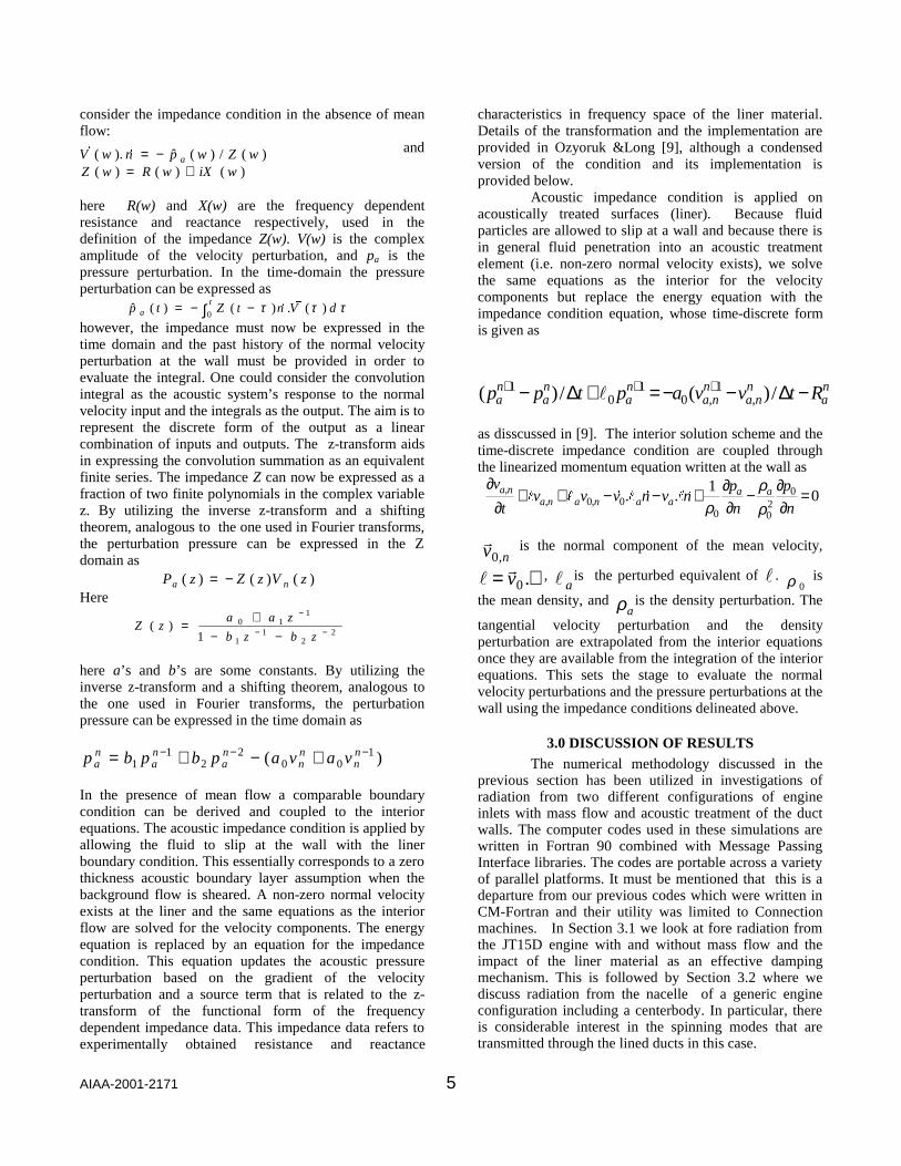
3.1 Radiation of (0,0) +(0,1) Modes Without Mass Flow and Acoustic Treatment for JT15D Inlet In this section we discuss axisymmetric simulations pertaining to the JT15D engine inlet with acoustic treatment of the walls and without mass flow. The liner impedance is shown in Table 1 for the frequencies of interest.

(Frequency kHz) Z/(ρ0c0)

0.5 0.406 – 1.587i 1.0 0.476 + 0.113i 1.5 1.078 + 1.638i 2.0 5.009 – 0.276i 2.1 4.008 – 1.601i

Liner pos.2

13

Fan

This simulation involved radiation of the plane wave modes (0,0) and (0,1) combined up to the 4th harmonic of the blade passage frequency. A 180 degree phase difference is introduced between the (0,0) and (0,1) modes of each harmonic and the total acoustic pressure amplitude for each pair is selected to carry a sound pressure level of 120 dB at the rotor blade tips. The blade passage frequency is chosen at 0.5 kHz so that the highest resolution of 2.0 kHz does not exceed the resolution requirements for the mesh. At these conditions only the (0,1) mode at the blade passage frequency is cut-off. Three different liner locations are shown for comparison purposes in the schematic in Fig. 1. The effect of the acoustic treatment is visible from Fig. 2, where a back-to-back comparison is made with a case without the liner material and the liner in position 1. There is a strong focusing of the waves towards the centerline.

When compared with the hard-wall case the generation of some additional modes over the liner is observed. These modes propagate in both the upstream and downstream directions. The Kirchhoff surface integration results for the far-field noise are displayed in

Fig. 3 for each harmonic of the fundamental frequency. Since the (0,1) mode is cut-off at 1 BPF, the sound pressure level (SPL) curves do not show any wave reinforcements or cancellations at the far-field at this frequency. It is evident from Fig. 3 that liner position 3 is the best location for absorbing noise at this frequency. All liner locations yield some reduction in SPL in a region from 40 degrees from the inlet axis upstream for the 2 BPF case. However, there is an increase in SPL between 40 and 150 degrees from the upstream axis. The most significant change is obtained for the liner material at position 2. As the frequency increases, more pronounced lobes are seen with liner 2 position yielding significant

20

40

60

80 Hard wallLiner, pos. 1position 2position 3

1 BPF = 500 Hz

θ=30o150o

20

40

60

80 Hard wallLiner, pos. 1position 2position 3

2 BPF

Sound PressureLevel, dB80 60 40 20 0 20 40 60 80

20

40

60

80 Hard wallLiner, pos. 1position 2position 3

3 BPF

Sound PressureLevel, dB80 60 40 20 0 20 40 60 80

20

40

60

80 Hard wallLiner, pos. 1position 2position 3

4 BPF

Table 1. Impedance values used.

AIAA-2001-2171 7

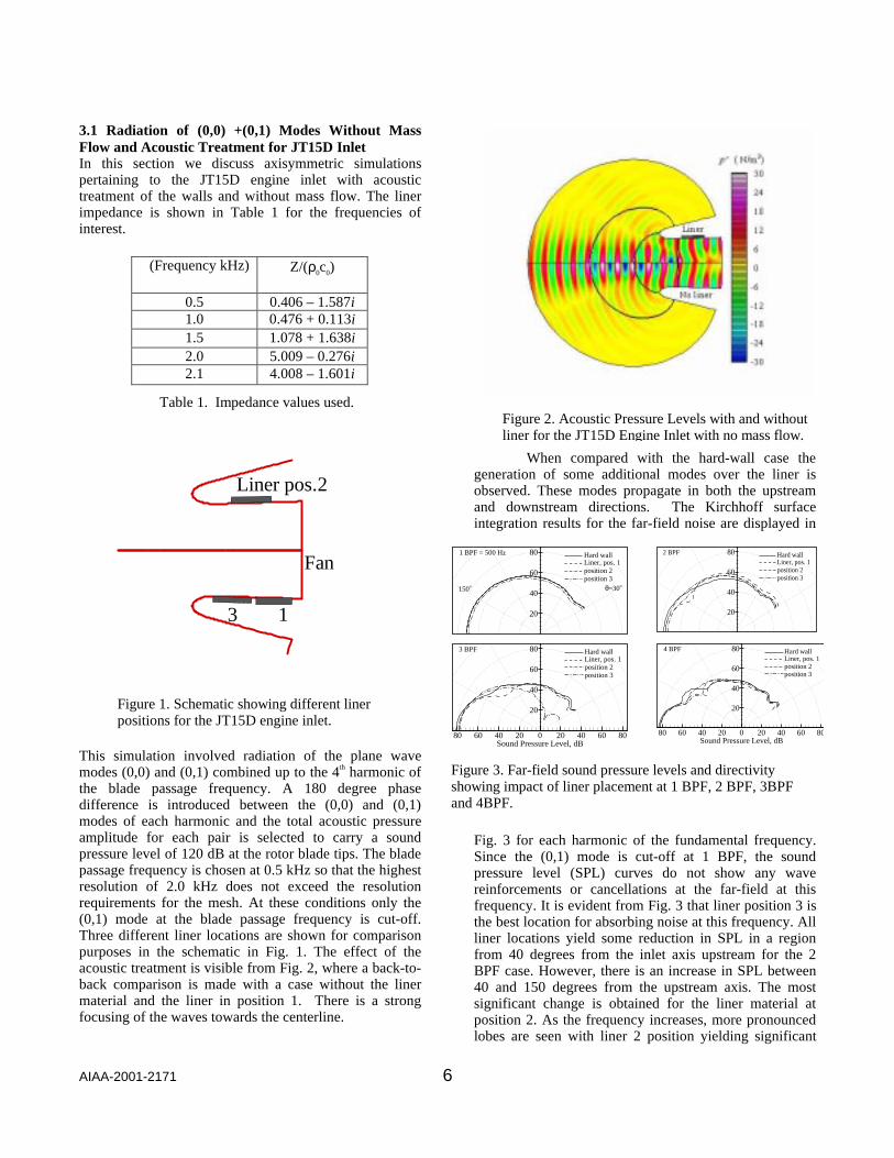
Figure 4. Instantaneous acoustic pressure levels with liner material. The steady state pressure field is depicted in the lower half.

Figure 5. Farfield sound pressure levels for the JT15D engine inlet with liner and mass flow

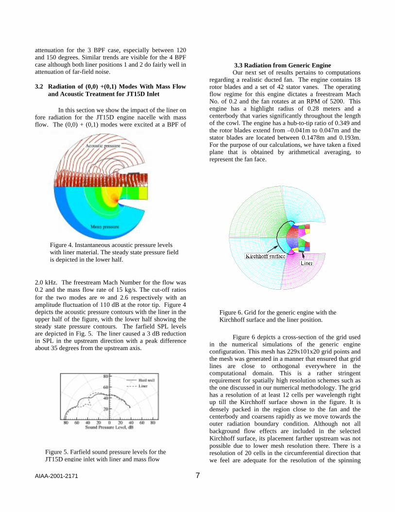
Figure 6. Grid for the generic engine with the Kirchhoff surface and the liner position.

attenuation for the 3 BPF case, especially between 120 and 150 degrees. Similar trends are visible for the 4 BPF case although both liner positions 1 and 2 do fairly well in attenuation of far-field noise.

3.2 Radiation of (0,0) +(0,1) Modes With Mass Flow

and Acoustic Treatment for JT15D Inlet In this section we show the impact of the liner on fore radiation for the JT15D engine nacelle with mass flow. The (0,0) + (0,1) modes were excited at a BPF of

2.0 kHz. The freestream Mach Number for the flow was 0.2 and the mass flow rate of 15 kg/s. The cut-off ratios for the two modes are ∞ and 2.6 respectively with an amplitude fluctuation of 110 dB at the rotor tip. Figure 4 depicts the acoustic pressure contours with the liner in the upper half of the figure, with the lower half showing the steady state pressure contours. The farfield SPL levels are depicted in Fig. 5. The liner caused a 3 dB reduction in SPL in the upstream direction with a peak difference about 35 degrees from the upstream axis.

3.3 Radiation from Generic Engine Our next set of results pertains to computations

regarding a realistic ducted fan. The engine contains 18 rotor blades and a set of 42 stator vanes. The operating flow regime for this engine dictates a freestream Mach No. of 0.2 and the fan rotates at an RPM of 5200. This engine has a highlight radius of 0.28 meters and a centerbody that varies significantly throughout the length of the cowl. The engine has a hub-to-tip ratio of 0.349 and the rotor blades extend from –0.041m to 0.047m and the stator blades are located between 0.1478m and 0.193m. For the purpose of our calculations, we have taken a fixed plane that is obtained by arithmetical averaging, to represent the fan face.

/LQHU

.LUFKKRII VXUIDFH

Figure 6 depicts a cross-section of the grid used in the numerical simulations of the generic engine configuration. This mesh has 229x101x20 grid points and the mesh was generated in a manner that ensured that grid lines are close to orthogonal everywhere in the computational domain. This is a rather stringent requirement for spatially high resolution schemes such as the one discussed in our numerical methodology. The grid has a resolution of at least 12 cells per wavelength right up till the Kirchhoff surface shown in the figure. It is densely packed in the region close to the fan and the centerbody and coarsens rapidly as we move towards the outer radiation boundary condition. Although not all background flow effects are included in the selected Kirchhoff surface, its placement farther upstream was not possible due to lower mesh resolution there. There is a resolution of 20 cells in the circumferential direction that we feel are adequate for the resolution of the spinning

AIAA-2001-2171 8

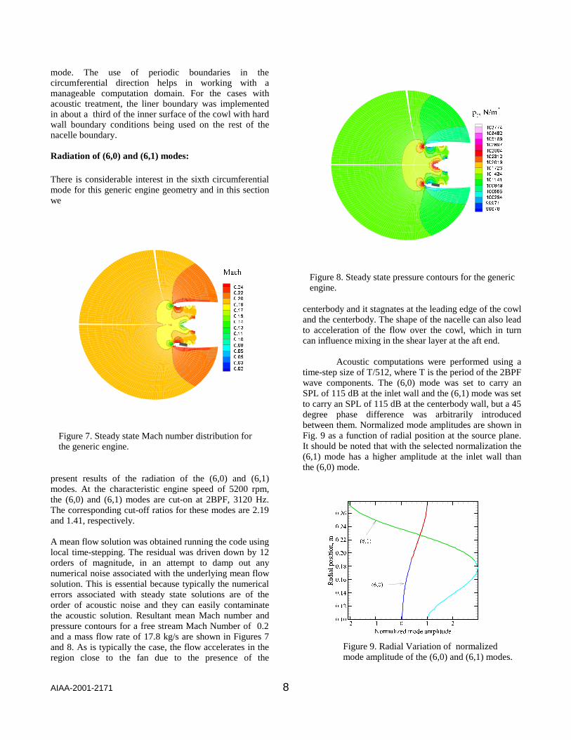
Figure 7. Steady state Mach number distribution for the generic engine.

Figure 8. Steady state pressure contours for the generic engine.

Figure 9. Radial Variation of normalized mode amplitude of the (6,0) and (6,1) modes.

mode. The use of periodic boundaries in the circumferential direction helps in working with a manageable computation domain. For the cases with acoustic treatment, the liner boundary was implemented in about a third of the inner surface of the cowl with hard wall boundary conditions being used on the rest of the nacelle boundary.

Radiation of (6,0) and (6,1) modes: There is considerable interest in the sixth circumferential mode for this generic engine geometry and in this section we

����

����

����

����

����

����

����

����

����

����

����

����

����

����

����

0DFK

present results of the radiation of the (6,0) and (6,1) modes. At the characteristic engine speed of 5200 rpm, the (6,0) and (6,1) modes are cut-on at 2BPF, 3120 Hz. The corresponding cut-off ratios for these modes are 2.19 and 1.41, respectively. A mean flow solution was obtained running the code using local time-stepping. The residual was driven down by 12 orders of magnitude, in an attempt to damp out any numerical noise associated with the underlying mean flow solution. This is essential because typically the numerical errors associated with steady state solutions are of the order of acoustic noise and they can easily contaminate the acoustic solution. Resultant mean Mach number and pressure contours for a free stream Mach Number of 0.2 and a mass flow rate of 17.8 kg/s are shown in Figures 7 and 8. As is typically the case, the flow accelerates in the region close to the fan due to the presence of the

������

������

������

������

������

������

������

������

������

������

������

������

������

�����

�����

S�� 1�P

�

centerbody and it stagnates at the leading edge of the cowl and the centerbody. The shape of the nacelle can also lead to acceleration of the flow over the cowl, which in turn can influence mixing in the shear layer at the aft end. Acoustic computations were performed using a time-step size of T/512, where T is the period of the 2BPF wave components. The (6,0) mode was set to carry an SPL of 115 dB at the inlet wall and the (6,1) mode was set to carry an SPL of 115 dB at the centerbody wall, but a 45 degree phase difference was arbitrarily introduced between them. Normalized mode amplitudes are shown in Fig. 9 as a function of radial position at the source plane. It should be noted that with the selected normalization the (6,1) mode has a higher amplitude at the inlet wall than the (6,0) mode.

1RUPDOL]HG PRGH DPSOLWXGH

5DG

LDOSRVLWLRQ�P

�� �� � � �����

����

����

����

����

����

����

����

����

�����

�����

AIAA-2001-2171 9

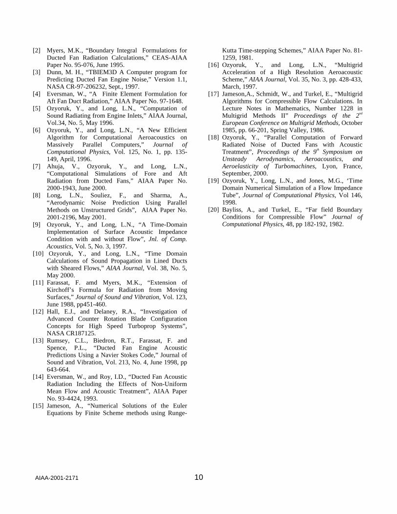
Figure 10. Instantaneous acoustic pressure levels showing the (6,0) and (6,1) spinning modes without liner(upper half) and with liner(lower half) for the generic engine inlet.

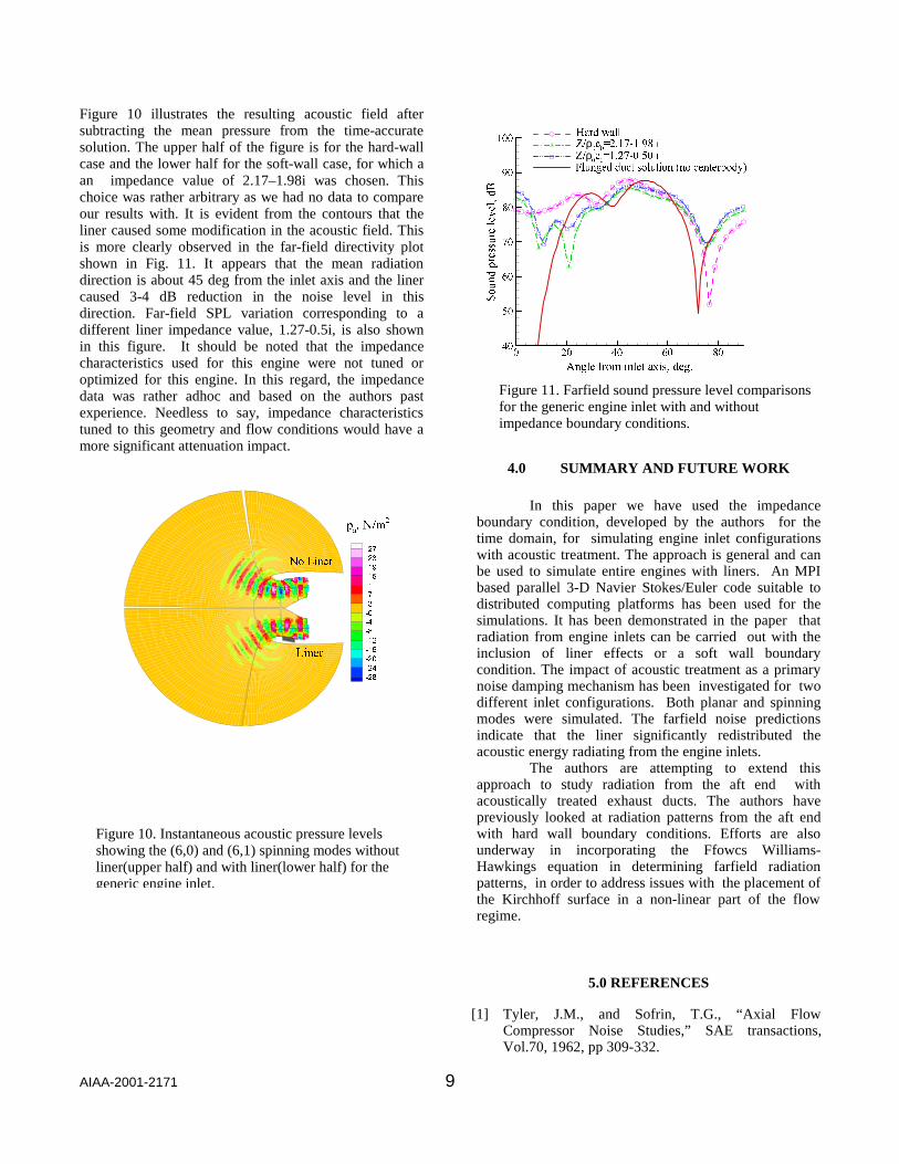
Figure 11. Farfield sound pressure level comparisons for the generic engine inlet with and without impedance boundary conditions.

Figure 10 illustrates the resulting acoustic field after subtracting the mean pressure from the time-accurate solution. The upper half of the figure is for the hard-wall case and the lower half for the soft-wall case, for which a an impedance value of 2.17–1.98i was chosen. This choice was rather arbitrary as we had no data to compare our results with. It is evident from the contours that the liner caused some modification in the acoustic field. This is more clearly observed in the far-field directivity plot shown in Fig. 11. It appears that the mean radiation direction is about 45 deg from the inlet axis and the liner caused 3-4 dB reduction in the noise level in this direction. Far-field SPL variation corresponding to a different liner impedance value, 1.27-0.5i, is also shown in this figure. It should be noted that the impedance characteristics used for this engine were not tuned or optimized for this engine. In this regard, the impedance data was rather adhoc and based on the authors past experience. Needless to say, impedance characteristics tuned to this geometry and flow conditions would have a more significant attenuation impact.

��

��

��

��

��

�

�

��

��

��

���

���

���

���

���

1R /LQHU

/LQHU

SD� 1�P

�

$QJOH IURP LQOHW D[LV� GHJ�

6RXQGSUHVVXUH

OHYHO�G%

� �� �� �� ����

��

��

��

��

��

���+DUG ZDOO

)OXQJHG GXFW VROXWLRQ �QR FHQWHUERG\�

=�ρ�F� ��������� L

=�ρ�F� ��������� L

4.0 SUMMARY AND FUTURE WORK

In this paper we have used the impedance boundary condition, developed by the authors for the time domain, for simulating engine inlet configurations with acoustic treatment. The approach is general and can be used to simulate entire engines with liners. An MPI based parallel 3-D Navier Stokes/Euler code suitable to distributed computing platforms has been used for the simulations. It has been demonstrated in the paper that radiation from engine inlets can be carried out with the inclusion of liner effects or a soft wall boundary condition. The impact of acoustic treatment as a primary noise damping mechanism has been investigated for two different inlet configurations. Both planar and spinning modes were simulated. The farfield noise predictions indicate that the liner significantly redistributed the acoustic energy radiating from the engine inlets.

The authors are attempting to extend this approach to study radiation from the aft end with acoustically treated exhaust ducts. The authors have previously looked at radiation patterns from the aft end with hard wall boundary conditions. Efforts are also underway in incorporating the Ffowcs Williams-Hawkings equation in determining farfield radiation patterns, in order to address issues with the placement of the Kirchhoff surface in a non-linear part of the flow regime.

5.0 REFERENCES

[1] Tyler, J.M., and Sofrin, T.G., “Axial Flow Compressor Noise Studies,” SAE transactions, Vol.70, 1962, pp 309-332.

AIAA-2001-2171 10

[2] Myers, M.K., “Boundary Integral Formulations for Ducted Fan Radiation Calculations,” CEAS-AIAA Paper No. 95-076, June 1995.

[3] Dunn, M. H., “TBIEM3D A Computer program for Predicting Ducted Fan Engine Noise,” Version 1.1, NASA CR-97-206232, Sept., 1997.

[4] Eversman, W., “A Finite Element Formulation for Aft Fan Duct Radiation,” AIAA Paper No. 97-1648.

[5] Ozyoruk, Y., and Long, L.N., “Computation of Sound Radiating from Engine Inlets,” AIAA Journal, Vol.34, No. 5, May 1996.

[6] Ozyoruk, Y., and Long, L.N., “A New Efficient Algorithm for Computational Aeroacoustics on Massively Parallel Computers,” Journal of Computational Physics, Vol. 125, No. 1, pp. 135-149, April, 1996.

[7] Ahuja, V., Ozyoruk, Y., and Long, L.N., “Computational Simulations of Fore and Aft Radiation from Ducted Fans,” AIAA Paper No. 2000-1943, June 2000.

[8] Long, L.N., Souliez, F., and Sharma, A., “Aerodynamic Noise Prediction Using Parallel Methods on Unstructured Grids”, AIAA Paper No. 2001-2196, May 2001.

[9] Ozyoruk, Y., and Long, L.N., “A Time-Domain Implementation of Surface Acoustic Impedance Condition with and without Flow”, Jnl. of Comp. Acoustics, Vol. 5, No. 3, 1997.

[10] Ozyoruk, Y., and Long, L.N., “Time Domain Calculations of Sound Propagation in Lined Ducts with Sheared Flows,” AIAA Journal, Vol. 38, No. 5, May 2000.

[11] Farassat, F. amd Myers, M.K., “Extension of Kirchoff’s Formula for Radiation from Moving Surfaces,” Journal of Sound and Vibration, Vol. 123, June 1988, pp451-460.

[12] Hall, E.J., and Delaney, R.A., “Investigation of Advanced Counter Rotation Blade Configuration Concepts for High Speed Turboprop Systems”, NASA CR187125.

[13] Rumsey, C.L., Biedron, R.T., Farassat, F. and Spence, P.L., “Ducted Fan Engine Acoustic Predictions Using a Navier Stokes Code,” Journal of Sound and Vibration, Vol. 213, No. 4, June 1998, pp 643-664.

[14] Eversman, W., and Roy, I.D., “Ducted Fan Acoustic Radiation Including the Effects of Non-Uniform Mean Flow and Acoustic Treatment”, AIAA Paper No. 93-4424, 1993.

[15] Jameson, A., “Numerical Solutions of the Euler Equations by Finite Scheme methods using Runge-

Kutta Time-stepping Schemes,” AIAA Paper No. 81-1259, 1981.

[16] Ozyoruk, Y., and Long, L.N., “Multigrid Acceleration of a High Resolution Aeroacoustic Scheme,” AIAA Journal, Vol. 35, No. 3, pp. 428-433, March, 1997.

[17] Jameson,A., Schmidt, W., and Turkel, E., “Multigrid Algorithms for Compressible Flow Calculations. In Lecture Notes in Mathematics, Number 1228 in Multigrid Methods II” Proceedings of the 2nd European Conference on Multigrid Methods, October 1985, pp. 66-201, Spring Valley, 1986.

[18] Ozyoruk, Y., “Parallel Computation of Forward Radiated Noise of Ducted Fans with Acoustic Treatment”, Proceedings of the 9th Symposium on Unsteady Aerodynamics, Aeroacoustics, and Aeroelasticity of Turbomachines, Lyon, France, September, 2000.

[19] Ozyoruk, Y., Long, L.N., and Jones, M.G., ‘Time Domain Numerical Simulation of a Flow Impedance Tube”, Journal of Computational Physics, Vol 146, 1998.

[20] Bayliss, A., and Turkel, E., “Far field Boundary Conditions for Compressible Flow” Journal of Computational Physics, 48, pp 182-192, 1982.